helical post-buckling of a rod in a cylinder: with...
TRANSCRIPT
Proc. R. Soc. A (2012) 468, 1591–1614doi:10.1098/rspa.2011.0558
Published online 22 February 2012
Helical post-buckling of a rod in a cylinder:with applications to drill-strings
BY J. M. T. THOMPSON1,*, M. SILVEIRA1, G. H. M. VAN DER HEIJDEN2
AND M. WIERCIGROCH1
1Centre for Applied Dynamics Research, University of Aberdeen,Aberdeen AB24 3UE, UK
2Centre for Nonlinear Dynamics, University College London, Gower Street,London WC1E 6BT, UK
The helical buckling and post-buckling of an elastic rod within a cylindrical casing arisesin many disciplines, but is particularly important in the petroleum industry. Here, a drill-string, subjected to an end twisting moment combined with axial tension or compression,is particularly prone to buckling within its bore-hole—with potentially serious results.In this paper, we make a detailed theoretical study of this type of instability, derivingprecise new results for the advanced post-buckling stage when the rod is in continuouscontact with the cylinder. Results, including rigorous stability analyses and contactpressure assessments, are presented as equilibrium surfaces to facilitate comparisonswith experimental results. Two approximate solutions give insight, universal graphs andparameters, for the practically relevant case of small angles, and highlight the existenceof a critical cylinder diameter. Excellent agreement with experiments is achieved.
Keywords: rod mechanics; drill-strings; post-buckling; helical buckling
1. Introduction
The helical buckling of an elastic rod in contact with a surrounding cylindricalcasing of larger diameter arises in several areas of science and engineering. Itis of major interest to petroleum engineers, whose long thin drill-strings aresimultaneously twisted and axially loaded. Near the surface the axial load istensile (to reduce the self-weight load on the drill-bit) but lower down (andsignificantly in horizontal drilling) the axial load becomes compressive. We reviewthe drill-string literature in §6. A second area of interest arises in the deploymentof a stent when treating patients with heart disease. Here, the guide-wire, of lengthabout 1 m and diameter of perhaps 0.4 mm, is inserted into a human artery whoseinternal diameter is ca 4 mm. During its use, the surgeon relies on the longitudinaland twisting movement on the input end to control the leading-end movement
*Author for correspondence ([email protected]).
Electronic supplementary material is available at http://dx.doi.org/10.1098/rspa.2011.0558 or viahttp://rspa.royalsocietypublishing.org.
Received 13 September 2011Accepted 25 January 2012 This journal is © 2012 The Royal Society1591
on May 21, 2018http://rspa.royalsocietypublishing.org/Downloaded from
1592 J. M. T. Thompson et al.
(Schneider 2003). Helical buckling and ply formation also play a key role in thefunctioning of the DNA molecule (Thompson et al. 2002; Calladine et al. 2004;Travers & Thompson 2004; Thompson 2008).
Quite apart from applications, the helix in a cylinder has become an archetypalproblem in advanced continuum mechanics, because it exhibits (perhaps in theirsimplest form) complex nonlinear phenomena of spatial localization and chaos.This is presented in the papers by van der Heijden and co-workers (van derHeijden 2001; van der Heijden et al. 2002), which derived from earlier papers oncomplexity in rod mechanics (Champneys & Thompson 1996; Champneys et al.1997; van der Heijden et al. 1998, 1999). In a similar vein, a recent paper byChen & Li (2011) studies in fine detail a thin elastic rod constrained within acylinder under the action of an end twisting moment. Akin to earlier work byColeman & Swigon (2000) on ply formation, it is found that, with an increase ofthe moment, the rod progresses from one-point contact to two- and then three-point contact, and finally to line contact. The authors are able to get these resultsby making the assumption of small deformations (small slopes). This renderssome of the equations linear, which helps in formulating a shooting problemsuitable for numerical solution. The authors also perform experiments on a metalalloy rod inside a glass tube and find reasonable agreement with the theoreticalpredictions.
In the light of all this interest and relevance, we make here a careful theoreticalstudy of the deformations and stability of a rod in continuous contact with acylinder on the inside (with what we would call positive pressure) or the outside(which in our formulation would correspond to negative pressure). We study therod under end twisting moment and an axial load that can be either tensile orcompressive, and display the results in graphical forms that give a high level ofunderstanding and applicability.
2. Theoretical approach
This paper is devoted to the helical buckling of a long elastic rod of length Swithin a wider cylindrical casing, owing to an applied tension T and an endtwisting moment M . The rod is taken to have circular cross section, either solid orhollow. The bending stiffness about any axis is denoted by B. Note that T can benegative, implying a compressive load P = −T . Lying initially along the centralaxis of the cylinder, buckling and post-buckling of the free rod can eventuallygenerate contact with the casing. We use a Cosserat energy formulation for therod, and, restricting attention to uniform helical states (whether free or in contactwith the casing), the problem can be completely cast in terms of three degreesof freedom.
The corresponding deflection of the tension, T , is the extension written as Sd,and that of the moment, M , is the end rotation Sr , and our aim is to examinein detail the equilibrium surfaces T (d, r) and M (d, r). In particular, we relatefeatures of the surfaces to the stability changes that are encountered under dead,rigid and mixed loading conditions (Thompson 1961, 1979). We use curly bracketsto indicate which two variables are controlled, the remaining two being thenpassive responses. The four possible cases are then totally dead loading {T , M },totally rigid loading {d, r} and two forms of mixed loading {T , r} and {d, M }.Proc. R. Soc. A (2012)
on May 21, 2018http://rspa.royalsocietypublishing.org/Downloaded from
Helical post-buckling 1593
10
8
6
4
2
8 10 12 14 16 contacting at D = 8.5
contacting at D = 9
intermediate at D = 9.5
first ripples at D = 10
A
B
C
D
(2) D increased(path retraced)
(1) D reduced(rod buckles at A)
axial extension, D
axia
l ten
sion
, T
D C BA
neutralplateau
fixed link, r
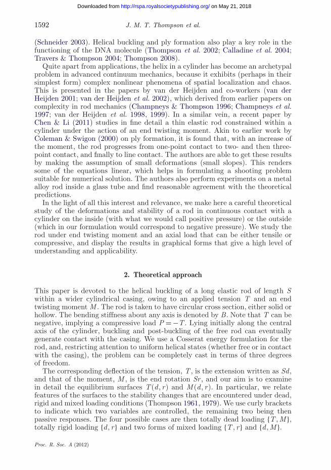
Figure 1. Some basic experiments under rigid {d, r} loading, performed with the help of CharlieMcRobie (Comberton Village College). Here all units are arbitrary.
Defining the dimensionless load parameter, m := M/√
BT , the free rod (undertension) exhibits a subcritical bifurcation of helical post-buckling states atmc = 2, from which the rod would jump dynamically under {T , M }—where itwould eventually stabilize depends crucially on the dynamics and the gap size.Meanwhile under rigid loading, {d, r}, the rod is known to follow a spatiallylocalizing path which also emanates from the bifurcation point and is energeticallyfavourable (Thompson & Champneys 1996). This path eventually reaches a fold,from which a free rod would jump into a self-contacting loop or ply. The gapbetween the rod and casing will govern whether this jump is observed or not.A simple {d, r} experiment under fixed r and varying d in which there is no jumpis illustrated in figure 1. The buckle amplitude grows steady under decreasing d,and a contacting helix gradually extends along the tube. This steady growth ofa buckling deflection can be attributed to slight misalignment of the rod in thejaws of the drill-chucks that grip the loaded ends.
In this paper, we analyse first the helical deformations of the free rod, bysetting to zero derivatives of the total potential energy with respect to the internaltorsion, ti, the helical angle, b, and the helical radius, r. When we turn to analysethe rod in contact with its casing the last condition is replaced by the constraintr = rw, where rw is the effective radius of the casing. Meanwhile, the sign of ther derivative informs us about the pressure between the rod and casing.
The situation is illustrated schematically in figure 2. This shows the variationof the total potential energy, V , of the free system at three values of m, two less
Proc. R. Soc. A (2012)
on May 21, 2018http://rspa.royalsocietypublishing.org/Downloaded from

1594 J. M. T. Thompson et al.
cylinder
contacting states
positive pressurezero pressurenegative pressure
stable
free states
unstablem
mc
V(r)
unstable post-buckling path
rmax
rw r
Figure 2. Schematic of the form taken by the free total potential energy at three values of m. Freeequilibrium solutions are illustrated by large balls, contacting solutions by the smaller balls.
than mc and one greater than mc. This energy is really a function of ti, b and r,but in this schematic diagram the variation with ti and b is ignored.
Concerning the range and scope of the study, we should note that T can bepositive or negative, a negative value corresponding to compression. Althoughwe mainly concentrate on positive T , the compression results are perfectly valid,though overall Euler buckling is impossible because of our assumed helical form.We also focus on positive M , with negative M simply giving mirror-image resultswith the helical angle reversed. We allow the helical angle, b, to range from−p to +p. When b is positive and equal to +p/2 the rod forms a ring, andmathematically (though not physically owing to the inevitable self-contacting ofthe rod) this ring can pass through itself to give a straight rod again at b = p.Negative b, generated by negative M , changes the handedness of the helix, anda mirror-image sequence can be generated as b decreases to −p. Finally, we cancontemplate either positive or negative pressure between the rod and its casing.Negative pressure could arise from magnetic or electrical attraction/repulsion, ormore simply if the rod were located outside a cylinder.
The paper is organized as follows. Section 3 has the main definitions forinternal and kinematic torsion, following the analysis of Love (1927). Some simplegeometrical formulae are defined for the total angle turned by the end moment,arc-wavelength, spatial frequency and end shortening. The large amplitudeequilibrium equations are derived from the total potential energy of the rod,
Proc. R. Soc. A (2012)
on May 21, 2018http://rspa.royalsocietypublishing.org/Downloaded from
Helical post-buckling 1595
rw
a
A
r
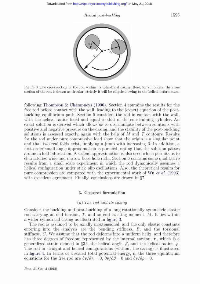
Figure 3. The cross section of the rod within its cylindrical casing. Here, for simplicity, the crosssection of the rod is drawn as circular; strictly it will be elliptical owing to the helical deformation.
following Thompson & Champneys (1996). Section 4 contains the results for thefree rod before contact with the wall, leading to the (exact) equation of the post-buckling equilibrium path. Section 5 considers the rod in contact with the wall,with the helical radius fixed and equal to that of the constraining cylinder. Anexact solution is derived which allows us to discriminate between solutions withpositive and negative pressure on the casing, and the stability of the post-bucklingsolutions is assessed exactly, again with the help of M and T contours. Resultsfor the rod under pure compressive load show that the origin is a singular pointand that two real folds exist, implying a jump with increasing b. In addition, afirst-order small angle approximation is pursued, noting that the solution passesaround a fold bifurcation. A second approximation is also used which permits us tocharacterize wide and narrow bore-hole radii. Section 6 contains some qualitativeresults from a small scale experiment in which the rod dynamically assumes ahelical configuration under stick–slip oscillations. Also, the theoretical results forpure compression are compared with the experimental work of Wu et al. (1993)with excellent agreement. Finally, conclusions are drawn in §7.
3. Cosserat formulation
(a) The rod and its casing
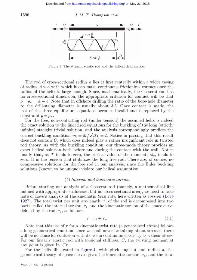
Consider the buckling and post-buckling of a long rotationally symmetric elasticrod carrying an end tension, T , and an end twisting moment, M . It lies withina wider cylindrical casing as illustrated in figure 3.
The rod is assumed to be axially inextensional, and the only elastic constantsentering into the analysis are the bending stiffness, B, and the torsionalstiffness, C . We assume that the rod deforms into a uniform helix, and thereforehas three degrees of freedom represented by the internal torsion, ti, which is ageneralized strain defined in §3b, the helical angle, b, and the helical radius, r.The rod in straight and helical configurations (without the casing) is illustratedin figure 4. In terms of a scaled total potential energy, v, the three equilibriumequations for the free rod are vv/vti = 0, vv/vb = 0 and vv/vr = 0.
Proc. R. Soc. A (2012)
on May 21, 2018http://rspa.royalsocietypublishing.org/Downloaded from
1596 J. M. T. Thompson et al.
r
S M TMT
L cos b
S cos b
b
D
Figure 4. The straight elastic rod and the helical deformation.
The rod of cross-sectional radius a lies at first centrally within a wider casingof radius A > a with which it can make continuous frictionless contact once theradius of the helix is large enough. Since, mathematically, the Cosserat rod hasno cross-sectional dimension, the appropriate criterion for contact will be thatr = rw = A − a. Note that in offshore drilling the ratio of the bore-hole diameterto the drill-string diameter is usually about 3.5. Once contact is made, thelast of the three equilibrium equations becomes invalid and is replaced by theconstraint r = rw.
For the free, non-contacting rod (under tension) the assumed helix is indeedthe exact solution to the linearized equations for the buckling of the long (strictlyinfinite) straight trivial solution, and the analysis correspondingly predicts thecorrect buckling condition mc = M/
√BT = 2. Notice in passing that this result
does not contain C , which does indeed play a rather insignificant role in twistedrod theory. As with the buckling condition, our three-mode theory provides anexact helical solution both before and during the contact with the wall. Noticefinally that, as T tends to zero, the critical value of the moment, Mc, tends tozero. It is the tension that stabilizes the long free rod. There are, of course, nocompressive solutions for the free rod in our analysis, since the Euler bucklingsolutions (known to be unique) violate our helical assumption.
(b) Internal and kinematic torsion
Before starting our analysis of a Cosserat rod (namely, a mathematical lineimbued with appropriate stiffnesses, but no cross-sectional area), we need to takenote of Love’s analysis of the kinematic twist rate, here written as torsion (Love1927). The total twist per unit arc-length, t, of the rod is decomposed into twoparts, called the internal torsion, ti, and the kinematic torsion of the space curvedefined by the rod, ts, as follows:
t = ti + ts. (3.1)
Note that this use of t for a kinematic twist rate (a generalized strain) followsa long geometrical tradition; since we shall never be talking about stresses, therewill be no cause for confusion with its use in continuum elasticity as a shear stress.For our linearly elastic rod with torsional stiffness, C , the twisting moment atany point is given by Ct.
For the helix illustrated in figure 4, with pitch angle b and radius r, thegeometrical theory of space curves gives the kinematic torsion, ts, and the total
Proc. R. Soc. A (2012)
on May 21, 2018http://rspa.royalsocietypublishing.org/Downloaded from
Helical post-buckling 1597
curvature, k, as
ts = sin b cos b
r(3.2)
and
k = sin2 b
r. (3.3)
The total angle in radians, R, turned by the end moment is given, using thetopological concepts of twist, link and writhe as in van der Heijden & Thompson(2000), by
r := RS
= ti + sin b
r= t + sin b(1 − cos b)
r, (3.4)
where S is the length of the (inextensional) rod. This expression is adequate forthe present investigation, being strictly correct for a long uniform helix that issupported in a manner similar to that envisaged by Love (1927). Notice that ris not given simply by t. If it were, we would find that under a prescribed endrotation, r , we would have a prescribed torsion, t, and a buckling deformationinto a helix would achieve no reduction in torsional strain energy (so there wouldbe no buckling).
We must finally write down some simple geometrical formulae that we shallneed in the following sections for the arc-wavelength, L, a non-dimensional spatialfrequency parameter, s, and the total axial end shortening of the deformed rod,D, as
L := 2pr
sin b, (3.5)
s := 2p
L
√BT
(3.6)
and d := DS
= 1 − cos b. (3.7)
Here, the word ‘arc’ emphasizes that we are defining these quantities in termsof arc-length along the curved rod, not along the straight central axis. Note thatthe dimension L cos b in figure 4 is commonly called the pitch of the helix.
(c) Energy formulation
We aim to derive, following Thompson & Champneys (1996), the largeamplitude equilibrium conditions for a rod deforming into a uniform helix whichcan make continuous frictionless contact with its outer casing. In particular, wewant to determine the equilibrium value of the helical angle b (and hence thewavelength L) in terms of the tension in the rod, T , and the twisting moment, M .
For this analysis (but not necessarily in its physical interpretation), we canregard T and M as prescribed dead (generalized) loads which do work throughthe corresponding deflections −D and R. Ignoring for the time being the contactwith the casing, the total potential energy, V , can then be treated as a functionof the three variables (ti, b, r).
Proc. R. Soc. A (2012)
on May 21, 2018http://rspa.royalsocietypublishing.org/Downloaded from
1598 J. M. T. Thompson et al.
The potential energies of T and M are VT and VM , respectively, given by
VT = TD = TS(1 − cos b) (3.8)
and
VM = −MR = −MS(
ti + sin b
r
). (3.9)
The strain energy of bending, VB, and the strain energy of torsion, VC, aregiven by
VB = 12BSk2 = 1
2BS sin4 b
r2(3.10)
and
VC = 12CSt2 = 1
2CS
(ti + sin b cos b
r
)2
. (3.11)
The total potential energy of the system, rod plus dead loads, is now
V := vS = VT + VM + VB + VC (3.12)
and the necessary and sufficient conditions for equilibrium of the freenon-contacting rod are that vv/vti = 0, vv/vb = 0 and vv/vr = 0.
The first equation gives us immediately
M = Ct. (3.13)
Whatever the (unspecified) boundary conditions are, equation (3.13) is anatural overall requirement, demanding that the end of the rod carries about itsown body axis the twisting moment M . The second equation gives, using (3.13),
Tr2 sin b + Mr(cos2 b − sin2 b − cos b) + 2B sin3 b cos b = 0 (3.14)
and the third equation gives, using (3.13),
vv
vr= [Mr(1 − cos b) − B sin3 b] sin b
r3= 0. (3.15)
Here, we have included the full expression for vv/vr, which we shall needsubsequently to characterize the contact pressure between the rod and the casing(where the derivative is not equal to zero). Equations (3.14) and (3.15) areinvariant under a simultaneous sign change of M and b, which is in line withthe handedness discussion of §2.
4. The free rod before contact
In this section, we look briefly at the response of the free rod. Note that ouranalysis will supply no non-trivial solutions under compression because it isrestricted to helical deformations. Although we prescribed dead T and M forour energy analysis, the equilibrium conditions that we have established do ofcourse hold for either rigid or dead loading. Having used (3.13) to eliminatet, the remaining equations (3.14) and (3.15) relate the loads (T , M ) to thegeneralized helical coordinates (b, r) for the free rod without wall contact. Note
Proc. R. Soc. A (2012)
on May 21, 2018http://rspa.royalsocietypublishing.org/Downloaded from
Helical post-buckling 1599
that these remaining full nonlinear equilibrium equations do not contain thetorsional stiffness C or the generalized coordinate ti. With a little manipulationthey can be written as
Tr2 = B sin2 b (4.1)
and
Mr = B sin3 b
1 − cos b, (4.2)
confirming that T ≥ 0.These two equations, (4.1) and (4.2), give T and M in terms of b and r, and
can be inverted to give b and r in terms of T and M .Defining the dimensionless load parameter,
m := M√BT
, (4.3)
we eliminate r between (4.1) and (4.2) to give the equation of the post-bucklingequilibrium path as m = sin2 b/(1 − cos b), which simplifies to
m = 1 + cos b (4.4)
and gives us the buckling load as mc = 2. Equation (4.4) is an exact answer for oneof the subcritical post-buckling paths of a long rod, because the assumed helixis indeed one of the buckling and post-buckling modes. For m > 2, when we arebeyond the subcritical buckling bifurcation, the only equilibrium solution is theunstable trivial state with b = 0. Note, however, that there is also a spatiallylocalized post-buckling path that is energetically favourable, and is alwaysobserved experimentally (Thompson & Champneys 1996). Substituting (4.4) backinto (4.1) to eliminate b, we get the equation for r as
g := r
√TB
= sin b =√
m(2 − m). (4.5)
Results of this exact free-rod analysis are plotted in figure 5. We notice thatr√
T/B reaches a maximum value of unity at m = 1. This will clearly influencewhether or not the rod makes contact with its casing.
Notice that using (3.5) and (4.1), we can immediately show that under all freeequilibrium conditions we have the universal result that
L = LU := 2p
√BT
or T = 4p2BL2
, (4.6)
showing that this arc-wavelength depends only on the load T , and that Ltends to infinity as T tends to zero. Had we chosen the axial wavelength, nosuch neat result would have been obtained. The second form of (4.6) makes aninstructive comparison with planar Euler buckling because the right-hand sideis the compressive critical load for a strut clamped at both ends. This can becompared, physically, with a single wave of the helix of axial length L cos b under
Proc. R. Soc. A (2012)
on May 21, 2018http://rspa.royalsocietypublishing.org/Downloaded from
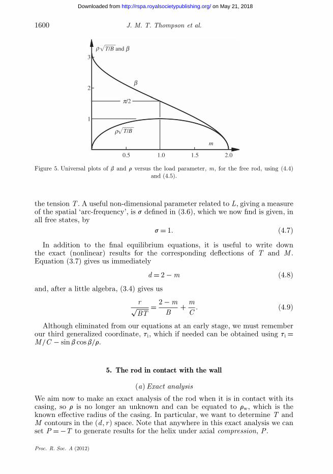
1600 J. M. T. Thompson et al.
b
p/2
r
r T/B and b
T/B
3
2
1
0.5 1.0 1.5
m
2.0
Figure 5. Universal plots of b and r versus the load parameter, m, for the free rod, using (4.4)and (4.5).
the tension T . A useful non-dimensional parameter related to L, giving a measureof the spatial ‘arc-frequency’, is s defined in (3.6), which we now find is given, inall free states, by
s = 1. (4.7)
In addition to the final equilibrium equations, it is useful to write downthe exact (nonlinear) results for the corresponding deflections of T and M .Equation (3.7) gives us immediately
d = 2 − m (4.8)
and, after a little algebra, (3.4) gives us
r√BT
= 2 − mB
+ mC
. (4.9)
Although eliminated from our equations at an early stage, we must rememberour third generalized coordinate, ti, which if needed can be obtained using ti =M/C − sin b cos b/r.
5. The rod in contact with the wall
(a) Exact analysis
We aim now to make an exact analysis of the rod when it is in contact with itscasing, so r is no longer an unknown and can be equated to rw, which is theknown effective radius of the casing. In particular, we want to determine T andM contours in the (d, r) space. Note that anywhere in this exact analysis we canset P = −T to generate results for the helix under axial compression, P.
Proc. R. Soc. A (2012)
on May 21, 2018http://rspa.royalsocietypublishing.org/Downloaded from
Helical post-buckling 1601
For the displacements, we have d from (3.7) and r from (3.4) and (3.13) as
d = 1 − cos b (5.1)
and
rrw = (1 + n)Mrw
B+ sin b(1 − cos b), (5.2)
where n is Poisson’s ratio introduced to represent the ratio of B to C via therelationship B/C = 1 + n, which is true for a solid circular elastic rod. Whennecessary, we take Poisson’s ratio as one-third (typical for a metal), givingB/C = 4/3.
It follows that for M contours we can immediately write down
rrw = rM (d)rw := (1 + n)Mrw
B± d
√d(2 − d), (5.3)
where the + sign corresponds to solutions with b > 0 and the − sign to solutionswith b < 0. For T contours, we first need to solve for M in terms of T and busing (3.14), after which we obtain
rrw = rT (d)rw := ±√
d(2 − d)[(1 + n)
2d(1 − d)(2 − d) + Tr2w/B
d(3 − 2d)+ d
]. (5.4)
Looking ahead to the ninth figure, we note that there is an asymptote atd = 3/2, separating small-d from large-d solutions. It means that at constantT no amount of applied moment M will make a solution path go pastb = arccos(−1/2) = 2p/3. There is a critical T contour (green) at the valueof Tr2
w/B = 3/4, for which the numerator and denominator in (5.4) aresimultaneously zero. This separates T contours that asymptote with r → +∞from those that asymptote with r → −∞, as we see in the ninth figure. We shouldremark here that solutions with b > p/2 are physically meaningful, but cannotbe reached in an experiment that starts from b = 0, since a real rod cannot passthrough (or indeed near to) the ring solution at b = p/2.
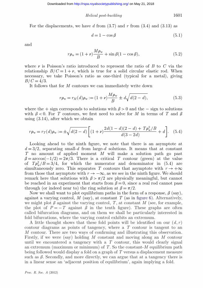
Now we shall want to plot equilibrium paths in the form of a response, b (say),against a varying control, M (say), at constant T (as in figure 6). Alternatively,we might plot b against the varying control, T , at constant M (see, for example,the plot of P = −T against b in the tenth figure). These graphs are oftencalled bifurcation diagrams, and on them we shall be particularly interested infold bifurcations, where the varying control exhibits an extremum.
A little thought shows that these fold points will be identified on our (d, r)contour diagrams as points of tangency, where a T contour is tangent to anM contour. There are two ways of confirming and illustrating this observation.Firstly, if we were (say) holding M constant and moving along an M contouruntil we encountered a tangency with a T contour, this would clearly signalan extremum (maximum or minimum) of T . So the constant-M equilibrium pathbeing followed would display a fold on a graph of T versus a displacement measuresuch as b. Secondly, and more directly, we can argue that at a tangency there isin a linear sense an ‘adjacent position of equilibrium’, again implying a fold.
Proc. R. Soc. A (2012)
on May 21, 2018http://rspa.royalsocietypublishing.org/Downloaded from
1602 J. M. T. Thompson et al.
–0.5 0.5 1.00–1.0–1.5–2.0 1.5 2.0 0.5
stable
stable
Mrw/BMrw/B
Trw2/B = 0.2
bb p = 0
p > 0
1.00
0.5
1.0
1.5
2.0
2.5
3.0
–2
–3
–1
0
1
2
3
(a) (b)
1.5 2.0
Figure 6. (a) Bifurcation diagrams for fixed T (Tr2w/B = −0.4 (dark green) to 1.2 (brown), in steps
of 0.2, from left to right at (say) b = 1) and (b) enlargement of the top right-hand quadrant withthe bifurcation diagram for Tr2
w/B = 0.2.
For a tangency of the M and T contours, and hence a fold in the M = const.or T = const. bifurcation diagram, we must have
rM (d) = rT (d) anddrM (d)
dd= drT (d)
dd. (5.5)
Using (5.3), (5.4) and (3.14) to eliminate m and T , this yields the tangencycurve given by
rrw = rt(d)rw := ±√
d(2 − d)[2(1 + n)
4 − 14d + 12d2 − 3d3
3 − 6d + 2d2+ d
]. (5.6)
A double fold (or cusp) occurs where this tangency curve is in turn tangent toboth the M and T contours (if it is tangent to the one it is also tangent to theother), i.e. where
rt(d) = rM (d) anddrt(d)
dd= drM (d)
dd. (5.7)
The second equation (5.7) reduces to a quintic in d with solution d = 0.172194,giving b = 0.595612 or 34.13◦ (independent of n). The first equation (5.7) thengives the critical value Mrw/B = 1.068666 and (5.4) gives the critical valueTr2
w/B = 0.349982. For loads larger than these critical values, there are no foldsand hence no stable solutions at small b. Both these critical values are universal,i.e. independent of n. The tangency curve has an asymptote at d = (3 − √
3)/2 �0.633975. It may also be verified that at d = 3/2 the tangency curve has rrw =(10 + n)
√3/12, which agrees with (5.4) after setting Tr2
w/B = 3/4, meaning thatthe tangency curve goes exactly through the critical saddle at d = 3/2. Theseresults can be seen later in the ninth figure (tangency curve in black).
We must next consider the pressure between the helical rod and the casing,and a measure of this pressure will be p := −(r3
w/B)vv/vr|r=rw, as illustratedschematically in figure 2. For simplicity, we will in future just call measure pthe pressure.
Proc. R. Soc. A (2012)
on May 21, 2018http://rspa.royalsocietypublishing.org/Downloaded from
Helical post-buckling 1603
By (3.15), a zero-pressure solution (which must obviously be a solution of thefree unconstrained rod) requires
Mrw
B= sin3 b
1 − cos b(5.8)
(there is also the trivial solution b = 0, for any M ). This gives the curve
rrw = ±√
d(2 − d)[2(1 + n) − nd]. (5.9)
Note that for non-zero solutions b ∈ (−p, p) a sign change of the pressurerequires M and b to have the same sign. For b > 0, the pressure is positive belowthe (+) curve, while for b < 0 it is positive above the (−) curve, where the signrefers to the sign in (5.9). The zero-pressure curve (orange in the ninth figure)intersects the tangency curve (black in the ninth figure) just before the latter’smaximum (for b > 0) or minimum (for b < 0), implying that there is always asign change of the pressure between the two (small-b) folds in either M = const.or T = const. bifurcation diagrams (confirmed in figure 6).
As we shall examine in the tenth figure, the T bifurcation diagram forpurely compressive buckling (M = 0) exhibits a jump instability at a fold.The corresponding critical load can be obtained from (3.14). Setting M = 0gives Tr2
w/B = −2 sin2 b cos b so that the condition for a fold, dT/db = 0, yieldsb = arccos(1/
√3) � 0.955317 (54.74◦). The critical compression is then found as
Tr2w/B = −4
√3/9 � 0.769800.
In the T bifurcation diagram, there is a special point at b = 2p/3 throughwhich all M contours pass. It corresponds to the branch d = 3/2 of the criticalcontour at Tr2
w/B = 3/4 in the ninth figure. All M contours intersect this branch.Finally, to determine the stability characteristics of the equilibrium paths
we compute the Hessian matrix, H , to check the second variation of the totalpotential energy
d2v = 12
v2v
vb2db2 + v2v
vbvtidbdti + 1
2v2v
vt2i
dt2i (5.10)
evaluated at a solution. Stability requires this matrix to be positive definite, whichis the case only if both the trace Tr(H ) and the determinant det(H ) are positive.We find that stability changes at folds, as expected, and the stability regimes areindicated in our final figures. Note that our notion of stability is restricted withinthe space of helical solutions.
To examine the results of the exact analysis, we look first in figure 6 atsome equilibrium paths in the bifurcation diagram. For a set of fixed T values,figure 6a shows the colour-coded equilibrium paths as the helical angle b againstthe twisting moment M . All equilibrium solutions in the b range of −p to +pare shown. The regimes in which the contact pressure is positive are shown ingrey. These regimes are bounded by the p = 0 curve in black. We remember thatwhere the pressure is zero we are at a post-buckling solution of the free rod, withinevitably m < 2. Figure 6b focuses on the red curves for Tr2
w/B = 0.2, and on
Proc. R. Soc. A (2012)
on May 21, 2018http://rspa.royalsocietypublishing.org/Downloaded from
1604 J. M. T. Thompson et al.
form of crossing(angles enlarged)
m = 2
m = 2
p = 0 crossing with d reversed(a)
index = 1 index = 0
minimumcircle colours for V:
positive negative unknown
valleysaddle
(b)
M
fold
fold
d, (b°)
rrw
2.0
1.5
1.0
0 0.1
stable(grey)
0.2 0.3(18) (32) (41)
T
(a) (b)
p < 0 m < 2
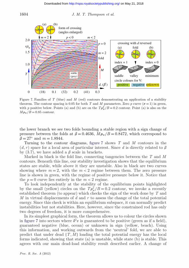
Figure 7. Families of T (blue) and M (red) contours demonstrating an application of a stabilitytheorem. The contour spacing is 0.05 for both T and M parameters. Zero p curve (s = 1) in green,with p positive below. Points (a) and (b) are on the Tr2
w/B = 0.2 contour. Point (a) is also on theMrw/B = 0.85 contour.
the lower branch we see two folds bounding a stable region with a sign change ofpressure between the folds at b = 0.4636, Mrw/B = 0.8472, which correspond tob = 27◦ and m = 1.8944.
Turning to the contour diagrams, figure 7 shows T and M contours in the(d, r) space for a local area of particular interest. Since d is directly related to bby (3.7), we have added a b scale in brackets.
Marked in black is the fold line, connecting tangencies between the T and Mcontours. Beneath this line, our stability investigation shows that the equilibriumstates are stable, while above it they are unstable. Also in black are two curvesshowing where m = 2, with the m < 2 regime between them. The zero pressureline is shown in green, with the regime of positive pressure below it. Notice thatthe p = 0 curve lies entirely in the m < 2 regime.
To look independently at the stability of the equilibrium points highlightedby the small (yellow) circles on the Tr2
w/B = 0.2 contour, we invoke a recentlyestablished theorem (to appear) which checks the sign of the work done by T andM in virtual displacements of d and r to assess the change of the total potentialenergy. Since this check is within an equilibrium subspace, it can normally predictinstabilities but not stabilities. Here, however, since the constrained rod has onlytwo degrees of freedom, it is more comprehensive.
In its simplest graphical form, the theorem allows us to colour the circles shownin figure 7 into sectors where d2v is guaranteed to be positive (green as if a field),guaranteed negative (blue, ocean) or unknown in sign (yellow, beach). Usingthis information, and working outwards from the ‘neutral’ fold, we are able topredict that under dead {T , M } loading the total potential energy has the localforms indicated, showing that state (a) is unstable, while state (b) is stable. Thisagrees with our main dead-load stability result described earlier. A change of
Proc. R. Soc. A (2012)
on May 21, 2018http://rspa.royalsocietypublishing.org/Downloaded from
Helical post-buckling 1605
br
d
0
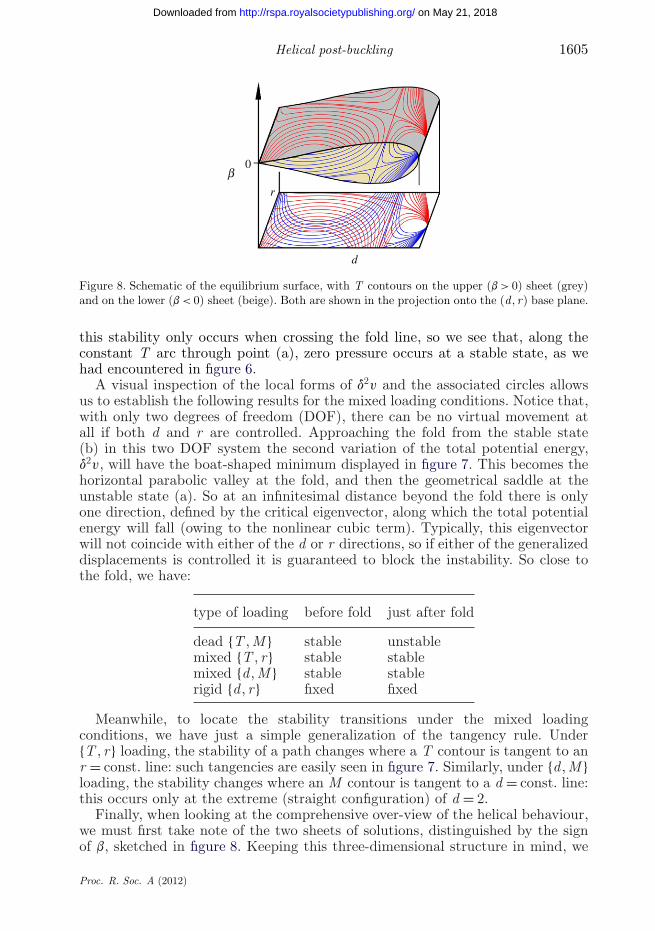
Figure 8. Schematic of the equilibrium surface, with T contours on the upper (b > 0) sheet (grey)and on the lower (b < 0) sheet (beige). Both are shown in the projection onto the (d, r) base plane.
this stability only occurs when crossing the fold line, so we see that, along theconstant T arc through point (a), zero pressure occurs at a stable state, as wehad encountered in figure 6.
A visual inspection of the local forms of d2v and the associated circles allowsus to establish the following results for the mixed loading conditions. Notice that,with only two degrees of freedom (DOF), there can be no virtual movement atall if both d and r are controlled. Approaching the fold from the stable state(b) in this two DOF system the second variation of the total potential energy,d2v, will have the boat-shaped minimum displayed in figure 7. This becomes thehorizontal parabolic valley at the fold, and then the geometrical saddle at theunstable state (a). So at an infinitesimal distance beyond the fold there is onlyone direction, defined by the critical eigenvector, along which the total potentialenergy will fall (owing to the nonlinear cubic term). Typically, this eigenvectorwill not coincide with either of the d or r directions, so if either of the generalizeddisplacements is controlled it is guaranteed to block the instability. So close tothe fold, we have:
type of loading before fold just after fold
dead {T , M } stable unstablemixed {T , r} stable stablemixed {d, M } stable stablerigid {d, r} fixed fixed
Meanwhile, to locate the stability transitions under the mixed loadingconditions, we have just a simple generalization of the tangency rule. Under{T , r} loading, the stability of a path changes where a T contour is tangent to anr = const. line: such tangencies are easily seen in figure 7. Similarly, under {d, M }loading, the stability changes where an M contour is tangent to a d = const. line:this occurs only at the extreme (straight configuration) of d = 2.
Finally, when looking at the comprehensive over-view of the helical behaviour,we must first take note of the two sheets of solutions, distinguished by the signof b, sketched in figure 8. Keeping this three-dimensional structure in mind, we
Proc. R. Soc. A (2012)
on May 21, 2018http://rspa.royalsocietypublishing.org/Downloaded from
1606 J. M. T. Thompson et al.
0.5 1.00
4(a)
(b)
2
0
–2
–4
4
2
0
–2
–41.5 2.0
rrw
rrw
d
stable
stableunstable
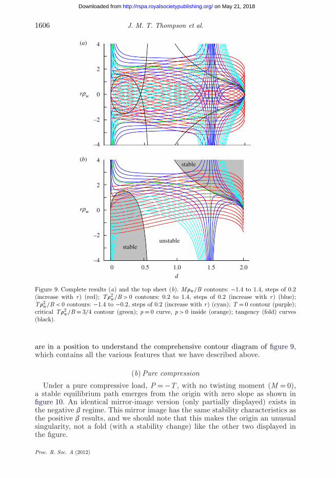
Figure 9. Complete results (a) and the top sheet (b). Mrw/B contours: −1.4 to 1.4, steps of 0.2(increase with r) (red); Tr2
w/B > 0 contours: 0.2 to 1.4, steps of 0.2 (increase with r) (blue);Tr2
w/B < 0 contours: −1.4 to −0.2, steps of 0.2 (increase with r) (cyan); T = 0 contour (purple);critical Tr2
w/B = 3/4 contour (green); p = 0 curve, p > 0 inside (orange); tangency (fold) curves(black).
are in a position to understand the comprehensive contour diagram of figure 9,which contains all the various features that we have described above.
(b) Pure compression
Under a pure compressive load, P = −T , with no twisting moment (M = 0),a stable equilibrium path emerges from the origin with zero slope as shown infigure 10. An identical mirror-image version (only partially displayed) exists inthe negative b regime. This mirror image has the same stability characteristics asthe positive b results, and we should note that this makes the origin an unusualsingularity, not a fold (with a stability change) like the other two displayed inthe figure.
Proc. R. Soc. A (2012)
on May 21, 2018http://rspa.royalsocietypublishing.org/Downloaded from
Helical post-buckling 1607
1.0
0.5
–0.5
–1.0–0.5 0 0.5 1.0
M = 0
jump
com
pres
sion
(–Tr w2
/B)
b1.5 2.0 2.5 3.0
0
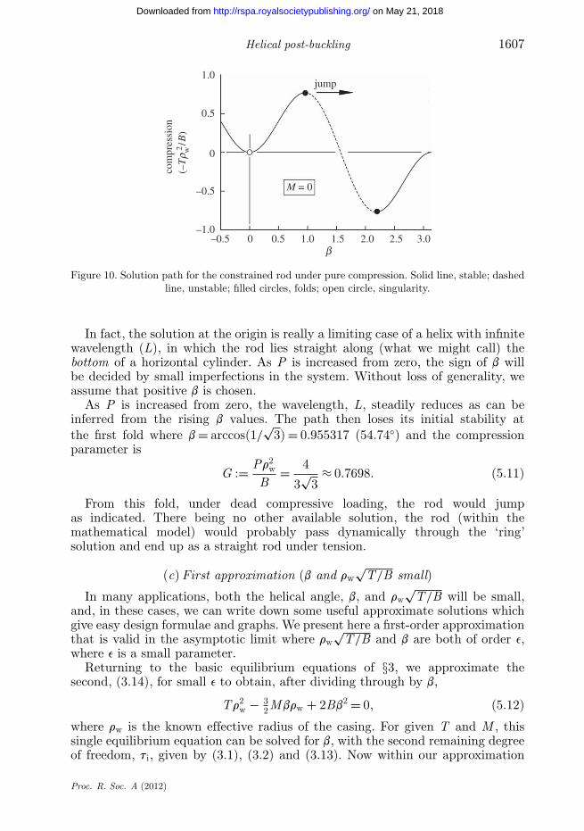
Figure 10. Solution path for the constrained rod under pure compression. Solid line, stable; dashedline, unstable; filled circles, folds; open circle, singularity.
In fact, the solution at the origin is really a limiting case of a helix with infinitewavelength (L), in which the rod lies straight along (what we might call) thebottom of a horizontal cylinder. As P is increased from zero, the sign of b willbe decided by small imperfections in the system. Without loss of generality, weassume that positive b is chosen.
As P is increased from zero, the wavelength, L, steadily reduces as can beinferred from the rising b values. The path then loses its initial stability atthe first fold where b = arccos(1/
√3) = 0.955317 (54.74◦) and the compression
parameter is
G := Pr2w
B= 4
3√
3≈ 0.7698. (5.11)
From this fold, under dead compressive loading, the rod would jumpas indicated. There being no other available solution, the rod (within themathematical model) would probably pass dynamically through the ‘ring’solution and end up as a straight rod under tension.
(c) First approximation (b and rw√
T/B small)
In many applications, both the helical angle, b, and rw√
T/B will be small,and, in these cases, we can write down some useful approximate solutions whichgive easy design formulae and graphs. We present here a first-order approximationthat is valid in the asymptotic limit where rw
√T/B and b are both of order e,
where e is a small parameter.Returning to the basic equilibrium equations of §3, we approximate the
second, (3.14), for small e to obtain, after dividing through by b,
Tr2w − 3
2Mbrw + 2Bb2 = 0, (5.12)
where rw is the known effective radius of the casing. For given T and M , thissingle equilibrium equation can be solved for b, with the second remaining degreeof freedom, ti, given by (3.1), (3.2) and (3.13). Now within our approximation
Proc. R. Soc. A (2012)
on May 21, 2018http://rspa.royalsocietypublishing.org/Downloaded from
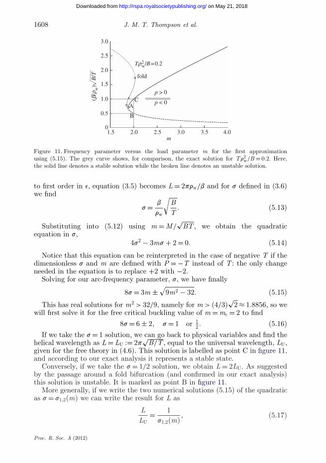
1608 J. M. T. Thompson et al.
B/T
(b/r
w)
3.0
2.5Tr2
w/B = 0.2
fold
CA
B
p > 0
p < 0
2.0
1.5
1.0
0.5
03.0 3.5 4.0
m2.52.01.5
Figure 11. Frequency parameter versus the load parameter m for the first approximationusing (5.15). The grey curve shows, for comparison, the exact solution for Tr2
w/B = 0.2. Here,the solid line denotes a stable solution while the broken line denotes an unstable solution.
to first order in e, equation (3.5) becomes L = 2prw/b and for s defined in (3.6)we find
s = b
rw
√BT
. (5.13)
Substituting into (5.12) using m = M/√
BT , we obtain the quadraticequation in s,
4s2 − 3ms + 2 = 0. (5.14)
Notice that this equation can be reinterpreted in the case of negative T if thedimensionless s and m are defined with P = −T instead of T : the only changeneeded in the equation is to replace +2 with −2.
Solving for our arc-frequency parameter, s, we have finally
8s = 3m ±√
9m2 − 32. (5.15)
This has real solutions for m2 > 32/9, namely for m > (4/3)√
2 ≈ 1.8856, so wewill first solve it for the free critical buckling value of m = mc = 2 to find
8s = 6 ± 2, s = 1 or 12 . (5.16)
If we take the s = 1 solution, we can go back to physical variables and find thehelical wavelength as L = LU := 2p
√B/T , equal to the universal wavelength, LU,
given for the free theory in (4.6). This solution is labelled as point C in figure 11,and according to our exact analysis it represents a stable state.
Conversely, if we take the s = 1/2 solution, we obtain L = 2LU. As suggestedby the passage around a fold bifurcation (and confirmed in our exact analysis)this solution is unstable. It is marked as point B in figure 11.
More generally, if we write the two numerical solutions (5.15) of the quadraticas s = s1,2(m) we can write the result for L as
LLU
= 1s1,2(m)
, (5.17)
Proc. R. Soc. A (2012)
on May 21, 2018http://rspa.royalsocietypublishing.org/Downloaded from
Helical post-buckling 1609
and the contacting solution for b as
b = rws1,2(m)
√TB
. (5.18)
Numerical results of this first approximation are shown in black in figure 11,where we observe a fold bifurcation at A that corresponds to the vanishing ofthe square root in equation (5.15) and is given by m = (4/3)
√2, s = 1/
√2 and
L/LU = √2. These results are compared with the exact solution for Tr2
w/B = 0.2in grey. As we would expect, there is good agreement at low b, up to the fold (atA in the approximation). After this, the two solutions diverge spectacularly,with the exact solution exhibiting a second fold that is not picked up at all in theblack curve.
The marked pressure change point (p = 0) merits some discussion. As we notedin the exact analysis, the zero pressure solution must be one of the free post-buckling equilibrium states. In these states, equation (4.7) gives us s = 1, andfigure 6 shows that non-trivial free states exist only for m < 2. Now the verticalaxis parameter of figure 11, namely (b/rw)
√B/T , is equal to s within the first
approximation, so, within this, we would conclude that the pressure is zero atC where m = 2. This is not possible, and points to a limitation of the firstapproximation. For the exact solution, the pressure change (marked by a greydiamond) is where the exact s is equal to unity, and this, plus the shift in thecurve, establishes that p = 0 is indeed at m < 2.
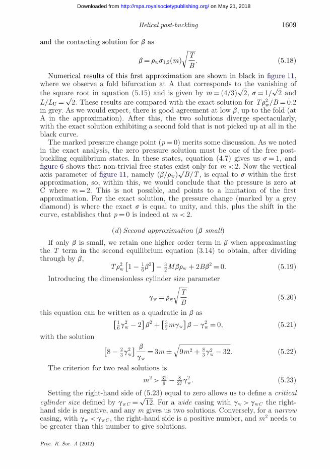
(d) Second approximation (b small)
If only b is small, we retain one higher order term in b when approximatingthe T term in the second equilibrium equation (3.14) to obtain, after dividingthrough by b,
Tr2w
[1 − 1
6b2] − 32Mbrw + 2Bb2 = 0. (5.19)
Introducing the dimensionless cylinder size parameter
gw = rw
√TB
(5.20)
this equation can be written as a quadratic in b as[ 16g2
w − 2]
b2 + [ 32mgw
]b − g2
w = 0, (5.21)
with the solution[8 − 2
3g2w
] b
gw= 3m ±
√9m2 + 8
3g2w − 32. (5.22)
The criterion for two real solutions is
m2 > 329 − 8
27g2w. (5.23)
Setting the right-hand side of (5.23) equal to zero allows us to define a criticalcylinder size defined by gwC = √
12. For a wide casing with gw > gwC the right-hand side is negative, and any m gives us two solutions. Conversely, for a narrowcasing, with gw < gwC , the right-hand side is a positive number, and m2 needs tobe greater than this number to give solutions.
Proc. R. Soc. A (2012)
on May 21, 2018http://rspa.royalsocietypublishing.org/Downloaded from
1610 J. M. T. Thompson et al.
3.0
2.5
2.0
1.5
1.0
0.5
03.0 3.5 4.0
m2.52.01.5
B/T
exact, Tr2w/B = 3
Tr2w/B = 3
(and exact)
gw = ½gwC
gw = 1/30
(b/r
w)
Figure 12. Solutions of the second approximation for two values of gw = rw√
T/B. The graph forgw = 1/30 is indistinguishable by eye from the first approximation and from the exact solutionshown in grey but is almost totally masked by the black. The extensive grey curve shows the exactsolution for Tr2
w/B = 3, which corresponds to half the critical gwC . Here, the solid line denotes astable solution while the broken line denotes an unstable solution.
We should remark here that when considering what is a ‘large’ rw we face theproblem that there is no other physical length dimension with which to compareits magnitude. We can make some progress by interpreting the dimensionlesscylinder size parameter, gw, defined in equation (5.20), as follows. Consider theradius of curvature, Rc, produced in the rod by a bending moment equal inmagnitude to T acting on a lever arm of length rw, which is given by Rc =B/(Trw). Substitution gives gw = √
rw/Rc, showing that gw is a measure of howlarge rw is compared with Rc. This helps a little, but depends on a knowledgeof the magnitude of T .
For two numerical studies, we give gw half its critical value, gw = (1/2)√
12, anda rather extreme figure of 1/30, as displayed in figure 12. These are compared withthe exact results, for the corresponding values of T (as given by equation (5.20)),and once again agreement is good for low b.
The two approximate solutions for the contacting rod give a great deal ofinsight, and useful universal graphs and parameters, for the practically relevantcase of small angles. The second approximation has the advantage of picking upthe existence of a critical cylinder diameter.
6. Remarks about drill-strings
(a) Historical drill-string studies
For many years, there has been a continuing thread of interest in the petroleumindustry on the helical buckling of drill-strings within their casing. Lubinskiet al. (1962) made calculations for the buckling of vertical tubing subjected tocompressive loading, without torsion, with and without packers (collars betweenthe tubing and casing). This was re-studied by Mitchell (1982), who includedthe boundary conditions at the ends where packers enforce alignment with the
Proc. R. Soc. A (2012)
on May 21, 2018http://rspa.royalsocietypublishing.org/Downloaded from
Helical post-buckling 1611
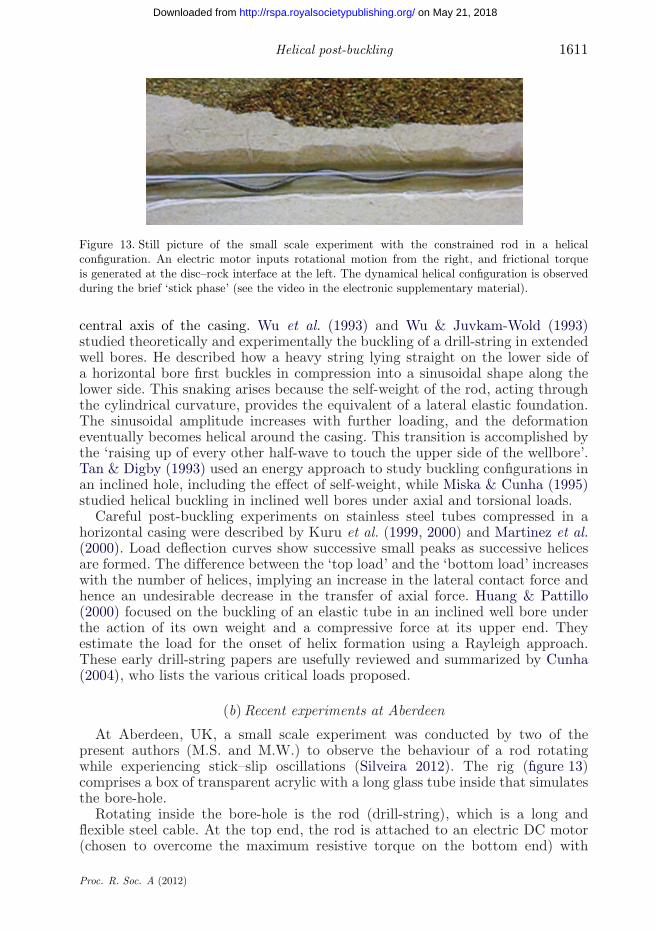
Figure 13. Still picture of the small scale experiment with the constrained rod in a helicalconfiguration. An electric motor inputs rotational motion from the right, and frictional torqueis generated at the disc–rock interface at the left. The dynamical helical configuration is observedduring the brief ‘stick phase’ (see the video in the electronic supplementary material).
central axis of the casing. Wu et al. (1993) and Wu & Juvkam-Wold (1993)studied theoretically and experimentally the buckling of a drill-string in extendedwell bores. He described how a heavy string lying straight on the lower side ofa horizontal bore first buckles in compression into a sinusoidal shape along thelower side. This snaking arises because the self-weight of the rod, acting throughthe cylindrical curvature, provides the equivalent of a lateral elastic foundation.The sinusoidal amplitude increases with further loading, and the deformationeventually becomes helical around the casing. This transition is accomplished bythe ‘raising up of every other half-wave to touch the upper side of the wellbore’.Tan & Digby (1993) used an energy approach to study buckling configurations inan inclined hole, including the effect of self-weight, while Miska & Cunha (1995)studied helical buckling in inclined well bores under axial and torsional loads.
Careful post-buckling experiments on stainless steel tubes compressed in ahorizontal casing were described by Kuru et al. (1999, 2000) and Martinez et al.(2000). Load deflection curves show successive small peaks as successive helicesare formed. The difference between the ‘top load’ and the ‘bottom load’ increaseswith the number of helices, implying an increase in the lateral contact force andhence an undesirable decrease in the transfer of axial force. Huang & Pattillo(2000) focused on the buckling of an elastic tube in an inclined well bore underthe action of its own weight and a compressive force at its upper end. Theyestimate the load for the onset of helix formation using a Rayleigh approach.These early drill-string papers are usefully reviewed and summarized by Cunha(2004), who lists the various critical loads proposed.
(b) Recent experiments at Aberdeen
At Aberdeen, UK, a small scale experiment was conducted by two of thepresent authors (M.S. and M.W.) to observe the behaviour of a rod rotatingwhile experiencing stick–slip oscillations (Silveira 2012). The rig (figure 13)comprises a box of transparent acrylic with a long glass tube inside that simulatesthe bore-hole.
Rotating inside the bore-hole is the rod (drill-string), which is a long andflexible steel cable. At the top end, the rod is attached to an electric DC motor(chosen to overcome the maximum resistive torque on the bottom end) with
Proc. R. Soc. A (2012)
on May 21, 2018http://rspa.royalsocietypublishing.org/Downloaded from
1612 J. M. T. Thompson et al.
Pr w2 /
B (
× 1
03 )
Prw2/B = 4d
d (× 103)
experiment
theoreticalslope
1 2
20
10
3
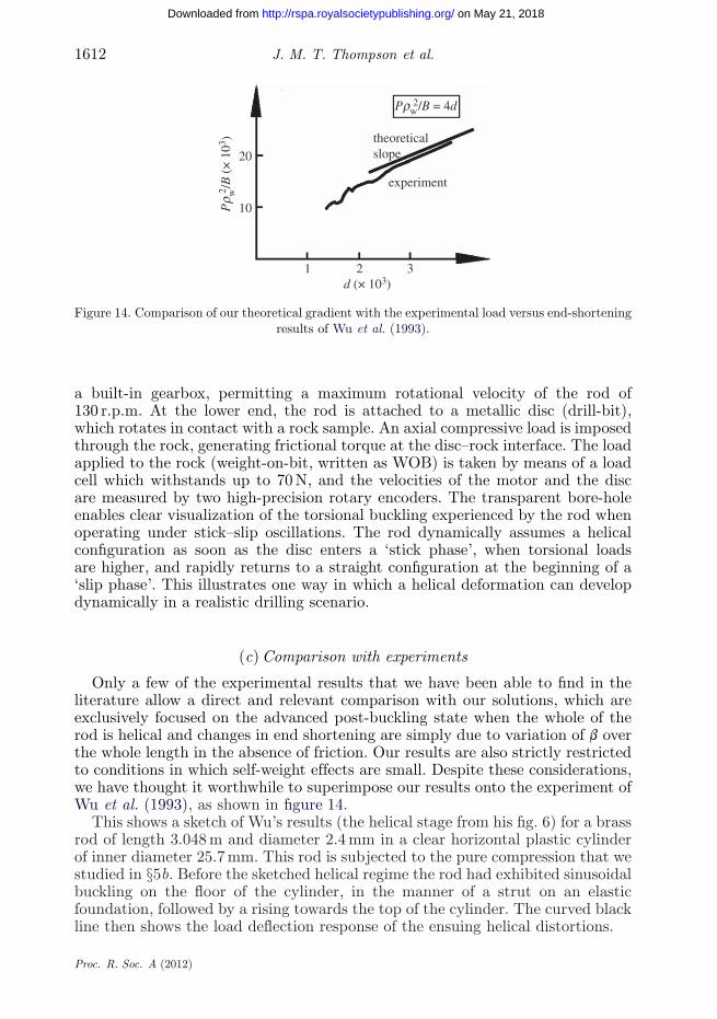
Figure 14. Comparison of our theoretical gradient with the experimental load versus end-shorteningresults of Wu et al. (1993).
a built-in gearbox, permitting a maximum rotational velocity of the rod of130 r.p.m. At the lower end, the rod is attached to a metallic disc (drill-bit),which rotates in contact with a rock sample. An axial compressive load is imposedthrough the rock, generating frictional torque at the disc–rock interface. The loadapplied to the rock (weight-on-bit, written as WOB) is taken by means of a loadcell which withstands up to 70 N, and the velocities of the motor and the discare measured by two high-precision rotary encoders. The transparent bore-holeenables clear visualization of the torsional buckling experienced by the rod whenoperating under stick–slip oscillations. The rod dynamically assumes a helicalconfiguration as soon as the disc enters a ‘stick phase’, when torsional loadsare higher, and rapidly returns to a straight configuration at the beginning of a‘slip phase’. This illustrates one way in which a helical deformation can developdynamically in a realistic drilling scenario.
(c) Comparison with experiments
Only a few of the experimental results that we have been able to find in theliterature allow a direct and relevant comparison with our solutions, which areexclusively focused on the advanced post-buckling state when the whole of therod is helical and changes in end shortening are simply due to variation of b overthe whole length in the absence of friction. Our results are also strictly restrictedto conditions in which self-weight effects are small. Despite these considerations,we have thought it worthwhile to superimpose our results onto the experiment ofWu et al. (1993), as shown in figure 14.
This shows a sketch of Wu’s results (the helical stage from his fig. 6) for a brassrod of length 3.048 m and diameter 2.4 mm in a clear horizontal plastic cylinderof inner diameter 25.7 mm. This rod is subjected to the pure compression that westudied in §5b. Before the sketched helical regime the rod had exhibited sinusoidalbuckling on the floor of the cylinder, in the manner of a strut on an elasticfoundation, followed by a rising towards the top of the cylinder. The curved blackline then shows the load deflection response of the ensuing helical distortions.
Proc. R. Soc. A (2012)
on May 21, 2018http://rspa.royalsocietypublishing.org/Downloaded from
Helical post-buckling 1613
The corresponding result from our exact theory is
Pr2w
B= 2d(1 − d)(2 − d) ≈ 4d, (6.1)
where the right-hand approximation is amply justified by the very lowexperimental d values. Now the nature of Wu’s experimental plot, including as itdoes the early non-helical deformations, precludes any sensible comparison withour equation as a whole. However, positioning this straight-line solution close toWu’s advanced helical deformations, we see that the gradients are in excellentagreement.
7. Concluding remarks
The buckling and post-buckling of an elastic rod deforming helically in contactwith a surrounding cylindrical casing of larger diameter has taken its place asan archetypal problem in modern continuum mechanics. In particular, complexnonlinear phenomena of spatial localization and chaos have been presented inthe papers van der Heijden (2001) and van der Heijden et al. (2002). In thispaper, we have presented new and extensive Cosserat solutions for the advancedpost-buckling stage under torsion and either tensile or compressive loading.Detailed stability and contact-pressure investigations have been made and theresults are presented with equilibrium surfaces to add insight and facilitatecomparisons with experimental results. One such experimental comparison, infigure 14, is extremely encouraging. Two approximate solutions give universalgraphs, parameters and design formulae, for the practically relevant case ofsmall angles, and highlight for the first time the existence of a critical cylinderdiameter. The results will be of interest to researchers in many areas of scienceand technology, including petroleum engineers and surgeons working with stents.
References
Calladine, C. R., Drew, H. R., Luisi, B. F. & Travers, A. A. 2004 Understanding DNA, 3rd edn.London, UK: Elsevier Academic Press.
Champneys, A. R. & Thompson, J. M. T. 1996 A multiplicity of localized buckling modes fortwisted rod equations. Proc. R. Soc. Lond. A 452, 2467–2491. (doi:10.1098/rspa.1996.0132)
Champneys, A. R., van der Heijden, G. H. M. & Thompson, J. M. T. 1997 Spatially complexlocalization after one-twist-per-wave equilibria in twisted circular rods with initial curvature.Phil. Trans. R. Soc. Lond. A 355, 2151–2174. (doi:10.1098/rsta.1997.0115)
Chen, J. & Li, H. 2011 On an elastic rod inside a slender tube under end twisting moment. J. Appl.Mech. 78, 041009-1. (doi:10.1115/1.4003708)
Coleman, B. D. & Swigon, D. 2000 Theory of supercoiled elastic rings with self-contact and itsapplication to DNA plasmids. J. Elast. 60, 173–221. (doi:10.1023/A:1010911113919)
Cunha, J. C. 2004 Buckling of tubulars inside wellbores: a review on recent theoretical andexperimental works. SPE Drill Completion 19, 13–19. (doi:10.2118/87895-PA)
Huang, N. C. & Pattillo, P. D. 2000 Helical buckling of a tube in an inclined wellbore. Int. J.Nonlinear Mech. 35, 911–923. (doi:10.1016/S0020-7462(99)00067-0)
Kuru, E., Martinez, A., Miska, S. & Qiu, W. 1999 The buckling behavior of pipes and its influenceon the axial force transfer in directional wells. In Proc. SPE/IADC Drilling Conf., Amsterdam,The Netherlands, 9–11 March 1999. SPE 52840. Society of Petroleum Engineers.
Proc. R. Soc. A (2012)
on May 21, 2018http://rspa.royalsocietypublishing.org/Downloaded from
1614 J. M. T. Thompson et al.
Kuru, E., Martinez, A., Miska, S. & Qiu, W. 2000 The buckling behavior of pipes and its influenceon the axial force transfer in directional wells. ASME J. Energy Resour. Tech. 122, 129–135.(doi:10.1115/1.1289767)
Love, A. E. H. 1927 A treatise on the mathematical theory of elasticity, 4th edn. Cambridge, UK:Cambridge University Press.
Lubinski, A., Althouse, W. S. & Logan, J. L. 1962 Helical buckling of tubing sealed in packers.Pet. Trans. 14, 655–670. (doi:10.2118/178-PA)
Martinez, A., Miska, S., Kuru, E. & Sorem, J. 2000 Experimental evaluation of the lateralcontact force in horizontal wells. ASME J. Energy Resour. Technol. 122, 123–128. (doi:10.1115/1.1289392)
Miska, S. & Cunha, J. C. 1995 An analysis of helical buckling of tubulars subjected to axial andtorsional loading in inclined wellbores. In Proc. SPE Production Operations Symp., OklahomaCity, OK, 2–4 April 1995. SPE 29460. Society of Petroleum Engineers.
Mitchell, R. F. 1982 Buckling behavior of well tubing: the packer effect. SPEJ 22, 616–624.(doi:10.2118/9264-PA)
Schneider, P. A. 2003 Endovascular skills: guidewire and catheter skills for endovascular surgery.New York, NY: Dekker.
Silveira, M. 2012 A comprehensive model of drill-string dynamics using Cosserat rod theory. PhDdissertation, School of Engineering, University of Aberdeen, UK.
Tan, X. C. & Digby, P. J. 1993 Buckling of drill string under the action of gravity and axial thrust.Int. J. Solids Struct. 30, 2675–2691. (doi:10.1016/0020-7683(93)90106-H)
Thompson, J. M. T. 1961 Stability of elastic structures and their loading devices. J. Mech. Eng.Sci. 3, 153–162. (doi:10.1243/JMES_JOUR_1961_003_021_02)
Thompson, J. M. T. 1979 Stability predictions through a succession of folds. Phil. Trans. R. Soc.Lond. A 292, 1–23. (doi:10.1098/rsta.1979.0043)
Thompson, J. M. T. 2008 Single-molecule magnetic tweezer tests on DNA: bounds on topoisomeraserelaxation. Proc. R. Soc. A 464, 2811–2829. (doi:10.1098/rspa.2008.0132)
Thompson, J. M. T. & Champneys, A. R. 1996 From helix to localized writhing in the torsionalpost-buckling of elastic rods. Proc. R. Soc. Lond. A 452, 117–138. (doi:10.1098/rspa.1996.0007)
Thompson, J. M. T., van der Heijden, G. H. M. & Neukirch, S. 2002 Supercoiling of DNAplasmids: mechanics of the generalized ply. Proc. R. Soc. Lond. A 458, 959–985. (doi:10.1098/rspa.2001.0901)
Travers, A. A. & Thompson, J. M. T. 2004 An introduction to the mechanics of DNA. Phil. Trans.R. Soc. Lond. A 362, 1265–1279. (doi:10.1098/rsta.2004.1392)
van der Heijden, G. H. M. 2001 The static deformation of a twisted elastic rod constrained to lieon a cylinder. Proc. R. Soc. Lond. A 457, 695–715. (doi:10.1098/rspa.2000.0688)
van der Heijden, G. H. M. & Thompson, J. M. T. 2000 Helical and localised buckling intwisted rods: a unified analysis of the symmetric case. Nonlinear Dyn. 21, 71–99. (doi:10.1023/A:1008310425967)
van der Heijden, G. H. M., Champneys, A. R. & Thompson, J. M. T. 1998 The spatial complexityof localized buckling in rods with non-circular cross-section. SIAM J. Appl. Math. 59, 198–221.(doi:10.1137/S0036139996306833)
van der Heijden, G. H. M., Champneys, A. R. & Thompson, J. M. T. 1999 Spatially complexlocalisation in twisted elastic rods constrained to lie in the plane. J. Mech. Phys. Solids 47,59–79. (doi:10.1016/S0022-5096(98)00095-7)
van der Heijden, G. H. M., Champneys, A. R. & Thompson, J. M. T. 2002 Spatially complexlocalisation in twisted elastic rods constrained to a cylinder. Int. J. Solids Struct. 39, 1863–1883.(doi:10.1016/S0020-7683(01)00234-7)
Wu, J. & Juvkam-Wold, H. C. 1993 Helical buckling of pipes in extended reach and horizontalwells. II. Frictional drag analysis. Trans. ASME 115, 196–201. (doi:10.1115/1.2905993)
Wu, J., Juvkam-Wold, H. C. & Lu, R. 1993 Helical buckling of pipes in extended reach andhorizontal wells. I. Preventing helical buckling. Trans. ASME 115, 190–195. (doi:10.1115/1.2905992)
Proc. R. Soc. A (2012)
on May 21, 2018http://rspa.royalsocietypublishing.org/Downloaded from