helicopter model syariful syafiq bin shamsudin universi
TRANSCRIPT

THE DEVELOPMENT OF AUTOPILOT SYSTEM FOR AN UNMANNED
AERIAL VEHICLE (UAV) HELICOPTER MODEL
SYARIFUL SYAFIQ BIN SHAMSUDIN
UNIVERSITI TEKNOLOGI MALAYSIA

iii
Dedication
This thesis is dedicated to:
My family for their patience and support during my study,
My friends for brightening my life with their friendship and showing me that life has
no greater reward to offer than a true friend.

iv
ACKNOWLEDGEMENTS
I believe that I am truly privileged to participate in this fascinating and
challenging project as a research member since 2004. I would like to give my deepest
gratitude to my supervisor Professor Ir. Dr. Hj. Abas Ab. Wahab, who has guided
and encouraged my work with such passion and sincerity for knowledge, teaching
and care. I would like also to thank Associate Professor Dr. Rosbi Mamat for his
guidance, insight and vision on this project.
I am pleased to acknowledge the financial support of Ministry of Higher
Education Malaysia (MOHE) via Research Management Centre (RMC), Universiti
Teknologi Malaysia under fundamental research grant vot 75124 and Tabung
Pembangunan Industri-UTM for scholarship awarded.
I would like to thank my research fellows Mohamad Hafiz Ismail, Nik
Ahmad Ridhwan and Mohd Syukri Ali for their help, advice and cooperation for
many years. I would like to thank Mohamed Yusof Radzak, Mohd Daniel Zakaria,
Mohd Anuar Adip and Nor Mohd Al Ariff Zakaria for encouraging and supporting
my research efforts in PIC programming, Control Theories, RC helicopter system
and hardware intergration.
I would like to thank all the technicians in Aeronautic and Robotic
Laboratories of Universiti Teknologi Malaysia for all the help given during the
development of test rig and autopilot system for UTM autonomous helicopter
project.
My speacial thanks go to my family. I would like to thank my parents, who
taught me to take chances for better things in my life. Also my gratitude to my
grandmother, who has offered me unconditional love and care. I thank my sisters for

v
their care and encouragement during my study and I would like to wish them all the
best in their studies and careers.
In retrospect, this project did start humble but has grown to be a success as
now. There are many happy times and many dispointing moments, but now I am
very happy because all the hardship I had to go through mostly alone finally paid off.
vi
ABSTRACT
The aim of this research project is to develop an autopilot system that enables
the helicopter model to carry out autonomous hover maneuver using on-board
intelligence computer. The main goal of this project is to provide a comprehensive
design methodology, implementation and testing of an autopilot system developed
for a rotorcraft-based unmanned aerial vehicles (UAV). The autopilot system was
designed to demonstrate autonomous maneuvers such as take-off and hovering flight
capabilities. For the controller design, the nonlinear dynamic model of the Remote
Control (RC) helicopter was built by employing Lumped Parameter approach
comprising of four different subsystems such as actuator dynamics, rotary wing
dynamics, force and moment generation process and rigid body dynamics. The
nonlinear helicopter mathematical model was then linearized using small
perturbation theory for stability analysis and linear feedback control system design.
The linear state feedback for the stabilization of the helicopter was derived using
Pole Placement method. The overall system consists of the helicopter with an on-
board computer and a second computer serving as a ground station. While flight
control is done on-board, mission planning and human user interaction take place on
ground. Sensors used for autonomous operation include acceleration, magnetic field,
and rotation sensors (Attitude and Heading Reference System) and ultrasonic
transducers. The hardware, software and system architecture used to autonomously
pilot the helicopter were described in detailed in this thesis. Series of test flights were
conducted to verify autopilot system performance. The proposed hovering controller
has shown capable of stabilizing the helicopter attitude angles. The work done for
this project gives solid bases and chances for fast evolution of Universiti Teknologi
Malaysia autonomous helicopter research.

vii
ABSTRAK
Hasrat utama projek penyelidikan ini adalah untuk membangunkan satu
sistem pemanduan automatik bagi membolehkan model helikopter menjalankan misi
berautonomi dengan hanya menggunakan keupayaan pengkomputeran pintar. Tesis
ini disediakan adalah untuk menerangkan dengan terperinci kaedah rekabentuk,
pelaksanaan dan pengujian sistem pemanduan automatik yang dibangunkan pada
pesawat rotor tanpa juruterbang. Sistem pemanduan automatik direka bagi
melakukan misi berautonomi seperti penerbangan berlepas dan apungan. Bagi
rekabentuk pengawal, model dinamik tidak linear bagi helikopter kawalan jauh telah
dibina menggunakan kaedah Pengumpulan Parameter melibatkan empat subsistem
yang berbeza yang terdiri daripada dinamik badan tegar, aktuator, sayap berputar dan
proses penghasilan daya dan momen. Model matematik helikopter tidak linear yang
diperolehi akan dilinearkan menggunakan teori perubahan kecil untuk kegunaan
analisis kestabilan dan rekabentuk suapbalik linear. Suapbalik keadaan linear untuk
penstabilan helikopter dapat diperolehi menggunakan kaedah Penetapan Kutub.
Sistem keseluruhan terdiri daripada sebuah komputer pada helikopter dan komputer
kedua sebagai pengkalan bumi. Pengawalan helikopter dijalankan oleh komputer
helikopter manakala operasi perancangan misi dan interaksi pengguna dilakukan di
pengkalan bumi. Penderia yang digunakan untuk operasi berautonomi termasuklah
penderia pecutan, medan magnet dan putaran serta penderia ultrasonik. Sistem
perkakasan dan perisian yang digunakan untuk pemanduan berautonomi helikopter
telah dibincangkan dengan lebih lanjut dalam tesis ini. Beberapa siri ujikaji
penerbangan telah dijalankan bertujuan untuk mengesahkan prestasi sistem
pemanduan automatik. Pengawal apungan yang direka didapati mampu untuk
menstabilkan sudut gayalaku penerbangan helikopter. Kerja-kerja yang dijalankan
untuk projek ini diharap dapat dijadikan asas dan peluang yang baik untuk
memangkin penyelidikan helikopter berautonomi Universiti Teknologi Malaysia.

viii
TABLE OF CONTENTS
CHAPTER TITLE PAGE TITLE i DECLARATION ii DEDICATION iii ACKNOWLEDGEMENT iv ABSTRACT vi ABSTRAK vii TABLE OF CONTENTS viii LIST OF TABLES xi LIST OF FIGURES xiii LIST OF SYMBOLS xix LIST OF APPENDICES xxiii
1 INTRODUCTION 1 1.1 Background of the Research 1 1.2 Research Problem Description 3 1.3 Research Objective 4 1.4 Research Scope 4 1.5 Research Design and Implementation 5 1.6 Project Contribution 7 1.7 Thesis Organization 7
2 LITERATURE REVIEW 9 2.1 Introduction 9 2.2 Principle of Rotary Wing Aircraft 11 2.2.1 The Different of Model Scaled and Full
Scaled Helicopter 18
2.3 Helicopter Dynamics Modeling and System Identification
21
2.4 Helicopter Control 24 2.4.1 Model Based Control 24 2.4.2 Model-Free Helicopter Control 27 2.5 Related Work 29 2.6 Summary 31
ix
3 HELICOPTER DYNAMIC MODELING 33 3.1 Introduction 33 3.2 Helicopter Parameters 36 3.2.1 Physical Measurement 36 3.2.2 Moment Inertia 38 3.2.3 Rotor Flapping Moment 40 3.2.4 Aerodynamic Input 40 3.2.5 Control Rigging Curve 42 3.3 Helicopter Model 45 3.4 Linearized Model 49 3.5 Main Rotor Forces and Moments 51 3.5.1 Quasi Steady State equations for Main
Rotor Dynamics 69
3.5.2 Control Rotor Model 72 3.6 Tail Rotor 78 3.7 Fuselage 79 3.8 Stabilizer Fins 81 3.9 Eigenvalues and Dynamic Mode 86 3.10 Conclusion 93
4 CONTROL SYSTEM ANALYSIS 95 4.1 Introduction 95 4.2 Regulation Layer 96 4.3 State Space Controller Design 98 4.3.1 Attitude Controller Design 99 4.3.2 Velocity Control 103 4.3.3 Heave and Yaw Control 104
4.3.4 Position Control 107
4.4 Conclusion 109
5 SYSTEM INTEGRATION 110 5.1 Introduction 110 5.2 Air Vehicle Descriptions 110 5.3 System Overview 118 5.4 Computers 119
5.4.1 PIC Microcontroller Programming Overview
121
5.5 Sensors 128 5.6 Communications 132 5.7 On-Board Computer Circuit 135 5.8 System Integration 138 5.8.1 Power Systems 139

x
5.8.2 Mounting 139 5.8.3 Component Placement 141 5.8.4 Electromagnetic and Radio Frequency
Interference (RFI) 144
5.8.5 Interfacing into the Radio Control System
144
5.9 Conclusion 147
6 SYSTEM EVALUATION 148 6.1 Introduction 148 6.2 Helicopter Support Structure 150 6.3 Preliminary Testing 151 6.3.1 AHRS Reading Test 152 6.3.2 Servo Routine Testing 155 6.3.3 Manual to Automatic Switch Testing 155 6.4 Flight Test 156 6.4.1 Manual Flight 156 6.4.2 Initial Flight Test 164 6.4.3 Partial Computer Controlled Flight 165 6.5 Conclusion 168
7 CONCLUSION 169 7.1 Concluding Remarks 169 7.2 Recommendation of Future Work 171 REFERANCES 172 APPENDIX A 182 APPENDIX B 185 APPENDIX C 189 APPENDIX D 205 APPENDIX E 211

xi
LIST OF TABLES
TABLE NO. TITLE
PAGE
2.1 Level of rotor mathematical modeling
23
3.1 Parameters of Raptor .90 helicopter for simulation model
37
3.2 Listing of variables used to determine the moments of inertia for the Raptor .90
39
3.3 Average value of moment of inertia used in simulation models
39
3.4 Analytically obtained F matrix in hover with no control rotor
86
3.5 Analytically obtained G matrix in hover with no control rotor
86
3.6 Eigenvalues and modes for six DOF model in hovering flight condition
87
3.7 Analytically obtained F matrix in hover with control rotor
89
3.8 Analytically obtained G matrix in hover with no control rotor
89
3.9 Eigenvalues and modes for eight DOF model in hovering flight condition.
90
4.1 Maximum values for height response parameters-hover and low speed according to ADS-33C
105
5.1 Helicopter PWM receiver output channels
115
5.2 The PIC18F2420/2520/4420/4520 family device overview
120
5.3 Rotomotion AHRS3050AA specifications 130

xii
5.4 EasyRadio ER400TRS transceiver pinout diagram
133
5.5 Weight and balance log
143
6.1 SANWA RD8000 transmitter setup 160
xiii
LIST OF FIGURES
FIGURE NO. TITLE
PAGE
1.1 The research project implementation flow chart
6
2.1 The total lift-thrust force acts perpendicular to the rotor disc or tip-path plane
13
2.2 Forces acting on helicopter in hover and vertical flight
13
2.3 Forces acting on the helicopter during forward, sideward and rearward flight
14
2.4 Tail rotor thrust compensates for the effect of the main rotor
15
2.5 Effect of blade flapping on lift distribution at advancing and retreating blade
17
2.6 Cyclic pitch variation in cyclic stick full forward position
17
2.7 Typical model scaled helicopter rotor head with hingeless Bell-Hiller stabilizer systems
19
2.8 The stabilizing effect of the Bell-Hiller stabilizer bar
21
2.9 SISO representations of helicopter dynamics
25
3.1 Raptor Aircraft’s 0.90 cu in (15 cc) aircraft manufactured by Thunder Tiger Corporation, Taiwan
34
3.2 X-Cell .60 rotor head designs showing the main blade attachment
35
3.3 The stabilizer bar mechanical system operation in RC helicopter
36
3.4 Raptor Precision Pitch Gauge manufactured by Thunder Tiger Corporation
42

xiv
3.5 The longitudinal cyclic rigging curve
43
3.6 The collective rigging curve
43
3.7 The lateral cyclic rigging curve
44
3.8 The directional control rigging curve
44
3.9 Typical arrangement of component forces and moments generation in helicopter simulation model
45
3.10 Free body diagram of scaled model helicopter in body coordinate system
48
3.11 Wind axes of helicopter in forward flight
49
3.12 Rotor flow states in axial motion. (a) Hover condition (b) Climb condition and (c) Descent condition
52
3.13 Induced velocity variation as a function of climb and descent velocities based on the simple momentum theory for Raptor .90
55
3.14 Inflow solutions for Raptor .90 from momentum theory
59
3.15 Rotor thrust or wing lift for Raptor .90 calculated from momentum theory
60
3.16 Azimuth angle reference point for clockwise rotor rotation viewed from above used mainly in most remote control helicopter manufactured outside US
62
3.17 Rotor swashplate and flapping angles relationship
62
3.18 Cross coupling due to the 3δ angle
64
3.19 Hub plane, tip path plane and body axes notations
67
3.20 Control rotor of the Raptor .90 helicopter
75
3.21 Force and moment generated from tail rotor sub-system
79
3.22 The horizontal and vertical stabilizer of Raptor .90
82
3.23 Poles of coupled longitudinal and lateral motion for six DOF model with no control rotor
88
3.24 Poles of coupled longitudinal and lateral motion for eight DOF model with control rotor
90
xv
3.25(a) Roll (top) and pitch (below) rate frequency responses
to lateral cyclic for Raptor .90 and X-Cell .60 in hover condition
92
3.25(b) Roll (top) and pitch (below) rate frequency responses to longitudinal cyclic for Raptor .90 and X-Cell .60 in hover condition
93
4.1 Hierarchical vehicle control system
96
4.2 A State Space representation of a plant
98
4.3 Plant with state feedback
99
4.4 Limits on pitch (roll) oscillations – hover and low speed according to Aeronautical Design Standard for military helicopter (ADS-33C)
100
4.5(a) Attitude compensator design for pitch axis response due to 0.007 rad longitudinal cyclic step command.
101
4.5(b) Attitude compensator design for roll axis response due to 0.0291 rad lateral cyclic step command
102
4.6 Compliance with small-amplitude pitch (roll) attitude changes in hover and low speed requirement specified in Section 3.3.2.1 of the Military Handling Qualities Specification ADS-33C
102
4.7(a) Velocity compensator design for longitudinal velocity mode due to longitudinal cyclic step command
103
4.7(b) Velocity compensator design for lateral velocity mode due to lateral cyclic step command
104
4.8 Procedure for obtaining equivalent time domain parameters for height response to collective controller according to Aeronautical Design Standard for military helicopter (ADS-33C)
105
4.9 Heave dynamics compensator design due to collective pitch step command
106
4.10 Yaw dynamics compensator design due to tail rotor collective pitch step command.
106
4.11 Compliance with small-amplitude heading changes in hover and low speed requirement specified in Section 3.3.5.1 of the Military Handling Qualities Specification
107
xvi
ADS-33C
4.12(a) Helicopter responses due to 6m longitudinal position step command
108
4.12(b) Helicopter responses due to 6m lateral position step command
108
5.1 Thunder Tiger Raptor .90 class helicopter equipped with two stroke nitromethane engine with 14.9 cc displacement
111
5.2 Side frame system and engine mounting in Raptor .90 main structure
112
5.3 Swashplate mechanism
113
5.4 SANWA RX-611 receiver and actuator (servo) connections
116
5.5 The gyro automatically corrects changes in the helicopter tail trim by crosswind
117
5.6 SANWA RD8000 PPM/FM/PCM1/PCM2 hand held transmitter
118
5.7 Overview of autopilot system developed
119
5.8 The pinout diagram of PIC18F4520 microcontroller
120
5.9 Screen shot of PICBasic Pro Compiler IDE
121
5.10 PicBasic Pro programming flowchart in roll attitude stabilization
123
5.11 Attitude stabilization operations in roll attitude stabilization
124
5.12 Code fragment used in the initiate stage
125
5.13 Code fragment used in the switching stage
126
5.14 Code fragment used in the execution stage
127
5.15 The low dynamic AHRS (AHRS3050AA) from Rotomotion, LLC
129
5.16 The Polaroid 6500 Ranging module from SensComp
131
5.17 The RF04 and CM02 modules used in the research project
132

xvii
5.18 Easy Radio transceiver block diagram
133
5.19 MAX232 application circuit
134
5.20 Typical system block diagram
134
5.21 The minimum circuit required by the PIC16F877A in order to operate
135
5.22 The flight computer circuit board
136
5.23 Schematic design of on-board computer drawn in EAGLE version 4.13 by CadSoft
137
5.24 Generated board from schematic circuit drawn in EAGLE version 4.13 by CadSoft
138
5.25 The avionic box integration with UAV helicopter platform
140
5.26 The avionic box design and the mounting points to helicopter frames
141
5.27 Component placements on the avionic box
142
5.28 AHRS mounting design
142
5.29 The autopilot system integration into radio control system
145
5.30 Manual to automatic switch connections
146
5.31 Automatic-manual switch locations on the SANWA RD8000 transmitter
146
6.1 Six degree of freedom (DOF) testbed
149
6.2 The helicopter testbed geometry
149
6.3 Helicopter support structure mounting point
150
6.4 The spherical plain bearing
150
6.5 Testbed two DOF joint
151
6.6 AHRS output data format
153
6.7 LED connections to PIC18F4520 Port B 154
xviii
6.8 AHRS reading testing on protoboard
154
6.9 Manual to automatic switch operation testing
155
6.10 Carburetor adjustment chart
158
6.11 Throttle servo installations
160
6.12 Blade pitch and collective travel setting
161
6.13 Blade tracking adjustment
162
6.14 Flybar/Stabilizer bar paddles setup
162
6.15 Tail rotor blade pitch setting
163
6.16 Tail centering adjustment setting
164
6.17 The Initial flight test
165
6.18 Partially computer control flight test
166
6.19 Experiment results of attitude (roll angle) regulation by autopilot system
166
6.20 Experiment results of attitude (pitch angle) regulation by autopilot system
167
6.21 Experiment results of attitude (yaw angle) regulation by autopilot system
167

xix
LIST OF SYMBOLS
aM Main rotor blade lift curve slope
ao Lift curve slope
0a Rotor blade coning angle
1sa Longitudinal flapping with respect to a plane perpendicular to
the shaft
1sb Lateral flapping
cM Main rotor chord
hM Main rotor hub height above CG
hT Tail rotor height above CG
lH Stabilizer location behind CG
lT Tail rotor hub location behind CG
m Mass flow rate
nes Gear ratio of engine shaft to main rotor
nT Gear ratio of tail rotor to main rotor
p, q, r Angular velocities about the x-, y- and z- axes
rpm Rotation per minute
u, v, w Translational velocities along the three orthogonal directions
of the fuselage fixed axes system
au , av , aw Fuselage center of pressure velocities along x, y and z axis
wu , wv , ww Airmass (gust) velocity along x, y and z axis
v Velocity at various stations in the stream tube
iv Inflow at the disc
Vav Vertical stabilizer local v-velocity
Faw Fuselage local w-velocity

xx
Haw Local horizontal stabilizer w-velocity
x State vector
cx Control actuation sub-system state vector
fx Fuselage sub-system state vector
px Engine sub-system state vector
rx Rotor sub-system state vector
1A Lateral cyclic pitch
dA Rotor disc area
eAR Effective aspect ratio
1B Longitudinal cyclic pitch
αLC Lift curve slope from airfoil data
HLC α Horizontal tail lift curve slope
VLC α Vertical fin lift curve slope
0DC Profile drag coefficient of the main rotor blade
FDC Fuselage drag coefficient
MDoC Main rotor blade zero lift drag coefficient
maxMTC Main rotor max thrust coefficient
TDoC Tail rotor blade zero lift drag coefficient
maxTTC Tail rotor max thrust coefficient
QC Torque coefficient
CG Center gravity
Ixx Rolling moment of inertia
Iyy Pitching moment of inertia
Izz Yawing moment of inertia
Iβ Main rotor blade flapping inertia
Kβ Hub torsional stiffness
l Distance from the pivot to the body CG
oI Moment contribution of the supporting structure
SMP + Oscillating period

xxi
PWM Pulse width modulation
eQ Engine torque
R, M, N Moment terms in roll, pitch and yaw directions
RM Main rotor radius
RT Tail rotor radius
HS Effective horizontal fin area
SV Effective vertical fin area FxS Frontal fuselage drag area
FyS Side fuselage drag area
FzS Vertical fuselage drag area
Sβ Stiffness number
T Rotor thrust
cV Climb velocity
dV Rotor descent velocity
W Weight of the UAV’s model
X, Y, Z Forces term in x, y, z directions FuuX , F
vvY , FwwX Fuselage effective flat plat drag in the x, y and z axis
VuuY Vertical stabilizer’s aerodynamic chamber effect
VuvY Vertical stabilizer’s parameter for lift slope effect
minHZ Horizontal stabilizer’s parameter for stall effect
HuuZ Horizontal stabilizer’s aerodynamic chamber effect
HuwZ Horizontal stabilizer’s parameters for lift slope effect
trimrδ Tail rotor pitch trim offset
0λ , 1cλ , 1sλ Rotor uniform and first harmonic inflow velocities in
hub/shaft axes
iλ Inflow ratio at rotor disc
βλ Flapping frequency ratio
colδ , lonδ , latδ , pedδ Main rotor collective pitch, longitudinal cyclic, lateral cyclic
and tail rotor collective
xxii
γ Lock number
γfb Stabilizer bar Lock number
ρ Atmosphere density
µ Advance ratio
θ , φ , Ψ Euler angles defining the orientation of the body axes relative
to the earth
0θ Local blade pitch
1θ Blade twist angle
ψ Rotor blade azimuth angle
Ω Main rotor speed
nomΩ Nominal main rotor speed
Subscript
M, T, F, H, V Representation for main rotor, tail rotor, fuselage, horizontal
stabilizer and vertical stabilizer

xxiii
LIST OF APPENDICES
Appendix TITLE
PAGE
A System and Control Matrices
182
B Pitch Mechanism Of Stabilizer And Main Rotor Blades
185
C Microcontroller Programming Code
189
D PIC18F2420/2520/4420/4520 Microcontroller Pinout Descriptions
205
E List of Publications
211
CHAPTER 1
INTRODUCTION
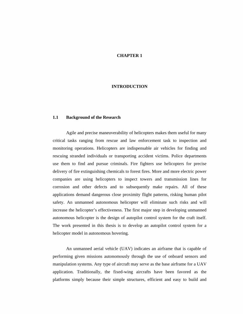
1.1 Background of the Research
Agile and precise maneuverability of helicopters makes them useful for many
critical tasks ranging from rescue and law enforcement task to inspection and
monitoring operations. Helicopters are indispensable air vehicles for finding and
rescuing stranded individuals or transporting accident victims. Police departments
use them to find and pursue criminals. Fire fighters use helicopters for precise
delivery of fire extinguishing chemicals to forest fires. More and more electric power
companies are using helicopters to inspect towers and transmission lines for
corrosion and other defects and to subsequently make repairs. All of these
applications demand dangerous close proximity flight patterns, risking human pilot
safety. An unmanned autonomous helicopter will eliminate such risks and will
increase the helicopter’s effectiveness. The first major step in developing unmanned
autonomous helicopter is the design of autopilot control system for the craft itself.
The work presented in this thesis is to develop an autopilot control system for a
helicopter model in autonomous hovering.
An unmanned aerial vehicle (UAV) indicates an airframe that is capable of
performing given missions autonomously through the use of onboard sensors and
manipulation systems. Any type of aircraft may serve as the base airframe for a UAV
application. Traditionally, the fixed-wing aircrafts have been favored as the
platforms simply because their simple structures, efficient and easy to build and

2
maintain. The autopilot design is easier for fixed-wing aircrafts than for rotary-wing
aircrafts because the fixed-wing aircrafts have relatively simple, symmetric, and
decoupled dynamics.
However, rotorcraft-based UAVs have been desirable for certain applications
where the unique flight capability of the rotorcraft is required. The rotorcraft can take
off and land within limited space and they can also hover, and cruise at very low
speed. The agile maneuverability of model scaled helicopter or remote control (RC)
helicopter sold in commercial market can be useful for an unmanned surveillance
helicopter in a hard to reach or inaccessible environment such as city and mountain
valley. Unmanned surveillance helicopter offers a lot benefits in search and rescue
operations, remote inspections, aerial mapping and offer an alternative option for
saving human pilot from dangerous flight conditions (Amidi, 1996).
Beside these advantages, helicopters are well known to be unstable and have a
faster and responsive dynamics due to their small size. Model scaled helicopter can
reach pitch and roll rates up to 200 deg/s with stabilizer bar, yaw rates up to 1000
deg/s and produces thrust as high as two or three times the vehicle weight (Mettler et
al., 2002a). The helicopter dynamics are inherently unstable and require velocity
feedback as well as attitude feedback to stabilize and control. Velocity feedback
needs the accurate velocity estimates, which can be obtained by the use of an inertial
navigation system. The inertial navigation system in turn requires external aids so
that the velocity and position estimates do not diverge with the uncompensated bias
and drift of the inertial instruments, i.e., accelerometers and rate gyroscopes. Another
irony is that, even though UAVs are typically smaller than the full-size manned
vehicles, they usually require more accurate sensors because the demanded sensor
accuracy is higher when the vehicle is smaller.
An autopilot system is a mechanical, electrical, or hydraulic system used to
guide a vehicle without assistance from a human being. In the early days of transport
aircraft, aircraft required the continuous attention of a pilot in order to fly in a safe
manner and results to a very high fatigue. The autopilot is designed to perform some
of the tasks of the pilot. The first successful aircraft autopilot was developed by
Sperry brothers in 1914 where the autopilot developed was capable of maintaining

3
pitch, roll and heading angles. Lawrence Sperry has demonstrated the effectiveness
of the design by flying his aircraft with his hands up (Nelson, 1998). Modern
autopilots use computer software to control the aircraft. The software reads the
aircraft's current position and controls a flight control system to guide the aircraft.
As an unmanned vehicle, issues such as remote sensing, terrain and obstacle
recognition, radio link and data acquisition must be solved for absolute reliability.
The design must be proven to work given the constraints of the environment especially
due to lack of immediate and flexible human intervention available on board. An
autonomous control mechanism should be able to accommodate and manage all of
the issues mentioned above in real-time. It also must be able to plan its flight and
mission goals without continuous human guidance. As general remarks, the
autonomous helicopter is built basically by putting together state-of-the-art
navigation sensors and high performance onboard computer system with real-time
software control on commercially available remote-control helicopter model (Shim,
2000). The autonomous unmanned helicopter system design problem alone
encompasses many challenging research topics such as system identification, control
system architecture and design, navigation sensor design and implementation, hybrid
systems, signal processing, real-time control software design, and component-level
mechanical-electronic integration. The vehicle communicates with other agents and
the ground posts through the broadband wireless communication device, which will
be capable of dynamic network internet protocol (IP) forwarding. The vehicle will be
truly autonomous when it is capable of self-start and automatic recovery with a
single click of a button on the screen of the vehicle-monitoring computer.
1.2 Research Problem Description
Among many issues that must be addressed in the important area of
autonomous helicopter, this thesis will cover three important issues only, i.e. the
helicopter mathematical modeling and identification, hardware, software and system
integration and control system design. To begin with, in order to determine the most
effective control strategy that governs the overall architecture of a model scaled

4
helicopter, a detailed knowledge of the structure and functions of the helicopter in
the form of a mathematical model is necessary. Secondly, the analytical
mathematical model must then be provided with physical parameters accurately
representing a real helicopter model. This analytical mathematical model of
helicopter is important for the design of an autopilot system that provides
artificial stability to improve flying qualities of helicopter model. Lastly, a good
waypoint navigation planning method that fundamentally guides an on-board
computer control mechanism must be devised.
1.3 Research Objective
The objective of this research study is to develop an autopilot system that
could enable the helicopter model to perform autonomous hover maneuver using
only on-board intelligence and computing power.
1.4 Research Scope
The scopes set forth for the research work as follows:
i. Establishing scaled helicopter model dynamic characteristics for the
control system design of autopilot system
ii. Developing an electronic control system that enables the helicopter
model to perform its mission goal.
iii. Fabricating and testing the electronic control system (autopilot)
performance on helicopter model in autonomous hovering.

5
1.5 Research Design and Implementation
In order to design an autopilot system for scaled model helicopter, a
performance and stability analysis will be conducted using several physical
measurements, experimental testing and similarity analysis. The helicopter model is
derived from a general full-sized helicopter with the augmentation of servo rotor
dynamics. The nonlinear model derived from general full-sized helicopter model will
be simplified through linearization in order to obtain a linear model controller design.
The helicopter platform was then integrated with navigation sensors and onboard
flight computer. Linearized control theory will be applied for helicopter stabilization
using the model obtained. After the design of low-level vehicle stabilization
controller, vehicle guidance logic will be developed. The vehicle guidance logic can
be used as a user interface part on the ground station and sequencer on the UAV side.
The complete autopilot system integration with the helicopter had been done after all
the electronics were built and installed considering several factors such as power
requirement, mounting, electromagnetic and radio interference. The implementation
of the project research is shown in Figure 1.1

6
Figure 1.1 The research project implementation flow chart
Start
Literature Review
System Identification and Modeling of Helicopter Dynamic
Hardware and Vehicle Integration
The Design of Control System • Attitude Control • Speed Control • Heave and Yaw Control
Flight Test to Determine Helicopter Performance under Autonomous Control of the Autopilot System
Finish
Report Writing
7
1.6 Project Contribution
The project contributions are as follows:
i. Simulation models for controller design, stability and performance
analysis of a UAV helicopter model had been developed.
ii. The low level stabilization controller had been designed based on the
control theory developed from the simulation model.
iii. The prototype of autopilot system integration with the helicopter was
developed taking into consideration the power requirement, mounting,
electromagnetic and radio interference.
iv. A prototype of UAV helicopter capable of hovering autonomously
had been developed. This is the major break through in the effort of
developing a completely autonomous UAV helicopter.
1.7 Thesis Organization
This thesis is organized into seven chapters. The first chapter introduced the
motivation, research objective, scopes of work and contribution of this project.
Chapter 2 reviews the UAV development history, principle of rotary wing
aircraft, helicopter dynamic modeling, control and autonomous system design are
also explained in this chapter.
Chapter 3 presents the helicopter dynamic modeling procedures and
simulation results while Chapter 4, Hardware, Software and Vehicle Integration,
described the hardware and software development of the system and system
integration into the helicopter model.
Chapter 5 presents the control design methodology and result for each
controller for the autopilot system.

8
Chapter 6 presents the flight test conducted in order to test the functionality
of the autopilot system. The preliminary tests were also conducted to ensure that the
system developed works properly.
In the final chapter, Chapter 7, the research work is summarized and the
potential future works are outlined.

CHAPTER 2
LITERATURE REVIEW
2.1 Introduction
An unmanned aerial vehicle (UAV) can be defined as an airplane designed
with no pilot on board which can take over various roles of piloted aircraft. There are
a number of important fields of science and technology which are directly related to
UAV research such as aerodynamics, propulsion, structural, flight dynamic and
control, flight performance and electronic system integration into UAV platform.
An autonomous UAV indicates an airframe that is capable of performing
given missions autonomously through the use of onboard sensors and manipulation
systems. There are different types of aircraft which can be use as the base airframe
for a UAV application such as fixed wing aircraft and rotorcraft based UAV. Each
UAV capability varies significantly to each other and can also be categorized based
on their payload weight carrying capability, mission profile (altitude, range, duration)
and their command, control and data acquisition capabilities.
The fixed-wing aircraft have been favored as the platform for UAV because
of many good reasons: they are simple in structure, efficient, and easy to build and
maintain. The autopilot design is easier for fixed-wing aircrafts than for rotary-wing
aircrafts because the fixed-wing aircrafts have relatively simple, symmetric, and
decoupled dynamics (Shim, 2000). Some fixed wing UAVs such as Pioneer UAV

10
used by Marine Corps for example, have very successful records in actual field
operations (Office of The Secretary of Defense, 2005).
The rotorcraft-based UAVs have been desirable for certain applications
where the unique flight capability of the rotorcraft is required. The rotorcraft can
take-off and land within limited space and they can also hover, and cruise at very low
speed. Research of rotorcraft-based UAVs has finally become an active area during
the last decade although one of the first rotorcraft UAVs, Gyrodyne QH-50, made its
debut in 1958. The advance in rotorcraft UAV research could be achieved thanks to
the maturing technologies that became available during the last 10 years, such as
rotorcraft dynamics, control system theory and application, high-accuracy small
navigation systems and Global Positioning System (GPS) (Shim, 2000).
Building a custom-designed helicopter requires tremendous knowledge, time,
and effort. The market for the helicopter platform for rotorcraft UAV development is
very small and specialized. Most of the above reasons contribute to the general
understanding that rotorcraft UAVs are more expensive and more difficult to operate
than fixed wing UAVs. However, only rotorcraft UAVs can perform some
applications such as low-speed tracking maneuvers in law-enforcement,
reconnaissance, and operations where no runway is available for take-off and landing
(Amidi et al., 1998). Thanks to the vertical take-off and landing (VTOL) capability,
rotorcrafts can take off and land on a very limited space such as a ship deck (Naval
Air Systems Command, 2001). Hover, low speed flight and sideslip capabilities
make the helicopter a perfect vehicle for tracking or searching out ground targets. In
summary, the characteristics of rotorcraft UAVs are listed as follows:
Advantages:
i. Small space is required for launch and retrieval.
ii. Versatile flight modes: vertical take-off, landing, hover, pirouette, sideslip,
low-speed cruise.
Disadvantages:
i. More complicated mechanical structure.
ii. Inefficient flight dynamics: lower maximum speed, shorter mission range.

11
iii. More accurate and complicated navigation sensor requirement.
iv. Inherently unstable and relatively poorly known dynamics. Difficult control
system design.
2.2 Principle of Rotary Wing Aircraft
The helicopter is capable of several versatile flight modes mentioned in the
section earlier and able to cruise like a conventional aircraft. The fixed wing aircraft
obtained lift with their wings as they propel through the air with sufficient speed
while helicopter uses rotor to generate lift as it rotates horizontally above the
fuselage. The blade of the helicopter main rotor has a flexible high aspect ratio wing
and the pitch of each blade (or is called blade angle) can be altered to cause a change
in the blade’s angle of attack, thereby controlling the corresponding aerodynamic
forces (Montgomery, 1964). This in turn will control the total thrust generated by the
main rotor. The main rotor can be tilted as a disc to control its directional and
longitudinal motions by cyclic pitch control. The cyclic pitch angle is also called disc
angle.
In any kind of flight modes (hovering, vertical, forward, sideward, or
rearward), the total lift and thrust forces of a rotor are perpendicular to the tip-path
plane or plane of rotation of the rotor as shown in Figure 2.1. The tip-path plane is
the imaginary circular plane outlined by the rotor blade tips in making a cycle of
rotation. During any kind of horizontal or vertical flight, there are four forces acting
on the helicopter i.e. the lift, thrust, weight, and drag. Lift is the force required to
support the weight of the helicopter. Thrust is the force required to overcome the
drag on the fuselage and other helicopter components.
During hovering flight in a no-wind condition, the tip-path plane is horizontal
and parallel to the ground. Lift and thrust forces act straight up while weight and
drag act straight down. The sum of the lift and thrust forces must equal the sum of
the weight and drag forces in order for the helicopter to hover.

12
During vertical flight in a no wind condition, the lift and thrust forces both act
vertically upward while weight and drag both act vertically downward. As shown in
Figure 2.2, when lift and thrust equal weight and drag, the helicopter hovers. If lift
and thrust are less than weight and drag, the helicopter descends vertically and if lift
and thrust force are greater than weight and drag, the helicopter rises vertically.
During forward flight, the tip-path plane is tilted forward, thus tilting the total
lift-thrust force forward from the vertical. This resultant lift-thrust force can be
resolved into two components i.e. the lift acting vertically upward and thrust acting
horizontally in the direction of flight. In addition to lift and thrust, there are weights,
drag, the rearward acting or retarding force of inertia and wind resistance. In straight-
and-level unaccelerated forward flight, lift equals weight and thrust equals drag
(straight-and-level flight is flight with a constant heading and at a constant altitude).
If the lift exceeds the weight, the helicopter climbs; if the lift is less than the weight,
the helicopter descends. If the thrust exceeds the drag, the helicopter speeds up; if the
thrust is less than the drag, it slows down.
During sideward flight, the tip-path plane is tilted sideward in the direction
that flight is desired thus tilting the total lift-thrust vector sideward. In this case, the
vertical or lift component is still straight up, weight straight down but the horizontal
or thrust component now acts sideward with drag acting to the opposite side. The tip-
path plane is tilted rearward thus tilting the lift-thrust vector rearward in rearward
flight. The thrust components are rearward and drag forward, just the opposite to
forward flight. The lift component is straight up and weight straight down. The
forces acting on helicopter during forward, sideward and rearward flight are shown
in Figure 2.3.

13
Figure 2.1 The total lift-thrust force acts perpendicular to the rotor disc or tip-path plane (Federal Aviation Administration, 1973)
Figure 2.2 Forces acting on helicopter in hover and vertical flight (Federal Aviation Administration, 1973)

14
Figure 2.3 Forces acting on the helicopter during forward, sideward and rearward flight (Federal Aviation Administration, 1973)
As the main rotor of a helicopter turns in one direction, the fuselage tends to
rotate in the opposite direction. This tendency for the fuselage to rotate is called
torque. Torque effect on the fuselage is a direct result of engine power supplied to
the main rotor and any change in engine power brings about a corresponding change
15
in torque effect. The greater the engine power, the greater the torque effect will be. In
autorotation maneuver, there is no engine power being supplied to the main rotor and
thus there is no torque reaction created during autorotation.
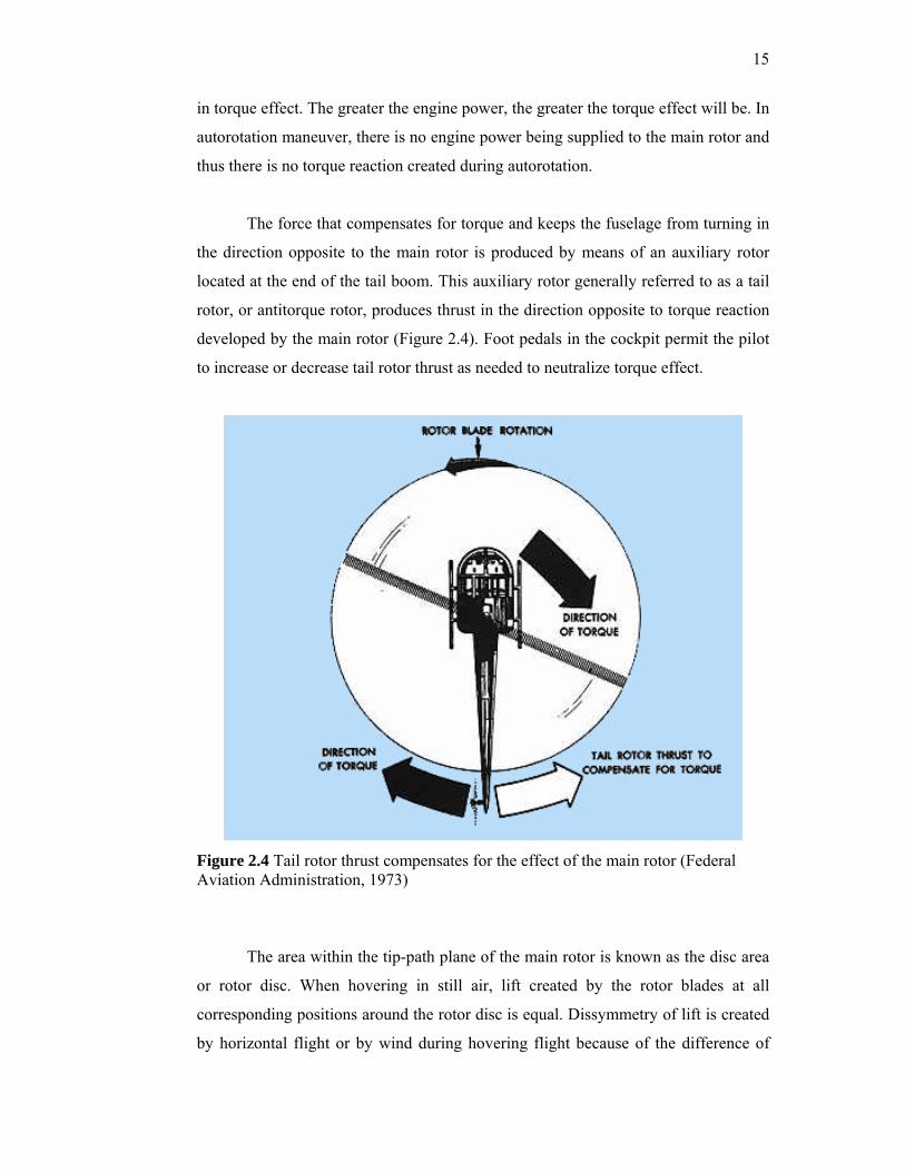
The force that compensates for torque and keeps the fuselage from turning in
the direction opposite to the main rotor is produced by means of an auxiliary rotor
located at the end of the tail boom. This auxiliary rotor generally referred to as a tail
rotor, or antitorque rotor, produces thrust in the direction opposite to torque reaction
developed by the main rotor (Figure 2.4). Foot pedals in the cockpit permit the pilot
to increase or decrease tail rotor thrust as needed to neutralize torque effect.
Figure 2.4 Tail rotor thrust compensates for the effect of the main rotor (Federal Aviation Administration, 1973)
The area within the tip-path plane of the main rotor is known as the disc area
or rotor disc. When hovering in still air, lift created by the rotor blades at all
corresponding positions around the rotor disc is equal. Dissymmetry of lift is created
by horizontal flight or by wind during hovering flight because of the difference of

16
velocities acting on advancing and retreating blades. Considering a case in which
each blade had the same pitch setting, lift is found to be larger at the advancing than
the retreating sides. This is due to the differences in velocity experienced by the
blades on the two different sides (Prouty, 1986). This would produce an unbalanced
rolling moment which could roll the helicopter over as can be shown in Figure
2.5(a).
Another important characteristic of the main rotor, in addition to thrust and
anti-torque is the flapping. Blade flapping compensates the dissymmetry of lift.
Blade flapping is the up and down movements of a rotor blade which in conjunction
with cyclic feathering causes dissymmetry of lift to be eliminated as shown in Figure
2.5(b). In a two-bladed system, the blades flap as a unit. As the advancing blade flaps
up due to the increased lift, the retreating blade flaps down due to the decreased lift.
The change in angle of attack on each blade brought about by this flapping action
tends to equalize the lift over the two halves of the rotor disc.
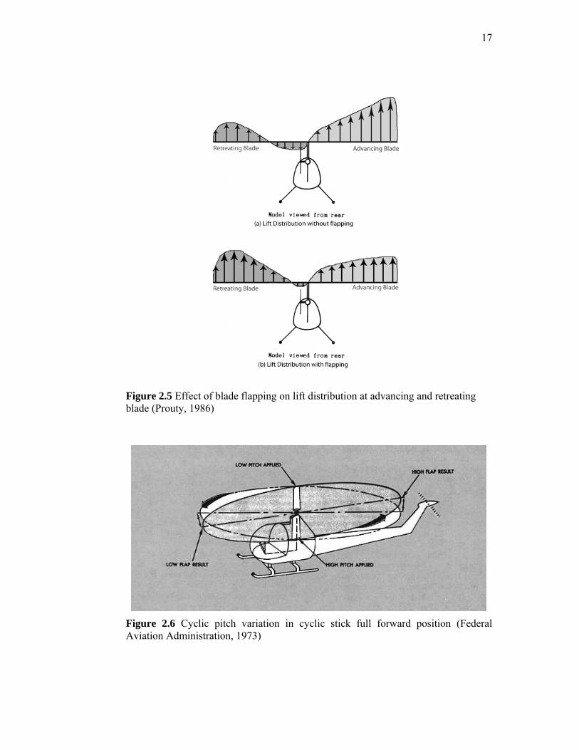
The position of the cyclic pitch control in forward flight also causes a
decrease in angle of attack on the advancing blade and an increase in angle of attack
on the retreating blade. Cyclic pitch which was created by tilting the swashplate
causes the mechanism to force the helicopter blade to have a certain pitch angle in
the function of azimuth (rotation angle of the main rotor referring to fuselage).
The spinning main rotor of the helicopter acts like a gyroscope in which the
blade pitch angle follows 90° in advance of swashplate angle in order to compensate
for the 90° phase delay of gyroscopic effect (Shim, 2000). Referring to Figure 2.6, as
each blade passes the 90° position on the left, the maximum increase in angle of
attack occurs. As each blade passes the 90° position to the right, the maximum
decrease in angle of attack occurs. Maximum deflection takes place 90° later where
maximum upward deflection occurs at the rear and maximum downward deflection
at the front. This resulting in tip-path plane tilts forward. Combining together the
effects from cyclic pitch control and blade flapping equalizes the lift over the two
halves of the rotor disc.
17
Figure 2.5 Effect of blade flapping on lift distribution at advancing and retreating blade (Prouty, 1986)
Figure 2.6 Cyclic pitch variation in cyclic stick full forward position (Federal Aviation Administration, 1973)

18
2.2.1 The Different of Model Scaled and Full Scaled Helicopter
A model helicopter is a miniaturization of a full-scale helicopter version but
there are significant differences between the two. The first major difference between
model and full-scale helicopters are the way the main rotor blades is attached to the
rotor head (Kim and Tilbury, 2000). Many full scale helicopters have a hinge, either
free-flapping or spring-mounted, on the rotor blades, so that the plane of the rotor
can be tilted with respect to the helicopter. Such a hinge system allows the rotor
blades to flap which increase helicopter stability. However, this flapping behavior
increases the time needed for the helicopter to respond to control inputs. By tilting
the rotor disc forward, the helicopter can move forwards while the fuselage remains
in level plane (Johnson, 1980).
Most helicopter models have a hingeless, stiff rotor hub design which forces
the position of the fuselage to remain fixed with respect to the rotor disc (Kim and
Tilbury, 2000). This results in faster response times, and gives the remote pilot a
better sense of motion of the helicopter. In most helicopter models, the rotors are
attached through a single lag hinge, as shown in Figure 2.7; there is no flap hinge
that would allow the blade to move out of the plane of rotation. The model
helicopters were design with no flap hinges because they are designed to operate at
relatively low translational velocities near hover condition (Bortoff, 1999). Thus, the
compensating the asymmetry of lift experienced with full-size helicopters at high
speed is not a design priority. In addition, many pilots perform stunt flying with their
helicopters. The rigidly attached disk makes certain maneuvers, such as inverted
flight, much easier than with an articulated rotor.

19
Figure 2.7 Typical model scaled helicopter rotor head with hingeless Bell-Hiller stabilizer systems
Secondly, scaled model radio control (RC) helicopter usually has a very high
rotor speed around 1500 rpm and fast dynamic response due to its small inertia value.
Shim (2000) had reported that in order for scaled model helicopter to achieve
equilibrium of lift on the rotor disc in less than one rotor revolution, most of the
small size helicopters would require response time in less than 40 milliseconds.
Without any extra stability augmentation devices, this is an extremely short time for
the radio control pilots on the ground to control the helicopters and for this reason,
almost all small-size radio helicopters have a mechanism to artificially introduce
damping. In most model helicopters, a large control gyro with an airfoil, referred to
as a stabilizer bar (flybar) is used to improve the stability characteristic around the
pitch and roll axes and to minimize the actuator force required. In addition, an
electronic gyro is used on the tail rotor to further stabilize the yaw axis. In most full
scale helicopters, the large rotor and fuselage inertias and the flapping rotor hinge
provide adequate stability, and extra control gyros on the rotors are unnecessary.
20
Model scaled helicopters are often equipped with mechanical stabilizer bar
design which the original concept came from full-scale helicopter stabilization
devices first used in the 1950s. The Bell stabilizing system had a bar with weights at
each end, and the flapping motion of the bar was governed by a separate damper. The
Hiller system replaced the damper and the weights with an airfoil. During the early
1970s, the design was simplified and applied for model-scale helicopters (Kim and
Tilbury, 2000). This system is often called a Bell-Hiller mixer, because it
incorporates some of design aspects of both Bell and Hiller designs. The rotor hub
design presented in Figure 2.7, hingeless with Bell-Hiller mixer, represents currently
the most popular and widely accepted design as the best compromise between
performance and stability. However, it is suited more towards aerobatic maneuvers
than smooth near-hover maneuvers that do not require large and fast pitch or roll
movements. Stability can be increased if the Bell input is removed and/or the main
blade is allowed to flap, but the helicopter would then respond more slowly (Kim and
Tilbury, 2000).
According to Mettler et al. (2002b), this system can be regarded as a
secondary rotor attached to the shaft either at the below or above the main rotor
position by an unrestrained teetering hinge. The stabilizer bar consists of two simple
paddles being attached to an essentially rigid rod. The stabilizer bar receives the
same cyclic pitch and roll inputs from the swash plate but no collective input. The
Bell-Hiller stabilizer bar used in model scaled helicopter as a blade angle actuator.
When a cyclic input is applied by the pilot, the stabilizer bar creates lift which tilts
the flybar disc. By applying the cyclic control to the flybar and allowing the flybar to
apply a secondary cyclic input to the main blade, the servo load is significantly
reduced compared to condition where the cyclic input were applied directly to main
blades.
The motion of Bell-Hiller stabilizer bar is connected to the main rotor pitch
levers through series of linkages. According to Shim (2000), Bell-Hiller stabilizer bar
behaves as a gyroscope maintaining the current attitude of rolling and pitching for
substantial time. Considering the helicopter model in Figure 2.8, in a hovering
condition, the stabilizer bar angle β is known to be zero (level). If a wind gust or
other disturbance knocks the helicopter out of its equilibrium, the stabilizer bar
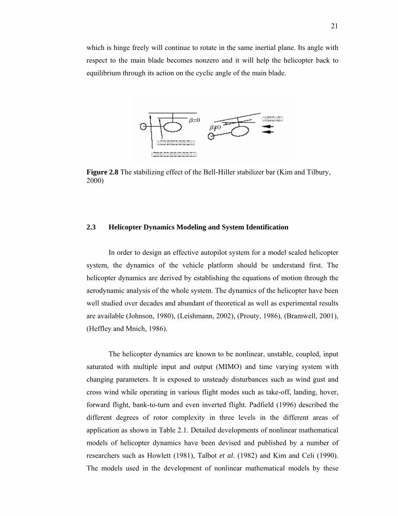
21
which is hinge freely will continue to rotate in the same inertial plane. Its angle with
respect to the main blade becomes nonzero and it will help the helicopter back to
equilibrium through its action on the cyclic angle of the main blade.
Figure 2.8 The stabilizing effect of the Bell-Hiller stabilizer bar (Kim and Tilbury, 2000)
2.3 Helicopter Dynamics Modeling and System Identification
In order to design an effective autopilot system for a model scaled helicopter
system, the dynamics of the vehicle platform should be understand first. The
helicopter dynamics are derived by establishing the equations of motion through the
aerodynamic analysis of the whole system. The dynamics of the helicopter have been
well studied over decades and abundant of theoretical as well as experimental results
are available (Johnson, 1980), (Leishmann, 2002), (Prouty, 1986), (Bramwell, 2001),
(Heffley and Mnich, 1986).
The helicopter dynamics are known to be nonlinear, unstable, coupled, input
saturated with multiple input and output (MIMO) and time varying system with
changing parameters. It is exposed to unsteady disturbances such as wind gust and
cross wind while operating in various flight modes such as take-off, landing, hover,
forward flight, bank-to-turn and even inverted flight. Padfield (1996) described the
different degrees of rotor complexity in three levels in the different areas of
application as shown in Table 2.1. Detailed developments of nonlinear mathematical
models of helicopter dynamics have been devised and published by a number of
researchers such as Howlett (1981), Talbot et al. (1982) and Kim and Celi (1990).
The models used in the development of nonlinear mathematical models by these

22
researchers were obtained using full scaled helicopter simulators. The models used
were of high orders with high numbers of degree of freedom and contained a large
number of parameters that often cannot be measured directly. The theoretical model
derived using aerodynamic equations in nonlinear mathematical model often gives a
large error due to the inaccurate knowledge of the actual parameters of aerodynamic
components and has to be validated and refined with the actual experimental results
(Shim, 2000).
For the reason mentioned above and for the purpose of this thesis, it has been
decided to adopt the parametric linear time-invariant model proposed by Mettler et
al. (1999) in order to identify the model scaled dynamic parameters. Mettler et al.
(2000a) performed a comprehensive study of the characteristics of small-scaled
helicopter dynamics. He developed and identified parameterized linear models for
hover and cruise flight conditions for the Yamaha R-50, using frequency domain
methods (CIFER) proposed by Tishler and Cauffman (1992). He later applied the
same parameterized model to MIT’s X-Cell .60, validating and extending the
observation that the rotor forces and moments largely dominate the dynamic
response of small-scaled helicopters. This significantly simplifies the modeling task.
Both the flight conditions were accurately modeled by a rigid-body model
augmented with the first-order rotor and stabilizer bar dynamics; no inflow dynamics
were necessary. The coupled rotor and stabilizer bar equations can be lumped into
one first-order effective rotor equation of motion (for both the lateral and
longitudinal tip-path-plane flapping). The linear models accurately captured the
vehicle dynamics for a relatively large region around the nominal operating point.
The model accurately predicted the vehicle angular response for aggressive control
inputs for the full range of angular motion. Subsequently, comparing results obtained
for the larger Yamaha R-50 (150lb, 5ft rotor radius), and smaller MIT’s X-Cell .60
(17lb, 2.5ft rotor radius), he showed that the former was dynamically similar to a
full-scale helicopter; its characteristics related to those of a full-scale vehicle through
Froude scaling rules. The latter, on the other hand, belonged to an entirely different
dynamic class; it related to the larger vehicle via Mach scaling rules, which predicted
a dramatic increase in agility with reduction of the vehicle size.

23
Table 2.1 Level of rotor mathematical modeling (Padfield, 1996)
Level 1 Level 2 Level 3
Aerodynamics
Linear 2-D Dynamic inflow/local Momentum theory Analytically integrated loads
Nonlinear (limited 3-D) Dynamic inflow/local Momentum theory Local effects of blade Vortex interaction Unsteady 2-D Compressibility Numerically integrated loads
Nonlinear 3-D Full wake analysis (free or prescribed) Unsteady 2-D Compressibility Numerically integrated loads
Dynamics
Rigid blades 1. quasi-steady motion 2. 3 DOF flap 3. 6 DOF flap + lag 4. 6 DOF flap + lag + quasi steady
torsion
1. rigid blades with options as in Level 1
2. limited number of blade elastic modes
Detailed structural representation as elastic modes or finite elements
Applications
Parametric trends for flying qualities and performance studies Well within operational flight envelope Low bandwidth control
Parametric trends for flying qualities and performance studies Medium bandwidth appropriate to high gain active flight control
Rotor design Rotor limit loads prediction Vibration analysis Rotor stability analysis Up to safe flight envelope

24
2.4 Helicopter Control
There have been a number of approaches for automated full-sized helicopter
control, both mathematically model-based i.e. (Amidi, 1996) and (Maharaj, 1994) as
well as other less traditional model-free controls i.e. (Phillips et al., 1996),
(Cavalcante et al., 1995). Kim (1993) has merged the two approaches.
In addition, the Association for Unmanned Vehicle Systems has sponsored a
yearly autonomous aerial robotics competition since 1991 (Michelson, 1994). Many
universities have been experimenting with RC model helicopters for entry into this
competition. These include, but are not limited to, Massachusetts Institute of
Technology, Boston University and Draper Laboratory (Debitetto et al., 1996),
University of Southern California (Montgomery et al., 1995), Georgia Institute of
Technology (Kahn and Kannan, 1995), Technische Universitat Berlin (Musial et al.,
1999), Southern Polytechnic State University (Burleson et al., 2001), Rose-Hulman
Institute of Technical (Groven et al., 2002), Simon Fraser University (Haintz et al.,
2003), University of Arizona (Dooley et al., 2003), University of Texas (Holifield et
al., 2003), Waterloo University (Behjat et al., 1999) and Stanford University
(Woodley et al., 1995).
2.4.1 Model Based Control
Some of the earliest modern research on helicopter control are the application
of Linear Quadratic Gaussian (LQR) theory on helicopter control and the hover
control with sling-load from the 1960s (Shim, 2000). After these works, there has
been much research done in the area of helicopter control utilizing various
approaches which can be categorized into:
i. Classical control theory (Hess, 1994), (Amidi, 1996)
ii. Linear quadratic regulation (Ingle and Celi, 1992), (Takahashi, 1994)
iii. Eigenstructure assignment (Mannes and Smith, 1992)

25
iv. Robust control theory such as H∞ (Ingle and Celi, 1992), (Walker and
Postlethwaite, 1991), (Reynolds and Rodriguez, 1992) or µ-synthesis
(Shim, 2000).
v. Rotor dynamics inclusion (Takahashi, 1994), (Ingle and Celi, 1992).
vi. Input-output linearization (Koo and Sastry, 1998).
These results allow insights on how the control system should be synthesized
for small-size helicopter dynamics. Since the classical control theory is only
applicable to SISO system, the MIMO helicopter dynamics should be decoupled into
SISO sub-system (Figure 2.9). The classical control theory is currently the most
favored method by military and industrial research communities due to the simple
and intuitive control system structure and more importantly it has been shown to be
effective in numerous flight tests.
Figure 2.9 SISO representations of helicopter dynamics (Shim, 2000)
One of the earliest works done in autonomous helicopter was by Amidi
(1996). Amidi had developed an autonomous helicopter system using vision as the
primary source of guidance and control. He applied linear control design techniques

26
to synthesize a proportional-derivative (PD) controller. In this approach, a simple,
literalized model of the helicopter around the hover condition was used. The
controller demonstrated hovering and low-speed (20 mph) point-to-point
maneuvering capability on a Yamaha R50 helicopter. The major advantage of this
approach is that minor on-line computations are required and there exist many
controller synthesis techniques for controller design. Montgomery and Bekey (1998)
had reported that two primary limitations exist with this approach. First, the
linearized model is an approximation and does not contain the more complete
information contained in a nonlinear model. Second, the linearized helicopter model
is only valid for small perturbations from its design point. Performance of the
helicopter can degrade rapidly as the vehicle moves away from this point.
The same PID controller also was used by Montgomery et al. (1993), Sanders
and Debitetto (1998) and Shim (2000) in each four decoupled loops: roll, yaw, pitch
and collective/throttle. The classical control approach used by these researchers was
used as a low-level vehicle stabilization controller for purpose of attitude, heading
and thrust control. The control algorithm used in the 4 loops often mentioned as
inner-loop control and serve as low-level control stage in hierarchical control system
architecture. In this approach, an outer-loop guidance function was used to generate
position, heading and velocity commands that were sent to the low-level control
stage (inner-loop control). These commands were based on current guidance modes
of the helicopter such as ground mode, run-up mode, takeoff mode, waypoint-hover
mode, waypoint-through mode, pilot assist mode and landing mode.
The design of low-level vehicle stabilization also can be done in the
frequency domain analysis following the work produced by Mettler et al. (2000b)
and Mettler et al. (2002a). Mettler et al. (2000b) had performed the attitude control
optimization using the CONDUIT (Tischler et al., 1999) control design framework
with frequency response envelope specification that allows the attitude control
performance to be accurately specified while ensuring that the coupled
rotor/stabilizer bar/ fuselage dynamics mode adequately compensated.
The design of low-level vehicle stabilization can also be designed using
modern control theory in which the helicopter control system is being specified as a
27
system of first-order differential equations. This approach permits a more systematic
method to design a control system compared to classical control theory. Several
attempts had been made to apply modern control theories such as Eigenstructure
Assignment, Linear Quadratic Regulation and µ-synthesis to helicopter control
problem since the modern control theories offered many superior features over
classical control such as: decoupling, robustness and sophisticated performance
specification (Shim, 2000).
2.4.2 Model-Free Helicopter Control
Sugeno et al. (1995) applied fuzzy logic control to control an intelligent
unmanned helicopter. A fuzzy logic controller is a knowledge based system
characterized by a set of linguistic variables and fuzzy IF-THEN rules. Fuzzy rules
relate an input state that matches the logic statement to a control action in the
consequence (Sugeno et al., 1995). A combination of both expert knowledge and
training data is used to generate and adjust the fuzzy rule base. Sugeno et al. (1995)
was also able to demonstrate helicopter control both in simulation and on a Yamaha
R50 helicopter. Simple flight such as hovering, hovering turns, forward/rearward
flight, and leftward/rightward flight were demonstrated.
Shim et al. (1998) had combined fuzzy logic control design with PID
controller design. The helicopter autopilot proposed composed of four separate
modules which control actuators collective pitch, tail rotor pitch, longitudinal and
lateral cyclic pitch. The controller architecture used consisted of a fuzzy switch that
enabled a smooth transition between control modes. For each individual fuzzy
controller, the PID gain factors were manually determined to ensure that the
helicopter was stabilized in near-hover regime. The simulation result shown that the
fuzzy controller was capable of handling uncertainties and disturbances in limited
operating regime (near-hover regime).
Other attempt in combining fuzzy logic control and model based control was
proposed by Kadmiry and Driankov (2001). The approach to the design consists of

28
two steps: first, a Mamdani-type of fuzzy rules was used to compute each desired
horizontal velocity the corresponding desired values for the attitude angles and the
main rotor collective pitch; second, using a nonlinear model of the altitude and
attitude dynamics, a Takagi-Sugeno controller was used to regulate the attitude
angles so that the helicopter achieved its desired horizontal velocities at a desired
altitude.
A combination of fuzzy logic and genetic algorithms was proposed by
Phillips et al. (1996). Genetic algorithms are search algorithms that are inspired by
the mechanics of natural genetics. The authors used a genetic algorithm, as described
by Goldberg (1989), to discover fuzzy rules that provided effective control of a UH-
1H helicopter, first in simulation and then during flight tests with a real helicopter.
The algorithm used the three genetic operators of reproduction, mutation, and
crossover. There were two big issues in applying genetic algorithms: first, the coding
of parameters, and second, developing a fitness function. In this helicopter control
problem, the parameters were the fuzzy rules and the fitness function based on
minimization of the deviation from desired states. The errors between the desired
states and the actual states were computed at each time step. The absolute value of
errors was summed over the course of the simulation giving a cumulative error for
each of the states. Weighted sums of these cumulative errors provided the fitness.
The authors employed this genetic algorithm to iteratively discover fuzzy rules. They
gave no indication of how many iterations this process took place or how much time
in total elapsed to do this generation. Typically, a genetic algorithm could take an
extended period of time to produce a solution. The controller produced by this
technique who demonstrated in simulation and on the real helicopter a number of
capabilities. First hover, then transition from hover to 5m/sec forward flight and
finally a coordinated right turn of 60 degrees while maintaining the current airspeed
and climb rate were all demonstrated. The performance in simulation was smoother
than on the real helicopter.
29
2.5 Related Work
Since the 1980s, a few research results on small-size helicopter control have
begun to appear in publications (Furuta and Shiotsuki, 1989). During this time the
control experiments conducted were severely limited by the lack of accurate
navigation sensors. As an alternative approach, they often used a linkage system
attached to the helicopter body to allow a free but limited range of motion while
providing position and attitude measurements from the potentiometers installed at
each joint. Usually, the dynamics were additionally constrained to have freedom in
attitude only. This made the problem easier because the helicopter dynamics in
attitude became marginally stable only when the translational motion was
constrained (Prouty, 1986). In other research, ground-based cameras were employed
to estimate the position of the helicopter in three-dimensional space by taking
continuous images of the visual markers on the helicopter body. In either case, the
accuracy of motion estimates and the degree-of-freedom of the test vehicle were
significantly limited.
After 1990, flying rotorcraft based UAVs in full six degrees-of-freedom and
without any constraints or umbilical cords finally became possible due to the advent
of small-size, high-accuracy Inertial Navigation System (INS) and Global
Positioning System (GPS). With this break-through technology, a number of research
efforts in similar topics of rotorcraft based UAV development were published (Shim,
2000), (DeBitetto et al., 1996), (Conway, 1995). Another driving force behind
rotorcraft based UAV development was the International Aerial Robotics
Competition (IARC). This competition had encouraged many research groups to
build autonomous unmanned aerial vehicles designed to perform the given tasks,
which require low speed or hovering for ground scanning and target recognition. In
this area, Draper Laboratory at MIT, Team Hummingbird of Stanford University, the
Robotics Institute at Carnegie-Mellon University, as well as Georgia Institute of
Technology, the originator of the competition, had participated in the competitions
and demonstrated their technologies of autonomous helicopter systems. University of
Berlin had been doing outstanding work for the 1999 and 2000 competitions. It is
worthwhile to review how these groups approached the UAV design problem and
understand key technologies they utilized.
30
The Hummingbird from Stanford won the competition in 1995 marking the
milestone by demonstrating the first fully autonomous flight and fulfilling the rule,
which required picking up disks from one side of a tennis court and dropping them
on to the its other side (Woodley et al., 1995). The vehicle platform was a hobby
purpose radio-controlled helicopter, Excel 60, which was heavily modified to carry a
total weight of 46 pounds. The unique feature of this helicopter was the use of GPS
as the navigation sensor. They wanted to demonstrate that GPS could replace the
INS, which was conventionally favored as the primary navigation sensor. Their GPS
system consisting of a common oscillator and four separate carrier-phase receivers
with four antennae mounted at strategic points of the helicopter body provided the
position, velocity, attitude and angular information for vehicle control.
The team from Draper Laboratory won the competition in 1996 by fulfilling
the new rule, which required the autonomous vehicle to navigate the given field
looking for barrels identifiable by the labels attached to their tops and sides and then
report the position and type of each barrel to the ground base (Debitetto et al., 1996).
Draper team used a 60-class helicopter as their base platform. For the navigation
system, they took the canonical approach of INS/GPS combination. Their navigation
system consisted of commercial-off-the-shelf (COTS) components such as a Systron-
Donner MotionPak™ IMU, a NovAtel GPS, a digital compass and an ultrasonic
altimeter. The flight computer was a standard PC104 system, which is PC-
compatible. The inertial measurements were sampled and processed by the onboard
computer running numerical integration, the Kalman filtering algorithm, and simple
PID control as the low-level vehicle control. The control gain was determined by
tuning-on-the-fly while the safety of the vehicle was at the hand of a very capable
human pilot. The morale of the Draper approach is to demonstrate the possibility of
building rotorcraft UAVs using COTS components.
The winner in the year of 1997 was a group from the Robotics Institute at
Carnegie-Mellon University. They built their rotorcraft based UAV on a Yamaha R-
50, a helicopter developed for agricultural use such as crop-dusting in Japan due to
the country’s tight regulations on the operation of full-size aircraft. Unlike the
previous helicopters, their platform had a more than sufficient payload of 20 kg. The

31
unique feature of their helicopter was the vision-only based navigation capability
(Shim, 2000). The onboard Digital Signal Processing (DSP) based vision processor
provided navigation information such as position, velocity and attitude at an
acceptable delay in the order of 10 milliseconds (ms). Their vision system was also
capable of performing the target identification required by the same rule as in 1996.
Their research was the showcase of an advanced vision system applied to the aerial
vehicle control problem.
2.6 Summary
Helicopters involve in a wide range of aerodynamic conditions. Complex
interactions take place between the rotor wake and the fuselage or tail. The helicopter
model is derived from a general full-size helicopter model with augmentation of
servorotor dynamics. In model scaled helicopters, these effects tend to be
overpowered by the large rotor forces and moments produced by rotor control inputs
and these furthermore simplified the dynamics modeling of model scaled helicopters
(Gavrilets et al., 2001). The linear model proposed by Mettler et al. (1999) has been
used in the helicopter dynamic modeling because the proposed model simplifies the
modeling task and accurately captures the vehicle dynamic for relatively large region
around nominal operating point. After the helicopter dynamic model was found, the
state-space based linear control theory is applied for helicopter stabilization.
In order to develop a reliable high accuracy autopilot, the UAV platform
should be equipped with proper hardware and software so that the helicopter can
perform the desired maneuvers autonomously. Each component must be chosen
carefully because every onboard component has an impact on the mechanical aspects
such as mass, rotational inertia and the gravity shift of the overall vehicle. Careful
attention should be exercised in the design, construction and operation of the vehicle
to ensure exceptional reliability and robustness to shock, vibration, heat and
electromagnetic interference (EMI).

32
Finally, the research in this thesis finds its significant in the establishment of
a systematic methodology of development of autopilot system for helicopter UAV by
using commercially available components such as radio control (RC) helicopter,
navigation sensors, computers and communication devices. The helicopter has been
chosen as UAV platform because of its unique flight capabilities compared to fixed
wing aircraft. This research aimed to achieve full autonomous hovering flight and
helicopter attitude stabilization capability. These involved several steps such as
helicopter dynamic modeling, stability and control analysis, hardware and software
integration and flight test.
The research work presented in this thesis can also be used as solid basis for
further development of fully autonomous helicopter operations. An autopilot system
prototype for autonomous hovering flight can be regarded as major break through in
the effort of designing more complicated fault-tolerant controller which in case of
failed actuators can ensure the continuation of the mission or switch to an emergency
procedure with the remaining actuators.

CHAPTER 3
HELICOPTER DYNAMIC MODELING
3.1 Introduction
The main objective in this chapter is to describe the mathematical models
used in the simulation providing the rational for the derivation of equation of motion
and the controller design for the UAV helicopter model. The Raptor Aircraft’s .90
helicopter as shown in Figure 3.1 was used in this research study. Two analytical
models have been utilized in this chapter, one describing the dynamics of the vehicle
without the control rotor as a system of eight linear differential equations and the
other model explicitly accounting for coupled rotor/stabilizer bar dynamics (10
degree of freedom). The two models obtained were compared to the model derived
from identified X-Cell .60 parameters.
Scaled model helicopters used by hobby RC pilots are essentially the reduced
version of the traditional full sized helicopter. Similar to standard single rotor
helicopter, a main rotor is employed to generate lift, propulsive force and attitude
moments while an anti torque rotor controls the vehicle’s yaw rate. An addition to
the standard four-control system, a model scaled helicopter is equipped with
governor to control helicopter rotor speed.
Most model scaled helicopters use two bladed rotors and the detail of rotor
head design differs from vehicle to vehicle. X-Cell .60 and Raptor .90 helicopters use
unhinged teetering heads with harder elastometric restraints like other RC helicopter

34
models resulting in a stiffer rotor head design (Figure 3.2). McEwen (1998) reported
that unhinged teetering rotor head design exhibits no effective hinge offset with main
rotor blade’s natural frequency, / 0nω Ω < . The Hiller paddles used in the design
drive the cyclic pitch of the rotor blade and are free to flap about the rotor head. The
Hiller paddles essentially operate the same as a teetering rotor system which has a
hinge offset of zero. The rotor head designs of model scaled helicopters are relatively
more rigid than those in full scaled helicopters, allowing for large rotor control
moments and more agile maneuvering capabilities. Since the rotors can exert large
thrusts and torques relative to vehicle inertia, the stabilizer bar is used incorporated
with the X-Cell .60 rotor head for the advantage of easy handling.
Figure 3.1 Raptor Aircraft’s .90 cu in (15 cc) aircraft manufactured by Thunder Tiger Corporation, Taiwan
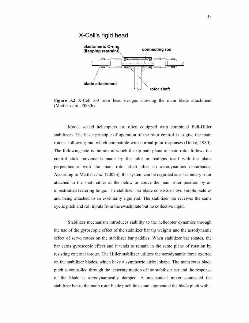
35
Figure 3.2 X-Cell .60 rotor head designs showing the main blade attachment (Mettler et al., 2002b)
Model scaled helicopters are often equipped with combined Bell-Hiller
stabilizers. The basic principle of operation of the rotor control is to give the main
rotor a following rate which compatible with normal pilot responses (Drake, 1980).
The following rate is the rate at which the tip path plane of main rotor follows the
control stick movements made by the pilot or realigns itself with the plane
perpendicular with the main rotor shaft after an aerodynamics disturbance.
According to Mettler et al. (2002b), this system can be regarded as a secondary rotor
attached to the shaft either at the below or above the main rotor position by an
unrestrained teetering hinge. The stabilizer bar blade consists of two simple paddles
and being attached to an essentially rigid rod. The stabilizer bar receives the same
cyclic pitch and roll inputs from the swashplate but no collective input.
Stabilizer mechanism introduces stability to the helicopter dynamics through
the use of the gyroscopic effect of the stabilizer bar tip weights and the aerodynamic
effect of servo rotors on the stabilizer bar paddles. When stabilizer bar rotates, the
bar earns gyroscopic effect and it tends to remain in the same plane of rotation by
resisting external torque. The Hiller stabilizer utilizes the aerodynamic force exerted
on the stabilizer blades, which have a symmetric airfoil shape. The main rotor blade
pitch is controlled through the teetering motion of the stabilizer bar and the response
of the blade is aerodynamically damped. A mechanical mixer connected the
stabilizer bar to the main rotor blade pitch links and augmented the blade pitch with a

36
component proportional to the stabilizer bar flapping angle (Mettler et al., 2002a).
Figure 3.3 shows the basic mechanical operation of stabilizer bar.
Figure 3.3 The stabilizer bar mechanical system operation in RC helicopter (Mettler et al., 2002a)
3.2 Helicopter Parameters
The helicopter parameters required to conduct the performance, stability and
control analysis were determined either from physical measurement, look-up table or
experimental test. Using the physical parameterization of air vehicle, it is hoped to
develop a simulation model capable of conducting frequency and time response
analyses. The physical helicopter parameters used for the model in research are given
in Table 3.1. Several parameters such as nominal main rotor speed, nomΩ , tail rotor
to main rotor gear ratio, Tn and engine shaft to main rotor gear ratio, esn could be
obtained from Thunder Tiger Corp. (2004).
3.2.1 Physical Measurement.
Measurements of those input variables from the UAV could be measured
from an arbitrary reference datum. The datum, located roughly at the unmodified
UAV center of gravity (CG), was designated as waterline (WL) zero and butt line

37
(BL) zero. The nose of the helicopter was designated as fuselage station (FS) zero
(McEwen, 1998). Additional measurement methods are presented in the following
sections.
Table 3.1 Parameters of Raptor .90 helicopter for simulation model Parameter Description
ρ = 1.225 kg/m3 Atmosphere density m = 7.70 kg Helicopter mass
Ixx = 0.192 kg m2 Rolling moment of inertia Iyy = 0.34 kg m2 Pitching moment of inertia Izz = 0.280 kg m2 Yawing moment of inertia Kβ = 54 Nm/rad Hub torsional stiffness
γfb = 0.8 Stabilizer bar Lock number Ωnom = 162 rad/s Nominal main rotor speed
RM = 0.775 m Main rotor radius RCR = 0.370 m Stabilizer bar radius cM = 0.058 m Main rotor chord cCR = 0.06 m Stabilizer bar chord
aM = 5.5 rad-1 Main rotor blade lift curve slope MDoC = 0.024 Main rotor blade zero lift drag coefficient
maxMTC = 0.00168 Main rotor max thrust coefficient
Iβ = 0.038 Main rotor blade flapping inertia RT = 0.13 m Tail rotor radius cT = 0.029 m Tail rotor chord aT = 5.0 rad-1 Tail rotor blade lift curve slope
TDoC = 0.024 Tail rotor blade zero lift drag coefficient
maxTTC = 0.0922 Tail rotor max thrust coefficient nT = 4.66 Gear ratio of tail rotor to main rotor nes = 9.0 Gear ratio of engine shaft to main rotor
trimrδ = 0.1 rad Tail rotor pitch trim offset
SV= 0.012 m2 Effective vertical fin area
HS =0.01 m2 Effective horizontal fin area VLC α = 2.0 rad-1 Vertical fin lift curve slope HLC α = 3.0 rad-1 Horizontal tail lift curve slope
FxS = 0.1 m2 Frontal fuselage drag area FyS = 0.22 m2 Side fuselage drag area FzS = 0.15 m2 Vertical fuselage drag area
hM = 0.235 m Main rotor hub height above CG lM = 0.015 m Main rotor hub behind CG lT = 0.91 m Tail rotor hub location behind CG hT = 0.08 m Tail rotor height above CG lH= 0.71 m Stabilizer location behind CG
kMR =0.3333 Amount of commanded swashplate tilt
kβ =1 Resulting control rotor plane tilt acting on the blade pitch
kCR =1.1429 Geometry coefficient of the mechanical linkage of control rotor and swashplate
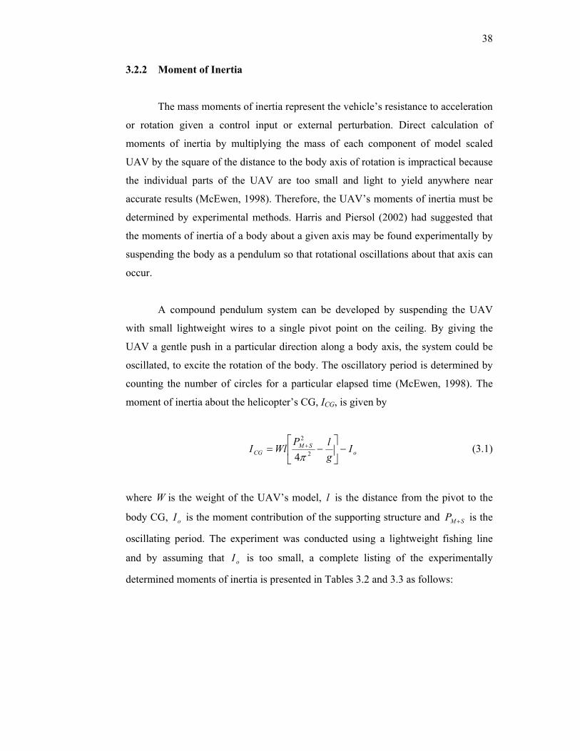
38
3.2.2 Moment of Inertia
The mass moments of inertia represent the vehicle’s resistance to acceleration
or rotation given a control input or external perturbation. Direct calculation of
moments of inertia by multiplying the mass of each component of model scaled
UAV by the square of the distance to the body axis of rotation is impractical because
the individual parts of the UAV are too small and light to yield anywhere near
accurate results (McEwen, 1998). Therefore, the UAV’s moments of inertia must be
determined by experimental methods. Harris and Piersol (2002) had suggested that
the moments of inertia of a body about a given axis may be found experimentally by
suspending the body as a pendulum so that rotational oscillations about that axis can
occur.
A compound pendulum system can be developed by suspending the UAV
with small lightweight wires to a single pivot point on the ceiling. By giving the
UAV a gentle push in a particular direction along a body axis, the system could be
oscillated, to excite the rotation of the body. The oscillatory period is determined by
counting the number of circles for a particular elapsed time (McEwen, 1998). The
moment of inertia about the helicopter’s CG, ICG, is given by
oSM
CG IglP
WlI −⎥⎦
⎤⎢⎣
⎡−= +
2
2
4π (3.1)
where W is the weight of the UAV’s model, l is the distance from the pivot to the
body CG, oI is the moment contribution of the supporting structure and SMP + is the
oscillating period. The experiment was conducted using a lightweight fishing line
and by assuming that oI is too small, a complete listing of the experimentally
determined moments of inertia is presented in Tables 3.2 and 3.3 as follows:
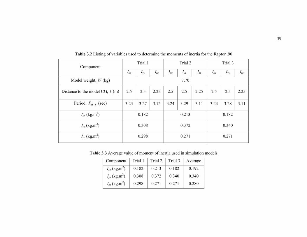
39
Table 3.2 Listing of variables used to determine the moments of inertia for the Raptor .90
Trial 1 Trial 2 Trial 3 Component
Ixx Iyy Izz Ixx Iyy Izz Ixx Iyy Izz
Model weight, W (kg) 7.70
Distance to the model CG, l (m) 2.5 2.5 2.25 2.5 2.5 2.25 2.5 2.5 2.25
Period, SMP + (sec) 3.23 3.27 3.12 3.24 3.29 3.11 3.23 3.28 3.11
Ixx (kg.m2) 0.182 0.213 0.182
Iyy (kg.m2) 0.308 0.372 0.340
Izz (kg.m2) 0.298 0.271 0.271
Table 3.3 Average value of moment of inertia used in simulation models
Component Trial 1 Trial 2 Trial 3 Average
Ixx (kg.m2) 0.182 0.213 0.182 0.192
Iyy (kg.m2) 0.308 0.372 0.340 0.340
Izz (kg.m2) 0.298 0.271 0.271 0.280

40
3.2.3 Rotor Flapping Moment
The rotor flapping moment is the mass moment of inertia of the blade about
the flapping hinge. The rotor flapping moment influences the rotor blade’s ability to
flap due to blade pitch changes caused by cyclic inputs. The flap moment of inertia is
defined by Padfield (1996) as
∫=R
drmrI0
2β (3.2)
where m is the specific mass of the blade mass distribution (kg/m), r is the radius of
the blade element (m) and R is the total blade radius (m). For the main and tail
rotors, the blade mass distribution was assumed uniform; therefore, the above
relation can be simplified as
3
3mRIβ = (3.3)
3.2.4 Aerodynamic Input
Several of the required inputs for the simulation model building were
unavailable neither by direct measurement nor experimentally. Several resources
were required to satisfy the required data input fields. Below is a listing of these
input data with a brief description, reasoning and reference source.
i. Forward Velocity
For hover analysis, forward velocity is equal to zero (no wind condition). If
performing an analysis for forward flight, UAV airspeed data is required in
order to get accurate results of simulations analysis. At present, no published
data exists for such vehicle. However this data could be obtained through a
simple method by determining the time to fly between two points of a known

41
distance apart, yielding an approximate velocity. But several assumptions had
to be made which is the maximum forward speed corresponds to an advance
ratio µ = 0.15 is considered as relatively low (Padfield, 1996) and permit
thrust perpendicular to the rotor disk assumption. The cross-coupling effects
in the rotor hub were also assumed to be neglected for model scaled
helicopter. This assumption further simplified the model development.
ii. Main and Tail Rotor Lift Curve Slopes
Exact airfoil data for Raptor .90 UAV was unavailable from the manufacturer
and time constrains limited wind tunnel testing. The lift curve slopes, ao of X-
Cell .60 main and tail rotors and as well as its stabilizer bar were determined
according to their aspect ratio (Nelson, 1998).
iii. Rotor Rotational Velocity
The rotational velocity of the main rotor system was determined using a RPM
checker. With the UAV in a normal hovering operation, the rotor rotational
velocity was recorded in revolutions per minute (rpm). The rotational velocity
of the tail rotor was determined by using the gearing ratio between the main
and tail rotors i.e. in the order of 1:4.66.
iv. Rotor Blade Airfoil
As stated before, the UAV airfoil data was unavailable. The Raptor .60 UAV
was assumed to have symmetrical NACA 0012 airfoils for main and tail
rotors and also the stabilizer bar.
v. Horizontal and Vertical Tail Coefficient of Lift Curve Slope
The expected values of empennage surface lift curve slope are dependent
upon the airfoil sections and their aspect ratios (Nelson, 1998). For flat plate,
representative values were plotted against effective aspect ratio ( eAR ). Using
the aspect ratio eAR of horizontal surface, the value of αLC was obtained.
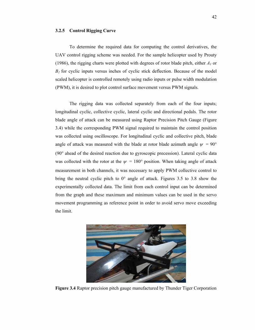
42
3.2.5 Control Rigging Curve
To determine the required data for computing the control derivatives, the
UAV control rigging scheme was needed. For the sample helicopter used by Prouty
(1986), the rigging charts were plotted with degrees of rotor blade pitch, either A1 or
B1 for cyclic inputs versus inches of cyclic stick deflection. Because of the model
scaled helicopter is controlled remotely using radio inputs or pulse width modulation
(PWM), it is desired to plot control surface movement versus PWM signals.
The rigging data was collected separately from each of the four inputs;
longitudinal cyclic, collective cyclic, lateral cyclic and directional pedals. The rotor
blade angle of attack can be measured using Raptor Precision Pitch Gauge (Figure
3.4) while the corresponding PWM signal required to maintain the control position
was collected using oscilloscope. For longitudinal cyclic and collective pitch, blade
angle of attack was measured with the blade at rotor blade azimuth angle ψ = 90°
(90° ahead of the desired reaction due to gyroscopic precession). Lateral cyclic data
was collected with the rotor at the ψ = 180° position. When taking angle of attack
measurement in both channels, it was necessary to apply PWM collective control to
bring the neutral cyclic pitch to 0° angle of attack. Figures 3.5 to 3.8 show the
experimentally collected data. The limit from each control input can be determined
from the graph and these maximum and minimum values can be used in the servo
movement programming as reference point in order to avoid servo move exceeding
the limit.
Figure 3.4 Raptor precision pitch gauge manufactured by Thunder Tiger Corporation
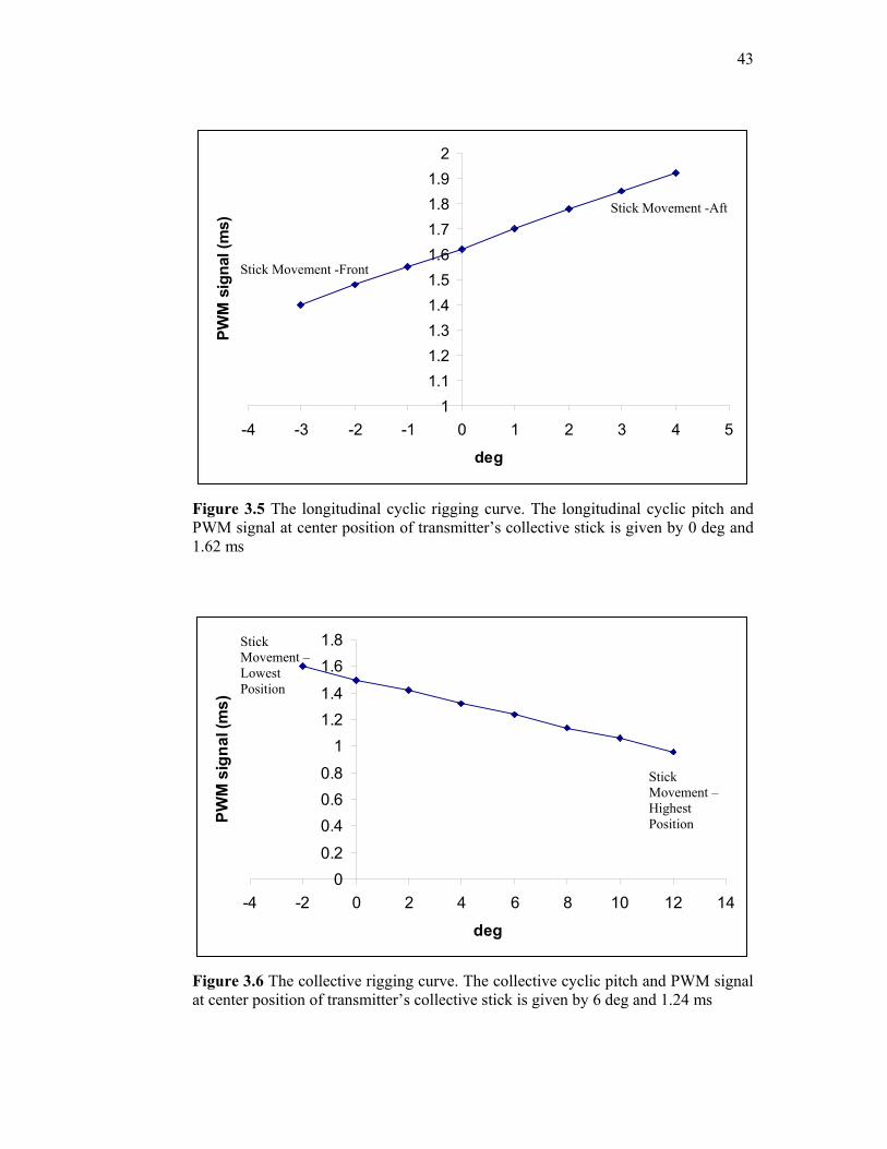
43
11.11.21.31.41.51.61.71.81.9
2
-4 -3 -2 -1 0 1 2 3 4 5
deg
PWM
sig
nal (
ms)
Figure 3.5 The longitudinal cyclic rigging curve. The longitudinal cyclic pitch and PWM signal at center position of transmitter’s collective stick is given by 0 deg and 1.62 ms
00.2
0.40.60.8
11.21.4
1.61.8
-4 -2 0 2 4 6 8 10 12 14
deg
PWM
sig
nal (
ms)
Figure 3.6 The collective rigging curve. The collective cyclic pitch and PWM signal at center position of transmitter’s collective stick is given by 6 deg and 1.24 ms
Stick Movement – Lowest Position
Stick Movement – Highest Position
Stick Movement -Front
Stick Movement -Aft

44
00.20.40.60.8
11.21.41.61.8
2
-6 -5 -4 -3 -2 -1 0 1 2 3 4 5 6
deg
PWM
sig
nal (
ms)
Figure 3.7 The lateral cyclic rigging curve. The lateral cyclic pitch and PWM signal at center position of transmitter’s lateral stick is given by -1 deg and 1.48 ms
00.20.40.60.8
11.21.41.61.8
2
-8 -7 -6 -5 -4 -3 -2 -1 0 1 2 3 4 5 6 7 8
deg
PWM
sig
nal (
ms)
Figure 3.8 The directional control rigging curve. The tail rotor pitch and PWM signal at center position of transmitter’s rudder stick is given by -2 deg and 1.58 ms
Rudder Stick left
Rudder Stick - Right
Stick Movement -Right
Stick Movement -Left

45
3.3 Helicopter Model
Helicopter dynamics obey the Newton-Euler equation for rigid body in
translational and rotational motions. The helicopter dynamics can be studied by
employing lumped parameter approach which indicates that the helicopter as the
composition of following components; main rotor, tail rotor, fuselage, horizontal bar
and vertical bar (Shim, 2000). Figure 3.9 illustrates typical arrangement of
component forces and moments generation in helicopter simulation model.
Figure 3.9 Typical arrangement of component forces and moments generation in
helicopter simulation model (Padfield, 1996)
The general nonlinear equations of motion of an helicopter take the form of
( , , )x F x u t= (3.4)
where the state vector x has components from the fuselage fx , rotors rx ,
engine/rotorspeed px , and control actuation cx sub-systems. The corresponding state
vectors were given in equations 3.5 to 3.9, where u, v and w are the translational

46
velocities along the three orthogonal directions of the fuselage fixed axes system as
derived by Padfield (1996). p, q and r are the angular velocities about the x-, y- and
z- axes and θ , φ and Ψ are the Euler angles defining the orientation of the body
axes relative to the earth. In equation 3.7, the 0a is called rotor blade coning angle,
1sa is called the longitudinal flapping with respect to a plane perpendicular to the
shaft and defined as positive when the blade flaps down at the tail and up at the nose,
1sb is called the lateral flapping defined as positive when the blade flaps down on the
advancing side and up on the retreating side, 0λ , 1cλ and 1sλ are the rotor uniform
and first harmonic inflow velocities in hub/shaft axes. Ω is the main rotor speed and
eQ the engine torque. The control actuation vector has four components consisting of
main rotor collective colδ , longitudinal cyclic lonδ , lateral cyclic latδ and tail rotor
collective pedδ .
, , ,f r p cx x x x x= (3.5)
, , , , , , ,fx u w q v p rθ φ= (3.6)
0 0 1 1, , , , ,r c sx a a b λ λ λ= (3.7)
, ,p e ex Q Q= Ω (3.8)
, , ,c col lon ped latx δ δ δ δ= (3.9)
The helicopter rigid body equations of motion are given by Newton-Euler
equations as follows. The equations of motion were described in nonlinear form with
only considering fuselage state vector.
Force equations:
( ) sina
Xu wq vr gM
θ= − − + − (3.10)
( ) cos sina
Yv ur wp gM
θ φ= − − + + (3.11)

47
( ) cos cosa
Zw vp uq gM
θ φ= − − + + (3.12)
Moment equations:
( ) ( )xx yy zz xzI p I I qr I r pq L= − + + + (3.13)
( ) ( )2 2yy zz xx xzI q I I rp I r p M= − + − + (3.14)
( ) ( )zz xx yy xzI r I I pq I p qr N= − + − + (3.15)
Kinematic equations:
sin tan cos tanp q rφ φ θ φ θ= + + (3.16)
cos sinq rθ φ φ= − (3.17)
sin sec cos secq rφ θ φ θΨ = + (3.18)
The equation of motion can be expanded by summing the forces and
moments generated from the components such as main rotor, tail rotor, fuselage,
horizontal stabilizer and vertical stabilizer. The free body diagram of an helicopter in
body axes is shown in Figure 3.10. The forces terms in the x, y and z directions are
represented by X, Y and Z while the moment terms in roll, pitch and yaw directions
are represented by R, M and N respectively. The subscripts M, T, F, H and V
represented main rotor, tail rotor, fuselage, horizontal stabilizer and vertical
stabilizer.

48
Figure 3.10 Free body diagram of scaled model helicopter in body coordinate system (Shim, 2000)
The cross products of inertia can be neglected in the analysis and the
expended equations of motions were shown in equations 3.19 to 3.24. The
formulation of each force and moment terms can be calculated using methods outline
by Prouty (1995) and Padfield (1996).
( ) [ ]1 sinM T H V Fa
u wq vr X X X X X gM
θ= − − + + + + + − (3.19)
( ) [ ]1 cos sinM T V Fa
v ur wp Y Y Y Y gM
θ φ= − − + + + + + (3.20)
( ) [ ]1 cos cosM T H V Fa
w vp uq Z Z Z Z Z gM
θ φ= − − + + + + + + (3.21)
( ) [ ]1 1yy zz M M M M M T T V V F F F
xx xx
p I I qr R Y h Z y Y h Y h Y h RI I
= − + + + + + + + (3.22)

49
( )1 1 M M M M M T T T T T H Hzz xx
H H V V Fyy yy
M X h Z l M X h Z h X hq I I rp
Z l X h MI I− + + − + −⎡ ⎤
= − + ⎢ ⎥+ − +⎣ ⎦
(3.23)
( ) [ ]1 1xx yy M M M T T V V F F F
zz zz
r I I pq N Y l Y l Y l N Y lI I
= − + − − − + − (3.24)
The aerodynamic forces can be described in the wind frame since all of these
forces depend on the velocity relative to the surrounding air mass. This wind frame is
as well fixed to the aircraft, but the x-axis is now oriented along the velocity vector V
of the vehicle relative to the atmosphere. The z-axis lies again in the plane of
symmetry and the y-axis is perpendicular to both. The origin is again located at the
CG of the aircraft. The wind frame and notations for an helicopter in forward flight
are shown in Figure 3.11.
Figure 3.11 Wind axes of a helicopter in forward flight
3.4 Linearized Model
The nonlinear model (equations 3.19 to 3.24) for hover is valuable for the
nonlinear simulation model and it can be further simplified to obtain the linear
model. A linear dynamic model for helicopter is needed for the stability analysis and
50
the design of linear feedback control system. Aerodynamic effects can be assumed to
be linear functions of disturbances and the values of linear and angular velocity
perturbations are usually small for many cases.
The linearization process assumes small disturbances, so only the first-order
terms are kept, while squares and products are assumed to be negligible. For a
steady-state flight condition all disturbances are set equal to zero. Linear relations to
eliminate reference forces and moments acting on the vehicle in this trimmed flight
condition are obtained. Then the classic assumption of linear aerodynamic theory
allows us to express aerodynamic forces in terms of stability derivatives.
The system and control matrices F and G for hover listed in Appendix A
show all of the important gravitational terms that can be obtained analytically and
partial derivatives arising from aerodynamic forces and moments necessary to
describe the linear set of equations for an helicopter. The linear, first-order set of
differential equations is given in the form of equation 3.25 and the detailed
derivation of partial derivatives is given in Prouty (1986) and Padfield (1996).
.x = F x + G uδ (3.25)
The system matrix F includes derivatives due to small perturbations of system states
while the control matrix G represents the derivatives due to small perturbations of
control inputs. In sic degrees of freedom form, the motion states and control are,
x , , , , , , , u w q v p rθ φ= (3.26)
where u, v and w are the translational velocities along the three orthogonal directions
of the fuselage fixed axes system. p, q and r are the angular velocities about the x-, y-
and z- axes and θ , φ and ψ are the Euler angles defining the orientation of the body
axes relative to the earth. The control vector has four components consisting of the
main rotor collective, tail rotor collective, lateral cyclic and longitudinal cyclic.
u 1 1 , , , O OT A Bθ θ= (3.27)

51
It can be seen that the throttle is not considered to be a control input. For a
wide range of flight conditions, the rotational speed of the rotor does not change, and
a variation of throttle is made only to adjust power for keeping some desired
rotational rotor speed constant. One way to obtain the force and moment derivatives
is to sequentially perturb the states and control inputs, positively and negatively from
trim values by some small amount ∆. Then the forces and moments due to both
perturbed conditions are computed, and the derivatives can be obtained by using the
following equation.
( ) ( )0 0
2u
X u u X u uXXu u
δδ
+ ∆ − − ∆= ≅
∆ (3.28)
The force X and the state u in this equation represent all the forces, moments,
states and control inputs in the equations of motion. This approach is used in the later
described simulation routine to compute the linear system matrices for any desired
trimmed flight condition. Linear system analysis is very useful and convenient to
examine eigenvalues or eigenvectors, system responses to step inputs, frequency
response and other stability characteristics of a dynamic system.
3.5 Main Rotor Forces and Moments
The main rotor is the primary component of helicopter dynamics and it’s
responsible for producing vertical thrust vector and an induced velocity field.
Assumptions such as the inflow are steady and uniform distribution is made in main
rotor thrust calculation. The simplest theory that allows the relationship between
rotor thrust, torque and the inflow ratio to be derived is commonly known as the
momentum theory which utilizing the conservation laws of mass, momentum and
energy (Padfield, 1996). Figure 3.12 illustrates the flow states for the rotor in axial
motion when the resultant flow is always normal to the rotor disc corresponding to
hover, climbing or descending flight. Referring to Figure 3.12, T is the rotor thrust,

52
v is the velocity at various stations in the stream tube, iv is the induced velocity at
the disc, cV is the climb velocity and dV is the rotor descent velocity.
Figure 3.12 Rotor flow states in axial motion. (a) Hover condition (b) Climb condition and (c) Descent condition (Padfield, 1996)
The mass flow through the rotor in hover and climb states can be shown as in
equation 3.29 below with m is the mass flow rate (constant at each station) and dA
the rotor disc area:
( )d c im A V vρ= + (3.29)
The rate of change of momentum between the undisturbed upstream and the far wake
conditions can be equated to the rotor loading to give
( )c i c iT m V v mV mv∞ ∞= + − = (3.30)
where iv ∞ is the induced flow in the fully developed wake.
The change in the kinetic energy of the flow can be related to the work done
by the rotor (actuator disc) as follow:

53
( ) ( ) ( )2 2 21 1 1 22 2 2c i c i c c i iT V v m V v mV m V v v∞ ∞ ∞ ∞+ = + − = + (3.31)
Note that the induced velocity in the far wake is found to be accelerated to twice the
rotor inflow and can be written as
2i iv v∞ = (3.32)
The expression for the rotor thrust can now be written directly in terms of the
conditions at the rotor disc as follow:
( )2 d c i iT A V v vρ= + (3.33)
The induced velocity can be also written in normalized form as inflow ratio, iλ :
ii
M
vR
λ =Ω
(3.34)
The hover induced velocity (with 0cV = ) in term of the rotor thrust coefficient, TC is
described in the equation below:
2hoverid
TvAρ
⎛ ⎞= ⎜ ⎟
⎝ ⎠ or
2T
ihCλ ⎛ ⎞= ⎜ ⎟
⎝ ⎠ (3.35)
The inflow in the climb situation can be written as:
( )2T
ic i
Cλµ λ
=+
(3.36)
or derived from the positive solution of the quadratic equation
( )2ih c i iλ µ λ λ= + (3.37)

54
as
22
2 2c c
i ihµ µλ λ
⎡ ⎤⎛ ⎞= − + +⎢ ⎥⎜ ⎟⎝ ⎠⎢ ⎥⎣ ⎦
(3.38)
where
cc
M
VR
µ =Ω
(3.39)
The case of vertical descent condition (where cV < 0) is more complicated
since it has similarity to a windmill that extracts energy from the air (Figure 3.12).
This rotor condition is called the windmill brake state and the work done by the rotor
on the air is now negative and following a similar analysis for climb, the rotor thrust
can be written as
( )2 d d iT A V vρ= − (3.40)
22
2 2d d
i ihµ µλ λ
⎡ ⎤⎛ ⎞= − −⎢ ⎥⎜ ⎟⎝ ⎠⎢ ⎥⎣ ⎦
(3.41)
where
dd
M
VR
µ =Ω
(3.42)
The physical solutions for equations 3.38 and 3.41 are plotted in Figure 3.13
to show the induced velocity variations for both the vertical climb and descent
situations of the Raptor .90. It is seen that as the climb velocity increased ( c
ih
µλ >
0), the induced velocity at the rotor decreased. This particular region is called the
normal working state of rotor. Leishman (2002) and Padfield (1996) had stated that
for cases whenever descent velocity is in the range of -2 < c
ih
µλ < 0, the simple
momentum theory is invalid because the velocity at any plane through the rotor
slipstream can be either upward or downward. A more complicated turbulent flow

55
pattern may exist at the rotor and the momentum theory simply cannot be used since
there was no control volume established. Padfield (1996) and Leishman (2002) had
reported that some experimental estimates can be used to find approximation for the
inflow in this range using the work carried out by Young (1978) and Johnson (1980).
Young’s approximations take the forms of
1 ci ih
ih
µλ λλ
⎛ ⎞= −⎜ ⎟
⎝ ⎠ for 0 ≥ c
ih
µλ ≥ -1.5 (3.43)
and
7 3 ci ih
ih
µλ λλ
⎛ ⎞= +⎜ ⎟
⎝ ⎠ for -1.5 > c
ih
µλ ≥ -2 (3.44)
0
0.5
1
1.5
2
2.5
3
-5 -4 -3 -2 -1 0 1 2 3
Climb Velocity Ratio
Inflo
w R
atio
µc/λih
λ i/λ ih
ClimbDescent
Momentum Theory Invalid
normal helicopter state
vortex ring state
Young's approximation
Figure 3.13 Induced velocity variation as a function of climb and descent velocities based on the simple momentum theory for Raptor .90
The computations of thrust coefficient and inflow ratio as a function of
airspeed, rotor speed and collective setting were accomplished using the momentum
theory based iterative scheme of Padfield (1996). The blades used for both Excel
0.60 and Raptor 0.90 have no twist. The influence of the cyclic and the roll rate on
the thrust is neglected for advanced ratio of µ < 0.15. According to Padfield (1996),

56
the maximum forward speed corresponds to advance ratio µ = 0.15 (20 m/s) is
considered as relatively low and permits thrust perpendicular to the rotor disk
assumption. An empirically determined maximum thrust coefficient can be used
since the momentum theory does not take into account the effect of blade stall. The
thrust coefficient is given by
( )2 2T
TCR Rρ π
=Ω
(3.45)
where T is the main rotor thrust. The induced velocity and the inflow ratio at hover
trim condition can be found using the equations 3.46 and 3.47 respectively. tipMV in
the equation 3.47 is the tip speed of helicopter main rotor.
22iM
mgVRρπ
= (3.46)
i ii tip
M M M
V VV R
λ = =Ω
(3.47)
Then the following system of equations (3.48) – (3.55) can be solved iteratively:
( )
0 2202
T
w z
Cλη µ λ µ
=+ −
(3.48)
20
01
2 3 2 2ideal zMT
aC µ λσ µθ⎛ ⎞⎛ ⎞ −
= + +⎜ ⎟⎜ ⎟⎝ ⎠⎝ ⎠
(3.49)
idealTC if max
TC− ≤ idealTC ≤ max
TC
TC = maxTC− if ideal
TC < maxTC−
maxTC if max
TC < idealTC
(3.50)
( )
maxmax
2 2TM M
TCR Rρ π
=Ω
(3.51)
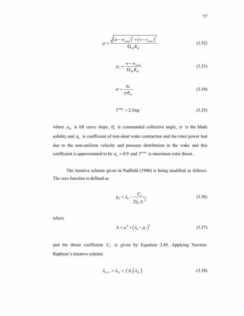
57
( ) ( )2 2wind wind
M M
u w v vR
µ− + −
=Ω
(3.52)
windz
M M
w wR
µ −=
Ω (3.53)
M
bcR
σπ
= (3.54)
max 2.5T mg= (3.55)
where Ma is lift curve slope, 0θ is commanded collective angle, σ is the blade
solidity and wη is coefficient of non-ideal wake contraction and the rotor power lost
due to the non-uniform velocity and pressure distribution in the wake and this
coefficient is approximated to be 0.9wη = and maxT is maximum rotor thrust.
The iterative scheme given in Padfield (1996) is being modified as follows.
The zero function is defined as
0 0 122
T
w
Cg λη
= −Λ
(3.56)
where
( )220 zµ λ µΛ = + − (3.57)
and the thrust coefficient TC is given by Equation 3.49. Applying Newton-
Raphson’s iterative scheme:
( )0 1 0 0j j j j jf hλ λ λ+ = + (3.58)
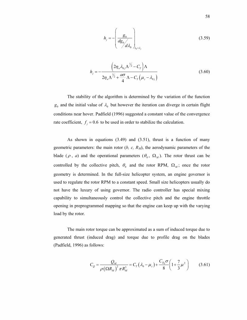
58
0
0
0
0j
jgh dgd
λ λλ
=
⎛ ⎞⎜ ⎟
= −⎜ ⎟⎜ ⎟⎝ ⎠
(3.59)
( )( )
12
0
32
0
2
24
w j T
j
w T z j
Ch a C
η λ
ση µ λ
Λ − Λ= −
Λ + Λ − − (3.60)
The stability of the algorithm is determined by the variation of the function
0g and the initial value of 0λ but however the iteration can diverge in certain flight
conditions near hover. Padfield (1996) suggested a constant value of the convergence
rate coefficient, 0.6jf = to be used in order to stabilize the calculation.
As shown in equations (3.49) and (3.51), thrust is a function of many
geometric parameters: the main rotor (b, c, RM), the aerodynamic parameters of the
blade ( ρ , a) and the operational parameters ( 0θ , MΩ ). The rotor thrust can be
controlled by the collective pitch, 0θ and the rotor RPM, MΩ ; once the rotor
geometry is determined. In the full-size helicopter system, an engine governor is
used to regulate the rotor RPM to a constant speed. Small size helicopters usually do
not have the luxury of using governor. The radio controller has special mixing
capability to simultaneously control the collective pitch and the engine throttle
opening in preprogrammed mapping so that the engine can keep up with the varying
load by the rotor.
The main rotor torque can be approximated as a sum of induced torque due to
generated thrust (induced drag) and torque due to profile drag on the blades
(Padfield, 1996) as follows:
( )
( ) 0 202 3
718 3DM
Q T zM M
CQC CR R
σλ µ µ
ρ π⎛ ⎞= = − + +⎜ ⎟⎝ ⎠Ω
(3.61)

59
where QC is the torque coefficient and 0DC is the profile drag coefficient of the main
rotor blade. The profile drag is not significantly affected by the changes in the
collective setting.
In order to gain some insight from the very complicated thrust equation, the
values evaluated were plotted using the quantities of Raptor 0.90. Under forward
flight conditions, the rotor moves through the air with an edgewise component of
velocity that is parallel to the plane of the rotor disk. In Figure 3.14, the inflow ratio
is plotted versus freestream velocity ratio for various disk incidence angles. It can be
seen that the inflow component is decreasing as the freestream velocity increase for
various incidence angle. Note that, the inflow ratio for positive incidence angle
(helicopter nose up) is decreasing as the incidence angle increase. In Figure 3.15, the
thrust calculation is plotted versus forward velocity and it appeared that as the
forward velocity increased, the value of thrust decreased for positive disc incidence
angle and this calculation hold true for 0–20 m/s forward velocity (Leishman, 2002).
The rotor thrust is found to increase as velocity increase for incidence angle 8° to -5°
which indicate that the rotor generated extra lift during forward flight and this effect
must be compensated by the pilot reducing the throttle in order to avoid helicopter
from climbing.
0
0.2
0.4
0.6
0.8
1
1.2
0 1 2 3 4 5
α=-5
α=0
α=1
α=3
α=8
α=20
Freestream velocity ratio, V/λh
Inflo
w R
atio
, λ0j/λ
h
Figure 3.14 Inflow solutions for Raptor .90 from momentum theory
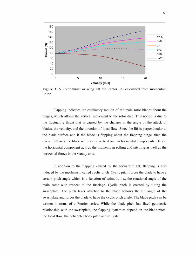
60
0
20
40
60
80
100
120
140
160
180
0 5 10 15 20Velocity (m/s)
Thru
st (N
)
α=-5α=0α=1α=3α=8α=20
Figure 3.15 Rotor thrust or wing lift for Raptor .90 calculated from momentum theory
Flapping indicates the oscillatory motion of the main rotor blades about the
hinges, which allows the vertical movement to the rotor disc. This notion is due to
the fluctuating thrust that is caused by the changes in the angle of the attack of
blades, the velocity, and the direction of local flow. Since the lift is perpendicular to
the blade surface and if the blade is flapping about the flapping hinge, then the
overall lift over the blade will have a vertical and an horizontal components. Hence,
the horizontal component acts as the moments in rolling and pitching as well as the
horizontal forces in the x and y axis.
In addition to the flapping caused by the forward flight, flapping is also
induced by the mechanism called cyclic pitch. Cyclic pitch forces the blade to have a
certain pitch angle which is a function of azimuth, i.e., the rotational angle of the
main rotor with respect to the fuselage. Cyclic pitch is created by tilting the
swashplate. The pitch lever attached to the blade follows the tilt angle of the
swashplate and forces the blade to have the cyclic pitch angle. The blade pitch can be
written in terms of a Fourier series. While the blade pitch has fixed geometric
relationship with the swashplate, the flapping dynamics depend on the blade pitch,
the local flow, the helicopter body pitch and roll rate.
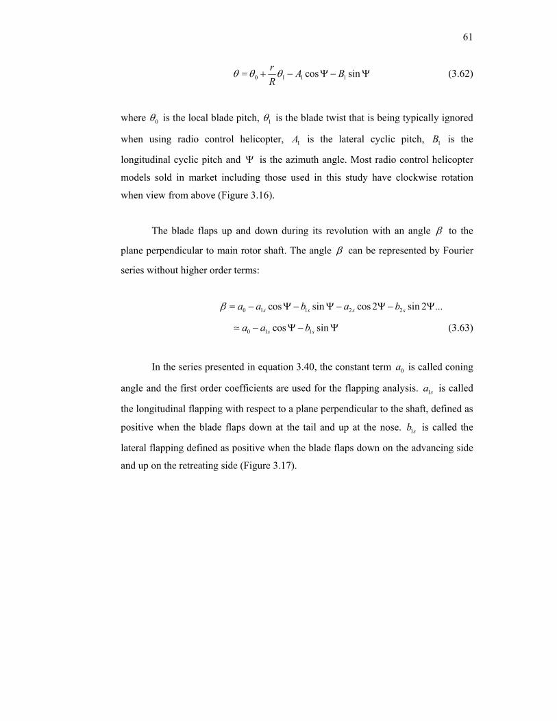
61
0 1 1 1cos sinr A BR
θ θ θ= + − Ψ − Ψ (3.62)
where 0θ is the local blade pitch, 1θ is the blade twist that is being typically ignored
when using radio control helicopter, 1A is the lateral cyclic pitch, 1B is the
longitudinal cyclic pitch and Ψ is the azimuth angle. Most radio control helicopter
models sold in market including those used in this study have clockwise rotation
when view from above (Figure 3.16).
The blade flaps up and down during its revolution with an angle β to the
plane perpendicular to main rotor shaft. The angle β can be represented by Fourier
series without higher order terms:
0 1 1 2 2cos sin cos 2 sin 2 ...s s s sa a b a bβ = − Ψ − Ψ − Ψ − Ψ
0 1 1cos sins sa a b− Ψ − Ψ (3.63)
In the series presented in equation 3.40, the constant term 0a is called coning
angle and the first order coefficients are used for the flapping analysis. 1sa is called
the longitudinal flapping with respect to a plane perpendicular to the shaft, defined as
positive when the blade flaps down at the tail and up at the nose. 1sb is called the
lateral flapping defined as positive when the blade flaps down on the advancing side
and up on the retreating side (Figure 3.17).

62
Figure 3.16 Azimuth angle reference point for clockwise rotor rotation viewed from above used mainly in most remote control helicopter manufactured outside US (Shim, 2000)
Figure 3.17 Rotor swashplate and flapping angles relationship (Shim, 2000)

63
The flapping effect describing the change of tip path plane (TPP) tilt of the
main rotor due to lateral and longitudinal velocities is dependent on the thrust and the
induced velocities respectively. The equation for the lateral tilt derivative can be
found in Prouty (1986) to be
1 822
s T Tdb C Cdv R aσ
⎛ ⎞= − +⎜ ⎟⎜ ⎟Ω ⎝ ⎠
(3.64)
where /bc Rσ π= is the rotor solidity and by assuming equal effects on lateral and
longitudinal motion, the longitudinal derivative is given as
1 1
b b
da dbdu dv
= (3.65)
The assumption of constant derivatives in hover is true as long as uniform
inflow is assumed. For fast forward flight, non-uniform inflow becomes necessary
and this assumption is only an approximation. An empirical variable wakef such as
been used on full size helicopter is introduced to give a more accurate estimation
considering low or high-speed effects on those derivatives as described in Heffley
and Mnich (1986) and Munzinger (1998). This variable will be used in the dynamic
rotor equations. The empirical value for wakef dependants on flight speed and can be
chosen based on experience or experimental data, if available and necessary. For the
Raptor .90 flying at low speed, this variable will always be equal to 1.
With respect to the cross-coupling of longitudinal and lateral TPP tilt, the two
already mentioned components needed to be considered are the mechanical linkages
from the swashplate and the control rotor to the main rotor. These linkages cause an
additional flap angle due to a commanded blade pitch change. The geometry of these
linkages and the rotor hub design result in an off-axis motion. From Figure 3.18, 3δ ,
the angle between the flap hinge axis and an imaginary line drawn from the hinge to
the pitch horn of the main rotor blade is found. Hence, the cross-coupling coefficient
is obtained using equation 3.66. This coefficient also describes the mechanical

64
feedback from flap angle to blade pitch; automatically decreasing pitch for an
increasing flap angle.
1 3tanK δ= (3.66)
Figure 3.18 Cross coupling due to the 3δ angle (Bramwell et al., 2001)
The second effect of cross-coupling can be derived from the fact that a
flapping hinge with an offset from the axis of rotation also changes the natural
frequency of the dynamic system (Munzinger, 1998). With the ratio computed by the
hinge offset MRe relative to the main rotor radius MRR , this coefficient can be written
as
234
MR M
MR f
eKR
Ω=
Ω (3.67)
where MΩ is the rotor rotational speed and Ωf is given by equation 3.68 as follows:
8116 3
MR MRf
MR
eR
γ ⎛ ⎞ΩΩ = +⎜ ⎟
⎝ ⎠ (3.68)
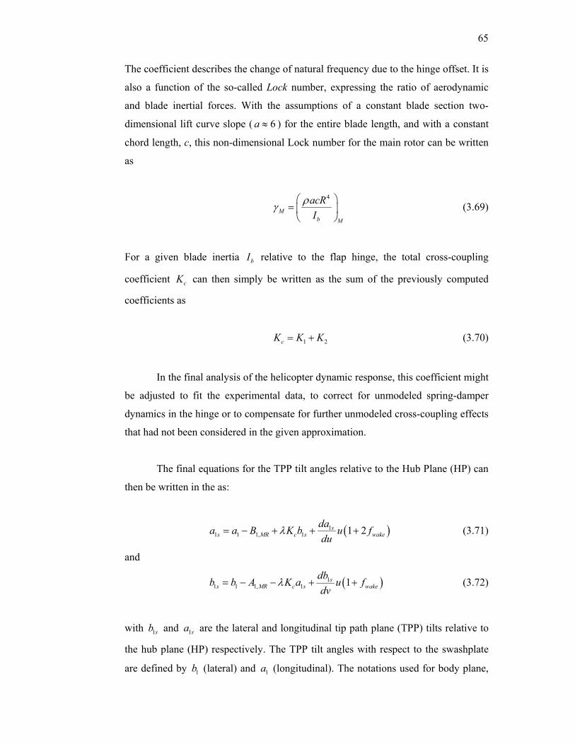
65
The coefficient describes the change of natural frequency due to the hinge offset. It is
also a function of the so-called Lock number, expressing the ratio of aerodynamic
and blade inertial forces. With the assumptions of a constant blade section two-
dimensional lift curve slope ( 6a ≈ ) for the entire blade length, and with a constant
chord length, c, this non-dimensional Lock number for the main rotor can be written
as
4
Mb M
acRI
ργ⎛ ⎞
= ⎜ ⎟⎝ ⎠
(3.69)
For a given blade inertia bI relative to the flap hinge, the total cross-coupling
coefficient cK can then simply be written as the sum of the previously computed
coefficients as
1 2cK K K= + (3.70)
In the final analysis of the helicopter dynamic response, this coefficient might
be adjusted to fit the experimental data, to correct for unmodeled spring-damper
dynamics in the hinge or to compensate for further unmodeled cross-coupling effects
that had not been considered in the given approximation.
The final equations for the TPP tilt angles relative to the Hub Plane (HP) can
then be written in the as:
( )11 1 1, 1 1 2s
s MR c s wakedaa a B K b u fdu
λ= − + + + (3.71)
and
( )11 1 1, 1 1s
s MR c s wakedbb b A K a u fdv
λ= − − + + (3.72)
with 1sb and 1sa are the lateral and longitudinal tip path plane (TPP) tilts relative to
the hub plane (HP) respectively. The TPP tilt angles with respect to the swashplate
are defined by 1b (lateral) and 1a (longitudinal). The notations used for body plane,

66
tip path plane and hub plane are given in Figure 3.19. The influence of the cross-
coupling is dependent on the direction of rotor rotation. Therefore the directional
parameter needs to be considered in those terms. The inputs applied to the blade
pitch angle are given by lateral cyclic input, 1,MRA and longitudinal cyclic, 1,MRB .
These are the resulting blade pitch changes commanded by the pilot stick inputs (RC
transmitter), transmitted by the swashplate tilt and the mechanical linkage from
swashplate to the pitch horn. The cross-coupling in equations 3.71 and 3.72
influences the TPP tilt and also depends on the direction of rotor rotation. The lateral
and longitudinal swashplate tilts 1,SPA and 1,SPB commanded by the pilot are
distributed by mechanical linkages to the control rotor as well as directly to the main
rotor. The largest portion is fed through the control rotor and the resulting tilt of the
control rotor plane due to control rotor blade pitch changes, commands the main
rotor blade pitch through mechanical linkages. The resulting main rotor input is
independent on the direction of rotor rotation and thus could be defined as follows:
1, 1, ,MR MR SP s CRA k A kβ β= + (3.73)
and
1, 1, ,MR MR SP c CRB k B kβ β= + (3.74)
The coefficients MRk and kβ prescribe the amount of commanded swashplate tilt and
the resulting control rotor plane tilt finally acting on the main rotor blade pitch. The
additional state coefficients ,s CRβ and ,c CRβ describe the lateral and longitudinal TPP
tilt of the control rotor with respect to the HP. The equations of motion for the
control rotor are given in Section 3.5.2, the coefficients MRk and kβ are found by
measuring linkage lengths and angles of pitch changes due to a swashplate tilt and
the equation can be found in Appendix B.

67
Figure 3.19 Hub plane, tip path plane and body axes notations (Munzinger, 1998)
The collective input commanded by the pilot is fed directly to the main rotor
and therefore does not appear explicitly in the main rotor flapping equations. It is
assumed that the collective pitch directly influences the induced velocity through the
rotor disk and hence the thrust. For an equally distributed change of blade pitch over
the rotor azimuth due to collective stick input and the resulting swashplate
displacement, it can also be assumed that effects on lateral and longitudinal TPP tilts
are small and will be neglected (Munzinger, 1998). The final equations of main rotor
flapping motion in the rotating rotor frame relative to the swashplate can be written
in the simplified forms as:
1 1in offa a b qω λω= − − − (3.75)
and
1 1in offb b a pω λω= − − − (3.76)
The simplified flap rate coefficients inω and offω for in- and off-axis changes of the
flap angle can be computed with no flap-cross-coupling as:

68
0off
in f
ω
ω
=
= Ω (3.77)
or with the flap-cross coupling as:
2
1
Moff
M
f
Min off
f
ω
ω ω
Ω=
⎛ ⎞Ω+ ⎜ ⎟⎜ ⎟Ω⎝ ⎠
Ω=
Ω
(3.78)
Equation 3.78 gives an approximation for the effect of cross-coupling in the flap
rates and also in the flap angles. Heffley and Mnich (1986) had mentioned that a
better fit to experimental data might be obtained by neglecting the rate-cross-
coupling in the simulation.
With respect to the hinge offset, the effect of pilot cyclic input should also be
considered. A pilot cyclic input causes a change in the flapping and hence in the TPP
tilt angles. Thus causes a change in the aerodynamic blade moment acting on the
helicopter in the case of a nonzero hinge offset only. For no hinge offset the blades
are free to flap and no moments are transferred to the rotor hub. Raptor .90 helicopter
model has no hinge offset arrangement and the only rotor moments acting on the
helicopter with no hinge offset ( / 0MR MRe R = ) are generated by the rotor forces and
the moment arm given the distance from the hub to the helicopter center of gravity
(CG). An approximation for the in-axis blade moment due to cyclic inputs with a
hinge offset is given by the equation 3.79 (Prouty, 1986). Equation 3.80 represents
the aerodynamic and inertial flap-cross-coupling moment including a hinge offset.
The computed moments can be written in the body-fixed frame as
2 2
1 1 12MR
M tipMR
edM dL BacR VdB dA R
ρ= = (3.79)
( )22
1 1
34
M M MR
s s MR
BacR R edM dLda db R
ρλ
γ
⎛ ⎞Ω⎜ ⎟= =⎜ ⎟⎝ ⎠
(3.80)

69
The main rotor dynamics are usually very fast compared to the rigid body
dynamics of the helicopter (Mettler et al., 2002b). Therefore a quasi-steady-state
model of the main rotor can be used to describe the dynamics of the body-rotor
dynamics. This approach is also very useful since additional dynamics result in
additional states that need to be integrated. The DOFs to be added are the
longitudinal and lateral tilt angles of the main rotor TPP and also of the control rotor
TPP. This would result in a model extension from 6 (8 states) to 10 DOF (12 states).
To avoid the 10 DOF model, the steady-state model for the main rotor will be
used to represent the rotating subsystem dynamics. Using this approximation, the
flight dynamics and control characteristics will still remain accurate (Munzinger,
1998). Nevertheless the two control rotor states (8 DOF with 10 states) are added to
the equations of rigid body motion. The control rotor is treated like a smaller rotor
with only a limited blade profile. The following section gives the quasi steady-state
equations for the main rotor derived from the previous dynamic equations.
3.5.1 Quasi Steady State Equations for Main Rotor Dynamics
For the valid steady-state blade motion it is assumed that the desired
orientation of the TPP is reached instantaneously. Prouty (1986) had reported that the
transient flap motion is a highly damped oscillation with an approximate time
constant 16 /τ γ≈ . The resulting time-to-half amplitude, 1/ 2 0.693t τ= , typically
corresponds to 90° of the rotor azimuth, and the transient response dies out after less
than one revolution of the main rotor. Steady-state equations are obtained by the
necessary conditions for steady-state.
1
1
0
0
a
b
=
= (3.81)

70
Solving equations 3.71 and 3.72 for 1a and 1b and substituting these values into
equations 3.75 and 3.76, the steady-state equations for the main rotor TPP angles
relative to the HP are:
( ) ( )( )1 1 3 4 2 4 32 21 2
1s in off in offa T q T T T p T T
T Tω λω ω λω= + − + − −
+ (3.82)
and
( )1 4 3 1 21
1s in off sb p T T a T
Tω λω= − − − (3.83)
The terms 1T , 2T , 3T and 4T are given by the equations 3.84-3.87 respectively . Note
that cK is the total cross coupling coefficient due to hinge offset.
( )1 in off cT Kω ω= − − (3.84)
( )2 in c offT Kλ ω ω= − + (3.85)
( )13 1, 1 2s
MR wakedaT B u fdu
⎛ ⎞= − +⎜ ⎟⎝ ⎠
(3.86)
( )14 1, 1s
MR wakedbT A v fdv
⎛ ⎞= + +⎜ ⎟⎝ ⎠
(3.87)
Equations 3.82 and 3.83 are then used to compute the TPP tilt angles 1sa and 1sb
relative to the main rotor HP. The assumption of a thrust vector perpendicular to the
TPP is used to transform the thrust components into the body-fixed frame by
( )1sinM s sX T a i= − + (3.88)
( )1sinM sY T b= (3.89)
( ) ( )1 1cos cosM s s sZ T a i b= − + (3.90)
where si is the shaft incidence angle (rad). For a given flight condition, the main
rotor power calculations need to include induced power iP , profile power prP due to

71
friction between air and blade surface, climb power cP and parasite power paP to
overcome fuselage drag. The equations for these powers are as follows:
( ) ( )2,0 2 24.68
D M Mpr M
C bcR RP R u v
ρ Ω ⎡ ⎤= Ω + +⎣ ⎦ (3.91)
i iP Tv= (3.92)
c EP mgz= (3.93)
( ) ( ) ( )( )pa F F F iP X u Y v Z w v= − − − − (3.94)
Equation 3.91 represents a commonly used approximation for profile power, where
the effective frontal area of the main rotor producing the aerodynamic drag is given
in Prouty (1986) by ,0D MC bcR . The representative profile drag coefficient of the
blade is defined by ,0DC , taken from airfoil data for a particular rotor blade profile.
Force components FX , FY and FZ are computed in the body-fixed frame.
The main rotor torque can be computed using the equation:
MRM
M
PQ =Ω
(3.95)
where
MR pr i pa cP P P P P= + + + (3.96)
Then, the main rotor moments have to be transformed into body fixed axis and the
final equations become:
( )1 1 1, 1 11 1
M M M s s MR sdL dLL Y h b a A K bdb dA
λ= + + + − (3.97)
( )1 1 1 1 11 1,
M M M M M s s sMR
dM dMM Z l X h a b B K ada dB
λ= − + + − + − (3.98)
M MN Qλ= (3.99)
72
The vertical and horizontal distances from hub to helicopter CG are
represented by Mh and Ml respectively and are measured in the body-axis frame
along the Bz and Bx axis. It is assumed that there is a negligible offset of the hub in
direction of the By axis. Since for dynamic characteristics the most important
components are the main and control rotors, then only those two subsystems are
described in more detail. Other components like fuselage, tail rotor, horizontal tail
and wings will be briefly mentioned. A more detail description could be found in
Heffley and Mnich (1986). The dynamic control rotor equations of motion that will
strongly affect the helicopter dynamics are given in the next chapter.
3.5.2 Control Rotor Model
As mentioned earlier in the previous chapter, a model scaled radio control
helicopter usually has a very high rotor speed around 1500 rpm and fast dynamic
response due to its small inertia value. In order for a model scaled helicopter to
achieve equilibrium of lift on the rotor disc in less than one rotor revolution, most of
the small size helicopter would require response time in less than 40 ms (Shim,
2000). This is an extremely short time for the radio control pilot on the ground to
control the helicopter. For this reason, almost all small-size radio control helicopters
have a stabilizer mechanism to artificially introduce damping.
The stabilizer bar consists of two simple paddles being attached to an
essentially rigid rod. It is hinged to the top of the main rotor shaft and other mixing
linkages connecting from the swashplate to the main rotor blade pitch control lever.
The stabilizer bar develops gyroscopic action and aerodynamic force when rotating
together with the main rotor. The gyroscopic action and aerodynamic force react
against any external torque acting on the stabilizer and retain the current attitude of
rolling and pitching for substantial time.

73
The importance of the control rotor were due it added damping to the system
and its function as a rate feedback system (Mettler et al., 2000b). In order to model
the helicopter more accurately it is necessary to investigate the control rotor in more
detail. Therefore this rotating system (control rotor) is treated as a smaller main rotor
with similar DOFs. The type of control rotor used in the Raptor .90 helicopter model
is called a teetering rotor. Perhinschi and Prasad (1998) and Mettler et al. (2000b)
investigated the influence of a control rotor on the linear system dynamics of a model
helicopter as part of a controller design. The basic equations of motion are taken
from main rotor flapping equations with the similar assumptions made previously.
Additionally, since a teetering rotor is modeled, the coning angle is negligible. With
only small blades at the rod ends, the aerodynamic forces are small compared to the
inertial forces. This will result in a very small Lock number for the control rotor.
Writing the equation of the basic blade motion for a clockwise rotating system as:
, , , ,cos sinCR c CR b CR s CR b CRβ β ψ β ψ= − − (3.100)
with ,s CRβ and ,c CRβ describe the lateral and longitudinal TPP tilt of the control rotor
with respect to the HP and ,b CRψ is the control rotor blade azimuth.
By computing the moment equilibrium for a rotating and flapping blade, the moment
equation could be written as:
,2
,
a CRCR CR CR
b CR
MI
β β+ Ω = (3.101)
Equations 3.100 and 3.101 include only variables referring to the control rotor.
Notice that the control rotor is mounted on top of the main rotor with a 90° phase
shift. The moment due to aerodynamic forces on the control rotor blade is
represented by ,a CRM . An additional moment due to gyroscopic effects of the
rotating control rotor in the rotating rigid body system needs to be considered. It
could be written as:
74
, ,2 sin 2 cosgyro CR b CR CR b CRM q pψ ψ∆ = − Ω − Ω (3.102)
The angular velocities of the rigid body motion p and q as well as the
rotational speed CRΩ of the control rotor are included. Since both the rotating
systems, the control and the main rotors, are linked on top of each other, their
rotational speed is the same. The aerodynamic moment due to blade flapping and
feathering, rigid body roll and pitch rates and additional moments due to changes in
wind velocities ( gustM ) can be found using the equation as follows:
( )
( )
1, , 1, , ,2
,
, ,
cos sin sin8 8 8
cos8
CR CR CRCR b CR CR b CR b CR
a CRCR
b CR gust b CR
A B pM I
q Mβ
γ γ γβ ψ ψ ψξ
γ ψ ψ
⎡ ⎤− + − − −⎢ ⎥Ω Ω= Ω ⎢ ⎥⎢ ⎥+ +⎢ ⎥Ω⎣ ⎦
(3.103)
where ,CRIβ is the control rotor flapping moment inertia and CRγ is the control rotor
Lock number.
In equation 3.103 the additional gust moment, gustM is written in a general form as a
function of the control rotor blade azimuth, ,b CRψ . The equation of feathering blade
motion is of the form
1, , 1, ,cos sinCR CR b CR CR b CRA Bθ ψ ψ= − − (3.104)
where the lateral and longitudinal cyclic inputs applied to the control rotor pitch
angle are given by 1,CRA and 1,CRB . Since there is no collective input into the control
rotor, the collective input from the pilot is directly fed to the main rotor blades. The
so-called limited extension, ξ , of the control rotor blade is introduced to describe the
limited aerodynamic force due to the only small profile at the end of the bar. It is
assumed that the aerodynamic moment of the blade section of the control rotor
( ,a CRM ) is equal to the difference of ,a entM , the aerodynamic moment of a blade with
a profile over the entire control rotor radius CRR , and ,limaM , the moment of a blade

75
whose profile would extend from the hub to the point where the true control rotor
blade starts, limR (see Figure 3.20).
Figure 3.20 Control rotor of the Raptor .90 helicopter (Munzinger, 1998)
The aerodynamic moment equation therefore becomes
, , ,lima CR a ent aM M M= − (3.105)
and using together with the linear blade theory it becomes
4 2 4 2
, lima CR CR CR CR m CR CR mM a c R c a c R cρ ρ= Ω − Ω (3.106)
The chord length CRc is obtained by measuring while the moment coefficient mc is
estimated from available airfoil data and assumed to be constant. The limited radius
can be expressed as lim CR bR R l= − and substituting in equation 3.106 produces
4
4 2, 1 1 b
a CR CR CR CR mCR
lM a c R cR
ρ⎛ ⎞⎛ ⎞⎜ ⎟= Ω − −⎜ ⎟⎜ ⎟⎝ ⎠⎝ ⎠
(3.107)
The last term in parenthesis is defined as the limited extension parameter
76
4
1 1 b
CR
lR
ξ⎛ ⎞⎛ ⎞⎜ ⎟= − −⎜ ⎟⎜ ⎟⎝ ⎠⎝ ⎠
(3.108)
A linear lift curve slope, CRa can be written as a function of the blade aspect ratio
AR as
2
221
CR
CR
b CR
a
ARlAR
l c
π=
+
=
(3.109)
where CRl is the length of control rotor bar.
The gust terms in equation 3.103, due to the change of translational velocity,
are estimated according to Perhinschi and Prasad (1998). The flapping components
are found to be
,s CRCRCR
M vM R
µ
β
β⎛ ⎞ ⎛ ⎞
∆ = −⎜ ⎟ ⎜ ⎟⎜ ⎟ Ω⎝ ⎠⎝ ⎠ (3.110)
and
,c CRCRCR
M uM R
µ
β
β⎛ ⎞ ⎛ ⎞
∆ = ⎜ ⎟ ⎜ ⎟⎜ ⎟ Ω⎝ ⎠⎝ ⎠ (3.111)
where
2 14 2
T T
CR
C CMaµ σ
⎛ ⎞= +⎜ ⎟⎜ ⎟
⎝ ⎠ (3.112)
and
( )
22
0
22
2T
CR
llc R aC
R R
θ
π
⎛ ⎞⎛ ⎞Ω −⎜ ⎟⎜ ⎟⎝ ⎠⎜ ⎟=
⎜ ⎟Ω⎜ ⎟⎝ ⎠
(3.113)

77
The aerodynamic derivative due to the flapping velocity is approximately equal to
8M β
γξ= (3.114)
This represents a very good approximation for hover and slow forward flight
considering the limited extension coefficient and the small Lock number for the
control rotor. For fast forward flight this approximation is only a rough estimate
since other aerodynamic effects due to the increasing in velocity become more
important. The constant moment derivative with respect to flapping velocity can still
be used for most applications. By substituting these equations into equations 3.110
and 3.111, the additional flapping angles due to wind velocity are obtained as
equation 3.115 and 3.116 where, 0,CRθ , is the constant initial control rotor blade
pitch.
0,,
CRs CR
CR CR
vl
θβ
γ ξ∆ = −
Ω (3.115)
0,,
CRc CR
CR CR
ul
θβ
γ ξ∆ = −
Ω (3.116)
Computing the derivatives with respect to time in equation 3.100 and
substituting in 3.101, the harmonic balancing method can be applied. Two equations
are obtained including in- and off-axis flap velocities. Neglecting the very small
amount of cross coupling for the control rotor, the two equations, with respect to the
hub plane, can written as
, , 1, ,16 16CR CR
s CR s CR CR s CRqA pγ ξ γ ξβ β βΩ Ω ⎡ ⎤= − − − + + ∆ +⎢ ⎥Ω⎣ ⎦
(3.117)
, , 1, ,16 16CR CR
c CR c CR CR c CRpB qγ ξ γ ξβ β βΩ Ω ⎡ ⎤= − + − − + ∆ −⎢ ⎥Ω⎣ ⎦
(3.118)
These equations are independent of rotor rotational direction since cross-coupling
terms are totally neglected. In equations 3.117 and 3.118 there are two additional
DOF’s being added to the six rigid bodies DOF’s used in the helicopter simulation
78
model. This eight DOF model will be used for further analysis. The control rotor
inputs are given by the geometry of the mechanical linkage of the control rotor and
swashplate and being represented by the coefficient CRk in equations 3.119 and
3.120 below:
1, 1,CR CR SPA k A= (3.119)
1, 1,CR CR SPB k B= (3.120)
For the Raptor .90 helicopter model, it is measured that 1.1429CRk = .
3.6 Tail Rotor
The primary role of tail rotor is to generate horizontal thrust varying by the
collective pitch of the tail rotor blades in order to counteract the main rotor torque. It
also produces the unbalanced horizontal force, which acts as a drifting force in the y-
direction. In hover, the helicopter tilts slightly in roll so that the horizontal
component of the main rotor thrust in the y-direction counteracts the tail rotor force.
The tail rotor consists of two symmetrically placed blades, a shaft and pitch
control mechanism. Its configuration is simpler than the main rotor because it does
not have cyclic pitch control mechanisms or stabilizer bars. The tail rotor thrust TT
and torque TQ can be computed using the same procedures as to the calculations of
the main rotor thrust and torque with no flapping effect included. The resulting
forces and moments are shown in Figure 3.21 and represented by equations as
follows:
T TY T= − (3.121)
T T TR Y h= (3.122)
T TM Q= − (3.123)
T T TN Y l= − (3.124)

79
The parameters that define the tail rotor effects are the distance of the tail rotor from
the center of gravity Tl and the height of the tail rotor above the center of gravity Th .
Figure 3.21 Force and moment generated from tail rotor sub-system (Padfield, 1996)
3.7 Fuselage
The fuselage receives drag and lift forces in all direction. The downward drag
is produced by blocking the inner part of the downwash of the main rotor. The
horizontal lift and drag are produced when the helicopter gains speed or it is exposed
to the wind. Definitely, the drag and the lift of the fuselage are the function of its
geometric shape. The horizontal drag of the fuselage is one of the major factors for
engine output and the maximum cruise speed. The vertical drag by the partial
blockage of the downwash acts as a parasite load. The behavior of the drag and lift of
the fuselage can be measured by the use of a wind tunnel or estimated by the
projected blocking area of the fuselage. However, similar to the stabilizer fins, the
horizontal and the vertical drags of the fuselage do not have significant effect on the
vehicle dynamics especially when the helicopter is in hover (Shim, 2000). Therefore,
these drags are also ignored in the simulation modeling of the helicopter model in
TT
µZt- λ0T
Ωtr
lT
Y
X
Z
p
r
Center of Gravity hT
80
this research study. Heffly and Mnich (1986) had outlined the procedures in
obtaining the fuselage forces for Bell AH-1S Cobra helicopter, using projected
blocking area of the fuselage.
The profile drag forces for the fuselage in the x, y and z axes are computed at
the fuselage center of pressure, located at the point relative to the center of gravity.
These forces are computed using a quadratic aerodynamic form which means that
each force is expressed as a summary of terms formed by the product of translational
velocity components in each axis. The constants in each term are the effective drag
areas of the fuselage. The fuselage forces and moments can be expressed as follows:
2
2F
F uu aX X uρ= (3.125)
2
2F
F vv aY Y vρ= (3.126)
( )2
2F F
F ww aZ Z wρ= (3.127)
F F FR Y h= (3.128)
F F F F FM Z l X h= − (3.129)
and
F F FN Y l= − (3.130)
with the velocity components expressed as:
cosa wu u u θ= − (3.131)
( )cos sina w wv v v u= − Ψ − Ψ (3.132)
( )cos sina w ww w w uθ θ= − + (3.133)
and Fa a iw w v= + (3.134)
where au , av and aw are fuselage center of pressure velocity components along the
x, y and z axes. wu , wv and ww on the other hand are the airmass (gust) velocity

81
components along the same x, y and z axes. Faw is the fuselage local w-velocity. Fh
and Fl are the height and distance of the fuselage aerodynamic center from the
center of gravity respectively.
Note that the parameters FuuX , F
vvY and FwwX in equations 3.125-3.127 are the
effective flat plat drag in the x, y and z axes that can be obtained using equations
3.135–3.137 below:
F F Fuu x DX S C= − (3.135)
F F Fvv y DY S C= − (3.136)
F F Fww z DZ S C= − (3.137)
In these equations, FxS , F
yS and FzS are the effective frontal, side and vertical drag
areas of the fuselage respectively while FDC is the fuselage drag coefficient that can
be estimated using numerous aerodynamic textbook tabulations of three dimensional
drag.
3.8 Stabilizer Fins
Figure 3.22 shows the horizontal and vertical stabilizer fins being attached to
the tail boom. These fins exert the restoring moments in the pitching and the yawing
directions respectively when the vehicle has forward velocity or head wind blows.
Their role is similar to the stabilizer used in fixed wing aircraft that provides
mechanical stabilization when the vehicle has sufficient forward velocity or it is
exposed to headwind. The contribution of the fins appears as the forces and moments
caused by the aerodynamic lift and drag that are generated when the incoming
airflow passes through these components. The airflow around the fins becomes very
complicated when the effect of inflow and the downwash of the main rotor interact in
high-speed cruise. However in low velocity cruise or hover, the effects of both
stabilizers do not have significant role and can be ignored (Shim, 2000). Heffley and

82
Mnich (1986) had also outlined the procedures in obtaining the horizontal and
vertical forces and moments for Bell AH-1S Cobra helicopter using projected
blocking area of the stabilizer fins.
Figure 3.22 The horizontal and vertical stabilizer of Raptor .90
Figure 3.22 shows the horizontal and vertical stabilizer fins being attached to
the tail boom. These fins exert the restoring moments in the pitching and the yawing
directions respectively when the vehicle has forward velocity or head wind blows.
Their role is similar to the stabilizer used in fixed wing aircraft that provides
mechanical stabilization when the vehicle has sufficient forward velocity or it is
exposed to headwind. The contribution of the fins appears as the forces and moments
caused by the aerodynamic lift and drag that are generated when the incoming
airflow passes through these components. The airflow around the fins becomes very
complicated when the effect of inflow and the downwash of the main rotor interact in
high-speed cruise. However in low velocity cruise or hover, the effects of both
stabilizers do not have significant role and can be ignored (Shim, 2000). Heffley and
Mnich (1986) had also outlined the procedures in obtaining the horizontal and
vertical forces and moments for Bell AH-1S Cobra helicopter using projected
blocking area of the stabilizer fins.
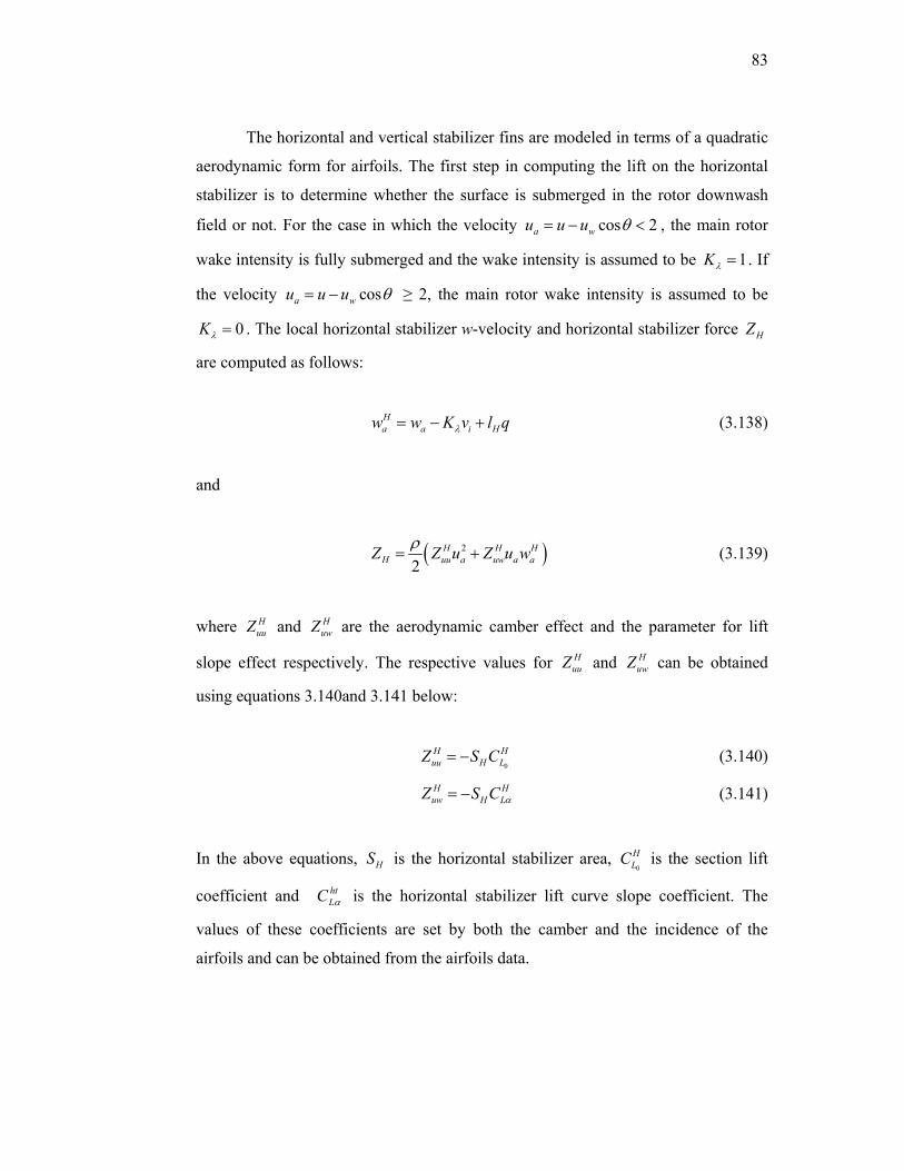
83
The horizontal and vertical stabilizer fins are modeled in terms of a quadratic
aerodynamic form for airfoils. The first step in computing the lift on the horizontal
stabilizer is to determine whether the surface is submerged in the rotor downwash
field or not. For the case in which the velocity cos 2a wu u u θ= − < , the main rotor
wake intensity is fully submerged and the wake intensity is assumed to be 1Kλ = . If
the velocity cosa wu u u θ= − ≥ 2, the main rotor wake intensity is assumed to be
0Kλ = . The local horizontal stabilizer w-velocity and horizontal stabilizer force HZ
are computed as follows:
Ha a i Hw w K v l qλ= − + (3.138)
and
( )2
2H H H
H uu a uw a aZ Z u Z u wρ= + (3.139)
where HuuZ and H
uwZ are the aerodynamic camber effect and the parameter for lift
slope effect respectively. The respective values for HuuZ and H
uwZ can be obtained
using equations 3.140and 3.141 below:
0
H Huu H LZ S C= − (3.140)
H Huw H LZ S C α= − (3.141)
In the above equations, HS is the horizontal stabilizer area, 0
HLC is the section lift
coefficient and htLC α is the horizontal stabilizer lift curve slope coefficient. The
values of these coefficients are set by both the camber and the incidence of the
airfoils and can be obtained from the airfoils data.
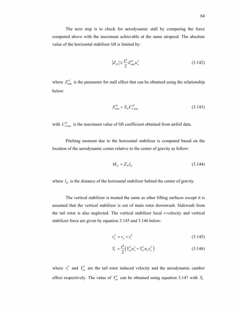
84
The next step is to check for aerodynamic stall by comparing the force
computed above with the maximum achievable at the same airspeed. The absolute
value of the horizontal stabilizer lift is limited by:
2min2H
H aZ Z uρ≤ (3.142)
where minHZ is the parameter for stall effect that can be obtained using the relationship
below:
min maxH H
H LZ S C= (3.143)
with maxHLC is the maximum value of lift coefficient obtained from airfoil data.
Pitching moment due to the horizontal stabilizer is computed based on the
location of the aerodynamic center relative to the center of gravity as follow:
H H HM Z l= (3.144)
where Hl is the distance of the horizontal stabilizer behind the center of gravity.
The vertical stabilizer is treated the same as other lifting surfaces except it is
assumed that the vertical stabilizer is out of main rotor downwash. Sidewash from
the tail rotor is also neglected. The vertical stabilizer local v-velocity and vertical
stabilizer force are given by equation 3.145 and 3.146 below:
V Ta a iv v v= + (3.145)
( )2
2V V V
V uu a uv a aY Y u Y u vρ= + (3.146)
where Tiv and V
uuY are the tail rotor induced velocity and the aerodynamic camber
effect respectively. The value of VuuY can be obtained using equation 3.147 with VS
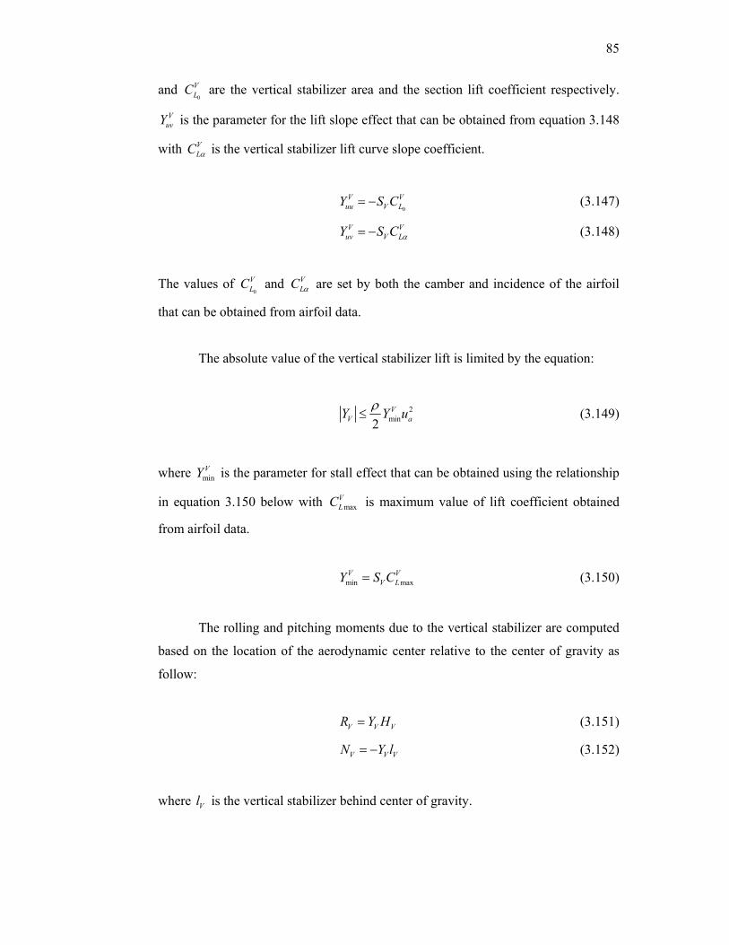
85
and 0
VLC are the vertical stabilizer area and the section lift coefficient respectively.
VuvY is the parameter for the lift slope effect that can be obtained from equation 3.148
with VLC α is the vertical stabilizer lift curve slope coefficient.
0
V Vuu V LY S C= − (3.147)
V Vuv V LY S C α= − (3.148)
The values of 0
VLC and V
LC α are set by both the camber and incidence of the airfoil
that can be obtained from airfoil data.
The absolute value of the vertical stabilizer lift is limited by the equation:
2min2V
V aY Y uρ≤ (3.149)
where minVY is the parameter for stall effect that can be obtained using the relationship
in equation 3.150 below with maxVLC is maximum value of lift coefficient obtained
from airfoil data.
min maxV V
V LY S C= (3.150)
The rolling and pitching moments due to the vertical stabilizer are computed
based on the location of the aerodynamic center relative to the center of gravity as
follow:
V V VR Y H= (3.151)
V V VN Y l= − (3.152)
where Vl is the vertical stabilizer behind center of gravity.

86
3.9 Eigenvalues and Dynamic Mode.
The linearized matrices for hover condition excluding the control rotor (Six
DOF model) are given in Tables 3.4 and 3.5 with the longitudinal and lateral
derivatives being listed in the same matrix form as in Appendix A. Each column and
row is marked with the states and inputs that are being referred to.
Table 3.4 Analytically obtained F matrix in hover with no control rotor
u w q θ v p φ r u -0.0070825 0 0.1261 -9.81 -0.00093895 -0.0292 0 0 w 0 -0.8159 0 0 0 0 0 -0.12 q 0.0377 -0.2775 -0.6718 0 -0.28599 0.1558 0 0.265 θ 0 0 1 0 0 0 0 0 v 0.00093895 0 0.0144 0 -0.06808 0.122823 9.81 0.055 p 0.0094513 0 -0.2942 0 -0.1377 -1.286 0 0.19 φ 0 0 0 0 0 1 0 0 r 0 -1.5246 0 0 1.528 0.122 0 -5.1868
Table 3.5 Analytically obtained G matrix in hover with no control rotor
colδ lonδ latδ pedδ u 5.2981 1.5591 -0.1816 0 w -128.777 0 0 0 q -72.0367 -8.3082 0.9678 9.07 θ 0 0 0 0 v -31.9088 0.0605 -0.5196 5.055 p -321.1883 1.8281 -15.6933 17.322 φ 0 0 0 0 r 178.2831 0 0 17.322
In order to investigate the helicopter dynamics without the control rotor, the
eigenvalues for six DOF model are computed and listed in Table 3.6. Figure 3.23
illustrates the pole position of the hover modes in the complex plane for the coupled
longitudinal and lateral motions. The characteristic equation has four solutions
representing the open loop poles of the longitudinal dynamics. One is a stable
complete pair roots on the real axis and a mildly unstable complex pair. This
instability is a result of the coupling between pitch moment due to longitudinal
velocity and the longitudinal component of the gravitational force due to pitch
(Munzinger, 1998). The stable root is mainly due to the main rotor pitch damping. It

87
has been found that the frequency of the roots is small compared to the rotor speed,
justifying the assumption of only important low frequency response. Since the period
and time to double the amplitude of longitudinal dynamics are large (refer to pitch
oscillation requirement in US Army Aviation Systems Command (1989)), the motion
in hover is still controllable by the pilot. Several feedback loops can be introduced to
improve stability characteristics in hover. One possibility is a lagged feedback of the
pitch rate, introducing damping to the system. This kind of feedback can be provided
by a mechanical feedback system or stabilizer bar used in RC helicopter model.
The lateral dynamics contain lateral velocity, roll angle, lateral cyclic control
and lateral wind velocity. The basic physical systems of lateral and longitudinal
motions are similar, except that the roll moment of inertia is much smaller than the
pitch moment of inertia. This increases the magnitude of roll stability derivatives
relative to pitch derivatives. Poles can be found as one real stable pole due to roll
damping and a stable complex conjugate pole pair due to the rotor flapping effect
and speed stability. Damping moments in roll and pitch are similar in hover.
However, the roll inertia is smaller than the pitch inertia, and the lateral mode has
therefore a higher frequency than the longitudinal mode. The smaller roll inertia
results in a shorter period and less damping of lateral modes that makes it more
difficult for the pilot to control the lateral motion in hover. As for the longitudinal
dynamics, the rate and attitude feedback would be required to stabilize the system. A
control rotor can again provide the mechanical rate feedback of the roll rate and also
improve the stability characteristics.
Table 3.6 Eigenvalues and modes for six DOF model in hovering flight condition
6 DOF Model (8 States)
Mode Eigenvalues Damping Frequency (rad/s)
Longitudinal Oscillation 0.169 ± 0.392 -0.395 0.427
Lateral Oscillation -0.0279 ± 0.765 0.0365 0.765
Heave -0.68 ± 0.142 0.979 0.695
Roll Subsidence -1.68 1 1.68
Yaw -5.28 1 5.28

88
Pole-Zero Map
Real Axis
Imag
inar
y Ax
is
-6 -5 -4 -3 -2 -1 0 1-0.8
-0.6
-0.4
-0.2
0
0.2
0.4
0.6
0.80.60.840.930.9640.9820.991
0.997
0.999
0.60.840.930.9640.9820.991
0.997
0.999
12345
Figure 3.23 Poles of coupled longitudinal and lateral motion for six DOF model with no control rotor
The linearized matrices for hover condition excluding the control rotor (8
DOF model) are given in Tables 3.7 and 3.8 with the longitudinal and lateral
derivatives being listed in the same matrix form as in Appendix A. The same analysis
of eigenvalues leads to the results in Table 3.9 and Figure 3.24.

89
Table 3.7 Analytically obtained F matrix in hover with control rotor
u w q θ v p φ r ,c CRβ ,s CRβ u -0.0070825 0 0.1261 -9.81 -0.00093895 -0.0292 0 0 4.6777 -0.5449 w 0 -0.8159 0 0 0 0 0 -0.12 0 0 q 0.0377 -0.2775 -0.6718 0 -0.28599 0.1558 0 0.265 -24.9271 2.9034 θ 0 0 1 0 0 0 0 0 0 0 v 0.00093895 0 0.0144 0 -0.06808 0.122823 9.81 0.055 0.5449 -4.6777 p 0.0094513 0 -0.2942 0 -0.1377 -1.286 0 0.19 5.4848 -47.0845 φ 0 0 0 0 0 1 0 0 0 0 r 0 -1.5246 0 0 1.528 0.122 0 -5.1868 0 0
,c CRβ 0 0 -0.0421 0 0 1 0 0 -6.834 0
,s CRβ 0 0 -1 0 0 -0.0421 0 0 0 -6.834
Table 3.8 Analytically obtained G matrix in hover with no control rotor
colδ lonδ latδ pedδ u 5.2981 1.5591 -0.1816 0 w -128.777 0 0 0 q -72.0367 -8.3082 0.9678 9.07 θ 0 0 0 0 v -31.9088 0.0605 -0.5196 5.055 p -321.1883 1.8281 -15.6933 17.322 φ 0 0 0 0 r 178.2831 0 0 17.322
,c CRβ 0 -7.8106 0 0
,s CRβ 0 0 7.8106 0
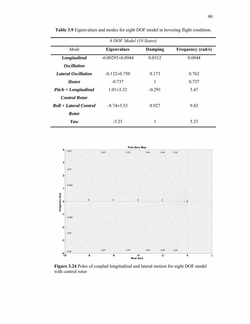
90
Table 3.9 Eigenvalues and modes for eight DOF model in hovering flight condition.
Pole-Zero Map
Real Axis
Imag
inar
y A
xis
-10 -8 -6 -4 -2 0 2-4
-3
-2
-1
0
1
2
3
40.240.460.640.780.870.93
0.97
0.992
0.240.460.640.780.870.93
0.97
0.992
2468
Figure 3.24 Poles of coupled longitudinal and lateral motion for eight DOF model with control rotor
8 DOF Model (10 States)
Mode Eigenvalues Damping Frequency (rad/s)
Longitudinal
Oscillation
-0.00295±0.0944 0.0312 0.0944
Lateral Oscillation -0.132±0.750 0.173 0.762
Heave -0.737 1 0.737
Pitch + Longitudinal
Control Rotor
1.01±3.32 -0.291 3.47
Roll + Lateral Control
Rotor
-8.74±3.53 0.927 9.43
Yaw -5.23 1 5.23

91
Two new complex pole pairs are found in the eight DOF model and it can be
seen that the stability of both oscillation modes is improved and the longitudinal
oscillatory becomes stable. A stable real pole representing helicopter heave mode
indicates that the heave dynamic has an exponentially damped decaying motion. By
introducing two additional control rotor states, the heave dynamic becomes less
oscillate. From the eigenvalues analysis, it is also observed that only small changes
occurred in yaw mode as compared to that of the six DOF model.
For illustrations, the frequency responses from both models were presented in
Figure 3.25(a) and Figure 3.25(b) according to the respective control input and
compared to the model using flight data. As shown in Figure 3.25(a) and Figure
3.25(b), the six DOF dynamic model with eight states accurately predicts the low
frequency rate response. The model does not capture the coupled rotor-fuselage
mode and leads to mismatches in both the magnitude and phase regions. It is
necessary to include in the analysis of helicopter dynamic, the dynamical coupling
between the main rotor and helicopter fuselage. To include the rotor-fuselage
coupling effects, the rotor dynamic equation (flapping dynamic) need to be
accounted for and coupled in the fuselage equation of motions. It has been shown in
Figure 3.25(a) and Figure 3.25(b) that the modeling of flapping equations and
stabilizer bar dynamic produce more accurate results. Discarding these coupling
effect leads to the limitation of helicopter model accuracy in medium to high
frequency (Mettler et al., 2000a).
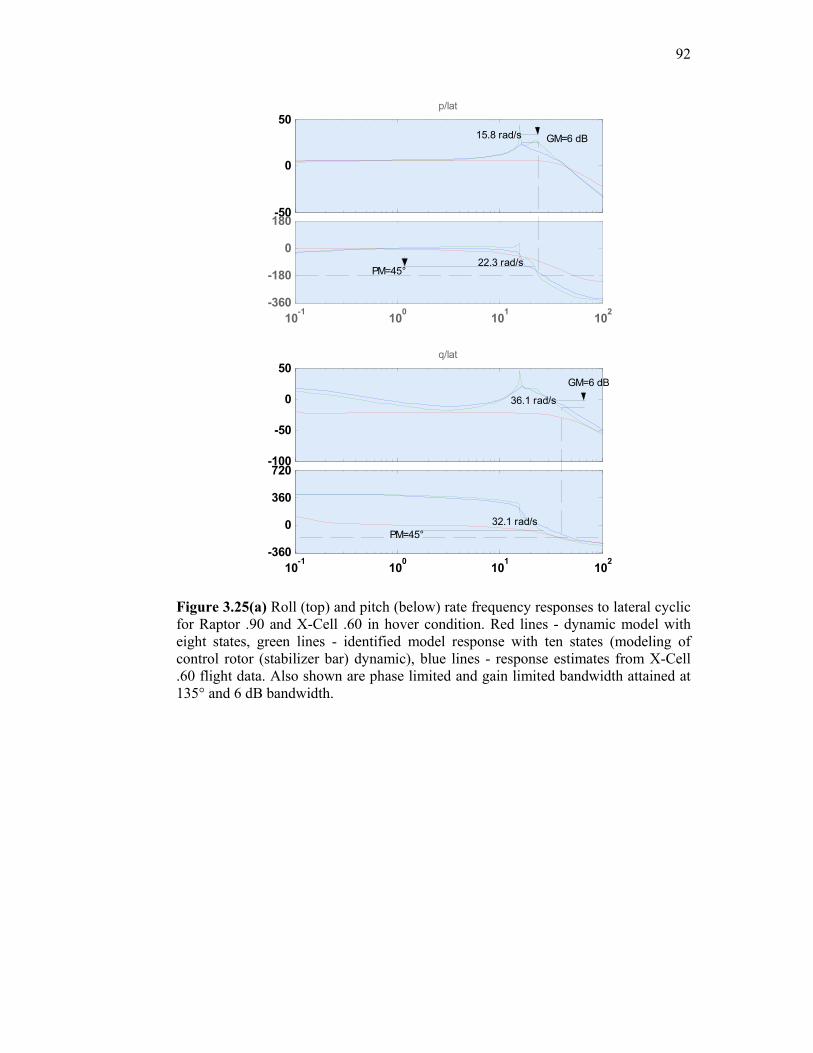
92
-50
0
50p/lat
10-1 100 101 102-360
-180
0
180
-100
-50
0
50q/lat
10-1 100 101 102-360
0
360
720
15.8 rad/s GM=6 dB
PM=45° 22.3 rad/s
GM=6 dB
PM=45°
36.1 rad/s
32.1 rad/s
Figure 3.25(a) Roll (top) and pitch (below) rate frequency responses to lateral cyclic for Raptor .90 and X-Cell .60 in hover condition. Red lines - dynamic model with eight states, green lines - identified model response with ten states (modeling of control rotor (stabilizer bar) dynamic), blue lines - response estimates from X-Cell .60 flight data. Also shown are phase limited and gain limited bandwidth attained at 135° and 6 dB bandwidth.

93
-100
0
100p/lon
10-1 100 101 102-180
0180360540
-50
0
50
100q/lon
10-1 100 101 102-360
-180
0
180
GM=6 dB
GM=6 dB
PM=45°
PM=45°
23.8 rad/s
16.7 rad/s
15.5 rad/s
15.64 rad/s
Figure 3.25(b) Roll (top) and pitch (below) rate frequency responses to longitudinal cyclic for Raptor .90 and X-Cell .60 in hover condition. Red lines - dynamic model with 8 states, green lines - identified model response with 10 states (modeling of control rotor (stabilizer bar) dynamic), blue lines - response estimates from X-Cell .60 flight data. Also shown are phase limited and gain limited bandwidth attained at 135° and 6 dB bandwidth.
3.10 Conclusion
This chapter described the mathematical model used for the stability and
control simulation. The important helicopter parameters such physical dimensions,
moment inertia, rotor flapping moment, aerodynamic input and control rigging curve
were determined either from physical measurement, look-up table or experimental
test. The helicopter nonlinear mathematical model can be established using these

94
parameters. The nonlinear helicopter mathematical model was then linearized using
small perturbation theory for stability analysis and linear feedback control system
design. The linear feedback control system design will be discuss in detail later in
Chapter 4. The generation of forces and moments from each source such as
helicopter main rotor, tail rotor, control rotor and other lifting surfaces has also been
discussed in detail in this chapter. Two linearized mathematical model have been
obtained from the analysis and it has been shown that it is essential to include the
modeling of rotor flapping equations and stabilizer bar dynamic produce more
accurate frequency response result compare to six DOF dynamic model. As
suggested in stability analysis for hover model, several feedback loops can be
introduced to improve the stability characteristic of helicopter model in hover
condition.
CHAPTER 4
CONTROL SYSTEM ANALYSIS
4.1 Introduction
In this part of the research, it is aimed at the construction of a controller that
will able to read the real time referance trajectory and issues the
feedforward/feedback control output for the helicopter airframe in real time
situations. In Figure 4.1, the hierarchical structure that has been developed for the
UAV model application is presented. The main target in this research is to develop
the lower two layers, i.e. the waypoint generator and the regulation layers. The
waypoint generator receives the motion command from the strategic planner (human
operator) and activates the proper control sets and sends the referance trajectory data
in real time. The waypoint generator consists of a single PIC microcontroller unit on
ground station which was programmed to send flight mode commands such as hover,
take-off, landing, move forward and turning to on-board computer to perform
automatic feedforward/feedback control output for helicopter airframe.
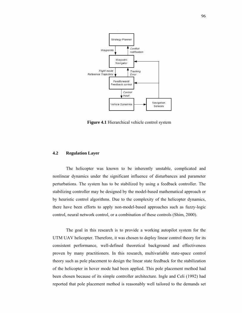
96
Figure 4.1 Hierarchical vehicle control system
4.2 Regulation Layer
The helicopter was known to be inherently unstable, complicated and
nonlinear dynamics under the significant influence of disturbances and parameter
perturbations. The system has to be stabilized by using a feedback controller. The
stabilizing controller may be designed by the model-based mathematical approach or
by heuristic control algorithms. Due to the complexity of the helicopter dynamics,
there have been efforts to apply non-model-based approaches such as fuzzy-logic
control, neural network control, or a combination of these controls (Shim, 2000).
The goal in this research is to provide a working autopilot system for the
UTM UAV helicopter. Therefore, it was chosen to deploy linear control theory for its
consistent performance, well-defined theoretical background and effectiveness
proven by many practitioners. In this research, multivariable state-space control
theory such as pole placement to design the linear state feedback for the stabilization
of the helicopter in hover mode had been applied. This pole placement method had
been chosen because of its simple controller architecture. Ingle and Celi (1992) had
reported that pole placement method is reasonably well tailored to the demands set

97
by the design criteria required by ADS-33C. Furthermore the controller proposed
satisfied the design criteria even when rotor, inflow and other higher order dynamics
were included. In the following sub-section, the formal statement of the stabilizing
feedback controller design is presented:
Problem Statement:
Suppose the kinematics is given as follows: TPTP VX =
bTPB
TP VRX →=
b
dtd ω
θφθφφφθφθφ
ψθφ
⎥⎥⎥
⎦
⎤
⎢⎢⎢
⎣
⎡−=
⎥⎥⎥
⎦
⎤
⎢⎢⎢
⎣
⎡
coscoscossin0sincos0
tancostansin1 (4.1)
and the linear dynamics as,
BuAxx += (4.2)
Cxy = (4.3)
where
[ ]TTP zyxX =
[ ]TTPz
TPy
TPx
TP vvvV =
[ ]Tb wvuV =
[ ]Tb rqpw =
[ ]Tss rwbaqpvux 11θφ=
[ ]Trba refMssuuuuu θ11
=
and
[ ]TTPz
TPy
TPx rqpwvuvvvzyxy ψθφ=
The TPBR → expression represents the rotational transformation matrix from body
coordinate system to tangent plane system and bω is the angular velocity in body

98
coordinate system. It is needed to achieve a control law that stabilizes the vehicle
dynamics and steer the vehicle to follow the desired trajectory, i.e.
( ) ( ) ( ) ( ) ( )( )ttztytxty refTPref
TPref
TPrefref ψ,,,= (4.4)
As partial requirement, it is also needed to find a static or dynamic stabilizing
feedback control law:
( ) ( )( )tyftu fb = (4.5)
4.3 State Space Controller Design
A typical feedback control system in Figure 4.2 can be represented in state
space system as Equations 4.2 and 4.3 where the light lines are scalars and the heavy
lines are vectors.
Figure 4.2 A State Space representation of a plant (Nise, 2000)
In this typical feedback control system, the output, y , is fed back to the summing
junction. In linear state feedback design, each state variable is fed back to the
control,u , through a gain, ik to yield the required closed-loop pole values. The
feedback through the gains, ik is represented in Figure 4.3 by the feedback vector –
K.
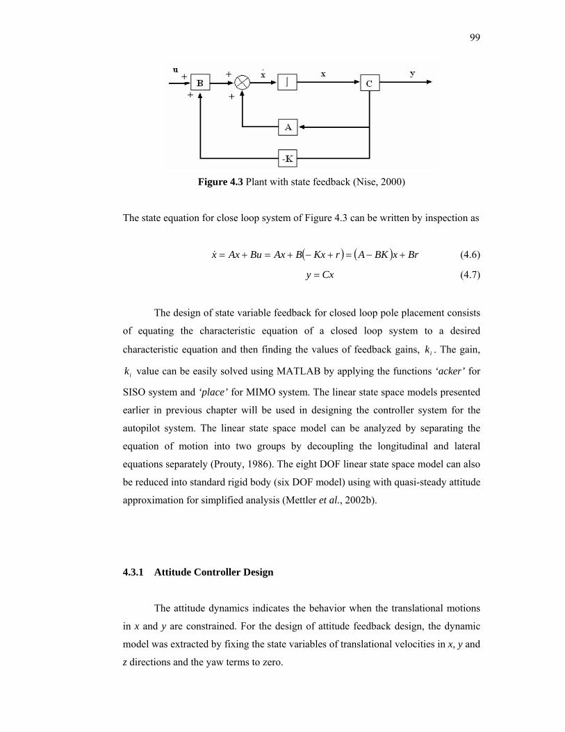
99
Figure 4.3 Plant with state feedback (Nise, 2000)
The state equation for close loop system of Figure 4.3 can be written by inspection as
( ) ( ) BrxBKArKxBAxBuAxx +−=+−+=+= (4.6)
Cxy = (4.7)
The design of state variable feedback for closed loop pole placement consists
of equating the characteristic equation of a closed loop system to a desired
characteristic equation and then finding the values of feedback gains, ik . The gain,
ik value can be easily solved using MATLAB by applying the functions ‘acker’ for
SISO system and ‘place’ for MIMO system. The linear state space models presented
earlier in previous chapter will be used in designing the controller system for the
autopilot system. The linear state space model can be analyzed by separating the
equation of motion into two groups by decoupling the longitudinal and lateral
equations separately (Prouty, 1986). The eight DOF linear state space model can also
be reduced into standard rigid body (six DOF model) using with quasi-steady attitude
approximation for simplified analysis (Mettler et al., 2002b).
4.3.1 Attitude Controller Design
The attitude dynamics indicates the behavior when the translational motions
in x and y are constrained. For the design of attitude feedback design, the dynamic
model was extracted by fixing the state variables of translational velocities in x, y and
z directions and the yaw terms to zero.

100
The design specification for the controller design is selected according to
Aeronautical Design Standard for military helicopter (ADS-33C). In Figure 4.4, the
damping ratio limits on pitch (roll) oscillations in hover and low speed are specified
to be greater than 0.35 (OS% ≤ 30.9) and the settling time to be achieved in less than
10 seconds. Therefore for the purpose of the attitude controller design, the
percentage of overshoot (OS) is set to be 10% and the settling time of 5 seconds
should be achieved with no steady state error.
Figure 4.4 Limits on pitch (roll) oscillations – hover and low speed according to Aeronautical Design Standard for military helicopter (ADS-33C) (US Army Aviation Systems Command, 1989)
Using the ‘place’ and ‘ltiview’ functions in MATLAB, the performance of
attitude controller can be achieved according to design requirement for both the pitch
and roll axes. In the pitch axis response, the poles are placed at p = -0.8 + 1.095i, -0.8
– 1.095i and -0.00842 in order to achieve 10% OS and 5 second settling time. The
phase variable feedback gain is found to be [ ]0.009 0.0455 0.0417Kθ = − . The
resulting control law for pitch dynamic is given

101
by 1 0.0009 0.0455 0.0417B u q θ= − + . In the roll axis response, the poles are placed
at p = -0.8 + 1.095i, -0.8 – 1.095i and -0.0622 in order to achieve 10% OS and 5
second settling time. The corresponding phase variable feedback is found to
be [ ]0.0103 0.3872 0.0673Kφ = − − . The resulting control law for roll dynamic is
given by φ0673.03872.00103.01 −−= pvA . The time response and Bode diagram
plots for both axes are shown in Figures 4.5(a) and 4.5(b). In Figure 4.6, both
controller bandwidth and time delay have been shown to meet the Level 1
requirements specify in Section 3.3.21 of the Military Handling Qualities
Specification ADS-33C.
Bode Diagram
Frequency (rad/sec)
Linear Simulation Results
Time (sec)
Ampl
itude
10-3
10-2
10-1
100
101
102
-180
-135
-90
-45
0
Phas
e (d
eg)
-80
-60
-40
-20
0
20
Mag
nitu
de (d
B)
0 1 2 3 4 5 6 7 8 9 100
1
2
3
4
5
6
7
8x 10
-3
Pitc
h An
gle
(rad
)
Figure 4.5(a) Attitude compensator design for pitch axis response due to 0.007 rad longitudinal cyclic step command. The phase variable feedback gain is found to be [ ]0.009 0.0455 0.0417Kθ = − . The bandwidth,
θωBW is located at 2.39 rad/s
and the phase delay, θ
τ P = 0
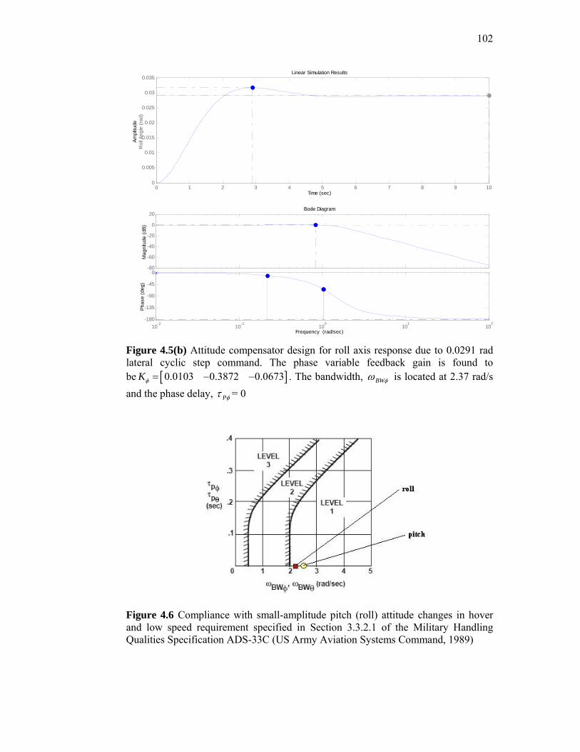
102
Bode Diagram
Frequency (rad/sec)
Linear Simulation Results
Time (sec)
Ampl
itude
10-2
10-1
100
101
102
-180
-135
-90
-45
0
Phas
e (d
eg)
-80
-60
-40
-20
0
20
Mag
nitu
de (d
B)
0 1 2 3 4 5 6 7 8 9 100
0.005
0.01
0.015
0.02
0.025
0.03
0.035
Rol
l Ang
le (r
ad)
Figure 4.5(b) Attitude compensator design for roll axis response due to 0.0291 rad lateral cyclic step command. The phase variable feedback gain is found to be [ ]0.0103 0.3872 0.0673Kφ = − − . The bandwidth, φωBW is located at 2.37 rad/s and the phase delay, φτ P = 0
Figure 4.6 Compliance with small-amplitude pitch (roll) attitude changes in hover and low speed requirement specified in Section 3.3.2.1 of the Military Handling Qualities Specification ADS-33C (US Army Aviation Systems Command, 1989)

103
4.3.2 Velocity Control
Once the attitude dynamics are stabilized, the feedback gain for the velocity
dynamic has to be found using similar approach. For velocity control, the design of
the phase variable feedback gains should yield 10% overshoot and a settling time of
5 seconds. In longitudinal velocity mode, the poles were selected to be placed at p = -
0.8 + 1.095i, -0.8 – 1.095i and -57.7 in order to achieve 10% OS and 5 second
settling time. The suitable feedback gains were found to be
[ ]0.2428 1.2783 2.1660uK = − for longitudinal velocity. The resulting control law
for longitudinal velocity dynamic is given by 1 0.2428 1.2783 2.166B u q θ= − + + . In
lateral velocity mode, the poles were selected to be placed at p = -0.8 + 1.095i, -0.8 –
1.095i and -5 in order to achieve 10% OS and 5 second settling time. The
corresponding suitable feedback gains were found to be
[ ]0.028 0.5682 0.3481vK = − − − for lateral velocity. The resulting control law for
lateral velocity dynamic is given by φ3481.05682.0028.01 −−−= pvA . Figures
4.7(a) and 4.7(b) show the step response of the velocity dynamic in longitudinal and
lateral modes.
Step Response
Time (sec)
Ampl
itude
0 2 4 6 8 10 120
0.2
0.4
0.6
0.8
1
1.2
1.4
horiz
onta
l vel
ocity
, u (m
/s)
Figure 4.7(a) Velocity compensator design for longitudinal velocity mode due to longitudinal cyclic step command

104
Step Response
Time (sec)
Ampl
itude
0 1 2 3 4 5 60
0.2
0.4
0.6
0.8
1
1.2
1.4
Late
ral V
eloc
ity, v
(m/s
)
Figure 4.7(b) Velocity compensator design for lateral velocity mode due to lateral cyclic step command
4.3.3 Heave and Yaw Control
The helicopter heave or vertical rate dynamic response can be represented as a first
order system transfer function according to Aeronautical Design Standard for
military helicopter (ADS-33C) (US Army Aviation Systems Command, 1989). The
first order transfer function for vertical rate dynamic response is given by equation
4.8. ADS-33C has listed a procedure for obtaining the equivalent time domain
parameters for the vertical rate dynamic response to collective controller in Figure
4.8. For Level 1 handling quality, as defined in Cooper-Harper Handling Qualities
Rating (HQR) Scale, the vertical rate response shall have a qualitative first order
appearance for at least 5 second following a step collective input (See Table 4.1).
Pitch, roll, and heading excursions shall be maintained essentially constant. In order
to achieve this, the gains are chosen to be wK = -2.14 and the resulting control law
for heave dynamic is given by 0 2.14wθ = − . The step response for the heave
controller in shown in Figure 4.9.
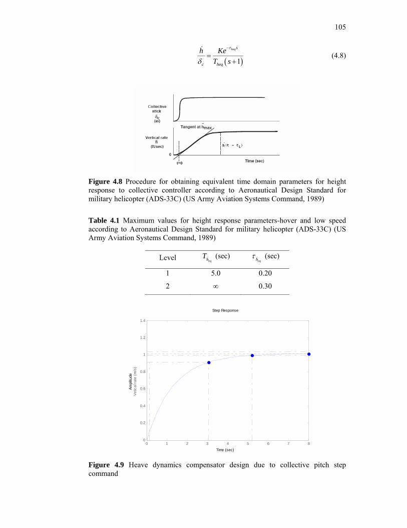
105
( )1
heqs
c heq
h KeT s
τ
δ
−
=+
(4.8)
Figure 4.8 Procedure for obtaining equivalent time domain parameters for height response to collective controller according to Aeronautical Design Standard for military helicopter (ADS-33C) (US Army Aviation Systems Command, 1989)
Table 4.1 Maximum values for height response parameters-hover and low speed according to Aeronautical Design Standard for military helicopter (ADS-33C) (US Army Aviation Systems Command, 1989)
Level eqhT (sec) eqhτ (sec)
1 5.0 0.20
2 ∞ 0.30
Step Response
Time (sec)
Ampl
itude
0 1 2 3 4 5 6 7 80
0.2
0.4
0.6
0.8
1
1.2
1.4
Vetic
al ra
te (m
/s)
Figure 4.9 Heave dynamics compensator design due to collective pitch step command
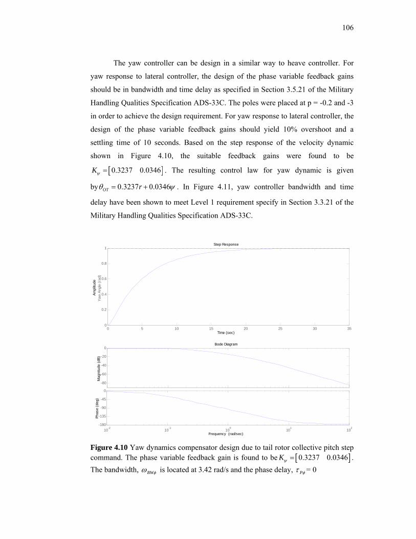
106
The yaw controller can be design in a similar way to heave controller. For
yaw response to lateral controller, the design of the phase variable feedback gains
should be in bandwidth and time delay as specified in Section 3.5.21 of the Military
Handling Qualities Specification ADS-33C. The poles were placed at p = -0.2 and -3
in order to achieve the design requirement. For yaw response to lateral controller, the
design of the phase variable feedback gains should yield 10% overshoot and a
settling time of 10 seconds. Based on the step response of the velocity dynamic
shown in Figure 4.10, the suitable feedback gains were found to be
[ ]0.3237 0.0346Kψ = . The resulting control law for yaw dynamic is given
by 0.3237 0.0346OT rθ ψ= + . In Figure 4.11, yaw controller bandwidth and time
delay have been shown to meet Level 1 requirement specify in Section 3.3.21 of the
Military Handling Qualities Specification ADS-33C.
Bode Diagram
Frequency (rad/sec)
Step Response
Time (sec)
Ampl
itude
10-2
10-1
100
101
102
-180
-135
-90
-45
0
Phas
e (d
eg)
-80
-60
-40
-20
0
Mag
nitu
de (d
B)
0 5 10 15 20 25 30 350
0.2
0.4
0.6
0.8
1
Yaw
Ang
le (r
ad)
Figure 4.10 Yaw dynamics compensator design due to tail rotor collective pitch step command. The phase variable feedback gain is found to be [ ]0.3237 0.0346Kψ = . The bandwidth, φωBW is located at 3.42 rad/s and the phase delay, φτ P = 0

107
Figure 4.11 Compliance with small-amplitude heading changes in hover and low speed requirement specified in Section 3.3.5.1 of the Military Handling Qualities Specification ADS-33C (US Army Aviation Systems Command, 1989)
4.3.4 Position Control
For position control, the design of the phase variable feedback gains should
yield 10% overshoot and a settling time of 5 seconds. In longitudinal position mode,
the poles were selected to be placed at p = -0.8 + 1.095i, -0.8 – 1.095i, -0.5 and -4. In
order to achieve 10% OS and 5 second settling time, the suitable feedback gains were
found to be [ ]0.0449 0.1358 0.6271 1.3017xK = − − for longitudinal velocity.
The resulting control law for longitudinal velocity dynamic is given by
1 0.0449 0.1358 0.6271 1.3017B x u q θ= + − − . In lateral position mode, the poles were
selected to be placed at p = -0.8 + 1.095i, -0.8 – 1.095i, -2 and -3. In order to achieve
10% OS and 5 second settling time, the suitable feedback gains were found to be
[ ]0.0714 0.1056 0.3308 0.9613yK = − − − − for lateral velocity. The resulting
control law for lateral position dynamic is given by
1 0.0714 0.1056 0.3308 0.9613A y v p θ= − − − − . The time response plots for both axes
(longitudinal and lateral) are shown in Figures 4.12(a) and 4.12(b) respectively.
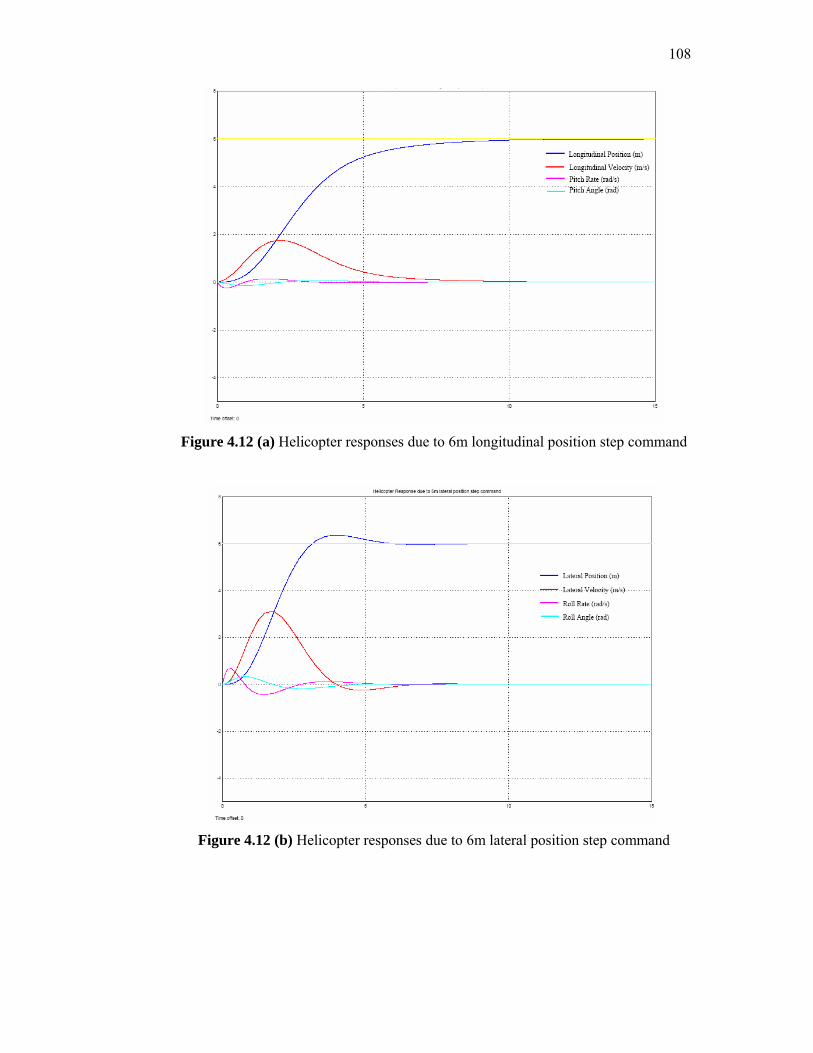
108
Figure 4.12 (a) Helicopter responses due to 6m longitudinal position step command
Figure 4.12 (b) Helicopter responses due to 6m lateral position step command
109
4.4 Conclusion
This chapter has shown results of using state feedback method in designing
attitude, velocity, heave and yaw controller for UTM autonomous helicopter model.
The linear eight DOF state space model can be reduced to rigid body form with
quasi-steady attitude approximation and can be decoupled to allow an analysis of
lateral/longitudinal dynamics separately from yaw/heave dynamics in hover
condition. The phase variable feedback gains were calculated for each helicopter
dynamics in hover condition to satisfy the requirements contained in the ADS-33C.
CHAPTER 7
CONCLUSION
7.1 Concluding Remarks
The main focus of this project is to develop the autopilot system. In order to
achieve the objective, a mathematical model used for the stability and control
simulation had been derived The important helicopter parameters such physical
dimensions, moment inertia, rotor flapping moment, aerodynamic input and control
rigging curve were determined either from physical measurement, look-up table or
experimental test. The helicopter nonlinear mathematical model can be established
using these parameters. The nonlinear helicopter mathematical model was then
linearized using small perturbation theory for stability analysis and linear feedback
control system design. The generation of forces and moments from each source such
as helicopter main rotor, tail rotor, control rotor and other lifting surfaces has also
been analyzed in this project. The influence rotor flapping and stabilizer bar dynamic
modeling have produce more accurate frequency response result compare to six DOF
dynamic model. As suggested in stability analysis for hover model, several feedback
loops can be introduced to improve the stability characteristic of helicopter model in
hover condition.
The linear eight DOF state space model in hovering condition can be reduced
to rigid body form with quasi-steady attitude approximation and can be decoupled to
allow an analysis of lateral/longitudinal dynamics separately from yaw/heave
dynamics in hover condition. The attitude, velocity, heave and yaw controller for the

170
autopilot system has been designed using state feedback method. The phase variable
feedback gains were calculated for each helicopter dynamics in hover condition to
satisfy the performance requirements contained in the ADS-33C.
An autopilot system for UAV helicopter model had been designed using on-
board computing before the controller design can be tested. A conventional
helicopter model had been selected as UAV platform and the hardware and software
used to autonomously pilot the helicopter are described in detail in this thesis. The
complete autopilot system integration with the helicopter had been done after all the
electronics were built and installed considering several factors such as power supply
regulation, avionic box mounting design, electromagnetic and radio interference. In
order to allow for manual override of computer control, a manual to automatic switch
was designed where the pulse width signal decode is done on single Microchip
microcontroller. The application of manual to automatic switch helps human pilot to
regain control of the helicopter if the autopilot fails during flight.
The performance of autopilot system developed had been evaluated through
the tests conducted in test rig, preliminary test and actual flight test. The proposed
hovering controller has shown capable of stabilizing the helicopter attitude angles.
The positional, velocity and heave controller design could not be implemented in the
tests due to limitation of resources in this project. A GPS device should be used as
part of autopilot’s sensor to give position information to flight computer. The
combination of AHRS and GPS device could enable better hovering stabilization
control of helicopter model with position hold capabilities.
Through flight testing, the developed autopilot system had satisfactorily
flown the UAV helicopter model. Hence it is concluded that the proposed autopilot
system was successfully developed for the UAV helicopter model. The list of
author’s publication paper can be viewed in Appendix E.

171
7.2 Recommendations of Future Work
The work in this thesis suggests that future enhancement can be carried out to
further improve the design for achieving better performance or a more complete
operation. Below are some of the proposed future works:
The first recommendation is the improvement of the hardware of autopilot
system. Up to now, the UAV helicopter was able to maintain its attitude angle. From
the flight test it was also observed that the helicopter would sway slowly from its
hover position if there was a crosswind. A GPS system can be incorporated into the
system in order to control the position of the helicopter while stabilizing the attitude
of the aircraft.
The second recommendation is the extensive study on the helicopter vibration
cause by the main rotor, tail rotor and engine. Its effect on the sensors installed on
the autopilot system is very crucial since sensitive electronics such as AHRS and
later camera needed to be protected from harsh vibrations produced by the helicopter.
The final recommendation is the improvement of control algorithm used in
the autopilot system. The control algorithm of autopilot system can be improved by
adding fault detection control scheme where such control algorithm can be used as
protection for helicopter in failure events such as main rotor collective pitch failure,
sensor failure or even structural failure (break in transmission). Taking the example
of failure in collective pitch actuator, a control switch can be designed in the low
level flight controller to reconfigure the control to rpm control. By doing this, the
flight computer can still be able to control the throttle or rotorspeed of the helicopter
and hence provides a mean of safe landing of the helicopter.
CHAPTER 6
SYSTEM EVALUATION
6.1 Introduction
Controlling a remote control helicopter is difficult and careful
experimentation is essential in building a working UAV helicopter prototype. For the
testing of autopilot developed in this research, a six Degree-of-Freedom (6-DOF)
testbed for safe indoor helicopter flight was developed. It was mainly as a safety
device for preventing crashes and out-of-control flight. As shown in Figure 6.1, the
testbed supports an RC helicopter that could fly freely in a pyramid-shaped volume
of base area 2.5m x 2.5m and height of 2m. The helicopter is fastened to support
structure and connected to the testbed stand by four connecting rods that are free to
move through two-degree-of-freedom (2-DOF) joints as illustrated in Figure 6.2. An
important issue of great concern is the effects of the testbed components on the
helicopter dynamics in free flight. To minimize inertial variations, the helicopter
support structure and connecting rod was built from light-weight metal such as
aluminum that could minimize weight and friction. Minimizing friction is essentially
critical since friction has the tendency to significantly dampen helicopter movement.
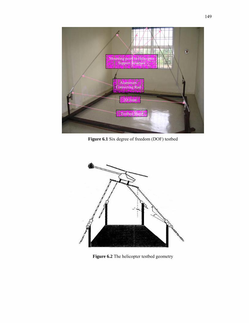
149
Figure 6.1 Six degree of freedom (DOF) testbed
Figure 6.2 The helicopter testbed geometry
Aluminum Connecting Rod
Testbed Stand
2D Joint
Mounting point to Helicopter Support Structure
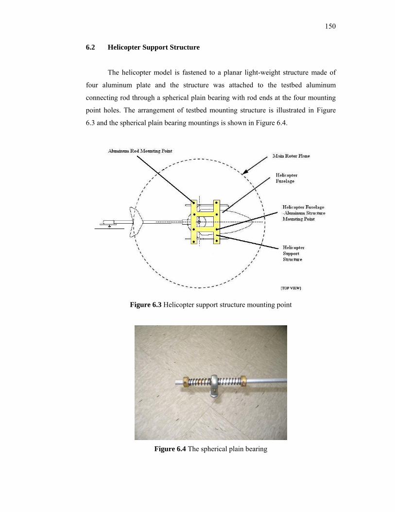
150
6.2 Helicopter Support Structure
The helicopter model is fastened to a planar light-weight structure made of
four aluminum plate and the structure was attached to the testbed aluminum
connecting rod through a spherical plain bearing with rod ends at the four mounting
point holes. The arrangement of testbed mounting structure is illustrated in Figure
6.3 and the spherical plain bearing mountings is shown in Figure 6.4.
Figure 6.3 Helicopter support structure mounting point
Figure 6.4 The spherical plain bearing
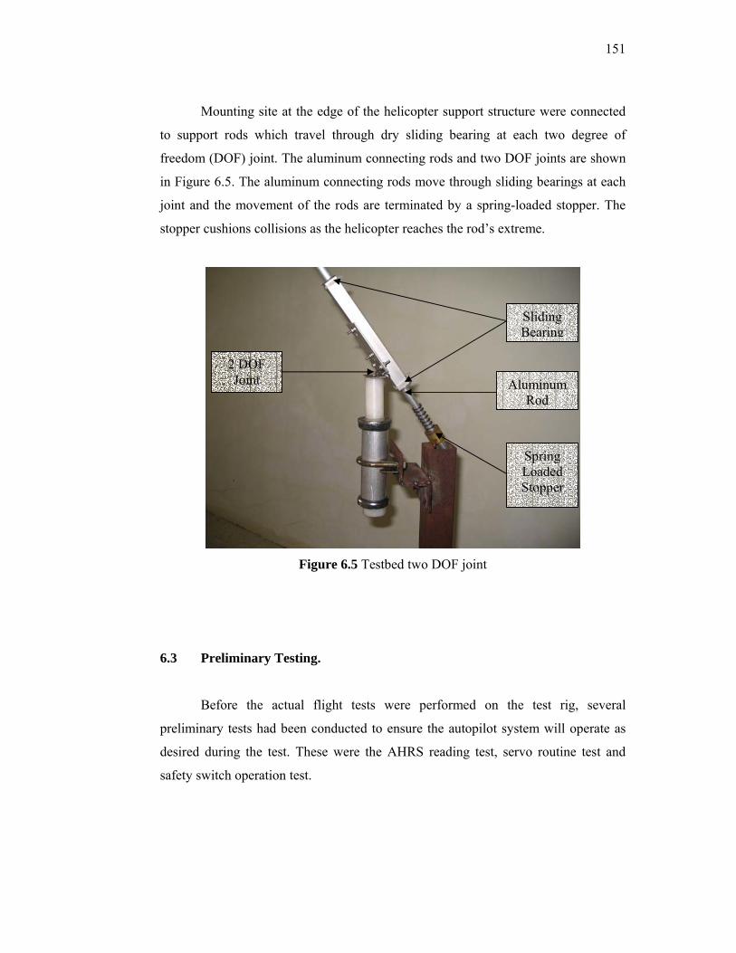
151
Mounting site at the edge of the helicopter support structure were connected
to support rods which travel through dry sliding bearing at each two degree of
freedom (DOF) joint. The aluminum connecting rods and two DOF joints are shown
in Figure 6.5. The aluminum connecting rods move through sliding bearings at each
joint and the movement of the rods are terminated by a spring-loaded stopper. The
stopper cushions collisions as the helicopter reaches the rod’s extreme.
Figure 6.5 Testbed two DOF joint
6.3 Preliminary Testing.
Before the actual flight tests were performed on the test rig, several
preliminary tests had been conducted to ensure the autopilot system will operate as
desired during the test. These were the AHRS reading test, servo routine test and
safety switch operation test.
Aluminum Rod
Spring Loaded Stopper
Sliding Bearing
2 DOF Joint
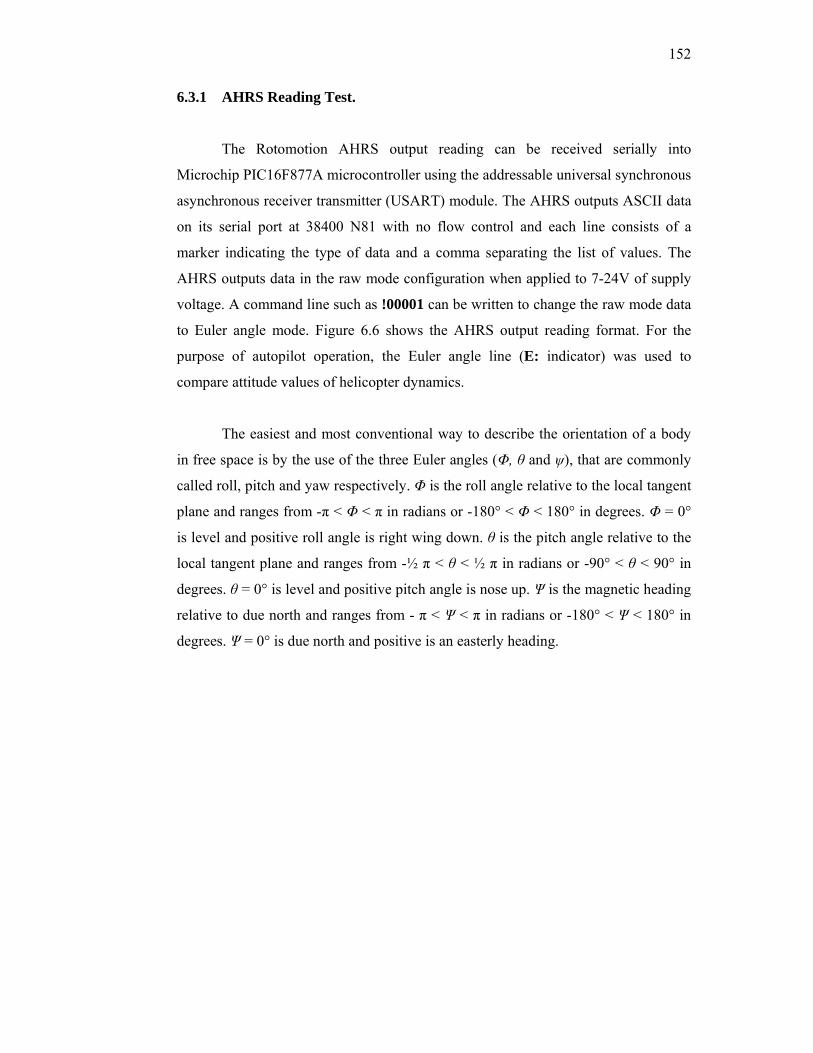
152
6.3.1 AHRS Reading Test.
The Rotomotion AHRS output reading can be received serially into
Microchip PIC16F877A microcontroller using the addressable universal synchronous
asynchronous receiver transmitter (USART) module. The AHRS outputs ASCII data
on its serial port at 38400 N81 with no flow control and each line consists of a
marker indicating the type of data and a comma separating the list of values. The
AHRS outputs data in the raw mode configuration when applied to 7-24V of supply
voltage. A command line such as !00001 can be written to change the raw mode data
to Euler angle mode. Figure 6.6 shows the AHRS output reading format. For the
purpose of autopilot operation, the Euler angle line (E: indicator) was used to
compare attitude values of helicopter dynamics.
The easiest and most conventional way to describe the orientation of a body
in free space is by the use of the three Euler angles (Φ, θ and ψ), that are commonly
called roll, pitch and yaw respectively. Φ is the roll angle relative to the local tangent
plane and ranges from -π < Φ < π in radians or -180° < Φ < 180° in degrees. Φ = 0°
is level and positive roll angle is right wing down. θ is the pitch angle relative to the
local tangent plane and ranges from -½ π < θ < ½ π in radians or -90° < θ < 90° in
degrees. θ = 0° is level and positive pitch angle is nose up. Ψ is the magnetic heading
relative to due north and ranges from - π < Ψ < π in radians or -180° < Ψ < 180° in
degrees. Ψ = 0° is due north and positive is an easterly heading.

153
Figure 6.6 AHRS output data format
Since the PICBasic compiler and Microchip microcontroller only handle
unsigned integers (any non-digit characters receive will be discarded) in its
comparison operation, the string data modifier command should be used to receive
each character and stored in array variables. In order to ensure that the ASCII data
received is interpreted correctly by the microcontroller into true decimal numbers, a
simple test can be conducted using LED or oscilloscope to test the negative sign and
absolute value of Euler angle readings. Since PIC16F877A’s Port B is left unused in
the PCB board, the LED can be connected directly to each pin on Port B as shown in
Figure 6.7. In the programming code, each ASCII character received by
microcontroller will be converted into the decimal value as presented in standard
ASCII character set. Simple IF-THEN rules can be applied to check the negative
sign, decimal values and point sign in the incoming data store in array variables. If
comparison made gives true condition, HIGH command is given to light the LED at
specific location. Figure 6.8 gives the overall view of test carried out.

154
Figure 6.7 LED connections to PIC18F4520 Port B
Figure 6.8 AHRS reading testing on protoboard
AHRS
Microcontroller unit
LED
Servo
Protoboard

155
6.3.2 Servo Routine Testing
Similar test can be conducted to test the servo timing. It is necessary to feed
the pulse signal to servomotor 50 to 60 times a second. It is important to keep this in
mind when running multiple servomotors or other time critical applications. The next
step in the testing is to ensure that the servo motor moves in the correct direction in
order to stabilize the helicopter.
6.3.3 Manual to Automatic Switch Testing
A manual to automatic switch was designed for the autopilot system which
enable human pilot to gain control of the helicopter if autopilot system fails during
flight. Standard hobby radio control equipment is used for this task. To allow for
manual override of computer control, a switch box was designed as had been
discussed in detail in the chapter 5. The pulse width decode was done on a single
Microchip PIC16F84A chip and the connections between the standard RC
equipments are illustrated in Figure 6.9. A preliminary test is carried out to ensure
that the manual to automatic switch function correctly.
Figure 6.9 Manual to automatic switch operation testing
PIC16F877A
PIC1684A
RC Receiver
156
6.4 Flight Test
The flight tests had been conducted in three phases. The first phase was the
full flown flight by human pilot (Manual Flight) to check all of the mechanical
components and RC control system in flight are in operating conditions. The second
phase was the initial flight test which was conducted to test the mechanical
construction aspect of the avionic box. The third phase was the partially computer
controlled flight. During this phase, three of the channels were controlled under
computer guidance while all others manually.
6.4.1 Manual Flight
Actual flight test is the crucial stage to validate the proposed control,
hardware and software integrations. Several inspections before flight need to be
carried out and these procedures can be divided into control system check and flying
adjustment. The standard checklist procedure stated in the Thunder Tiger Raptor 90
assembly and maintenance manual can be used before attempting an actual flight test
(Thunder Tiger Corp, 2004). Conducting a test flight is by nature a very dangerous
operating condition for the helicopter type airframe used in this research.
The manual flight test was conducted to ensure that the helicopter is in proper
tuning and can be controlled with ease by the test pilot. In this test, the test pilot will
conduct routine tests to check the performance of the OS MAX-91SX-HRING C
SPEC PS engine. Power failure is rarely a serious threat to the safety of the fixed-
wing model aircraft since it can usually glide down to a safe landing. On the other
hand for the helicopter, it is vitally important that the engine is kept running and that
there is a quick and reliable response to the throttle in order to ensure safe ascent and
descent of the model. For the OS MAX-91SX-HRING C SPEC PS engine, there are

157
two main adjustable mixture controls for its Type 60M carburetor that need to be
tuned:
i. The High-Speed (Main) Needle Valve
The high speed needle valve is set to produce maximum power at full throttle
by establishing the basic fuel to air mixture strength. This is then maintained
by the carburetor's automatic mixture control system to cover the engine's
requirements at reduced throttle settings.
ii. The Idle Mixture Control Screw
This provides the mean of manually adjusting the 60M's mixture control
valve. By setting the Mixture Control Screw for the best idling performance,
the mixture control valve automatically ensures that fuel is accurately
metered to maintain the correct mixture strength as the throttle is opened.
The complete carburetor adjustment procedure can be referred from OS Engine Mfg.
Co. Ltd. (2003) and the adjustment procedure is summarized in Figure 6.10.

158
Figure 6.10 Carburetor adjustment chart (OS Engine Mfg. Co. Ltd., 2003)
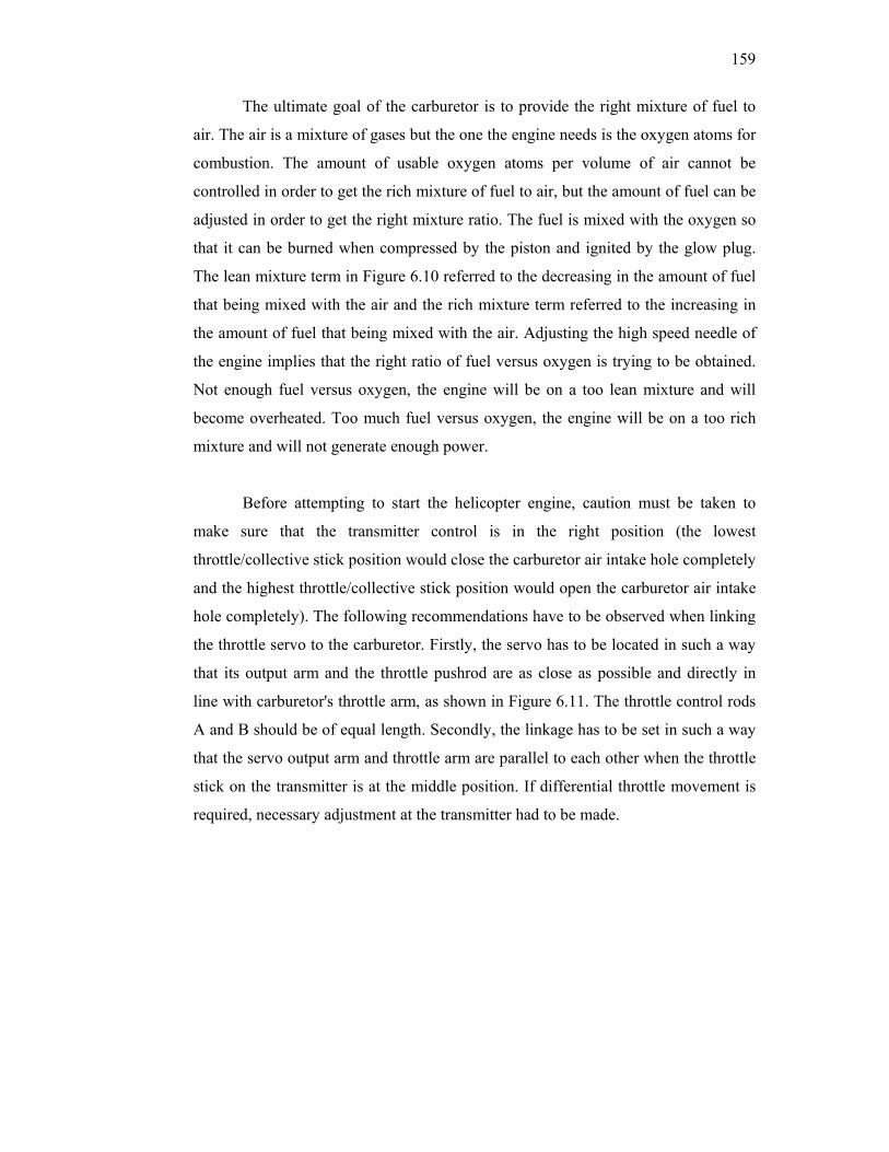
159
The ultimate goal of the carburetor is to provide the right mixture of fuel to
air. The air is a mixture of gases but the one the engine needs is the oxygen atoms for
combustion. The amount of usable oxygen atoms per volume of air cannot be
controlled in order to get the rich mixture of fuel to air, but the amount of fuel can be
adjusted in order to get the right mixture ratio. The fuel is mixed with the oxygen so
that it can be burned when compressed by the piston and ignited by the glow plug.
The lean mixture term in Figure 6.10 referred to the decreasing in the amount of fuel
that being mixed with the air and the rich mixture term referred to the increasing in
the amount of fuel that being mixed with the air. Adjusting the high speed needle of
the engine implies that the right ratio of fuel versus oxygen is trying to be obtained.
Not enough fuel versus oxygen, the engine will be on a too lean mixture and will
become overheated. Too much fuel versus oxygen, the engine will be on a too rich
mixture and will not generate enough power.
Before attempting to start the helicopter engine, caution must be taken to
make sure that the transmitter control is in the right position (the lowest
throttle/collective stick position would close the carburetor air intake hole completely
and the highest throttle/collective stick position would open the carburetor air intake
hole completely). The following recommendations have to be observed when linking
the throttle servo to the carburetor. Firstly, the servo has to be located in such a way
that its output arm and the throttle pushrod are as close as possible and directly in
line with carburetor's throttle arm, as shown in Figure 6.11. The throttle control rods
A and B should be of equal length. Secondly, the linkage has to be set in such a way
that the servo output arm and throttle arm are parallel to each other when the throttle
stick on the transmitter is at the middle position. If differential throttle movement is
required, necessary adjustment at the transmitter had to be made.
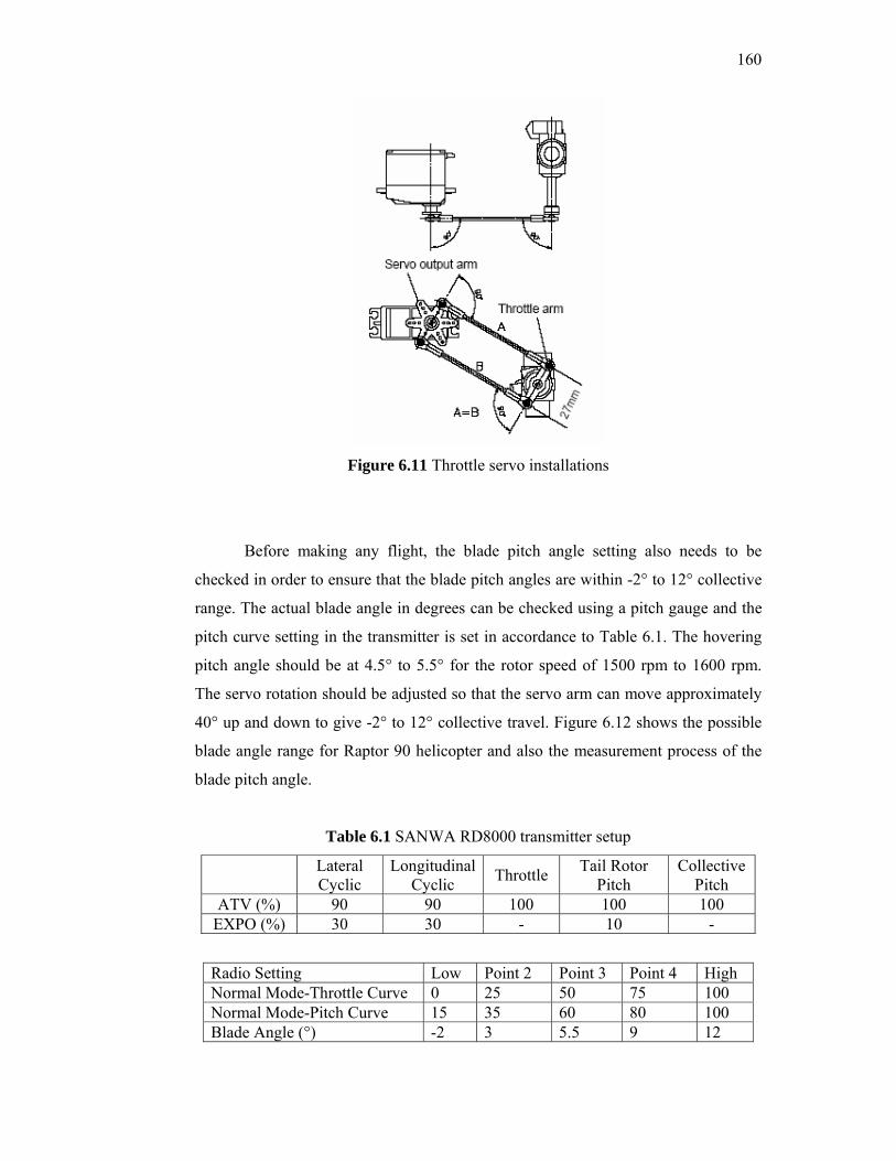
160
Figure 6.11 Throttle servo installations
Before making any flight, the blade pitch angle setting also needs to be
checked in order to ensure that the blade pitch angles are within -2° to 12° collective
range. The actual blade angle in degrees can be checked using a pitch gauge and the
pitch curve setting in the transmitter is set in accordance to Table 6.1. The hovering
pitch angle should be at 4.5° to 5.5° for the rotor speed of 1500 rpm to 1600 rpm.
The servo rotation should be adjusted so that the servo arm can move approximately
40° up and down to give -2° to 12° collective travel. Figure 6.12 shows the possible
blade angle range for Raptor 90 helicopter and also the measurement process of the
blade pitch angle.
Table 6.1 SANWA RD8000 transmitter setup
Lateral Cyclic
Longitudinal Cyclic Throttle Tail Rotor
Pitch Collective
Pitch ATV (%) 90 90 100 100 100
EXPO (%) 30 30 - 10 -
Radio Setting Low Point 2 Point 3 Point 4 High Normal Mode-Throttle Curve 0 25 50 75 100 Normal Mode-Pitch Curve 15 35 60 80 100 Blade Angle (°) -2 3 5.5 9 12

161
Figure 6.12 Blade pitch and collective travel setting
Blade tracking adjustment has also to be made if rotor blades were out of
track by adjusting one of the pushrods that connects to the main rotor blade pitch
arm. When the two main rotor blades are in track it means that the two blade tips
should follow the same path as they rotate. Figure 6.13 shows examples of the
possible blade tracking conditions, i.e. one out of and the other in tracks. If one of the
following symptoms was observed, i.e. blades track on one side only, tracking
changes in flight, tracking changes with cyclic input or helicopter pitchy in forward
flight, then the helicopter entire flybar system has to be checked thoroughly. The
flybar needs to be centered in the see saw hub and the flybar rod should be straight.
A straight edge ruler can be used for these purposes. Always do make sure that the
surfaces of the flybar, flybar paddles, swashplate and the top of metal frame are in
parallel to each other as shown in Figure 6.14.
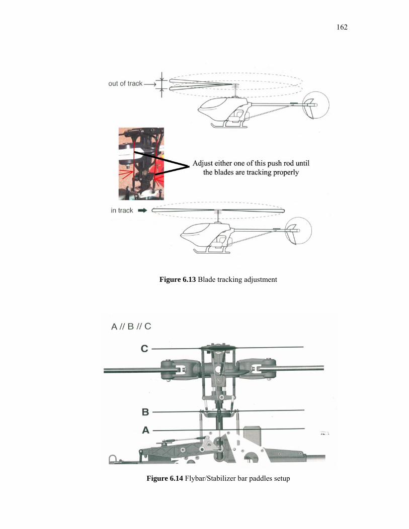
162
Figure 6.13 Blade tracking adjustment
Figure 6.14 Flybar/Stabilizer bar paddles setup
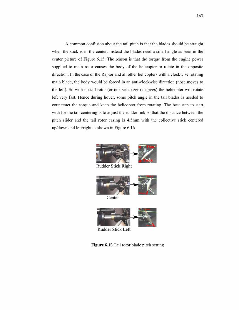
163
A common confusion about the tail pitch is that the blades should be straight
when the stick is in the center. Instead the blades need a small angle as seen in the
center picture of Figure 6.15. The reason is that the torque from the engine power
supplied to main rotor causes the body of the helicopter to rotate in the opposite
direction. In the case of the Raptor and all other helicopters with a clockwise rotating
main blade, the body would be forced in an anti-clockwise direction (nose moves to
the left). So with no tail rotor (or one set to zero degrees) the helicopter will rotate
left very fast. Hence during hover, some pitch angle in the tail blades is needed to
counteract the torque and keep the helicopter from rotating. The best step to start
with for the tail centering is to adjust the rudder link so that the distance between the
pitch slider and the tail rotor casing is 4.5mm with the collective stick centered
up/down and left/right as shown in Figure 6.16.
Figure 6.15 Tail rotor blade pitch setting
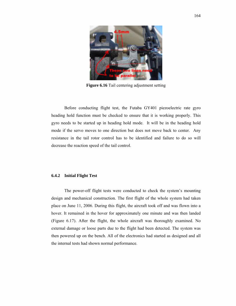
164
Figure 6.16 Tail centering adjustment setting
Before conducting flight test, the Futaba GY401 piezoelectric rate gyro
heading hold function must be checked to ensure that it is working properly. This
gyro needs to be started up in heading hold mode. It will be in the heading hold
mode if the servo moves to one direction but does not move back to center. Any
resistance in the tail rotor control has to be identified and failure to do so will
decrease the reaction speed of the tail control.
6.4.2 Initial Flight Test
The power-off flight tests were conducted to check the system’s mounting
design and mechanical construction. The first flight of the whole system had taken
place on June 11, 2006. During this flight, the aircraft took off and was flown into a
hover. It remained in the hover for approximately one minute and was then landed
(Figure 6.17). After the flight, the whole aircraft was thoroughly examined. No
external damage or loose parts due to the flight had been detected. The system was
then powered up on the bench. All of the electronics had started as designed and all
the internal tests had shown normal performance.

165
Figure 6.17 The Initial flight test
6.4.3 Partial Computer Controlled Flight
Partial computer controlled flight was when the pilot flew only one channel
of control (Collective pitch/Throttle) and the computer flew the remaining channels
(Figure 6.18). Most of the flight testing of the aircraft had been done in this mode.
The purpose of this flight testing was to allow for the tuning of the flight control
system, one channel at a time. The computer flew the longitudinal cyclic, lateral
cyclic and yaw channel. Once each channel was tuned up separately, the
combinations were then turned over to computer control. This type of flight testing
was done on a regular basis. During these testing, telemetry data was being used to
monitor the performance of the avionics while in flight. At no point during these
testing did any of the electronics fail while the aircraft was flying.
The experiment results of the hovering controller tested on the Raptor .90
helicopter model is shown in Figure 6.19, 6.20 and 6.21 for roll, pitch and yaw angle
stabilization. The UAV showed a stable attitude response over two minutes and
began to sway slowly from the current hovering position since the positional
controller is not implemented. The graph shows that the roll angle is regulated within
± 2°~3° (± 0.3049~0.0524 rad), pitch angle is within ± 3°~4° (± 0.0524~0.0698 rad)
while yaw angle is within ± 99°~103° (± 1.7279~1.7977 rad).

166
Figure 6.18 Partially computer control flight test
Figure 6.19 Experiment results of attitude (roll angle) regulation by autopilot system

167
Figure 6.20 Experiment results of attitude (pitch angle) regulation by autopilot system
Figure 6.21 Experiment results of attitude (yaw angle) regulation by autopilot system

168
6.5 Conclusion
This chapter describes the performance evaluation of autopilot system
developed through the tests conducted in test rig, preliminary test and actual flight
test. The proposed hovering controller has shown capable of stabilizing the
helicopter attitude angles. The positional, velocity and heave controller design could
not be implemented in the tests due to limitation of resources in this project. A GPS
device should be used as part of autopilot’s sensor to give position information to
flight computer. The combination of AHRS and GPS device could enable better
hovering stabilization control of helicopter model with position hold capabilities.
CHAPTER 5
SYSTEM INTEGRATION
5.1 Introduction
One of the main goals of this research project is to develop and establish a
comprehensive and practical methodology to design an UAV with a reliable accuracy
autopilot system. To demonstrate this idea, the vehicle platform should be integrated
with proper hardware and software so that the vehicle can perform the desired
autonomous maneuver.
5.2 Air Vehicle Descriptions
The basis of the UAV platform is a conventional model helicopter, the Raptor
.90 class RC Helicopter manufactured by Thunder Tiger Corporation, Taiwan
(Figure 5.1). It has a rotor diameter of 1.55m and is equipped with a high
performance OS MAX-91SX-HRING C SPEC PS (90 cu in) two-stroke
nitromethane engine which produces about 15kW of power with the practical RPM
ranges from 2000 to 16000. Raptor .90 class helicopter has an empty weight of about
7.7 kg, capable to carry about 3 kg payloads with an operation time of about 15
minutes.

111
Figure 5.1 Thunder Tiger Raptor .90 class helicopter equipped with two stroke nitromethane engine of 14.9 cc displacement
This helicopter consists of a fuselage, a main rotor, a tail boom/tail rotor
assembly and landing skid. The glow plug engine is mounted upside-down below the
transmission casing for compact design and can only be assessed from bottom, left or
behind. This prohibits the mounting of any avionic systems in this area and leaves
this vehicle less attractive for tight component installation. The engine is started by
first preheating the glow plug with a low-voltage high-current battery (typically
1.5V, 1500 mAH NiCad batteries) and then cranking the engine by applying a DC
motor starter to the starter-shaft coupling that rotates the engine crankshaft through
clutch bell set. The engine is designed to idle at about 2000 RPM, and as the RPM
increases towards its nominal value of about 10,000-11,000 RPM, the clutch at the
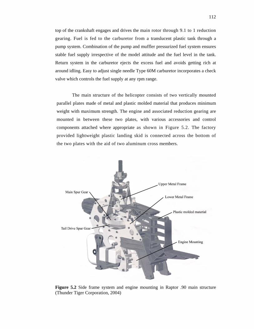
112
top of the crankshaft engages and drives the main rotor through 9.1 to 1 reduction
gearing. Fuel is fed to the carburetor from a translucent plastic tank through a
pump system. Combination of the pump and muffler pressurized fuel system ensures
stable fuel supply irrespective of the model attitude and the fuel level in the tank.
Return system in the carburetor ejects the excess fuel and avoids getting rich at
around idling. Easy to adjust single needle Type 60M carburetor incorporates a check
valve which controls the fuel supply at any rpm range.
The main structure of the helicopter consists of two vertically mounted
parallel plates made of metal and plastic molded material that produces minimum
weight with maximum strength. The engine and associated reduction gearing are
mounted in between these two plates, with various accessories and control
components attached where appropriate as shown in Figure 5.2. The factory
provided lightweight plastic landing skid is connected across the bottom of
the two plates with the aid of two aluminum cross members.
Figure 5.2 Side frame system and engine mounting in Raptor .90 main structure (Thunder Tiger Corporation, 2004)
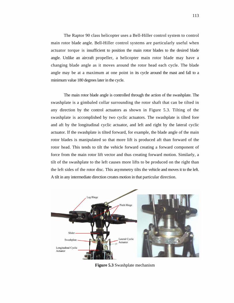
113
The Raptor 90 class helicopter uses a Bell-Hiller control system to control
main rotor blade angle. Bell-Hiller control systems are particularly useful when
actuator torque is insufficient to position the main rotor blades to the desired blade
angle. Unlike an aircraft propeller, a helicopter main rotor blade may have a
changing blade angle as it moves around the rotor head each cycle. The blade
angle may be at a maximum at one point in its cycle around the mast and fall to a
minimum value 180 degrees later in the cycle.
The main rotor blade angle is controlled through the action of the swashplate. The
swashplate is a gimbaled collar surrounding the rotor shaft that can be tilted in
any direction by the control actuators as shown in Figure 5.3. Tilting of the
swashplate is accomplished by two cyclic actuators. The swashplate is tilted fore
and aft by the longitudinal cyclic actuator, and left and right by the lateral cyclic
actuator. If the swashplate is tilted forward, for example, the blade angle of the main
rotor blades is manipulated so that more lift is produced aft than forward of the
rotor head. This tends to tilt the vehicle forward creating a forward component of
force from the main rotor lift vector and thus creating forward motion. Similarly, a
tilt of the swashplate to the left causes more lifts to be produced on the right than
the left sides of the rotor disc. This asymmetry tilts the vehicle and moves it to the left.
A tilt in any intermediate direction creates motion in that particular direction.
Figure 5.3 Swashplate mechanism
114
The collective actuator moves the swashplate up and down the rotor shaft and
does not induce any tilt to the swashplate. As the swashplate moves up, blade
angle is increased by the same amount at all points through the cycle. This creates a
uniform increase in lift across the disc with an overall increase in lifting force.
The process by which swashplate tilt creates an uneven lift distribution
is a complicated one, as it involves the effects of gyroscopic precession. If a force is
applied to a toy gyroscope for example, deflection occurs at a 90 degree angle from
the direction of the applied force. For a rotating airfoil, the effects of a change in
an airfoil's angle-of-attack (AOA) appear as a change in airfoil lift 90 degrees later in the
cycle.
In addition to the two large main rotor blades, two small airfoils called servo
paddles are installed at the ends of a flybar at right angles to the two main rotor blades.
All these four airfoils are subjected to gyroscopic effects. In the case of the main rotor
blades, the linkage from the swashplate causes the blade angle to be increased 90
degrees prior to the point in the cycle when it is needed (Shim, 2000). For example,
if the swashplate were to be tilted forward, blade angle reaches a maximum on the
starboard side of the cycle, and a minimum at the port side of the cycle. As the
rotor turns clockwise when viewed from above, lift is increased aft and decreased
forward, creating the desired asymmetry.
The servo paddles serve to assist in twisting the blades to their new positions,
since the actuators lack sufficient torque on their own. The AOA of one paddle is
increased by a linkage from the swashplate, while the AOA of the other paddle is
decreased. Since the flybar joining the paddles is free to rotate in the vertical plane at
the head block, the flybar can move in a seesaw motion. This seesaw motion causes the
main rotor blade angle to change through a connecting linkage (Greer, 1998).
The gyroscopic effect on the servo paddles must be considered. In our example
of forward swashplate tilt, the linkage to the servo paddles increases AOA of
the paddles to a maximum as passing the right side of the mast. The effect of the lift
produced on the paddle is felt 90 degrees later, at which point the flybar seesaws. The

115
seesaw motion increases blade angle of attack of the blade located on the starboard
side. This increase in lift appears 90 degrees later when the blade is aft of the rotor, thus
creating the desired asymmetry of lift. The basic principle of operation of the rotor
control is to give the main rotor a following rate which is compatible with normal
pilot responses. The following rate is the rate at which the tip path plane of main
rotor follows the control stick movements made by the pilot or realigns itself with the
mast after an aerodynamics disturbance.
A total of four electrically powered Hitec HS945 MG and one Futaba S-9254
actuators or control servos are used to position throttle, collective, lateral cyclic,
longitudinal cyclic and tail rotor linkages. A small rechargeable 4.8V Type C 2000
mAH battery provides power to the actuators through a SANWA RX-611
Remote Control (RC) receiver located in front of servo frame. This 40 MHz crystal
receiver is tuned to a frequency corresponding to RC channel 51. The receiver
processes signals transmitted by a hand-held SANWA RD8000 transmitter on the
ground and produces Pulse Width Modulated (PWM) output signals to drive the
servos. The receiver may accommodate as many as 5 different actuators but after
several modifications made to the standard receiver circuit, the receiver is able to
control up to 7 different actuators. SANWA has provided 2 extra pin on its receiver
Static Shift Register chip for extra channel. The CMOS Dual 4 stage Static Shift
Register chip from Intersil Corporation used in the design of SANWA RX-611
receiver can be identified through the CD4015BMS marking on the back of the
receiver circuit. The channel assignments are shown in Table 5.1.
Table 5.1 Helicopter PWM receiver output channels
Receiver Channel Output
1 Longitudinal Cyclic (Front/Aft movement)
2 Lateral Cyclic (Left/Right movement)
3 Throttle
4 Tail Rotor/Gyro
5 Rate Gyro Sensitivity Switching
6 Collective Pitch
7 Power Supply
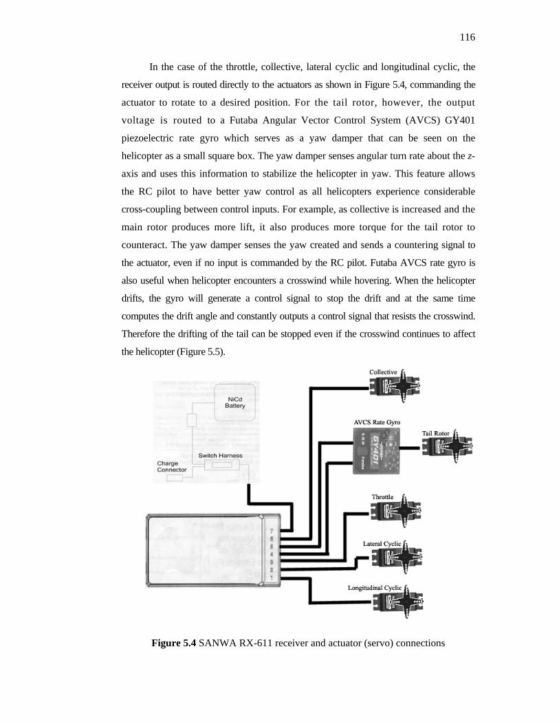
116
In the case of the throttle, collective, lateral cyclic and longitudinal cyclic, the
receiver output is routed directly to the actuators as shown in Figure 5.4, commanding the
actuator to rotate to a desired position. For the tail rotor, however, the output
voltage is routed to a Futaba Angular Vector Control System (AVCS) GY401
piezoelectric rate gyro which serves as a yaw damper that can be seen on the
helicopter as a small square box. The yaw damper senses angular turn rate about the z-
axis and uses this information to stabilize the helicopter in yaw. This feature allows
the RC pilot to have better yaw control as all helicopters experience considerable
cross-coupling between control inputs. For example, as collective is increased and the
main rotor produces more lift, it also produces more torque for the tail rotor to
counteract. The yaw damper senses the yaw created and sends a countering signal to
the actuator, even if no input is commanded by the RC pilot. Futaba AVCS rate gyro is
also useful when helicopter encounters a crosswind while hovering. When the helicopter
drifts, the gyro will generate a control signal to stop the drift and at the same time
computes the drift angle and constantly outputs a control signal that resists the crosswind.
Therefore the drifting of the tail can be stopped even if the crosswind continues to affect
the helicopter (Figure 5.5).
Figure 5.4 SANWA RX-611 receiver and actuator (servo) connections

117
Figure 5.5 The gyro automatically corrects changes in the helicopter tail trim by crosswind (FUTABA Corporation, 2003)
The SANWA RD8000 hand-held transmitter shown in Figure 5.6
contains two primary levers for vehicle control. The up-down movement of the
right lever controls the throttle and collective pitch while left-right movement control
the lateral cyclic. Left-right motion of the left lever of the transmitter controls the
tail rotor, while up-down motion simultaneously controls the longitudinal cyclic.
The SANWA RD8000 transmitter features mixing capabilities that adjust the tail
rotor to roughly compensate for the change in torque created as the throttle and
collective pitch increase. The RD8000 transmitter also has the capability that
allows us to connect any two SANWA RD series transmitter together for the
purpose of training a new pilot. In actual use, one of the two transmitters is held
by the instructor pilot (Master Transmitter) and the second transmitter will serve
as the Trainer Transmitter. As long as the instructor holds his trainer switch in the
ON position, the model will respond to the commands of the trainer transmitter
sticks allowing the student to fly the model. The Master Transmitter will have full
control of the model if the trainer switch on the instructor’s transmitter is left in its
OFF position.
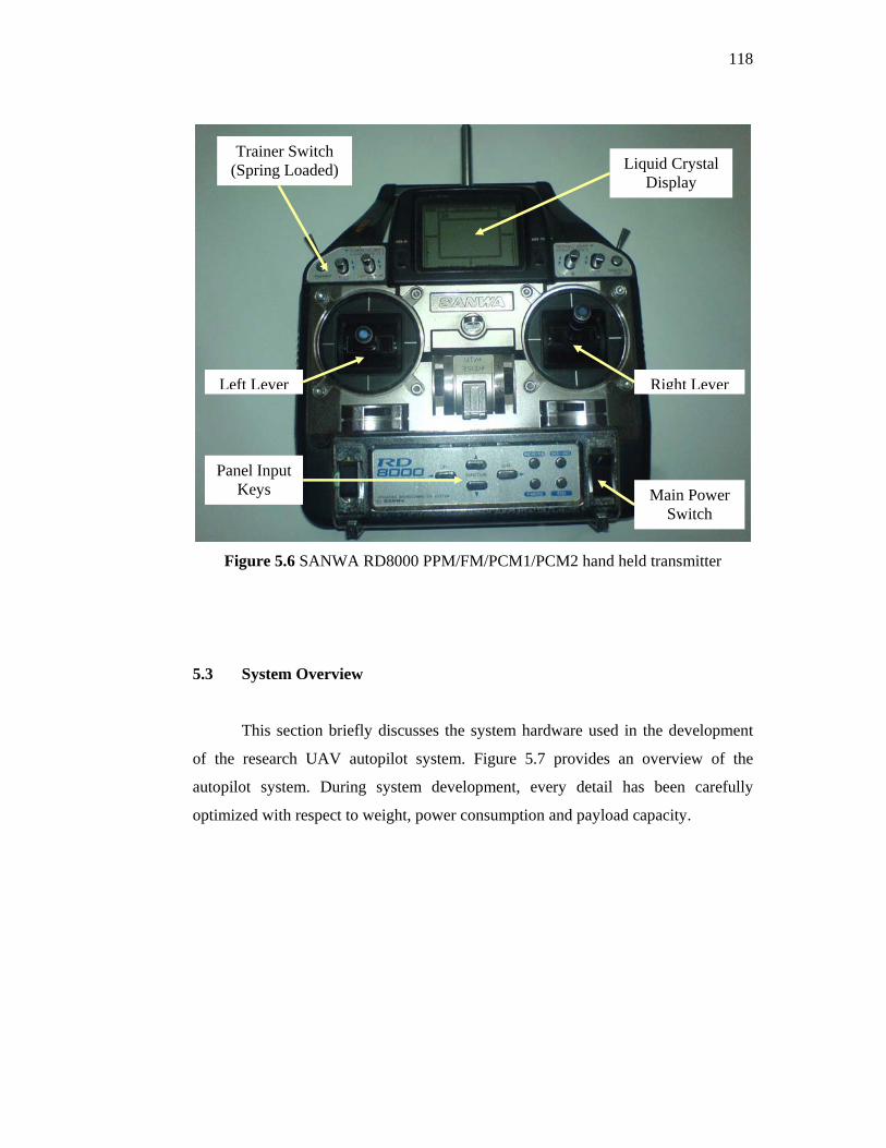
118
Figure 5.6 SANWA RD8000 PPM/FM/PCM1/PCM2 hand held transmitter
5.3 System Overview
This section briefly discusses the system hardware used in the development
of the research UAV autopilot system. Figure 5.7 provides an overview of the
autopilot system. During system development, every detail has been carefully
optimized with respect to weight, power consumption and payload capacity.
Trainer Switch (Spring Loaded)
Right LeverLeft Lever
Panel Input Keys Main Power
Switch
Liquid Crystal Display
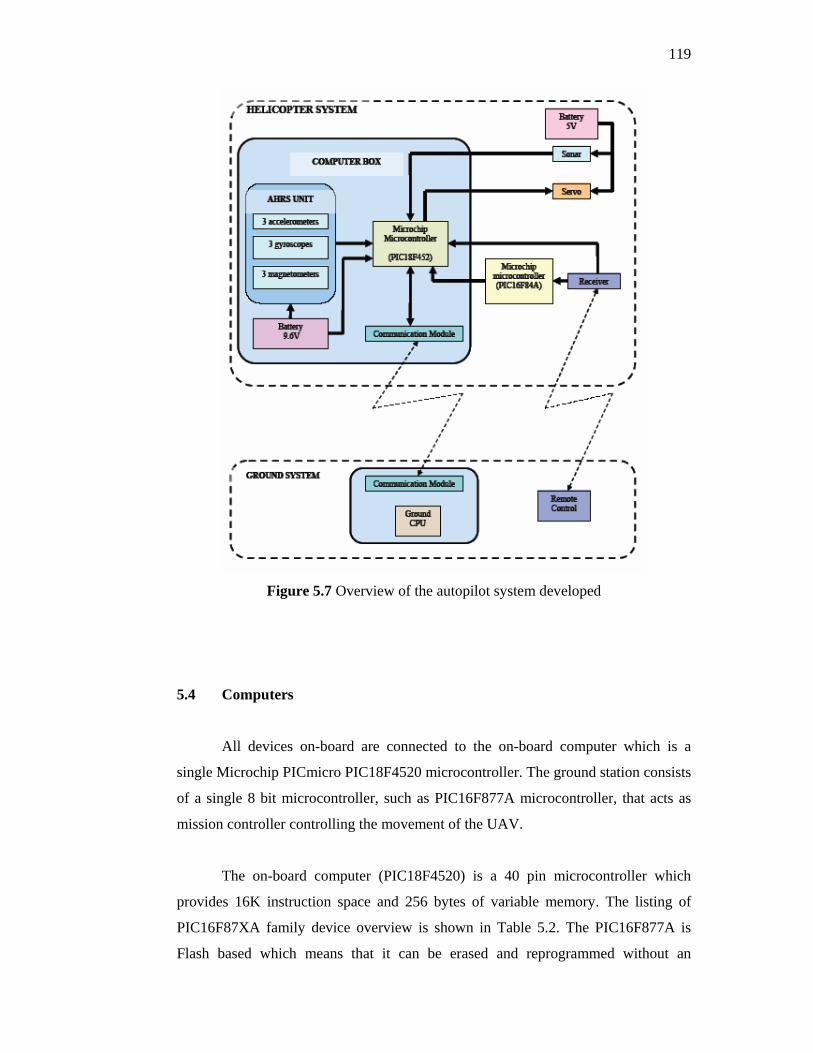
119
Figure 5.7 Overview of the autopilot system developed
5.4 Computers
All devices on-board are connected to the on-board computer which is a
single Microchip PICmicro PIC18F4520 microcontroller. The ground station consists
of a single 8 bit microcontroller, such as PIC16F877A microcontroller, that acts as
mission controller controlling the movement of the UAV.
The on-board computer (PIC18F4520) is a 40 pin microcontroller which
provides 16K instruction space and 256 bytes of variable memory. The listing of
PIC16F87XA family device overview is shown in Table 5.2. The PIC16F877A is
Flash based which means that it can be erased and reprogrammed without an

120
ultraviolet light source, and can be reprogrammed just using a simple programmer
circuit. Figure 5.8 shows the pin diagram of PIC18F4520 and the pinout descriptions
of PIC18F4520 for each port are shown in Appendix D.
Table 5.2 The PIC18F2420/2520/4420/4520 family device overview (Microchip Technology Inc, 2004)
Figure 5.8 The pinout diagram of PIC18F4520 microcontroller (Microchip Technology Inc, 2004)

121
5.4.1 PIC Microcontroller Programming Overview
Programming PIC microcontroller is a simple three steps process: write the
code, compile the code and upload the code into the microcontroller. In this research,
code writing and code compilation were done using PICBasic PRO Compilers. The
PicBasic Pro Compiler makes it even quicker and easier to program Microchip
Technology’s powerful PIC microcontrollers. The English-like BASIC language is
much easier to read and write than the Microchip assembly language. The PICBasic
Pro Compiler IDE screen shot is shown in Figure 5.9.
Figure 5.9 Screen shot of PICBasic Pro Compiler IDE
The current version of the PicBasic Pro Compiler supports most of the
Microchip Technology PICmicro microcontroller units, including the 12-bit core, 14-
bit core, both 16-bit core series, the PIC17Cxxx and PIC18Xxxx devices, and as well

122
as the Micromint PicStics. Limited support has been added to the PIC
microcontroller units based on the original 12-bit core since these microcontroller
units have a limited set of resources including a smaller stack and a smaller code
page size.
For general purpose PIC microcontroller unit (MCU) development using the
PicBasic Pro Compiler, the PIC12F675, 16F648A, 16F84, 16F876, 16F877, 18F252
and 18F452 are the current PIC microcontroller units of choice. These
microcontrollers use flash technology to allow rapid erasing and reprogramming to
speed up program debugging. With the click of the mouse in the programming
software, the flash PICmicro MCU can be instantly erased and then reprogrammed
again and again. Other PICmicro microcontroller units in the PIC12C5xx, 12C67x,
14000, 16C4xx, 16C5x, 16C55x, 16C6xx, 16C7xx, 16C9xx, 17Cxxx and 18Cxxx
series are either one-time programmable (OTP) or have a quartz window in the top
(JW) to allow erasure by exposure to ultraviolet light for several minutes. Most
PIC12F6xx, 16F6xx, 16F8xx and 18Fxxx devices also contain between 64 and 1024
bytes of non-volatile data memory that can be used to store program data and other
parameters even when the power is turned off. This data area can be accessed simply
by using the PicBasic Pro Compiler’s READ and WRITE commands.
The next item needed in the programming of a microcontroller is the PIC
programmer. The PIC programmer consists of software and a programming carrier
board (hardware). It is the programmer hardware and software that the compiled .hex
file generated by the compiler and uploads it into the microcontroller where it may
run. It can be purchased from a number of distributors such as microEngineering
Labs, Ltd, Microchip Technology, Ltd, Custom Computer Services, Ltd., B Knudsen
Data and Byte Craft Limited.
The flowchart for the autopilot programming can be viewed in Figure 5.10.
The flowchart shows the flow of instruction execution made in performing automatic
attitude stabilization and manual-automatic control switching. Note that in absolute
testing routine, the updated AHRS reading will be compared to initial AHRS reading
to determine the movement correction required to stabilize the helicopter in hovering

123
flight as shown in Figure 5.11. PICBasic codes for automatic attitude stabilization
and manual-automatic control switching are given in Appendix C.
Figure 5.10 PicBasic Pro programming flowchart in roll attitude stabilization. Similar programming flow is used for pitch and yaw attitude stabilization.
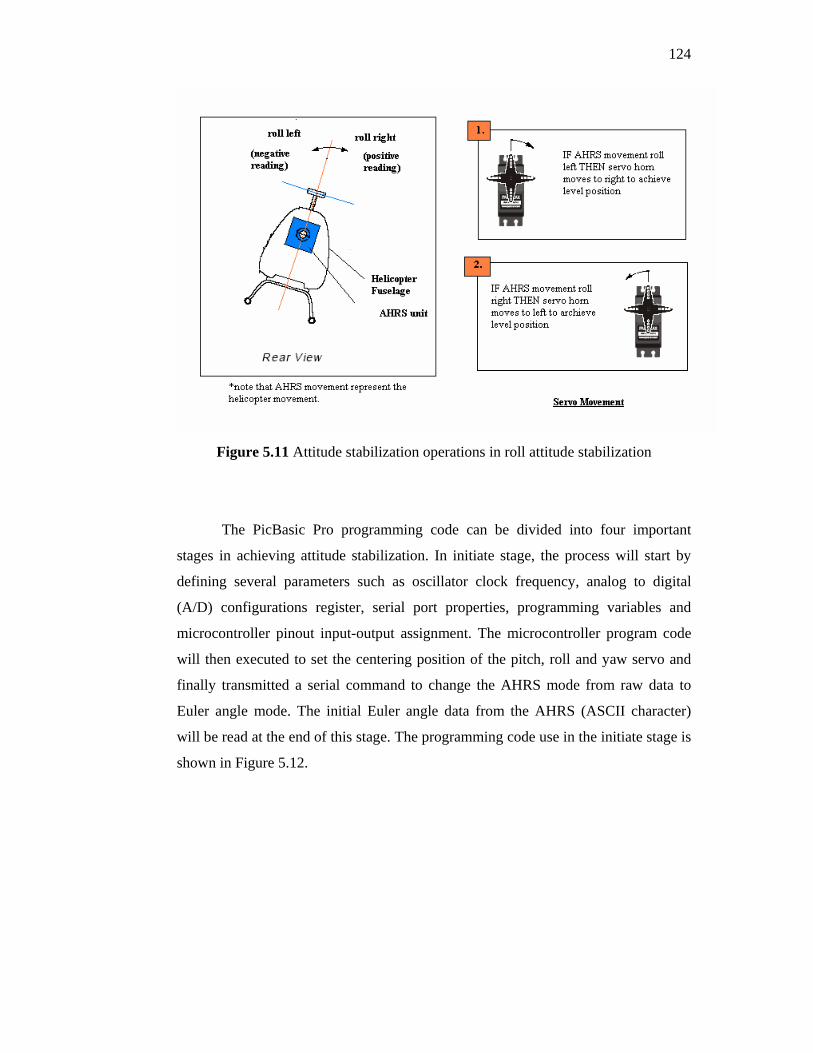
124
Figure 5.11 Attitude stabilization operations in roll attitude stabilization
The PicBasic Pro programming code can be divided into four important
stages in achieving attitude stabilization. In initiate stage, the process will start by
defining several parameters such as oscillator clock frequency, analog to digital
(A/D) configurations register, serial port properties, programming variables and
microcontroller pinout input-output assignment. The microcontroller program code
will then executed to set the centering position of the pitch, roll and yaw servo and
finally transmitted a serial command to change the AHRS mode from raw data to
Euler angle mode. The initial Euler angle data from the AHRS (ASCII character)
will be read at the end of this stage. The programming code use in the initiate stage is
shown in Figure 5.12.

125
Figure 5.12 Code fragment used in the initiate stage
In the Switching stage, the manual to automatic switching is implemented by
determining either bit logic received by digital input pin B7 is high (+5V) or low (0
V). If the input is high, the program code will jump to manual mode where the
PIC18F4520 microcontroller’s port B is set to be equivalent with port D which
enables direct control of helicopter servo via the receiver. Figure 5.13 show the
programming code in the switching stage.

126
Figure 5.13 Code fragment used in the switching stage
The process will continue in the automatic mode if the condition satisfied and
proceed to testing stage. In this stage, the program will start to calculate and convert
the ACSII character (Euler angle data output) transmitted by AHRS into meaningful
decimal value. The decimal value is then tested for it absolute value and sign
representations (negative of positive value). The routine for testing stage can be
referred in Appendix C.
The process will continue to execution stage where updated data reading is
compared to initial data reading. A simple logic statement will be used to determine
the desired servo movements. The routine will then generated a PWM signal
acquired to move the servo based on the decision made by logic statement. The
controller gain values determined in previous chapter can also be used to fine tune
the servo movement in order to achieve the desired control performance. Note that
the PWM signal generated will have to be limited at the servo maximum or
minimum traveling value in order to prevent damage to servo gearing mechanism.
Figure 5.14 show the programming code in the execution stage.

127
Figure 5.14 Code fragment used in the execution stage

128
5.5 Sensors
Avionics system sensors are needed to collect information on how the aircraft
and control systems are performing. Kahn (2001) has suggested that for a basic UAV
flight control avionics package, three major sensor systems are needed namely the
attitude and heading system, the position and velocity system and the altitude system.
These three sensor systems are needed to measure the basic states of the aircraft
requiring for flight control. Due to limitation in the research funding, the Global
Positioning System (GPS) for position and velocity determination cannot be
implemented into our avionic system since it is too costly.
Attitude determination of a UAV is critical if flight is to be maintained. There
are two major ways to maintain the attitude of a UAV (Kahn, 2001). The first
method is to use a sensor system called an attitude and heading reference system
(AHRS). This device is a fully integrated sensor that can determine the attitude,
magnetic heading and attitude rates of the vehicle. An AHRS system is limited in its
maximum tilt due to the internal operation of the sensor. Both analog and digital
outputs from this type of sensor are available, but digital is more common. The
industry is using RS-232 serial communications for the digital output. The second
attitude system is an aided inertial navigation system (INS). This attitude
measurement system is very accurate and has higher limits than the AHRS but it is
difficult and more expensive to implement. Past systems of this type were built of
separate components and then integrated on the aircraft in a closed fashion. Newer
technology has allowed this type of sensor to be built into a single device. The cost
comparison between an integrated aided INS and an AHRS is dramatic. The aided
INS system is substantially more expensive than an AHRS device.
For autopilot system developed in this project, an AHRS has been selected
for UAV attitude measurement using Rotomotion low-dynamics Attitude and
Heading Reference System (AHRS3050AA) consisting of a six degree of freedom
inertial measurement unit (6-DOF IMU) and a three axis magnetometer for heading
measurement. The Kalman filter used in this product will track 16 states consisting of
Euler angles (φ ,θ ,ψ ), orientation in quaternion (q0, q1, q2, q3), angular rate or gyro

129
biases (p, q, r ), magnetic fields (mx, my, mz) and accelerations (ax, ay, az). Figure 5.15
shows the AHRS purchased from Rotomotion, LLC. The AHRS outputs ASCII data
on its serial port at 38400 baud (N81) with no flow control. The ASCII can be view
with Minicom or HyperTerminal depending on the application. The AHRS user
guide details how to select output format by typing various symbol and command
(Rotomotion, 2004). Each line consists of a marker indicating the type of data and a
comma separating list of values. An important consideration when determining how
to mount the AHRS unit on the helicopter is the orientation of the axes of the AHRS.
The arrow in Figure 5.15 shows the direction where the AHRS unit should be
pointed at in order to align the AHRS coordinates with the conventional aircraft
coordinate system. Additionally, to ensure that the internal magnetometers are not
influence by disturbances, care should be given to use non-magnetic mounting
materials and non-magnetic electrical connections. The AHRS3050AA specification
summaries are shown in Table 5.3.
Figure 5.15 The low dynamic AHRS (AHRS3050AA) from Rotomotion, LLC. This AHRS operates at slower updated rated (30Hz) and output the attitude measurement via serial port compare to other high end AHRS from Rotomotion, LLC.
Forward-Aircraft Nose

130
Table 5.3 Rotomotion AHRS3050AA specifications
Specifications
Item Unit Condition Specification
Maximum detectable angular rate (deg/sec) 25 °C +/- 90
Maximum detectable acceleration rate (m/s2) +/- 19.6
Roll/Pitch Precision (°) 0.5
Heading Precision (°) 1
AHRS State Update Rate (Hz) 50Hz Quaternion
30Hz Euler Angles
Supply voltage (V) +7.2 to +24.0
Current consumption (mA)
max. 7.2V 80
Operating temp range (C) -5 to 75
Storage temp range (C) -40 to 80
The final component is the altitude measurement system. Although GPS can
provide altitude information, this data contains no information about what is below
the aircraft. If the UAV is to take-off and land under computer control, it is then
required to have some knowledge of how high the vehicle is above the ground. There
are several common ways to measure altitude including the using of radar, sonar, and
lidar altimeter (Kahn, 2001). Radar and lidar altimeters are both fairly expensive
components compared to a sonar system, but having a much greater range than sonar.
The data for all these types of altimeters are available in RS-232 format.
For the purpose of this research work, a Polaroid 6500 sonar ranging module
from SensComp (Figure 5.16) has been chosen. The 6500 Series is an economical
sonar ranging module that can drive all SensComp/Polaroid electrostatic transducers
with no additional interface. This module, with a simple interface, is able to measure
distances from 6 inches to 35 feet (0.1524m to 10.668m). The typical absolute
accuracy is ± 1% of the reading over the entire range.

131
This module has an external blanking input that allows selective echo
exclusion for operation on a multiple-echo mode. The module is able to differentiate
echoes from objects that are only three inches apart. The digitally controlled-gain,
variable-bandwidth amplifier minimizes noise and side-lobe detection in sonar
applications.
The module has an accurate ceramic-resonator-controlled 420-kHz time-base
generator. An output based on the 420-kilohertz time base is provided for external
use. The sonar transmit output is 16 cycles at a frequency of 49.4 kilohertz. The
6500 Series module operates over a supply range of 4.5 volts to 6.8 volts and is
characterized for operation from 0° C to 40° C.
Figure 5.16 The Polaroid 6500 Ranging module from SensComp
6500 sonar board
7000 Series Transducer Cable Connector

132
5.6 Communications
Communication between the helicopter and the ground station is performed
via wireless data link from LPRS EasyRadio ER400TRS module which operates at
433-4MHz. The CM02 module, together with its companion RF04 module forms a
complete interface between onboard computer and ground station. The wireless
module offers two ways communication which enables the user to send commands to
helicopter onboard computer and receive telemetry data from onboard sensors.
Figure 5.17 shows the telemetry pair (CM02 and RF04 modules) used in the research
project.
Figure 5.17 The RF04 and CM02 modules used in the research project
The EasyRadio ER400TRS Transceiver module is a complete sub-system that
combines a high performance very low power RF transceiver, a microcontroller and
a voltage regulator (Figure 5.18). The Serial Data Input and Serial Data Output
operate at the standard 19,200 Baud and the two handshake lines provide optional
flow control to and from the host. The Easy-Radio Transceiver can accept and
transmit up to 180 bytes of data, which it buffers internally before transmitting in an
efficient over-air code format. The pinout diagram of EasyRadio ER400TRS
transceiver is given in Table 5.4.

133
Figure 5.18 Easy Radio transceiver block diagram
Table 5.4 EasyRadio ER400TRS transceiver pinout diagram (Low Power Radio Solutions, 2005)
The EasyRadio ER400TRS transceiver module operates from an on board
3.3V low drop regulator. The logic levels of the input/output pins are therefore
between 0V and 3.3V. The serial inputs and outputs are intended for connection to a
UART or similar low logic device. A typical connection to RS232 port via MAX232
interface (Figure 5.19) can be used in order to ensure that the transceiver module is
not been damage by the voltages (+/- 12V) present on RS232 signal line.

134
Figure 5.19 MAX232 application circuit (Low Power Radio Solutions, 2005)
Figure 5.20 shows a typical system block diagram comprising hosts (users’
application) connected to Easy-Radio Transceivers. The hosts (A & B) will be
monitoring (collecting data) and/or controlling (sending data) to some real world
application. The hosts provide serial data input and output lines and two
‘handshaking’ lines that control the flow of data to and from the Easy-Radio
Transceivers. The ‘Busy’ output line, when active, indicates that the transceiver is
undertaking an internal task and is not ready to receive serial data. The ‘Host Ready’
input is used to indicate that the host is ready to receive the data held in the buffer of
the Easy-Radio Transceiver. The host should check before sending data that the
‘Busy’ line is not high, as this would indicate that the transceiver is either
transmitting or receiving data over the radio link. He should also pull the ‘Host
Ready’ line low and check that no data appears on the Serial Data Output line.
Figure 5.20 Typical system block diagram (Low Power Radio Solutions, 2005)
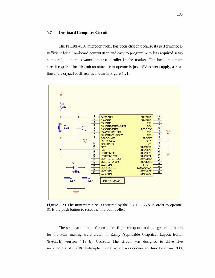
135
5.7 On-Board Computer Circuit
The PIC18F4520 microcontroller has been chosen because its performance is
sufficient for all on-board computation and easy to program with less required setup
compared to more advanced microcontroller in the market. The basic minimum
circuit required for PIC microcontroller to operate is just +5V power supply, a reset
line and a crystal oscillator as shown in Figure 5.21.
Figure 5.21 The minimum circuit required by the PIC16F877A in order to operate. S1 is the push button to reset the microcontroller.
The schematic circuit for on-board flight computer and the generated board
for the PCB making were drawn in Easily Applicable Graphical Layout Editor
(EAGLE) version 4.13 by CadSoft. The circuit was designed to drive five
servomotors of the RC helicopter model which was connected directly to pin RD0,
PIC18F4520
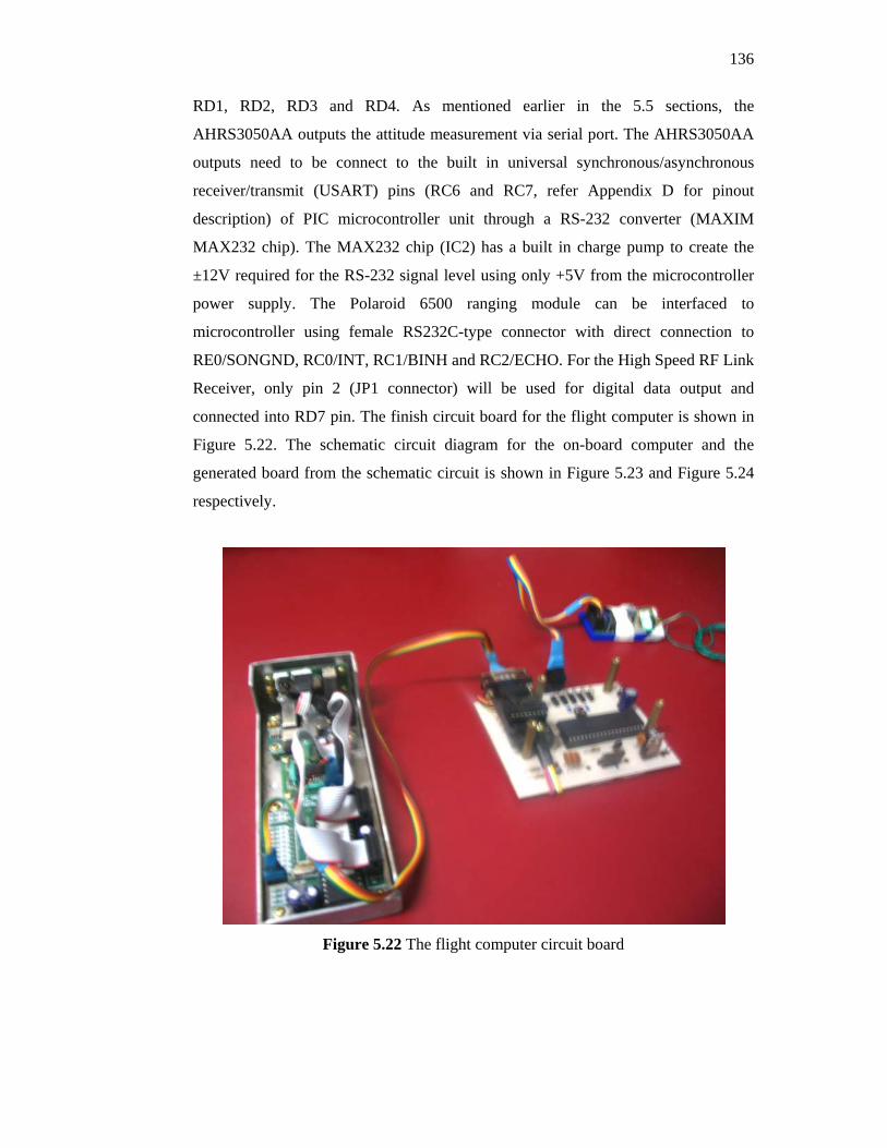
136
RD1, RD2, RD3 and RD4. As mentioned earlier in the 5.5 sections, the
AHRS3050AA outputs the attitude measurement via serial port. The AHRS3050AA
outputs need to be connect to the built in universal synchronous/asynchronous
receiver/transmit (USART) pins (RC6 and RC7, refer Appendix D for pinout
description) of PIC microcontroller unit through a RS-232 converter (MAXIM
MAX232 chip). The MAX232 chip (IC2) has a built in charge pump to create the
±12V required for the RS-232 signal level using only +5V from the microcontroller
power supply. The Polaroid 6500 ranging module can be interfaced to
microcontroller using female RS232C-type connector with direct connection to
RE0/SONGND, RC0/INT, RC1/BINH and RC2/ECHO. For the High Speed RF Link
Receiver, only pin 2 (JP1 connector) will be used for digital data output and
connected into RD7 pin. The finish circuit board for the flight computer is shown in
Figure 5.22. The schematic circuit diagram for the on-board computer and the
generated board from the schematic circuit is shown in Figure 5.23 and Figure 5.24
respectively.
Figure 5.22 The flight computer circuit board

137
Figure 5.23 Schematic design of on-board computer drawn in EAGLE version 4.13 by CadSoft

138
Figure 5.24 Generated board from schematic circuit drawn in EAGLE version 4.13 by CadSoft
5.8 System Integration
The basic helicopter used in this research does not provide any cargo area or
suitable enclosure to house the avionics suite. A platform of sufficient size to carry the
necessary components with a large margin for future growth is needed. Factors that
influenced the ultimate design of the avionics platform are:
i. The physical volume needed to mount the equipment,
ii. The need to place the AHRS on the centerline as near to the CG as possible,
iii. Weight and structural strength, and
iv. Ease of construction and availability of the materials.

139
The complete autopilot system integration with the helicopter can only be done
after all the electronics were built and installed. The following sections describe some
important issues during the integration process.
5.8.1 Power Systems
The power supply systems are an important aspect of the whole system. The
power supply to the system should be able to regulate some central voltage and deliver
the correct voltage to individual devices. Since the Polaroid 6500 ranging unit draws 2A
current during the short transmit period, the power supply from main board cannot be
used to handle the current in rush. This may cause voltage sag leading to microcontroller
reset. The solutions are to provide the units with a different 5V power supply or using 3
voltage regulators (LM7805) arranged in series to avoid microcontroller reset. In the
system presented, the main controller and the AHRS controller required 5V of power
supply and both devices will be using the same power supply from 9.6V NiCad
batteries. Both Polaroid 6500 ranging unit and helicopter servomotors will be sharing the
same power supply from 4.8V NiCad batteries.
5.8.2 Mounting
Any mounting design for an avionics system needs to be strong, light and allows
for easy removal of the systems. The main avionic box is designed and mounted in
between the helicopter engine and the landing skid as shown in Figure 5.25. The
helicopter is lifted about 9 cm from its datum using frame spacer in order to give space
to avionic platform. In the design for UTM autonomous helicopter, ¾” aluminum angle
plate was used to form the base structure. The two upper aluminum angle plates were
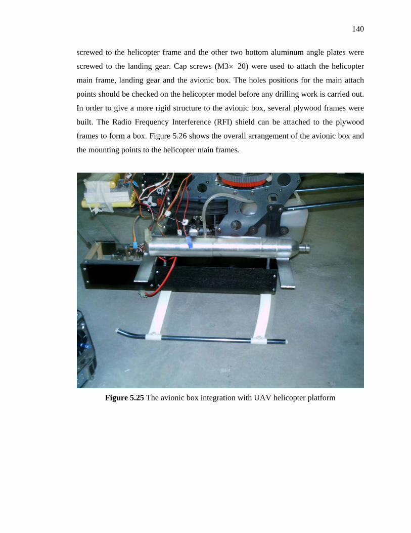
140
screwed to the helicopter frame and the other two bottom aluminum angle plates were
screwed to the landing gear. Cap screws (M3× 20) were used to attach the helicopter
main frame, landing gear and the avionic box. The holes positions for the main attach
points should be checked on the helicopter model before any drilling work is carried out.
In order to give a more rigid structure to the avionic box, several plywood frames were
built. The Radio Frequency Interference (RFI) shield can be attached to the plywood
frames to form a box. Figure 5.26 shows the overall arrangement of the avionic box and
the mounting points to the helicopter main frames.
Figure 5.25 The avionic box integration with UAV helicopter platform

141
Figure 5.26 The avionic box design and the mounting points to helicopter main frames
5.8.3 Component Placement
Placement of components on the avionic box was primarily influenced by weight
and balance considerations. An overhead view of the placement of components in the
avionic box is shown in Figure 5.27. The Attitude Heading Reference System (AHRS) is
a small black box that provides the computer with attitude, heading and angular rates for
flight control. This unit is designed to detect angles and angular rates. If the AHRS unit
is not mounted correctly, vibration can cause the unit to rotate. This rotation produces
noise especially in the rate channel. In order to prevent this, it is important to mount the
unit as close as possible to the predicted center of gravity (CG) and aligns to the aircraft
coordinate system. Figure 5.28 shows the plywood frames used to hold the AHRS from
any rotational movement. Batteries unit was placed at the helicopter servo frame while
¾” Aluminum Angle
Spacer
RFI Shields
Plywood Frames

142
autopilot circuit, telemetry unit, sonar circuitry and transducer were placed in the
forward portion of the avionic box.
Figure 5.27 Component placements in the avionic box
Figure 4.28 AHRS mounting design
Plywood Structure
AHRS Unit
AHRS UnitAutopilot

143
The center of gravity was tracked using a spreadsheet program which recorded
component position and weight (Table 5.5). The system used for recording positions is
similar to the practice used in full-size aircraft. The leading edge of the avionic box was
used as a datum from which fuselage stations were measured aft in meters and the
vertical measurements were taken from the ground (positive upwards). Lateral
measurements were taken from the centerline of the helicopter model (positive towards
starboard side). As shown in Table 5.5, the center of gravity is located directly below the
rotor mast (rotor head) at a point located 0.315 m aft of the leading edge and 0.235m
above the ground. The moment at the mast was found to be 0.774 Nm and the term
“moment at the mast” is referred to as the moment that must be generated by the rotor to
maintain longitudinal stability. The spreadsheet program allowed several different
component arrangements to be considered and the effect on the movement of the center
of gravity position can be quickly determined.
Table 5.5 Weight and balance log
Item W (kg) x (m) Mx (kg m) y (m) My (kg m) z (m) Mz (kg m)AHRS3050AA 0.8 0.335 0.268 0 0 0.1 0.08
Batteries 0.284 0.08 0.02272 0 0 0.21 0.05964 Autopilot 0.25 0.08 0.02 0 0 0.11 0.0275
Sonar Circuit 0.19 0.04 0.0076 0 0 0.1 0.019 Sonar
Transducer 0.0861 0.03 0.002583 0 0 0.075 0.006458
Fuel 0.855 0.45 0.38475 0 0 0.135 0.115425Avionic Box 1.29 0.31 0.3999 0 0 0.065 0.08385
Base Helicopter 3.945 0.335 1.321575 0 0 0.36 1.4202 TOTAL 7.7001 2.427128 0 1.812073
Center of Gravity (CG) (m) x 0.315207 y 0 z 0.235331

144
5.8.4 Electromagnetic and Radio Frequency Interference (RFI)
Electromagnetic and radio interference problems were caused by the onboard
computer unshielded oscillator. The RF energy that the oscillator generates interferes
with the radio control equipment when the onboard computer was integrated onto the
RC helicopter. This can caused a complete loss of control of the helicopter from the
human pilot. In order to prevent such problem from occurring and to prevent one
component from interfering with another, shielding was used. The RFI shields were used
to cover the avionic box and if problems such as twitching servo or loss of range were
detected, then more shielding will be needed. Aluminum foil can be used as a shield if
such problems were detected.
5.8.5 Interfacing into the Radio Control System
The radio control equipment used on most model airplanes, cars and helicopters
operates the same way with the transmitter being held by the operator to send commands
to the receiver. The receiver decodes these commands and generates a signal to the
control equipment on the vehicle. Past efforts had shown that the simplest method of
interfacing autopilot system into the radio equipment on the vehicle is to insert system
circuit between the receiver and the servos (Greer, 1998). Figure 5.29 shows the
integration of autopilot system into the standard radio control system.

145
Figure 5.29 The autopilot system integration into radio control system
A manual to automatic switch is used for testing and ensuring the safety of the
helicopter. In order to allow for manual override of computer control, a switch box was
designed. The pulse width decode was done on a single Microchip PIC16F84A chip and
its connection into the standard RC equipment is illustrated in Figure 5.30. Note that
channel 5 of the receiver was used in order to activate the autopilot system. While the
autopilot system in activated, the rate gyro in the radio control system is deactivated and
the control of helicopter servos being handled by onboard computer (PIC18F4520).
Figure 5.31 shows the location of automatic to manual switch on the hand held
transmitter. Human pilot can regain control of the helicopter if the autopilot fails during
flight.
Autopilot System installed

146
Figure 5.30 Manual to automatic switch connections
Figure 5.31 Automatic-manual switch locations on the SANWA RD8000 transmitter
Automatic-manual switch
147
5.9 Conclusion
The chapter has presented the design and development of autopilot system for
UAV helicopter model using on-board computing. A conventional helicopter model has
been selected as UAV platform and the hardware and software used to autonomously
pilot the helicopter are described in detail in this chapter. The complete autopilot system
integration with the helicopter had been done after all the electronics were built and
installed considering several factors such as power supply regulation, avionic box
mounting design, electromagnetic and radio interference. In order to allow for manual
override of computer control, a manual to automatic switch was designed where the
pulse width signal decode is done on single Microchip microcontroller. The application
of manual to automatic switch helps human pilot to regain control of the helicopter if the
autopilot fails during flight.

REFERENCES
Amidi, O. (1996). An Autonomous Vision Guided Helicopter. Carnegie Mellon
Universities; PhD Thesis. Pittsburgh.
Amidi, O., Kanade, T. and Miller, J.R. (1998). Autonomous Helicopter Research at
Carnegie Mellon Robotics Institute. Proceeding of Heli Japan 98. April, 21-23.
Gifu, Japan.
Behjat, L., Kroetsch, D., McKillop, C., Rosehart, W., Wang, D., Wang, D. (1999).
Waterloo University: Implementation of an Autonomous Multi-Vehicle System.
In Proceeding Manual Association for Unmanned Vehicle Systems (AUVS) 1999,
Washington DC: AUVS.
Bramwell, A.R.S. (2001). Helicopter Dynamics. 2nd Edition. New York: Halsted
Press.
Bortoff, S.A. (1999.) The University of Toronto RC Helicopter: A Testbed for
Nonlinear Control. In Proceeding of the 1999 IEEE International Conference on
Control Applications. Hawaii: USA.
Burleson, W.L, Keller, K. and Sweigart, J.F. (2001). Southern Polythechnic State
University Autonomous Remote Recconaisaince System. Proceeding Manual
Association for Unmanned Vehicle Systems (AUVS) 2001. Orlando, Florida;
AUVS.
Burleson, W.L, Keller, K., Harrison, G. and Corliss, F. (2003). Southern Polytechnic
State University’s Autonomous Helicopter for 2003 IARC’ In Proceeding

173
Manual Association for Unmanned Vehicle Systems (AUVS) 2003, Washington
DC; AUVS.
Cavalcante, C., Cardoso, J., Ramos, J.J.G and Neves, O.R. (1995). Design and
Tuning of a Helicopter Fuzzy Controller. Proceeding of 1995 IEEE International
Conference on Fuzzy Systems. Vol: 3, pp: 1549-1554.
Conway, A.R. (1995). Autonomous Control of an Unstable Model Helicopter Using
Carrier Phase GPS Only. Stanford University; Ph. D. Thesis.
Debitteto, P., Johnson, E.N, Lanzilotta, E., Trott, C. and Bosse, M. (1996). The 1996
MIT/Boston University/Draper Laboratory Autonomous Helicopter System. In
Proceeding Manual Association for Unmanned Vehicle Systems (AUVS) 1996.
23rd Annual Technical Symposium and Exhibition. Orlando, Florida; AUVS. pp
911-920.
Dooley, J., Taralova, E., Gabbur, P. and Springs, T. (2003). University of Arizona:
Development of an Autonomous Aerial Reconnaissance System. In Proceeding
Manual Association for Unmanned Vehicle Systems (AUVS) 2003. Washington
DC; AUVS.
Drake, John A. (1980). Radio Control Helicopter Models, Watford, Herts: Model
and Allied.
Fag, A.H, Lewis, M.A, Montgomery, J.F, Bekey, G.A. (1993). The University of
California Autonomous Flying Vehicles: An Experimental in Real Time
Behavior Based Control. Proceeding of the 1993 IEEE/RSJ International
Conference on Intelligent Robots and Systems. pp 1173-1180.
Federal Aviation Administration (FAA). (1973). Basic Helicopter Handbook,
Washington, DC: USA, Revised AC61-13B,

174
Furuta, K. and Shiotsuki, T. (1989) Training Simulator of Radio Control Helicopter.
10th Institute of Mathematics and Computer Science (IMACS) World Congress
on System Simulation and Scientific Computation.
FUTABA Corporation (2003). AVCS Rate Gyro: GY401. Chiba: Japan. Instruction
Manual.
Goldberg, D. E. (1989). Genetic Algorithms in Search, Optimization, and Machine
Learning. Reading, MA ; Addison-Wesley.
Gravilets, V., Mettler, B. and Feron, E. (2001). Nonlinear Model for a Small Size
Aerobatic Helicopter. Proceedings of the American Institute of Aeronautics
Guidance, Navigation and Control Conference, AIAA-2001-4333.
Greer, D. S. (1998). Avionics System Development for a Rotary Wing Unmanned
Aerial Vehicle. Naval Postgraduate School; Master Thesis.
Groven, J., Health, K., Humbert, C., Schue, D. and Sills, R. (20002). Rose-Hulman
Institute of Technology’s Autonomous Helicopter for the 2002 IARC. In
Proceeding Manual Association for Unmanned Vehicle Systems (AUVS) 2002.
Washington DC; AUVS.
Haintz, P., Mierau, M., Tsai, J., Georgiou, T., Tcaciuc, D. (2003). Helicopter Flight
Automation. In Proceeding Manual Association for Unmanned Vehicle Systems
(AUVS) 2003. Washington DC; AUVS.
Harris, C.M. and Piersol, A.G. (2002), Harris' Shock and Vibration Handbook, New
York:McGraw-Hill.
Heffley, R.K and Mnich, M.A. (1986). Minimum Complexity Helicopter Simulation
Math Model Program. Manudyne report 83-2-3 Contract NAS2-11665, Mosfett
Field, California; US Army Aeroflightdynamics Directorate, Ames Research
Center.
175
Hess, R.A. (1994). Rotorcraft Control System Design for Uncertain Vehicle
Dynamics Using Quantitative Feedback Theory. Journal of The American
Helicopter Society. 1994(2). Pages: 47.
Holifield, N., Underwood, G., Zuffoletti, M., Saidi, A. and Pridgen, A. (2003).
University of Texas: Improvements to a System for Autonomous Aerial
Reconnaissance. In Proceeding Manual Association for Unmanned Vehicle
Systems (AUVS) 2003. Washington DC; AUVS.
Howlett, J.J. (1981). UH-60A Black Hawk Engineering Simulation Program-Vol II-
Mathematical model. NASA CR-166309. California.
Ingle, S.J and Celi, R. (1992). Effects of Higher Order Dynamics on Helicopter
Flight Control Law Design. 48th Annual Forum of the American Helicopter
Society (AHS), Washington, DC; AHS. pp. 12- 23.
Johnson, W. (1980). Helicopter Theory. Princeton, NJ: Princeton University Press.
Kadmiry, B. and Driankov, D. (2001). Autonomous Helicopter Control Using
Linguistic and Model Based Fuzzy Control. Proceeding of the 2001 IEEE
International Symposium on Intelligent Control System. Mexico; IEEE.
Kadmiry, B. and Driankov, P.D. (2001). Fuzzy Control for an Autonomous
Helicopter. Proceeding of the 9th IEEE International Fuzzy System Association
World Congress, Vancouver, Canada. Vol: 5, pp:2797-2802.
Kahn, A. and Kannan, S. (1995). Georgia Institute of Technology Entry for IARC’ In
Proceeding Manual Association for Unmanned Vehicle Systems (AUVS) 1995.
Washington DC; AUVS.
Kahn, A.D. (2001). The Design and Development of a Modular Avionics System.
MSc thesis. Department of Aerospace Engineering, Georgia Institute of
Technology.
176
Kim, F.D and Celi, R. (1990). Higher Order State Space Simulation Models of
Helicopter Flight Mechanics. 17th European Rotorcraft Forum. Glasgow,
Scotland.
Kim, B. S. (1993). Nonlinear Flight Control Using Neural Networks, PhD thesis,
Department of Aerospace Engineering, Georgia Institute of Technology.
Kim, B.S and Calise, A.J. (1997). Nonlinear Flight Control Using Neural Network.
AIAA Journal of Guidance, Control and Dynamics. 20(1): pp: 26-33.
Kim, S.K and Tilbury, D.M. (2000). University of Michigan: Mathematical
Modeling and Experimental Identification of a Model Helicopter. AIAA Journal
of Guidance, Control and Dynamics, USA,
Koo, T.J and Sastry, S. (1998). Output Tracking Control Design of a Helicopter
Model Based on Approximate Linearization. Proceeding of 37th IEEE
Conference on Decision and Control, Tampa, Florida. Vol:4, pp 3635-3640.
Leishman, J.G. (2002). Principles pf Helicopter Aerodynamics. United Kingdom:
Cambridge University Press.
Low Power Radio Solutions (2005). Easy-Radio ‘02’ (2nd Generation Modules)
ER400TS Transmitter, ER400RS Receiver & ER400TRS Transceiver ER900TS
Transmitter, ER900RS Receiver & ER900TRS Transceiver. Oxon: UK. Data
Sheet.
Maharaj, D.Y. (1994). The Application of Nonlinear Control Theory to Robust
Helicopter Flight Control. Imperial College of Science, Technology and
Medicine; PhD thesis.
Mannes, M.A and Smith, D.J.M. (1992). Aspects of Multivariable Flight Control
Law Design for Helicopter Using Eigenstructure Assignment. Journal of
American Helicopter Society. pp 18-32.

177
McEwen, M. (1998). Dynamic System Identification And Modeling Of A Rotary
Wing Unmanned Aerial Vehicle For Stability And Control Analysis. Naval
Postgraduate School; Master Thesis.
Mettler, B., Tishler, M.B and Kanade, T. (1999).System Identification of Small-Size
Unmanned Helicopter Dynamics. 55th Forum of the AHS, Montreal, Canada;
AHS.
Mettler, B., Tishler, M.B and Kanade, T. (2000a). System Identification Modeling of
a Model-Scale Helicopter. Technical Report CMU-RI-TR-00-03. Robotics
Institute, CMU.
Mettler, B., Kanade, T., Tishler, M.B and Messner, W. (2000b). Attitude Control
Optimization for a Small Scale Unmanned Helicopter. AIAA Guidance,
Navigation and Control Conference and Exhibition. Denver, CO; AIAA.
Mettler, B., Gavrilets, V., Feron, E. and Kanade T. (2002a). Dynamic Compensation
for High-Bandwidth Control of Small-Scale Helicopter. American Helicopter
Society Test and Evaluation Technical Specialists Meeting. AHS.
Mettler, B., Dever, C. and Feron, E. (2002b). Identification Modeling, Flying
Qualities, and Dynamic Scaling of Miniature Rotorcraft. Challenges in
Dynamics, System Identification, Control and Handling Qualities for Land, Air,
Sea. May 13-15. Berlin, Germany: NATO RTO. Draper Report no. P-4019.
Michelson, R. (1994). Official Competition Rules for 1994 International Robotics
Competition. Technical Report, Association for Unmanned Vehicle Systems,
Washington DC; AUVS.
Microchip Technology Incorporation (2004). PIC18F2420/2520/4420/4520:
28/40/44-Pin Enhanced Flash Microcontrollers with 10-Bit A/D and nanoWatt
Technology. USA; Data Sheet.
178
Montgomery, J.R. (1964). Sikorsky Helicopter Flight Theory for Pilot and
Mechanics. USA: Sikorsky Aircraft.
Montgomery, J.F, Fagg, A.H, Lewis, M.A and Bekey, G.A. (1993). The USC
Autonomous Flying Vehicles: An Experimental in Real Time Behavior Based
Control, Proceeding of the 1993 IEEE/RSJ International Conference on
Intelligent Robots and systems. 26-30 July. Yokohama: IEEE. Volume 2,
Page:1173 – 1180.
Montgomery, J. F., Fagg, A. H. and Bekey, G. A. (1995). The USC AFV-I: A
behavior-based entry in the 1994 International Aerial Robotics Competition,
IEEE Expert 10(2). Page:16-22.
Montgomery, J.F. and Bekey, G.A. (1998). Learning helicopter control through
“teaching by showing”. Proceedings of the 37th IEEE Conference on Decision
and Control. 16-18 Dec. Tampa, FL: IEEE. Volume 4. Page: 3647 - 3652
Munzinger, C. (1998). Development of a Real-Time Flight Simulator for an
Experimental Model Helicopter. Georgia Institute of Technology; Diploma
Thesis.
Musial, M., Hommel, G., Brandenburg, U.W, Berg, E., Christmann, M., Fleischer,
C., Reinicke, C., RemuB, V., Ronnecke, S. and Wege, A. (1999). MARVIN:
Technische Universitat Berlin’s Flying Robot Competing at IARC’99. In
Association for Unmanned Vehicle Systems (AUVS) 1999 proceeding.
Washington DC; AUVS.
Naval Air Systems Command. (2001). Operational Requirement Document for the
Vertical Takeoff and Landing Tactical Unmanned Aerial Vehicle (VTUAV). N75-
NSTP-A-50-0004/D.
Nelson, R.C. (1998). Flight Stability and Automatic Control. 2nd Edition. Singapore:
McGraw Hill International.

179
Nise, Norman S. (2000). Control System Engineering. New York: John Wiley & Sons Inc.
Office of the Secretary of Defense. (2005). Unmanned Aircraft Systems Roadmap,
2005-2030. Washington, DC. ADA445081.
OS Engines Mfg. Co. Ltd. (2003). MAX-91SX-HRing C Spec PC. Osaka, Japan:
Owner’s Instruction Manual.
Padfield, G.D. (1996). Helicopter Flight Dynamics: The Theory and Application of
Flying Qualities and Simulation Modeling. Oxford: Blackwell Science Ltd.
Perhinschi, M.G and Prasad, J. V. R. A (1998). Simulation of an Autonomous
Helicopter, Proceedings of the Remotely Piloted Vehicles. 30 March – 1 April
1998. Bristol,UK. 13th International Conference.
Phillips, C., Karr, C. L. and Walker, G. (1996) Helicopter flight control with fuzzy-
logic and genetic algorithms. Engineering Applications of Artificial Intelligence.
Vol. 9(2). Page 175-184.
Postlethwaite, I., Smerlas, A., Walker, D.J, Gubbels,A.W, Baillie, S.W, M. E.
Strange, and J.Howitt H. (1999). Control of the NRC Bell 205 Fly-by-Wire
Helicopter. Journal of the American Helicopter Society. pp. 276-284.
Prouty, R.W. (1986). Helicopter Performance, Stability and Control. Boston; PWS
Engineering
Reynolds, H.K and Rodriquez, A.A (1992). H∞ Control of a Twin Lift Helicopter
System. Proceeding of the 31st IEEE Conference on Decision and Control. Vol:
2, pp 2242-2247.
Rotomotion, LLC (2004). Low-dynamics AHRS User’s Guide AHRS3050AA. South
Dakota: USA. User Guide.

180
Sanders, C.P and Debitetto, P.A. (1998). Hierarchical Control of Small Autonomous
Helicopters. Proceeding of the 37th IEEE Conference on Decision and Control.
Florida; IEEE.
Shim, H., Koo, T.J, Hoffmann, F. and Sastry, S. (1998). A Comprehensive Study of
Control Design for an Autonomous Helicopter. 37th IEEE Conference on
Decision and Control. 16-18 Dec. Tampa, Florida; IEEE. Volume 4. page: 3653-
3658.
Shim, H. (2000). Hierarchical Flight Control System Synthesis for Rotorcraft based
Unmanned Aerial Vehicles. University of California, Berkeley; PhD dissertation.
Sugeno, M., Hirano, I., Nakamura, S., Kotsu, S. (1995). Development of an
Intelligent Unmanned Helicopter. Proceeding at the 4th IEEE International
Conference on Fuzzy System, Vol: 5, pp 33-34.
Takahashi, M.D. (1994). Rotor-State Feedback in the Design of Flight Control Laws
for a Hovering Helicopter. Journal of the American Helicopter Society. pp. 50-
62.
Talbot, T.D, Tingling, B.E, Decker, W.A and Chen, R.T. (1982). A Mathematical
Model of a Single Main Rotor Helicopter for Piloted Helicopter. Technical
Memorandum 84281. NASA.
Tishler, M.B and Cauffman, M.G. (1992). Frequency Response Method for
Rotorcraft System Identification: Flight Applications to BO 105 Coupled
Rotor/Fuselage Dynamic. Journal of the American Helicopter Society. pp3-17.
Tishler, M.B. A (1999). Multidisciplinary Flight Control Development Enviroment
and its Application to a Helicopter. In IEEE Control System Magazin., pp 23-23.
Thunder Tiger Corporation (2004). Raptor 90 Class Heli: Manual Assembly and
Maintenance. Taiwan: Assembly and Maintenance Manual.
181
US Army Aviation Systems Command. (1989). Aeronautical Design Standard-33C:
Handling Quality Requirement for Military Rotorcraft. St. Louis. ADS-33C.
Walker, D. and Postlethwaite, I. (1991). H∞ Control Laws for a High Performances
Helicopter. IEEE Colloquium on Practical Methods for Robust Control System
Design. IEEE. pp 1-4.
Woodley, B., Jennings, C. and Conway, A. Rock, S. Stanford University: A
Contestant in the 1995 Aerial Robotics Competition. In Proceeding Manual
Association for Unmanned Vehicle Systems (AUVS) 1995. Washington DC;
AUVS. 1995.
Young, C. (1978). A Note of Velocity Induced By A Helicopter Rotor In The Vortex
Ring State. RAE Technical Report: 78125

APPENDIX A
SYSTEM AND CONTROL MATRICES
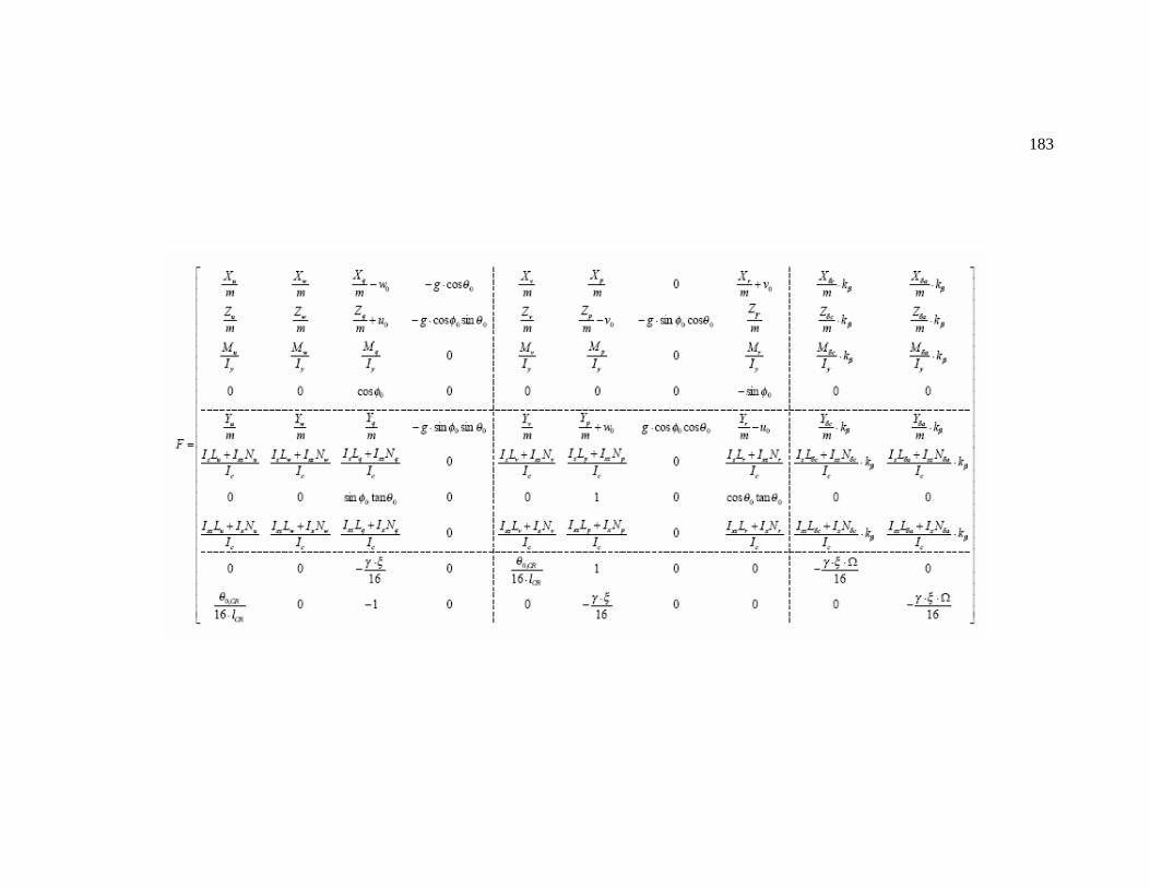
183
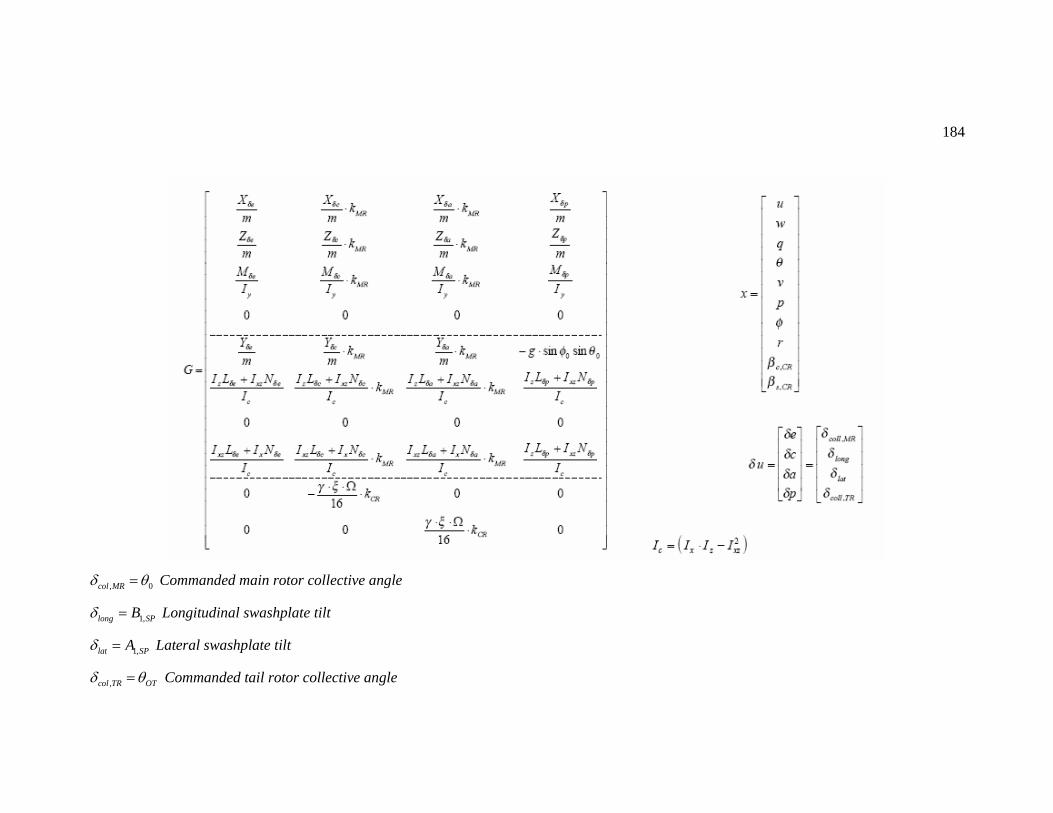
184
, 0col MRδ θ= Commanded main rotor collective angle
1,long SPBδ = Longitudinal swashplate tilt
1,lat SPAδ = Lateral swashplate tilt
,col TR OTδ θ= Commanded tail rotor collective angle

APPENDIX B
PITCH MECHANISM OF STABILIZER AND MAIN ROTOR BLADES
B1 Blade Pitch due to Collective Input
1 11 1
1 1b col
c z K zb e
θ ∆= = ∆
Swash plate
Pitch of Main Rotor
z∆
1c1b
1e
1d
1bθ

186
B2 Blade Pitch due to Cyclic Input
2 22
2 2b SP MR SP
c r Ke b
θ θ θ= =
swθ
2bθ
2b
2c
2e
Swash plate
Pitch of Main Rotor

187
B3 Pitch Angle of Stabilizer Bar
4 4
4 4sb SP CR SP
r l Ke m
θ θ θ= =
Swash plate
sbθ
4l
4r
4m
4e
swθ
Pitch of stabilizer
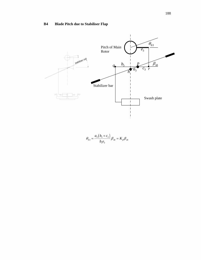
188
B4 Blade Pitch due to Stabiliser Flap
( )3 3 33
3 3b sb sb
a b cK
b e βθ β β+
= =
Stabilizer bar
Swash plate
Pitch of Main Rotor
sbβ
3bθ
3a3b
3c
3e
h
pqr
stabiliser rod
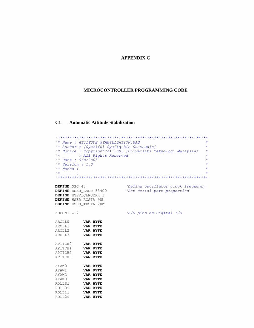
APPENDIX C
MICROCONTROLLER PROGRAMMING CODE
C1 Automatic Attitude Stabilization
'**************************************************************** '* Name : ATTITUDE STABILISATION.BAS * '* Author : [Syariful Syafiq Bin Shamsudin] * '* Notice : Copyright(c) 2005 [Universiti Teknologi Malaysia] * '* : All Rights Reserved * '* Date : 9/8/2005 * '* Version : 1.0 * '* Notes : * '* : * '**************************************************************** DEFINE OSC 40 ‘Define oscillator clock frequency DEFINE HSER_BAUD 38400 ‘Set serial port properties DEFINE HSER_CLROERR 1 DEFINE HSER_RCSTA 90h DEFINE HSER_TXSTA 20h ADCON1 = 7 ‘A/D pins as Digital I/O AROLL0 VAR BYTE AROLL1 VAR BYTE AROLL2 VAR BYTE AROLL3 VAR BYTE APITCH0 VAR BYTE APITCH1 VAR BYTE APITCH2 VAR BYTE APITCH3 VAR BYTE AYAW0 VAR BYTE AYAW1 VAR BYTE AYAW2 VAR BYTE AYAW3 VAR BYTE ROLLSi VAR BYTE ROLL0i VAR BYTE ROLL1i VAR BYTE ROLL2i VAR BYTE

190
PITCHSi VAR BYTE PITCH0i VAR BYTE PITCH1i VAR BYTE YAWSi VAR BYTE YAW0i VAR BYTE YAW1i VAR BYTE YAW2i VAR BYTE ROLLS VAR BYTE ROLL0 VAR BYTE ROLL1 VAR BYTE ROLL2 VAR BYTE PITCHS VAR BYTE PITCH0 VAR BYTE PITCH1 VAR BYTE YAWS VAR BYTE YAW0 VAR BYTE YAW1 VAR BYTE YAW2 VAR BYTE ROLLDi VAR BYTE PITCHDi VAR BYTE YAWDi VAR BYTE ROLLD VAR BYTE PITCHD VAR BYTE YAWD VAR BYTE ROLLDs VAR BYTE PITCHDs VAR BYTE YAWDs VAR BYTE B0 VAR WORD B1 VAR WORD B2 VAR WORD B3 VAR WORD B4 VAR WORD B5 VAR WORD PULREC VAR WORD portd = 0 B1 = 1501 'yaw B2 = 1460 'roll B3 = 1550 'pitch B4 = 100 TRISB = 255 'set pin B to input or (TRISB = % 11111111) TRISD = 0 'set pin D to output 'Change AHRS mode from raw data to Euler angle mode '**************************************************************** PAUSE 1000 HSEROUT ["!00001",13] PAUSE 1000 '**************************************************************** servoINIT:

191
B4 = (B4 - 1) portd.0 = 1 PAUSEUS B2 portd.0 = 0 portd.1 = 1 PAUSEUS B3 portd.1 = 0 portd.3 = 1 PAUSEUS B1 portd.3 = 0 PAUSE 20 IF B4 = 0 THEN GOTO servoINITEND ELSE GOTO servoINIT ENDIF servoINITEND: STARTA: IF portb.7 = 1 THEN GOTO MANUAL ELSE GOTO INITIATE ENDIF MANUAL: PORTD = PORTB GOTO STARTA INITIATE: '################################################################### '################################################################### '################################################################### HSERIN [WAIT("E:"),STR AROLL0\1,STR AROLL1\1,STR AROLL2\1,STR AROLL3\1,_WAIT(","),STR APITCH0\1,STR APITCH1\1,STR APITCH2\1,STR APITCH3\1,_WAIT(","),STR AYAW0\1,STR AYAW1\1,STR AYAW2\1,STR AYAW3\1] '################################################################### '################################################################### '################################################################### ROLLi: IF (AROLL0 = 45) THEN GOTO RNEGATIFi ELSE GOTO RPOSITIVEi ENDIF '=========================================== '=========================================== '=========================================== RNEGATIFi: IF (AROLL2 = 46) THEN GOTO RNEGATIF_1i ELSE GOTO RNEGATIF_23i

192
ENDIF RNEGATIF_1i: ROLLSi = 1 ROLL0i = 0 ROLL1i = 0 ROLL2i = (AROLL1 - 48) GOTO PITCHi RNEGATIF_23i: IF (AROLL3 = 46) THEN GOTO RNEGATIF_2i ELSE GOTO RNEGATIF_3i ENDIF RNEGATIF_2i: ROLLSi = 1 ROLL0i = 0 ROLL1i = (AROLL1 - 48) ROLL2i = (AROLL2 - 48) GOTO PITCHi RNEGATIF_3i: ROLLSi = 1 ROLL0i = (AROLL1 - 48) ROLL1i = (AROLL2 - 48) ROLL2i = (AROLL3 - 48) GOTO PITCHi '=========================================== '=========================================== '=========================================== RPOSITIVEi: IF (AROLL1 = 46) THEN GOTO RPOSITIVE_1i ELSE GOTO RPOSITIVE_23i ENDIF '=========================================== RPOSITIVE_1i: ROLLSi = 0 ROLL0i = 0 ROLL1i = 0 ROLL2i = (AROLL0 - 48) GOTO PITCHi RPOSITIVE_23i: IF (AROLL2 = 46) THEN GOTO RPOSITIVE_2i ELSE GOTO RPOSITIVE_3i ENDIF RPOSITIVE_2i: ROLLSi = 0 ROLL0i = 0

193
ROLL1i = (AROLL0 - 48) ROLL2i = (AROLL1 - 48) GOTO PITCHi RPOSITIVE_3i: ROLLSi = 0 ROLL0i = (AROLL0 - 48) ROLL1i = (AROLL1 - 48) ROLL2i = (AROLL2 - 48) GOTO PITCHi '################################################################### '################################################################### '################################################################### PITCHi: IF (APITCH0 = 45) THEN GOTO PNEGATIFi ELSE GOTO PPOSITIVEi ENDIF '=========================================== '=========================================== '=========================================== PNEGATIFi: IF (APITCH2 = 46) THEN GOTO PNEGATIF_1i ELSE GOTO PNEGATIF_2i ENDIF PNEGATIF_1i: PITCHSi = 1 PITCH0i = 0 PITCH1i = (APITCH1 - 48) GOTO YAWi PNEGATIF_2i: PITCHSi = 1 PITCH0i = (APITCH1 - 48) PITCH1i = (APITCH2 - 48) GOTO YAWi '=========================================== '=========================================== '=========================================== PPOSITIVEi: IF (APITCH1 = 46) THEN GOTO PPOSITIVE_1i ELSE GOTO PPOSITIVE_2i ENDIF '=========================================== PPOSITIVE_1i: PITCHSi = 0 PITCH0i = 0 PITCH1i = (APITCH0 - 48)
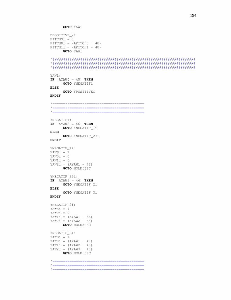
194
GOTO YAWi PPOSITIVE_2i: PITCHSi = 0 PITCH0i = (APITCH0 - 48) PITCH1i = (APITCH1 - 48) GOTO YAWi '################################################################### '################################################################### '################################################################### YAWi: IF (AYAW0 = 45) THEN GOTO YNEGATIFi ELSE GOTO YPOSITIVEi ENDIF '=========================================== '=========================================== '=========================================== YNEGATIFi: IF (AYAW2 = 46) THEN GOTO YNEGATIF_1i ELSE GOTO YNEGATIF_23i ENDIF YNEGATIF_1i: YAWSi = 1 YAW0i = 0 YAW1i = 0 YAW2i = (AYAW1 - 48) GOTO HOLD5SEC YNEGATIF_23i: IF (AYAW3 = 46) THEN GOTO YNEGATIF_2i ELSE GOTO YNEGATIF_3i ENDIF YNEGATIF_2i: YAWSi = 1 YAW0i = 0 YAW1i = (AYAW1 - 48) YAW2i = (AYAW2 - 48) GOTO HOLD5SEC YNEGATIF_3i: YAWSi = 1 YAW0i = (AYAW1 - 48) YAW1i = (AYAW2 - 48) YAW2i = (AYAW3 - 48) GOTO HOLD5SEC '=========================================== '=========================================== '===========================================

195
YPOSITIVEi: IF (AYAW1 = 46) THEN GOTO YPOSITIVE_1i ELSE GOTO YPOSITIVE_23i ENDIF '=========================================== YPOSITIVE_1i: YAWSi = 0 YAW0i = 0 YAW1i = 0 YAW2i = (AYAW0 - 48) GOTO HOLD5SEC YPOSITIVE_23i: IF (AYAW2 = 46) THEN GOTO YPOSITIVE_2i ELSE GOTO YPOSITIVE_3i ENDIF YPOSITIVE_2i: YAWSi = 0 YAW0i = 0 YAW1i = (AYAW0 - 48) YAW2i = (AYAW1 - 48) GOTO HOLD5SEC YPOSITIVE_3i: YAWSi = 0 YAW0i = (AYAW0 - 48) YAW1i = (AYAW1 - 48) YAW2i = (AYAW2 - 48) GOTO HOLD5SEC '################################################################### '################################################################### '################################################################### HOLD5SEC: ROLLDi = (ROLL0i * 100) + (ROLL1i * 10) + (ROLL2i) PITCHDi = (PITCH0i * 10) + (PITCH1i) YAWDi = (YAW0i * 100) + (YAW1i * 10) + (YAW2i) '################################################################### '################################################################### '################################################################### '################################################################### START: HSERIN [WAIT("E:"),STR AROLL0\1,STR AROLL1\1,STR AROLL2\1,STR AROLL3\1,_ WAIT(","),STR APITCH0\1,STR APITCH1\1,STR APITCH2\1,STR APITCH3\1,_ WAIT(","),STR AYAW0\1,STR AYAW1\1,STR AYAW2\1,STR AYAW3\1] '################################################################### '################################################################### '###################################################################
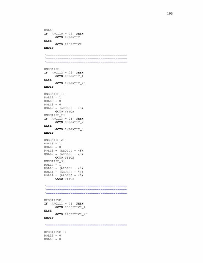
196
ROLL: IF (AROLL0 = 45) THEN GOTO RNEGATIF ELSE GOTO RPOSITIVE ENDIF '=========================================== '=========================================== '=========================================== RNEGATIF: IF (AROLL2 = 46) THEN GOTO RNEGATIF_1 ELSE GOTO RNEGATIF_23 ENDIF RNEGATIF_1: ROLLS = 1 ROLL0 = 0 ROLL1 = 0 ROLL2 = (AROLL1 - 48) GOTO PITCH RNEGATIF_23: IF (AROLL3 = 46) THEN GOTO RNEGATIF_2 ELSE GOTO RNEGATIF_3 ENDIF RNEGATIF_2: ROLLS = 1 ROLL0 = 0 ROLL1 = (AROLL1 - 48) ROLL2 = (AROLL2 - 48) GOTO PITCH RNEGATIF_3: ROLLS = 1 ROLL0 = (AROLL1 - 48) ROLL1 = (AROLL2 - 48) ROLL2 = (AROLL3 - 48) GOTO PITCH '=========================================== '=========================================== '=========================================== RPOSITIVE: IF (AROLL1 = 46) THEN GOTO RPOSITIVE_1 ELSE GOTO RPOSITIVE_23 ENDIF '=========================================== RPOSITIVE_1: ROLLS = 0 ROLL0 = 0

197
ROLL1 = 0 ROLL2 = (AROLL0 - 48) GOTO PITCH RPOSITIVE_23: IF (AROLL2 = 46) THEN GOTO RPOSITIVE_2 ELSE GOTO RPOSITIVE_3 ENDIF RPOSITIVE_2: ROLLS = 0 ROLL0 = 0 ROLL1 = (AROLL0 - 48) ROLL2 = (AROLL1 - 48) GOTO PITCH RPOSITIVE_3: ROLLS = 0 ROLL0 = (AROLL0 - 48) ROLL1 = (AROLL1 - 48) ROLL2 = (AROLL2 - 48) GOTO PITCH '################################################################### '################################################################### '################################################################### PITCH: IF (APITCH0 = 45) THEN GOTO PNEGATIF ELSE GOTO PPOSITIVE ENDIF '=========================================== '=========================================== '=========================================== PNEGATIF: IF (APITCH2 = 46) THEN GOTO PNEGATIF_1 ELSE GOTO PNEGATIF_2 ENDIF PNEGATIF_1: PITCHS = 1 PITCH0 = 0 PITCH1 = (APITCH1 - 48) GOTO YAW PNEGATIF_2: PITCHS = 1 PITCH0 = (APITCH1 - 48) PITCH1 = (APITCH2 - 48) GOTO YAW '=========================================== '===========================================

198
'=========================================== PPOSITIVE: IF (APITCH1 = 46) THEN GOTO PPOSITIVE_1 ELSE GOTO PPOSITIVE_2 ENDIF '=========================================== PPOSITIVE_1: PITCHS = 0 PITCH0 = 0 PITCH1 = (APITCH0 - 48) GOTO YAW PPOSITIVE_2: PITCHS = 0 PITCH0 = (APITCH0 - 48) PITCH1 = (APITCH1 - 48) GOTO YAW '################################################################### '################################################################### '################################################################### YAW: IF (AYAW0 = 45) THEN GOTO YNEGATIF ELSE GOTO YPOSITIVE ENDIF '=========================================== '=========================================== '=========================================== YNEGATIF: IF (AYAW2 = 46) THEN GOTO YNEGATIF_1 ELSE GOTO YNEGATIF_23 ENDIF YNEGATIF_1: YAWS = 1 YAW0 = 0 YAW1 = 0 YAW2 = (AYAW1 - 48) GOTO SROLL YNEGATIF_23: IF (AYAW3 = 46) THEN GOTO YNEGATIF_2 ELSE GOTO YNEGATIF_3 ENDIF YNEGATIF_2: YAWS = 1

199
YAW0 = 0 YAW1 = (AYAW1 - 48) YAW2 = (AYAW2 - 48) GOTO SROLL YNEGATIF_3: YAWS = 1 YAW0 = (AYAW1 - 48) YAW1 = (AYAW2 - 48) YAW2 = (AYAW3 - 48) GOTO SROLL '=========================================== '=========================================== '=========================================== YPOSITIVE: IF (AYAW1 = 46) THEN GOTO YPOSITIVE_1 ELSE GOTO YPOSITIVE_23 ENDIF '=========================================== YPOSITIVE_1: YAWS = 0 YAW0 = 0 YAW1 = 0 YAW2 = (AYAW0 - 48) GOTO SROLL YPOSITIVE_23: IF (AYAW2 = 46) THEN GOTO YPOSITIVE_2 ELSE GOTO YPOSITIVE_3 ENDIF YPOSITIVE_2: YAWS = 0 YAW0 = 0 YAW1 = (AYAW0 - 48) YAW2 = (AYAW1 - 48) GOTO SROLL YPOSITIVE_3: YAWS = 0 YAW0 = (AYAW0 - 48) YAW1 = (AYAW1 - 48) YAW2 = (AYAW2 - 48) GOTO SROLL '################################################################### '################################################################### '################################################################### SROLL: ROLLD = (ROLL0 * 100) + (ROLL1 * 10) + (ROLL2) PITCHD = (PITCH0 * 10) + (PITCH1) YAWD = (YAW0 * 100) + (YAW1 * 10) + (YAW2)

200
IF (ROLLDi > ROLLD) THEN ROLLDs = (ROLLDi - ROLLD) ELSE ROLLDs = (ROLLD - ROLLDi) ENDIF IF (PITCHDi > PITCHD) THEN PITCHDs = (PITCHDi - PITCHD) ELSE PITCHDs = (PITCHD - PITCHDi) ENDIF IF (YAWDi > YAWD) THEN YAWDs = (YAWDi - YAWD) ELSE YAWDs = (YAWD - YAWDi) ENDIF '================================================= IF (ROLLSi = 1) THEN GOTO SROLLN ELSE GOTO SROLLP ENDIF '================================================= SROLLN: IF (ROLLS = 1) THEN GOTO SROLLNN ELSE GOTO rollleft ENDIF SROLLNN: IF (ROLLD > ROLLDi) THEN GOTO rollright ELSE GOTO rollleft ENDIF '================================================= SROLLP: IF (ROLLS = 1) THEN GOTO rollright ELSE GOTO SROLLPP ENDIF SROLLPP: IF (ROLLD > ROLLDi) THEN GOTO rollleft ELSE GOTO rollright ENDIF '================================================= rollright:

201
B2 = B2 + ROLLDs IF b2 > 1860 THEN rollrightmax GOSUB servoroll GOTO SPITCH rollleft: B2 = B2 - ROLLDs IF b2 < 1140 THEN rollleftmin GOSUB servoroll GOTO SPITCH rollrightmax: B2 = 1860 GOSUB servoroll GOTO SPITCH rollleftmin: B2 = 1140 GOSUB servoroll GOTO SPITCH '################################################################### '################################################################### '################################################################### SPITCH: IF (PITCHSi = 1) THEN GOTO SPITCHN ELSE GOTO SPITCHP ENDIF '================================================= SPITCHN: IF (PITCHS = 1) THEN GOTO SPITCHNN ELSE GOTO PITCHleft ENDIF SPITCHNN: IF (PITCHD > PITCHDi) THEN GOTO PITCHright ELSE GOTO PITCHleft ENDIF '================================================= SPITCHP: IF (PITCHS = 1) THEN GOTO PITCHright ELSE GOTO SPITCHPP ENDIF SPITCHPP: IF (PITCHD > PITCHDi) THEN GOTO PITCHleft ELSE

202
GOTO PITCHright ENDIF '================================================= PITCHright: 'move to aft B3 = B3 + PITCHDs IF B3 > 1820 THEN PITCHrightmax GOSUB servopitch GOTO SYAW PITCHleft: ' move to front B3 = B3 - PITCHDs IF B3 < 1270 THEN PITCHleftmin GOSUB servopitch GOTO SYAW PITCHrightmax: B3 = 1820 GOSUB servopitch GOTO SYAW PITCHleftmin: B3 = 1270 GOSUB servopitch GOTO SYAW '################################################################### '################################################################### '################################################################### SYAW: IF (YAWSi = 1) THEN GOTO SYAWN ELSE GOTO SYAWP ENDIF '================================================= SYAWN: IF (YAWS = 1) THEN GOTO SYAWNN ELSE GOTO YAWleft ENDIF SYAWNN: IF (YAWD > YAWDi) THEN GOTO YAWright ELSE GOTO YAWleft ENDIF '================================================= SYAWP: IF (YAWS = 1) THEN GOTO YAWright ELSE GOTO SYAWPP ENDIF

203
SYAWPP: IF (YAWD > YAWDi) THEN GOTO YAWleft ELSE GOTO YAWright ENDIF '================================================= YAWright: B1 = B1 + (YAWDs*YAWDs) IF B1 > 1900 THEN YAWrightmax GOSUB servoyaw GOTO STARTC YAWleft: B1 = B1 - (YAWDs*YAWDs) IF B1 < 1110 THEN YAWleftmin GOSUB servoyaw GOTO STARTC YAWrightmax: B1 = 1900 GOSUB servoyaw GOTO STARTC YAWleftmin: B1 = 1110 GOSUB servoyaw GOTO STARTC STARTC: IF portb.7 = 1 THEN GOTO STARTA ELSE GOTO START ENDIF '################################################################### '################################################################### END servoroll: portd.0 = 1 PAUSEUS B2 portd.0 = 0 RETURN servopitch: portd.1 = 1 PAUSEUS B3 portd.1 = 0 RETURN servoyaw: portd.3 = 1 PAUSEUS B1 portd.3 = 0 RETURN

204
C2 Manual-Automatic Control Switching
'**************************************************************** '* Name : Manual-Automatic Control Switching.BAS * '* Author : [Syariful Syafiq bin Shamsudin] * '* Notice : Copyright(c) 2006 [Universiti Teknologi Malaysia] * '* : All Rights Reserved * '* Date : 1/17/2006 * '* Version : 1.0 * '* Notes : * '* : * '**************************************************************** DEFINE OSC 20 PULREC VAR WORD TRISA = 0 TRISB = 255 '**************************************************************** START: PULSIN PORTB.0,1,PULREC IF (PULREC < 750) THEN GOTO OFFPT ELSE GOTO ONPT ENDIF OFFPT: LOW PORTA.0 GOTO START ONPT: HIGH PORTA.0 GOTO START END

APPENDIX D
PIC18F2420/2520/4420/4520 MICROCONTROLLER PINOUT
DESCRIPTIONS

206
D1 PIC18F4420/4520 (40/44-PIN) Block Diagram (Microchip Technology
Inc, 2004)

207
D2 PIC18F4420/4520 PINOUT I/O DESCRIPTIONS (Microchip
Technology Inc, 2004)

208

209

210

APPENDIX E
LIST OF PUBLICATIONS
E1 Conference Papers
• Abas Ab. Wahab, Rosbi Mamat and Syariful Syafiq Shamsudin (2006).
The Development of Autopilot System for UTM Autonomous UAV
Helicopter Model 1st Regional Conference on Vehicle Engineering and
Technology (RIVET 2006). 3-5 July, Kuala Lumpur: Automotive,
Aeronautic & Marine Focus Group, RMC, UTM.
• Ab. Wahab, Rosbi Mamat and Syariful Syafiq Shamsudin (2006). Control
System Design For UTM Autonomous Helicopter Model In Hovering
Using Pole Placement Method. 1st Regional Conference on Vehicle
Engineering and Technology (RIVET 2006). 3-5 July. Kuala Lumpur:
Automotive, Aeronautic & Marine Focus Group, RMC, UTM.
• Abas Ab. Wahab, Rosbi Mamat and Syariful Syafiq Shamsudin (2004).
The Preliminary Study of System Identification Modeling of a Model
Scale Helicopter in Hovering, Malaysian Science and Technology
Congress (MSTC 2004. 5-7 October. Kuala Lumpur: COSTAM.