heliospheric tomography - ccmc: community · pdf fileheliospheric tomography b.v. jackson,...

CASS/UCSD CCMC 2010

Heliospheric TomographyB.V. Jackson,

and

P.P. Hick, A. Buffington, M.M. Bisi, J.M. Clover, S. HamiltonCenter for Astrophysics and Space Sciences, University of California at San Diego, LaJolla, CA, USA

Masayoshi

Heliospheric Tomography

http://smei.ucsd.edu/ http://ips.ucsd.edu/

andM. Tokumaru, K. Fujiki,Solar-Terrestrial Environment Laboratory, Nagoya University, Furo-cho, Chikusa-ku, Nagoya, Japan

andP.K. ManoharanRadio Astronomy Centre, National Centre for Radio Astrophysics, Tata Institute of Fundamental Research, Udhagamandalam (Ooty), 643 001, India

CASS/UCSD CCMC 2010


The Model: Heliospheric Tomography – (actually a fit to data)(Time-dependent view from a single observer location)

The Data Sets:IPS (STELab, Ooty, EISCAT), SMEI(How the model validates different data sets)

New Projects:FR inversionIn-situ incorporation into the tomographyReal-time SMEI

Introduction:

CASS/UCSD CCMC 2010


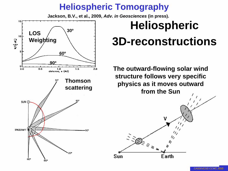
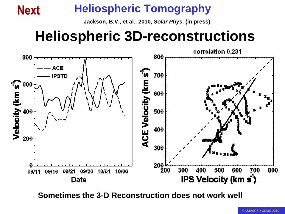
Heliospheric 3D-reconstructions

Thomson scattering

The outward-flowing solar wind structure follows very specific physics as it moves outward

from the Sun

LOS Weighting

30º

60º

90º

Jackson, B.V., et al., 2009, Adv. in Geosciences (in press).

CASS/UCSD CCMC 2010


The “traceback

matrix”

(any model will work)

In the traceback

matrix the location of the upper level data point (starred) is an interpolation in x of Δx2 and the unit x distance –

Δx3 distance or (1 –

Δx3). Similarly, the value of Δt

at the starred point is interpolated by the same spatial distance. Each 3D traceback

matrix contains a regular grid of values ΣΔx, ΣΔy, ΣΔt, ΣΔv, and ΣΔm

that locates the origin of each point in the grid at each time and its change in velocity and density from the heliospheric

model.

The UCSD 3D-reconstruction programJackson, B.V., et al., 2009, Adv. in Geosciences (in press).

CASS/UCSD CCMC 2010


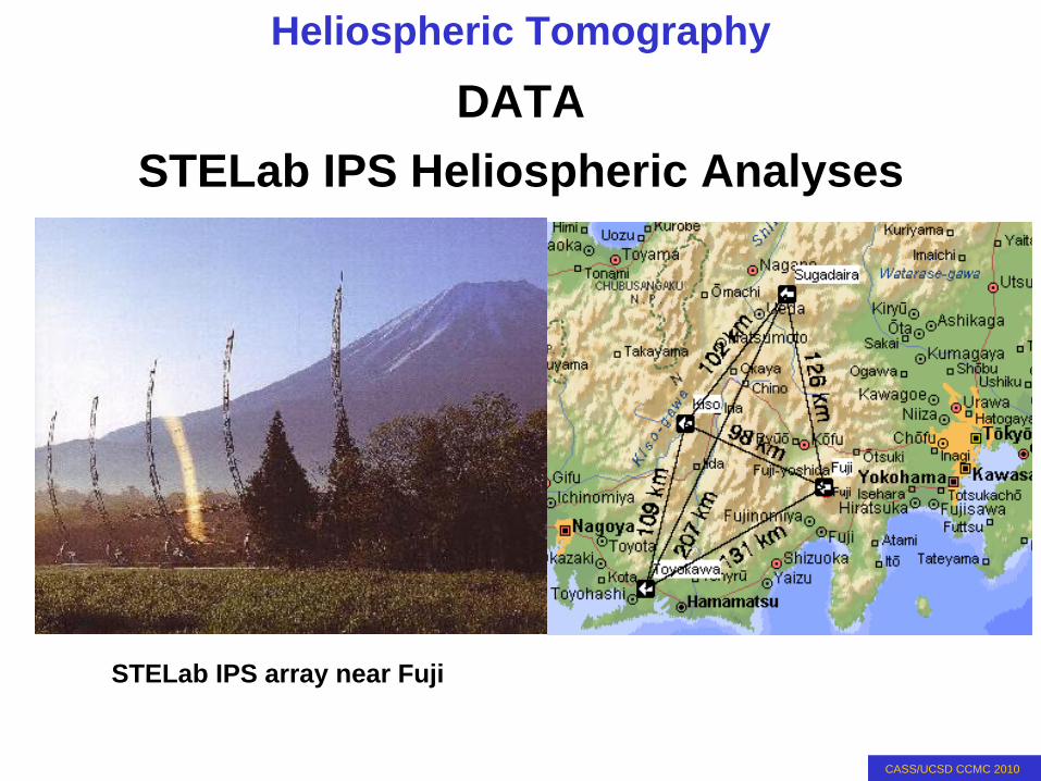
STELab IPS Heliospheric Analyses

STELab IPS array near Fuji

DATA

CASS/UCSD CCMC 2010


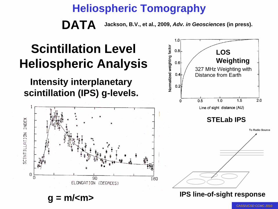
Scintillation Level Heliospheric Analysis

g = m/<m>

Intensity interplanetary scintillation (IPS) g-levels.

LOS Weighting

STELab IPS

IPS line-of-sight response

DATA Jackson, B.V., et al., 2009, Adv. in Geosciences (in press).

CASS/UCSD CCMC 2010


Web Analysis Runs Automatically Using Linux on a P.C.

Real-time tomographic

analysis of the solar wind on April 29-30, 2004 showing a halo CME response in the interplanetary medium.

Velocity model time-series G-level sky map

http://ips.ucsd.edu/

UCSD time-dependent IPS WEB model

CASS/UCSD CCMC 2010


Simultaneous images from the three SMEI cameras.

SMEIC1

C2

C3

Sun

Sun|V

1 gigabyte/day; now ~3 terabytesLaunch 6 January 2003

DATA Jackson, B.V., et al., 2006, J. Geophys. Res., 111, A4, A04S91

CASS/UCSD CCMC 2010


Frame Composite for Aitoff MapBlue = Cam3; Green = Cam2; Red = Cam1

D290; 17 October 2003

DATA

CASS/UCSD CCMC 2010


Brightness fall-off with distance

0 30 60 90 120 150 180Elongation degrees

Zodiacal light (ecliptic)Zodiacal light (high latitude)StarsCMEs (HELIOS extrapolated)Ambient (density 10/cc)

Inte

nsity

rela

tive

to S

olar

10-15

10-14

10-13

10-12

10-11

10-10

10-9

DATA Jackson, B.V., et al., 2009, Solar Phys. (in press).

CASS/UCSD CCMC 2010


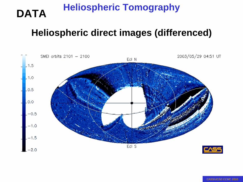
Heliospheric direct images (differenced)

DATA

CASS/UCSD CCMC 2010


SMEI Brightness with a long-term (~30 day) base removed. (1 S10 = 0.46 ± 0.02 ADU)

27-28 May 2003 CME events brightness time seriesfor select sky sidereal locations

DATA

Jackson, B.V., et al., 2008, J. Geophys Res., 113, A00A15, doi:10.1029/2008JA013224

CASS/UCSD CCMC 2010


Heliospheric 3-D Reconstruction

Line of sight “crossed”

components on a reference surface. Projections on the reference surface are shown. These weighted components are inverted to provide the time-dependent tomographic

reconstruction.

Jackson, B.V., et al., 2009, Adv. in Geosciences (in press).

CASS/UCSD CCMC 2010


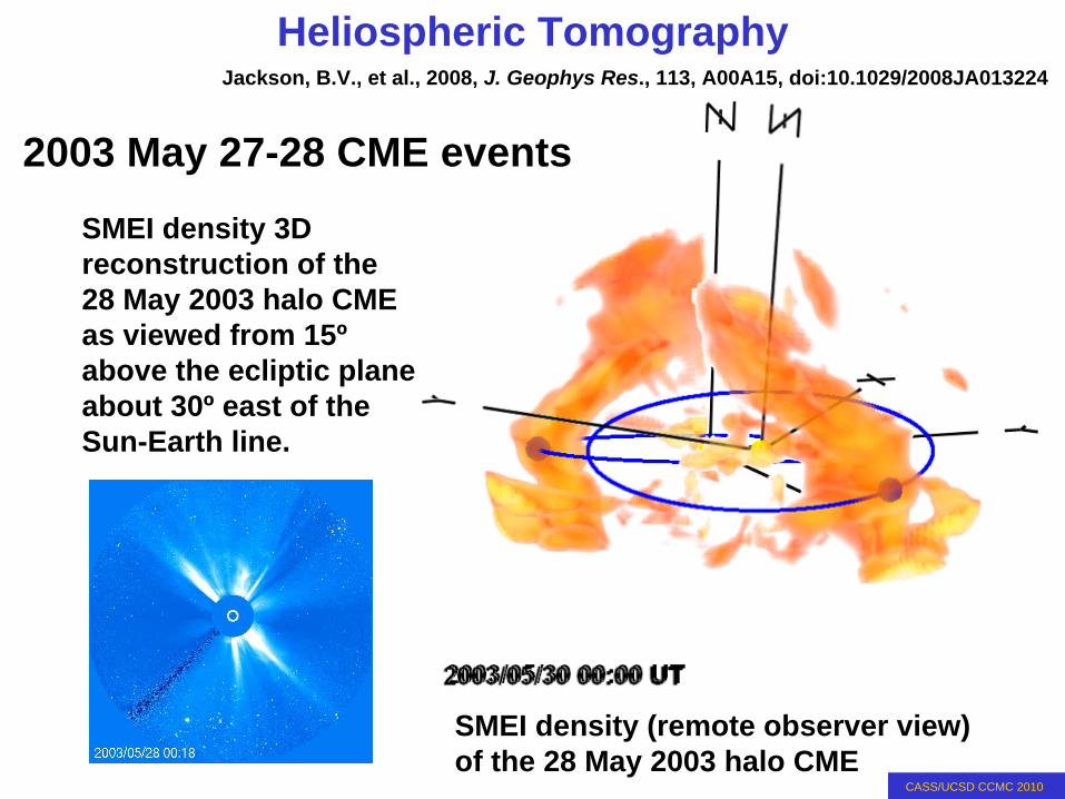
SMEI density (remote observer view) of the 28 May 2003 halo CME

2003 May 27-28 CME events

SMEI density 3D reconstruction of the 28 May 2003 halo CME as viewed from 15º above the ecliptic plane about 30º east of the Sun-Earth line.


CASS/UCSD CCMC 2010


2003 May 27-28 CME eventsCME masses


CASS/UCSD CCMC 2010


IPS Velocity and SMEI proton density reconstruction of the 27-28 May 2003 halo CME sequence. Reconstructed and Wind in-situ densities are compared with over one Carrington rotation.

27-28 May 2003 CME event periodJackson, B.V., et al., 2008, J. Geophys Res., 113, A00A15, doi:10.1029/2008JA013224

CASS/UCSD CCMC 2010


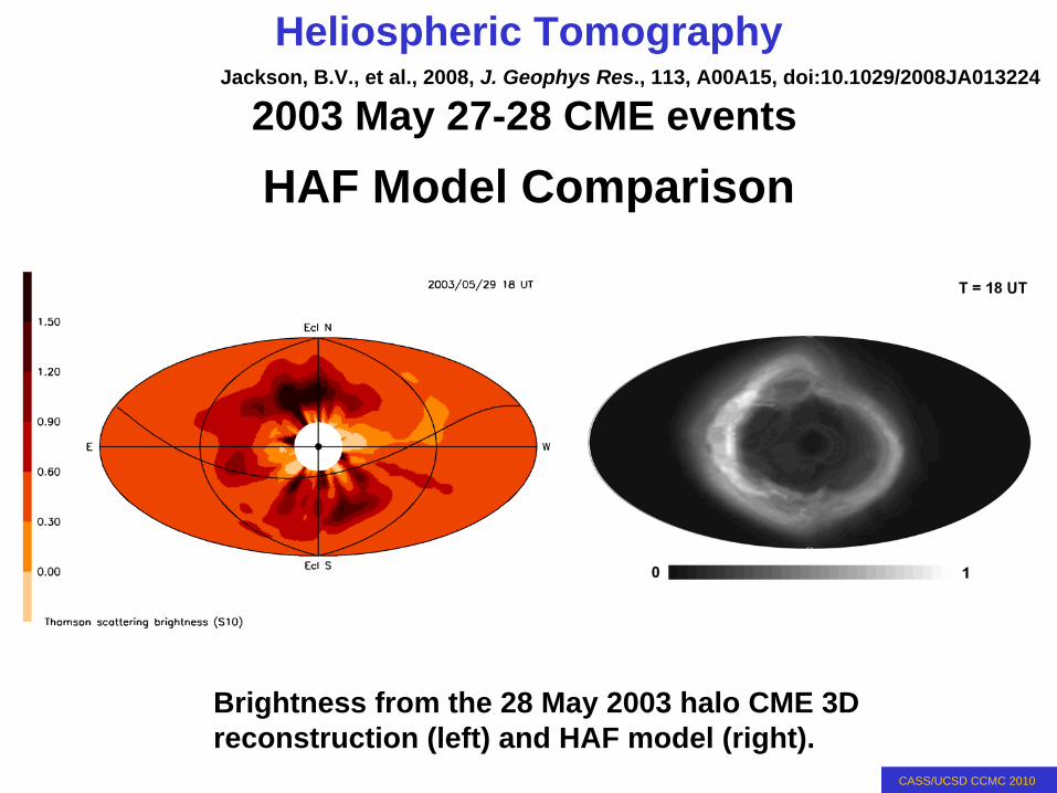
HAF Model Comparison2003 May 27-28 CME events

Brightness from the 28 May 2003 halo CME 3D reconstruction (left) and HAF model (right).


CASS/UCSD CCMC 2010

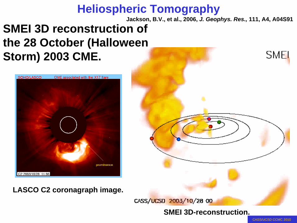
Heliospheric TomographySMEI 3D reconstruction of the 28 October (Halloween Storm) 2003 CME.

SMEI 3D-reconstruction.

LASCO C2 coronagraph image.

Jackson, B.V., et al., 2006, J. Geophys. Res., 111, A4, A04S91

CASS/UCSD CCMC 2010

Heliospheric TomographyRecent higher-resolution SMEI PC 3D reconstructions show

the CME sheath region as well as the central dense core

28 October 2003 CME “Halloween storm” ICME

Ecliptic cuts

shock

CASS/UCSD CCMC 2010


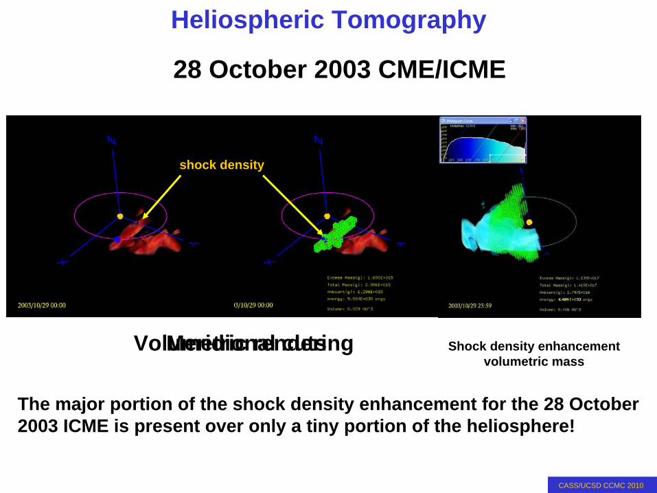
Meridional cutsVolumetric rendering

The major portion of the shock density enhancement for the 28 October 2003 ICME is present over only a tiny portion of the heliosphere!

28 October 2003 CME/ICME

Shock density enhancement volumetric mass

shock density

CASS/UCSD CCMC 2010


The 20 January 2005 flare/ CME is associated with a very energetic (and prompt) SEP.

Ulysses

.

SMEI

LASCO C2 coronagraph difference image.

20 January 2005 CME shock

Ulysses

SMEI Hammer-Aitoff image of the whole sky

CASS/UCSD CCMC 2010

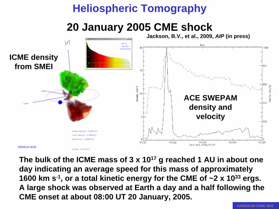
Heliospheric Tomography20 January 2005 CME shock

ICME density from SMEI

The bulk of the ICME mass of 3 x 1017 g reached 1 AU in about one day indicating an average speed for this mass of approximately 1600 km s-1, or a total kinetic energy for the CME of ~2 x 1033 ergs. A large shock was observed at Earth a day and a half following the CME onset at about 08:00 UT 20 January, 2005.

ACE SWEPAM density and

velocity

Jackson, B.V., et al., 2009, AIP (in press)

CASS/UCSD CCMC 2010

Heliospheric Tomography20 January 2005 CME shock

Meridional cutEcliptic cut

shock density

shock density

From volumetric data determine mass flow past the spacecraft by measuring the density along the radial from Sun to Earth. SMEI = 4.7×1013cm-2

From in situ data determine mass flow past the spacecraft by measuring the flux of material that has passed the spacecraft over time.

In-situ shock

Wind SWE = 4.54×1013, SOHO CELIAS = 6.55×1013, ACE SWEPAM L0 = 2.57×1013

Jackson, B.V., et al., 2009, AIP (in press)

CASS/UCSD CCMC 2010


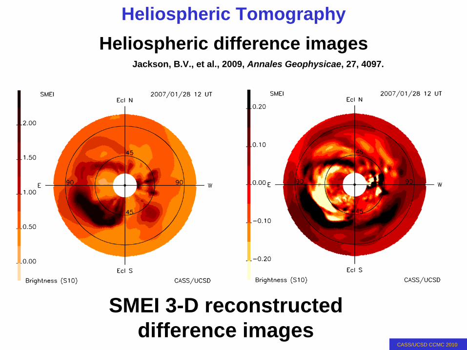
SMEI 3-D reconstructed difference images

Heliospheric difference imagesJackson, B.V., et al., 2009, Annales Geophysicae, 27, 4097.

CASS/UCSD CCMC 2010

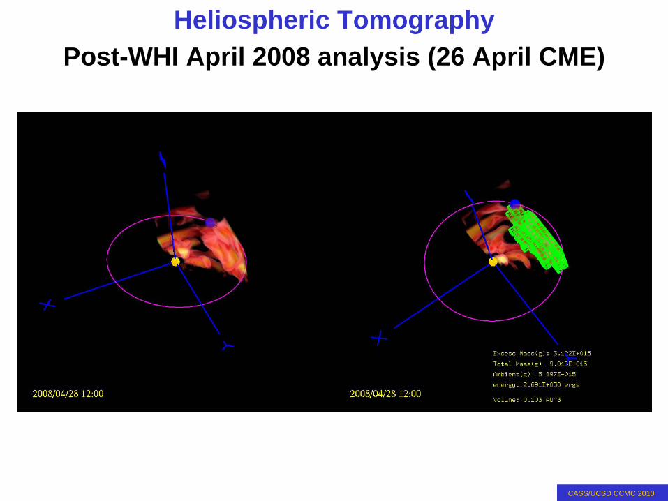
Heliospheric TomographyPost-WHI April 2008 analysis (26 April CME)

CME CME

East

West

CASS/UCSD CCMC 2010


The outward-flowing solar wind structure follows very specific physics as it moves outward from the Sun

CIR

CME

CME

Post-WHI April 2008 analysis (26 April CME)

CASS/UCSD CCMC 2010

Heliospheric TomographyPost-WHI April 2008 analysis (26 April CME)

CASS/UCSD CCMC 2010


SMEI data analysis

Line of sight crossing error example- the WHI period

CASS/UCSD CCMC 2010

Heliospheric TomographyOoty Density 3-D Reconstruction

The left movie shows an ecliptic cut through the 3D Ooty IPS density reconstruction and the right movie show a meridional cut (from East of the Sun-Earth line) of the same; both

with the Earth on the right-hand side and it’s orbit shown in each case

Other

The left shows an ecliptic cut through the 3D Ooty IPS density reconstruction and the right shows a meridional cut (from East of the Sun-Earth line) of the same; both with the Earth on the right-hand side and it’s orbit are shown.

Bisi, M.M., et al., 2009, Annales Geophysicae, 27, 4479.4-7 November 2004

CASS/UCSD CCMC 2010


The left shows an ecliptic cut through the 3D Ooty IPS speed reconstruction and the right shows a meridional cut (from East of the Sun-Earth line) of the same; both with the Earth on the right-hand side and it’s orbit are shown.

Ooty Velocity 3-D ReconstructionOther

Bisi, M.M., et al., 2009, Annales Geophysicae, 27, 4479.4-7 November 2004

CASS/UCSD CCMC 2010

Heliospheric TomographyOoty 3-D Density and Velocity ReconstructionOther Bisi, M.M., et al., 2009, Annales Geophysicae, 27, 4479.

CASS/UCSD CCMC 2010


It now becomes more important to be absolutely certain of the higher-frequency velocity LOS weighting.

EISCAT ResultOther

Bisi, M.M., et al., 2010, Solar Phys., (submitted)

Bisi, M.M., et al., 2010, Solar Phys. (submitted).

CASS/UCSD CCMC 2010

Heliospheric Tomography•Bisi, M.M., B.V. Jackson, A. Buffington, J.M. Clover, P.P. Hick, and M. Tokumaru, 2009, ‘Low-Resolution STELab IPS 3D Reconstructions of the Whole Heliosphere Interval and Comparison with in-Ecliptic Solar Wind Measurements from STEREO and Wind Instrumentation’, Solar Phys. - STEREO Science Results at Solar Minimum Topical Issue, 256, 201-217, doi:10.1007/s11207-009-9350-9.•Bisi, M.M., Jackson, B.V., Clover, J.M., Manoharan, P.K., Tokumaru, M., Hick, P.P., and. Buffington, A., 2009, ‘3D reconstructions of the early- November 2004 CDAW geomagnetic storms: analysis of Ooty IPS speed and density data’, Annales Geophysicae, 27, 4479.•Bisi, M.M., Jackson, B.V., Clover, J.M., Tokumaru, M., and Fujiki, K., 2009, ‘Large-Scale Heliospheric Structure during Solar-Minimum Conditions using a 3D Time-Dependent Reconstruction Solar-Wind Model and STELab IPS Observations’, in-press, American Institute of Physics (Solar Wind 12 Proceedings).•Bisi, M.M., Jackson, B.V., Clover, J.M., Hick, P.P., and Buffington, A., 2009, ‘3D Reconstructions of the Whole Heliosphere Interval and Comparison with in-Ecliptic Solar Wind Measurements from STEREO, ACE, and Wind Instrumentation: a Brief Summary’, XXVIIth IAU General Assembly, August 2009, Highlights of Astronomy, 15, 119.•Bisi, M.M., Jackson, B.V., Breen, A.R., Dorrian, G.D., Fallows, R.A., Clover, J.M., and Hick, P.P., 2009, ‘Three-Dimensional (3-D) Reconstructions of EISCAT IPS Velocity Data in the Declining Phase of Solar Cycle 23’, Solar Phys. (submitted).•Bisi, M.M., Breen, A.R., Jackson, B.V., Fallows, R.A., Walsh, A.P., Mikic, Z., Riley, P., Owen, C.J., Gonzalez-Esparza, A., Aguilar-Rodriguez, E., Morgan, H., Jensen, E.A., Wood, A.G., Tokumaru, M., Manoharan, P.K., Chashei, I.V., Giunta, A.S., Linker, J.A., Shishov, V.I., Tyul’bashev, S.A., Agalya, , G., Glubokova, S.K., Hamilton, M.S., Fujiki, K., Hick, P.P., Clover, J.M., Pinter, B., 2009, ‘From the Sun to the Earth: the 13 May 2005 Coronal Mass Ejection’, Solar Phys. (submitted).•Buffington, A., Bisi, M.M., Clover, J.M., Hick, P.P., Jackson, B.V., Kuchar, T.A., and Price, S.D., 2009, ‘Measurements of the Gegenschein brightness from the Solar Mass Ejection Imager (SMEI)’, Icarus, 203, 124, doi:10.1016/j.icarus.2009.04.007.•Jackson, B.V., Hick, P.P., Buffington, A., Bisi, M.M., and Clover, J.M., 2009, ‘SMEI direct, 3D-reconstruction sky maps and volumetric analyses, and their comparison with SOHO and STEREO observations’, Annales Geophysicae, 27, 4097.•Jackson, B.V., Hick, P.P., Buffington, A., Bisi, M.M., Clover, J.M., Tokumaru, M., and Fujiki, K., 2009, ‘3D Reconstruction of Density Enhancements Behind Interplanetary Shocks from Solar Mass Ejection Imager White-Light Observations’, American Institute of Physics (Solar Wind 12 Proceedings) (in press).•Jackson, B.V., Hick, P.P., Buffington, A., Bisi, M.M., Clover, J.M., and Tokumaru, M., 2009, ‘Solar Mass Ejection Imager (SMEI) and Interplanetary Scintillation (IPS) 3D-Reconstructions of the Inner Heliosphere’, Adv. in Geosciences (in press).•Jackson, B.V., Hick, P.P., Bisi, M.M., Clover, J.M., and Buffington, A., 2009, ‘Inclusion of in-situ Velocity Measurements in the UCSD Time-Dependent Tomography to Constrain and Better- Forecast Remote-Sensing Observations’, Solar Phys. (in-press).•Jackson, B.V., Buffington, A., Hick, P.P., Bisi, M.M., and Clover, J.M., 2009, A Heliospheric Imager for Deep Space: Lessons Learned from Helios, SMEI, and STEREO’, Solar Phys. (in press).•Jensen, E.A., Hick, P.P., Bisi, M.M., Jackson, B.V., Clover, J., and Mulligan, T.L., 2009, ‘Faraday Rotation Response to Coronal Mass Ejection Structure’, Solar Phys., (submitted).•Webb, D.F., Howard, T.A., Fry, C.D., Kuchar, T.A., Odstrcil, D., Jackson, B.V., Bisi, M.M., Harrison, R.A., Morrill, J.S., Howard, R.A., and Johnston, J.C., 2009, ‘Study of CME Propagation in the Inner Heliosphere: SMEI and STEREO HI Observations of the January 2007 Events’, Solar Phys.- STEREO Special Issue, 256, 239, doi:10.1007/s11207-009-9351-8.•Webb, D. F., Howard, T. A., Fry, C. D., Kuchar, T. A., Mizuno, D. R., Johnston, J. C., and Jackson, B. V., 2009, ‘Studying Geoeffective ICMEs between the Sun and Earth: Space Weather Implications of SMEI Observations’, Space Weather, 7, S05002, doi:10.1029/2008SW000409.

Last Year!!

CASS/UCSD CCMC 2010


UCSD Web Pageshttp://smei.ucsd.edu/

Next

CASS/UCSD CCMC 2010


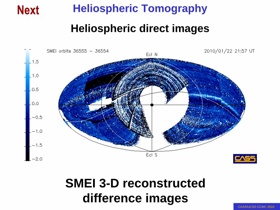
SMEI 3-D reconstructed difference images

Heliospheric direct imagesNext

CASS/UCSD CCMC 2010


New STELab IPS array at Toyokawa - photo February 17, 2007 (array now operates)

Current STELab IPS Heliospheric AnalysesNext

CASS/UCSD CCMC 2010


Background Field, 3D UCSD Density

Background Field, 3D UCSD Density, Mulligan “Can”

Faraday rotation tomographyNext

Jackson, B.V., et al., 2008, URAS Workshop

CASS/UCSD CCMC 2010


Heliospheric 3D-reconstructions

Sometimes the 3-D Reconstruction does not work well

NextJackson, B.V., et al., 2010, Solar Phys. (in press).

CASS/UCSD CCMC 2010


The Model: (not a model but a fit to data)•Allows a low-resolution 3-D reconstruction over time of most of the

heliosphere.

We’ve Learned some things:•How well our data collection system works.•The extent, shape, 3D mass, and energies of CMEs.•The latitude-longitude relationship and temporal evolution of

velocity structures globally in the heliosphere, and to CMEs.•In the SMEI highest-resolution tomography, the shock density

enhancements analyzed to date do not show a uniform shell-like extent. (?don’t know why).

The Future:•Better research with data sets that now provide a uniform answer.•Incorporation of the in-situ measurements into the tomography.•Incorporation of 3-D MHD into the tomography code.•FR inversion to obtain vector fields.

Summary:

heliospheric tomography - ccmc: community · pdf fileheliospheric tomography b.v. jackson,...

Documents