hendee - medical imaging physics (wiley,2002) - welcome to bioinnovel
TRANSCRIPT

C H A P T E R
19ULTRASOUND WAVES
OBJECTIVES 304
INTRODUCTION 304
HISTORY 304
WAVE MOTION 304
WAVE CHARACTERISTICS 305
ULTRASOUND INTENSITY 306
ULTRASOUND VELOCITY 307
ATTENUATION OF ULTRASOUND 308
REFLECTION 311
REFRACTION 313
ABSORPTION 314
SUMMARY 315
PROBLEMS 316
REFERENCES 316
Medical Imaging Physics, Fourth Edition, by William R. Hendee and E. Russell RitenourISBN: 0-471-38226-4 Copyright C© 2002 Wiley-Liss, Inc. 303

304 x ULTRASOUND WAVES
¥ OBJECTIVES
From studying this chapter, the reader should be able to:
r Explain the properties of ultrasound waves.r Describe the decibel notation for ultrasound intensity and pressure.r Delineate the ultrasound properties of velocity, attenuation, and absorption.r Depict the consequences of an impedance mismatch at the boundary between
two regions of tissue.r Explain ultrasound reflection, refraction and scattering.
¥ INTRODUCTION
Ultrasound is a mechanical disturbance that moves as a pressure wave through amedium. When the medium is a patient, the wavelike disturbance is the basis for useof ultrasound as a diagnostic tool. Appreciation of the characteristics of ultrasoundwaves and their behavior in various media is essential to understanding the use ofdiagnostic ultrasound in clinical medicine.1–6
In 1794, Spallanzi suggested correctly
that bats avoided obstacles during flight
by using sound signals beyond the
range of the human ear.
¥ HISTORY
In 1880, French physicists Pierre and Jacques Curie discovered the piezoelectriceffect.7 French physicist Paul Langevin attempted to develop piezoelectric materi-als as senders and receivers of high-frequency mechanical disturbances (ultrasoundwaves) through materials.8 His specific application was the use of ultrasound to de-tect submarines during World War I. This technique, sound navigation and ranging(SONAR), finally became practical during World War II. Industrial uses of ultra-sound began in 1928 with the suggestion of Soviet Physicist Sokolov that it couldbe used to detect hidden flaws in materials. Medical uses of ultrasound throughthe 1930s were confined to therapeutic applications such as cancer treatments andphysical therapy for various ailments. Diagnostic applications of ultrasound began inthe late 1940s through collaboration between physicians and engineers familiar withSONAR.9
¥ WAVE MOTION
A fluid medium is a collection of molecules that are in continuous random motion. Themolecules are represented as filled circles in the margin figure (Margin Figure 19-1).When no external force is applied to the medium, the molecules are distributedmore or less uniformly (A). When a force is applied to the medium (represented bymovement of the piston from left to right in B), the molecules are concentrated infront of the piston, resulting in an increased pressure at that location. The region ofincreased pressure is termed a zone of compression. Because of the forward motionimparted to the molecules by the piston, the region of increased pressure beginsto migrate away from the piston and through the medium. That is, a mechanicaldisturbance introduced into the medium travels through the medium in a directionaway from the source of the disturbance. In clinical applications of ultrasound, thepiston is replaced by an ultrasound transducer.
“Piezo” is Greek for pressure.
Piezoelectricity refers to the generation
of an electrical response to applied
pressure.
Pierre Curie used the piezoelectric
properties of quartz crystals to
construct a device to measure the small
changes in mass that accompany
radioactive decay. This work was done
in collaboration with his wife Marie in
her early studies of radioactivity.
The term “transducer” refers to any
device that converts energy from one
form to another (mechanical to
electrical, electrical to heat, etc.). When
someone asks to see a “transducer” in a
radiology department, they will be
shown ultrasound equipment. But
strictly speaking, they could just as well
be taken to see an x-ray tube.
As the zone of compression begins its migration through the medium, the pistonmay be withdrawn from right to left to create a region of reduced pressure immediatelybehind the compression zone. Molecules from the surrounding medium move intothis region to restore it to normal particle density; and a second region, termed a zoneof rarefaction, begins to migrate away from the piston (C). That is, the compression

WAVE CHARACTERISTICS x 305
Frequency Classification of Ultrasound
Frequency (Hz) Classification
20–20,000 Audible sound
20,000–1,000,000 Ultrasound
1,000,000–30,000,000 Diagnostic medical
ultrasound
zone (high pressure) is followed by a zone of rarefaction (low pressure) also movingthrough the medium.
If the piston is displaced again to the right, a second compression zone is estab-lished that follows the zone of rarefaction through the medium, If the piston oscillatescontinuously, alternate zones of compression and rarefaction are propagated throughthe medium, as illustrated in D. The propagation of these zones establishes a wavedisturbance in the medium. This disturbance is termed a longitudinal wave becausethe motion of the molecules in the medium is parallel to the direction of wave prop-agation. A wave with a frequency between about 20 and 20,000 Hz is a sound wavethat is audible to the human ear. An infrasonic wave is a sound wave below 20 Hz; itis not audible to the human ear. An ultrasound (or ultrasonic) wave has a frequencygreater than 20,000 Hz and is also inaudible. In clinical diagnosis, ultrasound wavesof frequencies between 1 and 20 MHz are used.
As a longitudinal wave moves through a medium, molecules at the edge of thewave slide past one another. Resistance to this shearing effect causes these moleculesto move somewhat in a direction away from the moving longitudinal wave. Thistransverse motion of molecules along the edge of the longitudinal wave establishesshear waves that radiate transversely from the longitudinal wave. In general, shearwaves are significant only in a rigid medium such as a solid. In biologic tissues, boneis the only medium in which shear waves are important.
During the propagation of an
ultrasound wave, the molecules of the
medium vibrate over very short
distances in a direction parallel to the
longitudinal wave. It is this vibration,
during which momentum is transferred
among molecules, that causes the wave
to move through the medium.
¥ WAVE CHARACTERISTICS
A zone of compression and an adjacent zone of rarefaction constitute one cycle of anultrasound wave. A wave cycle can be represented as a graph of local pressure (par-ticle density) in the medium versus distance in the direction of the ultrasound wave(Figure 19-1). The distance covered by one cycle is the wavelength of the ultrasoundwave. The number of cycles per unit time (cps, or just sec−1) introduced into themedium each second is referred to as the frequency of the wave, expressed in units ofhertz, kilohertz, or megahertz where 1 Hz equals 1 cps. The maximum height of thewave cycle is the amplitude of the ultrasound wave. The product of the frequency (ν)and the wavelength (λ) is the velocity of the wave; that is, c = νλ.
In most soft tissues, the velocity of ultrasound is about 1540 m/sec. Frequenciesof 1 MHz and greater are required to furnish ultrasound wavelengths suitable fordiagnostic imaging.
When two waves meet, they are said to “interfere” with each other (see Margin).There are two extremes of interference. In constructive interference the waves are“in phase” (i.e., peak meets peak). In destructive interference the waves are “outof phase” (i.e., peak meets valley). Waves undergoing constructive interference addtheir amplitudes, whereas waves undergoing destructive interference may completelycancel each other.
FIGURE 19-1Characteristics of an ultrasound wave.
(a)
(b)
(c)
(d)
MARGIN FIGURE 19-1Production of an ultrasound wave. A: Uniform
distribution of molecules in a medium.
B: Movement of the piston to the right produces a
zone of compression. C: Withdrawal of the piston
to the left produces a zone of rarefaction.
D: Alternate movement of the piston to the right
and left establishes a longitudinal wave in the
medium.

306 x ULTRASOUND WAVES
TABLE 19-1 Quantities and Units Pertaining to Ultrasound Intensity
Quantity Definition Unit
Energy (E ) Ability to do work joule
Power (P ) Rate at which energy is transported watt ( joule/sec)
Intensity (I ) Power per unit area (a), where t = time watt/cm2
Relationship I =P
a=
E
(t)(a)
(a)
(b)
MARGIN FIGURE 19-2Waves can exhibit interference, which in extreme
cases of constructive and destructive interference
leads to complete addition (A) or complete
cancellation (B) of the two waves.
¥ ULTRASOUND INTENSITY
Ultrasound frequencies of 1 MHz and
greater correspond to ultrasound
wavelengths less than 1 mm in human
soft tissue.
As an ultrasound wave passes through a medium, it transports energy through themedium. The rate of energy transport is known as “power.” Medical ultrasound isproduced in beams that are usually focused into a small area, and the beam is describedin terms of the power per unit area, defined as the beam’s “intensity.” The relationshipsamong the quantities and units pertaining to intensity are summarized in Table 19-1.
Intensity is usually described relative to some reference intensity. For example,the intensity of ultrasound waves sent into the body may be compared with that of theultrasound reflected back to the surface by structures in the body. For many clinicalsituations the reflected waves at the surface may be as much as a hundredth or so ofthe intensity of the transmitted waves. Waves reflected from structures at depths of10 cm or more below the surface may be lowered in intensity by a much larger factor.A logarithmic scale is most appropriate for recording data over a range of many ordersof magnitude. In acoustics, the decibel scale is used, with the decibel defined as
dB = 10 logI
I0
(19-1)
where I0 is the reference intensity. Table 19-2 shows examples of decibel values forcertain intensity ratios. Several rules can be extracted from this table:
r Positive decibel values result when a wave has a higher intensity than the refer-ence wave; negative values denote a wave with lower intensity.
r Increasing a wave’s intensity by a factor of 10 adds 10 dB to the intensity, andreducing the intensity by a factor of 10 subtracts 10 dB.
r Doubling the intensity adds 3 dB, and halving subtracts 3 dB.
In the audible range, sound power and
intensity are referred to as “loudness.”
Pulsed ultrasound is used for most
medical diagnostic applications.
Ultrasound pulses vary in intensity and
time and are characterized by four
variables: spatial peak (SP), spatial
average (SA), temporal peak (TP), and
temporal average (TA).
Temporal average ultrasound intensities
used in medical diagnosis are in the
mW/cm2 range.
No universal standard reference intensity exists for ultrasound. Thus the state-ment “ultrasound at 50 dB was used” is nonsensical. However, a statement such as“the returning echo was 50 dB below the transmitted signal” is informative. The trans-mitted signal then becomes the reference intensity for this particular application. For
TABLE 19-2 Calculation of Decibel Values From Intensity Ratios
and Amplitude Ratios
Ratio of Ultrasound Intensity Ratio Amplitude Ratio
Wave Parameters (I/I0) (dB) (A/A0) (dB)
1000 30 60
100 20 40
10 10 20
2 3 6
1 0 0
1/2 −3 −6
1/10 −10 −20
1/100 −20 −40
1/1000 −30 −60

ULTRASOUND VELOCITY x 307
audible sound, a statement such as “a jet engine produces sound at 100 dB” is appro-priate because there is a generally accepted reference intensity of 10−16 W/cm2 foraudible sound.10 A 1-kHz tone (musical note C one octave above middle C) at thisintensity is barely audible to most listeners. A 1-kHz note at 120 dB (10−4 W/cm2)is painfully loud.
The human ear is unable to distinguish
a difference in loudness less than about
1 dB.
Because intensity is power per unit area and power is energy per unit time(Table 19-1), Eq. (19-1) may be used to compare the power or the energy containedwithin two ultrasound waves. Thus we could also write
dB = 10 logPower
Power0
= 10 logE
E 0
Ultrasound wave intensity is related to maximum pressure (Pm) in the medium bythe following expression11:
1 =P 2
m
2ρc(19-2)
where ρ is the density of the medium in grams per cubic centimeter and c is the speedof sound in the medium. Substituting Eq. (19-2) for I and I0 in Eq. (19-1) yields
dB = 10 logP 2
m/2ρc
(P 2m)0/2ρc
= 10 log
[
Pm
Pm0
]2
= 20 logPm
Pm0
(19-3)
When comparing the pressure of two waves, Eq. (19-3) may be used directly. That is,the pressure does not have to be converted to intensity to determine the decibel value.An ultrasound transducer converts pressure amplitudes received from the patient (i.e.,the reflected ultrasound wave) into voltages. The amplitude of voltages recorded forultrasound waves is directly proportional to the variations in pressure in the reflectedwave.
Calculation of Decibel Value from
Wave Parameters
For X = Intensity in W/cm2
= Power in watts
= Energy in joules
use dB = 10 logx
x0
For Y = Pressure in pascals or atmospheres
= Amplitude in volts
Use dB = 20 logY
Yo
The decibel value for the ratio of two waves may be calculated from Eq. (19-1)or from Eq. (19-3), depending upon the information that is available concerning thewaves (see Margin Table). The “half-power value” (ratio of 0.5 in power between twowaves) is –3 dB, whereas the “half-amplitude value” (ratio of 0.5 in amplitude) is–6 dB (Table 19-2). This difference reflects the greater sensitivity of the decibel scaleto amplitude compared with intensity values.
Ultrasound intensities may also be
compared in units of nepers per
centimeter by using the natural
logarithm (ln) rather than the common
logarithm (log) where
Neper = ln (I /I0)
¥ ULTRASOUND VELOCITY
The velocity of an ultrasound wave through a medium varies with the physical prop-erties of the medium. In low-density media such as air and other gases, molecules maymove over relatively large distances before they influence neighboring molecules. Inthese media, the velocity of an ultrasound wave is relatively low. In solids, moleculesare constrained in their motion, and the velocity of ultrasound is relatively high.Liquids exhibit ultrasound velocities intermediate between those in gases and solids.With the notable exceptions of lung and bone, biologic tissues yield velocities roughlysimilar to the velocity of ultrasound in liquids. In different media, changes in velocityare reflected in changes in wavelength of the ultrasound waves, with the frequencyremaining relatively constant. In ultrasound imaging, variations in the velocity of ul-trasound in different media introduce artifacts into the image, with the major artifactsattributable to bone, fat, and, in ophthalmologic applications, the lens of the eye. Thevelocities of ultrasound in various media are listed in Table 19-3.
In ultrasound, the term propogation
speed is preferred over the term velocity.
The velocity of ultrasound in a medium
is virtually independent of the
ultrasound frequency.
The velocity of an ultrasound wave should be distinguished from the velocity ofmolecules whose displacement into zones of compression and rarefaction constitutesthe wave. The molecular velocity describes the velocity of the individual molecules inthe medium, whereas the wave velocity describes the velocity of the ultrasound wave

308 x ULTRASOUND WAVES
TABLE 19-3 Approximate Velocities of Ultrasound in Selected Materials
Nonbiologic Material Velocity (m/sec) Biologic Material Velocity (m/sec)
Acetone 1174 Fat 1475
Air 331 Brain 1560
Aluminum (rolled) 6420 Liver 1570
Brass 4700 Kidney 1560
Ethanol 1207 Spleen 1570
Glass (Pyrex) 5640 Blood 1570
Acrylic plastic 2680 Muscle 1580
Mercury 1450 Lens of eye 1620
Nylon (6-6) 2620 Skull bone 3360
Polyethylene 1950 Soft tissue (mean value) 1540
Water (distilled), 25◦C 1498
Water (distilled), 50◦C 1540
through the medium. Properties of ultrasound such as reflection, transmission, andrefraction are characteristic of the wave velocity rather than the molecular velocity.
The velocity of ultrasound is
determined principally by the
compressibility of the medium. A
medium with high compressibility
yields a slow ultrasound velocity, and
vice versa. Hence, the velocity is
relatively low in gases, intermediate in
soft tissues, and greatest in solids such
as bone.
¥ ATTENUATION OF ULTRASOUND
As an ultrasound beam penetrates a medium, energy is removed from the beam byabsorption, scattering, and reflection. These processes are summarized in Figure 19-2.As with x rays, the term attenuation refers to any mechanism that removes energy fromthe ultrasound beam. Ultrasound is “absorbed” by the medium if part of the beam’s
FIGURE 19-2Constructive and destructive interference effects characterize the echoes from nonspecular
reflections. Because the sound is reflected in all directions, there are many opportunities for
waves to travel different pathways. The wave fronts that return to the transducer may
constructively or destructively interfere at random. The random interference pattern is
known as “speckle.”

ATTENUATION OF ULTRASOUND x 309
FIGURE 19-3Summary of interactions of ultrasound at boundaries of materials.
energy is converted into other forms of energy, such as an increase in the randommotion of molecules. Ultrasound is “reflected” if there is an orderly deflection of allor part of the beam. If part of an ultrasound beam changes direction in a less orderlyfashion, the event is usually described as “scatter.”
An increase in the random motion of
molecules is measurable as an increase
in temperature of the medium.
Contributions to attenuation of an
ultrasound beam may include:
r Absorptionr Reflectionr Scatteringr Refractionr Diffractionr Interferencer Divergence
Reflection in which the ultrasound
beam retains its integrity is said to be
“specular,” from the Latin for “mirror.”
Reflection of visible light from a plane
mirror is an optical example of specular
reflection (i.e., the original shape of the
wave fronts).
An optical example of nonspecular
reflection occurs when a mirror is
“steamed up.” The water droplets on
the mirror are nonspecular reflectors
that serve to scatter the light beam.
When scattering objects are much
smaller than the ultrasound
wavelength, the scattering process is
referred to as Rayleigh scattering. Red
blood cells are sometimes referred to as
Rayleigh scatterers.
The behavior of a sound beam when it encounters an obstacle depends uponthe size of the obstacle compared with the wavelength of the sound. If the obstacle’ssize is large compared with the wavelength of sound (and if the obstacle is relativelysmooth), then the beam retains its integrity as it changes direction. Part of the soundbeam may be reflected and the remainder transmitted through the obstacle as a beamof lower intensity.
If the size of the obstacle is comparable to or smaller than the wavelength ofthe ultrasound, the obstacle will scatter energy in various directions. Some of theultrasound energy may return to its original source after “nonspecular” scatter, butprobably not until many scatter events have occurred.
In ultrasound imaging, specular reflection permits visualization of the bound-aries between organs, and nonspecular reflection permits visualization of tissueparenchyma (Figure 19-2). Structures in tissue such as collagen fibers are smallerthan the wavelength of ultrasound. Such small structures provide scatter that returnsto the transducer through multiple pathways. The sound that returns to the trans-ducer from such nonspecular reflectors is no longer a coherent beam. It is instead thesum of a number of component waves that produces a complex pattern of construc-tive and destructive interference back at the source. This interference pattern, knownas “speckle,” provides the characteristic ultrasonic appearance of complex tissue suchas liver.
The behavior of a sound beam as it encounters an obstacle such as an interfacebetween structures in the medium is summarized in Figure 19-3. As illustrated inFigure 19-4, the energy remaining in the beam decreases approximately exponentiallywith the depth of penetration of the beam into the medium. The reduction in energy(i.e., the decrease in ultrasound intensity) is described in decibels, as noted earlier.
Example 19-1
Find the percent reduction in intensity for a 1-MHz ultrasound beam traversing 10cm of material having an attenuation of 1 dB/cm. The reduction in intensity (dB) =
(1 dB/cm) (10 cm) = −10 dB (the minus sign corresponds to a decrease in intensity

310 x ULTRASOUND WAVES
FIGURE 19-4Energy remaining in an ultrasound beam as a function of the depth of penetration of the
beam into a medium.
compared with the reference intensity, which in this case is the intensity of soundbefore the attenuating material is encountered).
dB = 10 logI
I
−10 = 10 logI
I0
1 = logI0
I
10 =I0
I
I =I0
10
There has been a 90% reduction in intensity. Determine the intensity reduction if theultrasound frequency were increased to 2MHz.
Because the attenuation increases approximately linearly with frequency, the at-tenuation coefficient at 2 MHz would be 2 dB/cm, resulting in a –20 dB (99%) intensityreduction.
The attenuation of ultrasound in a material is described by the attenuation co-efficient α in units of decibels per centimeter (Table 19-4). Many of the values inTable 19-4 are known only approximately and vary significantly with both the originand condition of the biologic samples. The attenuation coefficient α is the sum ofthe individual coefficients for scatter and absorption. In soft tissue, the absorption
TABLE 19-4 Attenuation Coefficients α for 1-MHz Ultrasound
Material α (dB/cm) Material α (dB/cm)
Blood 0.18 Lung 40
Fat 0.6 Liver 0.9
Muscle (across fibers) 3.3 Brain 0.85
Muscle (along fibers) 1.2 Kidney 1.0
Aqueous and vitreous 0.1 Spinal cord 1.0
humor of eye Water 0.0022
Lens of eye 2.0 Caster oil 0.95
Skull bone 20 Lucite 2.0
REFLECTION x 311
coefficient accounts for 60% to 90% of the attenuation, and scatter accounts for theremainder.11
Table 19-4 shows that the attenuation of ultrasound is very high in bone. Thisproperty, along with the large reflection coefficient of a tissue-bone interface, makes itdifficult to visualize structures lying behind bone. Little attenuation occurs in water,and this medium is a very good transmitter of ultrasound energy. To a first approxi-mation, the attenuation coefficient of most soft tissues can be approximated as 0.9υ,where υ is the frequency of the ultrasound in MHz. This expression states that theattenuation of ultrasound energy increases with frequency in biologic tissues. That is,higher-frequency ultrasound is attenuated more readily and is less penetrating thanultrasound of lower frequency.
Attenuation causes a loss of signal
intensity when structures at greater
depths are imaged with ultrasound.
This loss of intensity is compensated by
increasing the amplification of the
signals.
Differences in attenuation among
tissues causes enhancement and
shadowing in ultrasound images.
The energy loss in a medium composed of layers of different materials is the sumof the energy loss in each layer.
Example 19-2
Suppose that a block of tissue consists of 2 cm fat, 3 cm muscle (ultrasound propagatedparallel to the fibers), and 4 cm liver. The total energy loss is
Total energy loss = (Energy loss in fat) + (Energy loss in muscle)
+ (Energy loss in liver)
= (0.6 dB/cm) (2 cm) + (1.2 dB/cm) (3 cm)
+ (09 dB/cm) (4 cm)
= 1.2 dB + 3.6 dB + 3.6 dB
= 8.4 dB
For an ultrasound beam that traverses the block of tissue and, after reflection, returnsthrough the tissue block, the total attenuation is twice 8.4 dB or 16.8 dB.
¥ REFLECTION
In most diagnostic applications of ultrasound, use is made of ultrasound waves re-flected from interfaces between different tissues in the patient. The fraction of theimpinging energy reflected from an interface depends on the difference in acousticimpedance of the media on opposite sides of the interface.
In this discussion, reflection is assumed
to occur at interfaces that have
dimensions greater than the ultrasound
wavelength. In this case, the reflection
is termed specular reflection.
The acoustic impedance Z of a medium is the product of the density ρ of themedium and the velocity of ultrasound in the medium:
Z = ρc
Acoustic impedances of several materials are listed in the margin. For an ultrasound
Acoustic impedance may be expressed
in units of rayls, where a
rayl = 1 kg-m−2-sec−1.
The rayl is named for Lord Rayleigh
[ John Strutt (1842–1919), the 3rd
Baron Rayleigh], a British physicist who
pioneered the study of molecular
motion in gasses that explains sound
propogation.
wave incident perpendicularly upon an interface, the fraction αR of the incidentenergy that is reflected (i.e., the reflection coefficient αR ) is
αR =
(
Z2 − Z1
Z2 + Z1
)2
where Z1 and Z2 are the acoustic impedances of the two media. The fraction of theincident energy that is transmitted across an interface is described by the transmissioncoefficient αT , where
αT =4Z1 Z2
(Z1 + Z2)2
Obviously αT + αR = 1.
312 x ULTRASOUND WAVES
Approximate Acoustic Impedances of
Selected Materials
Acoustic Impedance
Material (kg-m−2 -sec−1) × 10−4
Air at standard
temperature and
pressure 0.0004
Water 1.50
Polyethylene 1.85
Plexiglas 3.20
Aluminum 18.0
Mercury 19.5
Brass 38.0
Fat 1.38
Aqueous and vitreous
humor of eye 1.50
Brain 1.55
Blood 1.61
Kidney 1.62
Human soft tissue,
mean value 1.63
Spleen 1.64
Liver 1.65
Muscle 1.70
Lens of eye 1.85
Skull bone 6.10
With a large impedance mismatch at an interface, much of the energy of anultrasound wave is reflected, and only a small amount is transmitted across the inter-face. For example, ultrasound beams are reflected strongly at air–tissue and air–waterinterfaces because the impedance of air is much less than that of tissue or water.
Example 19-3
At a “liver–air” interface, Z1 = 1.65 and Z2 = 0.0004 (both multiplied by 10−4 withunits of kg-m−2-sec−1).
αR =
(
1.65 − 0.0004
1.65 + 0.0004
)2
, αT =4(1.65)(0.0004)
(1.65 + 0.0004)2
= 0.9995 = 0.0005
Thus 99.95% of the ultrasound energy is reflected at the air–liver interface, andonly 0.05% of the energy is transmitted. At a muscle (Z = 1.70)–liver (Z = 1.65)interface,
αR =
(
1.70 − 1.65
1.70 + 1.65
)2
, αT =4(1.70)(1.65)
(1.70 + 1.65)2
= 0.015 = 0.985
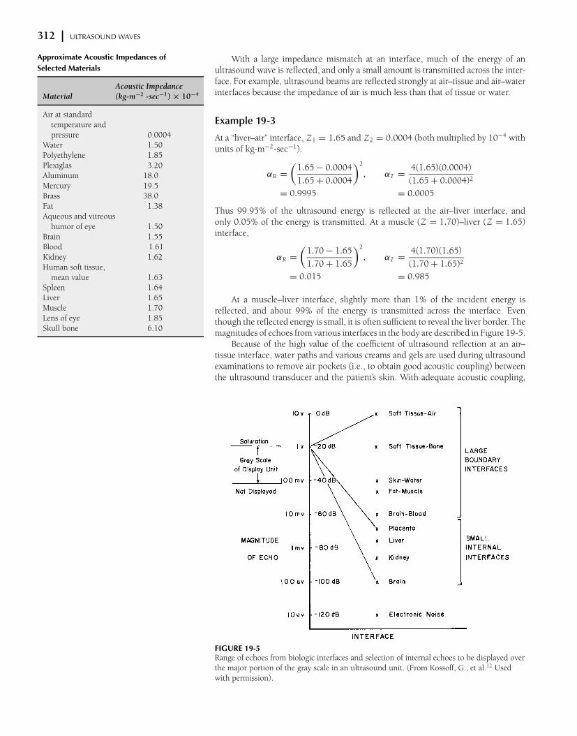
At a muscle–liver interface, slightly more than 1% of the incident energy isreflected, and about 99% of the energy is transmitted across the interface. Eventhough the reflected energy is small, it is often sufficient to reveal the liver border. Themagnitudes of echoes from various interfaces in the body are described in Figure 19-5.
Because of the high value of the coefficient of ultrasound reflection at an air–tissue interface, water paths and various creams and gels are used during ultrasoundexaminations to remove air pockets (i.e., to obtain good acoustic coupling) betweenthe ultrasound transducer and the patient’s skin. With adequate acoustic coupling,
FIGURE 19-5Range of echoes from biologic interfaces and selection of internal echoes to be displayed over
the major portion of the gray scale in an ultrasound unit. (From Kossoff, G., et al.12 Used
with permission).

REFRACTION x 313
MARGIN FIGURE 19-3Ultrasound reflection at an interface, where the
angle of incidence θi equals the angle of
reflection θr .
MARGIN FIGURE 19-4Refraction of ultrasound at an interface, where the
ratio of the velocities of ultrasound in the two
media is related to the sine of the angles of
incidence and refraction.
MARGIN FIGURE 19-5For an incidence angle θc equal to the critical
angle, refraction causes the sound to be
transmitted along the surface of the material. For
incidence angles greater than θc , sound
transmission across the interface is prevented
by refraction.
the ultrasound waves will enter the patient with little reflection at the skin surface.Similarly, strong reflections of ultrasound occur at the boundary between the chestwall and the lungs and at the millions of air–tissue interfaces within the lungs. Becauseof the large impedance mismatch at these interfaces, efforts to use ultrasound as adiagnostic tool for the lungs have been unrewarding. The impedance mismatch isalso high between soft tissues and bone, and the use of ultrasound to identify tissuecharacteristics in regions behind bone has had limited success.
The discussion of ultrasound reflection above assumes that the ultrasound beamstrikes the reflecting interface at a right angle. In the body, ultrasound impinges uponinterfaces at all angles. For any angle of incidence, the angle at which the reflectedultrasound energy leaves the interface equals the angle of incidence of the ultrasoundbeam; that is,
Angle of incidence = Angle of reflection
In a typical medical examination that uses reflected ultrasound and a transducerthat both transmits and detects ultrasound, very little reflected energy will be detectedif the ultrasound strikes the interface at an angle more than about 3 degrees fromperpendicular. A smooth reflecting interface must be essentially perpendicular to theultrasound beam to permit visualization of the interface.
¥ REFRACTION
As an ultrasound beam crosses an interface obliquely between two media, its directionis changed (i.e., the beam is bent). If the velocity of ultrasound is higher in the secondmedium, then the beam enters this medium at a more oblique (less steep) angle. Thisbehavior of ultrasound transmitted obliquely across an interface is termed refraction.The relationship between incident and refraction angles is described by Snell’s law:
Sine of incidence angle
Sine of refractive angle=
Velocity inincidence medium
Velocity inrefractive medium
sin θi
sin θr
=c i
cr
(19-4)
Two conditions are required for
refraction to occur: (1) The sound beam
must strike an interface at an angle
other than 90◦; (2) the speed of sound
must differ on opposite sides of the
interface.
For example, an ultrasound beam incident obliquely upon an interface between mus-cle (velocity 1580 m/sec) and fat (velocity 1475 m/sec) will enter the fat at a steeperangle.
If an ultrasound beam impinges very obliquely upon a medium in which theultrasound velocity is higher, the beam may be refracted so that no ultrasound energyenters the medium. The incidence angle at which refraction causes no ultrasoundto enter a medium is termed the critical angle θc . For the critical angle, the angle ofrefraction is 90 degrees, and the sine of 90 degrees is 1. From Eq. (19-4),
sin θc
sin 90◦=
c i
cr
but
sin 90◦= 1
therefore
θc = sin−1[c i /cr ]
where sin−1, or arcsin, refers to the angle whose sine is c i /cr . For any particularinterface, the critical angle depends only upon the velocity of ultrasound in the twomedia separated by the interface.

314 x ULTRASOUND WAVES
MARGIN FIGURE 19-6Lateral displacement of an ultrasound beam as it
traverses a slab interposed in an otherwise
homogeneous medium.
Refraction is a principal cause of artifacts in clinical ultrasound images. In MarginFigure 19-6, for example, the ultrasound beam is refracted at a steeper angle as itcrosses the interface between medium 1 and 2 (c1 > c2). As the beam emerges frommedium 2 and reenters medium 1, it resumes its original direction of motion. The pres-ence of medium 2 simply displaces the ultrasound beam laterally for a distance thatdepends upon the difference in ultrasound velocity and density in the two media andupon the thickness of medium 2. Suppose a small structure below medium 2 is visual-ized by reflected ultrasound. The position of the structure would appear to the vieweras an extension of the original direction of the ultrasound through medium 1. In thismanner, refraction adds spatial distortion and resolution loss to ultrasound images.
¥ ABSORPTION
American Institute of Ultrasound in
Medicine Safety Statement on
Diagnostic Ultrasound has been in use
since the early 1950s. Given its known
benefits and recognized efficacy for
medical diagnosis, including use during
human pregnancy, the American
Institute of Ultrasound in Medicine
hereby addresses the clinical safety of
such use as follows:
No confirmed biological effects on
patients or instrument operators
caused by exposure at intensities
typical of present diagnostic
ultrasound instruments have ever
been reported. Although the
possibility exists that such biological
effects may be identified in the
future, current data indicate that the
benefits to patients of the prudent
use of diagnostic ultrasound
outweigh the risks, if any, that may
be present.
Maximum ultrasound intensities
(mW/cm2) recommended by the U.S.
Food and Drug Administration for
various diagnostic applications. The
values are spatial-peak,
temporal-average (SPTA) values.5,13
Use (Intensity)max
Cardiac 430
Peripheral vessels 720
Ophthalmic 17
Abdominal 94
Fetal 94
Relaxation processes are the primary mechanisms of energy dissipation for anultrasound beam transversing tissue. These processes involve (a) removal of energyfrom the ultrasound beam and (b) eventual dissipation of this energy primarily asheat. As discussed earlier, ultrasound is propagated by displacement of molecules ofa medium into regions of compression and rarefaction. This displacement requiresenergy that is provided to the medium by the source of ultrasound. As the moleculesattain maximum displacement from an equilibrium position, their motion stops, andtheir energy is transformed from kinetic energy associated with motion to potentialenergy associated with position in the compression zone. From this position, themolecules begin to move in the opposite direction, and potential energy is gradu-ally transformed into kinetic energy. The maximum kinetic energy (i.e., the highestmolecular velocity) is achieved when the molecules pass through their original equi-librium position, where the displacement and potential energy are zero. If the kineticenergy of the molecule at this position equals the energy absorbed originally from theultrasound beam, then no dissipation of energy has occurred, and the medium is anideal transmitter of ultrasound. Actually, the conversion of kinetic to potential energy(and vice versa) is always accompanied by some dissipation of energy. Therefore, theenergy of the ultrasound beam is gradually reduced as it passes through the medium.This reduction is termed relaxation energy loss. The rate at which the beam energydecreases is a reflection of the attenuation properties of the medium.
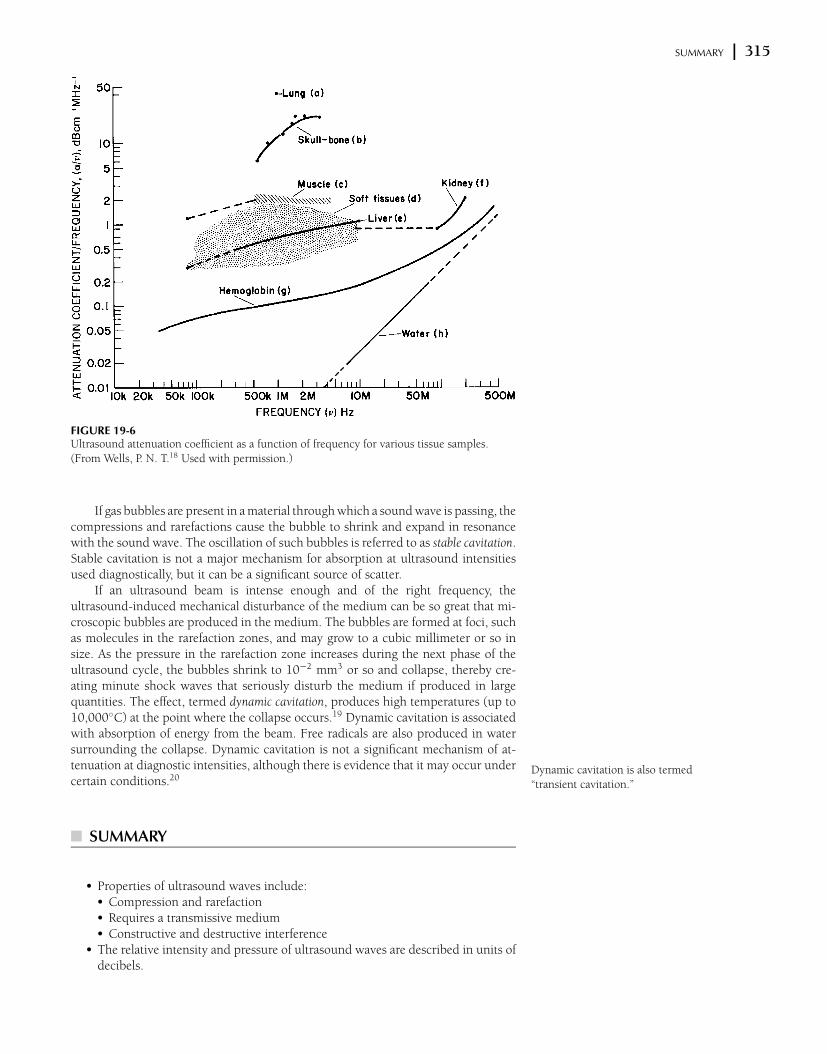
The effect of frequency on the attenuation of ultrasound in different media isdescribed in Table 19-5.14–18 Data in this table are reasonably good estimates of theinfluence of frequency on ultrasound absorption over the range of ultrasound fre-quencies used diagnostically. However, complicated structures such as tissue samplesoften exhibit a rather complex attenuation pattern for different frequencies, whichprobably reflects the existence of a variety of relaxation frequencies and other molecu-lar energy absorption processes that are poorly understood at present. These complexattenuation patterns are reflected in the data in Figure 19-6.
TABLE 19-5 Variation of Ultrasound Attenuation Coefficient α with Frequency in
Megahertz, Where α1 Is the Attenuation Coefficient at 1 MHz
Tissue Frequency Variation Material Frequency Variation
Blood α = α1 × v Lung α = α1 × v
Fat α = α1 × v Liver α = α1 × v
Muscle (across fibers) α = α1 × v Brain α = α1 × v
Muscle (along fibers) α = α1 × v Kidney α = α1 × v
Aqueous and vitreous Spinal cord α = α1× v
humor of eye α = α1 × v Water α = α1 × v2
Lens of eye α = α1 × v Caster oil α = α1 × v2
Skull bone α = α1 × v2 Lucite α = α1 × v
SUMMARY x 315
FIGURE 19-6Ultrasound attenuation coefficient as a function of frequency for various tissue samples.
(From Wells, P. N. T.18 Used with permission.)
If gas bubbles are present in a material through which a sound wave is passing, thecompressions and rarefactions cause the bubble to shrink and expand in resonancewith the sound wave. The oscillation of such bubbles is referred to as stable cavitation.Stable cavitation is not a major mechanism for absorption at ultrasound intensitiesused diagnostically, but it can be a significant source of scatter.
If an ultrasound beam is intense enough and of the right frequency, theultrasound-induced mechanical disturbance of the medium can be so great that mi-croscopic bubbles are produced in the medium. The bubbles are formed at foci, suchas molecules in the rarefaction zones, and may grow to a cubic millimeter or so insize. As the pressure in the rarefaction zone increases during the next phase of theultrasound cycle, the bubbles shrink to 10−2 mm3 or so and collapse, thereby cre-ating minute shock waves that seriously disturb the medium if produced in largequantities. The effect, termed dynamic cavitation, produces high temperatures (up to10,000◦C) at the point where the collapse occurs.19 Dynamic cavitation is associatedwith absorption of energy from the beam. Free radicals are also produced in watersurrounding the collapse. Dynamic cavitation is not a significant mechanism of at-tenuation at diagnostic intensities, although there is evidence that it may occur undercertain conditions.20
¥ SUMMARY
Dynamic cavitation is also termed
“transient cavitation.”
r Properties of ultrasound waves include:r Compression and rarefactionr Requires a transmissive mediumr Constructive and destructive interference
r The relative intensity and pressure of ultrasound waves are described in units ofdecibels.
316 x ULTRASOUND WAVES
r Ultrasound may be reflected or refracted at a boundary between two media.These properties are determined by the angle of incidence of the ultrasound andthe impedance mismatch at the boundary.
r Energy may be removed from an ultrasound beam by various processes, includ-ing relaxation energy loss.
r The presence of gas bubbles in a medium may give rise to stable and dynamiccavitation.
x PROBLEMS x19-1. Explain what is meant by a longitudinal wave, and describe how
an ultrasound wave is propagated through a medium.
*19-2. An ultrasound beam is attenuated by a factor of 20 in passing
through a medium. What is the attenuation of the medium in
decibels?
*19-3. Determine the fraction of ultrasound energy transmitted and re-
flected at interfaces between (a) fat and muscle and (b) lens and
aqueous and vitreous humor of the eye.
*19-4. What is the angle of refraction for an ultrasound beam incident
at an angle of 15 degrees from muscle into bone?
19-5. Explain why refraction contributes to resolution loss in ultra-
sound imaging.
*19-6. A region of tissue consists of 3 cm fat, 2 cm muscle (ultra-
sound propagated parallel to fibers), and 3 cm liver. What
is the approximate total energy loss of ultrasound in the
tissue?
∗For those problems marked with an asterisk, answers are provided on p. 493.
x REFERENCES x1. Zagzebski, J. Essentials of Ultrasound Physics. St. Louis, Mosby–Year Book,
1996.
2. Wells, P. N. T. Biomedical Ultrasonics. New York, Academic Press, 1977.
3. McDicken, W. Diagnostic Ultrasonics. New York, John Wiley & Sons, 1976.
4. Eisenberg, R. Radiology: An Illustrated History. St. Louis, Mosby–Year Book,
1992, pp. 452–466.
5. Bushong, S. Diagnostic Ultrasound. New York, McGraw-Hill, 1999.
6. Palmer, P. E. S. Manual of Diagnostic Ultrasound. Geneva, Switzerland, World
Health Organization, 1995.
7. Graff KF. Ultrasonics: Historical aspects. Presented at the IEEE Symposium on
Sonics and Ultrasonics, Phoenix, October 26–28, 1977.
8. Hendee, W. R., and Holmes, J. H. History of Ultrasound Imaging, in Fullerton,
G. D., and Zagzebski, J. A. (eds.), Medical Physics of CT and Ultrasound. New
York: American Institute of Physics, 1980.
9. Hendee, W. R. Cross sectional medical imaging: A history. Radiographics 1989;
9:1155–1180.
10. Kinsler, L. E., et al. Fundamentals of Acoustics, 3rd edition New York, John
Wiley & Sons, 1982, pp. 115–117.
11. ter Haar GR. In CR Hill (ed): Physical Principles of Medical Ultrasonics.
Chichester, England, Ellis Horwood/Wiley, 1986.
12. Kossoff, G., Garrett, W. J., Carpenter, D. A., Jellins, J., Dadd, M. J. Principles
and classification of soft tissues by grey scale echography. Ultrasound Med.
Biol. 1976; 2:89–111.
13. Thrush, A., and Hartshorne, T. Peripheral Vascular Ultrasound. London,
Churchill-Livingstone, 1999.
14. Chivers, R., and Hill, C. Ultrasonic attenuation in human tissues. Ultrasound
Med. Biol. 1975; 2:25.
15. Dunn, F., Edmonds, P., and Fry, W. Absorption and Dispersion of Ultrasound
in Biological Media, in H. Schwan (ed.), Biological Engineering. New York,
McGraw-Hill, 1969, p. 205
16. Powis, R. L., and Powis, W. J. A Thinker’s Guide to Ultrasonic Imaging. Baltimore,
Urban & Schwarzenberg, 1984.
17. Kertzfield, K., and Litovitz, T. Absorption and Dispersion of Ultrasonic Waves.
New York, Academic Press, 1959.
18. Wells, P. N. T. Review: Absorption and dispersion of ultrasound in biological
tissue. Ultrasound Med Biol 1975; 1:369–376.
19. Suslick, K. S. (ed.). Ultrasound, Its Chemical, Physical and Biological Effects.
New York, VCH Publishers, 1988.
20. Apfel, R. E. Possibility of microcavitation from diagnostic ultrasound. Trans.
IEEE 1986; 33:139–142.
C H A P T E R
20ULTRASOUND TRANSDUCERS
OBJECTIVES 318
INTRODUCTION 318
PIEZOELECTRIC EFFECT 318
TRANSDUCER DESIGN 319
FREQUENCY RESPONSE OF TRANSDUCERS 320
ULTRASOUND BEAMS 321
Wave Fronts 321
Beam Profiles 323
Focused Transducers 325
Doppler Probes 326
Multiple-Element Transducers 326
Transducer Damage 327
PROBLEMS 329
SUMMARY 329
REFERENCES 329
Medical Imaging Physics, Fourth Edition, by William R. Hendee and E. Russell RitenourISBN: 0-471-38226-4 Copyright C© 2002 Wiley-Liss, Inc. 317
318 x ULTRASOUND TRANSDUCERS
¥ OBJECTIVES
After studying this chapter, the reader should be able to:
r Explain the piezoelectric effect and its use in ultrasound transducers.r Characterize the properties of an ultrasound transducer, including those that
influence the resonance frequency.r Describe the properties of an ultrasound beam, including the Fresnel and Fraun-
hofer zones.r Delineate the characteristics of focused ultrasound beams and various ultrasound
probes.r Identify different approaches to multitransducer arrays and the advantages of
each.
¥ INTRODUCTION
A transducer is any device that converts one form of energy into another. An ultra-sound transducer converts electrical energy into ultrasound energy and vice versa.Transducers for ultrasound imaging consist of one or more piezoelectric crystalsor elements. The basic properties of ultrasound transducers (resonance, frequencyresponse, focusing, etc.) can be illustrated in terms of single-element transducers.However, imaging is often preformed with multiple-element “arrays” of piezoelectriccrystals.
¥ PIEZOELECTRIC EFFECT
The piezoelectric effect is exhibited by certain crystals that, in response to appliedpressure, develop a voltage across opposite surfaces.1–3 This effect is used to pro-duce an electrical signal in response to incident ultrasound waves. The magnitudeof the electrical signal varies directly with the wave pressure of the incident ultra-sound. Similarly, application of a voltage across the crystal causes deformation of thecrystal—either compression or extension depending upon the polarity of the voltage.This deforming effect, termed the converse piezoelectric effect, is used to produce anultrasound beam from a transducer.
The piezoelectric effect was first
described by Pierre and Jacques Curie
in 1880.
The movement of the surface of a
piezoelectric crystal used in diagnostic
imaging is on the order of a few
micrometers (10−3 mm) at a rate of
several million times per second. This
movement, although not discernible to
the naked eye, is sufficient to transmit
ultrasound energy into the patient.
An ultrasound transducer driven by a
continuous alternating voltage
produces a continuous ultrasound
wave. Continuous-wave (CW)
transducers are used in CW Doppler
ultrasound. A transducer driven by a
pulsed alternating voltage produces
ultrasound bursts that are referred to
collectively as pulse-wave ultrasound.
Pulsed ultrasound is used in most
applications of ultrasound imaging.
Pulsed Doppler uses ultrasound pulses
of longer duration than those employed
in pulse-wave imaging.
Many crystals exhibit the piezoelectric effect at low temperatures, but are unsuit-able as ultrasound transducers because their piezoelectric properties do not exist atroom temperature. The temperature above which a crystal’s piezoelectric propertiesdisappear is known as the Curie point of the crystal.
A common definition of the efficiency of a transducer is the fraction of appliedenergy that is converted to the desired energy mode. For an ultrasound transducer,this definition of efficiency is described as the electromechanical coupling coefficientkc . If mechanical energy (i.e., pressure) is applied, we obtain
k2c =
Mechanical energy converted to electrical energy
Applied mechanical energy
If electrical energy is applied, we obtain
k2c =
Electrical energy converted to mechanical energy
Applied electrical energy
Values of kc for selected piezoelectric crystals are listed in Table 20-1.Essentially all diagnostic ultrasound units use piezoelectric crystals for the genera-
tion and detection of ultrasound. A number of piezoelectric crystals occur in nature(e.g., quartz, Rochelle salts, lithium sulfate, tourmaline, and ammonium dihydrogenphosphate [ADP]). However, crystals used clinically are almost invariable man-made

TRANSDUCER DESIGN x 319
TABLE 20-1 Properties of Selected Piezoelectric Crystals
Electromechanical Curie Point
Materials Coupling Coefficient (Kc) (◦C)
Quartz 0.11 550
Rochelle salt 0.78 45
Barium titanate 0.30 120
Lead zirconate titanate (PZT-4) 0.70 328
Lead zirconate titanate (PZT-5) 0.70 365
ceramic ferroelectrics. The most common man-made crystals are barium titanate, leadmetaniobate, and lead zirconate titanate (PZT).
In some transducers of newer design,
the piezoelectric ceramic is mixed with
epoxy to form a composite ceramic.
Composite ceramics have several
performance advantages in comparison
with conventional ceramics.4
The components of an ultrasound
transducer include the
r Piezoelectric crystalr Damping materialr Electrodesr Housingr Matching layerr Insulating cover
¥ TRANSDUCER DESIGN
The piezoelectric crystal is the functional component of an ultrasound transducer.A crystal exhibits its greatest response at the resonance frequency. The resonance fre-quency is determined by the thickness of the crystal (the dimension of the crystalalong the axis of the ultrasound beam). As the crystal goes through a complete cy-cle from contraction to expansion to the next contraction, compression waves movetoward the center of the crystal from opposite crystal faces. If the crystal thicknessequals one wavelength of the sound waves, the compressions arrive at the oppositefaces just as the next crystal contraction begins. The compression waves oppose thecontraction and “dampen” the crystal’s response. Therefore it is difficult (i.e., energywould be wasted) to “drive” a crystal with a thickness of one wavelength. If the crys-tal thickness equals half of the wavelength, a compression wave reaches the oppositecrystal face just as expansion is beginning to occur. Each compression wave producedin the contraction phase aids in the expansion phase of the cycle. A similar result isobtained for any odd multiple of half wavelengths (e.g., 3λ/2, 5λ/2), with the crystalprogressing through more than one cycle before a given compression wave arrivesat the opposite face. Additional crystal thickness produces more attenuation, so themost efficient operation is achieved for a crystal with a thickness equal to half thewavelength of the desired ultrasound. A crystal of half-wavelength thickness resonatesat a frequency ν:
ν =c
λ
=c
2t
where λ = 2t
The transducer described here is a
“single-element” transducer. Such a
transducer is used in some
ophthalmological, m-mode, and pulsed
Doppler applications. Most other
applications of ultrasound employ one
of the multielement transducers
described later in this chapter.
High-frequency ultrasound transducers
employ thin (<1 mm) piezoelectric
crystals. A thicker crystal yields
ultrasound of lower frequency.
Example 20-1
For a 1.5-mm-thick quartz disk (velocity of ultrasound in quartz = 5740 m/sec),what is the resonance frequency?
ν =5740 m/sec
2(0.0015 m)
= 1.91 MHz
To establish electrical contract with a piezoelectric crystal, faces of the crystal arecoated with a thin conducting film, and electric contacts are applied. The crystal ismounted at one end of a hollow metal or metal-lined plastic cylinder, with the frontface of the crystal coated with a protective plastic that provides efficient transfer ofsound between the crystal and the body. The plastic coating at the face of the crystal has

320 x ULTRASOUND TRANSDUCERS
MARGIN FIGURE 20-1Typical ultrasound transducer.
MARGIN FIGURE 20-2Frequency–response curves for undamped (sharp
curve) and damped (broad curve) transducers.
a thickness of 1/4λ and is called a quarter-wavelength matching layer. A 1/4λ thicknessmaximizes energy transfer from the transducer to the patient. An odd multiple ofone-quarter wavelengths would perform the same function, but the greater thicknessof material would increase attenuation. Therefore, a single one-quarter wavelengththickness commonly is used for the matching layer. The front face of the crystal isconnected through the cylinder to ground potential. The remainder of the crystal iselectrically and acoustically insulated from the cylinder.
With only air behind the crystal, ultrasound transmitted into the cylinder fromthe crystal is reflected from the cylinder’s opposite end. The reflected ultrasound re-inforces the ultrasound propagated in the forward direction from the transducer. Thisreverberation of ultrasound in the transducer itself contributes energy to the ultra-sound beam. It also extends the pulse duration (the time over which the ultrasoundpulse is produced). Extension of the pulse duration (sometimes called temporal pulselength) is no problem in some clinical uses of ultrasound such as continuous-wave andpulsed-Doppler applications. For these purposes, ultrasound probes with air-backedcrystals may be used. However, most ultrasound imaging applications utilize shortpulses of ultrasound, and suppression of ultrasound reverberation in the transduceris desirable. Suppression or “damping” of reverberation is accomplished by filling thetransducer cylinder with a backing material such as tungsten powder embedded inepoxy resin. Sometimes, rubber is added to the backing to increase the absorptionof ultrasound. Often, the rear surface of the backing material is sloped to preventdirect reflection of ultrasound pulses back to the crystal. The construction of a typicalultrasound transducer is illustrated in the margin. The crystal may be flat, as shownin the drawing, or curved to focus the ultrasound beam.
Damping the reverberation of an
ultrasound transducer is similar to
packing foam rubber around a ringing
bell.
The few reverberation cycles after each
voltage pulse applied to a damped
ultrasound crystal is described as the
ringdown of the crystal.
As a substitute for physical damping with selected materials placed behind thecrystal, electronic damping may be used. In certain applications, including those thatuse a small receiving transducer, a resistor connecting the two faces of an air-backedcrystal may provide adequate damping. Another approach, termed dynamic damping,uses an initial electrical pulse to stimulate the transducer, followed immediately by avoltage pulse of opposite polarity to suppress continuation of transducer action.
Ultrasound frequencies from 2–10 MHz
are used for most diagnostic medical
applications.
¥ FREQUENCY RESPONSE OF TRANSDUCERS
An ultrasound transducer is designed to be maximally sensitive to ultrasound of aparticular frequency, termed the resonance frequency of the transducer. The resonancefrequency is determined principally by the thickness of the piezoelectric crystal. Thincrystals yield high resonance frequencies, and vice versa. The resonance frequencyis revealed by a curve of transducer response plotted as a function of ultrasoundfrequency. In the illustration in the margin, the frequency response characteristics oftwo transducers are illustrated. The curve for the undamped transducer displays asharp frequency response over a limited frequency range. Because of greater energyabsorption in the damped transducer, the frequency response is much broader andnot so sharply peaked at the transducer resonance frequency. On the curve for theundamped transducer, points ν1 and ν3 represent frequencies on either side of theresonance frequency where the response has diminished to half. These points arecalled the half-power points, and they encompass a range of frequencies termedthe bandwidth of the transducer. The ratio of the “center,” or resonance frequencyν2, to the bandwidth (ν3 − νt ) is termed the Q value of the transducer. The Qvalue describes the sharpness of the frequency response curve, with a high Q valueindicating a sharply-peaked frequency response.
Q value =ν2
ν3 − ν1
Transducers used in ultrasound imaging must furnish short ultrasound pulsesand respond to returning echoes over a wide range of frequencies. For these reasons,heavily damped transducers with low Q values (e.g., 2 to 3) are usually desired.
ULTRASOUND BEAMS x 321
(a)
(b)
MARGIN FIGURE 20-3Typical long (A) and short (B) ultrasound pulses.
Because part of the damping is provided by the crystal itself, crystals such as PZT(lead zirconate titanate) or lead metaniobate with high internal damping and low Qvalues are generally preferred for imaging.
The resonance frequency ν2 is near the
value posted on the imaging system for
the transducer. For example, an
individual “3.5”-MHz transducer may
have an actual resonance frequency of
3.489 MHz.
The efficiency with which an ultrasound beam is transmitted from a transducerinto a medium (and vice versa) depends on how well the transducer is coupled tothe medium. If the acoustic impedance of the coupling medium is not too differentfrom that of either the transducer or the medium and if the thickness of the couplingmedium is much less than the ultrasound wavelength, then the ultrasound is trans-mitted into the medium with little energy loss. Transmission with almost no energyloss is accomplished, for example, with a thin layer of oil placed between transducerand skin during a diagnostic ultrasound examination. Transmission with minimumenergy loss occurs when the impedance of the coupling medium is intermediate be-tween the impedances of the crystal and the medium. The ideal impedance of thecoupling medium is
Zcoupling medium =
√
Z transducer × Zmedium
Coupling of the transducer to the
transmitting medium affects the size of
the electrical signals generated by
returning ultrasound pulses.
Two methods are commonly used to generate ultrasound beams. For continuous-wave beams, an oscillating voltage is applied with a frequency equal to that desiredfor the ultrasound beam. A similar voltage of prescribed duration is used to generatelong pulses of ultrasound energy, as shown in the margin (A). For clinical ultrasoundimaging, short pulses usually are preferred. These pulses are produced by shockingthe crystal into mechanical oscillation by a momentary change in the voltage acrossthe crystal. The oscillation is damped quickly by the methods described earlier tofurnish ultrasound pulses as short as half a cycle. The duration of a pulse usuallyis defined as the number of half cycles in the pulse with an amplitude greater thanone fourth of peak amplitude. The effectiveness of damping is described by the pulsedynamic range, defined as the ratio of the peak amplitude of the pulse divided by theamplitude of ripples following the pulse. A typical ultrasound pulse of short durationis illustrated in the margin (B).
Ultrasound from a point source creates
spherical wave fronts. Ultrasound from
a two-dimensional extended source
creates planar wavefronts.
¥ ULTRASOUND BEAMS
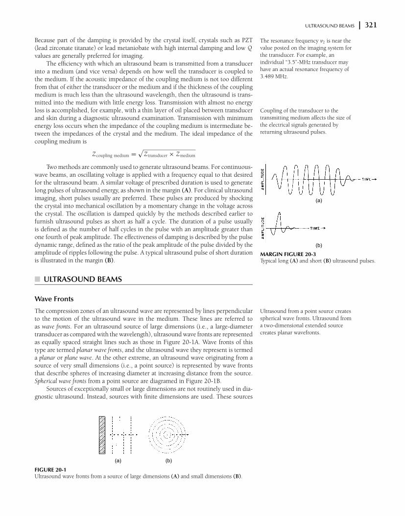
Wave Fronts
The compression zones of an ultrasound wave are represented by lines perpendicularto the motion of the ultrasound wave in the medium. These lines are referred toas wave fronts. For an ultrasound source of large dimensions (i.e., a large-diametertransducer as compared with the wavelength), ultrasound wave fronts are representedas equally spaced straight lines such as those in Figure 20-1A. Wave fronts of thistype are termed planar wave fronts, and the ultrasound wave they represent is termeda planar or plane wave. At the other extreme, an ultrasound wave originating from asource of very small dimensions (i.e., a point source) is represented by wave frontsthat describe spheres of increasing diameter at increasing distance from the source.Spherical wave fronts from a point source are diagramed in Figure 20-1B.
Sources of exceptionally small or large dimensions are not routinely used in dia-gnostic ultrasound. Instead, sources with finite dimensions are used. These sources
(a) (b)
FIGURE 20-1Ultrasound wave fronts from a source of large dimensions (A) and small dimensions (B).
322 x ULTRASOUND TRANSDUCERS
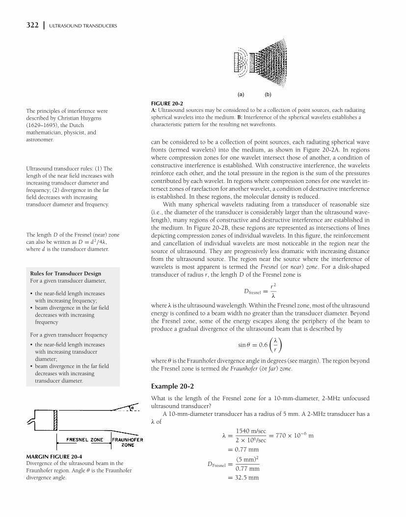
(a) (b)
FIGURE 20-2A: Ultrasound sources may be considered to be a collection of point sources, each radiating
spherical wavelets into the medium. B: Interference of the spherical wavelets establishes a
characteristic pattern for the resulting net wavefronts.
MARGIN FIGURE 20-4Divergence of the ultrasound beam in the
Fraunhofer region. Angle θ is the Fraunhofer
divergence angle.
can be considered to be a collection of point sources, each radiating spherical wavefronts (termed wavelets) into the medium, as shown in Figure 20-2A. In regionswhere compression zones for one wavelet intersect those of another, a condition ofconstructive interference is established. With constructive interference, the waveletsreinforce each other, and the total pressure in the region is the sum of the pressurescontributed by each wavelet. In regions where compression zones for one wavelet in-tersect zones of rarefaction for another wavelet, a condition of destructive interferenceis established. In these regions, the molecular density is reduced.
The principles of interference were
described by Christian Huygens
(1629–1695), the Dutch
mathematician, physicist, and
astronomer.
With many spherical wavelets radiating from a transducer of reasonable size(i.e., the diameter of the transducer is considerably larger than the ultrasound wave-length), many regions of constructive and destructive interference are established inthe medium. In Figure 20-2B, these regions are represented as intersections of linesdepicting compression zones of individual wavelets. In this figure, the reinforcementand cancellation of individual wavelets are most noticeable in the region near thesource of ultrasound. They are progressively less dramatic with increasing distancefrom the ultrasound source. The region near the source where the interference ofwavelets is most apparent is termed the Fresnel (or near) zone. For a disk-shapedtransducer of radius r, the length D of the Fresnel zone is
Dfresnel =r 2
λ
where λ is the ultrasound wavelength. Within the Fresnel zone, most of the ultrasoundenergy is confined to a beam width no greater than the transducer diameter. Beyondthe Fresnel zone, some of the energy escapes along the periphery of the beam toproduce a gradual divergence of the ultrasound beam that is described by
sin θ = 0.6
(
λ
r
)
where θ is the Fraunhofer divergence angle in degrees (see margin). The region beyondthe Fresnel zone is termed the Fraunhofer (or far) zone.
Ultrasound transducer rules: (1) The
length of the near field increases with
increasing transducer diameter and
frequency; (2) divergence in the far
field decreases with increasing
transducer diameter and frequency.
The length D of the Fresnel (near) zone
can also be written as D = d 2/4λ,
where d is the transducer diameter.
Rules for Transducer Design
For a given transducer diameter,
r the near-field length increases
with increasing frequency;r beam divergence in the far field
decreases with increasing
frequency
For a given transducer frequency
r the near-field length increases
with increasing transducer
diameter;r beam divergence in the far field
decreases with increasing
transducer diameter.Example 20-2
What is the length of the Fresnel zone for a 10-mm-diameter, 2-MHz unfocusedultrasound transducer?
A 10-mm-diameter transducer has a radius of 5 mm. A 2-MHz transducer has aλ of
λ =1540 m/sec
2 × 10⁶/sec= 770 × 10−6 m
= 0.77 mm
DFresnel =(5 mm)2
0.77 mm
= 32.5 mm
ULTRASOUND BEAMS x 323
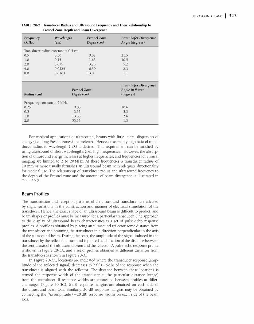
TABLE 20-2 Transducer Radius and Ultrasound Frequency and Their Relationship to
Fresnel Zone Depth and Beam Divergence
Frequency Wavelength Fresnel Zone Fraunhofer Divergence
(MHz) (cm) Depth (cm) Angle (degrees)
Transducer radius constant at 0.5 cm
0.5 0.30 0.82 21.5
1.0 0.15 1.63 10.5
2.0 0.075 3.25 5.2
4.0 0.0325 6.50 2.3
8.0 0.0163 13.0 1.1
Fraunhofer Divergence
Fresnel Zone Angle in Water
Radius (cm) Depth (cm) (degrees)
Frequency constant at 2 MHz
0.25 0.83 10.6
0.5 3.33 5.3
1.0 13.33 2.6
2.0 53.33 1.3
For medical applications of ultrasound, beams with little lateral dispersion ofenergy (i.e., long Fresnel zones) are preferred. Hence a reasonably high ratio of trans-ducer radius to wavelength (r /λ) is desired. This requirement can be satisfied byusing ultrasound of short wavelengths (i.e., high frequencies). However, the absorp-tion of ultrasound energy increases at higher frequencies, and frequencies for clinicalimaging are limited to 2 to 20 MHz. At these frequencies a transducer radius of10 mm or more usually furnishes an ultrasound beam with adequate directionalityfor medical use. The relationship of transducer radius and ultrasound frequency tothe depth of the Fresnel zone and the amount of beam divergence is illustrated inTable 20-2.
Beam Profiles
The transmission and reception patterns of an ultrasound transducer are affectedby slight variations in the construction and manner of electrical stimulation of thetransducer. Hence, the exact shape of an ultrasound beam is difficult to predict, andbeam shapes or profiles must be measured for a particular transducer. One approachto the display of ultrasound beam characteristics is a set of pulse-echo responseprofiles. A profile is obtained by placing an ultrasound reflector some distance fromthe transducer and scanning the transducer in a direction perpendicular to the axisof the ultrasound beam. During the scan, the amplitude of the signal induced in thetransducer by the reflected ultrasound is plotted as a function of the distance betweenthe central axis of the ultrasound beam and the reflector. A pulse-echo response profileis shown in Figure 20-3A, and a set of profiles obtained at different distances fromthe transducer is shown in Figure 20-3B.
In Figure 20-3A, locations are indicated where the transducer response (amp-litude of the reflected signal) decreases to half (−6 dB) of the response when thetransducer is aligned with the reflector. The distance between these locations istermed the response width of the transducer at the particular distance (range)from the transducer. If response widths are connected between profiles at differ-ent ranges (Figure 20-3C), 6-dB response margins are obtained on each side ofthe ultrasound beam axis. Similarly, 20-dB response margins may be obtained byconnecting the 1/10 amplitude (−20 dB) response widths on each side of the beamaxis.
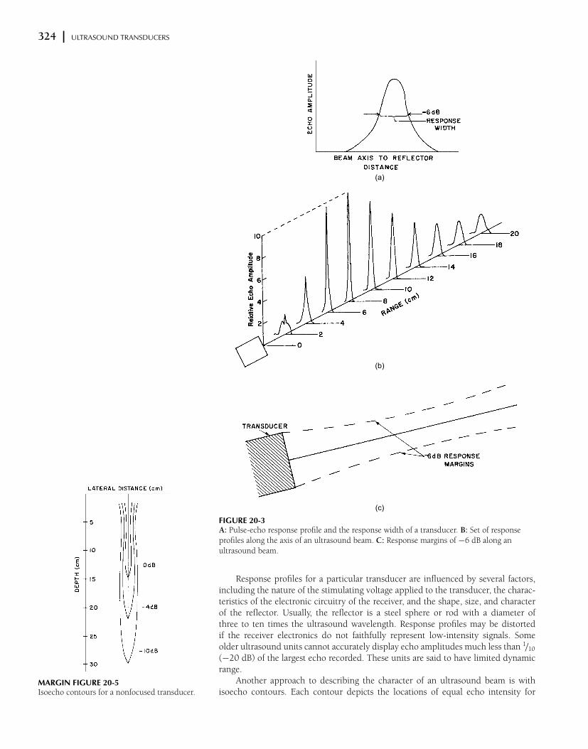
324 x ULTRASOUND TRANSDUCERS
(a)
(b)
(c)
FIGURE 20-3A: Pulse-echo response profile and the response width of a transducer. B: Set of response
profiles along the axis of an ultrasound beam. C: Response margins of −6 dB along an
ultrasound beam.
MARGIN FIGURE 20-5Isoecho contours for a nonfocused transducer.
Response profiles for a particular transducer are influenced by several factors,including the nature of the stimulating voltage applied to the transducer, the charac-teristics of the electronic circuitry of the receiver, and the shape, size, and characterof the reflector. Usually, the reflector is a steel sphere or rod with a diameter ofthree to ten times the ultrasound wavelength. Response profiles may be distortedif the receiver electronics do not faithfully represent low-intensity signals. Someolder ultrasound units cannot accurately display echo amplitudes much less than 1/10
(−20 dB) of the largest echo recorded. These units are said to have limited dynamicrange.
Another approach to describing the character of an ultrasound beam is withisoecho contours. Each contour depicts the locations of equal echo intensity for

ULTRASOUND BEAMS x 325
MARGIN FIGURE 20-6Side lobes of an ultrasound beam.
MARGIN FIGURE 20-7Focused transducer.
MARGIN FIGURE 20-8Focusing and defocusing mirrors.
MARGIN FIGURE 20-9Focusing and defocusing lenses.
the ultrasound beam. At each of these locations, a reflecting object will be detectedwith equal sensitivity. The approach usually used to measure isoecho contours isto place a small steel ball at a variety of positions in the ultrasound beam and toidentify locations where the reflected echoes are equal. Connecting these locationswith lines yields isoecho contours such as those in the margin, where the region ofmaximum sensitivity at a particular depth is labeled 0 dB, and isoecho contours oflesser intensity are labeled −4 dB, −10 dB, and so on. Isoecho contours help depict thelateral resolution of a transducer, as well as variations in lateral resolution with depthand with changes in instrument settings such as beam intensity, detector amplifiergain, and echo threshold.
Accompanying a primary ultrasound beam are small beams of greatly reducedintensity that are emitted at angles to the primary beam. These small beams, termedside lobes (see margin), are caused by vibratory modes of the transducer in thetransverse plane. Side lobes can produce image artifacts in regions near the transducer,if a particularly echogenic material, such as a biopsy needle, is present.
Side lobes can be reduced further by
the process of apodization, in which the
voltage applied to the transducer is
diminished from the center to the
periphery.
The preceding discussion covers general-purpose, flat-surfaced transducers. Formost ultrasound applications, transducers with special shapes are preferred. Amongthese special-purpose transducers are focused transducers, double-crystal transdu-cers, ophthalmic probes, intravascular probes, esophageal probes, composite probes,variable-angle probes, and transducer arrays.
Focused Transducers
A focused ultrasound transducer produces a beam that is narrower at some dis-tance from the transducer face than its dimension at the face of the transducer.5,6 Inthe region where the beam narrows (termed the focal zone of the transducer), theultrasound intensity may be heightened by 100 times or more compared with theintensity outside of the focal zone. Because of this increased intensity, a much largersignal will be induced in a transducer from a reflector positioned in the focal zone.The distance between the location for maximum echo in the focal zone and the ele-ment responsible for focusing the ultrasound beam is termed the focal length of thetransducer.
Often, the focusing element is the piezoelectric crystal itself, which is shaped likea concave disk (see figure in margin). An ultrasound beam also may be focused withmirrors and refracting lenses. Focusing lenses and mirrors are capable of increasingthe intensity of an ultrasound beam by factors greater than 100. Focusing mirrors,usually constructed of tungsten-impregnated epoxy resin, are illustrated in the margin.Because the velocity of ultrasound generally is greater in a lens than in the surroundingmedium, concave ultrasound lenses are focusing, and convex ultrasound lenses aredefocusing (see margin). These effects are the opposite of those for the action of opticallenses on visible light. Ultrasound lenses usually are constructed of epoxy resins andplastics such as polystyrene.
For an ultrasound beam with a circular cross section, focusing characteristicssuch as pulse-echo response width and relative sensitivity along the beam axis dependon the wavelength of the ultrasound and on the focal length f and radius r of thetransducer or other focusing element. These variables may be used to distinguish thedegree of focusing of transducers by dividing the near field length r 2/λ by the focallength f . For cupped transducer faces on all but weakly focused transducers, the focallength of the transducer is equal to or slightly shorter than the radius of curvature ofthe transducer face. If a planoconcave lens with a radius of curvature r is attached tothe transducer face, then the focal length f is
f =r
1 − c M /c L
where c M and c L are the velocities of ultrasound in the medium and lens, respecti-vely.

326 x ULTRASOUND TRANSDUCERS
Degree of Focus of Transducers Expressed as a
Ratio of the Near-field Length r2/λ to the Focal
Length f
Near–Field Length
Degree of Focus Focal Length
Weak (r 2/λ)/ f ≤ 1.4
Medium weak 1.4 < (r 2/λ)/ f ≤ 6
Medium 6 < (r 2/λ)/ f ≤ 20
Strong 20 < (r 2/λ)/ f
The ratio f/d, where d = 2r = the
diameter of the transducer, is often
described as the f-number of the
transducer or other focusing element.
The length of the focal zone of a particular ultrasound beam is the distance overwhich a reasonable focus and pulse-echo response are obtained. One estimate of focalzone length is
Focal zone length = 10λ
(
f
d
)2
where d = 2r is the diameter of the transducer. These strongly focused transducersare also used for surgical applications of ultrasound where high ultrasound intensitiesin localized regions are needed for tissue destruction.
Doppler Probes
Transducers for continuous-wave Doppler ultrasound consist of separate transmittingand receiving crystals, usually oriented at slight angles to each other so that thetransmitting and receiving areas intersect at some distance in front of the transducer(see margin). Because a sharp frequency response is desired for a Doppler transducer,only a small amount of damping material is used.
Multiple-Element Transducers
Scanning of the patient may be accomplished by physical motion of a single-elementultrasound transducer. The motion of the transducer may be executed manually bythe sonographer or automatically with a mechanical system. Several methods formechanical scanning are shown in Figure 20-4. The scanning technique that uses anautomatic scanning mechanism for the transducer is referred to as mechanical sectorscanning.
(a) (b)
(c)
FIGURE 20-4Three methods of mechanical scanning of the ultrasound beam. A: Multiple piezoelectric
elements (P ) mounted on a rotating head. One element is energized at a time as it rotates
through the sector angle. B: Single piezoelectric element oscillating at high frequency.
C: Single piezoelectric element reflected from an oscillating acoustic mirror (M ).
MARGIN FIGURE 20-10Front (left) and side (right) views of a typical
Doppler transducer.
MARGIN FIGURE 20-11Linear array. (From Zagzebski, J. A.4 Used with
permission.)
Publisher's Note:Permission to reproduce this imageonline was not granted by thecopyright holder. Readers are kindlyasked to refer to the printed versionof this chapter.
ULTRASOUND BEAMS x 327
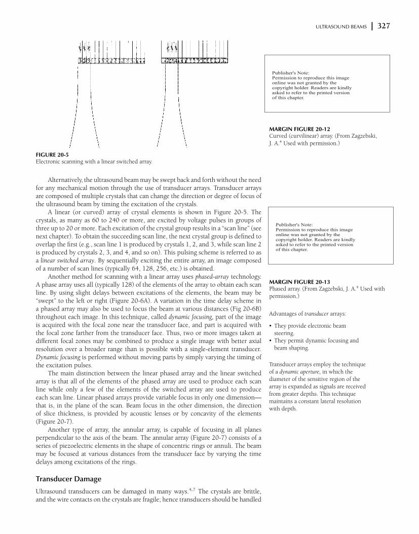
FIGURE 20-5Electronic scanning with a linear switched array.
MARGIN FIGURE 20-12Curved (curvilinear) array. (From Zagzebski,
J. A.4 Used with permission.)
MARGIN FIGURE 20-13Phased array. (From Zagzebski, J. A.4 Used with
permission.)
Alternatively, the ultrasound beam may be swept back and forth without the needfor any mechanical motion through the use of transducer arrays. Transducer arraysare composed of multiple crystals that can change the direction or degree of focus ofthe ultrasound beam by timing the excitation of the crystals.
A linear (or curved) array of crystal elements is shown in Figure 20-5. Thecrystals, as many as 60 to 240 or more, are excited by voltage pulses in groups ofthree up to 20 or more. Each excitation of the crystal group results in a “scan line” (seenext chapter). To obtain the succeeding scan line, the next crystal group is defined tooverlap the first (e.g., scan line 1 is produced by crystals 1, 2, and 3, while scan line 2is produced by crystals 2, 3, and 4, and so on). This pulsing scheme is referred to asa linear switched array. By sequentially exciting the entire array, an image composedof a number of scan lines (typically 64, 128, 256, etc.) is obtained.
Another method for scanning with a linear array uses phased-array technology.A phase array uses all (typically 128) of the elements of the array to obtain each scanline. By using slight delays between excitations of the elements, the beam may be“swept” to the left or right (Figure 20-6A). A variation in the time delay scheme ina phased array may also be used to focus the beam at various distances (Fig 20-6B)throughout each image. In this technique, called dynamic focusing, part of the imageis acquired with the focal zone near the transducer face, and part is acquired withthe focal zone farther from the transducer face. Thus, two or more images taken atdifferent focal zones may be combined to produce a single image with better axialresolution over a broader range than is possible with a single-element transducer.Dynamic focusing is performed without moving parts by simply varying the timing ofthe excitation pulses.
Advantages of transducer arrays:
r They provide electronic beam
steering.r They permit dynamic focusing and
beam shaping.
Transducer arrays employ the technique
of a dynamic aperture, in which the
diameter of the sensitive region of the
array is expanded as signals are received
from greater depths. This technique
maintains a constant lateral resolution
with depth.
The main distinction between the linear phased array and the linear switchedarray is that all of the elements of the phased array are used to produce each scanline while only a few of the elements of the switched array are used to produceeach scan line. Linear phased arrays provide variable focus in only one dimension—
that is, in the plane of the scan. Beam focus in the other dimension, the directionof slice thickness, is provided by acoustic lenses or by concavity of the elements(Figure 20-7).
Another type of array, the annular array, is capable of focusing in all planesperpendicular to the axis of the beam. The annular array (Figure 20-7) consists of aseries of piezoelectric elements in the shape of concentric rings or annuli. The beammay be focused at various distances from the transducer face by varying the timedelays among excitations of the rings.
Transducer Damage
Ultrasound transducers can be damaged in many ways.4,7 The crystals are brittle,and the wire contacts on the crystals are fragile; hence transducers should be handled
Publisher's Note:Permission to reproduce this imageonline was not granted by thecopyright holder. Readers are kindlyasked to refer to the printed versionof this chapter.
Publisher's Note:Permission to reproduce this imageonline was not granted by thecopyright holder. Readers are kindlyasked to refer to the printed versionof this chapter.
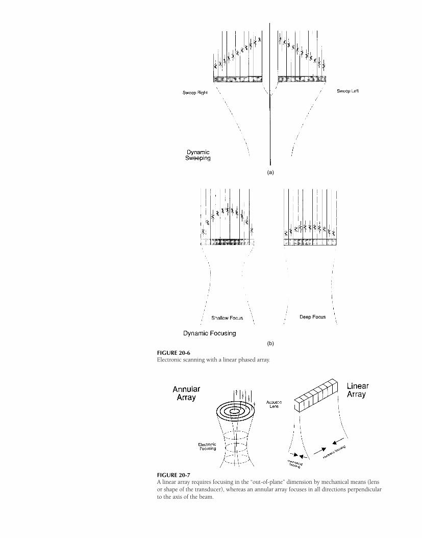
(a)
(b)
FIGURE 20-6Electronic scanning with a linear phased array.
FIGURE 20-7A linear array requires focusing in the “out-of-plane” dimension by mechanical means (lens
or shape of the transducer), whereas an annular array focuses in all directions perpendicular
to the axis of the beam.

REFERENCES x 329
carefully. Excessive voltages to the crystal should be avoided, and only watertightprobes should be immersed in water. A transducer should never be heated to a tem-perature near the Curie point of the piezoelectric crystal. Dropping a transducer,twisting, bending, and crushing the transducer cables, and other examples of mis-handling ultrasound transducers are frequent causes of dysfunction.
x PROBLEMS x20-1. Explain what is meant by the piezoelectric effect and the converse
piezoelectric effect.
*20-2. For a piezoelectric material with an ultrasound velocity of
6000 m/sec, what thickness should a disk-shaped crystal have
to provide an ultrasound beam with a frequency of 2.5 MHz?
20-3. What is meant by damping an ultrasound transducer, and why
is this necessary? What influence does damping have on the
frequency response of the transducer?
*20-4. What is the estimated focal zone length for a 2-MHz (λ =
0.075 cm) focused ultrasound transducer with an f-number
of 8?
20-5. A linear array can be electronically steering and focused. An an-
nular array can be electronically focused. Can an annular array
be electronically steered?
*For those problems marked with an asterisk, answers are provided on p. 493.
¥ SUMMARY
r The active element of an ultrasound transducer is a crystal that exhibits thepiezoelectric (receiver) and converse piezoelectric (transmitter) effect.
r The resonance frequency of a transducer is determined by the type of piezoelec-tric crystal and its thickness.
r The bandwidth of a transducer is expressed by its Q value.r The Fresnel zone, the area of minimum beam divergence in front of the trans-
ducer, has an axial dimension determined by r 2/λ.r The angle θ of divergence of the ultrasound beam in the Fraunhofer zone is
determined by sin θ = 0.6 (λ/r ).r The shape of an ultrasound beam may be described by response profiles or
isoecho contours.r Real-time ultrasound scans may be obtained with mechanical sector scanners or
multitransducer arrays.r Multitransducer arrays include linear switched arrays, linear phased arrays, and
annular arrays.
x REFERENCES x1. McDicken, W. Diagnostic Ultrasonics. New York, John Wiley & Sons, 1976,
p. 248.
2. Wells, P. Biomedical Ultrasonics. New York, Academic Press, 1977, p. 45.
3. Bumber, J. C., and Tristam, M. Diagnostic ultrasound, in Webb, S. (ed.), Physics
of Medical Imaging. Philadelphia, Adam Hilger, 1988, pp. 319–388.
4. Zagzebski, J. A. Essentials of Ultrasound Physics. St Louis, Mosby–Year Book,
1996.
5. Kossoff, G. Improved techniques in ultrasonic echography. Ultrasonics 1972,
10:221.
6. McElroy, J. Focused ultrasonic beams. Int J. Nondestruc Testing 1971;
3:27.
7. Hendee, W. R., et al. Design of a quality control program, in Hendee, W. (ed.),
The Selection and Performance of Radiologic Equipment. Baltimore, Williams &
Wilkins, 1985, pp 163–208.
C H A P T E R
21ULTRASOUND INSTRUMENTATION
OBJECTIVES 332
PRESENTATION MODES 332
A-Mode 332
B-Mode 332
M-Mode 333
TIME REQUIRED TO OBTAIN IMAGES 333
SYSTEM COMPONENTS 335
SIGNAL PROCESSING 335
Preprocessing 335
Postprocessing 336
DYNAMIC RANGE 337
ULTRASOUND IMAGE ARTIFACTS 338
Speckle 338
Shadowing and Enhancement 338
Multiple Pathway 338
Refraction 338
QUALITY CONTROL 338
Quality Control Tests 339
PROBLEMS 340
SUMMARY 341
REFERENCES 341
Medical Imaging Physics, Fourth Edition, by William R. Hendee and E. Russell RitenourISBN: 0-471-38226-4 Copyright C© 2002 Wiley-Liss, Inc. 331

332 x ULTRASOUND INSTRUMENTATION
A
B
C
Transducer
MARGIN FIGURE 21-1A-mode (amplitude mode) of ultrasound display.
An oscilloscope display records the amplitude of
echoes as a function of time or depth. Points A, B,
and C in the patient appear as peaks-A, B, and C
in the A-mode display.
¥ OBJECTIVES
After completing this chapter, the reader should be able to:
r Name three modes of ultrasound imaging.r Determine the time required to obtain an ultrasound image.r Define pulse repetition frequency and state the role it plays in frame rate.r Name the main components of an ultrasound imaging system.r Explain the preprocessing required to obtain digital data from ultrasound signals.r Define the term time gain compensation.r Explain how postprocessing is used to change the appearance of an ultrasound
image.r Describe several common artifacts in ultrasound images.r List several common ultrasound quality control tests.
All approaches to obtaining pictorial information with ultrasound depend on echo-ranging, the principle that the time required for return of a reflected signal indi-cates distance. Strategies for displaying echo-range information—amplitude A, bright-ness B, and motion M—are discussed in this chapter.
¥ PRESENTATION MODES
A-Mode
In the A-mode presentation of ultrasound images, echoes returning from the body aredisplayed as signals on an oscilloscope. The oscilloscope presents a graph of voltagerepresenting echo amplitude (hence the term “A-mode”) on the ordinate, or y-axis,as a function of time on the abscissa, or x-axis. With the assumption of a constantspeed of sound, time on the x-axis can be presented as distance from the ultrasoundtransducers (Margin Figure 21-1).
For each centimeter of depth,
ultrasound travels 2 cm, 1 cm “out” for
the transmitted pulse and 1 cm “back”
for the reflected pulse. With the
assumption of a speed of sound of
1540 m/sec for ultrasound in soft
tissue, the time that corresponds to
each centimeter of “depth” is
0.02 m
1540 m/sec= 0.000013 sec = 13 µsec
The result is a conversion factor of
13 µsec/cm for diagnostic ultrasound
that is used to convert time to distance
and vice versa.
This conversion factor is appropriate
for reflection imaging in soft tissue
where a speed of sound of 1540 m/sec
is assumed to be reasonably accurate.
A-mode reveals the location of echo-producing structures only in the direction ofthe ultrasound beam. It has been used in the past to localize echo-producing interfacessuch as midline structures in the brain (echoencephalography) and structures to beimaged in B-mode. A-mode displays are not found on most imaging systems usedtoday. The concept of A-mode is however, useful in explaining how pixels are obtainedfrom scan lines in B-mode imaging.
B-Mode
In B-mode presentation of pulse echo images (Margin Figure 21-2) the location ofecho-producing interfaces is displayed in two dimensions (x and y) on a video screen.The amplitude of each echo is represented by the brightness value at the xy location.High-amplitude echoes can be presented as either high brightness or low brightness
A-mode displays of a transcranial scan
(echoencephalography) were used until
the late 1970s to detect shifts of the
midline in the brain of newborns with
suspected hydrocephaly. This technique
has been replaced by B-mode real-time
scanning, computed tomography and
magnetic resonance imaging.
to provide either “white-on-black” or “black-on-white” presentations. Most images areviewed as white on black, so regions in the patient that are more echogenic correspondto regions in the image that are brighter (hence B for “brightness” mode).
B-mode images may be displayed as either “static” or “real-time” images. In staticimaging the image is compiled as the sound beam is scanned across the patient, andthe image presents a “snapshot” averaged over the time required to sweep the soundbeam. In real-time imaging, the image is also built up as the sound beam scans acrossthe patient, but the scanning is performed automatically and quickly, and one imagefollows another in quick succession. At image frequencies greater than approximately24 per second, the motion of moving structures seems continuous, even though itmay appear that the images are flickering (i.e., being flashed on and off). Imagesthat are refreshed at frequencies greater than approximately 48 per second are free offlicker.
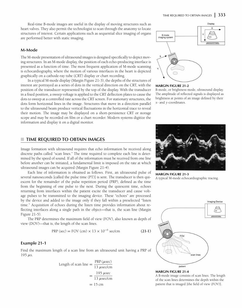
TIME REQUIRED TO OBTAIN IMAGES x 333
Transducer
MARGIN FIGURE 21-2B-mode, or brightness mode, ultrasound display.
The amplitude of reflected signals is displayed as
brightness at points of an image defined by their
x- and y-coordinates.
Real-time B-mode images are useful in the display of moving structures such asheart valves. They also permit the technologist to scan through the anatomy to locatestructures of interest. Certain applications such as sequential slice imaging of organsare performed better with static imaging.
M-Mode
The M-mode presentation of ultrasound images is designed specifically to depict mov-ing structures. In an M-mode display, the position of each echo-producing interface ispresented as a function of time. The most frequent application of M-mode scanningis echocardiography, where the motion of various interfaces in the heart is depictedgraphically on a cathode-ray tube (CRT) display or chart recording.
In a typical M-mode display (Margin Figure 21-3), the depths of the structures ofinterest are portrayed as a series of dots in the vertical direction on the CRT, with theposition of the transducer represented by the top of the display. With the transducerin a fixed position, a sweep voltage is applied to the CRT deflection plates to cause thedots to sweep at a controlled rate across the CRT screen. For stationary structures, thedots form horizontal lines in the image. Structures that move in a direction parallelto the ultrasound beam produce vertical fluctuations in the horizontal trace to revealtheir motion. The image may be displayed on a short-persistence CRT or storagescope and may be recorded on film or a chart recorder. Modern systems digitize theinformation and display it on a digital monitor.
MARGIN FIGURE 21-3A typical M-mode echocardiographic tracing.
¥ TIME REQUIRED TO OBTAIN IMAGES
Image formation with ultrasound requires that echo information be received alongdiscrete paths called “scan lines.” The time required to complete each line is deter-mined by the speed of sound. If all of the information must be received from one linebefore another can be initiated, a fundamental limit is imposed on the rate at whichultrasound images can be acquired (Margin Figure 21-4).
MARGIN FIGURE 21-4A B-mode image consists of scan lines. The length
of the scan lines determines the depth within the
patient that is imaged [the field of view (FOV)].
Each line of information is obtained as follows. First, an ultrasound pulse ofseveral nanoseconds [called the pulse time (PT)] is sent. The transducer is then qui-escent for the remainder of the pulse repetition period (PRP), defined as the timefrom the beginning of one pulse to the next. During the quiescent time, echoesreturning from interfaces within the patient excite the transducer and cause volt-age pulses to be transmitted to the imaging device. These “echoes” are processedby the device and added to the image only if they fall within a preselected “listentime.” Acquisition of echoes during the listen time provides information about re-flecting interfaces along a single path in the object—that is, the scan line (MarginFigure 21-5).
The PRP determines the maximum field of view (FOV), also known as depth ofview (DOV)—that is, the length of the scan lines.
PRP (sec) = FOV (cm) × 13 × 10−6 sec/cm (21-1)
Example 21-1
Find the maximum length of a scan line from an ultrasound unit having a PRP of195 µs.
Length of scan line =PRP (µsec)
13 µsec/cm
=195 µsec
13 µsec/cm
= 15 cm
334 x ULTRASOUND INSTRUMENTATION
MARGIN FIGURE 21-5Ultrasonic echoes from a single scan line in A- or
B-mode imaging. In the example shown here, a
150-µsec “listen time” corresponds to a depth
[field of view (FOV)] of 11.5 cm. The pulse time
(or pulse duration) is short when compared with
the listen time. The time from the beginning of
one pulse to the beginning of the next is the pulse
repetition period (PRP).
MARGIN FIGURE 21-6Main components of an ultrasound B-mode
imaging system.
The pulse repetition frequency (PRF) is the inverse of the PRP:
PRF =1
PRP
where the PRF has units of pulses per second, inverse seconds, or hertz. The conceptof PRF is of special interest in pulsed Doppler ultrasound (Chapter 22).
The frame time (FT) is the time required to obtain a complete image (frame)made up of multiple scan lines (N):
FT = PRP × N (21-2)
Obviously, the frame time can be shortened by obtaining two or more scan linessimultaneously. Some linear arrays are capable of providing “parallel” acquisition ofimage data. For the purpose of problems presented here, we will assume that scanlines are acquired sequentially (i.e., one after the other).
Note that the PRP determines the
maximum depth of view. The depth of
view selected on the imaging device
could be smaller than
PRP(µs)/13(µs/cm)µsec if the pulse
listen time were shorter than the PRP.
A quantity such as frame time is a “period.” It is the time required to completea periodic task. For any such quantity, there is the inverse, called a “frequency” or“rate,” that depicts the number of such tasks that can be performed per unit time. Sothe rate at which images may be acquired, the frame rate (FR), is the inverse of theframe time.
FR =1
FT
By substituting from Eqs. (21-1) and (21-2), we obtain
FR =1
13 × 10−6 × FOV × N(21-3)
The frame rate has units of frames per second, inverse seconds, or hertz.
Ultrasound instrumentation for medical
imaging was developed after World
War II when personnel, who were
familiar with military electronics (signal
generators, amplifiers) and the use of
sonar, returned to civilian life and
wanted to transfer these technologies to
medicine. One of the first experimental
scanners was built in Denver, CO in
1949 by Joseph Holmes and Douglas
Howry. It employed an amplifier from
surplus Air Force radar equipment, a
power supply from a record player, and
a gun turret from a B-29 bomber.
Example 21-2
For an ultrasound image with a 10-cm field of view (FOV) and 120 lines of sight,find the minimum pulse repetition period (PRP), the minimum frame time (FT), andthe maximum frame rate (FR).
PRP = FOV × 13 × 10−6
= 10 cm × 13 × 10−6 sec/cm
= 130 × 10−6
= 130 µsec
FT = PRP × N
= 130 × 10−6 sec × 120
= 15.6 × 10⁻³ sec
= 15.6 msec
FR =1
FT
=1
15.6 × 10⁻³ sec
= 64 sec−1
= 64 frames/sec
= 64 Hz
An inverse relationship exists between the frame rate and each of the variablespulse repetition period, field of view, and number of scan lines. An increase in any ofthese variables decreases the frame rate in direct proportion.
SIGNAL PROCESSING x 335
MARGIN FIGURE 21-7The XY position—sensing circuits of a static
B-mode scanner. Electric signals from
potentiometers 1, 2, and 3 are proportional to the
angles θ1, θ2, and θ3 at the hinges of the
articulated arm.
MARGIN FIGURE 21-8In a real-time B-mode imaging system, spatial
encoding of the echo signals is accomplished by
storing scan-line data in memory in a methodical
fashion.
MARGIN FIGURE 21-9Illustration of the time gain compensation (TGC)
principle. Identical steel rods are imaged in a
phantom containing an attenuating medium. The
time at which echoes return to the transducer (T)
depends only upon the speed of sound in the
medium. TGC compensates for attenuation by
varying the amplification as a function of time of
echo reception.
¥ SYSTEM COMPONENTS
The main components of an ultrasound B-mode imaging system are shown in MarginFigure 21-6. During a scan, the transmitter sends voltage pulses to the transducer. Thepulses range from tens to hundreds of volts in amplitude. Returning echoes from thepatient produce voltage pulses that are a few microvolts to a volt or so in amplitude.These small signals are sent to the receiver/processor for preprocessing functions suchas demodulation, thresholding, amplification, time gain compensation, and detection,all described below. From the receiver/processor, signals are stored as digital valuesin random-access computer memory.
An automatic transmit/receive switch is provided to prevent large transmittersignals from finding their way into the sensitive receiver/processor. Failure of thisswitch could result in damage to the receiver/processor, as well as yield no image orone of diminished brightness. The latter condition would call for an increased gainsetting beyond that normally used.
The functions of the components shown in Margin Figure 21-6 are coordinatedby the master controller. The master controller provides reference signals againstwhich the various components can time the arrival of echoes or keep track of whichscan line is being processed.
For static B-mode imaging, a position-sensing device is added to Margin Figure21-6. The device is attached to the transducer assembly to monitor the positionand orientation of the transducer. Electronic components called “potentiometers” areused in the position-sensing device. When the potentiometer is turned, its resistancechanges, producing a change in voltage in a position-sensing circuit. As the position-sensing device is moved, the potentiometers located at hinges provide voltages that areautomatically converted to position coordinates (Margin Figure 21-7). For real-timeB-mode imaging, the master controller encodes the echoes according to their locationin space (Margin Figure 21-8). The echo signals are stored in memory in such a waythat when read out as video signals, they appear on the display as brightness valuesin locations that are meaningful representations of their origins within the patient.
Ultrasound images are usually displayed on a CRT. M-mode data are usuallyrecorded on a strip chart recorder. Static B-mode images usually are recorded onfilm with a hard-copy camera, and real-time B-mode images usually are preserved onvideotape or disk.
¥ SIGNAL PROCESSING
Returning echoes contain a tremendous amount of information about the patient. As inall imaging modalities, methods used to process the echoes determine the informationcontent of the final image. In B-mode imaging, each location in the image is associatedwith one value of echo amplitude. This value is recorded in memory and translatedinto brightness on the display screen. Deriving a single value from each echo is thegoal of signal processing.
Signal processing may be divided into two categories. If the processing schemesto be used are determined prior to scanning the patient, they are termed preprocessingschemes. Postprocessing refers to signal or image processing that alters stored valuesof data after they have been acquired, (i.e., after the patient has been scanned).
Preprocessing
The amplitude of an ultrasound echo is governed by the acoustic impedance mismatchat the interface where the echoes originated, the attenuation of intervening tissues,and the amplitude of the ultrasonic pulse that is sent out from the transducer. It isthe presence and degree of acoustic impedance mismatch at interfaces that we wishto image. The attenuation by intervening tissues is usually considered an undesirablefactor because it produces falloff of signal intensity with depth without yielding anyuseful information. This attenuation can be compensated for in the image by use of the
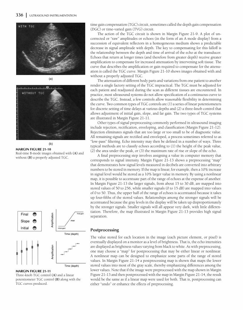
336 x ULTRASOUND INSTRUMENTATION
(a)
(b)
MARGIN FIGURE 21-10Real-time B-mode images obtained with (A) and
without (B) a properly adjusted TGC.
MARGIN FIGURE 21-11Three-knob TGC control (A) and a linear
potentiometer TGC control (B) along with the
TGC curves produced.
time gain compensation (TGC) circuit, sometimes called the depth gain compensation(DGC) or time-varied gain (TVG) circuit.
The action of the TGC circuit is shown in Margin Figure 21-9. A plot of un-corrected or “raw” amplitudes or echoes (in the form of an A mode display) from asuccession of equivalent reflectors in a homogeneous medium shows a predictabledecrease in signal amplitude with depth. The key to compensating for this falloff isthe relationship between the depth and time of arrival of the echo at the transducer.Echoes that return at longer times (and therefore from greater depth) receive greateramplification to compensate for increased attenuation by intervening soft tissue. Thecurve that describes the amplification or gain required to compensate for the attenu-ation is called the TGC curve. Margin Figure 21-10 shows images obtained with andwithout a properly adjusted TGC.
The attenuation of different body parts and variations from one patient to anotherrender a single factory setting of the TGC impractical. The TGC must be adjusted foreach patient and readjusted during the scan as different tissues are encountered. Inpractice, most ultrasound systems do not allow specification of a continuous curve todescribe the TGC. Instead, a few controls allow reasonable flexibility in determiningthe curve. Two common types of TGC controls are (1) a series of linear potentiometersfor discrete setting of time delays at various depths and (2) a three-knob control thatallows adjustment of initial gain, slope, and far gain. The two types of TGC systemsare illustrated in Margin Figure 21-11.
Other types of signal preprocessing commonly performed in ultrasound imaginginclude rejection, rectification, enveloping, and classification (Margin Figure 21-12).Rejection eliminates signals that are too large or too small to be of diagnostic value.All remaining signals are rectified and enveloped, a process sometimes referred to as“low-pass” filtering. Echo intensity may then be defined in a number of ways. Threetypical methods are to classify echoes according to (1) the height of the peak value,(2) the area under the peak, or (3) the maximum rate of rise or slope of the echo.
A final preprocessing step involves assigning a value in computer memory thatcorresponds to signal intensity. Margin Figure 21-13 shows a preprocessing “map”that demonstrates how signal levels measured in decibels are converted into arbitrarynumbers to be stored in memory. If the map is linear, for example, then a 10% increasein signal level would be stored as a 10% larger value in memory. By using a nonlinearmap, it is possible to accentuate part of the range of echoes at the expense of another.In Margin Figure 21-13 the larger signals, from about 15 to 30 dB, are mapped intostored values of 50 to 256, while smaller signals (0 to 15 dB) are mapped into valuesof 0 to 50. Thus, the upper half of the range of echoes is accentuated because it takesup four-fifths of the stored values. Relationships among the stronger signals will beaccentuated because the gray levels in the display will be taken up disproportionatelyby the stronger signals. Smaller signals will all appear very dark, with little differen-tiation. Therefore, the map illustrated in Margin Figure 21-13 provides high signalseparation.
Postprocessing
The value stored for each location in the image (each picture element, or pixel) iseventually displayed on a monitor as a level of brightness. That is, the echo intensitiesare displayed as brightness values varying from black to white. As with preprocessing,one may choose a “map” for postprocessing that may be either linear or nonlinear.A nonlinear map can be designed to emphasize some parts of the range of storedvalues. In Margin Figure 21-14 a postprocessing map is shown that maps the lowerstored values into most of the gray scale, thereby emphasizing differences among thelower values. Note that if the image were preprocessed with the map shown in MarginFigure 21-13 and then postprocessed with the map in Margin Figure 21-14, the resultwould be the same as if a linear map were used for both. That is, postprocessing caneither “undo” or enhance the effects of preprocessing.

DYNAMIC RANGE x 337
MARGIN FIGURE 21-12Signal preprocessing in ultrasound.
MARGIN FIGURE 21-13Preprocessing “map.” The graph shows how echo
signal levels are converted to stored values. This
particular example shows “high signal separation,”
with the upper half of the amplitude range taking
up the upper 4/5 of the stored values.
The terms “enveloping” and “low-pass
filtering” are used interchangeably in
signal processing. A low-pass filter
removes higher frequencies but allows
lower ones to pass through the circuit.
If a complex signal (one consisting of
varying amounts of many different
frequencies) is sent through a low-pass
filter, the resulting signal will look
something like the outline or envelope
of the original signal.
Other types of postprocessing features that may be present in an ultrasounddevice include zoom, region of interest, and digital filtering (see Chapter 10).
¥ DYNAMIC RANGE
The ratio of the largest to the smallest echoes processed by components of an ultra-sound device is known as the dynamic range of the device. In general, the dynamicrange decreases as signals pass through the imaging system (Margin Figure 21-15) be-cause operations such as TGC and rejection eliminate small and large signals. Echoesreturning from tissues can have dynamic ranges of 100 to 150 dB. The dynamic rangein decibels may be easily converted to a ratio of amplitudes or intensities.
Example 21-3
Find the amplitude and intensity ratios corresponding to a dynamic range of 100 dB.For amplitudes,
dB = 20 logA
A0
can be rewritten as
dB
20= log
A
A0
or
10dB/20=
A
A0
So, for 100 dB we have
105= 100,000 =
A
A0
The strongest echoes have 100,000 times the amplitude of the weakest echoes. Sim-ilarly, for intensity,
dB = 10 logI
I0
so that
10dB/10= 1010
= 10,000,000,000 =I
I0
The strongest echoes have 1010, or 10 billion, times the intensity of the weakestechoes.
Some of the dynamic range of echoes is caused by attenuation as the signalstraverse several centimeters of tissue. The TGC circuit amplifies the weak echoes thatarrive later, and rejection circuits eliminate low-amplitude noise. In this manner, thedynamic range is reduced, or “compressed,” to about 40 dB in the receiver/processor.This dynamic range may be retained in memory while a range of about 20 dB isdisplayed on the system monitor.
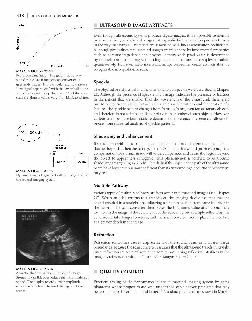
338 x ULTRASOUND INSTRUMENTATION
MARGIN FIGURE 21-14Postprocessing “map.” The graph shows how
stored values from memory are converted to
gray-scale values. This particular example shows
“low signal separation,” with the lower half of the
stored values taking up the lower 4/5 of the gray
scale (brightness values vary from black to white).
MARGIN FIGURE 21-15Dynamic range of signals at different stages of the
ultrasound imaging system.
MARGIN FIGURE 21-16Acoustic shadowing in an ultrasound image.
Stones in a gallbladder reduce the transmission of
sound. The display records lower amplitude
echoes or “shadows” beyond the region of the
stones.
¥ ULTRASOUND IMAGE ARTIFACTS
Even though ultrasound systems produce digital images, it is impossible to identifypixel values in typical clinical images with specific fundamental properties of tissuein the way that x-ray CT numbers are associated with linear attenuation coefficients.Although pixel values in ultrasound images are influenced by fundamental propertiessuch as acoustic impedance and physical density, each pixel value is determinedby interrelationships among surrounding materials that are too complex to unfoldquantitatively. However, these interrelationships sometimes create artifacts that arerecognizable in a qualitative sense.
Speckle
The physical principles behind the phenomenon of speckle were described in Chapter20. Although the presence of speckle in an image indicates the presence of featuresin the patient that are smaller than the wavelength of the ultrasound, there is noone-to-one correspondence between a dot in a speckle pattern and the location of afeature. The speckle pattern changes from frame to frame, even for stationary objects,and therefore is not a simple indicator of even the number of such objects. However,various attempts have been made to determine the presence or absence of disease inorgans from statistical analysis of speckle patterns.1
Shadowing and Enhancement
If some object within the patient has a larger attenuation coefficient than the materialthat lies beyond it, then the settings of the TGC circuit that would provide appropriatecompensation for normal tissue will undercompensate and cause the region beyondthe object to appear less echogenic. This phenomenon is referred to as acousticshadowing (Margin Figure 21-16). Similarly, if the object in the path of the ultrasoundbeam has a lower attenuation coefficient than its surroundings, acoustic enhancementmay result.
Multiple Pathway
Various types of multiple-pathway artifacts occur in ultrasound images (see Chapter20). When an echo returns to a transducer, the imaging device assumes that thesound traveled in a straight line following a single reflection from some interface inthe patient. The scan converter then places the brightness value at an appropriatelocation in the image. If the actual path of the echo involved multiple reflections, theecho would take longer to return, and the scan converter would place the interfaceat a greater depth in the image.
Refraction
Refraction sometimes causes displacement of the sound beam as it crosses tissueboundaries. Because the scan converter assumes that the ultrasound travels in straightlines, refraction causes displacement errors in positioning reflective interfaces in theimage. A refraction artifact is illustrated in Margin Figure 21-17.
¥ QUALITY CONTROL
Frequent testing of the performance of the ultrasound imaging system by usingphantoms whose properties are well understood can uncover problems that maybe too subtle to discern in clinical images.2 Standard phantoms are shown in Margin
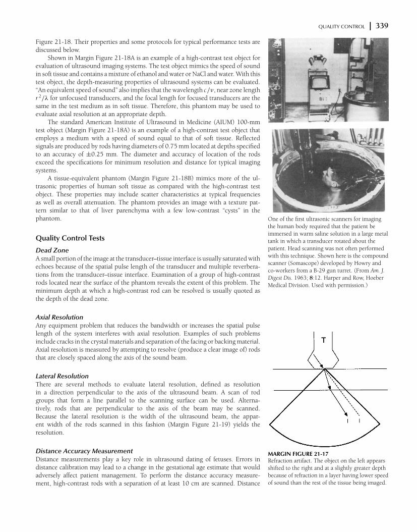
QUALITY CONTROL x 339
MARGIN FIGURE 21-17Refraction artifact. The object on the left appears
shifted to the right and at a slightly greater depth
because of refraction in a layer having lower speed
of sound than the rest of the tissue being imaged.
One of the first ultrasonic scanners for imaging
the human body required that the patient be
immersed in warm saline solution in a large metal
tank in which a transducer rotated about the
patient. Head scanning was not often performed
with this technique. Shown here is the compound
scanner (Somascope) developed by Howry and
co-workers from a B-29 gun turret. (From Am. J.
Digest Dis. 1963; 8:12. Harper and Row, Hoeber
Medical Division. Used with permission.)
Figure 21-18. Their properties and some protocols for typical performance tests arediscussed below.
Shown in Margin Figure 21-18A is an example of a high-contrast test object forevaluation of ultrasound imaging systems. The test object mimics the speed of soundin soft tissue and contains a mixture of ethanol and water or NaCl and water. With thistest object, the depth-measuring properties of ultrasound systems can be evaluated.“An equivalent speed of sound” also implies that the wavelength c/ν, near zone lengthr 2/λ for unfocused transducers, and the focal length for focused transducers are thesame in the test medium as in soft tissue. Therefore, this phantom may be used toevaluate axial resolution at an appropriate depth.
The standard American Institute of Ultrasound in Medicine (AIUM) 100-mmtest object (Margin Figure 21-18A) is an example of a high-contrast test object thatemploys a medium with a speed of sound equal to that of soft tissue. Reflectedsignals are produced by rods having diameters of 0.75 mm located at depths specifiedto an accuracy of ±0.25 mm. The diameter and accuracy of location of the rodsexceed the specifications for minimum resolution and distance for typical imagingsystems.
A tissue-equivalent phantom (Margin Figure 21-18B) mimics more of the ul-trasonic properties of human soft tissue as compared with the high-contrast testobject. These properties may include scatter characteristics at typical frequenciesas well as overall attenuation. The phantom provides an image with a texture pat-tern similar to that of liver parenchyma with a few low-contrast “cysts” in thephantom.
Quality Control Tests
Dead ZoneA small portion of the image at the transducer–tissue interface is usually saturated withechoes because of the spatial pulse length of the transducer and multiple reverbera-tions from the transducer–tissue interface. Examination of a group of high-contrastrods located near the surface of the phantom reveals the extent of this problem. Theminimum depth at which a high-contrast rod can be resolved is usually quoted asthe depth of the dead zone.
Axial ResolutionAny equipment problem that reduces the bandwidth or increases the spatial pulselength of the system interferes with axial resolution. Examples of such problemsinclude cracks in the crystal materials and separation of the facing or backing material.Axial resolution is measured by attempting to resolve (produce a clear image of) rodsthat are closely spaced along the axis of the sound beam.
Lateral ResolutionThere are several methods to evaluate lateral resolution, defined as resolutionin a direction perpendicular to the axis of the ultrasound beam. A scan of rodgroups that form a line parallel to the scanning surface can be used. Alterna-tively, rods that are perpendicular to the axis of the beam may be scanned.Because the lateral resolution is the width of the ultrasound beam, the appar-ent width of the rods scanned in this fashion (Margin Figure 21-19) yields theresolution.
Distance Accuracy MeasurementDistance measurements play a key role in ultrasound dating of fetuses. Errors indistance calibration may lead to a change in the gestational age estimate that wouldadversely affect patient management. To perform the distance accuracy measure-ment, high-contrast rods with a separation of at least 10 cm are scanned. Distance
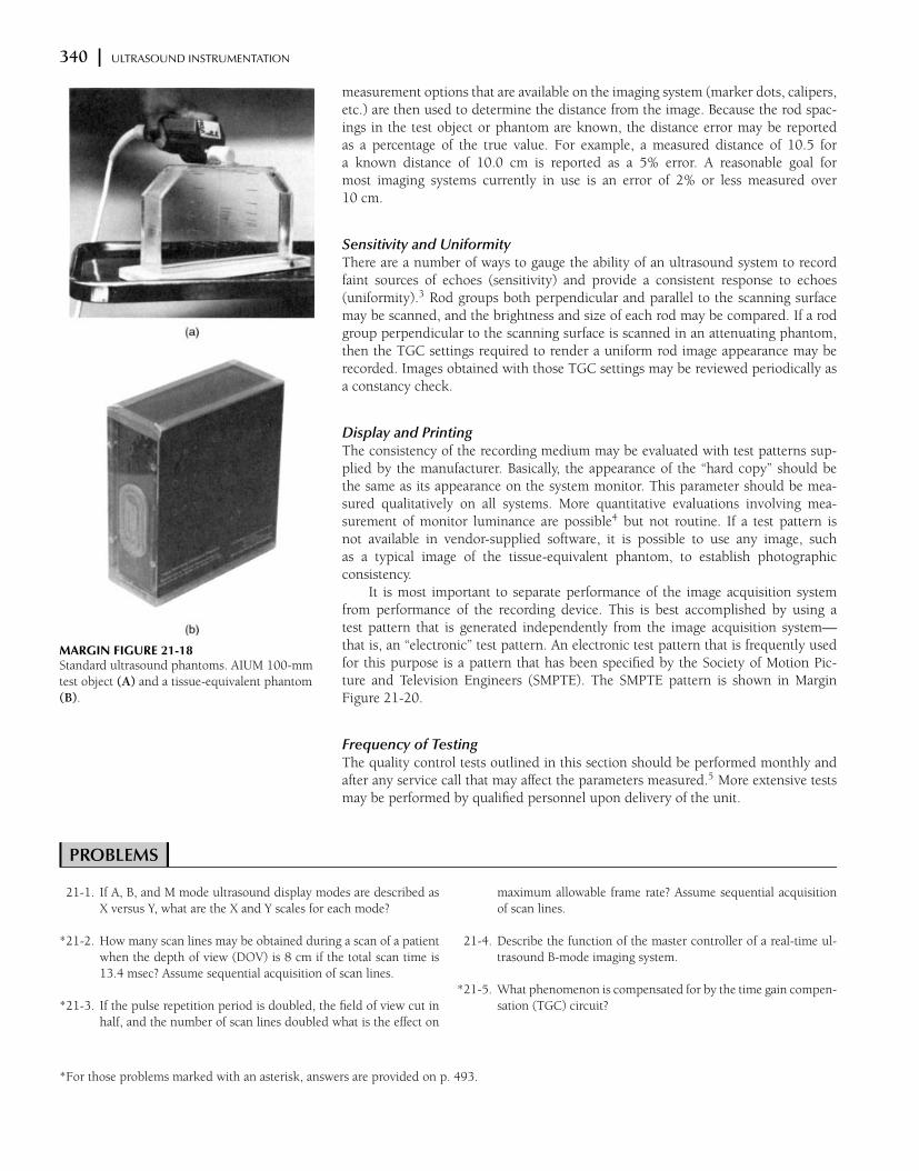
340 x ULTRASOUND INSTRUMENTATION
MARGIN FIGURE 21-18Standard ultrasound phantoms. AIUM 100-mm
test object (A) and a tissue-equivalent phantom
(B).
measurement options that are available on the imaging system (marker dots, calipers,etc.) are then used to determine the distance from the image. Because the rod spac-ings in the test object or phantom are known, the distance error may be reportedas a percentage of the true value. For example, a measured distance of 10.5 fora known distance of 10.0 cm is reported as a 5% error. A reasonable goal formost imaging systems currently in use is an error of 2% or less measured over10 cm.
Sensitivity and UniformityThere are a number of ways to gauge the ability of an ultrasound system to recordfaint sources of echoes (sensitivity) and provide a consistent response to echoes(uniformity).3 Rod groups both perpendicular and parallel to the scanning surfacemay be scanned, and the brightness and size of each rod may be compared. If a rodgroup perpendicular to the scanning surface is scanned in an attenuating phantom,then the TGC settings required to render a uniform rod image appearance may berecorded. Images obtained with those TGC settings may be reviewed periodically asa constancy check.
Display and PrintingThe consistency of the recording medium may be evaluated with test patterns sup-plied by the manufacturer. Basically, the appearance of the “hard copy” should bethe same as its appearance on the system monitor. This parameter should be mea-sured qualitatively on all systems. More quantitative evaluations involving mea-surement of monitor luminance are possible4 but not routine. If a test pattern isnot available in vendor-supplied software, it is possible to use any image, suchas a typical image of the tissue-equivalent phantom, to establish photographicconsistency.
It is most important to separate performance of the image acquisition systemfrom performance of the recording device. This is best accomplished by using atest pattern that is generated independently from the image acquisition system—that is, an “electronic” test pattern. An electronic test pattern that is frequently usedfor this purpose is a pattern that has been specified by the Society of Motion Pic-ture and Television Engineers (SMPTE). The SMPTE pattern is shown in MarginFigure 21-20.
Frequency of TestingThe quality control tests outlined in this section should be performed monthly andafter any service call that may affect the parameters measured.5 More extensive testsmay be performed by qualified personnel upon delivery of the unit.
x PROBLEMS x21-1. If A, B, and M mode ultrasound display modes are described as
X versus Y, what are the X and Y scales for each mode?
*21-2. How many scan lines may be obtained during a scan of a patient
when the depth of view (DOV) is 8 cm if the total scan time is
13.4 msec? Assume sequential acquisition of scan lines.
*21-3. If the pulse repetition period is doubled, the field of view cut in
half, and the number of scan lines doubled what is the effect on
maximum allowable frame rate? Assume sequential acquisition
of scan lines.
21-4. Describe the function of the master controller of a real-time ul-
trasound B-mode imaging system.
*21-5. What phenomenon is compensated for by the time gain compen-
sation (TGC) circuit?
*For those problems marked with an asterisk, answers are provided on p. 493.

REFERENCES x 341
(a) (b)
MARGIN FIGURE 21-19Scan of a rod group in an ultrasound phantom
demonstrates beam width (lateral resolution).
MARGIN FIGURE 21-20The test pattern promulgated by the Society of
Motion Pictures and Television Engineers
(SMPTE), known colloquially as the “sımte
pattern.” This pattern, which tests image quality
parameters such as high and low contrast
resolution, distortion, and linearity, may be used
as an electronic data file to test the fidelity of
displays, hard-copy devices, or storage and
transmission systems. (ref: Society of Motion
Pictures and Television Engineers (SMPTE).
Specifications for Medical Diagnostic Imaging Test
Pattern for Television Monitors and Hard-Copy
Recording Cameras. Recommended Practice
RP 133-1986. SMPTE J. 1986; 95:693–695.)
¥ SUMMARY
r Display modes includer Amplituder Brightnessr Motion
r Frame rate is inversely proportional to depth of view, number of scan lines, andpulse repetition frequency.
r The main components of an ultrasound imaging system arer Transducerr Transmit/receive switchr Transmitterr Receiver/processorr Master controllerr Memoryr Displayr Storage
r The time gain compensation system varies the amplification of return signalsfrom each scan line in a variable manner as a function of time after the sentpulse.
r Preprocessing steps includer Rectificationr Pulse height rejectionr Enveloping (low-pass filtering)r Classification (e.g., differential, peak, area, alone or some combination)
r In preprocessing, echo signals are assigned to stored values according to accord-ing to a functional form or curve.
r In postprocessing, stored values are assigned to the gray scale according to afunctional form or curve.
r Artifacts includer Speckler Acoustic shadowingr Multiple pathwayr Refraction
r Ultrasound quality control tests includer Dead zoner Axial resolutionr Lateral resolutionr Distance accuracyr Sensitivity and uniformity
x REFERENCES x1. Allison, J. W., et al. Understanding the process of quantitative ultrasonic tissue
characterization. Radiographics 1994; 14(5):1099–1108.
2. General Medical Physics Committee Ultrasound Task Group. Pulse Echo Ultra-
sound Imaging Systems: Performance Tests and Criteria. Medical Physics Publish-
ing, Madison, WI, 1980.
3. Smith, S. W., and Lopez, L. A contrast-detail analysis of diagnostic ultrasound
imaging. Med. Phys. 1982; 9:4–12.
4. Ritenour, E. R., Sahu, S. N., Rossi, R. P., et al. Quantitative methods for hardcopy
device adjustment, Paper 766-67. Presented at the Society of Photo-Optical
Instrumentation Engineers, Medicine/Pattern Recognition, Newport Beach,
CA, 1987.
5. Goodsit, M. M., et al. Real-time B-mode ultrasound quality control test pro-
cedures, Report of AAPM Ultrasound Task Group No 1, Medical Phys. 1998;
25(8):1385–1406.
C H A P T E R
22DOPPLER EFFECT
OBJECTIVES 344
ORIGIN OF DOPPLER SHIFT 344
Pulsed Doppler 348
Spectral Analysis 349
Frequency Spectrum 349
Spectral Trace 349
Color Mapping 350
Quantitative Use of Doppler 350
LIMITATIONS OF DOPPLER SYSTEMS 351
Pulse Repetition Frequency 351
Spectral Broadening 352
PROBLEMS 352
SUMMARY 352
REFERENCES 353
Medical Imaging Physics, Fourth Edition, by William R. Hendee and E. Russell RitenourISBN: 0-471-38226-4 Copyright C© 2002 Wiley-Liss, Inc. 343

344 x DOPPLER EFFECT
d sl
dsl
(b)
(a)
MARGIN FIGURE 22-1Principles of Doppler ultrasound. A: Source
moving toward a stationary detector d. B: Source
moving away from a stationary detector d.
¥ OBJECTIVES
After completing this chapter, the reader should be able to:
r Write the Doppler equation and use it to calculate the Doppler shift.r Describe the effect of Doppler angle upon frequency shift and describe how error
in estimation of the angle influences the accuracy of velocity estimation.r Determine volumetric flow from average velocity and vessel cross-sectional area.r Name the main components of a Doppler ultrasound imager.r Calculate range gate size and depth from timing information.r Describe the differences between information obtained from pulsed-wave versus
continuous-wave Doppler.r Describe the main features of a frequency spectrum and describe how it is used
in constructing the Doppler spectral trace.r Describe how color is assigned in color Doppler.r Discuss some reasons for spectral broadening.
Ultrasound is used not only for display of static patient anatomy but also for identi-fication of moving structures in the body. Approaches to the identification of movingstructures include real-time pulse-echo imaging, motion mode (M-mode) display ofreflected ultrasound pulses, and the Doppler-shift method. Discussed in this chapterare the basic principles of the Doppler-shift method. The Doppler method has anumber of applications in clinical medicine, including detection of fetal heartbeat,detection of air emboli, blood pressure monitoring, detection and characterization ofblood flow, and localization of blood vessel occlusions.1,2
When an emergency vehicle with its
siren on passes someone on the street, a
shift in frequency of one octave on the
chromatic musical scale corresponds to
a velocity difference between the siren
and the listener of 40 miles per hour,
two octaves corresponds to 80 miles
per hour, and so on.
¥ ORIGIN OF DOPPLER SHIFT
When there is relative motion between a source and a detector of ultrasound, thefrequency of the detected ultrasound differs from that emitted by the source. Theshift in frequency is illustrated in Margin Figure 22-1. In Margin Figure 22-1A,an ultrasound source is moving with velocity vs toward the detector. After time tfollowing the production of any particular wave front, the distance between thewave front and the source is (c − vs )t , where c is the velocity of ultrasound in themedium. The wavelength λ of the ultrasound in the direction of motion is shortenedto
λ =c − vs
ν0
where ν0 is the frequency of ultrasound from the source. With the shortenedwavelength, the ultrasound reaches the detector with an increased frequency ν:
ν =c
λ=
c
(c − vs )/ν0
= ν0
(
c
c − vs
)
That is, the frequency of the detected ultrasound shifts to a higher value when theultrasound source is moving toward the detector. The shift in frequency 1ν is
1ν = ν − ν0 = ν0
(
c
c − vs
)
− ν0
= ν0
(
vs
c − vs
)
ORIGIN OF DOPPLER SHIFT x 345
If the velocity c of ultrasound in the medium is much greater than the velocity vs ofthe ultrasound source, then c − vs ' c and
1ν = ν0
(vs
c
)
A similar expression is applicable to the case in which the ultrasound source isstationary and the detector is moving toward the source with velocity vd . In this casethe Doppler-shift frequency is approximately
1ν = ν0
(vd
c
)
where c >> vd .If the ultrasound source is moving away from the detector (Margin Figure 22-1B),
then the distance between the source and a wavefront is ct + vs t = (c + vs )t , wheret is the time elapsed since the production of the wavefront. The wavelength λ of theultrasound is
λ =c + vs
ν0
and the apparent frequency ν is
ν =c
λ
=c
(c + vs )/ν0
= ν0
(
c
c + vs
)
That is, the frequency shifts to a lower value when the ultrasound source is movingaway from the detector. The shift in frequency 1ν is
1ν = ν − ν0 = ν0
(
c
c + vs
)
− ν0
= ν0
(
−vs
c + vs
)
where the negative sign implies a reduction in frequency. If the velocity c of ultrasoundis much greater than the velocity vs of the source, c + vs ' c , and 1ν = ν0(−vs /c).A similar expression is applicable to the case where the ultrasound source is stationaryand the detector is moving away from the source with velocity vd :
1ν = ν0
(
−vd
c
)
when c >> vd .If the source and detector are at the same location and ultrasound is reflected
from an object moving toward the location with velocity v, the object acts first as amoving detector as it receives the ultrasound signal and then as a moving source as itreflects the signal. As a result, the ultrasound signal received by the detector exhibitsa frequency shift (when c >> v )
1ν = 2ν0
v
c
Similarly, for an object moving away from the source and detector, the shift in fre-quency 1ν is
1ν = 2ν0
(
−v
c
)
where the negative sign indicates that the frequency of the detected ultrasound islower than that emitted by the source.
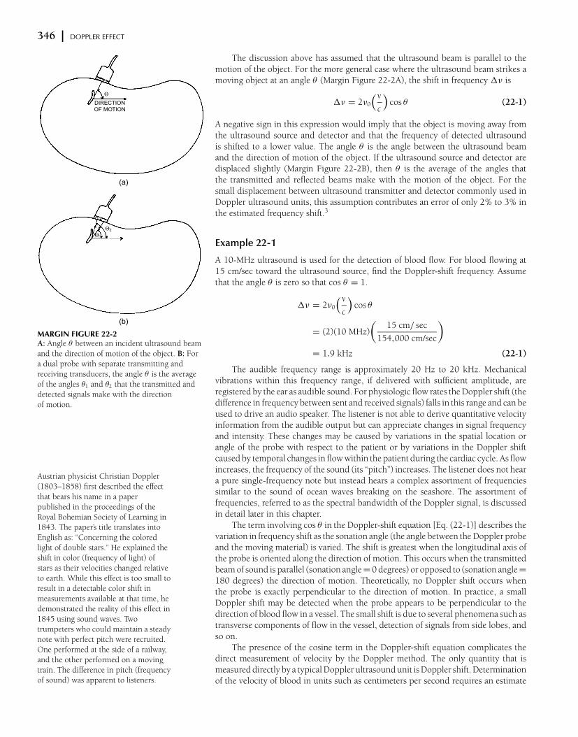
346 x DOPPLER EFFECT
DIRECTIONOF MOTION
(a)
(b)
Θ
Θ2
Θ1
MARGIN FIGURE 22-2A: Angle θ between an incident ultrasound beam
and the direction of motion of the object. B: For
a dual probe with separate transmitting and
receiving transducers, the angle θ is the average
of the angles θ1 and θ2 that the transmitted and
detected signals make with the direction
of motion.
The discussion above has assumed that the ultrasound beam is parallel to themotion of the object. For the more general case where the ultrasound beam strikes amoving object at an angle θ (Margin Figure 22-2A), the shift in frequency 1ν is
1ν = 2ν0
(v
c
)
cos θ (22-1)
A negative sign in this expression would imply that the object is moving away fromthe ultrasound source and detector and that the frequency of detected ultrasoundis shifted to a lower value. The angle θ is the angle between the ultrasound beamand the direction of motion of the object. If the ultrasound source and detector aredisplaced slightly (Margin Figure 22-2B), then θ is the average of the angles thatthe transmitted and reflected beams make with the motion of the object. For thesmall displacement between ultrasound transmitter and detector commonly used inDoppler ultrasound units, this assumption contributes an error of only 2% to 3% inthe estimated frequency shift.3
Example 22-1
A 10-MHz ultrasound is used for the detection of blood flow. For blood flowing at15 cm/sec toward the ultrasound source, find the Doppler-shift frequency. Assumethat the angle θ is zero so that cos θ = 1.
1ν = 2ν0
(v
c
)
cos θ
= (2)(10 MHz)
(
15 cm/ sec
154,000 cm/sec
)
= 1.9 kHz (22-1)
Austrian physicist Christian Doppler
(1803–1858) first described the effect
that bears his name in a paper
published in the proceedings of the
Royal Bohemian Society of Learning in
1843. The paper’s title translates into
English as: “Concerning the colored
light of double stars.” He explained the
shift in color (frequency of light) of
stars as their velocities changed relative
to earth. While this effect is too small to
result in a detectable color shift in
measurements available at that time, he
demonstrated the reality of this effect in
1845 using sound waves. Two
trumpeters who could maintain a steady
note with perfect pitch were recruited.
One performed at the side of a railway,
and the other performed on a moving
train. The difference in pitch (frequency
of sound) was apparent to listeners.
The audible frequency range is approximately 20 Hz to 20 kHz. Mechanicalvibrations within this frequency range, if delivered with sufficient amplitude, areregistered by the ear as audible sound. For physiologic flow rates the Doppler shift (thedifference in frequency between sent and received signals) falls in this range and can beused to drive an audio speaker. The listener is not able to derive quantitative velocityinformation from the audible output but can appreciate changes in signal frequencyand intensity. These changes may be caused by variations in the spatial location orangle of the probe with respect to the patient or by variations in the Doppler shiftcaused by temporal changes in flow within the patient during the cardiac cycle. As flowincreases, the frequency of the sound (its “pitch”) increases. The listener does not heara pure single-frequency note but instead hears a complex assortment of frequenciessimilar to the sound of ocean waves breaking on the seashore. The assortment offrequencies, referred to as the spectral bandwidth of the Doppler signal, is discussedin detail later in this chapter.
The term involving cos θ in the Doppler-shift equation [Eq. (22-1)] describes thevariation in frequency shift as the sonation angle (the angle between the Doppler probeand the moving material) is varied. The shift is greatest when the longitudinal axis ofthe probe is oriented along the direction of motion. This occurs when the transmittedbeam of sound is parallel (sonation angle = 0 degrees) or opposed to (sonation angle =
180 degrees) the direction of motion. Theoretically, no Doppler shift occurs whenthe probe is exactly perpendicular to the direction of motion. In practice, a smallDoppler shift may be detected when the probe appears to be perpendicular to thedirection of blood flow in a vessel. The small shift is due to several phenomena such astransverse components of flow in the vessel, detection of signals from side lobes, andso on.
The presence of the cosine term in the Doppler-shift equation complicates thedirect measurement of velocity by the Doppler method. The only quantity that ismeasured directly by a typical Doppler ultrasound unit is Doppler shift. Determinationof the velocity of blood in units such as centimeters per second requires an estimate
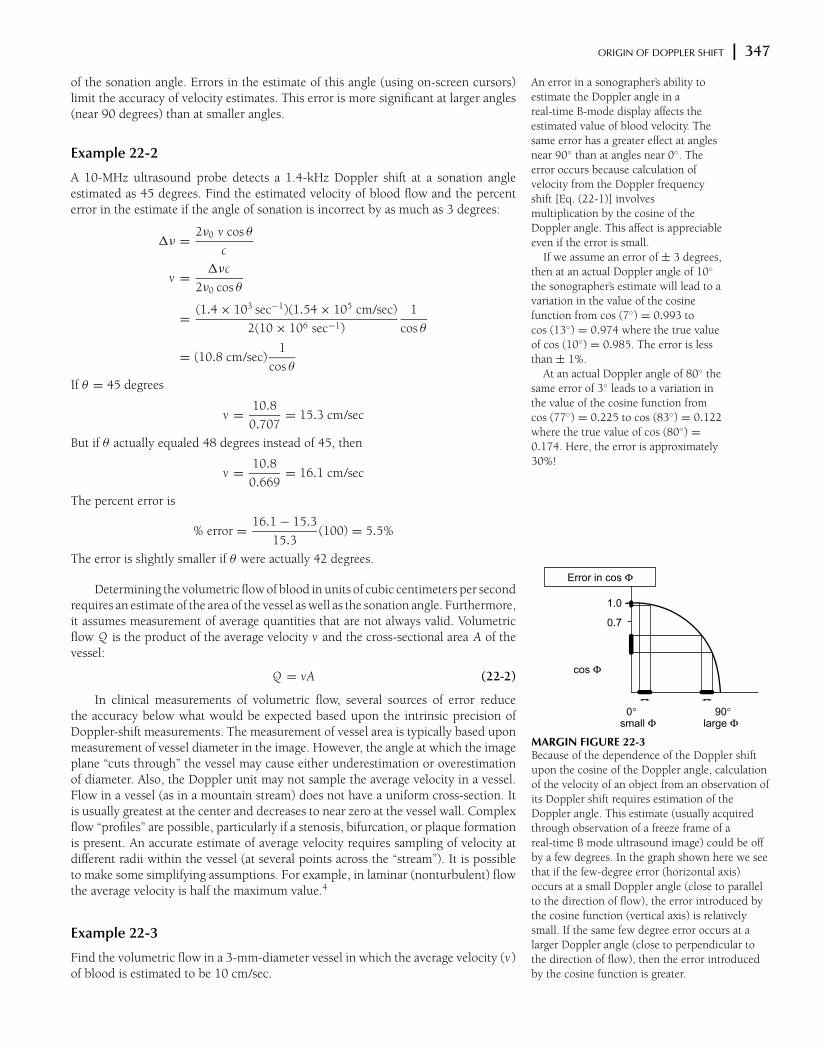
ORIGIN OF DOPPLER SHIFT x 347
Error in cos Φ
cos Φ
small Φ large Φ
1.0
0.7
0° 90°
MARGIN FIGURE 22-3Because of the dependence of the Doppler shift
upon the cosine of the Doppler angle, calculation
of the velocity of an object from an observation of
its Doppler shift requires estimation of the
Doppler angle. This estimate (usually acquired
through observation of a freeze frame of a
real-time B mode ultrasound image) could be off
by a few degrees. In the graph shown here we see
that if the few-degree error (horizontal axis)
occurs at a small Doppler angle (close to parallel
to the direction of flow), the error introduced by
the cosine function (vertical axis) is relatively
small. If the same few degree error occurs at a
larger Doppler angle (close to perpendicular to
the direction of flow), then the error introduced
by the cosine function is greater.
of the sonation angle. Errors in the estimate of this angle (using on-screen cursors)limit the accuracy of velocity estimates. This error is more significant at larger angles(near 90 degrees) than at smaller angles.
Example 22-2
A 10-MHz ultrasound probe detects a 1.4-kHz Doppler shift at a sonation angleestimated as 45 degrees. Find the estimated velocity of blood flow and the percenterror in the estimate if the angle of sonation is incorrect by as much as 3 degrees:
1ν =2ν0 v cos θ
c
v =1νc
2ν0 cos θ
=(1.4 × 10³ sec−1)(1.54 × 105 cm/sec)
2(10 × 106 sec−1)
1
cos θ
= (10.8 cm/sec)1
cos θ
If θ = 45 degrees
v =10.8
0.707= 15.3 cm/sec
But if θ actually equaled 48 degrees instead of 45, then
v =10.8
0.669= 16.1 cm/sec
The percent error is
% error =16.1 − 15.3
15.3(100) = 5.5%
The error is slightly smaller if θ were actually 42 degrees.
An error in a sonographer’s ability to
estimate the Doppler angle in a
real-time B-mode display affects the
estimated value of blood velocity. The
same error has a greater effect at angles
near 90◦ than at angles near 0◦. The
error occurs because calculation of
velocity from the Doppler frequency
shift [Eq. (22-1)] involves
multiplication by the cosine of the
Doppler angle. This affect is appreciable
even if the error is small.
If we assume an error of ± 3 degrees,
then at an actual Doppler angle of 10◦
the sonographer’s estimate will lead to a
variation in the value of the cosine
function from cos (7◦) = 0.993 to
cos (13◦) = 0.974 where the true value
of cos (10◦) = 0.985. The error is less
than ± 1%.
At an actual Doppler angle of 80◦ the
same error of 3◦ leads to a variation in
the value of the cosine function from
cos (77◦) = 0.225 to cos (83◦) = 0.122
where the true value of cos (80◦) =
0.174. Here, the error is approximately
30%!
Determining the volumetric flow of blood in units of cubic centimeters per secondrequires an estimate of the area of the vessel as well as the sonation angle. Furthermore,it assumes measurement of average quantities that are not always valid. Volumetricflow Q is the product of the average velocity v and the cross-sectional area A of thevessel:
Q = vA (22-2)
In clinical measurements of volumetric flow, several sources of error reducethe accuracy below what would be expected based upon the intrinsic precision ofDoppler-shift measurements. The measurement of vessel area is typically based uponmeasurement of vessel diameter in the image. However, the angle at which the imageplane “cuts through” the vessel may cause either underestimation or overestimationof diameter. Also, the Doppler unit may not sample the average velocity in a vessel.Flow in a vessel (as in a mountain stream) does not have a uniform cross-section. Itis usually greatest at the center and decreases to near zero at the vessel wall. Complexflow “profiles” are possible, particularly if a stenosis, bifurcation, or plaque formationis present. An accurate estimate of average velocity requires sampling of velocity atdifferent radii within the vessel (at several points across the “stream”). It is possibleto make some simplifying assumptions. For example, in laminar (nonturbulent) flowthe average velocity is half the maximum value.4
Example 22-3
Find the volumetric flow in a 3-mm-diameter vessel in which the average velocity (v )of blood is estimated to be 10 cm/sec.
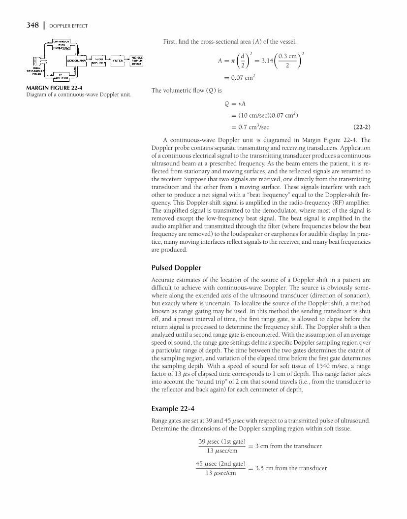
348 x DOPPLER EFFECT
MARGIN FIGURE 22-4Diagram of a continuous-wave Doppler unit.
First, find the cross-sectional area (A) of the vessel.
A = π
(
d
2
)2
= 3.14
(
0.3 cm
2
)2
= 0.07 cm2
The volumetric flow (Q ) is
Q = vA
= (10 cm/sec)(0.07 cm2)
= 0.7 cm3/sec (22-2)
A continuous-wave Doppler unit is diagramed in Margin Figure 22-4. TheDoppler probe contains separate transmitting and receiving transducers. Applicationof a continuous electrical signal to the transmitting transducer produces a continuousultrasound beam at a prescribed frequency. As the beam enters the patient, it is re-flected from stationary and moving surfaces, and the reflected signals are returned tothe receiver. Suppose that two signals are received, one directly from the transmittingtransducer and the other from a moving surface. These signals interfere with eachother to produce a net signal with a “beat frequency” equal to the Doppler-shift fre-quency. This Doppler-shift signal is amplified in the radio-frequency (RF) amplifier.The amplified signal is transmitted to the demodulator, where most of the signal isremoved except the low-frequency beat signal. The beat signal is amplified in theaudio amplifier and transmitted through the filter (where frequencies below the beatfrequency are removed) to the loudspeaker or earphones for audible display. In prac-tice, many moving interfaces reflect signals to the receiver, and many beat frequenciesare produced.
Pulsed Doppler
Accurate estimates of the location of the source of a Doppler shift in a patient aredifficult to achieve with continuous-wave Doppler. The source is obviously some-where along the extended axis of the ultrasound transducer (direction of sonation),but exactly where is uncertain. To localize the source of the Doppler shift, a methodknown as range gating may be used. In this method the sending transducer is shutoff, and a preset interval of time, the first range gate, is allowed to elapse before thereturn signal is processed to determine the frequency shift. The Doppler shift is thenanalyzed until a second range gate is encountered. With the assumption of an averagespeed of sound, the range gate settings define a specific Doppler sampling region overa particular range of depth. The time between the two gates determines the extent ofthe sampling region, and variation of the elapsed time before the first gate determinesthe sampling depth. With a speed of sound for soft tissue of 1540 m/sec, a rangefactor of 13 µs of elapsed time corresponds to 1 cm of depth. This range factor takesinto account the “round trip” of 2 cm that sound travels (i.e., from the transducer tothe reflector and back again) for each centimeter of depth.
Example 22-4
Range gates are set at 39 and 45 µsec with respect to a transmitted pulse of ultrasound.Determine the dimensions of the Doppler sampling region within soft tissue.
39 µsec (1st gate)
13 µsec/cm= 3 cm from the transducer
45 µsec (2nd gate)
13 µsec/cm= 3.5 cm from the transducer

ORIGIN OF DOPPLER SHIFT x 349
MARGIN FIGURE 22-5Diagram of a pulsed Doppler unit.
MARGIN FIGURE 22-6Doppler-shift frequency spectrum showing the
relative contribution of frequencies to the Doppler
shift during a brief interval of time.
The Doppler sampling region begins at a depth of 3 cm and extends to a depth of3.5 cm. We could state that there is a 0.5-cm sampling region centered at a depth of3.25 cm. The width of the sampling region is roughly equal to the ultrasound beamwidth at that depth.
In Doppler systems that are used in conjunction with imaging, the positionof the sampling volume is usually indicated by cursors positioned on the display.The ultrasound computer performs the electronic equivalent of the calculations inExample 22-4 to determine where the cursors should appear on the image.
Range gating requires that the ultrasound be started and stopped (i.e., pulsed)during the signal acquisition process so that the time to echo may be determinedunambiguously. The use of pulsed Doppler not only allows range gating but alsopermits imaging pulses to be interspersed with Doppler pulses. Thus a real-timeB-mode image of the patient may be obtained from every other pulse. In continuous-wave Doppler there is, by definition, no time in which to send imaging pulses, becausethere is no gap in the Doppler process.
A simplified diagram of a pulsed Doppler ultrasound system is shown in MarginFigure 22-5. The main differences between the pulsed Doppler system in this illustra-tion and the continuous-wave system of Margin Figure 22-4 are that the pulsed systemincludes range gates and a transmit–receive switch similar to that in B-mode systems.Units that intersperse Doppler and imaging pulses incorporate components found instandard B-mode systems with both Doppler and B-mode components connected tothe voltage generator or oscillator so that the sending of Doppler and imaging pulsescan be coordinated.
There are techniques for determining
velocity in ultrasound images that do
not use the Doppler frequency shift
effect. In “time domain” analysis, the
return signals along scan lines are
compared in a process known as
“autocorrelation analysis” to determine
if a signal anywhere in the image in one
frame appears at a different location in
another frame. This information is then
color-coded using any of the techniques
that are used in color Doppler.
Spectral Analysis
The Doppler-shift signal contains a wealth of information. One of the fundamentalchallenges of Doppler ultrasound is to display that information in a useful fashion.Doppler shift in a blood vessel is produced by the flow of red blood cells (RBCs).However, within a single vessel there is an assortment (distribution) of RBC velocities.Also, the velocity of any given cell varies with time according to the cardiac cycle. Threemethods for visual display of information are discussed here: frequency spectrum,spectral trace, and color mapping.
Frequency Spectrum
A frequency spectrum (Margin Figure 22-6) is a histogram in which the horizontal axisdepicts Doppler-shift frequency and the vertical axis shows the relative contribution ofeach frequency to the observed Doppler shift. For simplicity, the frequency spectrumcan be thought of as a histogram of the relative distribution of RBC velocities in a bloodvessel. The peak of the spectrum shows the Doppler shift associated with the greatestnumber of RBCs. The frequency spectrum is a “snapshot” depicting the conditions offlow in the sampling volume at a particular moment in time. To determine temporalvariations, a display such as the flow plot is required.
Spectral Trace
A spectral trace (Margin Figure 22-7) is a graph of frequency versus time that depictsthe manner in which the value of Doppler shift varies with time. The value indictedmay be the average, minimum, or maximum Doppler shift, and a distribution of valuesmay be indicated by a vertical bar. The spectral trace may be displayed as a Doppler-shift frequency trace or as a velocity trace. The velocity trace is obtained by usingthe center frequency of the probe and the sonation angle measured by the operatorto convert the Doppler-shift frequency scale a velocity scale (see Example 22-2).Audible sound may be broadcast by speakers as the trace is displayed in real time

350 x DOPPLER EFFECT
MARGIN FIGURE 22-7Doppler spectral trace showing Doppler shift as a
function of time. The distribution of Doppler
shifts at any given time is the vertical “thickness”
of the trace. Thus, the Doppler spectral trace
shows changes in the frequency spectrum
over time.
by using a “moving pen” or “strip chart” type of display. Cardiac information suchas electrocardiographic (ECG) tracings may also be displayed to allow the viewer tocoordinate features in the spectral trace with timing of the cardiac cycle. Some systemsalso allow the user to display a frequency spectrum for a selected moment of timeduring display of the spectral trace.
Color Mapping
Both frequency spectra and spectral traces may be displayed along with B-modeimages by dividing the display screen into separate “windows” (compartments).Cursors on the image indicate the Doppler sampling volume. It is possible to in-dicate flow directly within the image by color-coding the pixels. In color mappingor color-flow Doppler, pixels in the B-mode image that correspond to regions inthe patient where flow is present are assigned hues (colors such as red, blue, green)according to an arbitrary color scale. For example, red may indicate a large posi-tive Doppler shift, orange a smaller positive shift, yellow a small negative shift, andso on.
Alternatively, the color scale may involve only two hues. One of the most com-mon two-hue systems uses red for a positive Doppler shift and blue for a negativeDoppler shift. The magnitude of the Doppler shift is encoded by the “saturation”of the color. Saturation is the degree to which the hue is present. A totally un-saturated color is white. It emits a broad distribution of all frequencies of visiblelight. Higher saturation implies that more of the frequencies in the spectrum areof a single frequency, interpreted by our retina as a purer color. The saturation en-coding in color Doppler is usually arranged such that a greater shift (higher velo-city either toward or away from the transducer) is encoded as a less saturated hue.For example, a small positive Doppler shift would be indicated by a dark red,whereas a larger positive Doppler shift would be indicated by a lighter, less satura-ted red.
Whatever color scale is used in color Doppler, it is desirable to avoid color-codingthe very slow velocities of tissues that occur in the patient as pliable tissues are pushedby the transducer and as the transducer itself is moved. Detection of such motionsis not usually the purpose of the exam. Thus, most color scales do not assign colorto very small Doppler shifts and display a black band at the center of the color scaleindicator. The width of the black band may be changed by the operator to vary therange of velocities that will be color-coded.
The large variety of color scales that could be used in color Doppler, as well asthe variation in perception of color from one individual to another, is an intriguingproblem for optimization of visual perception.
In color Doppler, the most commonly
used color scale codes flow away from
the transducer as blue and flow toward
the transducer as red. When such a
“blue away red toward” (BART) display
is used, it is sometimes necessary to
remind observers that the colors are not
necessarily correlated with the
oxygenation (venous or arterial) status
of the blood.
Quantitative Use of Doppler
Various attempts have been made to correlate information obtained from Dopplerdisplays, particularly spectral traces, with pathology. Simple measures such as thepeak systolic or end-diastolic average velocities are probably too crude to differentiatenormal and disease states, in part because of the wide range of normal values in apopulation and also because of the difficulties inherent in obtaining quantitativevalues for velocity. It is possible to construct ratios of features of spectral traces so thatconversion factors such as the angle of sonation are the same for both features andtherefore cancel out. With the symbol A used for peak systolic and B for end-diastolicfrequency shift, some indices that have been used with varying degrees of successinclude A/B ,5 (A − B )/mean,6 and A − B /A (known as Pourcelot’s or the resistivityindex).7 Still, attempts to provide definitive diagnoses on the basis of indices alonehave not been generally successful. Such methods appear more useful for longitudinalstudies than for specific diagnoses.8

LIMITATIONS OF DOPPLER SYSTEMS x 351
¥ LIMITATIONS OF DOPPLER SYSTEMS
Pulse Repetition Frequency
The use of pulsed Doppler limits the maximum velocity that can be detected. Eachpulse reflected from the RBCs is a sample of the frequency shift. The greater the rateof sampling or pulsing, the better the measurement of the shift. Information theorysuggests that an unknown periodic signal must be sampled at least twice per cycleto determine even rudimentary information such as the fundamental frequency.4
Thus the rate of pulsing [the pulse repetition frequency (PRF)] of pulsed Dopplermust be at least twice the Doppler-shift frequency produced by flow. If not, thefrequency shift is said to be “undersampled”—that is, sampled so infrequently thatthe frequency reported by the instrument is erroneously low, an artifact known as“aliasing.”
Example 22-5
A stenosis produces a high-speed jet in a vessel. The maximum velocity of RBCs inthe stenosis is 80 cm/sec. Find the minimum PRF that must be used to avoid aliasingfor pulsed Doppler at 7.5 MHz. Assume that the angle of sonation is 0 degrees.
The Doppler shift is
1ν =2ν0 v cos θ
c
=2(7.5 × 10⁶ sec−1)(80 cm/sec)(1)
1.54 × 105 cm/sec
= 7.8 kHz (22-1)
The minimum PRF required to prevent aliasing is twice the Doppler-shift frequency,or 15.6 kHz.
There is a practical limit to the PRF of an ultrasound system. To obtain informationat a given depth in the patient, the system must “wait and listen” over the time requiredfor sound to travel from the transducer to that depth and back again. If an echo returnsafter another pulse has been sent, it is difficult to determine which travel time to usein determining the range. Because the travel time required for sound waves in softtissue is 13 µsec/cm of depth, the maximum PRF for a given total depth of imaging[field of view (FOV)] can be computed.
In color Doppler, aliasing is
characterized by colors from one end of
the color spectrum appearing adjacent
to colors from the opposite end. For
example, an abrupt transition from blue
to red with no dark band between the
two colors signals aliasing. A dark band
would indicate momentary cessation of
flow which would have to occur if there
was a change in flow direction.
Example 22-6
Find the field of view (FOV) if the PRF of 15.6 kHz calculated from Example 22-5 isused for imaging.
If the PRF is 15.6 kHz, then the wait-and-listen time between pulses, the pulserepetition period (PRP), is its reciprocal.
PRP =1
PRF=
1
15.6 × 10³ sec−1= 6.41 × 10⁻⁵ sec
= 64.1 µsec
The field of view (FOV) is then
FOV =64.1 µsec
13 µsec/cm= 4.9 cm
Clearly, the PRF required to measure the maximum flow in a high-speed jet is notroutinely available in imaging systems because it would severely limit the field ofview.
352 x DOPPLER EFFECT
To avoid aliasing, most pulsed Doppler systems have a “high-PRF” option thatpermits operation at PRFs that may exceed those practical for imaging. An alternativeis to switch to continuous-wave Doppler because it is not limited in the same way thatpulsed Doppler is limited by the sampling process. In some cases, it may be possibleto switch to a lower-frequency transducer so that the Doppler shift is lower. Severaltechniques to circumvent the PRF requirement have been proposed but are still inthe research stages. These include pulse-coding schemes and the use of nonperiodicpulses.9,10
In echocardiography, the appearance of
very rapidly moving blood that spurts
from heart valves that do not close
properly (known as “jets”) may be
enhanced in color flow Doppler. One
technique that enhances jets is to color
code signals with an extremely high
Doppler shift in a color that is markedly
different from the traditional red and
blue (e.g., green or yellow). Then, when
a jet appears in a real time image, a
spurt of bright color is immediately
apparent.
Spectral Broadening
There are many barriers to interpreting Doppler shift as a measure of a fundamentalparameter such as velocity. Just as other imaging modalities are limited by noise,Doppler ultrasound is also limited by extraneous information or noise. This extra-neous information may cause a “spectral broadening” of the range of Doppler-shiftfrequencies displayed by the unit. Spectral broadening compromises the interpre-tation of the width of the frequency spectrum as an indication of the range of RBCvelocities. Spectral broadening can also be caused by other factors that may be lumpedtogether as deterministic errors (see Chapter 11). These include the bandwidth orrange of frequencies in the transmitted signal, the presence of adjacent vessels orflow within the fringes of the sampling volume, and tissue and wall motion (thislow-velocity, low-frequency component is usually eliminated by electronic filteringknown as “wall filtering”).
Nondeterministic or random spectral broadening may be caused by electronicnoise resulting from random fluctuations in electronic signals.
x PROBLEMS x*22-1. Estimate the frequency shift for a 10-MHz ultrasound source
moving toward a stationary detector in water (c = 1540 m/sec)
at a speed of 5 cm/sec. Is the frequency shifted to a higher or
lower value?
*22-2. Estimate the frequency shift for an object moving at a speed of
10 cm/sec away from a 10-MHz source and detector occupying
the same location.
22-3. What is meant by a beat frequency?
22-4. Identify some of the major medical applications of Doppler
systems.
*22-5. Find the minimum pulse repetition frequency required to pre-
vent aliasing when measuring a velocity of 5 cm/sec with pulsed
Doppler ultrasound at 5 MHz for a sonation angle of zero degrees.
How would this PRF change if:
a. The angle of sonation was increased?
b. The center frequency was increased?
∗For those problems marked with an asterisk, answers are provided on p. 493.
¥ SUMMARY
r The Doppler equation is 1ν = 2ν0vc
cos θ .r As the Doppler angle increases from zero to 90 degrees, the Doppler shift-
decreases and errors in estimation of the angle cause greater inaccuracies invelocity estimation.
r Volumetric flow Q , average velocity v , and area A are related as follows:
Q = vA
r The main components of a Doppler ultrasound imager includer Transducerr Transmit/receive switchr Voltage generator (transmitter or oscillator)r Gate system

REFERENCES x 353
r Receiver (mixer)r Spectrum analyzerr Display
r A Doppler spectral trace is a plot that shows the variation in time of a brightnessmodulated Doppler spectra.
r In color Doppler, the magnitude of frequency shift is indicated by saturation andthe specific colors indicate direction of flow.
r Spectral broadening may indicate that a range of velocities exists in the samplevolume. It may also be caused byr Bandwidth of the transmitted pulser Signal from adjacent vesselsr Tissue and vessel wall motionr Electronic noise
x REFERENCES x1. Reid, J., and Baker, D. Physics and electronics of the ultrasonic Doppler
method, in Bock, J., and Ossoining, K. (ed.), Ultrasmographia Medica, Vol 1.
Proceedings of the First World Congress on Ultrasonics in Medicine and
SIDUO III. Vienna, Verlag der Wiener Medizenischen Akademic/Vienna
Academy of Medicine, 1971, p. 109.
2. McDicken, W. Diagnostic Ultrasonics. New York, John Wiley & Sons, 1976;
p. 219.
3. Wells, P. The directivities of some ultrasonic Doppler peaks. Med. Biol. Eng.
1970; 8:241.
4. Evans, D. H., McDicken, W. N., Skidmore, R., et al. Doppler Ultrasound: Physics
Instrumentation and Clinical Applications. New York, John Wiley & Sons, 1989,
p. 8.
5. Stuart, B., Drumm, J., Fitzgerald, D. E., et al. Fetal blood velocity waveforms
in normal pregnancy. Br. J. Obset. Gynaecol. 1980; 87:780–785.
6. Gosling, R. G., King, D. H., Newman, D. L., et al. Transcutaneous
measurement of arterial blood velocity by ultrasound, in Ultrasonics
for Industry Conference Papers. Guildford, England, IPC, 1969, pp. 16–
32.
7. Pourcelot, L. Applications Cliniques de l’Examen Doppler Transcutane, in
Peronneau, P. (ed.), Velocimetrie Ultrasonore Doppler. Paris, Institut National
de la Sante et de la Recherche Medicale 34, 1974, pp. 780–785.
8. Taylor, K. J. W., and Holland, S. Doppler US, Part I. Basic principles, instru-
mentation, and pitfalls. Radiology 1990; 174:297–307.
9. Bendick, P. J., and Newhouse, V. L. Ultrasonic random-signal flow measure-
ment system. J. Acoust. Soc. Am. 1974; 56:860–864.
10. Cathignol, D. N., Fourcade, C., and Chapelon, Y. Transcutaneus blood flow
measurement using pseudorandom noise Doppler system. IEEE Trans. Biomed.
Eng. 1980; 27:30–36.