here - what's new -

An Epsilon of Room, II: pages from year three of a mathematical blog Terence Tao This is a preliminary version of the book An Epsilon of Room, II: pages from year three of a mathematical blog published by the American Mathematical Society (AMS). This preliminary version is made available with the permission of the AMS and may not be changed, edited, or reposted at any other website without explicit written permission from the author and the AMS.

Author's preliminary version made available with permission of the publisher, the American Mathematical Society

http://www.ams.org/bookstore-getitem/item=mbk-77

http://www.ams.org/bookstore-getitem/item=mbk-77

To Garth Gaudry, who set me on the road;

To my family, for their constant support;

And to the readers of my blog, for their feedback and contributions.


Contents

Preface ix

A remark on notation x

Acknowledgments xi

Chapter 1. Expository articles 1

§1.1. An explicitly solvable nonlinear wave equation 2

§1.2. Infinite fields, finite fields, and the Ax-Grothendieck

theorem 8

§1.3. Sailing into the wind, or faster than the wind 15

§1.4. The completeness and compactness theorems of

first-order logic 24

§1.5. Talagrand’s concentration inequality 43

§1.6. The Szemeredi-Trotter theorem and the cell

decomposition 50

§1.7. Benford’s law, Zipf’s law, and the Pareto distribution 58

§1.8. Selberg’s limit theorem for the Riemann zeta function

on the critical line 70

§1.9. P = NP , relativisation, and multiple choice exams 80

§1.10. Moser’s entropy compression argument 87

§1.11. The AKS primality test 98

vii


viii Contents

§1.12. The prime number theorem in arithmetic progressions,

and dueling conspiracies 103

§1.13. Mazur’s swindle 125

§1.14. Grothendieck’s definition of a group 128

§1.15. The “no self-defeating object” argument 138

§1.16. From Bose-Einstein condensates to the nonlinear

Schrodinger equation 155

Chapter 2. Technical articles 169

§2.1. Polymath1 and three new proofs of the density

Hales-Jewett theorem 170

§2.2. Szemeredi’s regularity lemma via random partitions 185

§2.3. Szemeredi’s regularity lemma via the correspondence

principle 194

§2.4. The two-ends reduction for the Kakeya maximal

conjecture 205

§2.5. The least quadratic nonresidue, and the square root

barrier 212

§2.6. Determinantal processes 225

§2.7. The Cohen-Lenstra distribution 239

§2.8. An entropy Plunnecke-Ruzsa inequality 244

§2.9. An elementary noncommutative Freiman theorem 247

§2.10. Nonstandard analogues of energy and density

increment arguments 251

§2.11. Approximate bases, sunflowers, and nonstandard

analysis 255

§2.12. The double Duhamel trick and the in/out

decomposition 276

§2.13. The free nilpotent group 280

Bibliography 289

Index 299


Preface

In February of 2007, I converted my “What’s new” web page of re-

search updates into a blog at terrytao.wordpress.com. This blog

has since grown and evolved to cover a wide variety of mathematical

topics, ranging from my own research updates, to lectures and guest

posts by other mathematicians, to open problems, to class lecture

notes, to expository articles at both basic and advanced levels.

With the encouragement of my blog readers, and also of the AMS,

I published many of the mathematical articles from the first two years

of the blog as [Ta2008] and [Ta2009], which will henceforth be re-

ferred to as Structure and Randomness and Poincare’s Legacies Vols.

I, II throughout this book. This gave me the opportunity to improve

and update these articles to a publishable (and citeable) standard,

and also to record some of the substantive feedback I had received on

these articles by the readers of the blog.

The current text contains many (though not all) of the posts for

the third year (2009) of the blog, focusing primarily on those posts

of a mathematical nature which were not contributed primarily by

other authors, and which are not published elsewhere. It has been

split into two volumes.

The first volume (referred to henceforth as Volume 1 ) consisted

primarily of lecture notes from my graduate real analysis courses that

I taught at UCLA. The current volume consists instead of sundry

ix


x Preface

articles on a variety of mathematical topics, which I have divided

(somewhat arbitrarily) into expository articles (Chapter 1) which are

introductory articles on topics of relatively broad interest, and more

technical articles (Chapter 2) which are narrower in scope, and often

related to one of my current research interests. These can be read in

any order, although they often reference each other, as well as articles

from previous volumes in this series.

A remark on notation

For reasons of space, we will not be able to define every single math-

ematical term that we use in this book. If a term is italicised for

reasons other than emphasis or for definition, then it denotes a stan-

dard mathematical object, result, or concept, which can be easily

looked up in any number of references. (In the blog version of the

book, many of these terms were linked to their Wikipedia pages, or

other on-line reference pages.)

I will however mention a few notational conventions that I will

use throughout. The cardinality of a finite set E will be denoted

|E|. We will use the asymptotic notation X = O(Y ), X Y , or

Y X to denote the estimate |X| ≤ CY for some absolute constant

C > 0. In some cases we will need this constant C to depend on a

parameter (e.g. d), in which case we shall indicate this dependence

by subscripts, e.g. X = Od(Y ) or X d Y . We also sometimes use

X ∼ Y as a synonym for X Y X.

In many situations there will be a large parameter n that goes off

to infinity. When that occurs, we also use the notation on→∞(X) or

simply o(X) to denote any quantity bounded in magnitude by c(n)X,

where c(n) is a function depending only on n that goes to zero as n

goes to infinity. If we need c(n) to depend on another parameter, e.g.

d, we indicate this by further subscripts, e.g. on→∞;d(X).

We will occasionally use the averaging notation Ex∈Xf(x) :=1|X|∑x∈X f(x) to denote the average value of a function f : X → C

on a non-empty finite set X.


Acknowledgments xi

Acknowledgments

The author is supported by a grant from the MacArthur Foundation,

by NSF grant DMS-0649473, and by the NSF Waterman award.

Thanks to Konrad Swanepoel, Blake Stacey and anonymous com-

menters for global corrections to the text, and to Edward Dunne at

the AMS for encouragement and editing.


Chapter 1

Expository articles

1


2 1. Expository articles

1.1. An explicitly solvable nonlinear waveequation

As is well known, the linear one-dimensional wave equation

(1.1) −φtt + φxx = 0,

where φ : R×R→ R is the unknown field (which, for simplicity, we

assume to be smooth), can be solved explicitly; indeed, the general

solution to (1.1) takes the form

(1.2) φ(t, x) = f(t+ x) + g(t− x)

for some arbitrary (smooth) functions f, g : R → R. (One can of

course determine f and g once one specifies enough initial data or

other boundary conditions, but this is not the focus of my post today.)

When one moves from linear wave equations to nonlinear wave

equations, then in general one does not expect to have a closed-form

solution such as (1.2). So I was pleasantly surprised recently while

playing with the nonlinear wave equation

(1.3) −φtt + φxx = eφ,

to discover that this equation can also be explicitly solved in closed

form. (For the reason why I was interested in this equation, see

[Ta2010].)

A posteriori, I now know the reason for this explicit solvability;

(1.3) is the limiting case a = 0, b→ −∞ of the more general equation

−φtt + φxx = eφ+a − e−φ+b

which (after applying the simple transformation φ = b−a2 +ψ(

√2e

a+b4 t,√

2ea+b4 x))

becomes the sinh-Gordon equation

−ψtt + ψxx = sinh(ψ)

(a close cousin of the more famous sine-Gordon equation −φtt+φxx =

sin(φ)), which is known to be completely integrable, and exactly solv-

able. However, I only realised this after the fact, and stumbled upon

the explicit solution to (1.3) by much more classical and elementary

means. I thought I might share the computations here, as I found

them somewhat cute, and seem to serve as an example of how one


1.1. An explicitly solvable equation 3

might go about finding explicit solutions to PDE in general; accord-

ingly, I will take a rather pedestrian approach to describing the hunt

for the solution, rather than presenting the shortest or slickest route

to the answer.

After the initial publishing of this post, Patrick Dorey pointed

out to me that (1.3) is extremely classical; it is known as Liouville’s

equation and was solved by Liouville [Li1853], with essentially the

same solution as presented here.

1.1.1. Symmetries. To simplify the discussion let us ignore all is-

sues of regularity, division by zero, taking square roots and logarithms

of negative numbers, etc., and proceed for now in a purely formal fash-

ion, pretending that all functions are smooth and lie in the domain of

whatever algebraic operations are being performed. (It is not too dif-

ficult to go back after the fact and justify these formal computations,

but I do not wish to focus on that aspect of the problem here.)

Although not strictly necessary for solving the equation (1.3), I

find it convenient to bear in mind the various symmetries that (1.3)

enjoys, as this provides a useful “reality check” to guard against errors

(e.g. arriving at a class of solutions which is not invariant under

the symmetries of the original equation). These symmetries are also

useful to normalise various special families of solutions.

One easily sees that solutions to (1.3) are invariant under space-

time translations

(1.4) φ(t, x) 7→ φ(t− t0, x− x0)

and also spacetime reflections

(1.5) φ(t, x) 7→ φ(±t,±x).

Being relativistic, the equation is also invariant under Lorentz trans-

formations

(1.6) φ(t, x) 7→ φ(t− vx√1− v2

,x− vt√1− v2

).

Finally, one has the scaling symmetry

(1.7) φ(t, x) 7→ φ(λt, λx) + 2 log λ.



1.1.2. Solution. Henceforth φ will be a solution to (1.3). In view

of the linear explicit solution (1.2), it is natural to move to null coor-

dinates

u = t+ x, v = t− x,thus

∂u =1

2(∂t + ∂x); ∂v =

1

2(∂t − ∂x)

and (1.3) becomes

(1.8) φuv = −1

4eφ.

The various symmetries (1.4)-(1.7) can of course be rephrased in terms

of null coordinates in a straightforward manner. The Lorentz sym-

metry (1.6) simplifies particularly nicely in null coordinates, to

(1.9) φ(u, v) 7→ φ(λu, λ−1v).

Motivated by the general theory of stress-energy tensors of relativistic

wave equations (of which (1.3) is a very simple example), we now look

at the null energy densities φ2u, φ

2v. For the linear wave equation (1.1)

(or equivalently φuv = 0), these null energy densities are transported

in null directions:

(1.10) ∂vφ2u = 0; ∂uφ

2v = 0.

(One can also see this from the explicit solution (1.2).)

The above transport law isn’t quite true for the nonlinear wave

equation, of course, but we can hope to get some usable substitute.

Let us just look at the first null energy φ2u for now. By two applica-

tions of (1.10), this density obeys the transport equation

∂vφ2u = 2φuφuv

= −1

2φue

φ

= −1

2∂u(eφ)

= 2∂uφuv

= ∂v(2φuu)

and thus we have the pointwise conservation law

∂v(φ2u − 2φuu) = 0



which implies that

(1.11) −1

2φuu +

1

4φ2u = U(u)

for some function U : R→ R depending only on u. Similarly we have

−1

2φvv +

1

4φ2v = V (v)

for some function V : R→ R depending only on v.

For any fixed v, (11) is a nonlinear ODE in u. To solve it, we can

first look at the homogeneous ODE

(1.12) −1

2φuu +

1

4φ2u = 0.

Undergraduate ODE methods (e.g. separation of variables, after sub-

stituting ψ := φu) soon reveal that the general solution to this ODE

is given by φ(u) = −2 log(u + C) + D for arbitrary constants C, D

(ignoring the issue of singularities or degeneracies for now). Equiva-

lently, (1.12) is obeyed if and only if e−φ/2 is linear in u. Motivated

by this, we become tempted to rewrite (1.11) in terms of Φ := e−φ/2.

One soon realises that

∂uuΦ = (−1

2φuu +

1

4φ2u)Φ

and hence (1.11) becomes

(1.13) (−∂uu + U(u))Φ = 0,

thus Φ is a null (generalised) eigenfunction of the Schrodinger oper-

ator (or Hill operator) −∂uu + U(u). If we let a(u) and b(u) be two

linearly independent solutions to the ODE

(1.14) −fuu + Uf = 0,

we thus have

(1.15) Φ = a(u)c(v) + b(u)d(v)

for some functions c, d (which one easily verifies to be smooth, since

φ, a, b are smooth and a, b are linearly independent). Meanwhile,

by playing around with the second null energy density we have the

counterpart to (1.14),

(−∂vv + V (v))Φ = 0,



and hence (by linear independence of a, b) c, d must be solutions to

the ODE

−gvv + V g = 0.

This would be a good time to pause and see whether our implications

are reversible, i.e. whether any φ that obeys the relation (1.15) will

solve (1.3) or (1.10). It is of course natural to first write (1.10) in

terms of Φ. Since

Φu = −1

2φuΦ; Φv = −1

2φvΦ; Φuv = (

1

4φuφv −

1

2φuv)Φ

one soon sees that (1.10) is equivalent to

(1.16) ΦΦuv = ΦuΦv +1

8.

If we then insert the ansatz (1.15), we soon reformulate the above

equation as

(a(u)b′(u)− b(u)a′(u))(c(v)d′(v)− d(v)c′(v)) =1

8.

It is at this time that one should remember the classical fact that if a,

u are two solutions to the ODE (1.11), then the Wronskian ab′ − ba′is constant; similarly cd′ − dc′ is constant. Putting this all together,

we see that

Theorem 1.1.1. A smooth function φ solves (1.3) if and only if

we have the relation (1.13) for some functions a, b, c, d obeying the

Wronskian conditions ab′− ba′ = α, cd′− dc′ = β for some constants

α, β multiplying to 18 .

Note that one can generate solutions to the Wronskian equation

ab′ − ba′ = α by a variety of means, for instance by first choosing

a arbitrarily and then rewriting the equation as (b/a)′ = α/a2 to

recover b. (This doesn’t quite work at the locations when a vanishes,

but there are a variety of ways to resolve that; as I said above, we are

ignoring this issue for the purposes of this discussion.)

This is not the only way to express solutions. Factoring a(u)d(v)

(say) from (1.13), we see that Φ is the product of a solution c(v)/d(v)+

b(u)/a(u) to the linear wave equation, plus the exponential of a so-

lution log a(u) + log d(u) to the linear wave equation. Thus we may



write φ = F −2 logG, where F and G solve the linear wave equation.

Inserting this back ansatz into (1.1) we obtain

2(−G2t +G2

x)/G2 = eF /G2

and so we see that

(1.17) φ = log2(−G2

t +G2x)

G2= log

−8GuGvG2

for some solution G to the free wave equation, and conversely every

expression of the form (1.17) can be verified to solve (1.1) (since

log 2(−G2t +G2

x) does indeed solve the free wave equation, thanks to

(1.2)). Inserting (1.2) into (1.17) we thus obtain the explicit solution

(1.18) φ = log−8f ′(t+ x)g′(t− x)

(f(t+ x) + g(t− x))2

to (1.1), where f and g are arbitrary functions (recall that we are

neglecting issues such as whether the quotient and the logarithm are

well-defined).

I, for one, would not have expected the solution to take this form.

But it is instructive to check that (1.18) does at least respect all the

symmetries (1.4)-(1.7).

1.1.3. Some special solutions. If we set U = V = 0, then a, b, c, d

are linear functions, and so Φ is affine-linear in u, v. One also checks

that the uv term in Φ cannot vanish. After translating in u and v, we

end up with the ansatz Φ(u, v) = c1 + c2uv for some constants c1, c2;

applying (1.16) we see that c1c2 = 1/8, and by using the scaling

symmetry (1.7) we may normalise e.g. c1 = 8, c2 = 1, and so we

arrive at the (singular) solution

(1.19) φ = −2 log(8 + uv) = log1

(8 + t2 − x2)2.

To express this solution in the form (1.18), one can take f(u) = 8u and

g(v) = v; some other choices of f , g are also possible. (Determining

the extent to which f , g are uniquely determined by φ in general can

be established from a closer inspection of the previous arguments,

and is left as an exercise.)

We can also look at what happens when φ is constant in space,

i.e. it solves the ODE −φtt = eφ. It is not hard to see that U and



V must be constant in this case, leading to a, b, c, d which are either

trigonometric or exponential functions. This soon leads to the ansatz

Φ = c1eαt + c2e

−αt for some (possibly complex) constants c1, c2, α,

thus φ = −2 log(c1eαt+c2e

−αt). By using the symmetries (1.4), (1.7)

we can make c1 = c2 and specify α to be whatever we please, thus

leading to the solutions φ = −2 log coshαt + c3. Applying (1.1) we

see that this is a solution as long as ec3 = 2α2. For instance, we may

fix c3 = 0 and α = 1/√

2, leading to the solution

(1.20) φ = −2 log cosht√2.

To express this solution in the form (1.18), one can take for instance

f(u) = eu/√

2 and g(v) = e−v/√

2.

One can of course push around (1.19), (1.20) by the symmetries

(1.4)-(1.7) to generate a few more special solutions.

Notes. This article first appeared at terrytao.wordpress.com/2009/01/22.

Thanks to Jake K. for corrections.

There was some interesting discussion online regarding whether

the heat equation had a natural relativistic counterpart, and more

generally whether it was profitable to study non-relativistic equations

via relativistic approximations.

1.2. Infinite fields, finite fields, and theAx-Grothendieck theorem

Jean-Pierre Serre (whose papers are, of course, always worth reading)

recently wrote a lovely article[Se2009] in which he describes several

ways in which algebraic statements over fields of zero characteristic,

such as C, can be deduced from their positive characteristic counter-

parts such as Fpm , despite the fact that there is no non-trivial field

homomorphism between the two types of fields. In particular finitary

tools, including such basic concepts as cardinality, can now be de-

ployed to establish infinitary results. This leads to some simple and

elegant proofs of non-trivial algebraic results which are not easy to

establish by other means.


1.2. The Ax-Grothendieck theorem 9

One deduction of this type is based on the idea that positive

characteristic fields can partially model zero characteristic fields, and

proceeds like this: if a certain algebraic statement failed over (say)

C, then there should be a “finitary algebraic” obstruction that “wit-

nesses” this failure over C. Because this obstruction is both finitary

and algebraic, it must also be definable in some (large) finite charac-

teristic, thus leading to a comparable failure over a finite character-

istic field. Taking contrapositives, one obtains the claim.

Algebra is definitely not my own field of expertise, but it is inter-

esting to note that similar themes have also come up in my own area

of additive combinatorics (and more generally arithmetic combina-

torics), because the combinatorics of addition and multiplication on

finite sets is definitely of a “finitary algebraic” nature. For instance,

a recent paper of Vu, Wood, and Wood[VuWoWo2010] establishes

a finitary “Freiman-type” homomorphism from (finite subsets of) the

complex numbers to large finite fields that allows them to pull back

many results in arithmetic combinatorics in finite fields (e.g. the sum-

product theorem) to the complex plane. Van Vu and I also used a

similar trick in [TaVu2007] to control the singularity property of ran-

dom sign matrices by first mapping them into finite fields in which

cardinality arguments became available.) And I have a particular

fondness for correspondences between finitary and infinitary mathe-

matics; the correspondence Serre discusses is slightly different from

the one I discuss for instance in Section 1.3 of Structure and Random-

ness, although there seems to be a common theme of “compactness”

(or of model theory) tying these correspondences together.

As one of his examples, Serre cites one of my own favourite re-

sults in algebra, discovered independently by Ax[Ax1968] and by

Grothendieck[Gr1966] (and then rediscovered many times since).

Here is a special case of that theorem:

Theorem 1.2.1 (Ax-Grothendieck theorem, special case). Let P :

Cn → Cn be a polynomial map from a complex vector space to itself.

If P is injective, then P is bijective.

The full version of the theorem allows one to replace Cn by an

algebraic variety X over any algebraically closed field, and for P to be

an morphism from the algebraic variety X to itself, but for simplicity



I will just discuss the above special case. This theorem is not at all

obvious; it is not too difficult (see Lemma 1.2.6 below) to show that

the Jacobian of P is non-degenerate, but this does not come close to

solving the problem since one would then be faced with the notorious

Jacobian conjecture. Also, the claim fails if “polynomial” is replaced

by “holomorphic”, due to the existence of Fatou-Bieberbach domains.

In this post I would like to give the proof of Theorem 1.2.1 based

on finite fields as mentioned by Serre, as well as another elegant

proof of Rudin[Ru1995] that combines algebra with some elemen-

tary complex variable methods. (There are several other proofs of

this theorem and its generalisations, for instance a topological proof

by Borel[Bo1969], which I will not discuss here.)

1.2.1. Proof via finite fields. The first observation is that the

theorem is utterly trivial in the finite field case:

Theorem 1.2.2 (Ax-Grothendieck theorem in F ). Let F be a finite

field, and let P : Fn → Fn be a polynomial. If P is injective, then P

is bijective.

Proof. Any injection from a finite set to itself is necessarily bijective.

(The hypothesis that P is a polynomial is not needed at this stage,

but becomes crucial later on.)

Next, we pass from a finite field F to its algebraic closure F .

Theorem 1.2.3 (Ax-Grothendieck theorem in F ). Let F be a fi-

nite field, let F be its algebraic closure, and let P : Fn → F

nbe a

polynomial. If P is injective, then P is bijective.

Proof. Our main tool here is Hilbert’s nullstellensatz, which we in-

terpret here as an assertion that if an algebraic problem is insoluble,

then there exists a finitary algebraic obstruction that witnesses this

lack of solution (see also Section 1.15 of Structure and Randomness).

Specifically, suppose for contradiction that we can find a polynomial

P : Fn → F

nwhich is injective but not surjective. Injectivity of P

means that the algebraic system

P (x) = P (y); x 6= y



has no solution over the algebraically closed field F ; by the nullstel-

lensatz, this implies that there must exist an algebraic identity of the

form

(1.21) (P (x)− P (y)) ·Q(x, y) = (x− y)r

for some r ≥ 1 and some polynomial Q : Fn × Fn → F

nthat specif-

ically witnesses this lack of solvability. Similarly, lack of surjectivity

means the existence of an z0 ∈ Fn

such that the algebraic system

P (x) = z0

has no solution over the algebraically closed field F ; by another ap-

plication of the nullstellensatz, there must exist an algebraic identity

of the form

(1.22) (P (x)− z0) ·R(x) = 1

for some polynomial R : Fn → F

nthat specifically witnesses this

lack of solvability.

Fix Q, z0, R as above, and let k be the subfield of F generated by

F and the coefficients of P,Q, z0, R. Then we observe (thanks to our

explicit witnesses (1.21), (1.22)) that the counterexample P descends

from F to k; P is a polynomial from kn to kn which is injective but

not surjective.

But k is finitely generated, and every element of k is algebraic

over the finite field F , thus k is finite. But this contradicts Theorem

1.2.2.

Remark 1.2.4. As pointed out to me by L. Spice, there is a simpler

proof of Theorem 1.2.3 that avoids the nullstellensatz: one observes

from Theorem 1.2.2 that P is bijective over any finite extension of F

that contains all of the coefficients of P , and the claim then follows

by taking limits.

The complex case C follows by a slight extension of the argu-

ment used to prove Theorem 1.2.3. Indeed, suppose for contradiction

that there is a polynomial P : Cn → Cn which is injective but not

surjective. As C is algebraically closed (the fundamental theorem of

algebra), we may invoke the nullstellensatz as before and find wit-

nesses (1.21), (1.22) for some Q, z0, R.



Now let k = Q[C] be the subfield of C generated by the ratio-

nals Q and the coefficients C of P,Q, z0, R. Then we can descend

the counterexample to k. This time, k is not finite, but we can de-

scend it to a finite field (and obtain the desired contradiction) by a

number of methods. One approach, which is the one taken by Serre,

is to quotient the ring Z[C] generated by the above coefficients by

a maximal ideal, observing that this quotient is necessarily a finite

field. Another is to use a general mapping theorem of Vu, Wood, and

Wood[VuWoWo2010]. We sketch the latter approach as follows.

Being finitely generated, we know that k has a finite transcendence

basis α1, . . . , αm over Q. Applying the primitive element theorem,

we can then express k as the finite extension of Q[α1, . . . , αm] by an

element β which is algebraic over Q[α1, . . . , αm]; all the coefficients

C are thus rational combinations of α1, . . . , αm, β. By rationalising,

we can ensure that the denominators of the expressions of these co-

efficients are integers in Z[α1, . . . , αm]; dividing β by an appropriate

power of the product of these denominators we may assume that

the coefficients in C all lie in the commutative ring Z[α1, . . . , αm, β],

which can be identified with the commutative ring Z[a1, . . . , am, b]

generated by formal indeterminates a1, . . . , am, b, quotiented by the

ideal generated by the minimal polynomial f ∈ Z[a1, . . . , am, b] of

β; the algebraic identities (1.21), (1.22) then transfer to this ring.

Now pick a large prime p, and map a1, . . . , am to random elements of

Fp. With high probability, the image of f (which is now in Fp[b]) is

non-degenerate; we can then map b to a root of this image in a finite

extension of Fp. (In fact, by using the Chebotarev density theorem (or

Frobenius density theorem), we can place b back in Fp for infinitely

many primes p.) This descends the identities (1.21), (1.22) to this

finite extension, as desired.

Remark 1.2.5. This argument can be generalised substantially; it

can be used to show that any first-order sentence in the language of

fields is true in all algebraically closed fields of characteristic zero

if and only if it is true for all algebraically closed fields of suffi-

ciently large characteristic. This result can be deduced from the

famous result (proved by Tarski[Ta1951], and independently, in an

equivalent formulation, by Chevalley) that the theory of algebraically



closed fields (in the language of rings) admits elimination of quan-

tifiers. See for instance [PCM, Section IV.23.4]. There are also

analogues for real closed fields, starting with the paper of Bialynicki-

Birula and Rosenlicht[BiRo1962], with a general result established

by Kurdyka[Ku1999]. Ax-Grothendieck type properties in other cat-

egories have been studied by Gromov[Gr1999], who calls this prop-

erty “surjunctivity”.

1.2.2. Rudin’s proof. Now we give Rudin’s proof, which does not

use the nullstellensatz, instead relying on some Galois theory and the

topological structure of C. We first need a basic fact:

Lemma 1.2.6. Let Ω ⊂ Cn be an open set, and let f : Ω→ Cn be an

injective holomorphic map. Then the Jacobian of f is non-degenerate,

i.e. detDf(z) 6= 0 for all z ∈ Ω.

Actually, we only need the special case of this lemma when f is

a polynomial.

Proof. We use an argument of Rosay[Ro1982]. For n = 1 the claim

follows from Taylor expansion. Now suppose n > 1 and the claim is

proven for n − 1. Suppose for contradiction that detDf(z0) = 0 for

some z0 ∈ Ω. We claim that Df(z0) in fact vanishes entirely. If not,

then we can find 1 ≤ i, j ≤ n such that ∂∂zj

fi(z0) 6= 0; by permuting

we may take i = j = 1. We can also normalise z0 = f(z0) = 0.

Then the map h : z 7→ (f1(z), z2, . . . , zn) is holomorphic with non-

degenerate Jacobian at 0 and is thus locally invertible at 0. The map

f h−1 is then holomorphic at 0 and preserves the z1 coordinate, and

thus descends to an injective holomorphic map on a neighbourhood of

the origin Cn−1, and so its Jacobian is non-degenerate by induction

hypothesis, a contradiction.

We have just shown that the gradient of f vanishes on the zero

set detDf = 0, which is an analytic variety of codimension 1 (if f

is polynomial, it is of course an algebraic variety). Thus f is locally

constant on this variety, which contradicts injectivity and we are done.

From this lemma and the inverse function theorem we have



Corollary 1.2.7. Injective holomorphic maps from Cn to Cn are

open (i.e. they map open sets to open sets).

Now we can give Rudin’s proof. Let P : Cn → Cn be an injective

polynomial. We let k be the field generated by Q and the coefficients

of P ; thus P is definable over k. Let k[z] = k[z1, . . . , zn] be the

extension of k by n indeterminates z1, . . . , zn. Inside k[z] we have the

subfield k[P (z)] generated by k and the components of P (z).

We claim that k[P (z)] is all of k[z]. For if this were not the

case, we see from Galois theory that there is a non-trivial automor-

phism φ : k[z] → k[z] that fixes k[P (z)]; in particular, there exists

a non-trivial rational (over k) combination Q(z)/R(z) of z such that

P (Q(z)/R(z)) = P (z). Now map z to a random complex number in

C, which will almost surely be transcendental over the countable field

k; this explicitly demonstrates non-injectivity of P , a contradiction.

Since k[P (z)] = k[z], there exists a rational function Qj(z)/Rj(z)

over k for each j = 1, . . . , n such that zj = Qj(P (z))/Rj(P (z)). We

may of course assume that Qj , Rj have no common factors.

We have the polynomial identity Qj(P (z)) = zjRj(P (z)). In

particular, this implies that on the domain P (Cn) ⊂ Cn (which is

open by Corollary 1.2.7), the zero set of Rj is contained in the zero set

ofQj . But asQj andRj have no common factors, this is impossible by

elementary algebraic geometry; thus Rj is non-vanishing on P (Cn).

Thus the polynomial Rj ·P has no zeroes and is thus constant; we may

then normalise so that Rj · P = 1. Thus we now have z = Q(P (z))

for some polynomial Q, which implies that w = P (Q(w)) for all w in

the open set P (Cn). But w and P (Q(w)) are both polynomials, and

thus must agree on all of Cn. Thus P is bijective as required.

Remark 1.2.8. Note that Rudin’s proof gives the stronger statement

that if a polynomial map from Cn to Cn is injective, then it is bijective

and its inverse is also a polynomial.


Thanks to fdreher and Ricardo Menares for corrections.

Ricardo Menares and Terry Hughes also mentioned some alter-

nate proofs and generalisations of the Ax-Grothendieck theorem.


1.3. Sailing into the wind 15

1.3. Sailing into the wind, or faster than thewind

One of the more unintuitive facts about sailing is that it is possible

to harness the power of the wind to sail in a direction against that of

the wind or to sail with a speed faster than the wind itself, even when

the water itself is calm. It is somewhat less known, but nevertheless

true, that one can (in principle) do both at the same time - sail

against the wind (even directly against the wind!) at speeds faster

than the wind. This does not contradict any laws of physics, such as

conservation of momentum or energy (basically because the reservoir

of momentum and energy in the wind far outweighs the portion that

will be transmitted to the sailboat), but it is certainly not obvious at

first sight how it is to be done.

The key is to exploit all three dimensions of space when sailing.

The most obvious dimension to exploit is the windward/leeward di-

mension - the direction that the wind velocity v0 is oriented in. But

if this is the only dimension one exploits, one can only sail up to the

wind speed |v0| and no faster, and it is not possible to sail in the

direction opposite to the wind.

Things get more interesting when one also exploits the crosswind

dimension perpendicular to the wind velocity, in particular by tacking

the sail. If one does this, then (in principle) it becomes possible to

travel up to double the speed |v0| of wind, as we shall see below.

However, one still cannot sail against to the wind purely by tack-

ing the sail. To do this, one needs to not just harness the power of the

wind, but also that of the water beneath the sailboat, thus exploiting

(barely) the third available dimension. By combining the use of a

sail in the air with the use of sails in the water - better known as

keels, rudders, and hydrofoils - one can now sail in certain directions

against the wind, and at certain speeds. In most sailboats, one relies

primarily on the keel, which lets one sail against the wind but not

directly opposite it. But if one tacks the rudder or other hydrofoils

as well as the sail, then in fact one can (in principle) sail in arbitrary

directions (including those directly opposite to v0), and in arbitrary

speeds (even those much larger than |v0|), although it is quite difficult



to actually achieve this in practice. It may seem odd that the water,

which we are assuming to be calm (i.e. traveling at zero velocity) can

be used to increase the range of available velocities and speeds for the

sailboat, but we shall see shortly why this is the case.

If one makes several simplifying and idealised (and, admittedly,

rather unrealistic in practice) assumptions in the underlying physics,

then sailing can in fact be analysed by a simple two-dimensional geo-

metric model which explains all of the above statements. In this post,

I would like to describe this mathematical model and how it gives the

conclusions stated above.

1.3.1. One-dimensional sailing. Let us first begin with the sim-

plest case of one-dimensional sailing, in which the sailboat lies in a

one-dimensional universe (which we describe mathematically by the

real line R). To begin with, we will ignore the friction effects of the

water (one might imagine sailing on an iceboat rather than a sail-

ing boat). We assume that the air is blowing at a constant velocity

v0 ∈ R, which for sake of discussion we shall take to be positive. We

also assume that one can do precisely two things with a sailboat: one

can either furl the sail, in which case the wind does not propel the

sailboat at all, or one can unfurl the sail, in order to exploit the force

of the wind.

When the sail is furled, then (ignoring friction), the velocity v of

the boat stays constant, as per Newton’s first law. When instead the

sail is unfurled, the motion is instead governed by Newton’s second

law, which among other things asserts that the velocity v of the boat

will be altered in the direction of the net force exerted by the sail.

This net force (which, in one dimension, is purely a drag force) is

determined not by the true wind speed v0 as measured by an observer

at rest, but by the apparent wind speed v0 − v as experienced by the

boat, as per the (Galilean) principle of relativity. (Indeed, Galileo

himself supported this principle with a famous thought-experiment

on a ship.) Thus, the sail can increase the velocity v when v0 − v is

positive, and decrease it when v0 − v is negative. We can illustrate

the effect of an unfurled sail by a vector field in velocity space (Figure

1).



Figure 1. The effect of a sail in one dimension.

Figure 2. The effects of a sail and an anchor in one dimension.

The line here represents the space of all possible velocities v of

a boat in this one-dimensional universe, including the rest velocity

0 and the wind velocity v0. The vector field at any given velocity v

represents the direction the velocity will move in if the sail is unfurled.

We thus see that the effect of unfurling the sail will be to move the

velocity of the sail towards v. Once one is at that speed, one is stuck

there; neither furling nor unfurling the sail will affect one’s velocity

again in this frictionless model.

Now let’s reinstate the role of the water. Let us use the crudest

example of a water sail, namely an anchor. When the anchor is raised,

we assume that we are back in the frictionless situation above; but

when the anchor is dropped (so that it is dragging in the water), it

exerts a force on the boat which is in the direction of the apparent

velocity 0−v of the water with respect to the boat, and which (ideally)

has a magnitude proportional to square of the apparent speed |0 −v|, thanks to the drag equation. This gives a second vector field in

velocity space that one is able to effect on the boat (displayed here

as thick blue arrows); see Figure 2.

It is now apparent that by using either the sail or the anchor, one

can reach any given velocity between 0 and v0. However, once one is

in this range, one cannot use the sail and anchor to move faster than

v0, or to move at a negative velocity.



Figure 3. The effects of a pure-drag sail (black) and an an-chor (blue) in two dimensions.

1.3.2. Two-dimensional sailing. Now let us sail in a two-dimensional

plane R2, thus the wind velocity v0 is now a vector in that plane. To

begin with, let us again ignore the friction effects of the water (e.g.

imagine one is ice yachting on a two-dimensional frozen lake).

With the square-rigged sails of the ancient era, which could only

exploit drag, the net force exerted by an unfurled sail in two dimen-

sions followed essentially the same law as in the one-dimensional case,

i.e. the force was always proportional to the relative velocity v0−v of

the wind and the ship, thus leading to the black vector field in Figure

3.

We thus see that, starting from rest v = 0, the only thing one

can do with such a sail is move the velocity v along the line segment

from 0 to v0, at which point one is stuck (unless one can exploit water

friction, e.g. via an anchor, to move back down that line segment to

0). No crosswind velocity is possible at all with this type of sail.



With the invention of the curved sail, which redirects the (appar-

ent) wind velocity v0 − v to another direction rather than stalling it

to zero, it became possible for sails to provide a lift force1 which is

essentially perpendicular to the (apparent) wind velocity, in contrast

to the drag force that is parallel to that velocity. (Not co-incidentally,

such a sail has essentially the same aerofoil shape as an airplane wing,

and one can also explain the lift force via Bernoulli’s principle.)

By setting the sail in an appropriate direction, one can now use

the lift force to adjust the velocity v of a sailboat in directions perpen-

dicular to the apparent wind velocity v0−v, while using the drag force

to adjust v in directions parallel to this apparent velocity; of course,

one can also adjust the velocity in all intermediate directions by com-

bining both drag and lift. This leads to the vector fields displayed in

red in Figure 4.

Note that no matter how one orients the sail, the apparent wind

speed |v0−v| will decrease (or at best stay constant); this can also be

seen from the law of conservation of energy in the reference frame of

the wind. Thus, starting from rest, and using only the sail, one can

only reach speeds in the circle centred at v0 with radius |v0| (i.e. the

circle in Figure 4); thus one cannot sail against the wind, but one can

at least reach speeds of twice the wind speed, at least in principle2.

Remark 1.3.1. If all one has to work with is the air sail(s), then one

cannot do any better than what is depicted in Figure 4, no matter

how complicated the rigging. This can be seen by looking at the

law of conservation of energy in the reference frame of the wind. In

that frame, the air is at rest and thus has zero kinetic energy, while

the sailboat has kinetic energy 12m|v0|2. The water in this frame has

an enormous reservoir of kinetic energy, but if one is not allowed to

interact with this water, then the kinetic energy of the boat cannot

exceed 12m|v0|2 in this frame, and so the boat velocity is limited to

1Despite the name, the lift force is not a vertical force in this context, but insteada horizontal one; in general, lift forces are basically perpendicular to the orientation ofthe aerofoil providing the lift. Unlike airplane wings, sails are vertically oriented, sothe lift will be horizontal in this case.

2In practice, friction effects of air and water, such as wave making resistance,and the difficulty in forcing the sail to provide purely lift and no drag, mean that onecannot quite reach this limit, but it has still been possible to exceed the wind speedwith this type of technique.



Figure 4. The effect of a pure-drag sail (black) and a pure-lift

sail (red) in two dimensions. The disk enclosed by the dotted

circle represents the velocities one can reach from these sailsstarting from the rest velocity v = 0.

the region inside the dotted circle. In particular, no arrangement of

sails can give a negative drag force.

1.3.3. Three-dimensional sailing. Now we can turn to three-dimensional

sailing, in which the sailboat is still largely confined to R2 but one can

use both air sails and water sails as necessary to control the velocity

v of the boat3.

3Some boats do in fact exploit the third dimension more substantially than this,e.g. using sails to vertically lift the boat to reduce water drag, but we will not discussthese more advanced sailing techniques here.



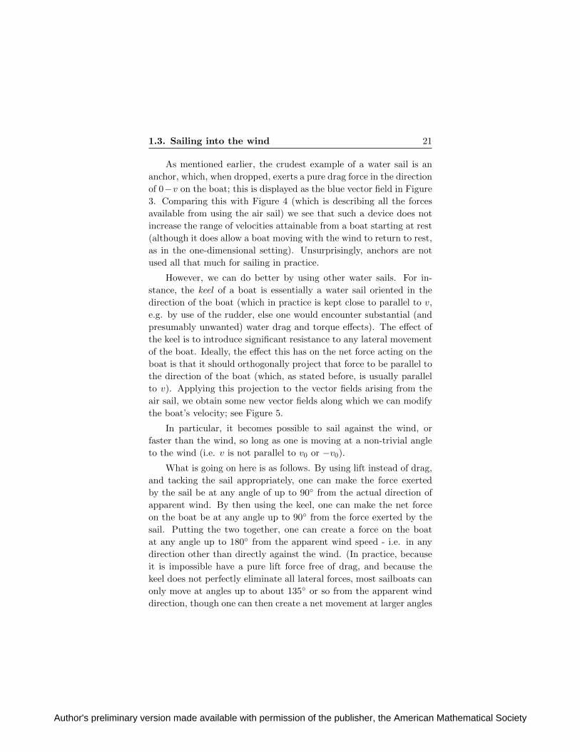
As mentioned earlier, the crudest example of a water sail is an

anchor, which, when dropped, exerts a pure drag force in the direction

of 0−v on the boat; this is displayed as the blue vector field in Figure

3. Comparing this with Figure 4 (which is describing all the forces

available from using the air sail) we see that such a device does not

increase the range of velocities attainable from a boat starting at rest

(although it does allow a boat moving with the wind to return to rest,

as in the one-dimensional setting). Unsurprisingly, anchors are not

used all that much for sailing in practice.

However, we can do better by using other water sails. For in-

stance, the keel of a boat is essentially a water sail oriented in the

direction of the boat (which in practice is kept close to parallel to v,

e.g. by use of the rudder, else one would encounter substantial (and

presumably unwanted) water drag and torque effects). The effect of

the keel is to introduce significant resistance to any lateral movement

of the boat. Ideally, the effect this has on the net force acting on the

boat is that it should orthogonally project that force to be parallel to

the direction of the boat (which, as stated before, is usually parallel

to v). Applying this projection to the vector fields arising from the

air sail, we obtain some new vector fields along which we can modify

the boat’s velocity; see Figure 5.

In particular, it becomes possible to sail against the wind, or

faster than the wind, so long as one is moving at a non-trivial angle

to the wind (i.e. v is not parallel to v0 or −v0).

What is going on here is as follows. By using lift instead of drag,

and tacking the sail appropriately, one can make the force exerted

by the sail be at any angle of up to 90 from the actual direction of

apparent wind. By then using the keel, one can make the net force

on the boat be at any angle up to 90 from the force exerted by the

sail. Putting the two together, one can create a force on the boat

at any angle up to 180 from the apparent wind speed - i.e. in any

direction other than directly against the wind. (In practice, because

it is impossible have a pure lift force free of drag, and because the

keel does not perfectly eliminate all lateral forces, most sailboats can

only move at angles up to about 135 or so from the apparent wind

direction, though one can then create a net movement at larger angles



Figure 5. The effect of a pure-drag sail (black), a pure-lift

sail (red), and a pure-lift sail combined with a keel (green).

Note that one now has the ability to shift the velocity v awayfrom both 0 and v0 no matter how fast one is already traveling,

so long as v is not collinear with 0 and v0.

by tacking and beating. For similar reasons, water drag prevents one

from using these methods to move too much faster than the wind

speed.)

In theory, one can also sail at any desired speed and direction by

combining the use of an air sail (or aerofoil) with the use of a water sail

(or hydrofoil). While water is a rather different fluid from air in many

respects (it is far denser, and virtually incompressible), one could in

principle deploy hydrofoils to exert lift forces on a boat perpendicular

to the apparent water velocity 0− v, much as an aerofoil can be used

to exert lift forces on the boat perpendicular to the apparent wind



velocity v0 − v. We saw in the previous section that if the effects of

air resistance somehow be ignored, then one could use lift to alter the

velocity v along a circle centred at the true wind speed v0; similarly, if

the effects of water resistance could also be ignored (e.g. by planing,

which reduces, but does not completely eliminate, these effects), then

one could alter the velocity v along a circle centred at the true water

speed 0. By alternately using the aerofoil and hydrofoil, one could in

principle reach arbitrarily large speeds and directions, as illustrated

in Figure 6.

I do not know however if one could actually implement such a

strategy with a physical sailing vessel. (Iceboats, however, have been

known to reach speeds of up to six times the wind speed or more,

though not exactly by the technique indicated in Figure 6. Thanks

to kanyonman for this fact.)

It is reasonable (in light of results such as the Kutta-Joukowski

theorem) to assume that the amount of lift provided by an aerofoil

or hydrofoil is linearly proportional to the apparent wind speed or

water speed. If so, then some basic trigonometry then reveals that

(assuming negligible drag) one can use either of the above techniques

to increase one’s speed at what is essentially a constant rate; in par-

ticular, one can reach speeds of n|v0| for any n > 0 in time O(n). On

the other hand, as drag forces are quadratically proportional to ap-

parent wind or water speed, one can decrease one’s speed at an very

rapid rate simply by dropping anchor; in fact one can drop speed from

n|v0| to |v0| in bounded time O(1) no matter how large n is! (This

fact is the time-reversal of the well-known fact that the Riccati ODE

u′ = u2 blows up in finite time.) These appear to be the best possible

rates for acceleration or deceleration using only air and water sails,

though I do not have a formal proof of this fact.


Izabella Laba pointed out several real-world sailing features not

covered by the above simplified model, notably the interaction be-

tween multiple sails, and noted that the model was closer in many

ways to windsurfing (or ice-sailing) than to traditional sailing.

Meichenl pointed out the relevance of the drag equation.



Figure 6. By alternating between a pure-lift aerofoil (red)

and a pure-lift hydrofoil (purple), one can in principle reach

arbitrarily large speeds in any direction.

1.4. The completeness and compactnesstheorems of first-order logic

The famous Godel completeness theorem in logic (not to be confused

with the even more famous Godel incompleteness theorem) roughly

states the following:


1.4. Completeness and compactness theorems 25

Theorem 1.4.1 (Godel completeness theorem, informal statement).

Let Γ be a theory (a formal language L, together with a set of ax-

ioms, i.e. sentences assumed to be true), and let φ be a sentence in

the formal language. Assume also that the language L has at most

countably many symbols. Then the following are equivalent:

(i) (Syntactic consequence) φ can be deduced from the axioms in

Γ by a finite number of applications of the laws of deduction

in first order logic. (This property is abbreviated as Γ ` φ.)

(ii) (Semantic consequence) Every structure U which satisfies

or models Γ, also satisfies φ. (This property is abbreviated

as Γ |= φ.)

(iii) (Semantic consequence for at most countable models) Every

structure U which is at most countable, and which models Γ,

also satisfies φ.

One can also formulate versions of the completeness theorem for

languages with uncountably many symbols, but I will not do so here.

One can also force other cardinalities on the model U by using the

Lowenheim-Skolem theorem.

To state this theorem even more informally, any (first-order) re-

sult which is true in all models of a theory, must be logically deducible

from that theory, and vice versa. (For instance, any result which is

true for all groups, must be deducible from the group axioms; any

result which is true for all systems obeying Peano arithmetic, must

be deducible from the Peano axioms; and so forth.) In fact, it suffices

to check countable and finite models only; for instance, any first-order

statement which is true for all finite or countable groups, is in fact true

for all groups! Informally, a first-order language with only countably

many symbols cannot “detect” whether a given structure is countably

or uncountably infinite. Thus for instance even the Zermelo-Frankel-

Choice (ZFC) axioms of set theory must have some at most countable

model, even though one can use ZFC to prove the existence of un-

countable sets; this is known as Skolem’s paradox. (To resolve the

paradox, one needs to carefully distinguish between an object in a

set theory being “externally” countable in the structure that models

that theory, and being “internally” countable within that theory.)



Of course, a theory Γ may contain undecidable statements φ -

sentences which are neither provable nor disprovable in the theory.

By the completeness theorem, this is equivalent to saying that φ is

satisfied by some models of Γ but not by other models. Thus the

completeness theorem is compatible with the incompleteness theorem:

recursively enumerable theories such as Peano arithmetic are modeled

by the natural numbers N, but are also modeled by other structures

also, and there are sentences satisfied by N which are not satisfied by

other models of Peano arithmetic, and are thus undecidable within

that arithmetic.

An important corollary of the completeness theorem is the com-

pactness theorem:

Corollary 1.4.2 (Compactness theorem, informal statement). Let

Γ be a first-order theory whose language has at most countably many

symbols. Then the following are equivalent:

(i) Γ is consistent, i.e. it is not possible to logically deduce a

contradiction from the axioms in Γ.

(ii) Γ is satisfiable, i.e. there exists a structure U that models

Γ.

(iii) There exists a structure U which is at most countable, that

models Γ.

(iv) Every finite subset Γ′ of Γ is consistent.

(v) Every finite subset Γ′ of Γ is satisfiable.

(vi) Every finite subset Γ′ of Γ is satisfiable with an at most

countable model.

Indeed, the equivalence of (i)-(iii), or (iv)-(vi), follows directly

from the completeness theorem, while the equivalence of (i) and (iv)

follows from the fact that any logical deduction has finite length and

so can involve at most finitely many of the axioms in Γ. (Again, the

theorem can be generalised to uncountable languages, but the models

become uncountable also.)

There is a consequence of the compactness theorem which more

closely resembles the sequential concept of compactness. Given a

sequence U1,U2, . . . be a sequence of structures for L, and another



structure U for L, let us say that Un converges elementarily to U if

every sentence φ which is satisfied by U, is also satisfied by Un for

sufficiently large n. (Replacing φ by its negation ¬φ, we also see

that every sentence that is not satisfied by U, is not satisfied by Unfor sufficiently large n.) Note that the limit U is only unique up to

elementary equivalence. Clearly, if each of the Un models some theory

Γ, then the limit U will also; thus for instance the elementary limit

of a sequence of groups is still a group, the elementary limit of a

sequence of rings is still a ring, etc.

Corollary 1.4.3 (Sequential compactness theorem). Let L be a lan-

guage with at most countably many symbols, and let U1,U2, . . . be a

sequence of structures for L. Then there exists a subsequence Unjwhich converges elementarily to a limit U which is at most countable.

Proof. For each structure Un, let Th(Un) be the theory of that struc-

ture, i.e. the set of all sentences that are satisfied by that structure.

One can view that theory as a point in 0, 1S , where S is the set

of all sentences in the language L. Since L has at most countably

many symbols, S is at most countable, and so (by the sequential

Tychonoff theorem) 0, 1S is sequentially compact in the product

topology. (This can also be seen directly by the usual Arzela-Ascoli

diagonalisation argument.) Thus we can find a subsequence Th(Unj )

which converges in the product topology to a limit theory Γ ∈ 0, 1S ,

thus every sentence in Γ is satisfied by Unj for sufficiently large j (and

every sentence not in Γ is not satisfied by Unj for sufficiently large j).

In particular, any finite subset of Γ is satisfiable, hence consistent;

by the compactness theorem, Γ itself is therefore consistent, and has

an at most countable model U. Also, each of the theories Th(Unj ) is

clearly complete (given any sentence φ, either φ or ¬φ is in the the-

ory), and so Γ is complete as well. One concludes that Γ is the theory

of U, and hence U is the elementary limit of the Unj as claimed.

Remark 1.4.4. It is also possible to state the compactness theorem

using the topological notion of compactness, as follows: let X be the

space of all structures of a given language L, quotiented by elementary

equivalence. One can define a topology on X by taking the sets

U ∈ X : U |= φ as a sub-base, where φ ranges over all sentences.



Then the compactness theorem is equivalent to the assertion that X

is topologically compact.

One can use the sequential compactness theorem to build a num-

ber of interesting “non-standard” models to various theories. For

instance, consider the language L used by Peano arithmetic (which

contains the operations +,× and the successor operation S, the rela-

tion =, and the constant 0), and adjoint a new constant N to create

an expanded language L ∪ N. For each natural number n ∈ N, let

Nn be a structure for L∪N which consists of the natural numbers

N (with the usual interpretations of +, ×, etc.) and interprets the

symbol N as the natural number n. By the compactness theorem,

some subsequence of Nn must converge elementarily to a new struc-

ture ∗N of L ∪ N, which still models Peano arithmetic, but now

has the additional property that N > n for every (standard) natural

number n; thus we have managed to create a non-standard model of

Peano arithmetic which contains a non-standardly large number (one

which is larger than every standard natural number).

The sequential compactness theorem also lets us construct infini-

tary limits of various sequences of finitary objects; for instance, one

can construct infinite pseudo-finite fields as the elementary limits of

sequences of finite fields. It also apepars to be related to a number

of correspondence principles between finitary and infinitary objects,

such as the Furstenberg correspondence principle between sets of in-

tegers and dynamical systems, or the more recent correspondence

principles concerning graph limits.

In this article, I will review the proof of the completeness (and

hence compactness) theorem. The material here is quite standard (I

basically follow the usual proof of Henkin, and taking advantage of

Skolemisation), but I wish to popularise the notion of an elementary

limit, which is not particularly well-known4.

4The closely related concept of an ultraproduct is better known, and can be usedto prove most of the compactness theorem already, thanks to Los’s theorem, but Ido not know how to use ultraproducts to ensure that the limiting model is countable.However, one can think (intuitively, at least), of the limit model U in the above theoremas being the set of “constructible” elements of an ultraproduct of the Un.



In order to emphasise the main ideas in the proof, I will gloss

over some of the more technical details in the proofs, relying instead

on informal arguments and examples at various points.

1.4.1. Completeness and compactness in propositional logic.

The completeness and compactness theorems are results in first-order

logic. But to motivate some of the ideas in proving these theorems, let

us first consider the simpler case of propositional logic. The language

L of a propositional logic consists of the following:

• A finite or infinite collection A1, A2, A3, . . . of propositional

variables - atomic formulae which could be true or false,

depending on the interpretation;

• A collection of logical connectives, such as conjunction ∧,

disjunction ∨, negation ¬, or implication =⇒ . (The exact

choice of which logical connectives to include in the language

is to some extent a matter of taste.)

• Parentheses (in order to indicate the order of operations).

Of course, we assume that the symbols used for atomic formulae

are distinct from those used for logical connectives, or for parenthe-

ses; we will implicitly make similar assumptions of this type in later

sections without further comment.

Using this language, one can form sentences (or formulae) by

some standard formal rules which I will not write down here. Typical

examples of sentences in propositional logic are A1 =⇒ (A2 ∨ A3),

(A1 ∧ ¬A1) =⇒ A2, and (A1 ∧ A2) ∨ (A1 ∧ A3). Each sentence

is of finite length, and thus involves at most finitely many of the

propositional variables. Observe that if L is at most countable, then

there are at most countably many sentences.

The analogue of a structure in propositional logic is a truth as-

signment. A truth assignment U for a propositional language L con-

sists of a truth value AUn ∈ true, false assigned to each propositional

variable An. (Thus, for instance, if there are N propositional vari-

ables in the language, then there are 2N possible truth assignments.)

Once a truth assignment U has assigned a truth value AUn to each

propositional variable An, it can then assign a truth value φU to any



other sentence φ in the language L by using the usual truth tables

for conjunction, negation, etc.; we write U |= φ if U assigns a true

value to φ (and say that φ is satisfied by U), and U 6|= φ otherwise.

Thus, for instance, if AU1 = false and AU

2 = true, then U |= A1 ∨ A2

and U |= A1 =⇒ A2, but U 6|= A2 =⇒ A1. Some sentences, e.g.

A1∨¬A1, are true in every truth assignment; these are the (semantic)

tautologies. At the other extreme, the negation of a tautology will of

course be false in every truth assignment.

A theory Γ is a language L, together with a (finite or infinite)

collection of sentences (also called Γ) in that language. A truth as-

signment U satisfies (or models) the theory Γ, and we write U |= Γ,

if we have U |= φ for all φ ∈ Γ. Thus, for instance, if U is as in the

preceding example and Γ := A1, A1 =⇒ A2, then U |= Γ.

The analogue of the Godel completeness theorem is then

Theorem 1.4.5 (Completeness theorem for propositional logic). Let

Γ be a theory for a propositional language L, and let φ be a sentence

in L. Then the following are equivalent:

(i) (Syntactic consequence) φ can be deduced from the axioms

in Γ by a finite number of applications of the laws of propo-

sitional logic.

(ii) (Semantic consequence) Every truth assignment U which sat-

isfies (or models) Γ, also satisfies φ.

One can list a complete set of laws of propositional logic used in

(i), but we will not do so here.

To prove the completeness theorem, it suffices to show the fol-

lowing equivalent version.

Theorem 1.4.6 (Completeness theorem for propositional logic, again).

Let Γ be a theory for a propositional language L. Then the following

are equivalent:

(i) Γ is consistent, i.e. it is not possible to logically deduce a

contradiction from the axioms in Γ.

(ii) Γ is satisfiable, i.e. there exists a truth assignment U that

models Γ.



Indeed, Theorem 1.4.5 follows from Theorem 1.4.6 by applying

Theorem 1.4.6 to the theory Γ ∪ ¬φ and taking contrapositives.

It remains to prove Theorem 1.4.6. It is easy to deduce (i) from

(ii), because the laws of propositional logic are sound : given any truth

assignment, it is easy to verify that these laws can only produce true

conclusions given true hypotheses. The more interesting implication

is to obtain (ii) from (i) - given a consistent theory Γ, one needs to

produce a truth assignment that models that theory.

Let’s first consider the case when the propositional language Lis finite, so that there are only finitely many propositional variables

A1, . . . , AN . Then we can argue using the following “greedy algo-

rithm”.

• We begin with a consistent theory Γ.

• Observe that at least one of Γ ∪ A1 or Γ ∪ ¬A1 must

be consistent. For if both Γ ∪ A1 and Γ ∪ ¬A1 led to a

logical contradiction, then by the laws of logic one can show

that Γ must also lead to a logical contradiction.

• If Γ ∪ A1 is consistent, we set AU1 := true and Γ1 :=

Γ∪A1; otherwise, we set AU1 := false and Γ1 := Γ∪¬A1.

• Γ1 is consistent, so arguing as before we know that at least

one of Γ1 ∪ A2 or Γ1 ∪ ¬A2 must be consistent. If the

former is consistent, we set AU2 := true and Γ2 := Γ1∪A2;

otherwise set AU2 := false and Γ2 := Γ1 ∪ ¬A2.

• We continue in this fashion, eventually ending up with a

consistent theory ΓN containing Γ, and a complete truth

assignment U such that An ∈ ΓN whenever 1 ≤ n ≤ N is

such that AUn = true, and such that ¬An ∈ ΓN whenever

1 ≤ n ≤ N is such that AUn = false.

• From the laws of logic and an induction argument, one then

sees that if φ is any sentence with φU = true, then φ is a

logical consequence of ΓN , and hence (since ΓN is consistent)

¬φ is not a consequence of ΓN . Taking contrapositives, we

see that φU = false whenever ¬φ is a consequence of ΓN ;

replacing φ by ¬φ we conclude that U satisfies every sentence

in ΓN , and the claim follows.



Remark 1.4.7. The above argument shows in particular that any

finite theory either has a model or a proof of a contradictory statement

(such as A ∧ ¬A). Actually producing a model if it exists, though, is

essentially the infamous satisfiability problem, which is known to be

NP-complete, and thus (if P 6= NP ) would require super-polynomial

time to execute.

The case of an infinite language can be obtained by combining

the above argument with Zorn’s lemma (or transfinite induction and

the axiom of choice, if the set of propositional variables happens to

be well-ordered). Alternatively, one can proceed by establishing

Theorem 1.4.8 (Compactness theorem for propositional logic). Let

Γ be a theory for a propositional language L. Then the following are

equivalent:

(i) Γ is satisfiable.

(ii) Every finite subset Γ′ of Γ is satisfiable.

It is easy to see that Theorem 1.4.8 will allow us to use the finite

case of Theorem 1.4.6 to deduce the infinite case, so it remains to

prove Theorem 1.4.8. The implication of (ii) from (i) is trivial; the

interesting implication is the converse.

Observe that there is a one-to-one correspondence between truth

assignments U and elements of the product space 0, 1A, where

A is the set of propositional variables. For every sentence φ, let

Fφ ⊂ 0, 1A be the collection of all truth assignments that satisfy

φ; observe that this is a closed (and open) subset of 0, 1A in the

product topology (basically because φ only involves finitely many of

the propositional variables). If every finite subset Γ′ of Γ is satisfi-

able, then⋃φ∈Γ′ Fφ is non-empty; thus the family (Fφ)φ∈Γ of closed

sets enjoys the finite intersection property. On the other hand, from

Tychonoff’s theorem, 0, 1A is compact. We conclude that⋂φ∈Γ Fφ

is non-empty, and the claim follows.

Remark 1.4.9. While Tychonoff’s theorem in full generality is equiv-

alent to the axiom of choice, it is possible to prove the compactness

theorem using a weaker version of this axiom, namely the ultrafilter



lemma. In fact, the compactness theorem is logically equivalent to

this lemma.

1.4.2. Zeroth-order logic. Propositional logic is far too limited

a language to do much mathematics. Let’s make the language a

bit more expressive, by adding constants, operations, relations, and

(optionally) the equals sign; however, we refrain at this stage from

adding variables or quantifiers, making this a zeroth-order logic rather

than a first-order one.

A zeroth-order language L consists of the following objects:

• A (finite or infinite) collection A1, A2, A3, . . . of proposi-

tional variables;

• A collection R1, R2, R3, . . . of relations (or predicates), with

each Ri having an arity (or valence) a[Ri] (e.g. unary rela-

tion, binary relation, etc.);

• A collection c1, c2, c3, . . . of constants;

• A collection f1, f2, f3, . . . of operators (or functions), with

each operator fi having an arity a[fi] (e.g. unary operator,

binary operator, etc.);

• Logical connectives;

• Parentheses;

• Optionally, the equals sign =.

For instance, a zeroth-order language for arithmetic on the nat-

ural numbers might include the constants 0, 1, 2, . . ., the binary re-

lations <,≤, >,≥, the binary operations +,×, the unary successor

operation S, and the equals sign =. A zeroth-order language for

studying all groups generated by six elements might include six gen-

erators a1, . . . , a6 and the identity element e as constants, as well as

the binary operation · of group multiplication and the unary opera-

tion ()−1 of group inversion, together with the equals sign =. And so

forth.

Note that one could shorten the description of such languages by

viewing propositional variables as relations of arity zero, and similarly

viewing constants as operators of arity zero, but I find it conceptually

clearer to leave these two operations separate, at least initially. As



we shall see shortly, one can also essentially eliminate the privileged

role of the equals sign = by treating it as just another binary relation,

which happens to have some standard axioms5 attached to it.

By combining constants and operators together in the usual fash-

ion one can create terms; for instance, in the zeroth-order language

for arithmetic, 3+(4×5) is a term. By inserting terms into a predicate

or relation (or the equals sign =), or using a propositional variable,

one obtains an atomic formula; thus for instance 3 + (4 × 5) > 25

is an atomic formula. By combining atomic formulae using logical

connectives, one obtains a sentence (or formula); thus for instance

((4× 5) > 22) =⇒ (3 + (4× 5) > 25) is a sentence.

In order to assign meaning to sentences, we need the notion of a

structure U for a zeroth-order language L. A structure consists of the

following objects:

• A domain of discourse (or universe of discourse) Dom(U);

• An assignment of a value cUn ∈ Dom(U) to every constant

cn;

• An assignment of a function fUn : Dom(U)a[fn] → Dom(U)

to every operation fn;

• An assignment of a truth value AUn ∈ true, false to every

propositional variable An;

• An assignment of a function RUn : Dom(U)a[Rn]true, false

to every relation Rn.

For instance, if L is the language of groups with six generators dis-

cussed above, then a structure U would consist of a set G = Dom(U),

seven elements aU1 , . . . , aU6 , e

U ∈ G in that set, a binary operation

·U : G × G → G, and a unary operation (()−1)U : G → G. At

present, no group-type properties are assumed on these operations;

the structure here is little more than a magma at this point.

Every sentence φ in a zeroth-order language L can be inter-

preted in a structure U for that language to give a truth value φU ∈true, false, simply by substituting all symbols α in the language

5Namely, that equality is reflexive, transitive, and symmetric, and can be substi-tuted in any expression to create an equal expression, or in any formula to create anequivalent formula.



with their interpreted counterparts αU (note that the equals sign =

does not need any additional data in order to be interpreted). For

instance, the sentence a1 · a2 = a3 is true in U if aU1 ·U aU2 = aU3 . Simi-

larly, every term t in the language can be interpreted to give a value

tU in the domain of discourse Dom(U).

As before, a theory is a collection of sentences; we can define

satisfiability U |= φ, U |= Γ of a sentence φ or a theory Γ by a structure

U just as in the previous section. For instance, to describe groups with

at most six generators in the language L, one might use the theory

Γ which consists of all the group axioms, specialised to terms, e.g.

Γ would contain the associativity axioms t1 · (t2 · t3) = (t1 · t2) · t3for all choices of terms t1, t2, t3. (Note that this theory is not quite

strong enough to capture the concept of a structure U being a group

generated by six elements, because the domain of U may contain some

“inaccessible” elements which are not the interpretation of any term

in L, but without the universal quantifier, there is not much we can

do in zeroth-order logic to say anything about those elements, and so

this is pretty much the best we can do with this limited logic.)

Now we can state the completeness theorem:

Theorem 1.4.10 (Completeness theorem for zeroth-order logic). Let

Γ be a theory for a zeroth-order language L, and let φ be a sentence

in L. Then the following are equivalent:

(i) (Syntactic consequence) φ can be deduced from the axioms

in Γ by a finite number of applications of the laws of zeroth-

order logic (i.e. all the laws of first-order logic that do not

involve variables or quantifiers).

(ii) (Semantic consequence) Every truth assignment U which sat-

isfies (or models) Γ, also satisfies φ.

To prove this theorem, it suffices as before to show that every con-

sistent theory Γ in a zeroth-order logic is satisfiable, and conversely.

The converse implication is again straightforward (the laws of zeroth-

order logic are easily seen to be sound); the main task is to show the

forward direction, i.e.

Proposition 1.4.11. Let Γ be a consistent zeroth-order theory. Then

Γ has at least one model.



Proof. It is convenient to begin by eliminating the equality sym-

bol from the language. Suppose we have already proven Proposition

1.4.11 has already been shown for languages without the equality

symbol. Then we claim that the proposition also holds for languages

with the equality symbol. Indeed, given a consistent theory Γ in a

language L with equality, we can form a companion theory Γ′ in the

language L′ formed by removing the equality symbol from L and re-

placing it with a new binary relation =′, by taking all the sentences

in Γ and replacing = by =′, and then adding in all the axioms of

equality (with = replaced by =′) to Γ′. Thus, for instance, one would

add the transitivity axioms (x =′ y) ∧ (y =′ z) =⇒ (x =′ z) to Γ

for each triple of terms x, y, z, as well as substitution axioms such as

(x =′ y) =⇒ (B(x, z) =′ B(y, z)) for any terms x, y, z and binary

functions B. It is straightforward to verify that if Γ is consistent,

then Γ′ is also consistent, because any contradiction derived in Γ′ can

be translated to a contradiction derived in Γ simply by replacing =′

with = throughout and using the axioms of equality. By hypothesis,

we conclude that Γ′ has some model U′. By the axioms of equality,

the interpretation (=′)U′

of =′ in this model is then an equivalence

relation on the domain Dom(U′) of U′. One can also remove from the

domain of U′ any element which is not of the form tU′

for some term

t, as such “inaccessible” elements will not influence the satisfiability

of Γ′. We can then define a structure U for the original language L by

quotienting the domain of U′ by the equivalence relation =′, and also

quotienting all the interpretations of the relations and operations of

L; the axioms of equality ensure that this quotienting is possible, and

that the quotiented structure U satisfies L; we omit the details.

Henceforth we assume that L does not contain the equality sign.

We will then choose a “tautological” domain of discourse Dom(U),

by setting this domain to be nothing more than the collection of all

terms in the language L. For instance, in the language of groups

on six generators, the domain Dom(U) is basically the free magma

(with “inverse”) on six generators plus an “identity”, consisting of

terms such as (a1 · a2)−1 · a1, (e · a3) · ((a4)−1)−1, etc. With this

choice of domain, there is an obvious “tautological” interpretation of

constants (cU := c) and operations (e.g. BU(t1, t2) := B(t1, t2)U for



binary operations B and terms t1, t2), which leads to every term t

being interpreted as itself: tU = t.

It remains to figure out how to interpret the propositional vari-

ables A1, A2, . . . and relations R1, R2, . . .. Actually, one can replace

each relation with an equivalent collection of new propositional vari-

ables by substituting in all possible terms in the relation. For instance,

if one has a binary relation R(, ), one can replace this single relation

symbol in the language by a (possibly infinite) collection of proposi-

tional variables R(t1, t2), one for each pair of terms t1, t2, leading to

a new (and probably much larger) language L without any relation

symbols. It is not hard to see that if theory Γ is consistent in L, then

the theory Γ in L formed by interpreting all atomic formulae such as

R(t1, t2) as propositional variables is also consistent. If Γ has a model

U with the tautological domain of discourse, it is not hard to see that

this can be converted to a model U of Γ with the same domain by

defining the interpretation RU of relations R in the obvious manner.

So now we may assume that there are no relation symbols, so that

Γ now consists entirely of propositional sentences involving the propo-

sitional variables. But the claim now follows from the completeness

theorem in propositional logic.

Remark 1.4.12. The above proof can be viewed as a combination

of the completeness theorem in propositional logic and the familiar

procedure in algebra of constructing an algebraic object (e.g. a group)

that obeys various relations, by starting with the free version of that

object (e.g. a free group) and then quotienting out by the equivalence

relation generated by those relations.

Remark 1.4.13. Observe that if L is at most countable, then the

structures U constructed by the above procedure are at most count-

able (because the set of terms is at most countable, and quotienting

by an equivalence relation cannot increase the cardinality). Thus we

see (as in Theorem 1.4.1 or Corollary 1.4.2) that if a zeroth-order

theory in an at most countable language is satisfiable, then it is in

fact satisfiable with an at most countable model.



From the completeness theorem for zeroth-order logic and the

above remark we obtain the compactness theorem for zeroth-order

logic, which is formulated exactly as in Corollary 1.4.2.

1.4.3. First-order logic. We are now ready to study languages

which are expressive enough to do some serious mathematics, namely

the languages of first-order logic, which are formed from zeroth-order

logics by adding variables and quantifiers. (There are higher-order

logics as well, but unfortunately the completeness and compactness

theorems typically fail for these, and they will not be discussed here.)

A language L for a first-order logic consists of the following:

• A (finite or infinite) collection A1, A2, A3, . . . of proposi-

tional variables;

• A collection R1, R2, R3, . . . of relations, with each Ri having

an arity a[Ri];

• A collection c1, c2, c3, . . . of constants;

• A collection f1, f2, f3, . . . of operators, with each fi having

an arity a[fi];

• A collection x1, x2, x3, . . . of variables;

• Logical connectives;

• The quantifiers ∀,∃;• Parentheses;

• Optionally, the equals sign =.

For instance, the language for Peano arithmetic includes a con-

stant 0, a unary operator S, binary operators +,×, the equals sign

=, and a countably infinite number of variables x1, x2, . . ..

By combining constants, variables and operators together one cre-

ates terms; by inserting terms into predicates or relations, or using

propositional variables, one obtains atomic formulae. These atomic

formulae can contain a number of free variables. Using logical con-

nectives as well as quantifiers to bind any or all of these variables, one

obtains well-formed formulae; a formula with no free variables is a

sentence. Thus, for instance, ∀x2 : x1 +x2 = x2 +x1 is a well-formed

formula, and ∀x1∀x2 : x1 + x2 = x2 + x1 is a sentence.



A structure U for a first-order language L is exactly the same con-

cept as for a zeroth-order language: a domain of discourse, together

with an interpretation of all the constants, operators, propositional

variables, and relations in the language. Given a structure U, one can

interpret terms t with no free variables as elements tU of Dom(U),

and interpret sentences φ as truth values φU ∈ true, false, in the

standard fashion.

A theory is, once again, a collection of sentences in the first-order

language L; one can define what it means for a structure to satisfy a

sentence or a theory just as before.

Remark 1.4.14. In most fields of mathematics, one wishes to dis-

cuss several types of objects (e.g. numbers, sets, points, group el-

ements, etc.) at once. For this, one would prefer to use a typed

language, in which variables, constants, and functions take values

in one type of object, and relations and functions take only certain

types of objects as input. However, one can easily model a typed

theory using a typeless theory by the trick of adding some additional

unary predicates to capture type (e.g. N(x) to indicate the asser-

tion “x is a natural number”, S(x) to indicate the assertion “x is a

set”, etc.) and modifying the axioms of the theory being considered

accordingly. (For instance, in a language involving both natural num-

bers and other mathematical objects, one might impose a new closure

axiom ∀x∀y : N(x) ∧ N(y) =⇒ N(x + y), and axioms such as the

commutativity axiom ∀x∀y : x+y = y+x would need to be modified

to ∀x∀y : N(x)∧N(y) =⇒ x+y = y+x.) It is a tedious but routine

matter to show that the completeness and compactness theorems for

typeless first-order logic imply analogous results for typed first-order

logic; we omit the details.

To prove the completeness (and hence compactness) theorem, it

suffices as before to show that

Proposition 1.4.15. Let Γ be a consistent first-order theory, with

an at most countable language L. Then Γ has at least one model U ,

which is also at most countable.

We shall prove this result using a series of reductions. Firstly, we

can mimic the arguments in the zeroth-order case and reduce to the



case when L does not contain the equality symbol. (We no longer

need to restrict the domain of discourse to those elements which can

be interpreted by terms, because the universal quantifier ∀ is now

available for use when stating the axioms of equality.) Henceforth we

shall assume that the equality symbol is not present in the language.

Next, by using the laws of first-order logic to push all quantifiers

in the sentences in Γ to the beginning (e.g. replacing (∀x : P (x)) ∧(∀y : Q(y)) with ∀x∀y : P (x) ∧ Q(y)) one may assume that all sen-

tences in Γ are in prenex normal form, i.e. they consist of a “matrix”

of quantifiers, followed by an quantifier-free formula - a well-formed

formula with no quantifiers. For instance, ∀x∃y∀z∃w : P (x, y, z, w)

is in prenex normal form, where P (x, y, z, w) is an quantifier-free for-

mula with four free variables x, y, z, w.

Now we will start removing the existential quantifiers ∃ from the

sentences in Γ. Let’s begin with a simple case, when Γ contains a

sentence of the form ∃x : P (x) for some quantifier-free formula of one

free variable x. Then one can eliminate the existential quantifier by

introducing a witness, or more precisely adjoining a new constant c

to the language L and replacing the statement ∃x : P (x) with the

statement P (c), giving rise to a new theory Γ′ in a new language

Λ′. The consistency of Γ easily implies the consistency of Γ′, while

any at most countable model for Γ′ can be easily converted to an at

most countable model for Γ (by “forgetting” the symbol c). (In fact,

Γ′ is a conservative extension of Γ.) We can apply this reduction

simultaneously to all sentences of the form ∃x : P (x) in Γ (thus

potentially expanding the collection of constants in the language by

a countable amount).

The same argument works for any sentence in prenex normal form

in which all the existential quantifiers are to the left of the universal

quantifiers, e.g. ∃x∃y∀z∀w : P (x, y, z, w); this statement requires two

constants to separately witness x and y, but otherwise one proceeds

much as in the previous paragraph. But what about if one or more

of the existential quantifiers is buried behind a universal quantifier?

The trick is then to use Skolemisation. We illustrate this with the

simplest case of this type, namely that of a sentence ∀x∃y : P (x, y).

Here, one cannot use a constant witness for y. But this is no problem:



one simply introduces a witness that depends on x. More precisely,

one adjoins a new unary operator c to the language L and replaces the

statement ∀x∃y : P (x, y) by ∀x : P (x, c(x)), creating a new theory

Γ′ in a new language Λ′. One can again show (though this is not

entirely trivial) that the consistency of Γ implies the consistency of

Γ′, and that every countable model for Γ′ can be converted to a

countable model for Γ (again by “forgetting” c). So one can eliminate

the existential quantifier from this sentence also. Similar methods

work for any other prenex normal form; for instance with the sentence

∀x∃y∀z∃w : P (x, y, z, w)

one can obtain a conservative extension of that theory by introducing

a unary operator c and a binary operator d and replacing the above

sentence with

∀x∀z : P (x, c(x), z, d(x, z)).

One can show that one can perform Skolemisation on all the sentences

in Γ simultaneously, which has the effect of eliminating all existential

quantifiers from Γ while still keeping the language L at most countable

(since Γ is at most countable). (Intuitively, what is going on here

is that we are interpreting all existential axioms in the theory as

implicitly defining functions, which we then explicitly formalise as a

new symbol in the language. For instance, if we had some theory of

sets which contained the axiom of choice (every family of non-empty

sets (Xα)α∈A admits a choice function f : A →⋃α∈AXα), then we

can Skolemise this by introducing a “choice function function” F :

(Xα)α∈A 7→ F((Xα)α∈A) that witnessed this axiom to the language.

Note that we do not need uniqueness in the existential claim in order

to be able to perform Skolemisation.)

After performing Skolemisation and adding all the witnesses to

the language, we are reduced to the case in which all the sentences

in Γ are in fact universal statements, i.e. of the form ∀x1 . . . ∀xk :

P (x1, . . . , xk), where P (x1, . . . , xk) is an quantifier-free formula of k

free variables. In this case one can repeat the zeroth-order arguments,

selecting a structure U whose domain of discourse is the tautological

one, indexed by all the terms with no free variables (in particular, this

structure will be countable). One can then replace each first-order



statement ∀x1 . . . ∀xk : P (x1, . . . , xk) in Γ by the family of zeroth-

order statements P (t1, . . . , tk), where t1, . . . , tk ranges over all terms

with no free variables, thus creating a zeroth-order theory Γ0. As Γ

is consistent, Γ0 is also, so by the zeroth-order theory, we can find a

model U for Γ0 with the tautological domain of discourse, and it is

clear that this structure will also be a model for the original theory

Γ. The proof of the completeness theorem (and thus the compactness

theorem) is now complete.

In summary: to create a countable model from a consistent first-

order theory, one first replaces the equality sign = (if any) by a binary

relation =′, then uses Skolemisation to make all implied functions and

operations explicit elements of the language. Next, one makes the

zeroth-order terms of the new language the domain of discourse, ap-

plies a greedy algorithm to decide the truth assignment of all zeroth-

order sentences, and then finally quotients out by the equivalence

relation given by =′ to recover the countable model.

Remark 1.4.16. I find the use of Skolemisation to greatly clarify,

at a conceptual level, the proof of the completeness theorem. How-

ever, at a technical level it does make things more complicated: in

particular, showing that the Skolemisation of a consistent theory is

still consistent does require some non-trivial effort (one has to take

all arguments involving the Skolem function c(), and replace every

occurence of c() by a “virtual” function, defined implicitly using ex-

istential quantifiers). On the other hand, this fact is easy to prove

once one already has the completeness theorem, though we of course

cannot formally take advantage of this while trying to prove that

theorem!

The more traditional Henkin approach is based instead on adding

a large number of constant witnesses, one for every existential state-

ment: roughly speaking, for each existential sentence ∃x : P (x) in the

language, one adds a new constant c to the language and inserts an

axiom (∃x : P (x)) =⇒ P (c) to the theory; it is easier to show that

this preserves consistency than it is with a more general Skolemisa-

tion. Unfortunately, every time one adds a constant to the language,

one increases the number of existential sentences for which one needs

to perform this type of witnessing, but it turns out that after applying


1.5. Talagrand’s concentration inequality 43

this procedure a countable number of times, one can get to the point

where every existential sentence is automatically witnessed by some

constant. This has the same ultimate effect as Skolemisation, namely

one can convert sentences containing existential quantifiers to ones

which are purely universal, and so the rest of the proof is much the

same as the proof described above. On the other hand, the Henkin

approach avoids the axiom of choice (though one still must use the

ultrafilter lemma, of course).


Thanks to Carson Chow, Ernie Cohen, Eric, John Goodrick, and

anonymous commenters for corrections.

1.5. Talagrand’s concentration inequality

In the theory of discrete random matrices (e.g. matrices whose entries

are random signs ±1), one often encounters the problem of under-

standing the distribution of the random variable dist(X,V ), where

X = (x1, . . . , xn) ∈ −1,+1n is an n-dimensional random sign vec-

tor (so X is uniformly distributed in the discrete cube −1,+1n),

and V is some d-dimensional subspace of Rn for some 0 ≤ d ≤ n.

It is not hard to compute the second moment of this random vari-

able. Indeed, if P = (pij)1≤i,j≤n denotes the orthogonal projection

matrix from Rn to the orthogonal complement V ⊥ of V , then one

observes that

dist(X,V )2 = X · PX =n∑i=1

n∑j=1

xixjpij

and so upon taking expectations we see that

(1.23) E dist(X,V )2 =n∑i=1

pii = trP = n− d

since P is a rank n−d orthogonal projection. So we expect dist(X,V )

to be about√n− d on the average.

In fact, one has sharp concentration around this value, in the

sense that dist(X,V ) =√n− d + O(1) with high probability. More

precisely, we have



Proposition 1.5.1 (Large deviation inequality). For any t > 0, one

has

P(|dist(X,V )−√n− d| ≥ t) ≤ C exp(−ct2)

for some absolute constants C, c > 0.

In fact the constants C, c are very civilised; for large t one can

basically take C = 4 and c = 1/16, for instance. This type of con-

centration, particularly for subspaces V of moderately large codimen-

sion6 n− d, is fundamental to much of my work on random matrices

with Van Vu, starting with our first paper[TaVu2006] (in which this

proposition first appears).

Proposition 1.5.1 is an easy consequence of the second moment

computation and Talagrand’s inequality [Ta1996], which among other

things provides a sharp concentration result for convex Lipschitz func-

tions on the cube −1,+1n; since dist(x, V ) is indeed a convex Lips-

chitz function, this inequality can be applied immediately. The proof

of Talagrand’s inequality is short and can be found in several text-

books (e.g. [AlSp2008]), but I thought I would reproduce the argu-

ment here (specialised to the convex case), mostly to force myself to

learn the proof properly. Note the concentration of O(1) obtained by

Talagrand’s inequality is much stronger than what one would get from

more elementary tools such as Azuma’s inequality or McDiarmid’s in-

equality, which would only give concentration of about O(√n) or so

(which is in fact trivial, since the cube −1,+1n has diameter 2√n);

the point is that Talagrand’s inequality is very effective at exploiting

the convexity of the problem, as well as the Lipschitz nature of the

function in all directions, whereas Azuma’s inequality can only easily

take advantage of the Lipschitz nature of the function in coordinate

directions. On the other hand, Azuma’s inequality works just as well

if the `2 metric is replaced with the larger `1 metric, and one can con-

clude that the `1 distance between X and V concentrates around its

median to a width O(√n), which is a more non-trivial fact than the

`2 concentration bound given by that inequality. (The computation

6For subspaces of small codimension (such as hyperplanes) one has to use othertools to get good results, such as inverse Littlewood-Offord theory or the Berry-Esseencentral limit theorem, but that is another story.



of the median of the `1 distance is more complicated than for the `2

distance, though, and depends on the orientation of V .)

Remark 1.5.2. If one makes the coordinates of X iid Gaussian vari-

ables xi ≡ N(0, 1) rather than random signs, then Proposition 1.5.1 is

much easier to prove; the probability distribution of a Gaussian vec-

tor is rotation-invariant, so one can rotate V to be, say, Rd, at which

point dist(X,V )2 is clearly the sum of n − d independent squares of

Gaussians (i.e. a chi-square distribution), and the claim follows from

direct computation (or one can use the Chernoff inequality). The

gaussian counterpart of Talagrand’s inequality is more classical, be-

ing essentially due to Levy, and will also be discussed later in this

post.

1.5.1. Concentration on the cube. Proposition 1.5.1 follows eas-

ily from the following statement, that asserts that if a convex set

A ⊂ Rn occupies a non-trivial fraction of the cube −1,+1n, then

the neighbourhood At := x ∈ Rn : dist(x,A) ≤ t will occupy

almost all of the cube for t 1:

Proposition 1.5.3 (Talagrand’s concentration inequality). Let A be

a convex set in Rd. Then

P(X ∈ A)P(X 6∈ At) ≤ exp(−ct2)

for all t > 0 and some absolute constant c > 0, where X ∈ −1,+1nis chosen uniformly from −1,+1n.

Remark 1.5.4. It is crucial that A is convex here. If instead A

is, say, the set of all points in −1,+1n with fewer than n/2 −√n

+1’s, then P(X ∈ A) is comparable to 1, but P(X 6∈ At) only starts

decaying once t √n, rather than t 1. Indeed, it is not hard to

show that Proposition 1.5.3 implies the variant

P(X ∈ A)P(X 6∈ At) ≤ exp(−ct2/n)

for non-convex A (by restricting A to −1,+1n and then passing

from A to the convex hull, noting that distances to A on −1,+1nmay be contracted by a factor of O(

√n) by this latter process); this

inequality can also be easily deduced from Azuma’s inequality.



To apply this proposition to the situation at hand, observe that

if A is the cylindrical region x ∈ Rn : dist(x, V ) ≤ r for some r,

then A is convex and At is contained in x ∈ Rn : dist(x, V ) ≤ r+ t.Thus

P(dist(X,V ) ≤ r)P(dist(X,V ) > r + t) ≤ exp(−ct2).

Applying this with r := M or r := M−t, where M is the median value

of dist(X,V ), one soon obtains concentration around the median:

P(|dist(X,V )−M | > t) ≤ 4 exp(−ct2).

This is only compatible with (1.23) if M =√n− d + O(1), and the

claim follows.

To prove Proposition 1.5.3, we use the exponential moment method.

Indeed, it suffices by Markov’s inequality to show that

(1.24) P(X ∈ A)E exp(cdist(X,A)2) ≤ 1

for a sufficiently small absolute constant c > 0 (in fact one can take

c = 1/16).

We prove (1.24) by an induction on the dimension n. The claim

is trivial for n = 0, so suppose n ≥ 1 and the claim has already been

proven for n− 1.

Let us write X = (X ′, xn) for xn = ±1. For each t ∈ R, we

introduce the slice At := x′ ∈ Rn−1 : (x′, t) ∈ A, then At is convex.

We now try to bound the left-hand side of (1.24) in terms of X ′, Atrather than X,A. Clearly

P(X ∈ A) =1

2[P(X ′ ∈ A−1) + P(X ′ ∈ A+1)].

By symmetry we may assume that P(X ′ ∈ A+1) ≥ P(X ′ ∈ A−1),

thus we may write

(1.25) P(X ′ ∈ A±1) = p(1± q)

where p := P(X ∈ A) and 0 ≤ q ≤ 1.

Now we look at dist(X,A)2. For t = ±1, let Yt ∈ Rn−1 be the

closest point of (the closure of) At to X ′, thus

(1.26) |X ′ − Yt| = dist(X ′, At).



Let 0 ≤ λ ≤ 1 be chosen later; then the point (1 − λ)(Yxn , xn) +

λ(Y−xn ,−xn) lies in A by convexity, and so

dist(X,A) ≤ |(1− λ)(Yxn , xn) + λ(Y−xn ,−xn)− (X ′, xn)|.

Squaring this and using Pythagoras, one obtains

dist(X,A)2 ≤ 4λ2 + |(1− λ)(X ′ − Yxn) + λ(X ′ − Y−xn)|2.

As we will shortly be exponentiating the left-hand side, we need to lin-

earise the right-hand side. Accordingly, we will exploit the convexity

of the function x 7→ |x|2 to bound

|(1− λ)(X − Yxn) + λ(X − Y−xn)|2 ≤

(1− λ)|X ′ − Yxn |2 + λ|X ′ − Y−xn |2

and thus by (1.26)

dist(X,A)2 ≤ 4λ2 + (1− λ) dist(X ′, Axn)2 + λdist(X ′, A−xn)2.

We exponentiate this and take expectations in X ′ (holding xn fixed

for now) to get

EX′ec dist(X,A)2 ≤ e4cλ2

EX′(ec dist(X′,Axn )2)1−λ(ec dist(X′,A−xn )2)λ.

Meanwhile, from the induction hypothesis and (1.25) we have

EX′ec dist(X′,Axn )2 ≤ 1

p(1 + xnq)

and similarly for A−xn . By Holder’s inequality, we conclude

EX′ec dist(X,A)2 ≤ e4cλ2 1

p(1 + xnq)1−λ(1− xnq)λ.

For xn = +1, the optimal choice of λ here is 0, obtaining

EX′ec dist(X,A)2 =

1

p(1 + q);

for xn = −1, the optimal choice of λ is to be determined. Averaging,

we obtain

EXec dist(X,A)2 =

1

2[

1

p(1 + q)+ e4cλ2 1

p(1− q)1−λ(1 + q)λ]

so to establish (1.24), it suffices to pick 0 ≤ λ ≤ 1 such that

1

1 + q+ e4cλ2 1

(1− q)1−λ(1 + q)λ≤ 2.



If q is bounded away from zero, then by choosing λ = 1 we would

obtain the claim if c is small enough, so we may take q to be small.

But then a Taylor expansion allows us to conclude if we take λ to be

a constant multiple of q, and again pick c to be small enough. The

point is that λ = 0 already almost works up to errors of O(q2), and

increasing λ from zero to a small non-zero quantity will decrease the

LHS by about O(λq)−O(cλ2).

By optimising everything using first-year calculus, one eventually

gets the constant c = 1/16 claimed earlier.

Remark 1.5.5. Talagrand’s inequality is in fact far more general

than this; it applies to arbitrary products of probability spaces, rather

than just to −1,+1n, and to non-convex A, but the notion of dis-

tance needed to define At becomes more complicated; the proof of

the inequality, though, is essentially the same. Besides its applicabil-

ity to convex Lipschitz functions, Talagrand’s inequality is also very

useful for controlling combinatorial Lipschitz functions F which are

“locally certifiable” in the sense that whenever F (x) is larger than

some threshold t, then there exist some bounded number f(t) of co-

efficients of x which “certify” this fact (in the sense that F (y) ≥ t

for any other y which agrees with x on these coefficients). See e.g.

[AlSp2008] for a more precise statement and some applications.

1.5.2. Gaussian concentration. As mentioned earlier, there are

analogous results when the uniform distribution on the cube −1,+1nare replaced by other distributions, such as the n-dimensional Gauss-

ian distribution. In fact, in this case convexity is not needed:

Proposition 1.5.6 (Gaussian concentration inequality). Let A be a

measurable set in Rd. Then

P(X ∈ A)P(X 6∈ At) ≤ exp(−ct2)

for all t > 0 and some absolute constant c > 0, where X ≡ N(0, 1)n

is a random Gaussian vector.

This inequality can be deduced from Levy’s classical concentra-

tion of measure inequality for the sphere (with the optimal constant),

but we will give an alternate proof due to Maurey and Pisier. It

suffices to prove the following variant of Proposition 1.5.6:



Proposition 1.5.7 (Gaussian concentration inequality for Lipschitz

functions). Let f : Rd → R be a function which is Lipschitz with

constant 1 (i.e. |f(x) − f(y)| ≤ |x − y| for all x, y ∈ Rd). Then for

any t we have

P(|f(X)−Ef(X)| ≥ t) ≤ exp(−ct2)

for all t > 0 and some absolute constant c > 0, where X ≡ N(0, 1)n

is a random variable.

Indeed, if one sets f(x) := dist(x,A) one can soon deduce Propo-

sition 1.5.6 from Proposition 1.5.7.

Informally, Proposition 1.5.7 asserts that Lipschitz functions of

Gaussian variables concentrate as if they were Gaussian themselves;

for comparison, Talagrand’s inequality implies that convex Lipschitz

functions of Bernoulli variables concentrate as if they were Gaussian.

Now we prove Proposition 1.5.7. By the epsilon regularisation

argument (Section 2.7 of Volume I ) we may take f to be smooth,

and so by the Lipschitz property we have

(1.27) |∇f(x)| ≤ 1

for all x. By subtracting off the mean we may assume Ef = 0. By

replacing f with −f if necessary it suffices to control the upper tail

probability P(f(X) ≥ t) for t > 0.

We again use the exponential moment method. It suffices to show

that

E exp(tf(X)) ≤ exp(Ct2)

for some absolute constant C.

Now we use a variant of the square and rearrange trick. Let Y be

an independent copy of X. Since Ef(Y ) = 0, we see from Jensen’s

inequality that E exp(−tf(Y )) ≥ 1, and so

E exp(tf(X)) ≤ E exp(t(f(X)− f(Y ))).

With an eye to exploiting (1.27), one might seek to use the funda-

mental theorem of calculus to write

f(X)− f(Y ) =

∫ 1

0

d

dλf((1− λ)Y + λX) dλ.



But actually it turns out to be smarter to use a circular arc of inte-

gration, rather than a line segment:

f(X)− f(Y ) =

∫ π/2

0

d

dθf(Y cos θ +X sin θ) dθ.

The reason for this is that Xθ := Y cos θ + X sin θ is another gauss-

ian random variable equivalent to N(0, 1)n, as is its derivative X ′θ :=

−Y sin θ+X cos θ; furthermore, and crucially, these two random vari-

ables are independent.

To exploit this, we first use Jensen’s inequality to bound

exp(t(f(X)− f(Y ))) ≤ π

2

∫ π/2

0

exp(2t

π

d

dθf(Xθ)) dθ.

Applying the chain rule and taking expectations, we have

E exp(t(f(X)− f(Y ))) ≤ π

2

∫ π/2

0

E exp(2t

π∇f(Xθ) ·X ′θ) dθ.

Let us condition Xθ to be fixed, then X ′θ ≡ N(0, 1)n; applying (1.27),

we conclude that 2tπ∇f(Xθ)·X ′θ is normally distributed with standard

deviation at most 2tπ . As such we have

E exp(2t

π∇f(Xθ) ·X ′θ) ≤ exp(Ct)

for some absolute constant C; integrating out the conditioning on Xθ

we obtain the claim.


Thanks to Oded and vedadi for corrections.

1.6. The Szemeredi-Trotter theorem and the celldecomposition

The celebrated Szemeredi-Trotter theorem gives a bound for the set

of incidences I(P,L) := (p, `) ∈ P × L : p ∈ ` between a finite

set of points P and a finite set of lines L in the Euclidean plane R2.

Specifically, the bound is

(1.28) |I(P,L)| |P |2/3|L|2/3 + |P |+ |L|

where we use the asymptotic notation X Y or X = O(Y ) to

denote the statement that X ≤ CY for some absolute constant C.


1.6. The cell decomposition 51

In particular, the number of incidences between n points and n lines

is O(n4/3). This bound is sharp; consider for instance the discrete

box P := (a, b) ∈ Z2 : 1 ≤ a ≤ N ; 1 ≤ b ≤ 2N2 with L being the

collection of lines (x,mx + b) : m, b ∈ Z, 1 ≤ m ≤ N, 1 ≤ b ≤ N2.One easily verifies that |P | = 2N3, |L| = N3, and |I(P,L)| = N4,

showing that (1.28) is essentially sharp in the case |P | ∼ |L|; one can

concoct similar examples for other regimes of |P | and |L|.On the other hand, if one replaces the Euclidean plane R2 by a

finite field geometry F 2, where F is a finite field, then the estimate

(1.28) is false. For instance, if P is the entire plane F 2, and L is

the set of all lines in F 2, then |P |, |L| are both comparable to |F |2,

but |I(P,L)| is comparable to |F |3, thus violating (1.28) when |F | is

large. Thus any proof of the Szemeredi-Trotter theorem must use a

special property of the Euclidean plane which is not enjoyed by finite

field geometries. In particular, this strongly suggests that one cannot

rely purely on algebra and combinatorics to prove (1.28); one must

also use some Euclidean geometry or topology as well.

Nowadays, the slickest proof of the Szemeredi-Trotter theorem is

via the crossing number inequality (as discussed in Section 1.10 of

Structure and Randomness), which ultimately relies on Euler’s for-

mula |V |− |E|+ |F | = 2; thus in this argument it is topology which is

the feature of Euclidean space which one is exploiting, and which is

not present in the finite field setting. In this article, though, I would

like to mention a different proof (closer in spirit to the original proof

of Szemeredi-Trotter [SzTr1983], and closer still to the later paper

[ClEdGuShWe1990]), based on the method of cell decomposition,

which has proven to be a very flexible method in combinatorial inci-

dence geometry. Here, the distinctive feature of Euclidean geometry

one is exploiting is convexity, which again has no finite field analogue.

Roughly speaking, the idea is this. Using nothing more than the

axiom that two points determine at most one line, one can obtain the

bound

(1.29) |I(P,L)| |P ||L|1/2 + |L|,

which is inferior to (1.28). (On the other hand, this estimate works in

both Euclidean and finite field geometries, and is sharp in the latter



case, as shown by the example given earlier.) Dually, the axiom that

two lines determine at most one point gives the bound

(1.30) |I(P,L)| |L||P |1/2 + |P |

(or alternatively, one can use projective duality to interchange points

and lines and deduce (1.30) from (1.29)).

An inspection of the proof of (1.29) shows that it is only expected

to be sharp when the bushes Lp := ` ∈ L : ` 3 p associated to each

point p ∈ P behave like “independent” subsets of L, so that there is

no significant correlation between the bush Lp of one point and the

bush of another point Lq.

However, in Euclidean space, we have the phenomenon that the

bush of a point Lp is influenced by the region of space that p lies in.

Clearly, if p lies in a set Ω (e.g. a convex polygon), then the only lines

` ∈ L that can contribute to Lp are those lines which pass through

Ω. If Ω is a small convex region of space, one expects only a fraction

of the lines in L to actually pass through Ω. As such, if p and q

both lie in Ω, then Lp and Lq are compressed inside a smaller subset

of L, namely the set of lines passing through Ω, and so should be

more likely to intersect than if they were independent. This should

lead to an improvement to (1.29) (and indeed, as we shall see below,

ultimately leads to (1.28)).

More formally, the argument proceeds by applying the following

lemma:

Lemma 1.6.1 (Cell decomposition). Let L be a finite collection of

lines in R2, and let r ≥ 1. Then it is possible to find a set R of O(r)

lines in the plane (which may or may not be in L), which subdivide

R2 into O(r2) convex regions (or cells), such that the interior of each

such cell is incident to at most O(|L|/r) lines.

The deduction of (1.28) from (1.29), (1.30) and Lemma 1.6.1 is

very quick. Firstly we may assume we are in the range

(1.31) |L|1/2 |P | |L|2

otherwise the bound (1.28) follows already from either (1.29) or (1.30)

and some high-school algebra.



Let r ≥ 1 be a parameter to be optimised later. We apply the

cell decomposition to subdivide R2 into O(r2) open convex regions,

plus a family R of O(r) lines. Each of the O(r2) convex regions

Ω has only O(|L|/r) lines through it, and so by (1.29) contributes

O(|P ∩ Ω||L|1/2/r1/2 + |L|/r) incidences. Meanwhile, on each of the

lines ` in R used to perform this decomposition, there are at most

|L| transverse incidences (because each line in L distinct from ` can

intersect ` at most once), plus all the incidences along ` itself. Putting

all this together, one obtains

|I(P,L)| ≤ |I(P,L ∩R)|+O(|P ||L|1/2/r1/2 + |L|r).

We optimise this by selecting r ∼ |P |2/3/|L|1/3; from (1.31) we can

ensure that r ≤ |L|/2, so that |L ∩R| ≤ |L|/2. One then obtains

|I(P,L)| ≤ |I(P,L ∩R)|+O(|P |2/3|L|2/3).

We can iterate away the L∩R error (halving the number of lines each

time) and sum the resulting geometric series to obtain (1.28).

It remains to prove (1.6.1). If one subdivides R2 using r arbitrary

lines, one creates at most O(r2) cells (because each new line intersects

the existing lines at most once, and so can create at most O(r) distinct

cells), and for a similar reason, every line in L visits at most r of

these regions, and so by double counting one expects O(|L|/r) lines

per cell “on the average”. The key difficulty is then to get O(|L|/r)lines through every cell, not just on the average. It turns out that a

probabilistic argument will almost work, but with a logarithmic loss

(thus having O(|L| log |L|/r) lines per cell rather than O(|L|/r)); but

with a little more work one can then iterate away this loss also. The

arguments here are loosely based on those of [ClEdGuShWe1990];

a related (deterministic) decomposition also appears in [SzTr1983].

But I wish to focus here on the probabilistic approach.

It is also worth noting that the original (somewhat complicated)

argument of Szemeredi-Trotter has been adapted to establish the ana-

logue of (1.28) in the complex plane C2 by Toth[To2005], while the

other known proofs of Szemeredi-Trotter, so far, have not been able to

be extended to this setting (the Euler characteristic argument clearly

breaks down, as does any proof based on using lines to divide planes



into half-spaces). So all three proofs have their advantages and dis-

advantages.

1.6.1. The trivial incidence estimate. We first give a quick proof

of the trivial incidence bound (1.29). We have

|I(P,L)| =∑`∈L

|P ∩ `|

and thus by Cauchy-Schwarz∑`∈L

|P ∩ `|2 ≥ |I(P,L)|2

|L|.

On the other hand, observe that∑`∈L

|P ∩ `|2 − |P ∩ `| = |(p, q, `) ∈ P × P × L : p 6= q; p, q ∈ `.

Because two distinct points p, q are incident to at most one line, the

right-hand side is at most |P |2, thus∑`∈L

|P ∩ `|2 ≤ |I(P,L)|+ |P |2.

Comparing this with the Cauchy-Schwarz bound and using a little

high-school algebra we obtain (1.29). A dual argument (swapping

the role of lines and points) give (1.30).

A more informal proof of (1.29) can be given as follows. Suppose

for contradiction that |I(P,L)| was much larger than |P ||L|1/2 + |L|.Since |I(P,L)| =

∑p∈P |Lp|, this implies that that the |Lp| are much

larger than |L|1/2 on the average. By the birthday paradox, one then

expects two randomly chosen Lp, Lq to intersect in at least two places

`, `′; but this would mean that two lines intersect in two points, a con-

tradiction. The use of Cauchy-Schwarz in the rigorous argument given

above can thus be viewed as an assertion that the average intersection

of Lp and Lq is at least as large as what random chance predicts.

As mentioned in the introduction, we now see (intuitively, at

least) that if nearby p, q are such that Lp, Lq are drawn from a smaller

pool of lines than L, then their intersection is likely to be higher, and

so one should be able to improve upon (1.29).



1.6.2. The probabilistic bound. Now we start proving Lemma

1.6.1. We can assume that r < |L|, since the claim is trivial otherwise

(we just use all the lines in L to subdivide the plane, and there are

no lines left in L to intersect any of the cells). Similarly we may

assume that r > 1, and that |L| is large. We can also perturb all

the lines slightly and assume that the lines are in general position

(no three are concurrent), as the general claim then follows from

a limiting argument (note that this may send some of the cells to

become empty). (Of course, the Szemeredi-Trotter theorem is quite

easy under the assumption of general position, but this theorem is

not our current objective right now.)

We use the probabilistic method, i.e. we construct R by some

random recipe and aim to show that the conclusion of the lemma

holds with positive probaility.

The most obvious approach would be to choose the r lines R

at random from L, thus each line ` ∈ L has a probability of r/|L|of lying in R. Actually, for technical reasons it is slightly better

to use a Bernoulli process to select R, thus each line ` ∈ L lies in

R with an independent probability of r/|L|. This can cause R to

occasionally have size much larger than r, but this probability can be

easily controlled (e.g. using the Chernoff inequality). So with high

probability, R consists of O(r) lines, which therefore carve out O(r2)

cell. The remaining task is to show that each cell is incident to at

most O(|L|/r) lines from L.

Observe that each cell is a (possibly unbounded) polygon, whose

edges come from lines in R. Note that (except in the degenerate case

when R consists of at most one line, which we can ignore) any line `

which meets a cell in R, must intersect at least one of the edges of R.

If we pretend for the moment that all cells have a bounded number

of edges, it would then suffice to show that each edge of each cell was

incident to O(|L|/r) lines.

Let’s see how this would go. Suppose that one line ` ∈ L was

picked for the set R, and consider all the other lines in L that inter-

sect `; there are O(|L|) of these lines `′, which (by the general position

hypothesis) intersect ` at distinct points ` ∩ `′ on the line. If one of



these lines `′ intersecting ` is also selected for R, then the correspond-

ing point `∩ `′ will become a vertex of one of the cells (indeed, it will

be the vertex of four cells). Thus each of these points on ` has an

independent probability of r/|L| of becoming a vertex for a cell.

Now consider m consecutive such points on `. The probabil-

ity that they all fail to be chosen as cell vertices is (1 − r/|L|)m; if

m = k|L|/r, then this probability is O(exp(−k)). Thus runs of much

more than |L|/r points without vertices are unlikely. In particular,

setting k = 100 log |L|, we see that the probability that any given

100|L| log |L|/r consecutive points on any given line ` are skipped is

O(|L|−100). By the union bound, we thus see that with probability

1 − O(|L|−98), that every line ` has at most O(|L| log |L|/r) points

between any two adjacent vertices. Or in other words, the edge of

every cell is incident to at most O(|L| log |L|/r) lines from L. This

yields Lemma 1.6.1 except for two things: firstly, the logarthmic loss

of O(log |L|), and secondly, the assumption that each cell had only a

bounded number of edges.

To fix the latter problem, we will have to modify the construction

of R, allowing the use of some lines outside of L. First, we randomly

rotate the plane so that none of the lines in L are vertical. Then we

do the following modified construction: we select O(r) lines from L

as before, creating O(r2) cells, some of which may have a very large

number of edges. But then for each cell, and each vertex in that cell,

we draw a vertical line segment from that vertex (in either the up or

down direction) to bisect the cell into two pieces. (If the vertex is on

the far left or far right of the cell, we do nothing.) Doing this once

for each vertex, we see that we have subdivided each of the old cells

into a number of new cells, each of which have at most four sides (two

vertical sides, and two non-vertical sides). So we have now achieved

a bounded number of sides per cell. But what about the number of

such cells? Well, each vertex of each cell is responsible for at most

two subdivisions of one cell into two, and the number of such vertices

is at most O(r2) (as they are formed by intersecting two lines from

the original selection of O(r) lines together), so the total number of

cells is still O(r2).



Is it still true that each edge of each cell is incident toO(|L| log |L|/r)lines in L? We have already proven this (with high probability) for

all the old edges - the ones that were formed from lines in L. But

there are now some new edges, caused by dropping a vertical line seg-

ment from the intersection of two lines in L. But it is not hard to see

that one can use much the same argument as before to see that with

high probability, each of these line segments is incident to at most

O(|L| log |L|/r) lines in L as desired.

Finally, we have to get rid of the logarithm. An inspection of the

above arguments (and a use of the first moment method) reveals the

following refinement: for any k ≥ 1, there are expected to be at most

O(exp(−k)r2) cells which are incident to more than Ck|L|/r lines,

where C is an absolute constant. This is already enough to improve

the O(|L| log |L|/r) bound slightly to O(|L| log r/r). But one can

do even better by using Lemma 1.6.1 as an induction hypothesis, i.e.

assume that for any smaller set L′ of lines with |L′| < |L|, and any r′ ≥1, one can partition L′ into at most C1(r′)2 cells using at most C0r

′

lines such that each cell is incident to at most C2|L′|/r′ lines, where

C1, C2, C3 are absolute constants. (When using induction, asymptotic

notation becomes quite dangerous to use, and it is much safer to start

writing out the constants explicitly. To close the induction, one has

to end up with the same constants C0, C1, C2 as one started with.)

For each k between C2/C and O(log r) which is a power of two, one

can apply the induction hypothesis to all the cells which are incident

to between Ck|L|/r and 2Ck|L|/r (with L′ set equal to the lines in L

incident to this cell, and r′ set comparable to 2Ck), and sum up (using

the fact that∑k k

2 exp(−k) converges, especially if k is restricted to

powers of two) to close the induction if the constants C0, C1, C2 are

chosen properly; we leave the details as an exercise.


Thanks to Oded and vedadi for corrections.

Jozsef Solymosi noted that there is still no good characterisa-

tion of the point-line configurations for which the Szemeredi-Trotter

theorem is close to sharp; such a characterisation may well lead to

improvements to a variety of bounds which are currently proven using

this theorem.



Jordan Ellenberg raised the interesting possibility of using alge-

braic methods to attack the finite field analogue of this problem.

1.7. Benford’s law, Zipf’s law, and the Paretodistribution

A remarkable phenomenon in probability theory is that of universal-

ity - that many seemingly unrelated probability distributions, which

ostensibly involve large numbers of unknown parameters, can end up

converging to a universal law that may only depend on a small handful

of parameters. One of the most famous examples of the universality

phenomenon is the central limit theorem; another rich source of ex-

amples comes from random matrix theory, which is one of the areas

of my own research.

Analogous universality phenomena also show up in empirical dis-

tributions - the distributions of a statistic X from a large population

of “real-world” objects. Examples include Benford’s law, Zipf’s law,

and the Pareto distribution (of which the Pareto principle or 80-20

law is a special case). These laws govern the asymptotic distribution

of many statistics X which

(i) take values as positive numbers;

(ii) range over many different orders of magnitude;

(iii) arise from a complicated combination of largely independent

factors (with different samples of X arising from different

independent factors); and

(iv) have not been artificially rounded, truncated, or otherwise

constrained in size.

Examples here include the population of countries or cities, the

frequency of occurrence of words in a language, the mass of astro-

nomical objects, or the net worth of individuals or corporations. The

laws are then as follows:

• Benford’s law: For k = 1, . . . , 9, the proportion of X

whose first digit is k is approximately log10k+1k . Thus, for

instance, X should have a first digit of 1 about 30% of the

time, but a first digit of 9 only about 5% of the time.


1.7. Benford’s law 59

• Zipf’s law: The nth largest value of X should obey an

approximate power law, i.e. it should be approximately

Cn−α for the first few n = 1, 2, 3, . . . and some parameters

C,α > 0. In many cases, α is close to 1.

• Pareto distribution: The proportion of X with at least

m digits (before the decimal point), where m is above the

median number of digits, should obey an approximate ex-

ponential law, i.e. be approximately of the form c10−m/α

for some c, α > 0. Again, in many cases α is close to 1.

Benford’s law and Pareto distribution are stated here for base 10,

which is what we are most familiar with, but the laws hold for any base

(after replacing all the occurrences of 10 in the above laws with the

new base, of course). The laws tend to break down if the hypotheses

(i)-(iv) are dropped. For instance, if the statistic X concentrates

around its mean (as opposed to being spread over many orders of

magnitude), then the normal distribution tends to be a much better

model (as indicated by such results as the central limit theorem). If

instead the various samples of the statistics are highly correlated with

each other, then other laws can arise (for instance, the eigenvalues of

a random matrix, as well as many empirically observed matrices, are

correlated to each other, with the behaviour of the largest eigenvalues

being governed by laws such as the Tracy-Widom law rather than

Zipf’s law, and the bulk distribution being governed by laws such as

the semicircular law rather than the normal or Pareto distributions).

To illustrate these laws, let us take as a data set the populations

of 235 countries and regions of the world in 20077. This is a rela-

tively small sample (cf. Section 1.9 of Poincare’s Legacies, Vol. I ),

but is already enough to discern these laws in action. For instance,

here is how the data set tracks with Benford’s law (rounded to three

significant figures):

7This data was taken from the CIA world factbook athttp://www.umsl.edu/services/govdocs/wofact2007/index.html; I have put the raw dataat http://spreadsheets.google.com/pub?key=rj 3TkLJrrVuvOXkijCHelQ&output=html.



k Countries Number Benford

1 Angola, Anguilla, Aruba, Bangladesh, Belgium, Botswana, 59 (25.1%) 71 (30.1%)Brazil, Burkina Faso, Cambodia, Cameroon, Chad, Chile, China,Christmas Island, Cook Islands, Cuba, Czech Republic, Ecuador,Estonia, Gabon, (The) Gambia, Greece, Guam, Guatemala,Guinea-Bissau, India, Japan, Kazakhstan, Kiribati, Malawi,Mali, Mauritius, Mexico, (Federated States of) Micronesia,Nauru, Netherlands, Niger, Nigeria, Niue, Pakistan, Portugal,Russia, Rwanda, Saint Lucia, Saint Vincent and the Grenadines,Senegal, Serbia, Swaziland, Syria, Timor-Leste (East-Timor),Tokelau, Tonga, Trinidad and Tobago, Tunisia, Tuvalu,(U.S.) Virgin Islands, Wallis and Futuna, Zambia, Zimbabwe

2 Armenia, Australia, Barbados, British Virgin Islands, 44 (18.7%) 41 (17.6%)Cote d’Ivoire, French Polynesia, Ghana, Gibraltar, Indonesia,Iraq, Jamaica, (North) Korea, Kosovo, Kuwait, Latvia,Lesotho, Macedonia, Madagascar, Malaysia, Mayotte, Mongolia,Mozambique, Namibia, Nepal, Netherlands Antilles, New Caledonia,Norfolk Island, Palau, Peru, Romania, Saint Martin, Samoa,San Marino, Sao Tome and Principe, Saudi Arabia, Slovenia,Sri Lanka, Svalbard, Taiwan, Turks and Caicos Islands,Uzbekistan, Vanuatu, Venezuela, Yemen

3 Afghanistan, Albania, Algeria, (The) Bahamas, Belize, 29 (12.3%) 29 (12.5%)Brunei, Canada, (Rep. of the) Congo, Falkland Islands,Iceland, Kenya, Lebanon, Liberia, Liechtenstein, Lithuania,Maldives, Mauritania, Monaco, Morocco, Oman,(Occupied) Palestinian Territory, Panama, Poland, Puerto Rico,Saint Kitts and Nevis, Uganda, United States of America,Uruguay, Western Sahara

4 Argentina, Bosnia and Herzegovina, Burma (Myanmar), 27 (11.4%) 22 (9.7%)Cape Verde, Cayman Islands, Central African Republic, Colombia,Costa Rica, Croatia, Faroe Islands, Georgia, Ireland,(South) Korea, Luxembourg, Malta, Moldova, New Zealand,Norway, Pitcairn Islands, Singapore, South Africa, Spain,Sudan, Suriname, Tanzania, Ukraine, United Arab Emirates

5 (Macao SAR) China, Cocos Islands, Denmark, Djibouti, 16 (6.8%) 19 (7.9%)Eritrea, Finland, Greenland, Italy, Kyrgyzstan, Montserrat,Nicaragua, Papua New Guinea, Slovakia, Solomon Islands,Togo, Turkmenistan

6 American Samoa, Bermuda, Bhutan, (Dem. Rep. of the) Congo, 17 (7.2%) 16 (6.7%)Equatorial Guinea, France, Guernsey, Iran, Jordan, Laos,Libya, Marshall Islands, Montenegro, Paraguay, Sierra Leone,Thailand, United Kingdom

7 Bahrain, Bulgaria, (Hong Kong SAR) China, Comoros, Cyprus, 17 (7.2%) 14 (5.8%)Dominica, El Salvador, Guyana, Honduras, Israel, (Isle of) Man,Saint Barthelemy, Saint Helena, Saint Pierre and Miquelon,Switzerland, Tajikistan, Turkey

8 Andorra, Antigua and Barbuda, Austria, Azerbaijan, Benin, 15 (6.4%) 12 (5.1%)Burundi, Egypt, Ethiopia, Germany, Haiti, Holy See (Vatican City),Northern Mariana Islands, Qatar, Seychelles, Vietnam

9 Belarus, Bolivia, Dominican Republic, Fiji, Grenada, 11 (4.5%) 11 (4.6%)Guinea, Hungary, Jersey, Philippines, Somalia, Sweden



Here is how the same data tracks Zipf’s law for the first twenty

values of n, with the parameters C ≈ 1.28×109 and α ≈ 1.03 (selected

by log-linear regression), again rounding to three significant figures:

n Country Population Zipf prediction Error

1 China 1,330,000,000 1,280,000,000 +4.1%

2 India 1,150,000,000 626,000,000 +83.5%

3 USA 304,000,000 412,000,000 −26.3%

4 Indonesia 238,000,000 307,000,000 −22.5%

5 Brazil 196,000,000 244,000,000 −19.4%

6 Pakistan 173,000,000 202,000,000 −14.4%

7 Bangladesh 154,000,000 172,000,000 −10.9%

8 Nigeria 146,000,000 150,000,000 −2.6%

9 Russia 141,000,000 133,000,000 +5.8%

10 Japan 128,000,000 120,000,000 +6.7%

11 Mexico 110,000,000 108,000,000 +1.7%

12 Philippines 96,100,000 98,900,000 −2.9%

13 Vietnam 86,100,000 91,100,000 −5.4%

14 Ethiopia 82,600,000 84,400,000 −2.1%

15 Germany 82,400,000 78,600,000 +4.8%

16 Egypt 81,700,000 73,500,000 +11.1%

17 Turkey 71,900,000 69,100,000 +4.1%

18 Congo 66,500,000 65,100,000 +2.2%

19 Iran 65,900,000 61,600,000 +6.9%

20 Thailand 65,500,000 58,400,000 +12.1%

As one sees, Zipf’s law is not particularly precise at the extreme

edge of the statistics (when n is very small), but becomes reasonably

accurate (given the small sample size, and given that we are fitting

twenty data points using only two parameters) for moderate sizes of

n.

This data set has too few scales in base 10 to illustrate the Pareto

distribution effectively - over half of the country populations are either

seven or eight digits in that base. But if we instead work in base 2,

then country populations range in a decent number of scales (the

majority of countries have population between 223 and 232), and we

begin to see the law emerge, where m is now the number of digits in

binary, the best-fit parameters are α ≈ 1.18 and c ≈ 1.7× 226/235:



m Countries with m-binary-digit populations Number Pareto

31 China, India 2 1

30 2 2

29 United States of America 3 5

28 Indonesia, Brazil, Pakistan, Bangladesh, Nigeria, Russia 9 8

27 Japan, Mexico, Philippines, Vietnam, Ethiopia, Germany 17 15

, Egypt, Turkey

26 (Dem. Rep. of the) Congo, Iran, Thailand, France, 36 27

United Kingdom, Italy, South Africa, (South) Korea,

Burma (Myanmar), Ukraine, Colombia, Spain, Argentina,

Sudan, Tanzania, Poland, Kenya, Morocco, Algeria

25 Canada, Afghanistan, Uganda, Nepal, Peru, Iraq, 58 49

Saudi Arabia, Uzbekistan, Venezuela, Malaysia, (North) Korea,

Ghana, Yemen, Taiwan, Romania, Mozambique, Sri Lanka,

Australia, Cote d’Ivoire, Madagascar, Syria, Cameroon

24 Netherlands, Chile, Kazakhstan, Burkina Faso, 91 88

Cambodia, Malawi, Ecuador, Niger, Guatemala, Senegal,

Angola, Mali, Zambia, Cuba, Zimbabwe, Greece, Portugal,

Belgium, Tunisia, Czech Republic, Rwanda, Serbia, Chad,

Hungary, Guinea, Belarus, Somalia, Dominican Republic,

Bolivia, Sweden, Haiti, Burundi, Benin

23 Austria, Azerbaijan, Honduras, Switzerland, 123 159

Bulgaria, Tajikistan, Israel, El Salvador,

(Hong Kong SAR) China, Paraguay, Laos, Sierra Leone,

Jordan, Libya, Papua New Guinea, Togo, Nicaragua,

Eritrea, Denmark, Slovakia, Kyrgyzstan, Finland,

Turkmenistan, Norway, Georgia, United Arab Emirates,

Singapore, Bosnia and Herzegovina, Croatia,

Central African Republic, Moldova, Costa Rica

Thus, with each new scale, the number of countries introduced

increases by a factor of a little less than 2, on the average. This

approximate doubling of countries with each new scale begins to falter

at about the population 223 (i.e. at around 4 million), for the simple

reason that one has begun to run out of countries. (Note that the

median-population country in this set, Singapore, has a population

with 23 binary digits.)



These laws are not merely interesting statistical curiosities; for

instance, Benford’s law is often used to help detect fraudulent sta-

tistics (such as those arising from accounting fraud), as many such

statistics are invented by choosing digits at random, and will there-

fore deviate significantly from Benford’s law. (This is nicely discussed

in [Ma1999].) In a somewhat analogous spirit, Zipf’s law and the

Pareto distribution can be used to mathematically test various models

of real-world systems (e.g. formation of astronomical objects, accu-

mulation of wealth, population growth of countries, etc.), without

necessarily having to fit all the parameters of that model with the

actual data.

Being empirically observed phenomena rather than abstract math-

ematical facts, Benford’s law, Zipf’s law, and the Pareto distribution

cannot be “proved” the same way a mathematical theorem can be

proved. However, one can still support these laws mathematically in

a number of ways, for instance showing how these laws are compatible

with each other, and with other plausible hypotheses on the source

of the data. In this post I would like to describe a number of ways

(both technical and non-technical) in which one can do this; these ar-

guments do not fully explain these laws (in particular, the empirical

fact that the exponent α in Zipf’s law or the Pareto distribution is

often close to 1 is still quite a mysterious phenomenon), and do not

always have the same universal range of applicability as these laws

seem to have, but I hope that they do demonstrate that these laws

are not completely arbitrary, and ought to have a satisfactory basis

of mathematical support.

1.7.1. Scale invariance. One consistency check that is enjoyed by

all of these laws is that of scale invariance - they are invariant under

rescalings of the data (for instance, by changing the units).

For example, suppose for sake of argument that the country pop-

ulations X of the world in 2007 obey Benford’s law, thus for instance

about 30.7% of the countries have population with first digit 1, 17.6%

have population with first digit 2, and so forth. Now, imagine that

several decades in the future, say in 2067, all of the countries in the

world double their population, from X to a new population X := 2X.

(This makes the somewhat implausible assumption that growth rates



are uniform across all countries; I will talk about what happens when

one omits this hypothesis later.) To further simplify the experiment,

suppose that no countries are created or dissolved during this time

period. What happens to Benford’s law when passing from X to X?

The key observation here, of course, is that the first digit of X is

linked to the first digit of X = 2X. If, for instance, the first digit of

X is 1, then the first digit of X is either 2 or 3; conversely, if the first

digit of X is 2 or 3, then the first digit of X is 1. As a consequence,

the proportion of X’s with first digit 1 is equal to the proportion of

X’s with first digit 2, plus the proportion of X’s with first digit 3.

This is consistent with Benford’s law holding for both X and X, since

log10

2

1= log10

3

2+ log10

4

3(= log10

4

2)

(or numerically, 30.7% = 17.6% + 12.5% after rounding). Indeed one

can check the other digit ranges also and that conclude that Benford’s

law forX is compatible with Benford’s law for X; to pick a contrasting

example, a uniformly distributed model in which each digit from 1 to

9 is the first digit of X occurs with probability 1/9 totally fails to be

preserved under doubling.

One can be even more precise. Observe (through telescoping

series) that Benford’s law implies that

(1.32) P(α10n ≤ X < β10n for some integer n) = log10

β

α

for all integers 1 ≤ α ≤ β < 10, where the left-hand side denotes

the proportion of data for which X lies between α10n and β10n for

some integer n. Suppose now that we generalise Benford’s law to the

continuous Benford’s law, which asserts that (1.32) is true for all real

numbers 1 ≤ α ≤ β < 10. Then it is not hard to show that a statistic

X obeys the continuous Benford’s law if and only if its dilate X = 2X

does, and similarly with 2 replaced by any other constant growth

factor. (This is easiest seen by observing that (1.32) is equivalent to

asserting that the fractional part of log10X is uniformly distributed.)

In fact, the continuous Benford law is the only distribution for the

quantities on the left-hand side of (1.32) with this scale-invariance

property; this fact is a special case of the general fact that Haar

measures are unique (see Section 1.12 of Volume I ).



It is also easy to see that Zipf’s law and the Pareto distribu-

tion also enjoy this sort of scale-invariance property, as long as one

generalises the Pareto distribution

(1.33) P(X ≥ 10m) = c10−m/α

from integer m to real m, just as with Benford’s law. Once one does

that, one can phrase the Pareto distribution law independently of any

base as

(1.34) P(X ≥ x) = cx−1/α

for any x much larger than the median value of X, at which point the

scale-invariance is easily seen.

One may object that the above thought-experiment was too ide-

alised, because it assumed uniform growth rates for all the statistics

at once. What happens if there are non-uniform growth rates? To

keep the computations simple, let us consider the following toy model,

where we take the same 2007 population statistics X as before, and

assume that half of the countries (the “high-growth” countries) will

experience a population doubling by 2067, while the other half (the

“zero-growth” countries) will keep their population constant, thus the

2067 population statistic X is equal to 2X half the time and X half

the time. (We will assume that our sample sizes are large enough that

the law of large numbers kicks in, and we will therefore ignore issues

such as what happens to this “half the time” if the number of samples

is odd.) Furthermore, we make the plausible but crucial assumption

that the event that a country is a high-growth or a zero-growth coun-

try is independent of the first digit of the 2007 population; thus, for

instance, a country whose population begins with 3 is assumed to be

just as likely to be high-growth as one whose population begins with

7.

Now let’s have a look again at the proportion of countries whose

2067 population X begins with either 2 or 3. There are exactly two

ways in which a country can fall into this category: either it is a zero-

growth country whose 2007 population X also began with either 2 or

3, or ot was a high-growth country whose population in 2007 began

with 1. Since all countries have a probability 1/2 of being high-

growth regardless of the first digit of their population, we conclude



the identity

(1.35) P(X has first digit 2, 3) =1

2P(X has first digit 2, 3)

+1

2P(X has first digit 1)

which is once again compatible with Benford’s law for X since

log10

4

2=

1

2log10

4

2+

1

2log

2

1.

More generally, it is not hard to show that if X obeys the continuous

Benford’s law (1.32), and one multiplies X by some positive multi-

plier Y which is independent of the first digit of X (and, a fortiori,

is independent of the fractional part of log10X), one obtains another

quantity X = XY which also obeys the continuous Benford’s law.

(Indeed, we have already seen this to be the case when Y is a deter-

ministic constant, and the case when Y is random then follows simply

by conditioning Y to be fixed.)

In particular, we see an absorptive property of Benford’s law: if

X obeys Benford’s law, and Y is any positive statistic independent

of X, then the product X = XY also obeys Benford’s law - even

if Y did not obey this law. Thus, if a statistic is the product of

many independent factors, then it only requires a single factor to

obey Benford’s law in order for the whole product to obey the law

also. For instance, the population of a country is the product of

its area and its population density. Assuming that the population

density of a country is independent of the area of that country (which

is not a completely reasonable assumption, but let us take it for the

sake of argument), then we see that Benford’s law for the population

would follow if just one of the area or population density obeyed this

law. It is also clear that Benford’s law is the only distribution with

this absorptive property (if there was another law with this property,

what would happen if one multiplied a statistic with that law with

an independent statistic with Benford’s law?). Thus we begin to get

a glimpse as to why Benford’s law is universal for quantities which

are the product of many separate factors, in a manner that no other

law could be.



As an example: for any given number N , the uniform distribution

from 1 to N does not obey Benford’s law; for instance, if one picks a

random number from 1 to 999, 999 then each digit from 1 to 9 appears

as the first digit with an equal probability of 1/9 each. However, if N

is not fixed, but instead obeys Benford’s law, then a random number

selected from 1 to N also obeys Benford’s law (ignoring for now the

distinction between continuous and discrete distributions), as it can

be viewed as the product of N with an independent random number

selected from between 0 and 1.

Actually, one can say something even stronger than the absorp-

tion property. Suppose that the continuous Benford’s law (1.32) for a

statistic X did not hold exactly, but instead held with some accuracy

ε > 0, thus

log10

β

α− ε ≤ P(α10n ≤ X < β10n for some integer n)

≤ log10

β

α+ ε

(1.36)

for all 1 ≤ α ≤ β < 10. Then it is not hard to see that any dilated

statistic, such as X = 2X, or more generally X = XY for any fixed

deterministic Y , also obeys (1.36) with exactly the same accuracy ε.

But now suppose one uses a variable multiplier; for instance, suppose

one uses the model discussed earlier in which X is equal to 2X half

the time and X half the time. Then the relationship between the

distribution of the first digit of X and the first digit of X is given by

formulae such as (1.35). Now, in the right-hand side of (1.35), each of

the two terms P(X has first digit 2, 3) and P(X has first digit 1) dif-

fers from the Benford’s law predictions of log1042 and log10

21 respec-

tively by at most ε. Since the left-hand side of (1.35) is the average

of these two terms, it also differs from the Benford law prediction by

at most ε. But the averaging opens up an opportunity for cancelling;

for instance, an overestimate of +ε for P(X has first digit 2, 3) could

cancel an underestimate of −ε for P(X has first digit 1) to produce

a spot-on prediction for X. Thus we see that variable multipliers

(or variable growth rates) not only preserve Benford’s law, but in

fact stabilise it by averaging out the errors. In fact, if one started

with a distribution which did not initially obey Benford’s law, and

then started applying some variable (and independent) growth rates



to the various samples in the distribution, then under reasonable as-

sumptions one can show that the resulting distribution will converge

to Benford’s law over time. This helps explain the universality of

Benford’s law for statistics such as populations, for which the inde-

pendent variable growth law is not so unreasonable (at least, until

the population hits some maximum capacity threshold).

Note that the independence property is crucial; if for instance

population growth always slowed down for some inexplicable reason

to a crawl whenever the first digit of the population was 6, then there

would be a noticeable deviation from Benford’s law, particularly in

digits 6 and 7, due to this growth bottleneck. But this is not a par-

ticularly plausible scenario (being somewhat analogous to Maxwell’s

demon in thermodynamics).

The above analysis can also be carried over to some extent to the

Pareto distribution and Zipf’s law; if a statistic X obeys these laws

approximately, then after multiplying by an independent variable Y ,

the product X = XY will obey the same laws with equal or higher

accuracy, so long as Y is small compared to the number of scales that

X typically ranges over. (One needs a restriction such as this be-

cause the Pareto distribution and Zipf’s law must break down below

the median. Also, Zipf’s law loses its stability at the very extreme

end of the distribution, because there are no longer enough samples

for the law of large numbers to kick in; this is consistent with the em-

pirical observation that Zipf’s law tends to break down in extremis.)

These laws are also stable under other multiplicative processes, for

instance if some fraction of the samples in X spontaneously split into

two smaller pieces, or conversely if two samples in X spontaneously

merge into one; as before, the key is that the occurrence of these

events should be independent of the actual size of the objects being

split. If one considers a generalisation of the Pareto or Zipf law in

which the exponent α is not fixed, but varies with n or k, then the

effect of these sorts of multiplicative changes is to blur and average to-

gether the various values of α, thus “flattening” the α curve over time

and making the distribution approach Zipf’s law and/or the Pareto

distribution. This helps explain why α eventually becomes constant;



however, I do not have a good explanation as to why α is often close

to 1.

1.7.2. Compatibility between laws. Another mathematical line

of support for Benford’s law, Zipf’s law, and the Pareto distribution

are that the laws are highly compatible with each other. For instance,

Zipf’s law and the Pareto distribution are formally equivalent: if there

are N samples of X, then applying (1.34) with x equal to the nth

largest value Xn of X gives

n

N= P(X ≥ Xn) = cX−1/α

n

which implies Zipf’s law Xn = Cn−α with C := (Nc)α. Conversely

one can deduce the Pareto distribution from Zipf’s law. These de-

ductions are only formal in nature, because the Pareto distribution

can only hold exactly for continuous distributions, whereas Zipf’s law

only makes sense for discrete distributions, but one can generate more

rigorous variants of these deductions without much difficulty.

In some literature, Zipf’s law is applied primarily near the ex-

treme edge of the distribution (e.g. the top 0.1% of the sample space),

whereas the Pareto distribution in regions closer to the bulk (e.g. be-

tween the top 0.1% and and top 50%). But this is mostly a difference

of degree rather than of kind, though in some cases (such as with

the example of the 2007 country populations data set) the exponent

α for the Pareto distribtion in the bulk can differ slightly from the

exponent for Zipf’s law at the extreme edge.

The relationship between Zipf’s law or the Pareto distribution

and Benford’s law is more subtle. For instance Benford’s law pre-

dicts that the proportion of X with initial digit 1 should equal the

proportion of X with initial digit 2 or 3. But if one formally uses

the Pareto distribution (1.34) to compare those X between 10m and

2 × 10m, and those X between 2 × 10m and 4 × 10m, it seems that

the former is larger by a factor of 21/α, which upon summing by m

appears inconsistent with Benford’s law (unless α is extremely large).

A similar inconsistency is revealed if one uses Zipf’s law instead.

However, the fallacy here is that the Pareto distribution (or Zipf’s

law) does not apply on the entire range of X, but only on the upper



tail region when X is significantly higher than the median; it is a law

for the outliers of X only. In contrast, Benford’s law concerns the

behaviour of typical values of X; the behaviour of the top 0.1% is of

negligible significance to Benford’s law, though it is of prime impor-

tance for Zipf’s law and the Pareto distribution. Thus the two laws

describe different components of the distribution and thus comple-

ment each other. Roughly speaking, Benford’s law asserts that the

bulk distribution of log10X is locally uniform at unit scales, while the

Pareto distribution (or Zipf’s law) asserts that the tail distribution of

log10X decays exponentially. Note that Benford’s law only describes

the fine-scale behaviour of the bulk distribution; the coarse-scale dis-

tribution can be a variety of distributions (e.g. log-gaussian).


Thanks to Kevin O’Bryant for corrections. Several other derivations

of Benford’s law and the Pareto distribution, such as those relying on

max-entropy principles, were also discussed in the comments.

1.8. Selberg’s limit theorem for the Riemannzeta function on the critical line

The Riemann zeta function ζ(s), defined for Re(s) > 1 by

(1.37) ζ(s) :=∞∑n=1

1

ns

and then continued meromorphically to other values of s by analytic

continuation, is a fundamentally important function in analytic num-

ber theory, as it is connected to the primes p = 2, 3, 5, . . . via the

Euler product formula

(1.38) ζ(s) =∏p

(1− 1

ps)−1

(for Re(s) > 1, at least), where p ranges over primes. (The equiva-

lence between (1.37) and (1.38) is essentially the generating function

version of the fundamental theorem of arithmetic.) The function ζ

has a pole at 1 and a number of zeroes ρ. A formal application of the


1.8. Selberg’s limit theorem 71

factor theorem gives

(1.39) ζ(s) =1

s− 1

∏ρ

(s− ρ)× . . .

where ρ ranges over zeroes of ζ, and we will be vague about what the

. . . factor is, how to make sense of the infinite product, and exactly

which zeroes of ζ are involved in the product. Equating (1.38) and

(1.39) and taking logarithms gives the formal identity

(1.40) − log ζ(s) =∑p

log(1− 1

ps) = log(s−1)−

∑ρ

log(s−ρ)+ . . . ;

using the Taylor expansion

(1.41) log(1− 1

ps) = − 1

ps− 1

2p2s− 1

3p3s− . . .

and differentiating the above identity in s yields the formal identity

(1.42) −ζ′(s)

ζ(s)=∑n

Λ(n)

ns=

1

s− 1−∑ρ

1

s− ρ+ . . .

where Λ(n) is the von Mangoldt function, defined to be log p when n

is a power of a prime p, and zero otherwise. Thus we see that the

behaviour of the primes (as encoded by the von Mangoldt function)

is intimately tied to the distribution of the zeroes ρ. For instance, if

we knew that the zeroes were far away from the axis Re(s) = 1, then

we would heuristically have∑n

Λ(n)

n1+it≈ 1

it

for real t. On the other hand, the integral test suggests that∑n

1

n1+it≈ 1

it

and thus we see that Λ(n)n and 1

n have essentially the same (multi-

plicative) Fourier transform:∑n

Λ(n)

n1+it≈∑n

1

n1+it.



Inverting the Fourier transform (or performing a contour integral

closely related to the inverse Fourier transform), one is led to the

prime number theorem ∑n≤x

Λ(n) ≈∑n≤x

1.

In fact, the standard proof of the prime number theorem basically

proceeds by making all of the above formal arguments precise and

rigorous.

Unfortunately, we don’t know as much about the zeroes ρ of the

zeta function (and hence, about the ζ function itself) as we would

like. The Riemann hypothesis (RH) asserts that all the zeroes (ex-

cept for the “trivial” zeroes at the negative even numbers) lie on the

critical line Re(s) = 1/2; this hypothesis would make the error terms

in the above proof of the prime number theorem significantly more

accurate. Furthermore, the stronger GUE hypothesis asserts in addi-

tion to RH that the local distribution of these zeroes on the critical

line should behave like the local distribution of the eigenvalues of a

random matrix drawn from the gaussian unitary ensemble (GUE). I

will not give a precise formulation of this hypothesis here, except to

say that the adjective “local” in the context of distribution of zeroes

ρ means something like “at scale O(1/ log T ) when Im(s) = O(T )”.

Nevertheless, we do know some reasonably non-trivial facts about

the zeroes ρ and the zeta function ζ, either unconditionally, or assum-

ing RH (or GUE). Firstly, there are no zeroes for Re(s) > 1 (as one

can already see from the convergence of the Euler product (1.38) in

this case) or for Re(s) = 1 (this is trickier, relying on (1.42) and the

elementary observation that

Re(3Λ(n)

nσ+ 4

Λ(n)

nσ+it+

Λ(n)

nσ+2it) = 2

Λ(n)

nσ(1 + cos(t log n))2

is non-negative for σ > 1 and t ∈ R); from the functional equation

π−s/2Γ(s/2)ζ(s) = π−(1−s)/2Γ((1− s)/2)ζ(1− s)

(which can be viewed as a consequence of the Poisson summation

formula, see e.g. Section 1.5 of Poincare’s Legacies, Vol. I ) we know

that there are no zeroes for Re(s) ≤ 0 either (except for the trivial

zeroes at negative even integers, corresponding to the poles of the



Gamma function). Thus all the non-trivial zeroes lie in the critical

strip 0 < Re(s) < 1.

We also know that there are infinitely many non-trivial zeroes,

and can approximately count how many zeroes there are in any large

bounded region of the critical strip. For instance, for large T , the

number of zeroes ρ in this strip with Im(ρ) = T + O(1) is O(log T ).

This can be seen by applying (1.42) to s = 2+ iT (say); the trivial ze-

roes at the negative integers end up giving a contribution of O(log T )

to this sum (this is a heavily disguised variant of Stirling’s formula,

as one can view the trivial zeroes as essentially being poles of the

Gamma function), while the 1s−1 and . . . terms end up being negli-

gible (of size O(1)), while each non-trivial zero ρ contributes a term

which has a non-negative real part, and furthermore has size compa-

rable to 1 if Im(ρ) = T + O(1). (Here I am glossing over a technical

renormalisation needed to make the infinite series in (1.42) converge

properly.) Meanwhile, the left-hand side of (1.42) is absolutely con-

vergent for s = 2+iT and of size O(1), and the claim follows. A more

refined version of this argument shows that the number of non-trivial

zeroes with 0 ≤ Im(ρ) ≤ T is T2π log T

2π −T2π + O(log T ), but we will

not need this more precise formula here. (A fair fraction - at least

40%, in fact - of these zeroes are known to lie on the critical line; see

[Co1989].)

Another thing that we happen to know is how the magnitude

|ζ(1/2 + it)| of the zeta function is distributed as t → ∞; it turns

out to be log-normally distributed with log-variance about 12 log log t.

More precisely, we have the following result of Selberg:

Theorem 1.8.1. Let T be a large number, and let t be chosen uni-

formly at random from between T and 2T (say). Then the distribution

of 1√12 log log T

log |ζ(1/2 + it)| converges ( in distribution) to the nor-

mal distribution N(0, 1).

To put it more informally, log |ζ(1/2+it)| behaves like√

12 log log t×

N(0, 1) plus lower order terms for “typical” large values of t. (Zeroes

ρ of ζ are, of course, certainly not typical, but one can show that one

can usually stay away from these zeroes.) In fact, Selberg showed a

slightly more precise result, namely that for any fixed k ≥ 1, the kth



moment of 1√12 log log T

log |ζ(1/2 + it)| converges to the kth moment

of N(0, 1).

Remarkably, Selberg’s result does not need RH or GUE, though it

is certainly consistent with such hypotheses. (For instance, the deter-

minant of a GUE matrix asymptotically obeys a remarkably similar

log-normal law to that given by Selberg’s theorem.) Indeed, the net

effect of these hypotheses only affects some error terms in log |ζ(1/2+

it)| of magnitude O(1), and are thus asymptotically negligible com-

pared to the main term, which has magnitude about O(√

log log T ).

So Selberg’s result, while very pretty, manages to finesse the question

of what the zeroes ρ of ζ are actually doing - he makes the primes do

most of the work, rather than the zeroes.

Selberg never actually published the above result, but it is repro-

duced in a number of places (e.g. in [Jo1986] or [La1996]). As with

many other results in analytic number theory, the actual details of

the proof can get somewhat technical; but I would like to record here

(partly for my own benefit) an informal sketch of some of the main

ideas in the argument.

1.8.1. Informal overview of argument. The first step is to get a

usable (approximate) formula for log |ζ(s)|. On the one hand, from

the second part of (1.40) one has

(1.43) − log |ζ(s)| = log |s− 1| −∑ρ

log |s− ρ|+ . . . .

This formula turns out not to be directly useful because it requires

one to know much more about the distribution of the zeroes ρ than

we currently possess. On the other hand, from the first part of (1.40)

and (1.41) one also has the formula

(1.44) log |ζ(s)| =∑p

Re1

ps+ . . . .

This formula also turns out not to be directly useful, because it re-

quires one to know much more about the distribution of the primes

p than we currently possess.

However, it turns out that we can “split the difference” between

(1.43), (1.44), and get a formula for log |ζ(s)| which involves some



zeroes ρ and some primes p, in a manner that one can control them

both. Roughly speaking, the formula looks like this8:

(1.45)

log |ζ(s)| =∑p≤T ε

Re1

ps+O(

∑ρ=s+O(1/ log T )

1 + | log|s− ρ|

1/ log T|) + . . .

for s = 1/2 + it and t = O(T ), where ε is a small parameter that we

can choose (e.g. ε = 0.01); thus we have localised the prime sum to

the primes p of size O(TO(1)), and the zero sum to those zeroes at a

distance O(1/ log T ) from s.

It turns out that all of these expressions can be controlled. The

error term coming from the zeroes (as well as the . . . error term)

turn out to be of size O(1) for most values of t, so are a lower order

term. (As mentioned before, it is this error term that would be better

controlled if one had RH or GUE, but this is not necessary to establish

Selberg’s result.) The main term is the one coming from the primes.

We can heuristically argue as follows. The expression Xp :=

Re 1ps = 1√

p cos(t log p), for t ranging between T and 2T , is a random

variable of mean zero and variance approximately 12p (if p ≤ T ε and

ε is small). Making the heuristic assumption that the Xp behave as if

they were independent, the central limit theorem then suggests that

the sum∑p≤T ε Xp should behave like a normal distribution of mean

zero and variance∑p≤T ε

12p . But the claim now follows from the

classical estimate ∑p≤x

1

p= log log x+O(1)

(which follows from the prime number theorem, but can also be de-

duced from the formula (1.44) for s = 1 +O(1/ log x), using the fact

that ζ has a simple pole at 1).

To summarise, there are three main tasks to establish Selberg’s

theorem:

(1) Establish a formula along the lines of (1.45);

8This is an oversimplification; there is a “tail” coming from those zeroes that aremore distant from s than O(1/ log T ), and also one has to smooth out the sum in p alittle bit, and allow the implied constants in the O() notation to depend on ε, but letus ignore these technical issues here, as well as the issue of what exactly is hiding inthe . . . error.



(2) Show that the error terms arising from zeroes are O(1) on

the average;

(3) Justify the central limit calculation for∑pXp.

I’ll now briefly talk (informally) about each of the three steps in

turn.

1.8.2. The explicit formula. To get a formula such as (1.45), the

basic strategy is to take a suitable average of the formula (1.43) and

the formula (1.44). Traditionally, this is done by contour integration;

however, I prefer (perhaps idiosyncratically) to take a more Fourier-

analytic perspective, using convolutions rather than contour integrals.

(The two approaches are largely equivalent, though.) The basic point

is that the imaginary part Im(ρ) of the zeroes inhabits the same space

as the imaginary part t = Im(s) of the s variable, which in turn is the

Fourier analytic dual of the variable that the logarithm log p of the

primes p live in; this can be seen by writing (1.43), (1.44) in a more

Fourier-like manner9 as∑ρ

log |1/2 + it− ρ|+ . . . = Re∑p

1√pe−it log p + . . . .

The uncertainty principle then predicts that localising log p to the

scale O(log T ε) should result in blurring out the zeroes ρ at scale

O(1/ log T ε), which is where (1.45) is going to come from.

Let’s see how this idea works in practice. We consider a convo-

lution of the form

(1.46)

∫R

log |ζ(s+iy

log T ε)|ψ(y) dy

where ψ is some bump function with total mass 1; informally, this is

log |ζ(s)| averaged out in the vertical direction at scale O(1/ log T ε) =

O(1/ log T ) (we allow implied constants to depend on ε).

We can express (1.46) in two different ways, one using (1.43),

and one using (1.44). Let’s look at (1.43) first. If one modifies s by

O(1/ log T ), then the quantity log |s−ρ| doesn’t fluctuate very much,

9These sorts of Fourier-analytic connections are often summarised by the slogan“the zeroes of the zeta function are the music of the primes”.



unless ρ is within O(1/ log T ) of s, in which case it can move by about

O(1 + log |s−ρ|1/ log T ). As a consequence, we see that∫

R

log |s+iy

log T ε− ρ|ψ(y) dy ≈ log |s− ρ|

when |ρ− s| 1/ log T , and∫R

log |s+iy

log T ε− ρ|ψ(y) dy = log |s− ρ|+O(1 + log

|s− ρ|1/ log T

).

The quantity log |s−1| also doesn’t move very much by this shift (we

are assuming the imaginary part of s to be large). Inserting these

facts into (1.43), we thus see that (1.46) is (heuristically) equal to

(1.47) log |ζ(s)|+∑

ρ=s+O(1/ log T )

O(1 + log|s− ρ|

1/ log T) + . . . .

Now let’s compute (1.46) using (1.44) instead. Writing s = 1/2+

it, we express (1.46) as∑p

Re1

ps

∫R

e−iy log p/ log T εψ(y) dy + . . . .

Introducing the Fourier transform ψ(ξ) :=∫Re−iyξψ(y) dy of ψ, one

can write this as ∑p

Re1

psψ(log p/ log T ε) + . . . .

Now we took ψ to be a bump function, so its Fourier transform should

also be like a bump function (or perhaps a Schwartz function). As a

first approximation, one can thus think of ψ as a smoothed truncation

to the region ξ : ξ = O(1), thus the ψ(log p/ log T ε) weight is

morally restricting p to the region p ≤ T ε. Thus we (morally) can

express (1.46) as ∑p≤T ε

Re1

ps+ . . . .

Comparing this with the other formula (1.47) we have for (1.46), we

obtain (1.45) as required (formally, at least).



1.8.3. Controlling the zeroes. Next, we want to show that the

quantity ∑ρ=s+O(1/ log T )

1 + | log|s− ρ|

1/ log T|

is O(1) on the average, when s = 1/2 + it and t is chosen uniformly

at random from T to 2T .

For this, we can use the first moment method. For each zero

ρ, let Iρ be the random variable which equals 1 + | log |s−ρ|1/ log T | when

ρ = s+O(1/ log T ) and zero otherwise, thus we are trying to control

the expectation of∑ρ Iρ. The only zeroes which are relevant are

those which are of size O(T ), and we know that there are O(T log T )

of these (indeed, we have an even more precise formula, as remarked

earlier). On the other hand, a randomly chosen s has a probability of

O(1/T log T ) of falling within O(1/ log T ) of ρ, and so we expect each

Iρ to have an expected value of O(1/T log T ). (The logarithmic factor

in the definition of Iρ turns out not to be an issue, basically because

log x is locally integrable.) By linearity of expectation, we conclude

that∑ρ Iρ has expectation O(T log T ) × O(1/T log T ) = O(1), and

the claim follows.

Remark 1.8.2. One can actually do a bit better than this, showing

that higher order moments of∑ρ Iρ are also O(1), by using a variant

of (1.45) together with the moment bounds in the next section; but

we will not need that refinement here.

1.8.4. The central limit theorem. Finally, we have to show that∑p≤T ε Xp behaves like a normal distribution, as predicted by the

central limit theorem heuristic. The key is to show that the Xp behave

“as if” they were jointly independent. In particular, as the Xp all have

mean zero, one would like to show that products such as

(1.48) Xp1 . . . Xpk

have a negligible expectation as long as at least one of the primes

in p1, . . . , pk occurs at most once. Once one has this (as well as a

similar formula for the case when all primes appear at least twice),

one can then do a standard moment computation of the kth moment

(∑p≤T ε Xp)

k and verify that this moment then matches the answer



predicted by the central limit theorem, which by standard arguments

(involving the Weierstrass approximation theorem) is enough to es-

tablish the distributional law. Note that to get close to the normal

distribution by a fixed amount of accuracy, it suffices to control a

bounded number of moments, which ultimately means that we can

treat k as being bounded, k = O(1).

If we expand out the product (1.48), we get

1√p1 . . .

√pk

cos(t log p1) . . . cos(t log pk).

Using the product formula for cosines (or Euler’s formula), the prod-

uct of cosines here can be expressed as a linear combination of cosines

cos(tξ), where the frequency ξ takes the form

ξ = ± log p1 ± log p2 . . .± log pk.

Thus, ξ is the logarithm of a rational number, whose numerator and

denominator are the product of some of the p1, . . . , pk. Since all the

pj are at most T ε, we see that the numerator and denominator here

are at most T kε.

Now for the punchline. If there is a prime in p1, . . . , pk that

appears only once, then the numerator and denominator cannot fully

cancel, by the fundamental theorem of arithmetic. Thus ξ cannot be 0.

Furthermore, since the denominator is at most T kε, we see that ξ must

stay away from 0 by a distance of about 1/T kε or more, and so cos(tξ)

has a wavelength of at most O(T kε). On the other hand, t ranges

between T and 2T . If k is fixed and ε is small enough (much smaller

than 1/k), we thus see that the average value of cos(tξ) between T

and 2T is close to zero, and so (1.48) does indeed have negligible

expectation as claimed. (A similar argument lets one compute the

expectation of (1.48) when all primes appear at least twice.)

Remark 1.8.3. A famous theorem of Erdos and Kac[ErKa1940]

gives a normal distribution for the number of prime factors of a large

number n, with mean log logn and variance log logn. One can view

Selberg’s theorem as a sort of Fourier-analytic variant of the Erdos-

Kac theorem.

Remark 1.8.4. The Fourier-like correspondence between zeroes of

the zeta function and primes can be used to convert statements about



zeroes, such as the Riemann hypothesis and the GUE hypothesis,

into equivalent statements about primes. For instance, the Riemann

hypothesis is equivalent to having the square root error term∑x≤n≤x+y

Λ(n) = y +Oε(y1/2+ε)

in the prime number theorem holding asymptotically as x → ∞ for

all ε > 0 and all intervals [x, x+ y] which are large in the sense that

y is comparable to x. Meanwhile, the pair correlation conjecture (the

simplest component of the GUE hypothesis) is equivalent (on RH)

to the square root error term holding (with the expected variance)

for all ε > 0 and almost all intervals [x, x + y] which are short in

the sense that y = xθ for some small (fixed) θ > 0. (This is a rough

statement; a more precise formulation can be found in [GoMo1987].)

It seems to me that reformulation of the full GUE hypothesis in terms

of primes should be similar, but would assert that the error term in the

prime number theorem (as well as variants of this theorem for almost

primes) in short intervals enjoys the expected normal distribution; I

don’t know of a precise formulation of this assertion, but calculations

in this direction lie in [BoKe1996].)


Thanks to anonymous commenters for corrections.

Emmanuel Kowalski discusses the relationship between Selberg’s

limit theorem and the Erdos-Kac theorem further at

http://blogs.ethz.ch/kowalski/2009/02/28/a-beautiful-analogy-2/

1.9. P = NP , relativisation, and multiple choiceexams

The most fundamental unsolved problem in complexity theory is

undoubtedly the P = NP problem, which asks (roughly speaking)

whether a problem which can be solved by a non-deterministic polynomial-

time (NP) algorithm, can also be solved by a deterministic polynomial-

time (P) algorithm. The general belief is that P 6= NP , i.e. there

exist problems which can be solved by non-deterministic polynomial-

time algorithms but not by deterministic polynomial-time algorithms.


1.9. P = NP and multiple choice exams 81

One reason why the P 6= NP question is so difficult to resolve is

that a certain generalisation of this question has an affirmative answer

in some cases, and a negative answer in other cases. More precisely,

if we give all the algorithms access to an oracle, then for one choice A

of this oracle, all the problems that are solvable by non-deterministic

polynomial-time algorithms that calls A (NPA), can also be solved

by a deterministic polynomial-time algorithm algorithm that calls A

(PA), thus PA = NPA; but for another choice B of this oracle,

there exist problems solvable by non-deterministic polynomial-time

algorithms that call B, which cannot be solved by a deterministic

polynomial-time algorithm that calls B, thus PB 6= NPB . One

particular consequence of this result (which is due to Baker, Gill,

and Solovay [BaGiSo1975]) is that there cannot be any relativisable

proof of either P = NP or P 6= NP , where “relativisable” means

that the proof would also work without any changes in the presence

of an oracle.

The Baker-Gill-Solovay result was quite surprising, but the idea

of the proof turns out to be rather simple. To get an oracle A such

that PA = NPA, one basically sets A to be a powerful simulator that

can simulate non-deterministic machines (and, furthermore, can also

simulate itself ); it turns out that any PSPACE-complete oracle would

suffice for this task. To get an oracle B for which PB 6= NPB , one

has to be a bit sneakier, setting B to be a query device for a sparse

set of random (or high-complexity) strings, which are too complex to

be guessed at by any deterministic polynomial-time algorithm.

Unfortunately, the simple idea of the proof can be obscured by

various technical details (e.g. using Turing machines to define P

and NP precisely), which require a certain amount of time to prop-

erly absorb. To help myself try to understand this result better, I

have decided to give a sort of “allegory” of the proof, based around a

(rather contrived) story about various students trying to pass a multi-

ple choice test, which avoids all the technical details but still conveys

the basic ideas of the argument.

1.9.1. P and NP students. In this story, two students, named P

and NP (and which for sake of grammar, I will arbitrarily assume to

be male), are preparing for their final exam in a maths course, which



will consist of a long, tedious sequence of multiple-choice questions,

or more precisely true-false questions. The exam has a reasonable

but fixed time limit (e.g. three hours), and unlimited scratch paper

is available during the exam. Students are allowed to bring one small

index card into the exam. Other than scratch paper, an index card,

and a pencil, no other materials are allowed. Students cannot leave

questions blank; they must answer each question true or false. The

professor for this course is dull and predictable; everyone knows in

advance the type of questions that will be on the final, the only issue

being the precise numerical values that will be used in the actual

questions.

For each student response to a question, there are three possible

outcomes:

• Correct answer. The student answers the question cor-

rectly.

• False negative. The student answers “false”, but the ac-

tual answer is “true”.

• False positive. The student answers “true”, but the actual

answer is “false”.

We will assume a certain asymmetry in the grading: a few points

are deducted for false negatives, but a large number of points are

deducted for false positives. (There are many real-life situations in

which one type of error is considered less desirable than another; for

instance, when deciding on guilt in a capital crime, a false positive

is generally considered a much worse mistake than a false negative.)

So, while students would naturally like to ace the exam by answering

all questions correctly, they would tend to err on the side of caution

and put down “false” when in doubt.

Student P is hard working and careful, but unimaginative and

with a poor memory. His exam strategy is to put all the techniques

needed to solve the exam problems on the index card, so that they

can be applied by rote during the exam. If the nature of the exam

is such that P can be guaranteed to ace it by this method, we say

that the exam is in class P . For instance, if the exam will consist

of verifying various multiplication problems (e.g. “Is 231 ∗ 136 =



31516?”), then this exam is in class P , since P can put the algorithm

for long multiplication, together with a multiplication table, on the

index card, and perform these computations during the exam. A

more non-trivial example of an exam in class P would be an exam

consisting solely of determining whether various large numbers are

prime; here P could be guaranteed to ace the test by writing down

on his index card the details of the AKS primality test.

Student NP is similar to P , but is substantially less scrupulous;

he has bribed the proctor of the exam to supply him with a full

solution key, containing not only the answers, but also the worked

computations that lead to that answer (when the answer is “true”).

The reason he has asked (and paid) for the latter is that he does not

fully trust the proctor to give reliable answers, and is terrified of the

impact to his grades if he makes a false positive. Thus, if the answer

key asserts that the answer to a question is “true”, he plans to check

the computations given to the proctor himself before putting down

“true”; if he cannot follow these computations, and cannot work out

the problem himself, he will play it safe and put down “false” instead.

We will say that the exam is in class NP if

• NP is guaranteed to ace the exam if the information given

to him by the proctor is reliable;

• NP is guaranteed not to make a false positive, even if the

proctor has given him unreliable information.

For instance, imagine an exam consisting of questions such as “Is

Fermat’s last theorem provable in ten pages or less?”. Such an exam

is in the class NP , as the student can bribe the proctor to ask for

a ten-page proof of FLT, if such exists, and then would check that

proof carefully before putting down “True”. This way, the student

is guaranteed not to make a false positive (which, in this context,

would be a severe embarrassment to any reputable mathematician),

and will ace the exam if the proctor actually does happen to have all

the relevant proofs available.

It is clear that NP is always going to do at least as well as P ,

since NP always has the option of ignoring whatever the proctor

gives him, and copying P ’s strategy instead. But how much of an



advantage does NP have over P? In particular, if we give P a little

bit more time (and a somewhat larger index card), could every exam

that is in class NP , also be in class P? This, roughly speaking, is

the P = NP problem. It is believed that P 6= NP , thus there are

exams which NP will ace (with reliable information) and will at least

not make a false positive (even with unreliable information), but for

which P is not guaranteed to ace, even with a little extra time and

space.

1.9.2. Oracles. Now let’s modify the exams a bit by allowing a lim-

ited amount of computer equipment in the exam. In addition to the

scratch paper, pencil, and index card, every student in the exam is

now also given access to a computer A which can perform a carefully

limited set of tasks that are intended to assist the student. Examples

of tasks permitted by A could include a scientific calculator, a math-

ematics package such as Matlab or SAGE, or access to Wikipedia or

Google. We say that an exam is in class PA if it can be guaranteed to

be aced by P if he has access to A, and similarly the exam is in class

NPA if it can be guaranteed to be aced by NP if he has access to A

and the information obtained from the proctor was reliable, and if he

is at least guaranteed not to make a false positive with access to A if

the information from the proctor turned out to be unreliable. Again,

it is clear that NP will have the advantage over P , in the sense that

every exam in class PA will also be in class NPA. (In other words,

the proof that P ⊂ NP relativises.) But what about the converse - is

every exam in class NPA, also in class PA (if we give P a little more

time and space, and perhaps also a slightly larger and faster version

of A)?

We now give an example of a computer A with the property that

PA = NPA, i.e. that every exam in class NPA, is also in class PA.

Here, A is an extremely fast computer with reasonable amount of

memory and a compiler for a general-purpose programming language,

but with no additional capabilities. (More precisely, A should be

a PSPACE-complete language, but let me gloss over the precise

definition of this term here.)

Suppose that an exam is in class NPA, thus NP will ace the exam

if he can access A and has reliable information, and will not give any



false positive if he can access A and has unreliable information. We

now claim that P can also ace this exam, if given a little bit more time

and a slightly larger version of A. The way he does it is to program

his version of A to simulate NP ’s strategy, by looping through all

possible values of the solution key that NP might be given, and also

simulating NP ’s copy of A as well. (The latter task is possible as long

as P ’s version of A is slightly larger and faster than NP ’s version.)

There are of course an extremely large number of combinations of

solution key to loop over (for instance, consider how many possible

proofs of Fermat’s last theorem under ten pages there could be), but

we assume that the computer is so fast that it can handle all these

combinations without difficulty. If at least one of the possible choices

for a solution key causes the simulation of NP to answer “true”, then

P will answer “true” also; if instead none of the solution keys cause

NP to answer “true”, then P will answer “false” instead. If the exam

is in class NPA, it is then clear that P will ace the exam.

Now we give an example of a computer B with the property that

PB 6= NPB , i.e. there exists an exam which is in class NPB , but

for which P is not guaranteed to ace even with the assistance of B.

The only software loaded on B is a web browser, which can fetch any

web page desired after typing in the correct URL. However, rather

than being connected to the internet, the browser can only access a

local file system of pages. Furthermore, there is no directory or search

feature in this file system; the only way to find a page is to type in

its URL, and if you can’t guess the URL correctly, there is no way to

access that page. (In particular, there are no links between pages.)

Furthermore, to make matters worse, the URLs are not designed

according to any simple scheme, but have in fact been generated

randomly, by the following procedure. For each positive integer n,

flip a coin. If the coin is heads, then create a URL of n random

characters and place a web page at that URL. Otherwise, if the coin

is tails, do nothing. Thus, for each n, there will either be one web page

with a URL of length n, or there will be no web pages of this length;

but in the former case, the web page will have an address consisting of

complete gibberish, and there will be no means to obtain this address

other than by guessing.



The exam will consist of a long series of questions such as “Is

there a web page on B with a URL of 1254 characters in length?”.

It is clear that this exam is in class NPB . Indeed, for NP to ace

this exam, he just needs to bribe the proctor for the URLs of all the

relevant web pages (if they exist). He can then confirm their existence

by typing them into B, and then answer “true” if he finds the page,

and “false” otherwise. It is clear that NP will ace the exam if the

proctor information is reliable, and will avoid false positives otherwise.

On the other hand, poor P will have no chance to ace this exam

if the length of the URLs are long enough, for two reasons. Firstly,

the browser B is useless to him: any URL he can guess will have al-

most no chance of being the correct one, and so the only thing he can

generate on the browser is an endless stream of “404 Not Found” mes-

sages. (Indeed, these URLs are very likely to have a high Kolmogorov

complexity, and thus cannot be guessed by P . Admittedly, P does

have B available, but one can show by induction on the number of

queries that B is useless to P . We also make the idealised assumption

that side-channel attacks are not available.) As B is useless, the only

hope P has is to guess the sequence of coin flips that were used to

determine the set of n for which URLs exist of that length. But the

random sequence of coin flips is also likely to have high Kolmogorov

complexity, and thus cannot be guaranteed to be guessed by P either.

Thus PB 6= NPB .

Remark 1.9.1. Note how the existence of long random strings could

be used to make an oracle that separates P from NP . In the absence

of oracles, it appears that separation of P from NP is closely con-

nected to the existence of long pseudorandom strings - strings of num-

bers which can be deterministically generated (perhaps from a given

seed) in a reasonable amount of time, but are difficult to distinguish

from genuinely random strings by any quick tests.


Thanks to Tom for corrections.

There was some discussion on the relationship between P = NP

and P = BPP . Greg Kuperberg gave some further examples of

oracles that shed some light on this:


1.10. Moser’s entropy compression argument 87

• Consider as an oracle an extremely large book of randomly

generated numbers. This oracle could be used to simulate

any probabilistic algorithm, so P = BPP relative to this

oracle. On the other hand, if one assigns the task to deter-

mine whether a given string of numbers exists in some range

in the book, this question is in NP but not in P .

• Another example of an oracle would be an extremely large

book, in which most of the pages contained the answer to

the problem at hand, but for which the nth page was blank

for every natural number n that could be quickly created

by any short deterministic algorithm. This type of oracle

could be used to create a scenario in which P 6= BPP and

P 6= NP .

• A third example, this time of an advice function rather than

an oracle, would be if the proctor wrote a long random string

on the board before starting the exam (with the length of

the string depending on the length of the exam). This can

be used to show the inclusion BPP ⊂ P/poly.

By using written oracles instead of computer oracles, it also became

more obvious that the oracles were non-interactive (i.e. subsequent

responses by the oracle did not depend on earlier queries).

1.10. Moser’s entropy compression argument

There are many situations in combinatorics in which one is running

some sort of iteration algorithm to continually “improve” some object

A; each loop of the algorithm replaces A with some better version A′

of itself, until some desired property of A is attained and the algorithm

halts. In order for such arguments to yield a useful conclusion, it is

often necessary that the algorithm halts in a finite amount of time,

or (even better), in a bounded amount of time10.

10In general, one cannot use infinitary iteration tools, such as transfinite induc-tion or Zorn’s lemma (Section 2.4 of Volume I ), in combinatorial settings, becausethe iteration processes used to improve some target object A often degrade some otherfinitary quantity B in the process, and an infinite iteration would then have the unde-sirable effect of making B infinite.



A basic strategy to ensure termination of an algorithm is to ex-

ploit a monotonicity property, or more precisely to show that some

key quantity keeps increasing (or keeps decreasing) with each loop

of the algorithm, while simultaneously staying bounded. (Or, as the

economist Herbert Stein was fond of saying, “If something cannot go

on forever, it must stop.”)

Here are four common flavours of this monotonicity strategy:

• The mass increment argument. This is perhaps the most

familiar way to ensure termination: make each improved

object A′ “heavier” than the previous one A by some non-

trivial amount (e.g. by ensuring that the cardinality of A′

is strictly greater than that of A, thus |A′| ≥ |A|+ 1). Du-

ally, one can try to force the amount of “mass” remaining

“outside” of A in some sense to decrease at every stage of

the iteration. If there is a good upper bound on the “mass”

of A that stays essentially fixed throughout the iteration

process, and a lower bound on the mass increment at each

stage, then the argument terminates. Many “greedy algo-

rithm” arguments are of this type. The proof of the Hahn

decomposition theorem (Theorem 1.2.2 of Volume I ) also

falls into this category. The general strategy here is to keep

looking for useful pieces of mass outside of A, and add them

to A to form A′, thus exploiting the additivity properties

of mass. Eventually no further usable mass remains to be

added (i.e. A is maximal in some L1 sense), and this should

force some desirable property on A.

• The density increment argument. This is a variant of the

mass increment argument, in which one increments the “den-

sity” of A rather than the “mass”. For instance, A might

be contained in some ambient space P , and one seeks to im-

prove A to A′ (and P to P ′) in such a way that the density

of the new object in the new ambient space is better than

that of the previous object (e.g. |A′|/|P ′| ≥ |A|/|P |+ c for

some c > 0). On the other hand, the density of A is clearly

bounded above by 1. As long as one has a sufficiently good

lower bound on the density increment at each stage, one



can conclude an upper bound on the number of iterations

in the algorithm. The prototypical example of this is Roth’s

proof of his theorem[Ro1953] that every set of integers of

positive upper density contains an arithmetic progression of

length three. The general strategy here is to keep looking

for useful density fluctuations inside A, and then “zoom in”

to a region of increased density by reducing A and P appro-

priately. Eventually no further usable density fluctuation

remains (i.e. A is uniformly distributed), and this should

force some desirable property on A.

• The energy increment argument. This is an “L2” analogue

of the “L1”-based mass increment argument (or the “L∞”-

based density increment argument), in which one seeks to

increments the amount of “energy” that A captures from

some reference object X, or (equivalently) to decrement the

amount of energy of X which is still “orthogonal” to A. Here

A and X are related somehow to a Hilbert space, and the

energy involves the norm on that space. A classic example

of this type of argument is the existence of orthogonal pro-

jections onto closed subspaces of a Hilbert space; this leads

among other things to the construction of conditional ex-

pectation in measure theory, which then underlies a number

of arguments in ergodic theory, as discussed for instance in

Section 2.8 of Poincare’s Legacies, Vol. I. Another basic

example is the standard proof of the Szemeredi regularity

lemma (where the “energy” is often referred to as the “in-

dex”). These examples are related; see Section 2.2 for fur-

ther discussion. The general strategy here is to keep looking

for useful pieces of energy orthogonal to A, and add them

to A to form A′, thus exploiting square-additivity proper-

ties of energy, such as Pythagoras’ theorem. Eventually, no

further usable energy outside of A remains to be added (i.e.

A is maximal in some L2 sense), and this should force some

desirable property on A.



• The rank reduction argument. Here, one seeks to make each

new object A′ to have a lower “rank”, “dimension”, or “or-

der” than the previous one. A classic example here is the

proof of the linear algebra fact that given any finite set of

vectors, there exists a linearly independent subset which

spans the same subspace; the proof of the more general

Steinitz exchange lemma is in the same spirit. The general

strategy here is to keep looking for “collisions” or “depen-

dencies” within A, and use them to collapse A to an object

A′ of lower rank. Eventually, no further usable collisions

within A remain, and this should force some desirable prop-

erty on A.

Much of my own work in additive combinatorics relies heavily

on at least one of these types of arguments (and, in some cases, on

a nested combination of two or more of them). Many arguments

in nonlinear partial differential equations also have a similar flavour,

relying on various monotonicity formulae for solutions to such equa-

tions, though the objective in PDE is usually slightly different, in that

one wants to keep control of a solution as one approaches a singular-

ity (or as some time or space coordinate goes off to infinity), rather

than to ensure termination of an algorithm. (On the other hand,

many arguments in the theory of concentration compactness, which

is used heavily in PDE, does have the same algorithm-terminating

flavour as the combinatorial arguments; see Section 2.1 of Structure

and Randomness for more discussion.)

Recently, a new species of monotonicity argument was introduced

by Moser[Mo2009], as the primary tool in his elegant new proof of

the Lovasz local lemma. This argument could be dubbed an entropy

compression argument, and only applies to probabilistic algorithms

which require a certain collection R of random “bits” or other random

choices as part of the input, thus each loop of the algorithm takes an

object A (which may also have been generated randomly) and some

portion of the random string R to (deterministically) create a better

object A′ (and a shorter random string R′, formed by throwing away

those bits of R that were used in the loop). The key point is to design

the algorithm to be partially reversible, in the sense that given A′ and



R′ and some additional data H ′ that logs the cumulative history of

the algorithm up to this point, one can reconstruct A together with

the remaining portion R not already contained in R′. Thus, each

stage of the argument compresses the information-theoretic content

of the string A+R into the string A′ +R′ +H ′ in a lossless fashion.

However, a random variable such as A + R cannot be compressed

losslessly into a string of expected size smaller than the Shannon

entropy of that variable. Thus, if one has a good lower bound on the

entropy of A + R, and if the length of A′ + R′ + H ′ is significantly

less than that of A + R (i.e. we need the marginal growth in the

length of the history file H ′ per iteration to be less than the marginal

amount of randomness used per iteration), then there is a limit as to

how many times the algorithm can be run, much as there is a limit

as to how many times a random data file can be compressed before

no further length reduction occurs.

It is interesting to compare this method with the ones discussed

earlier. In the previous methods, the failure of the algorithm to halt

led to a new iteration of the object A which was “heavier”, “denser”,

captured more “energy”, or “lower rank” than the previous instance of

A. Here, the failure of the algorithm to halt leads to new information

that can be used to “compress” A (or more precisely, the full state

A + R) into a smaller amount of space. I don’t know yet of any

application of this new type of termination strategy to the fields I

work in, but one could imagine that it could eventually be of use

(perhaps to show that solutions to PDE with sufficiently “random”

initial data can avoid singularity formation?), so I thought I would

discuss (a special case of) it here.

Rather than deal with the Lovasz local lemma in full general-

ity, I will work with a special case of this lemma involving the k-

satisfiability problem (in conjunctive normal form). Here, one is given

a set of boolean variables x1, . . . , xn together with their negations

¬x1, . . . ,¬xn; we refer to the 2n variables and their negations collec-

tively as literals. We fix an integer k ≥ 2, and define a (length k)

clause to be a disjunction of k literals, for instance

x3 ∨ ¬x5 ∨ x9



is a clause of length three, which is true unless x3 is false, x5 is

true, and x9 is false. We define the support of a clause to be the set

of variables that are involved in the clause, thus for instance x3 ∨¬x5 ∨ x9 has support x3, x5, x9. To avoid degeneracy we assume

that no clause uses a variable more than once (or equivalently, all

supports have cardinality exactly k), thus for instance we do not

consider x3 ∨ x3 ∨ x9 or x3 ∨ ¬x3 ∨ x9 to be clauses.

Note that the failure of a clause reveals complete information

about all k of the boolean variables in the support; this will be an

important fact later on.

The k-satisfiability problem is the following: given a set S of

clauses of length k involving n boolean variables x1, . . . , xn, is there

a way to assign truth values to each of the x1, . . . , xn, so that all of

the clauses are simultaneously satisfied?

For general S, this problem is easy for k = 2 (essentially equiv-

alent to the problem of 2-colouring a graph), but NP-complete for

k ≥ 3 (this is the famous Cook-Levin theorem). But the problem

becomes simpler if one makes some more assumptions on the set S

of clauses. For instance, if the clauses in S have disjoint supports,

then they can be satisfied independently of each other, and so one

easily has a positive answer to the satisfiability problem in this case.

(Indeed, one only needs each clause in S to have one variable in its

support that is disjoint from all the other supports in order to make

this argument work.)

Now suppose that the clauses S are not completely disjoint, but

have a limited amount of overlap; thus most clauses in S have disjoint

supports, but not all. With too much overlap, of course, one expects

satisfability to fail (e.g. if S is the set of all length k clauses). But

with a sufficiently small amount of overlap, one still has satisfiability:

Theorem 1.10.1 (Lovasz local lemma, special case). Suppose that S

is a set of length k clauses, such that the support of each clause s in S

intersects at most 2k−C supports of clauses in S (including s itself),

where C is a sufficiently large absolute constant. Then the clauses in

S are simultaneously satisfiable.



One of the reasons that this result is powerful is that the bounds

here are uniform in the number n of variables. Apart from the loss of

C, this result is sharp; consider for instance the set S of all 2k clauses

with support x1, . . . , xk, which is clearly unsatisfiable.

The standard proof of this theorem proceeds by assigning each of

the n boolean variables x1, . . . , xn a truth value a1, . . . , an ∈ true, falseindependently at random (with each truth value occurring with an

equal probability of 1/2); then each of the clauses in S has a positive

zero probability of holding (in fact, the probability is 1− 2−k). Fur-

thermore, if Es denotes the event that a clause s ∈ S is satisfied, then

the Es are mostly independent of each other; indeed, each event Esis independent of all but most 2k−C other events Es′ . Applying the

Lovasz local lemma, one concludes that the Es simultaneously hold

with positive probability (if C is a little bit larger than log2 e), and

the claim follows.

The textbook proof of the Lovasz local lemma is short but non-

constructive; in particular, it does not easily offer any quick way to

compute an actual satisfying assignment for x1, . . . , xn, only saying

that such an assignment exists. Moser’s argument, by contrast, gives

a simple and natural algorithm to locate such an assignment (and

thus prove Theorem 1.10.1). (The constant C becomes 3 rather than

log2 e, although the log2 e bound has since been recovered in a paper

of Moser and Tardos.)

As with the usual proof, one begins by randomly assigning truth

values a1, . . . , an ∈ true, false to x1, . . . , xn; call this random assign-

ment A = (a1, . . . , an). If A satisfied all the clauses in S, we would be

done. However, it is likely that there will be some non-empty subset

T of clauses in S which are not satisfied by A.

We would now like to modify A in such a manner to reduce the

number |T | of violated clauses. If, for instance, we could always find

a modification A′ of A whose set T ′ of violated clauses was strictly

smaller than T (assuming of course that T is non-empty), then we

could iterate and be done (this is basically a mass decrement argu-

ment). One obvious way to try to achieve this is to pick a clause s in

T that is violated by A, and modify the values of A on the support



of s to create a modified set A′ that satisfies s, which is easily ac-

complished; in fact, any non-trivial modification of A on the support

will work here. In order to maximize the amount of entropy in the

system (which is what one wants to do for an entropy compression

argument), we will choose this modification of A′ randomly ; in par-

ticular, we will use k fresh random bits to replace the k bits of A in

the support of s. (By doing so, there is a small probability (2−k) that

we in fact do not change A at all, but the argument is (very) slightly

simpler if we do not bother to try to eliminate this case.)

If all the clauses had disjoint supports, then this strategy would

work without difficulty. But when the supports are not disjoint, one

has a problem: every time one modifies A to “fix” a clause s by

modifying the variables on the support of s, one may cause other

clauses s′ whose supports overlap those of s to fail, thus potentially

increasing the size of T by as much as 2k−C − 1. One could then try

fixing all the clauses which were broken by the first fix, but it appears

that the number of clauses needed to repair could grow indefinitely

with this procedure, and one might never terminate in a state in which

all clauses are simultaneously satisfied.

The key observation of Moser, as alluded earlier, is that each fail-

ure of a clause s for an assignment A reveals k bits of information

about A, namely that the exact values that A assigns to the support

of s. The plan is then to use each failure of a clause as a part of a com-

pression protocol that compresses A (plus some other data) losslessly

into a smaller amount of space. A crucial point is that at each stage

of the process, the clause one is trying to fix is almost always going

to be one that overlapped the clause that one had just previously

fixed. Thus the total number of possibilities for each clause, given

the previous clauses, is basically 2k−C , which requires only k − C

bits of storage, compared with the k bits of entropy that have been

eliminated. This is what is going to force the algorithm to terminate

in finite time (with positive probability).

Let’s make the details more precise. We will need the following

objects:



• A truth assignment A of n truth values a1, . . . , an, which is

initially assigned randomly, but which will be modified as

the algorithm progresses;

• A long random string R of bits, from which we will make

future random choices, with each random bit being removed

from R as it is read.

We also need a recursive algorithm Fix(s), which modifies the

string A to satisfy a clause s in S (and, as a bonus, may also make A

obey some other clauses in S that it did not previously satisfy). It is

defined recursively:

• Step 1. If A already satisfies s, do nothing (i.e. leave A

unchanged).

• Step 2. Otherwise, read off k random bits from R (thus

shortening R by k bits), and use these to replace the k bits

of A on the support of s in the obvious manner (ordering the

support of s by some fixed ordering, and assigning the jth

bit from R to the jth variable in the support for 1 ≤ j ≤ k).

• Step 3. Next, find all the clauses s′ in S whose supports

intersect s, and which A now violates; this is a collection of

at most 2k−C clauses, possibly including s itself. Order these

clauses s′ in some arbitrary fashion, and then apply Fix(s′)

to each such clause in turn. (Thus the original algorithm

Fix(s) is put “on hold” on some CPU stack while all the

child processes Fix(s′) are executed; once all of the child

processes are complete, Fix(s) then terminates also.)

An easy induction shows that if Fix(s) terminates, then the re-

sulting modification of A will satisfy s; and furthermore, any other

clause s′ in S which was already satisfied by A before Fix(s) was

called, will continue to be satisfied by A after Fix(s) is called. Thus,

Fix(s) can only serve to decrease the number of unsatisfied clauses T

in S, and so one can fix all the clauses by calling Fix(s) once for each

clause in T - provided that these algorithms all terminate.

Each time Step 2 of the Fix algorithm is called, the assignment A

changes to a new assignment A′, and the random string R changes to

a shorter string R′. Is this process reversible? Yes - provided that one



knows what clause s was being fixed by this instance of the algorithm.

Indeed, if s,A′, R′ are known, then A can be recovered by changing

the assignment of A′ on the support of s to the only set of choices

that violates s, while R can be recovered from R′ by appending to R′

the bits of A on the support of s.

This type of reversibility does not seem very useful for an entropy

compression argument, because while R′ is shorter than R by k bits,

it requires about log |S| bits to store the clause s. So the map A+R 7→A′ +R′ + s is only a compression if log |S| < k, which is not what is

being assumed here (and in any case the satisfiability of S in the case

log |S| < k is trivial from the union bound).

The key trick is that while it does indeed take log |S| bits to store

any given clause s, there is an economy of scale: after many recursive

applications of the fix algorithm, the marginal amount of bits needed

to store s drops to merely k − C + O(1), which is less than k if C is

large enough, and which will therefore make the entropy compression

argument work.

Let’s see why this is the case. Observe that the clauses s for

which the above algorithm Fix(s) is called come in two categories.

Firstly, there are those s which came from the original list T of failed

clauses. Each of these will require O(log |S|) bits to store - but there

are only |T | of them. Since |T | ≤ |S|, the net amount of storage space

required for these clauses is O(|S| log |S|) at most. Actually, one can

just store the subset T of S using |S| bits (one for each element of S,

to record whether it lies in T or not).

Of more interest is the other category of clauses s, in which Fix(s)

is called recursively from some previously invoked call Fix(s′) to the

fix algorithm. But then s is one of the at most 2k−C clauses in S

whose support intersects that of s′. Thus one can encode s using s′

and a number between 1 and 2k−C , representing the position of s

(with respect to some arbitrarily chosen fixed ordering of S) in the

list of all clauses in S whose supports intersect that of s′. Let us call

this number the index of the call Fix(s).

Now imagine that while the Fix routine is called, a running log

file (or history) H of the routine is kept, which records s each time

one of the original |T | calls Fix(s) with s ∈ T is invoked, and also



records the index of any other call Fix(s) made during the recursive

procedure. Finally, we assume that this log file records a termination

symbol whenever a Fix routine terminates. By performing a stack

trace, one sees that whenever a Fix routine is called, the clause s that

is being repaired by that routine can be deduced from an inspection

of the log file H up to that point.

As a consequence, at any intermediate stage in the process of all

these fix calls, the original state A + R of the assignment and the

random string of bits can be deduced from the current state A′ +R′

of these objects, plus the history H ′ up to that point.

Now suppose for contradiction that S is not satisfiable; thus the

stack of fix calls can never completely terminate. We trace through

this stack for M steps, where M is some large number to be chosen

later. After these steps, the random string R has shortened by an

amount of Mk; if we set R to initially have length Mk, then the string

is now completely empty, R′ = ∅. On the other hand, the history H ′

has size at most O(|S|) + M(k − C + O(1)), since it takes |S| bits

to store the initial clauses in T , O(|S|) + O(M) bits to record all

the instances when Step 1 occurs, and every subsequent call to Fix

generates a k − C-bit number, plus possibly a termination symbol

of size O(1). Thus we have a lossless compression algorithm A +

R 7→ A′ + H ′ from n + Mk completely random bits to n + O(|S|) +

M(k−C+O(1)) bits (recall that A and R were chosen randomly, and

independently of each other). But since n+Mk random bits cannot

be compressed losslessly into any smaller space, we have the entropy

bound

(1.49) n+O(|S|) +M(k − C +O(1)) ≥ n+Mk

which leads to a contradiction if M is large enough (and if C is larger

than an absolute constant). This proves Theorem 1.10.1.

Remark 1.10.2. Observe that the above argument in fact gives an

explicit bound on M , and with a small bit of additional effort, it can

be converted into a probabilistic algorithm that (with high probabil-

ity) computes a satisfying assignment for S in time polynomial in |S|and n.



Remark 1.10.3. One can replace the usage of randomness and Shan-

non entropy in the above argument with Kolmogorov complexity in-

stead; thus, one sets A+R to be a string of n+Mk bits which cannot

be computed by any algorithm of length n + O(|S| log |S|) + M(k −C + O(1)), the existence of which is guaranteed as soon as (1.49) is

violated; the proof now becomes deterministic, except of course for

the problem of building the high-complexity string, which by their

definition can only be constructed quickly by probabilistic methods.

Notes. This article first appeared at terrytao.wordpress.com/2009/08/05,

but is based on an earlier blog post by Lance Fortnow at

blog.computationalcomplexity.org/2009/06.

Thanks to harrison, Heinrich, nh, and anonymous commenters

for corrections.

There was some discussion online about the tightness of bounds

in the argument.

1.11. The AKS primality test

The Agrawal-Kayal-Saxena (AKS) primality test, discovered in 2002,

is the first provably deterministic algorithm to determine the primal-

ity of a given number with a run time which is guaranteed to be

polynomial in the number of digits, thus, given a large number n,

the algorithm will correctly determine whether that number is prime

or not in time O(logO(1) n). (Many previous primality testing algo-

rithms existed, but they were either probabilistic in nature, had a

running time slower than polynomial, or the correctness could not be

guaranteed without additional hypotheses such as GRH.)

In this article I sketch the details of the test (and the proof that

it works) here. (Of course, full details can be found in the original

paper[AgKaSa2004], which is nine pages in length and almost en-

tirely elementary in nature.) It relies on polynomial identities that

are true modulo n when n is prime, but cannot hold for n non-prime

as they would generate a large number of additional polynomial iden-

tities, eventually violating the factor theorem (which asserts that a

polynomial identity of degree at most d can be obeyed by at most d


1.11. The AKS primality test 99

values of the unknown). To remove some clutter in the notation, I

have relied (somewhat loosely) on asymptotic notation in this article.

Our starting point is Fermat’s little theorem, which asserts that

(1.50) ap = a mod p

for every prime p and every a. This theorem suggests an obvious

primality test: to test whether a number n is prime, pick a few values

of a and see whether an = a mod n. (Note that an can be computed

in time O(logO(1) n) for any fixed a by expressing n in binary, and re-

peatedly squaring a.) If the statement an = a mod n fails for some a,

then n would be composite. Unfortunately, the converse is not true:

there exist non-prime numbers n, known as Carmichael numbers, for

which an = a mod n for all a coprime to n (561 is the first example).

So Fermat’s little theorem cannot be used, by itself, to establish pri-

mality for general n, because it is too weak to eliminate all non-prime

numbers. (The situation improves though for more special types of

n, such as Mersenne numbers; see Section 1.7 of Poincare’s Legacies,

Vol. I for more discussion.)

However, there is a stronger version of Fermat’s little theorem

which does eliminate all non-prime numbers. Specifically, if p is prime

and a is arbitrary, then one has the polynomial identity

(1.51) (X + a)p = Xp + a mod p

where X is an indeterminate variable. (More formally, we have the

identity (X + a)p = Xp + a in the ring Fp[X] of polynomials of one

variable X over the finite field Fp of p elements.) This identity (a

manifestation of the Frobenius endomorphism) clearly implies (1.50)

by setting X = 0; conversely, one can easily deduce (1.51) from (1.50)

by expanding out (X + a)p using the binomial theorem and the ob-

servation that the binomial coefficients(pi

)= p·...·(p−i+1)

i! are divisible

by p for all 1 ≤ i < p. Conversely, if

(1.52) (X + a)n = Xn + a mod n

(i.e. (X+a)n = Xn+a in (Z/nZ)[X]) for some a coprime to n, then

by comparing coefficients using the binomial theorem we see that(ni

)is divisible by n for all 1 ≤ i < n. But if n is divisible by some

smaller prime p, then by setting i equal to the largest power of p that



divides n, one sees that(ni

)is not divisible by enough powers of p

to be divisible by n, a contradiction. Thus one can use (1.52) (for a

single value of a coprime to n) to decide whether n is prime or not.

Unfortunately, this algorithm, while deterministic, is not polynomial-

time, because the polynomial (X + a)n has n+ 1 coefficients and will

therefore take at least O(n) time to compute. However, one can speed

up the process by descending to a quotient ring of (Z/nZ)[X], such as

Fp[X]/(Xr−1) for some r. Clearly, if the identity (X+a)n = Xn+a

holds in (Z/nZ)[X], then it will also hold in (Z/nZ)[X]/(Xr − 1),

thus

(1.53) (X + a)n = Xn + a mod n,Xr − 1.

The point of doing this is that (if r is not too large) the left-hand

side of (1.53) can now be computed quickly (again by expanding n

in binary and performing repeated squaring), because all polynomials

can be reduced to be of degree less than r, rather than being as large

as n. Indeed, if r = O(logO(1) n), then one can test (1.53) in time

O(logO(1) n).

We are not done yet, because it could happen that (1.53) holds

but (1.52) fails. But we have the following key theorem:

Theorem 1.11.1 (AKS theorem). Suppose that for all 1 ≤ a, r ≤O(logO(1) n), (1.53) holds, and a is coprime to n. Then n is either a

prime, or a power of a prime.

Of course, coprimality of a and n can be quickly tested using

the Euclidean algorithm, and if coprimality fails then n is of course

composite. Also, it is easy to quickly test for the property that n is a

power of an integer (just compute the roots n1/k for 1 ≤ k ≤ log2 n),

and such powers are clearly composite. From all this (and (1.51), one

soon sees that theorem gives rise to a deterministic polynomial-time

test for primality. One can optimise the powers of logn in the bounds

for a, r (as is done in [AgKaSa2004]), but we will not do so here to

keep the exposition uncluttered.

Actually, we don’t need (1.53) satisfied for all that many expo-

nents r to make the theorem work; just one well-chosen r will do.

More precisely, we have


1.11. The AKS primality test 101

Theorem 1.11.2 (AKS theorem, key step). Let r be coprime to n,

and such that n has order greater than log22 n in the multiplicative

group (Z/rZ)× (i.e. the residues ni mod r for 1 ≤ i ≤ log2 n are

distinct). Suppose that for all 1 ≤ a ≤ O(r logO(1) n), (1.53) holds,

and a is coprime to n. Then n is either a prime, or a power of a

prime.

To find an r with the above properties we have

Lemma 1.11.3 (Existence of good r). There exists r = O(logO(1) n)

coprime to n, such that n has order greater than log22 n in (Z/rZ)×.

Proof. For each 1 ≤ i ≤ log22 n, the number ni − 1 has at most

O(logO(1) n) prime divisors (by the fundamental theorem of arith-

metic). If one picks r to be the first prime not equal to any of these

prime divisors, one obtains the claim. (One can use a crude version

of the prime number theorem to get the upper bound on r.)

It is clear that Theorem 1.11.1 follows from Theorem 1.11.2 and

Lemma 1.11.3, so it suffices now to prove Theorem 1.11.2.

Suppose for contradiction that Theorem 1.11.2 fails. Then n is

divisible by some smaller prime p, but is not a power of p. Since n

is coprime to all numbers of size O(logO(1) n) we know that p is not

of polylogarithmic size, thus we may assume p ≥ logC n for any fixed

C. As r is coprime to n, we see that r is not a multiple of p (indeed,

one should view p as being much larger than r).

Let F be a field extension of Fp by a primitive rth root of unity

X, thus F = Fp[X]/h(X) for some factor h(X) (in Fp[X]) of the rth

cyclotomic polynomial Φr(X). From the hypothesis (1.53), we see

that

(X + a)n = Xn + a

in F for all 1 ≤ a ≤ A, where A = O(r logO(1) n). Note that n is

coprime to every integer less than A, and thus A < p.

Meanwhile, from (1.51) one has

(X + a)p = Xp + a

in F for all such a. The two equations give

(Xp + a)n/p = (Xp)n/p + a.



Note that the pth power Xp of a primitive rth root of unity X is again

a primitive rth root of unity (and conversely, every primitive rth root

arises in this fashion) and hence we also have

(X + a)n/p = Xn/p + a

in F for all 1 ≤ a ≤ A.

Inspired by this, we define a key concept: a positive integer m is

said to be introspective if one has

(X + a)m = Xm + a

in F for all 1 ≤ a ≤ A, or equivalently if (X + a)m = φm(X + a),

where φm : F → F is the ring homomorphism that sends X to Xm.

We have just shown that p, n, n/p are all introspective; 1 is also

trivially introspective. Furthermore, if m and m′ are introspective,

it is not hard to see that mm′ is also introspective. Thus we in fact

have a lot of introspective integers: any number of the form pi(n/p)j

for i, j ≥ 0 is introspective.

It turns out in fact that it is not possible to create so many differ-

ent introspective numbers, basically the presence of so many polyno-

mial identities in the field would eventually violate the factor theorem.

To see this, let G ⊂ F× be the multiplicative group generated by the

quantities X + a for 1 ≤ a ≤ A. Observe that zm = φm(z) for all

z ∈ G. We now show that this places incompatible lower and upper

bounds on G. We begin with the lower bound:

Proposition 1.11.4 (Lower bound on G). |G| ≥ 2t.

Proof. Let P (X) be a product of less than t of the quantities X +

1, . . . , X + A (allowing repetitions), then P (X) lies in G. Since A ≥2r ≥ 2t, there are certainly at least 2t ways to pick such a product. So

to establish the proposition it suffices to show that all these products

are distinct.

Suppose for contradiction that P (X) = Q(X), where P,Q are

different products of less than t of the X + 1, . . . , X + A. Then, for

every introspective m, P (Xm) = Q(Xm) as well (note that P (Xm) =

φm(P (X))). In particular, this shows that Xm1 , . . . , Xmt are all roots

of the polynomial P −Q. But this polynomial has degree less than t,


1.12. Dueling conspiracies 103

and the Xm1 , . . . , Xmt are distinct by hypothesis, and we obtain the

desired contradiction by the factor theorem.

Proposition 1.11.5 (Upper bound on G). Suppose that there are

exactly t residue classes modulo r of the form pi(n/p)j mod r for

i, j ≥ 0. Then |G| ≤ n√t.

Proof. By the pigeonhole principle, we must have a collision

pi(n/p)j = pi′(n/p)j

′mod r

for some 0 ≤ i, j, i′, j′ ≤√t with (i, j) 6= (i′, j′). Setting m :=

pi(n/p)j and m′ := pi′(n/p)j

′, we thus see that there are two distinct

introspective numbers m,m′ of size most n√t which are equal modulo

r. (To ensure that m,m′ are distinct, we use the hypothesis that n is

not a power of p.) This implies that φm = φm′ , and thus zm = zm′

for all z ∈ G. But the polynomial zm − zm′ has degree at most n√t,

and the claim now follows from the factor theorem.

Since n has order greater than log2 n in (Z/rZ)×, we see that

the number t of residue classes r of the form pi(n/p)j is at least

log2 n. But then 2t > n√t, and so Propositions 1.11.4, 1.11.5 are

incompatible.


Thanks to Leandro, theoreticalminimum and windfarmmusic for cor-

rections.

A thorough discussion of the AKS algorithm can be found at

[Gr2005].

1.12. The prime number theorem in arithmeticprogressions, and dueling conspiracies

A fundamental problem in analytic number theory is to understand

the distribution of the prime numbers 2, 3, 5, . . .. For technical rea-

sons, it is convenient not to study the primes directly, but a proxy for

the primes known as the von Mangoldt function Λ : N→ R, defined

by setting Λ(n) to equal log p when n is a prime p (or a power of that

prime) and zero otherwise. The basic reason why the von Mangoldt



function is useful is that it encodes the fundamental theorem of arith-

metic (which in turn can be viewed as the defining property of the

primes) very neatly via the identity

(1.54) logn =∑d|n

Λ(d)

for every natural number n.

The most important result in this subject is the prime number

theorem, which asserts that the number of prime numbers less than a

large number x is equal to (1 + o(1)) xlog x :∑

p≤x

1 = (1 + o(1))x

log x.

Here, of course, o(1) denotes a quantity that goes to zero as x→∞.

It is not hard to see (e.g. by summation by parts) that this is

equivalent to the asymptotic

(1.55)∑n≤x

Λ(n) = (1 + o(1))x

for the von Mangoldt function (the key point being that the squares,

cubes, etc. of primes give a negligible contribution, so∑n≤x Λ(n)

is essentially the same quantity as∑p≤x log p). Understanding the

nature of the o(1) term is a very important problem, with the con-

jectured optimal decay rate of O(√x log x) being equivalent to the

Riemann hypothesis, but this will not be our concern here.

The prime number theorem has several important generalisations

(for instance, there are analogues for other number fields such as

the Chebotarev density theorem). One of the more elementary such

generalisations is the prime number theorem in arithmetic progres-

sions, which asserts that for fixed a and q with a coprime to q (thus

(a, q) = 1), the number of primes less than x equal to a mod q is

equal to (1 + oq(1)) 1φ(q)

xlog x , where φ(q) := #1 ≤ a ≤ q : (a, q) = 1

is the Euler totient function:∑p≤x:p=a mod q

1 = (1 + oq(1))1

φ(q)

x

log x.



(Of course, if a is not coprime to q, the number of primes less than x

equal to a mod q is O(1). The subscript q in the o() and O() notation

denotes that the implied constants in that notation is allowed to de-

pend on q.) This is a more quantitative version of Dirichlet’s theorem,

which asserts the weaker statement that the number of primes equal

to a mod q is infinite. This theorem is important in many applications

in analytic number theory, for instance in Vinogradov’s theorem that

every sufficiently large odd number is the sum of three odd primes.

(Imagine for instance if almost all of the primes were clustered in the

residue class 2 mod 3, rather than 1 mod 3. Then almost all sums

of three odd primes would be divisible by 3, leaving dangerously few

sums left to cover the remaining two residue classes. Similarly for

other moduli than 3. This does not fully rule out the possibility that

Vinogradov’s theorem could still be true, but it does indicate why the

prime number theorem in arithmetic progressions is a relevant tool in

the proof of that theorem.)

As before, one can rewrite the prime number theorem in arith-

metic progressions in terms of the von Mangoldt function as the equiv-

alent form ∑n≤x:n=a mod q

Λ(n) = (1 + oq(1))1

φ(q)x.

Philosophically, one of the main reasons why it is so hard to con-

trol the distribution of the primes is that we do not currently have too

many tools with which one can rule out “conspiracies” between the

primes, in which the primes (or the von Mangoldt function) decide

to correlate with some structured object (and in particular, with a

totally multiplicative function) which then visibly distorts the distri-

bution of the primes. For instance, one could imagine a scenario in

which the probability that a randomly chosen large integer n is prime

is not asymptotic to 1logn (as is given by the prime number theorem),

but instead to fluctuate depending on the phase of the complex num-

ber nit for some fixed real number t, thus for instance the probability

might be significantly less than 1/ log n when t log n is close to an

integer, and significantly more than 1/ log n when t log n is close to a

half-integer. This would contradict the prime number theorem, and

so this scenario would have to be somehow eradicated in the course



of proving that theorem. In the language of Dirichlet series, this

conspiracy is more commonly known as a zero of the Riemann zeta

function at 1 + it.

In the above scenario, the primality of a large integer n was some-

how sensitive to asymptotic or “Archimedean” information about n,

namely the approximate value of its logarithm. In modern terminol-

ogy, this information reflects the local behaviour of n at the infinite

place ∞. There are also potential consipracies in which the primality

of n is sensitive to the local behaviour of n at finite places, and in

particular to the residue class of n mod q for some fixed modulus q.

For instance, given a Dirichlet character χ : Z→ C of modulus q, i.e.

a completely multiplicative function on the integers which is periodic

of period q (and vanishes on those integers not coprime to q), one

could imagine a scenario in which the probability that a randomly

chosen large integer n is prime is large when χ(n) is close to +1, and

small when χ(n) is close to −1, which would contradict the prime

number theorem in arithmetic progressions. (Note the similarity be-

tween this scenario at q and the previous scenario at∞; in particular,

observe that the functions n → χ(n) and n → nit are both totally

multiplicative.) In the language of Dirichlet series, this conspiracy is

more commonly known as a zero of the L-function of χ at 1.

An especially difficult scenario to eliminate is that of real char-

acters, such as the Kronecker symbol χ(n) =(nq

), in which numbers

n which are quadratic nonresidues mod q are very likely to be prime,

and quadratic residues mod q are unlikely to be prime. Indeed, there

is a scenario of this form - the Siegel zero scenario - which we are still

not able to eradicate (without assuming powerful conjectures such

as the Generalised Riemann Hypothesis (GRH)), though fortunately

Siegel zeroes are not quite strong enough to destroy the prime number

theorem in arithmetic progressions.

It is difficult to prove that no conspiracy between the primes ex-

ist. However, it is not entirely impossible, because we have been able

to exploit two important phenomena. The first is that there is often a

“all or nothing dichotomy” (somewhat resembling the zero-one laws

in probability) regarding conspiracies: in the asymptotic limit, the

primes can either conspire totally (or more precisely, anti-conspire



totally) with a multiplicative function, or fail to conspire at all, but

there is no middle ground. (In the language of Dirichlet series, this is

reflected in the fact that zeroes of a meromorphic function can have

order 1, or order 0 (i.e. are not zeroes after all), but cannot have an

intermediate order between 0 and 1.) As a corollary of this fact, the

prime numbers cannot conspire with two distinct multiplicative func-

tions at once (by having a partial correlation with one and another

partial correlation with another); thus one can use the existence of

one conspiracy to exclude all the others. In other words, there is at

most one conspiracy that can significantly distort the distribution of

the primes. Unfortunately, this argument is ineffective, because it

doesn’t give any control at all on what that conspiracy is, or even if

it exists in the first place!

But now one can use the second important phenomenon, which

is that because of symmetries, one type of conspiracy can lead to

another. For instance, because the von Mangoldt function is real-

valued rather than complex-valued, we have conjugation symmetry; if

the primes correlate with, say, nit, then they must also correlate with

n−it. (In the language of Dirichlet series, this reflects the fact that

the zeta function and L-functions enjoy symmetries with respect to

reflection across the real axis (i.e. complex conjugation).) Combining

this observation with the all-or-nothing dichotomy, we conclude that

the primes cannot correlate with nit for any non-zero t, which in fact

leads directly to the prime number theorem (1.55), as we shall discuss

below. Similarly, if the primes correlated with a Dirichlet character

χ(n), then they would also correlate with the conjugate χ(n), which

also is inconsistent with the all-or-nothing dichotomy, except in the

exceptional case when χ is real - which essentially means that χ is a

quadratic character. In this one case (which is the only scenario which

comes close to threatening the truth of the prime number theorem in

arithmetic progressions), the above tricks fail and one has to instead

exploit the algebraic number theory properties of these characters

instead, which has so far led to weaker results than in the non-real

case.

As mentioned previously in passing, these phenomena are usually

presented using the language of Dirichlet series and complex analysis.



This is a very slick and powerful way to do things, but I would like

here to present the elementary approach to the same topics, which is

slightly weaker but which I find to also be very instructive. (However,

I will not be too dogmatic about keeping things elementary, if this

comes at the expense of obscuring the key ideas; in particular, I will

rely on multiplicative Fourier analysis (both at∞ and at finite places)

as a substitute for complex analysis in order to expedite various parts

of the argument. Also, the emphasis here will be more on heuristics

and intuition than on rigour.)

The material here is closely related to the theory of pretentious

characters developed in [GrSo2007], as well as the earlier paper

[Gr1992].

1.12.1. A heuristic elementary proof of the prime number

theorem. To motivate some of the later discussion, let us first give a

highly non-rigorous heuristic elementary “proof” of the prime number

theorem (1.55). Since we clearly have∑n≤x

1 = x+O(1)

one can view the prime number theorem as an assertion that the von

Mangoldt function Λ “behaves like 1 on the average”,

(1.56) Λ(n) ≈ 1,

where we will be deliberately vague as to what the “≈” symbol means.

(One can think of this symbol as denoting some sort of proximity in

the weak topology or vague topology, after suitable normalisation.)

To see why one would expect (1.56) to be true, we take divisor

sums of (1.56) to heuristically obtain

(1.57)∑d|n

Λ(d) ≈∑d|n

1.

By (1.54), the left-hand side is log n; meanwhile, the right-hand side

is the divisor function τ(n) of n, by definition. So we have a heuristic

relationship between (1.56) and the informal approximation

(1.58) τ(n) ≈ log n.



In particular, we expect

(1.59)∑n≤x

τ(n) ≈∑n≤x

log n.

The right-hand side of (1.59) can be approximated using the in-

tegral test as

(1.60)∑n≤x

log n =

∫ x

1

log t dt+O(log x) = x log x− x+O(log x)

(one can also use Stirling’s formula to obtain a similar asymptotic).

As for the left-hand side, we write τ(n) =∑d|n 1 and then make the

substitution n = dm to obtain∑n≤x

τ(n) =∑

d,m:dm≤x

1.

The right-hand side is the number of lattice points underneath the

hyperbola dm = x, and can be counted using the Dirichlet hyperbola

method :∑d,m:dm≤x

1 =∑d≤√x

∑m≤x/d

1 +∑m≤√x

∑d≤x/m

1−∑d≤√x

∑m≤√x

1.

The third sum is equal to (√x + O(1))2 = x + O(

√x). The second

sum is equal to the first. The first sum can be computed as∑d≤√x

∑m≤x/d

1 =∑d≤√x

(x

d+O(1)) = x

∑d≤√x

1

d+O(1);

meanwhile, from the integral test and the definition of Euler’s con-

stant γ = 0.577 . . . one has

(1.61)∑d≤y

1

d= log y + γ +O(1/y)

for any y ≥ 1; combining all these estimates one obtains

(1.62)∑n≤x

τ(n) = x log x+ (2γ − 1)x+O(√x).

Comparing this with (1.60) we do see that τ(n) and log n are roughly

equal “to top order” on average, thus giving some form of (1.58) and

hence (1.57); if one could somehow invert the divisor sum operation,

one could hope to get (1.56) and thus the prime number theorem.



(Looking at the next highest order terms in (1.60), (1.62), we see

that we expect τ(n) to in fact be slightly larger than log n on the

average, and so Λ(n) should be slightly less than 1 on the average.

There is indeed a slight effect of this form; for instance, it is possible

(using the prime number theorem) to prove∑d≤y

Λ(d)

d= log y − γ + o(1),

which should be compared with (1.61).)

One can partially translate the above discussion into the lan-

guage of Dirichlet series, by transforming various arithmetical func-

tions f(n) to their associated Dirichlet series

F (s) :=∞∑n=1

f(n)

ns,

ignoring for now the issue of convergence of this series. By definition,

the constant function 1 transforms to the Riemann zeta function ζ(s).

Taking derivatives in s, we see (formally, at least) that if f(n) has

Dirichlet series F (s), then f(n) log n has Dirichlet series −F ′(s); thus,

for instance, logn has Dirichlet series −ζ ′(s).Most importantly, though, if f(n), g(n) have Dirichlet series F (s), G(s)

respectively, then their Dirichlet convolution f∗g(n) :=∑d|n f(d)g(nd )

has Dirichlet series F (s)G(s); this is closely related to the well-known

ability of the Fourier transform to convert convolutions to pointwise

multiplication. Thus, for instance, τ(n) has Dirichlet series ζ(s)2.

Also, from (1.54) and the preceding discussion, we see that Λ(n) has

Dirichlet series −ζ ′(s)/ζ(s) (formally, at least). This already suggests

that the von Mangoldt function will be sensitive to the zeroes of the

zeta function.

An integral test computation closely related to (1.61) gives the

asymptotic

ζ(s) =1

s− 1+ γ +O(s− 1)

for s close to one (and Re(s) > 1, to avoid issues of convergence). This

implies that the Dirichlet series −ζ ′(s)/ζ(s) for Λ(n) has asymptotic

−ζ ′(s)ζ(s)

=1

s− 1− γ +O(s− 1)



thus giving support to (1.56); similarly, the Dirichlet series for logn

and τ(n) have asymptotic

−ζ ′(s) =1

(s− 1)2+O(1)

and

ζ(s)2 =1

(s− 1)2+

2γ

s− 1+O(1)

which gives support to (1.58) (and is also consistent with (1.60),

(1.62)).

Remark 1.12.1. One can connect the properties of Dirichlet series

F (s) more rigorously to asymptotics of partial sums∑n≤x f(n) by

means of various transforms in Fourier analysis and complex analysis,

in particular contour integration or the Hilbert transform, but this

becomes somewhat technical and we will not do so here. I will remark,

though, that asymptotics of F (s) for s close to 1 are not enough, by

themselves, to get really precise asymptotics for the sharply truncated

partial sums∑n≤x f(n), for reasons related to the uncertainty prin-

ciple; in order to control such sums one also needs to understand the

behaviour of F far away from s = 1, and in particular for s = 1 + it

for large real t. On the other hand, the asymptotics for F (s) for

s near 1 are just about all one needs to control smoothly truncated

partial sums such as∑n f(n)η(n/x) for suitable cutoff functions η.

Also, while Dirichlet series are very powerful tools, particularly with

regards to understanding Dirichlet convolution identities, and control-

ling everything in terms of the zeroes and poles of such series, they do

have the drawback that they do not easily encode such fundamental

“physical space” facts as the pointwise inequalities |µ(n)| ≤ 1 and

Λ(n) ≥ 0, which are also an important aspect of the theory.

1.12.2. Almost primes. One can hope to make the above heuristics

precise by applying the Mobius inversion formula

1n=1 =∑d|n

µ(d)

where µ(d) is the Mobius function, defined as (−1)k when d is the

product of k distinct primes for some k ≥ 0, and zero otherwise. In

terms of Dirichlet series, we thus see that µ has the Dirichlet series of



1/ζ(s), and so can invert the divisor sum operation f(n) 7→∑d|n f(d)

(which corresponds to multiplication by ζ(s)):

f(n) =∑m|n

µ(m)(∑d|n/m

f(d)).

From (1.54) we then conclude

(1.63) Λ(n) =∑d|n

µ(d) logn

d

while from τ(n) =∑d|n 1 we have

(1.64) 1 =∑d|n

µ(d)τ(n

d).

One can now hope to derive the prime number theorem (1.55) from

the formulae (1.60), (1.62). Unfortunately, this doesn’t quite work:

the prime number theorem is equivalent to the assertion

(1.65)∑n≤x

(Λ(n)− 1) = o(x),

but if one inserts (1.63), (1.64) into the left-hand side of (1.65), one

obtains ∑d≤x

µ(d)∑

m≤x/d

(logm− τ(m)),

which if one then inserts (1.60), (1.62) and the trivial bound µ(d) =

O(1), leads to

2Cx∑d≤x

µ(d)

d+O(x).

Using the elementary inequality

(1.66) |∑d≤x

µ(d)

d| ≤ 1,

(see [Ta2010b]), we only obtain a bound of O(x) for (1.65) instead of

o(x). (A refinement of this argument, though, shows that the prime

number theorem would follow if one had the asymptotic∑n≤x µ(n) =

o(x), which is in fact equivalent to the prime number theorem.)



We remark that if one computed∑n≤x τ(n) or

∑n≤x Λ(n) by the

above methods, one would eventually be led to a variant of (1.66),

namely

(1.67)∑d≤x

µ(d)

dlog

x

d= O(1),

which is an estimate which will be useful later.

So we see that when trying to sum the von Mangoldt function Λ

by elementary means, the error term O(x) overwhelms the main term

x. But there is a slight tweaking of the von Mangoldt function, the

second von Mangoldt function Λ2, that increases the size of the main

term to 2x log x while keeping the error term at O(x), thus leading

to a useful estimate; the price one pays for this is that this function

is now a proxy for the almost primes rather than the primes. This

function is defined by a variant of (1.63), namely

(1.68) Λ2(n) =∑d|n

µ(d) log2 n

d.

It is not hard to see that Λ2(n) vanishes once n has at least three

distinct prime factors (basically because the quadratic function x 7→x2 vanishes after being differentiated three or more times). Indeed,

one can easily verify the identity

(1.69) Λ2(n) = Λ(n) logn+ Λ ∗ Λ(n)

(which corresponds to the Dirichlet series identity ζ ′′(s)/ζ(s) = −(−ζ ′(s)/ζ(s))′+

(−ζ ′(s)/ζ(s))2); the first term Λ(n) logn is mostly concentrated on

primes, while the second term Λ ∗ Λ(n) is mostly concentrated on

semiprimes (products of two distinct primes).

Now let us sum Λ2(n). In analogy with the previous discussion,

we will do so by comparing the function log2 n with something in-

volving the divisor function. In view of (1.58), it is reasonable to try

the approximation

log2 n ≈ τ(n) log n;

from the identity

(1.70) 2 log n =∑d|n

µ(d)τ(n

d) log

n

d



(which corresponds to the Dirichlet series identity −2ζ ′(s) = 1ζ(s) −

(ζ2(s))′) we thus expect

(1.71) Λ2(n) ≈ 2 log n.

Now we make these heuristics more precise. From the integral

test we have∑n≤x

log2 n = x log2 x+ C1x log x+ C2x+O(log2 x)

while from (1.62) and summation by parts one has∑n≤x

τ(n) log n = x log2 x+ C3x log x+ C4x+O(√x log x)

where C1, C2, C3, C4 are explicit absolute constants whose exact value

is not important here. Thus

(1.72)∑n≤x

(log2 n− τ(n) log n) = C5x log x+ C6x+O(√x log x)

for some other constants C5, C6.

Meanwhile, from (1.68), (1.70) one has∑n≤x

(Λ2(n)− 2 log(n)) =∑d≤x

µ(d)∑

m≤x/d

log2 n− τ(n) log n;

applying (1.72), (1.66), (1.67) we see that the right-hand side is O(x).

Computing∑n≤x log n by the integral test, we deduce the Selberg

symmetry formula

(1.73)∑n≤x

Λ2(n) = 2x log x+O(x).

One can view (1.73) as the “almost prime number theorem” - the

analogue of the prime number theorem for almost primes.

The fact that the almost primes have a relatively easy asymptotic,

while the genuine primes do not, is a reflection of the parity problem

in sieve theory; see Section 3.10 of Structure and Randomness for

further discussion. The symmetry formula is however enough to get

“within a factor of two” of the prime number theorem: if we discard



the semiprimes Λ∗Λ from (1.69), we see that Λ(n) log n ≤ Λ2(n), and

thus ∑n≤x

Λ(n) log n ≤ 2x log x+O(x)

which by a summation by parts argument leads to

0 ≤∑n≤x

Λ(n) ≤ 2x+O(x

log x),

which is within a factor of 2 of (1.55) in some sense.

One can “twist” all of the above arguments by a Dirichlet char-

acter χ. For instance, (1.68) twists to

Λ2(n)χ(n) =∑d|n

µ(d)χ(d) log2 n

dχ(n

d).

On the other hand, if χ is a non-principal character of modulus q,

then it has mean zero on any interval with length q, and it is then

not hard to establish the asymptotic∑n≤y

log2 nχ(n) = Oq(log2 y).

This soon leads to the twisted version of (1.73):

(1.74)∑n≤x

Λ2(n)χ(n) = Oq(x),

thus almost primes are asymptotically unbiased with respect to non-

principal characters.

From the multiplicative Fourier analysis of Dirichlet characters

modulo q (and the observation that Λ2 is quite small on residue classes

not coprime to q) one then has an “almost prime number theorem in

arithmetic progressions”:∑n≤x:n=a mod q

Λ2(n) =2

φ(q)x log x+Oq(x).

As before, this lets us come within a factor of two of the actual prime

number theorem in arithmetic progressions:∑n≤x:n=a mod q

Λ(n) ≤ 2

φ(q)x+Oq(

x

log x).



One can also twist things by the completely multiplicative func-

tion n 7→ nit, but with the caveat that the approximation 2 logn to

Λ2(n) can locally correlate with nit. Thus for instance one has∑n≤x

(Λ2(n)− 2 log n)χ(n)nit = Oq(x)

for any fixed t and χ; in particular, if χ is non-principal, one has∑n≤x

Λ2(n)χ(n)nit = Oq(x).

1.12.3. The all-or-nothing dichotomy. To summarise so far, the

almost primes (as represented by Λ2) are quite uniformly distributed.

These almost primes can be split up into the primes (as represented

by Λ(n) logn) and the semiprimes (as represented by Λ∗Λ(n)), thanks

to (1.69).

One can rewrite (1.69) as a recursive formula for Λ:

(1.75) Λ(n) =1

log nΛ2(n)− 1

log nΛ ∗ Λ(n).

One can also twist this formula by a character χ and/or a completely

multiplicative function n 7→ nit, thus for instance

(1.76) Λχ(n) =1

log nΛ2χ(n)− 1

log nΛχ ∗ Λχ(n).

This recursion, combined with the uniform distribution properties on

Λ2, lead to various all-or-nothing dichotomies for Λ. Suppose, for

instance, that Λχ behaves like a constant c on the average for some

non-principal character χ:

Λχ(n) ≈ c.

Then (from (1.58)) we expect Λχ ∗ Λχ to behave like c2 log n, thus

1

log nΛχ ∗ Λχ(n) ≈ c2.

On the other hand, from (1.74), 1lognΛ2(n) is asymptotically uncor-

related with χ:1

log nΛ2χ ≈ 0.

Putting all this together, one obtains

c ≈ −c2



which suggests that c must be either close to 0, or close to −1.

Basically, the point is that there are only two equilibria for the

recursion (1.76). One equilibrium occurs when Λ is asymptotically

uncorrelated with χ; the other is when it is completely anti-correlated

with χ, so that Λ(n) is supported primarily on those n for which χ(n)

is close to −1. Note in the latter case χ(n) ≈ −1 for most primes

n, and thus χ(n) ≈ +1 for most semiprimes n, thus leading to an

equidistribution of χ(n) for almost primes (weighted by Λ2). Any

intermediate distribution of Λχ would be inconsistent with the distri-

bution of Λ2χ. (In terms of Dirichlet series, this assertion corresponds

to the fact that the L-function of χ either has a zero of order 1, or a

zero of order 0 (i.e. not a zero at all) at s = 1.)

A similar phenomenon occurs when twisting Λ by nit; basically,

the average value of (Λ(n)−1)nit must asymptotically either be close

to 0, or close to −1; no other asymptotic ends up being compatible

with the distribution of (Λ2(n)−2 log n)nit. (Again, this corresponds

to the fact that the Riemann zeta function has a zero of order 1 or

0 at 1 + it.) More generally, the average value of (Λ(n) − 1)χ(n)nit

must asymptotically approach either 0 or −1.

Remark 1.12.2. One can make the above heuristics precise either

by using Dirichlet series (and analytic continuation, and the theory

of zeroes of meromorphic functions), or by smoothing out arithmetic

functions such as Λχ by a suitable multiplicative convolution with

a mollifier (as is basically done in elementary proofs of the prime

number theorem); see also [GrSo2007] for a closely related theory.

We will not pursue these details here, however.

1.12.4. Dueling conspiracies. In the previous section we have seen

(heuristically, at least), that the von Mangoldt function Λ(n) (or more

precisely, Λ(n) − 1) will either have no correlation, or a maximal

amount of anti-correlation, with a completely multiplicative function

such as χ(n), nit, or χ(n)nit. On the other hand, it is not possible

for this function to maximally anti-correlate (or to conspire) with

two such functions; thus the presence of one conspiracy excludes the

presence of all others.



Suppose for instance that we had two distinct non-principal char-

acters χ, χ′ for which one had maximal anti-correlation:

Λ(n)χ(n),Λ(n)χ′(n) ≈ −1.

One could then combine the two statements to obtain

Λ(n)(χ(n) + χ′(n)) ≈ −2.

Meanwhile, 1lognΛ2(n) doesn’t correlate with either χ or χ′. It will

be convenient to exploit this to normalise Λ, obtaining

(Λ(n)− 1

2 lognΛ2(n))(χ(n) + χ′(n)) ≈ −2.

(Note from (1.56), (1.71) that we expect Λ(n) − 12 lognΛ2(n) to have

mean zero.)

On the other hand, since 0 ≤ Λ(n) log n ≤ Λ2(n), one has

|Λ(n)− 1

2 lognΛ2(n)| ≤ 1

2 log nΛ2(n)

and hence by the triangle inequality

Λ2(n)|χ(n) + χ′(n)| ' 4 log n

in the sense that averages of the left-hand side should be at least

as large as averages of the right-hand side. From this, (1.71), and

Cauchy-Schwarz, one thus expects

Λ2(n)|χ(n) + χ′(n)|2 ' 8 log n.

But if one expands out the left-hand side using (1.71), (1.74), one

only ends up with 4 log n+Oq(1) on the average, a contradiction for

n sufficiently large.

Remark 1.12.3. The above argument belongs to a family of L2-

based arguments which go by various names (almost orthogonality,

TT ∗, large sieve, etc.). The L2 argument can more generally be

used to establish square-summability estimates on averages such as1x

∑n≤x Λ(n)χ(n) as χ varies, but we will not make this precise here.

As one consequence of the above arguments, one can show that

Λ(n) cannot maximally anti-correlate with any non-real character χ,

since (by the reality of Λ) it would then also maximally anti-correlate

with the complex conjugate χ, which is distinct from χ. A similar



argument shows that Λ(n) cannot maximally anti-correlate with nit

for any non-zero t, a fact which can soon lead to the prime num-

ber theorem, either by Dirichlet series methods, by Fourier-analytic

means, or by elementary means. (Sketch of Fourier-analytic proof:

L2 methods provide L2-type bounds on the averages of Λ(n)nit in t,

while the above arguments show that these averages are also small in

L∞. Applying (1.75) a few times to take advantage of the smoothing

effects of convolution, one eventually concludes that these averages

can be made arbitrarily small in L1 asymptotically, at which point

the prime number theorem follows from Fourier inversion.)

Remark 1.12.4. There is a slightly different argument of an L1

nature rather than an L2 nature (i.e. using tools such as the triangle

inequality, union bound, etc.) that can also achieve similar results.

For instance, suppose that Λ(n) maximally anti-correlates with χ

and χ′. Then χ(n), χ′(n) ≈ −1 for most primes n, which implies that

χχ′(n) ≈ +1 for most primes n, which is incompatible with the all-or-

nothing dichotomy unless χχ′ is principal. This is an alternate way to

exclude correlation with non-real characters. Similarly, if Λ(n)nit ≈−1, then Λ(n)n2it ≈ +1, which is also incompatible with the zero-one

law; this is essentially the method underlying the standard proof of

the prime number theorem (which relates ζ(1 + it) with ζ(1 + 2it)).

1.12.5. Quadratic characters. The one difficult scenario to elimi-

nate is that of maximal anti-correlation with a real non-principal (i.e.

quadratic) character χ, thus

Λ(n)χ(n) ≈ −1.

This scenario implies that the quantity

L(1, χ) :=∞∑n=1

χ(n)

n

vanishes. Indeed, if one starts with the identity

log nχ(n) =∑d|n

Λχ(d)χ(n

d)

and sums in n, one sees that∑n≤x

log nχ(n) =∑

d,m:dm≤x

Λχ(d)χ(m).



The left-hand side is Oq(log x) by the mean zero and periodicity prop-

erties of χ. To estimate the right-hand side, we use the hyperbola

method and rewrite it as∑m≤M

χ(m)∑

d≤x/m

Λχ(d) +∑

d≤x/M

Λχ(d)∑

M<m≤x/d

χ(m)

for some parameter M (sufficiently slowly growing in x) to be opti-

mised later. Writing∑d≤x/m Λχ(d) = (−1+oq(1))x/m and

∑M<m≤x/d χ(m) =

Oq(1), we can express this as

x(∑m≤M

χ(m)

m+ oq(1)) +Oq(x/M);

sending x→∞ (and M →∞ at a slower rate) we conclude L(1, χ) =

0 as required.

It is remarkably difficult to show that L(1, χ) does not, in fact,

vanish. One way to do this is to use the class number formula, that

relates this quantity to the class number of the quadratic number

field Q(√−d) associated to the conductor d of χ, together with some

related number-theoretic quantities. A more elementary (but signifi-

cantly weaker) method proceeds by using the easily verified fact that

the convolution 1∗χ is non-negative, and is at least 1 on the squares;

this should be interpreted as a fact from algebraic number theory, and

basically corresponds to the fact that the number of representations

of an integer n as the norm x2 + dy2 of an integer in Z(√d) (or more

generally, as the norm of an ideal in that ring) is non-negative, and

is at least 1 on the squares. In particular we have∑n≤x

1 ∗ χ(n)√n

≥ 1

2log x+O(1).

On the other hand, from the hyperbola method we can express the

left-hand side as

(1.77)∑d≤√x

χ(d)√d

∑m≤x/d

1√m

+∑m<√x

1√m

∑√x<d≤x/m

χ(d)√d.

From the mean zero and periodicity properties of χ we have∑√x<d≤x/m

χ(d)√d

=

Oq(x−1/4), so the second term in (1.77) is Oq(1). Meanwhile, from



the midpoint rule,∑m≤y

1√m

= 2√y− 3

2 +O(1/√y), and so the first

term in (1.77) is

2√x∑d≤√x

χ(d)

d+O(|

∑d≤√x

χ(d)√d|) +O(1) = 2

√xL(1, χ) +O(1).

Putting all this together we have

1

2log x+O(1) ≤ 2

√xL(1, χ) +Oq(1),

which leads to a contradiction as x→∞ if L(1, χ) vanishes.

Note in fact that the above argument shows that L(1, χ) is pos-

itive. If one carefully computes the dependence of the above ar-

gument on the modulus q, one obtains a lower bound of the form

L(1, χ) ≥ exp(−q1/2+o(1)), which is quite poor. Using a non-trivial

improvement on the error term in counting lattice points under the

hyperbola (or better still, by smoothing the sum∑n≤x), one can im-

prove this a bit, to L(1, χ) ≥ q−O(1). In contrast, the class number

method gives a bound L(1, χ) ≥ q−1/2+o(1).

We can improve this even further for all but at most one real

primitive character χ:

Theorem 1.12.5 (Siegel’s theorem). For every ε > 0, one has

L(1, χ) ε q−ε for all but at most one real primitive character χ,

where the implied constant is effective, and q is the modulus of χ.

Throwing in this (hypothetical) one exceptional character, we

conclude that L(1, χ)ε q−ε for all real primitive characters χ, but

now the implied constant is ineffective, which is the usual way in

which Siegel’s theorem is formulated (but the above nearly effective

refinement can be obtained by the same methods). It is a major open

problem in the subject to eliminate this exceptional character and

recover an effective estimate for some ε < 1/2.

Proof. Let ε > 0 (which we can assume to be small), and let c > 0

be a small number depending (effectively) on ε to be chosen later.

Our task is to show that L(1, χ) ≥ cq−ε for all but at most one

primitive real character χ. Note we may assume q is large (effectively)

depending on ε, as the claim follows from the previous bounds on

L(1, χ) otherwise.



Suppose then for contradiction that L(1, χ) < cq−ε and L(1, χ′) <

c(q′)−ε for two distinct primitive real characters χ, χ′ of (large) mod-

ulus q, q′ respectively.

We begin by modifying the proof that L(1, χ) was positive, which

relied (among other things) on the observation that 1 ∗χ, and equals

1 at 1. In particular, one has

(1.78)∑n≤x

1 ∗ χ(n)

ns≥ 1

for any x ≥ 1 and any real s. (One can get slightly better bounds by

exploiting that 1 ∗ χ is also at least 1 on square numbers, as before,

but this is really only useful for s ≤ 1/2, and we are now going to

take s much closer to 1.)

On the other hand, one has the asymptotics∑n≤x

1

ns= ζ(s) +

x1−s

1− s+O(x−s)

for any real s close (but not equal) to 1, and similarly∑n≤x

χ(n)

ns= L(s, χ) +O(qO(1)x−s)

for any real s close to 1; similarly for χ′, χχ′. From the hyperbola

method, we can then conclude

(1.79)∑n≤x

1 ∗ χ(n)

ns= ζ(s)L(s, χ) +

x1−s

1− sL(1, χ) +O(qO(1)x0.5−s)

for all real s sufficiently close to 1. Indeed, one can expand the left-

hand side of (1.79) as∑d≤√x

χ(d)

ds

∑m≤x/d

1

ms+∑m<√x

1

ms

∑√x<d≤x/m

χ(d)

ds

and the claim then follows from the previous asymptotics. (One can

improve the error term by smoothing the summation, but we will not

need to do so here.)

Now set x = CqC for a large absolute constant C. If 0.99 ≤ s < 1,

then the error term in O(qO(1)x0.5−s) is then at most 1/2 (say) if C



is large enough. We conclude from (1.78) that

ζ(s)L(s, χ) ≥ 1

2−O(

qO(1−s)

1− sL(1, χ))

for 0.99 ≤ s < 1. Since L(1, χ) ≤ cq−ε and c is assumed small

(depending on ε), this implies that ζ(s)L(s, χ) is positive in the range

L(1, χ) 1− s ε

(this can be seen by checking the cases 1 − s ≤ 1/ log q and 1 − s >1/ log q separately). On the other hand, ζ(s)L(s, χ) has a simple pole

at s = 1 with positive residue, and is thus negative for s < 1 extremely

close to 1. By the intermediate value theorem, we conclude that

L(s, χ) has a zero for some s = 1 − O(L(1, χ)). Conversely, it is not

difficult (using summation by parts) to show that L′(s, χ) = O(log2 q)

for s = 1−O(1/ log q), and so by the mean value theorem we see that

the zero of L(s, χ) must also obey 1 − s L(1, χ)/ log2 q. Thus

L(s, χ) has a zero for some s < 1 with

(1.80) L(1, χ)/ log2 q 1− s L(1, χ).

Similarly, L(s′, χ′) has a zero for some s′ < 1 with

(1.81) L(1, χ′)/ log2 q′ 1− s′ L(1, χ′).

Now, we consider the function

f := 1 ∗ χ ∗ χ′ ∗ χχ′.

One can also show that f is non-negative and equals 1 at 1, thus∑n≤x

f(n)

ns≥ 1.

(The algebraic number theory interpretation of this positivity is that

f(n) is the number of representations of n as the norm of an ideal in

the biquadratic field generated by√q and

√q′.)

Also, by (a more complicated version of) the derivation of (1.79),

one has∑n≤x

f(n)

ns= ζ(s)L(s, χ)L(s, χ′)L(s, χχ′)+

x1−s

1− sL(1, χ)L(1, χ′)L(1, χχ′)+O((qq′)O(1)x0.9−s)



(say). Arguing as before, we conclude that

ζ(s)L(s, χ)L(s, χ′)L(s, χχ′) ≥ 1

2−O(

(qq′)O(1−s)

1− sL(1, χ)L(1, χ′)L(1, χχ′))

for 0.99 ≤ s < 1. Using the bound L(1, χχ′) log(qq′) (which can be

established by summation by parts), we conclude that ζ(s)L(s, χ)L(s, χ′)L(s, χχ′)

is positive in the range

L(1, χ)L(1, χ′) log(qq′) 1− s ε.

Since we already know L(s, χ) and L(s′, χ′) have zeroes for some s, s′

obeying (1.80), (1.81)

L(1, χ)

log2 q,L(1, χ′)

log2 q′ L(1, χ)L(1, χ′) log(qq′);

taking geometric means and rearranging we obtain

L(1, χ)L(1, χ′) log(qq′)−O(1).

But this contradicts the hypotheses L(1, χ) ≤ cq−ε, L(1, χ′) ≤ c(q′)−εif c is small enough.

Remark 1.12.6. Siegel’s theorem leads to a version of the prime

number theorem in arithmetic progressions known as the Siegel-Walfisz

theorem. As with Siegel’s theorem, the bounds are ineffective unless

one is allowed to exclude a single exceptional modulus q (and its mul-

tiples), in which case one has a modified prime number theorem which

favours the quadratic nonresidues mod q; see [Gr1992].

Remark 1.12.7. One can improve the effective bounds in Siegel’s

theorem if one is allowed to exclude a larger set of bad moduli. For

instance, the arguments in Section 1.12.4 allow one to establish a

bound of the form L(1, χ) log−O(1) q after excluding at most one

q in each hyper-dyadic range 2100k ≤ q ≤ 2100k+1

for each k; one

can of course replace 100 by other exponents here, but at the cost

of worsening the O(1) term. (This is essentially an observation of

Landau.)




1.13. Mazur’s swindle 125

David Speyer noted the connection between Siegel’s theorem and

the classification of imaginary quadratic fields with unique factorisa-

tion.

1.13. Mazur’s swindle

Let d be a natural number. A basic operation in the topology of ori-

ented, connected, compact, d-dimensional manifolds (hereby referred

to simply as manifolds for short) is that of connected sum: given two

manifolds M,N , the connected sum M#N is formed by removing a

small ball from each manifold and then gluing the boundary together

(in the orientation-preserving manner). This gives another oriented,

connected, compact manifold, and the exact nature of the balls re-

moved and their gluing is not relevant for topological purposes (any

two such procedures give homeomorphic manifolds). It is easy to see

that this operation is associative and commutative up to homeomor-

phism, thus M#N ∼= N#M and (M#N)#O ∼= M#(N#O), where

we use M ∼= N to denote the assertion that M is homeomorphic to

N .

(It is important that the orientation is preserved; if, for instance,

d = 3, and M is a chiral 3-manifold which is chiral (thus M 6∼= −M ,

where −M is the orientation reversal of M), then the connect sum

M#M of M with itself is also chiral (by the prime decomposition;

in fact one does not even need the irreducibility hypothesis for this

claim), but M# − M is not. A typical example of an irreducible

chiral manifold is the complement of a trefoil knot. Thanks to Danny

Calegari for this example.)

The d-dimensional sphere Sd is an identity (up to homeomor-

phism) of connect sum: M#Sd ∼= M for any M . A basic result in

the subject is that the sphere is itself irreducible:

Theorem 1.13.1 (Irreducibility of the sphere). If Sd ∼= M#N , then

M,N ∼= Sd.

For d = 1 (curves), this theorem is trivial because the only con-

nected 1-manifolds are homeomorphic to circles. For d = 2 (surfaces),

the theorem is also easy by considering the genus of M,N,M#N . For

d = 3 the result follows from the prime decomposition. But for higher



d, these ad hoc methods no longer work. Nevertheless, there is an

elegant proof of Theorem 1.13.1, due to Mazur[Ma1959], and known

as Mazur’s swindle. The reason for this name should become clear

when one sees the proof, which I reproduce below.

Suppose M#N ∼= Sd. Now consider the infinite connected sum

(M#N)#(M#N)#(M#N)# . . . .

This is an infinite connected sum of spheres, and can thus be viewed as

a half-open cylinder, which is topologically equivalent to a sphere with

a small ball removed; alternatively, one can contract the boundary at

infinity to a point to recover the sphere Sd. On the other hand, by

using the associativity of connected sum (which will still work for the

infinite connected sum, if one thinks about it carefully), the above

manifold is also homeomorphic to

M#(N#M)#(N#M)# . . .

which is the connected sum of M with an infinite sequence of spheres,

or equivalently M with a small ball removed. Contracting the small

balls to a point, we conclude that M ∼= Sd, and a similar argument

gives N ∼= Sd.

A typical corollary of Theorem 1.13.1 is a generalisation of the

Jordan curve theorem: any locally flat embedded copy of Sd−1 in

Sd divides the sphere Sd into two regions homeomorphic to balls Bd.

(Some sort of regularity hypothesis, such as local flatness, is essential,

thanks to the counterexample of the Alexander horned sphere. If one

assumes smoothness instead of local flatness, the problem is known

as the Schonflies problem, and is apparently quite subtle, especially

in the four-dimensional case d = 4.)

One can ask whether there is a way to prove Theorem 1.13.1 for

general d without recourse to the infinite sum swindle. I do not know

the complete answer to this, but some evidence against this hope can

be seen by noting that if one works in the smooth category instead

of the topological category (i.e. working with smooth manifolds, and

only equating manifolds that are diffeomorphic, and not merely home-

omorphic), then the exotic spheres in five and higher dimensions pro-

vide a counterexample to the smooth version of Theorem 1.13.1: it is


1.13. Mazur’s swindle 127

possible to find two exotic spheres whose connected sum is diffeomor-

phic to the standard sphere. (Indeed, in five and higher dimensions,

the exotic sphere structures on Sd form a finite abelian group under

connect sum, with the standard sphere being the identity element.

The situation in four dimensions is much less well understood.) The

problem with the swindle here is that the homeomorphism generated

by the infinite number of applications of the associativity law is not

smooth when one identifies the boundary with a point.

The basic idea of the swindle - grouping an alternating infinite

sum in two different ways - also appears in a few other contexts. Most

classically, it is used to show that the sum 1− 1 + 1− 1 + . . . does not

converge in any sense which is consistent with the infinite associative

law, since this would then imply that 1 = 0; indeed, one can view

the swindle as a dichotomy between the infinite associative law and

the presence of non-trivial cancellation. (In the topological manifold

category, one has the former but not the latter, whereas in the case

of 1 − 1 + 1 − 1 + . . ., one has the latter but not the former.) The

alternating series test can also be viewed as a variant of the swindle.

Another variant of the swindle arises in the proof of the Cantor-

BernsteinSchroder theorem. Suppose one has two sets A,B, together

with injections from A to B and from B to A. The first injection

leads to an identification B ∼= C ]A for some set C, while the second

injection leads to an identification A ∼= D ]B. Iterating this leads to

identifications

A ∼= (D ] C ]D ] . . .) ]Xand

B ∼= (C ]D ] C ] . . .) ]Xfor some additional set X. Using the identification D ] C ∼= C ] Dthen yields an explicit bijection between A and B.


Thanks to Jan, Peter, and an anonymous commenter for corrections.

Thanks to Danny Calegari for telling me about the swindle, while

we were both waiting to catch an airplane.

Several commenters provided further examples of swindle-type

arguments. Scott Morrison noted that Mazur’s argument also shows



that non-trivial knots do not have inverses: one cannot untie a knot

by tying another one. Qiaochu Yuan provided a swindle argument

that showed that GL(H) is contractible for any infinite-dimensional

Hilbert space H. In a similar spirit, Pace Nielsen recalled the Eilen-

berg swindle that shows that for every projective module P , there

exists a free module F with P ⊕F ≡ F . Tim Gowers also mentioned

Pelczynski’s decomposition method in the theory of Banach spaces as

a similar argument.

1.14. Grothendieck’s definition of a group

In his wonderful article [Th1994], Bill Thurston describes (among

many other topics) how one’s understanding of given concept in math-

ematics (such as that of the derivative) can be vastly enriched by

viewing it simultaneously from many subtly different perspectives; in

the case of the derivative, he gives seven standard such perspectives

(infinitesimal, symbolic, logical, geometric, rate, approximation, mi-

croscopic) and then mentions a much later perspective in the sequence

(as describing a flat connection for a graph).

One can of course do something similar for many other funda-

mental notions in mathematics. For instance, the notion of a group

G can be thought of in a number of (closely related) ways, such as

the following:

(0) Motivating examples: A group is an abstraction of the

operations of addition/subtraction or multiplication/division

in arithmetic or linear algebra, or of composition/inversion

of transformations.

(1) Universal algebraic: A group is a set G with an identity

element e, a unary inverse operation ·−1 : G → G, and a

binary multiplication operation · : G×G → G obeying the

relations (or axioms) e · x = x · e = x, x · x−1 = x−1 · x = e,

(x · y) · z = x · (y · z) for all x, y, z ∈ G.

(2) Symmetric: A group is all the ways in which one can trans-

form a space V to itself while preserving some object or

structure O on this space.


1.14. Grothendieck’s definition of a group 129

(3) Representation theoretic: A group is identifiable with a

collection of transformations on a space V which is closed

under composition and inverse, and contains the identity

transformation.

(4) Presentation theoretic: A group can be generated by a

collection of generators subject to some number of relations.

(5) Topological: A group is the fundamental group π1(X) of

a connected topological space X.

(6) Dynamic: A group represents the passage of time (or of

some other variable(s) of motion or action) on a (reversible)

dynamical system.

(7) Category theoretic: A group is a category with one ob-

ject, in which all morphisms have inverses.

(8) Quantum: A group is the classical limit q → 0 of a quan-

tum group.

• etc.

One can view a large part of group theory (and related subjects,

such as representation theory) as exploring the interconnections be-

tween various of these perspectives. As one’s understanding of the

subject matures, many of these formerly distinct perspectives slowly

merge into a single unified perspective.

From a recent talk by Ezra Getzler, I learned a more sophisticated

perspective on a group, somewhat analogous to Thurston’s example

of a sophisticated perspective on a derivative (and coincidentally, flat

connections play a central role in both):

(37) Sheaf theoretic: A group is identifiable with a (set-valued)

sheaf on the category of simplicial complexes such that the

morphisms associated to collapses of d-simplices are bijec-

tive for d > 1 (and merely surjective for d ≤ 1).

This interpretation of the group concept is apparently due to

Grothendieck, though it is motivated also by homotopy theory. One

of the key advantages of this interpretation is that it generalises eas-

ily to the notion of an n-group (simply by replacing 1 with n in

(37)), whereas the other interpretations listed earlier require a certain



amount of subtlety in order to generalise correctly (in particular, they

usually themselves require higher-order notions, such as n-categories).

The connection of (37) with any of the other perspectives of a

group is elementary, but not immediately obvious; I enjoyed working

out exactly what the connection was, and thought it might be of

interest to some readers here, so I reproduce it below the fold.

1.14.1. Flat connections. To see the relationship between (37) and

more traditional concepts of a group, such as (1), we will begin by

recalling the machinery of flat connections.

Let G be a group, X be a topological space. A principal G-

connection ω on X can be thought of as an assignment of a group

element ω(γ) ∈ G to every path γ in X which obey the following four

properties:

• Invariance under reparameterisation: if γ′ is a reparameter-

isation of γ, then ω(γ) = ω(γ′).

• Identity: If γ is a constant path, then ω(γ) is the identity

element.

• Inverse: If −γ is the reversal of a path γ, then ω(−γ) is the

inverse of ω(γ).

• Groupoid homomorphism: If γ2 starts where γ1 ends (so

that one can define the concatenation γ1 + γ2), then ω(γ1 +

γ2) = ω(γ2)ω(γ1). (Depending on one’s conventions, one

may wish to reverse the order of the group multiplication

on the right-hand side.)

Intuitively, ω(γ) represents a way to use the group G to connect

(or “parallel transport”) the fibre at the initial point of γ to the fibre

at the final point; see Section 1.4 of Poincare’s Legacies, Vol. II for

more discussion. Note that the identity property is redundant, being

implied by the other three properties.

We say that a connection ω is flat if ω(γ) is the identity ele-

ment for every “short” closed loop γ, thus strengthening the identity

property. One could define “short” rigorously (e.g. one could use

“contractible” as a substitute), but we will prefer here to leave the

concept intentionally vague.



Typically, one studies connections when the structure group G

and the base space X are continuous rather than discrete. However,

there is a combinatorial model for connections which is suitable for

discrete groups, in which the base space X is now an (abstract) simpli-

cial complex ∆ - a vertex set V , together with a number of simplices

in V , by which we mean ordered d+ 1-tuples (x0, . . . , xd) of distinct

vertices in V for various integers d (with d being the dimension of

the simplex (x0, . . . , xd)). In our definition of a simplicial complex,

we add the requirement that if a simplex lies in the complex, then

all faces of that simplex (formed by removing one of the vertices, but

leaving the order of the remaining vertices unchanged) also lie in the

complex. We also assume a well defined orientation, in the sense that

every d+ 1-tuple x0, . . . , xd is represented by at most one simplex

(thus, for instance, a complex cannot contain both an edge (0, 1) and

its reversal (1, 0)). Though it will not matter too much here, one can

think of the vertex set V here as being restricted to be finite.

A path γ in a simplicial complex ∆ is then a sequence of 1-

simplices (xi, xi+1) or their formal reverses −(xi, xi+1), with the final

point of each 1-simplex being the initial point of the next. If G is

a (discrete) group, a principal G-connection ω on ∆ is then an as-

signment of a group element ω(γ) ∈ G to each such path γ, obeying

the groupoid homomorphism property and the inverse property (and

hence the identity property). Note that the reparameterisation prop-

erty is no longer needed in this abstract combinatorial model. Note

that a connection can be determined by the group elements ω(b← a)

it assigns to each 1-simplex (a, b). (I have written the simplex b← a

from right to left, as this makes the composition law cleaner.)

So far, only the 1-skeleton (i.e. the simplices of dimension at most

1) of the complex have been used. But one can use the 2-skeleton to

define the notion of a flat connection: we say that a principal G-

connection ω on ∆ is flat if the boundary of every 2-simplex (a, b, c),

oriented appropriately, is assigned the identity element, or more pre-

cisely that ω(c← a)−1ω(c← b)ω(b← a) = e, or in other words that

ω(c ← a) = ω(c ← b)ω(b ← a); thus, in this context, a “short loop”



means a loop that is the boundary of a 2-simplex. Note that this cor-

responds closely to the topological concept of a flat connection when

applied to, say, a triangulated manifold.

Fix a group G. Given any simplicial complex ∆, let O(∆) be the

set of flat connections on ∆. One can get some feeling for this set by

considering some basic examples:

• If ∆ is a single 0-dimensional simplex (i.e. a point), then

there is only the trivial path, which must be assigned the

identity element e of the group. Thus, in this case, O(∆)

can be identified with e.

• If ∆ is a 1-dimensional simplex, say (0, 1), then the path

from 0 to 1 can be assigned an arbitrary group element

ω(1 ← 0) ∈ G, and this is the only degree of freedom in

the connection. So in this case, O(∆) can be identified with

G.

• Now suppose ∆ is a 2-dimensional simplex, say (0, 1, 2).

Then the group elements ω(1 ← 0) and ω(2 ← 1) are arbi-

trary elements of G, but ω(2 ← 0) is constrained to equal

ω(2 ← 1)ω(1 ← 0). This determines the entire flat connec-

tion, so O(∆) can be identified with G2.

• Generalising this example, if ∆ is a k-dimensional simplex,

then O(∆) can be identified with Gk.

An important operation one can do on flat connections is that of

pullback. Let φ : ∆→ ∆′ be a morphism from one simplicial complex

∆ to another ∆′; by this, we mean a map from the vertex set of

∆ to the vertex set of ∆′ such that every simplex in ∆ maps to a

simplex in ∆′ in an order preserving manner (though note that φ is

allowed to be non-injective, so that the dimension of the simplex can

decrease by mapping adjacent vertices to the same vertex). Given

such a morphism, and given a flat connection ω′ on ∆′, one can then

pull back that connection to yield a flat connection φ∗ω′ on ∆, defined

by the formula

φ∗ω′(w ← v) := ω′(φ(w)← φ(v))



for any 1-simplex (v, w) in ∆, with the convention that ω′(u ← u)

is the identity for any u. It is easy to see that this is still a flat

connection. Also, if φ : ∆ → ∆′ and ψ : ∆′ → ∆′′ are morphisms,

then the operations of pullback by ψ and then by φ compose to equal

the operation of pullback by ψφ: φ∗ψ∗ = (ψφ)∗. In the language of

category theory, pullback is a contravariant functor from the category

of simplicial complexes to the category of sets (with each simplicial

complex being mapped to its set of flat connections).

A special case of a morphism is an inclusion morphism ι : ∆→ ∆′

to a simplicial complex ∆′ from a subcomplex ∆. The associated

pullback operation is the restriction operation, that maps a flat con-

nection ω′ on ∆′ to its restriction ω′ ∆ to ∆.

1.14.2. Sheaves. We currently have a set O(∆) of flat connections

assigned to each simplicial complex ∆, together with pullback maps

(and in particular, restriction maps) connecting these sets to each

other. One can easily observe that this system of structures obeys

the following axioms:

• (Identity) There is only one flat connection on a point.

• (Locality) If ∆ = ∆1 ∪ ∆2 is the union of two simplicial

complexes, then a flat connection on ∆ is determined by its

restrictions to ∆1 and ∆2. In other words, the map ω 7→(ω ∆1 , ω ∆2) is an injection from O(∆) to O(∆1)×O(∆2).

• (Gluing) If ∆ = ∆1 ∪∆2, and ω1, ω2 are flat connections on

∆1,∆2 which agree when restricted to ∆1 ∩∆2, (and if the

orientations of ∆1,∆2 on the intersection ∆1 ∩ ∆2 agree)

then there exists a flat connection ω on ∆ which agrees

with ω1, ω2 on ∆1,∆2. (Note that this gluing of ω1 and

ω2 is unique, by the previous axiom. It is important that

the orientations match; we cannot glue (0, 1) to (1, 0), for

instance.)

One can consider more abstract assignments of sets to simpli-

cial complexes, together with pullback maps, which obey these three

axioms. A system which obeys the first two axioms is known as a pre-

sheaf, while a system that obeys all three is known as a sheaf. (One

can also consider pre-sheaves and sheaves on more general topological



spaces than simplicial complexes, for instance the spaces of smooth

(or continuous, or holomorphic, etc.) functions (or forms, sections,

etc.) on open subsets of a manifold form a sheaf.)

Thus, flat connections associated to a group G form a sheaf. But

flat connections form a special type of sheaf that obeys an additional

property (listed above as (37)). To explain this property, we first

consider a key example when ∆ = (0, 1, 2) is the standard 2-simplex

(together with subsimplices), and ∆′ is the subcomplex formed by

removing the 2-face (0, 1, 2) and the 1-face (0, 2), leaving only the

1-faces (0, 1), (1, 2) and the 0-faces 0, 1, 2. Then of course every flat

connection on ∆ restricts to a flat connection on ∆′. But the flatness

property ensures that this restriction is invertible: given a flat connec-

tion on ∆′, there exists a unique extension of this connection back to

∆. This is nothing more than the property, remarked earlier, that to

specify a flat connection on the 2-simplex (0, 1, 2), it suffices to know

what the connection is doing on (0, 1) and (1, 2), as the behaviour

on the remaining edge can then be deduced from the group law; con-

versely, any specification of the connection on those two 1-simplices

determines a connection on the remainder of the 2-simplex.

This observation can be generalised. Given any simplicial com-

plex ∆, define a k-dimensional collapse ∆′ of ∆ to be a simplicial

complex obtained from ∆ by removing the interior of a k-simplex, to-

gether with one of its faces; thus for instance the complex consisting

of (0, 1), (1, 2) (and subsimplices) is a 2-dimensional collapse of the

2-simplex (0, 1, 2) (and subsimplices). We then see that the sheaf of

flat connections obeys an additional axiom:

• (Grothendieck’s axiom) If ∆′ is a k-dimensional collapse of

∆, then the restriction map from O(∆) to O(∆′) is surjec-

tive for all k, and bijective for k ≥ 2.

This axiom is trivial for k = 0. For k = 1, it is true because

if an edge (and one of its vertices) can be removed from a complex,

then it is not the boundary of any 2-simplex, and the value of a

flat connection on that edge is thus completely unconstrained. (In

any event, the k = 1 case of this axiom can be deduced from the

sheaf axioms.) For k = 2, it follows because if one can remove a

2-simplex and one of its edges from a complex, then the edge is not



the boundary of any other 2-simplex and thus the connection on that

edge only constrained to precisely be the product of the connection on

the other two edges of the 2-simplex. For k = 3, it follows because if

oen removes a 3-simplex and one of its 2-simplex faces, the constraint

associated to that 2-simplex is implied by the constraints coming

from the other three faces of the 3-simplex (I recommend drawing

a tetrahedron and chasing some loops around to see this), and so

one retains bijectivity. For k ≥ 4, the axiom becomes trivial again

because the k-simplices and k − 1-simplices have no impact on the

definition of a flat connection.

Grothendieck’s beautiful observation is that the converse holds:

if a (concrete) sheaf ∆ 7→ O(∆) obeys Grothendieck’s axiom, then it

is equivalent to the sheaf of flat connections of some group G defined

canonically from the sheaf. Let’s see how this works. Suppose we

have a sheaf ∆ 7→ O(∆), which is concrete in the sense that O(∆) is

a set, and the morphisms between these sets are given by functions. In

analogy with the preceding discussion, we’ll refer to elements of O(∆)

as (abstract) flat connections, though a priori we do not assume there

is a group structure behind these connections.

By the sheaf axioms, there is only one flat connection on a point,

which we will call the trivial connection. Now consider the space

O(0, 1) of flat connections on the standard 1-simplex (0, 1). If the

sheaf was indeed the sheaf of flat connections on a group G, then

O(0, 1) is canonically identifiable with G. Inspired by this, we will

define G to equal the space O(0, 1) of flat connections on (0, 1). The

flat connections on any other 1-simplex (u, v) can then be placed

in one-to-one correspondence with elements of G by the morphism

u 7→ 0, v 7→ 1, so flat connections on (u, v) can be viewed as being

equivalent to an element of G.

At present, G is merely a set, not a group. To make it into a

group, we need to introduce an identity element, an inverse operation,

and a multiplication operation, and verify the group axioms.

To obtain an identity element, we look at the morphism from

(0, 1) to a point, and pull back the trivial connection on that point to

obtain a flat connection e on (0, 1), which we will declare to be the



identity element. (Note from the functorial nature of pullback that it

does not matter which point we choose for this.)

Now we define the multiplication operation. Let g, h ∈ G, then g

and h are flat connections on (0, 1). By using the morphism i 7→ i−1

from (1, 2) to (0, 1), we can pull back h to (1, 2) to create a flat

connection h on (1, 2) that is equivalent to h. The restriction of g and

h to the point 1 is trivial, so by the gluing axiom we can glue g and h

to a flat connection on the complex (0, 1), (1, 2). By Grothendieck’s

axiom, one can then uniquely extend this connection to the 2-simplex

(0, 1, 2), which can then be restricted to the edge (0, 2). Mapping this

edge back to (0, 1), we obtain an element of G, which we will define

to be hg.

This operation is closed. To verify the identity property, observe

that if g ∈ G, then by starting with the simplex (0, 1, 2) and pulling

back g under the morphism that sends 2 to 1 but is the identity on

0, 1, we obtain a flat connection on (0, 1, 2) which is equal to g on

(0, 1), equivalent to the identity on (1, 2), and is equivalent to g on

(0, 2) (after identifying (0, 2) with (0, 1)). From the definition of group

multiplication, this shows that eg = g; a similar argument (using a

slightly different morphism from (0, 1, 2) to (0, 1)) gives ge = g.

Now we establish associativity. Let f, g, h ∈ G. Using the def-

inition of multiplication, we can create a flat connection on the 2-

simplex (0, 1, 2) which equals h on (0, 1), is equivalent to g on (1, 2),

and is equivalent to gh on (0, 2). We then glue on the edge (2, 3)

and extend the flat connection to be equivalent to f on (2, 3). Us-

ing Grothendieck’s axiom and the definition of multiplication, we can

then extend the flat connection to the 2-simplex (0, 2, 3) to be equiv-

alent to f(gh) on (0, 3). By another use of that axiom, we can also

extend the flat connection to the 2-simplex (1, 2, 3), to be equivalent

to fg on (1, 3). Now that we have three of the four faces of the 3-

simplex (0, 1, 2, 3), we can now apply the k = 3 case of Grothendieck’s

axiom and extend the flat connection to the entire 3-simplex, and in

particular to the 2-simplex (0, 1, 3). Using the definition of multipli-

cation again, we thus see that f(gh) = (fg)h, giving associativity.



Next, we establish the inverse property. It will suffice to establish

the existence of a left-inverse and a right-inverse for each group ele-

ment, since the associativity property will then guarantee that these

two inverses equal each other. We shall just establish the left-inverse

property, as the right-inverse is analogous. Let g ∈ G be arbitrary.

By the gluing axiom, one can form a flat connection on the complex

(0, 1), (0, 2) which equals g on (0, 1) and is equivalent to the identity

on (0, 2). By Grothendieck’s axiom, this can be extended to a flat

connection on (0, 1, 2); the restriction of this connection to (1, 2) is

equivalent to some element of G, which we define to be g−1. By

construction, g−1g = e as required.

We have just shown that G is a group. The last thing to do is to

show that this abstract sheaf O can be indeed identified with the sheaf

of G-flat connections. This is fairly straightforward: given an abstract

flat connection on a complex, the restriction of that connection to any

edge is equivalent to an element of G. To verify that this genuinely

determines a G-connection on that complex, we need to verify that

if (u, v) and (v, u) are both in the complex, that the group elements

g, h assigned to these edges invert each other. But we can pullback

(u, v), (v, u) to the 2-simplex (0, 1, 2) by mapping 0, 2 to u and 1 to

v, creating a flat connection that is equal to g on (0, 1), equivalent

to h on (1, 2), and equivalent to the identity on (0, 2); by definition

of multiplication or inverse we conclude that g, h invert each other as

desired.

Thus the abstract connection defines a G-connection. From the

definition of multiplication it is also clear that every 2-simplex in

the complex imposes the right relation on the three elements of G

associated to the edges of that simplex that makes the G-connection

flat. Thus we have a canonical way to associate a G-flat connection

to each abstract flat connection; the only remaining things to do are

verify that this association is bijective.

We induct on the size of the complex. If the complex is not a sin-

gle simplex, the claim follows from the induction hypothesis by view-

ing the complex as the union of two (possibly overlapping) smaller

complexes, and using the gluing and locality axioms. So we may as-

sume that the complex consists of a single simplex. If the simplex



is 0 or 1-dimensional the claim is easy; for k ≥ 2 the claim follows

from Grothendieck’s axiom (which applies both for the abstract flat

connections (by hypothesis) and for G-flat connections (as verified

earlier)) and the induction hypothesis.


Thanks to Lior, Raj, and anonymous commenters for corrections.

Raj and Ben Wieland noted the close connection to the Kan

extension property.

1.15. The “no self-defeating object” argument

A fundamental tool in any mathematician’s toolkit is that of reductio

ad absurdum: showing that a statement X is false by assuming first

that X is true, and showing that this leads to a logical contradiction.

A particularly pure example of reductio ad absurdum occurs when

establishing the non-existence of a hypothetically overpowered object

or structure X, by showing that X’s powers are “self-defeating”: the

very existence of X and its powers can be used (by some clever trick)

to construct a counterexample to that power. Perhaps the most well-

known example of a self-defeating object comes from the omnipotence

paradox in philosophy (“Can an omnipotent being create a rock so

heavy that He cannot lift it?”); more generally, a large number of

other paradoxes in logic or philosophy can be reinterpreted as a proof

that a certain overpowered object or structure does not exist.

In mathematics, perhaps the first example of a self-defeating ob-

ject one encounters is that of a largest natural number:

Proposition 1.15.1 (No largest natural number). There does not

exist a natural number N which is larger than all other natural num-

bers.

Proof. Suppose for contradiction that there was such a largest natu-

ral number N . Then N + 1 is also a natural number which is strictly

larger than N , contradicting the hypothesis that N is the largest

natural number.


1.15. No self-defeating objects 139

Note the argument does not apply to the extended natural num-

ber system in which one adjoins an additional object ∞ beyond the

natural numbers, because ∞+ 1 is defined equal to ∞. However, the

above argument does show that the existence of a largest number is

not compatible with the Peano axioms.

This argument, by the way, is perhaps the only mathematical

argument I know of which is routinely taught to primary school chil-

dren by other primary school children, thanks to the schoolyard game

of naming the largest number. It is arguably one’s first exposure to

a mathematical non-existence result, which seems innocuous at first

but can be surprisingly deep, as such results preclude in advance all

future attempts to establish existence of that object, no matter how

much effort or ingenuity is poured into this task. One sees this in a

typical instance of the above schoolyard game; one player tries furi-

ously to cleverly construct some impressively huge number N , but no

matter how much effort is expended in doing so, the player is defeated

by the simple response “... plus one!” (unless, of course, N is infinite,

ill-defined, or otherwise not a natural number).

It is not only individual objects (such as natural numbers) which

can be self-defeating; structures (such as orderings or enumerations)

can also be self-defeating. (In modern set theory, one considers struc-

tures to themselves be a kind of object, and so the distinction between

the two concepts is often blurred.) Here is one example (related to,

but subtly different from, the previous one):

Proposition 1.15.2 (The natural numbers cannot be finitely enu-

merated). The natural numbers N = 0, 1, 2, 3, . . . cannot be written

as a1, . . . , an for any finite collection a1, . . . , an of natural numbers.

Proof. Suppose for contradiction that such an enumeration N =

a1, . . . , an existed. Then consider the number a1 + . . .+an+1; this

is a natural number, but is larger than (and hence not equal to) any

of the natural numbers a1, . . . , an, contradicting the hypothesis that

N is enumerated by a1, . . . , an.

Here it is the enumeration which is self-defeating, rather than

any individual natural number such as a1 or an. (For this post, we

allow enumerations to contain repetitions.)



The above argument may seem trivial, but a slight modification

of it already gives an important result, namely Euclid’s theorem:

Proposition 1.15.3 (The primes cannot be finitely enumerated).

The prime numbers P = 2, 3, 5, 7, . . . cannot be written as p1, . . . , pnfor any finite collection of prime numbers.

Proof. Suppose for contradiction that such an enumeration P =

p1, . . . , pn existed. Then consider the natural number p1 × . . . ×pn + 1; this is a natural number larger than 1 which is not divisible

by any of the primes p1, . . . , pn. But, by the fundamental theorem

of arithmetic (or by the method of Infinite descent, which is another

classic application of reductio ad absurdum), every natural number

larger than 1 must be divisible by some prime, contradicting the hy-

pothesis that P is enumerated by p1, . . . , pn.

Remark 1.15.4. Continuing the number-theoretic theme, the “du-

eling conspiracies” arguments in Section 1.12.4 can also be viewed as

an instance of this type of “no-self-defeating-object”; for instance, a

zero of the Riemann zeta function at 1 + it implies that the primes

anti-correlate almost completely with the multiplicative function nit,

which is self-defeating because it also implies complete anti-correlation

with n−it, and the two are incompatible. Thus we see that the prime

number theorem (a much stronger version of Proposition 1.15.3) also

emerges from this type of argument.

In this post I would like to collect several other well-known exam-

ples of this type of “no self-defeating object” argument. Each of these

is well studied, and probably quite familiar to many of you, but I feel

that by collecting them all in one place, the commonality of theme

between these arguments becomes more apparent. (For instance, as

we shall see, many well-known “paradoxes” in logic and philosophy

can be interpreted mathematically as a rigorous “no self-defeating

object” argument.)

1.15.1. Set theory. Many famous foundational results in set the-

ory come from a “no self-defeating object” argument. (Here, we shall



be implicitly be using a standard axiomatic framework for set the-

ory, such as Zermelo-Frankel set theory ; the situation becomes differ-

ent for other set theories, much as results such as Proposition 1.15.1

changes if one uses other number systems such as the extended natu-

ral numbers.) The basic idea here is that any sufficiently overpowered

set-theoretic object is capable of encoding a version of the liar para-

dox (“this sentence is false”, or more generally a statement which can

be shown to be logically equivalent to its negation) and thus lead to a

contradiction. Consider for instance this variant of Russell’s paradox :

Proposition 1.15.5 (No universal set). There does not exist a set

which contains all sets (including itself).

Proof. Suppose for contradiction that there existed a universal set

X which contained all sets. Using the axiom schema of specification,

one can then construct the set

Y := A ∈ X : A 6∈ A

of all sets in the universe which did not contain themselves. As X is

universal, Y is contained in X. But then, by definition of Y , one sees

that Y ∈ Y if and only if Y 6∈ Y , a contradiction.

Remark 1.15.6. As a corollary, there also does not exist any set Z

which contains all other sets (not including itself), because the set

X := Z ∪ Z would then be universal.

One can “localise” the above argument to a smaller domain than

the entire universe, leading to the important

Proposition 1.15.7 (Cantor’s theorem). Let X be a set. Then the

power set 2X := A : A ⊂ X of X cannot be enumerated by X, i.e.

one cannot write 2X := Ax : x ∈ X for some collection (Ax)x∈X of

subsets of X.

Proof. Suppose for contradiction that there existed a set X whose

power set 2X could be enumerated as Ax : x ∈ X for some (Ax)x∈X .

Using the axiom schema of specification, one can then construct the

set

Y := x ∈ X : x 6∈ Ax.



The set Y is an element of the power set 2X . As 2X is enumerated

by Ax : x ∈ X, we have Y = Ay for some y ∈ X. But then by

the definition of Y , one sees that y ∈ Ay if and only if y 6∈ Ay, a

contradiction.

As is well-known, one can adapt Cantor’s argument to the real

line, showing that the reals are uncountable:

Proposition 1.15.8 (The real numbers cannot be countably enu-

merated). The real numbers R cannot be written as xn : n ∈ N for

any countable collection x1, x2, . . . of real numbers.

Proof. Suppose for contradiction that there existed a countable enu-

meration of R by a sequence x1, x2, . . . of real numbers. Consider the

decimal expansion of each of these numbers. Note that, due to the

well-known “0.999 . . . = 1.000 . . .” issue, the decimal expansion may

be non-unique, but each real number xn has at most two decimal

expansions. For each n, let an ∈ 0, 1, . . . , 9 be a digit which is not

equal to the nth digit of any of the decimal expansions of xn; this

is always possible because there are ten digits to choose from and at

most two decimal expansions of xn. (One can avoid any implicit invo-

cation of the axiom of choice here by setting an to be (say) the least

digit which is not equal to the nth digit of any of the decimal expan-

sions of xn.) Then the real number given by the decimal expansion

0.a1a2a3 . . . differs in the nth digit from any of the decimal expansions

of xn for each n, and so is distinct from every xn, a contradiction.

Remark 1.15.9. One can of course deduce Proposition 1.15.8 di-

rectly from Proposition 1.15.7, by using the decimal representation

to embed 2N into R. But notice how the two arguments have a

slightly different (though closely related) basis; the former argument

proceeds by encoding the liar paradox, while the second proceeds by

exploiting Cantor’s diagonal argument. The two perspectives are in-

deed a little different: for instance, Cantor’s diagonal argument can

also be modified to establish the Arzela-Ascolı theorem, whereas I do

not see any obvious way to prove that theorem by encoding the liar

paradox.

Remark 1.15.10. It is an interesting psychological phenomenon that

Proposition 1.15.8 is often considered far more unintuitive than any



of the other propositions here, despite being in the same family of

arguments; most people have no objection to the fact that every effort

to finitely enumerate the natural numbers, for instance, is doomed to

failure, but for some reason it is much harder to let go of the belief

that, at some point, some sufficiently ingenious person will work out

a way to countably enumerate the real numbers. I am not exactly

sure why this disparity exists, but I suspect it is at least partly due

to the fact that the rigorous construction of the real numbers is quite

sophisticated and often not presented properly until the advanced

undergraduate level. (Or perhaps it is because we do not play the

game “enumerate the real numbers” often enough in schoolyards.)

Remark 1.15.11. One can also use the diagonal argument to show

that any reasonable notion of a “constructible real number” must

itself be non-constructive (this is related to the interesting number

paradox ). Part of the problem is that the question of determining

whether a proposed construction of a real number is actually well-

defined is a variant of the halting problem, which we will discuss below.

While a genuinely universal set is not possible in standard set

theory, one at least has the notion of an ordinal, which contains all the

ordinals less than it. (In the discussion below, we assume familiarity

with the theory of ordinals.) One can modify the above arguments

concerning sets to give analogous results about the ordinals. For

instance:

Proposition 1.15.12 (Ordinals do not form a set). There does not

exist a set that contains all the ordinals.

Proof. Suppose for contradiction that such a set existed. By the

axiom schema of specification, one can then find a set Ω which consists

precisely of all the ordinals and nothing else. But then Ω∪ Ω is an

ordinal which is not contained in Ω (by the axiom of foundation, also

known as the axiom of regularity), a contradiction.

Remark 1.15.13. This proposition(together with the theory of or-

dinals) can be used to give a quick proof of Zorn’s lemma: see Section

2.4 of Volume I for further discussion. Notice the similarity between

this argument and the proof of Proposition 1.15.1.



Remark 1.15.14. Once one has Zorn’s lemma, one can show that

various other classes of mathematical objects do not form sets. Con-

sider for instance the class of all vector spaces. Observe that any chain

of (real) vector spaces (ordered by inclusion) has an upper bound

(namely the union or limit of these spaces); thus, if the class of all

vector spaces was a set, then Zorn’s lemma would imply the exis-

tence of a maximal vector space V . But one can simply adjoin an

additional element not already in V (e.g. V ) to V , and contradict

this maximality. (An alternate proof: every object is an element of

some vector space, and in particular every set is an element of some

vector space. If the class of all vector spaces formed a set, then by the

axiom of union, we see that union of all vector spaces is a set also,

contradicting Proposition 1.15.5.)

One can localise the above argument to smaller cardinalities, for

instance:

Proposition 1.15.15 (Countable ordinals are uncountable). There

does not exist a countable enumeration ω1, ω2, . . . of the countable

ordinals. (Here we consider finite sets and countably infinite sets to

both be countable.)

Proof. Suppose for contradiction that there exists a countable enu-

meration ω1, ω2, . . . of the countable ordinals. Then the set Ω :=⋃n ωn is also a countable ordinal, as is the set Ω∪ Ω. But Ω∪ Ω

is not equal to any of the ωn (by the axiom of foundation), a contra-

diction.

Remark 1.15.16. One can show the existence of uncountable or-

dinals (e.g. by considering all the well-orderings of subsets of the

natural numbers, up to isomorphism), and then there exists a least

uncountable ordinal Ω. By construction, this ordinal consists pre-

cisely of all the countable ordinals, but is itself uncountable, much

as N consists precisely of all the finite natural numbers, but is itself

infinite (Proposition 1.15.2). The least uncountable ordinal is noto-

rious, among other things, for providing a host of counterexamples

to various intuitively plausible assertions in point set topology, and

in particular in showing that the topology of sufficiently uncountable



spaces cannot always be adequately explored by countable objects

such as sequences.

Remark 1.15.17. The existence of the least uncountable ordinal

can explain why one cannot contradict Cantor’s theorem on the un-

countability of the reals simply by iterating the diagonal argument

(or any other algorithm) in an attempt to “exhaust” the reals. From

transfinite induction we see that the diagonal argument allows one to

assign a different real number to each countable ordinal, but this does

not establish countability of the reals, because the set of all countable

ordinals is itself uncountable. (This is similar to how one cannot con-

tradict Proposition 1.15.5 by iterating the N → N + 1 map, as the

set of all finite natural numbers is itself infinite.) In any event, even

once one reaches the first uncountable ordinal, one may not yet have

completely exhausted the reals; for instance, using the diagonal argu-

ment given in the proof of Proposition 1.15.8, only the real numbers

in the interval [0, 1] will ever be enumerated by this procedure. (Also,

the question of whether all real numbers in [0, 1] can be enumerated

by the iterated diagonal algorithm requires the continuum hypothesis,

and even with this hypothesis I am not sure whether the statement

is decidable.)

1.15.2. Logic. The “no self-defeating object” argument leads to a

number of important non-existence results in logic. Again, the basic

idea is to show that a sufficiently overpowered logical structure will

eventually lead to the existence of a self-contradictory statement, such

as the liar paradox. To state examples of this properly, one unfortu-

nately has to invest a fair amount of time in first carefully setting up

the language and theory of logic. I will not do so here, and instead use

informal English sentences as a proxy for precise logical statements

to convey a taste (but not a completely rigorous description) of these

logical results here.

The liar paradox itself - the inability to assign a consistent truth

value to “this sentence is false” - can be viewed as an argument

demonstrating that there is no consistent way to interpret (i.e. assign

a truth value to) sentences, when the sentences are (a) allowed to

be self-referential, and (b) allowed to invoke the very notion of truth

given by this interpretation. One’s first impulse is to say that the



difficulty here lies more with (a) than with (b), but there is a clever

trick, known as Quining (or indirect self-reference), which allows one

to modify the liar paradox to produce a non-self-referential statement

to which one still cannot assign a consistent truth value. The idea is

to work not with fully formed sentences S, which have a single truth

value, but instead with predicates S, whose truth value depends on

a variable x in some range. For instance, S may be “x is thirty-two

characters long.”, and the range of x may be the set of strings (i.e.

finite sequences of characters); then for every string T , the statement

S(T ) (formed by replacing every appearance of x in S with T ) is ei-

ther true or false. For instance, S(“a′′) is true, but S(“ab′′) is false.

Crucially, predicates are themselves strings, and can thus be fed into

themselves as input; for instance, S(S) is false. If however U is the

predicate “x is sixty-five characters long.”, observe that U(U) is true.

Now consider the Quine predicate Q given by

“x is a predicate whose range is the set of strings, and x(x) is false.”

whose range is the set of strings. Thus, for any string T , Q(T ) is

the sentence

“T is a predicate whose range is the set of strings, and T (T ) is false.”

This predicate is defined non-recursively, but the sentence Q(Q)

captures the essence of the liar paradox: it is true if and only if

it is false. This shows that there is no consistent way to interpret

sentences in which the sentences are allowed to come from predicates,

are allowed to use the concept of a string, and also allowed to use the

concept of truth as given by that interpretation.

Note that the proof of Proposition 1.15.5 is basically the set-

theoretic analogue of the above argument, with the connection being

that one can identify a predicate T (x) with the set x : T (x) true.By making one small modification to the above argument - re-

placing the notion of truth with the related notion of provability -

one obtains the celebrated Godel’s (second) incompleteness theorem:

Theorem 1.15.18 (Godel’s incompleteness theorem). (Informal state-

ment) No consistent logical system which has the notion of a string,

can provide a proof of its own logical consistency. (Note that a proof

can be viewed as a certain type of string.)



Remark 1.15.19. Because one can encode strings in numerical form

(e.g. using the ASCII code), it is also true (informally speaking) that

no consistent logical system which has the notion of a natural number,

can provide a proof of its own logical consistency.

Proof. (Informal sketch only) Suppose for contradiction that one

had a consistent logical system inside of which its consistency could

be proven. Now let Q be the predicate given by

“x is a predicate whose range is the set of strings, and x(x) is not provable”

and whose range is the set of strings. Define the Godel sentence

G to be the string G := Q(Q). Then G is logically equivalent to the

assertion “G is not provable”. Thus, if G were false, then G would

be provable, which (by the consistency of the system) implies that G

is true, a contradiction; thus, G must be true. Because the system

is provably consistent, the above argument can be placed inside the

system itself, to prove inside that system that G must be true; thus

G is provable and G is then false, a contradiction. (It becomes quite

necessary to carefully distinguish the notions of truth and provability

(both inside a system and externally to that system) in order to get

this argument straight!)

Remark 1.15.20. It is not hard to show that a consistent logical

system which can model the standard natural numbers cannot dis-

prove its own consistency either (i.e. it cannot establish the state-

ment that one can deduce a contradiction from the axioms in the

systems in n steps for some natural number n); thus the consistency

of such a system is undecidable within that system. Thus this the-

orem strengthens the (more well known) first Godel incompleteness

theory, which asserts the existence of undecidable statements inside

a consistent logical system which contains the concept of a string (or

a natural number). On the other hand, the incompleteness theorem

does not preclude the possibility that the consistency of a weak the-

ory could be proven in a strictly stronger theory (e.g. the consistency

of Peano arithmetic is provable in Zermelo-Frankel set theory).

Remark 1.15.21. One can use the incompleteness theorem to estab-

lish the undecidability of other overpowered problems. For instance,



Matiyasevich’s theorem demonstrates that the problem of determin-

ing the solvability of a system of Diophantine equations is, in general,

undecidable, because one can encode statements such as the consis-

tency of set theory inside such a system.

1.15.3. Computability. One can adapt these arguments in logic

to analogous arguments in the theory of computation; the basic idea

here is to show that a sufficiently overpowered computer program

cannot exist, by feeding the source code for that program into the

program itself (or some slight modification thereof) to create a con-

tradiction. As with logic, a properly rigorous formalisation of the

theory of computation would require a fair amount of preliminary

machinery, for instance to define the concept of Turing machine (or

some other universal computer), and so I will once again use informal

English sentences as an informal substitute for a precise programming

language.

A fundamental “no self-defeating object” argument in the sub-

ject, analogous to the other liar paradox type arguments encountered

previously, is the Turing halting theorem:

Theorem 1.15.22 (Turing halting theorem). There does not exist a

program P which takes a string S as input, and determines in finite

time whether S is a program (with no input) that halts in finite time.

Proof. Suppose for contradiction that such a program P existed.

Then one could easily modify P to create a variant program Q, which

takes a string S as input, and halts if and only if S is a program (with

S itself as input) that does not halts in finite time. Indeed, all Q has

to do is call P with the string S(S), defined as the program (with no

input) formed by declaring S to be the input string for the program

S. If P determines that S(S) does not halt, then Q halts; otherwise,

if P determines that S(S) does halt, then Q performs an infinite loop

and does not halt. Then observe that Q(Q) will halt if and only if it

does not halt, a contradiction.

Remark 1.15.23. As one can imagine from the proofs, this result

is closely related to, but not quite identical with, the Godel incom-

pleteness theorem. That latter theorem implies that the question of



whether a given program halts or not in general is undecidable (con-

sider a program designed to search for proofs of the inconsistency

of set theory). By contrast, the halting theorem (roughly speaking)

shows that this question is uncomputable (i.e. there is no algorithm

to decide halting in general) rather than undecidable (i.e. there are

programs whose halting can neither be proven nor disproven).

On the other hand, the halting theorem can be used to establish

the incompleteness theorem. Indeed, suppose that all statements in

a suitably strong and consistent logical system were either provable

or disprovable. Then one could build a program that determined

whether an input string S, when run as a program, halts in finite

time, simply by searching for all proofs or disproofs of the statement

“S halts in finite time”; this program is guaranteed to terminate with

a correct answer by hypothesis.

Remark 1.15.24. While it is not possible for the halting problem

for a given computing language to be computable in that language,

it is certainly possible that it is computable in a strictly stronger

language. When that is the case, one can then invoke Newcomb’s

paradox to argue that the weaker language does not have unlimited

“free will” in some sense.

Remark 1.15.25. In the language of recursion theory, the halting

theorem asserts that the set of programs that do not halt is not a

decidable set (or a recursive set). In fact, one can make the slightly

stronger assertion that the set of programs that do not halt is not

even a semi-decidable set (or a recursively enumerable set), i.e. there

is no algorithm which takes a program as input and halts in finite time

if and only if the input program does not halt. This is because the

complementary set of programs that do halt is clearly semi-decidable

(one simply runs the program until it halts, running forever if it does

not), and so if the set of programs that do not halt is also semi-

decidable, then it is decidable (by running both algorithms in parallel;

this observation is a special case of Post’s theorem).

Remark 1.15.26. One can use the halting theorem to exclude overly

general theories for certain types of mathematical objects. For in-

stance, one cannot hope to find an algorithm to determine the ex-

istence of smooth solutions to arbitrary nonlinear partial differential



equations, because it is possible to simulate a Turing machine using

the laws of classical physics, which in turn can be modeled using (a

moderately complicated system of) nonlinear PDE. Instead, progress

in nonlinear PDE has instead proceeded by focusing on much more

specific classes of such PDE (e.g. elliptic PDE, parabolic PDE, hy-

perbolic PDE, gauge theories, etc.).

One can place the halting theorem in a more “quantitative” form.

Call a function f : N → N computable if there exists a computer

program which, when given a natural number n as input, returns

f(n) as output in finite time. Define the Busy Beaver function BB :

N→ N by setting BB(n) to equal the largest output of any program

of at most n characters in length (and taking no input), which halts

in finite time. Note that there are only finitely many such programs

for any given n, so BB(n) is well-defined. On the other hand, it is

uncomputable, even to upper bound:

Proposition 1.15.27. There does not exist a computable function f

such that one has BB(n) ≤ f(n) for all n.

Proof. Suppose for contradiction that there existed a computable

function f(n) such that BB(n) ≤ f(n) for all n. We can use this to

contradict the halting theorem, as follows. First observe that once

the Busy Beaver function can be upper bounded by a computable

function, then for any n, the run time of any halting program of

length at most n can also be upper bounded by a computable function.

This is because if a program of length n halts in finite time, then a

trivial modification of that program (of length larger than n, but

by a computable factor) is capable of outputting the run time of that

program (by keeping track of a suitable “clock” variable, for instance).

Applying the upper bound for Busy Beaver to that increased length,

one obtains the bound on run time.

Now, to determine whether a given program S halts in finite time

or not, one simply simulates (runs) that program for time up to the

computable upper bound of the possible running time of S, given

by the length of S. If the program has not halted by then, then it

never will. This provides a program P obeying the hypotheses of the

halting theorem, a contradiction.



Remark 1.15.28. A variant of the argument shows that BB(n)

grows faster than any computable function: thus if f is computable,

then BB(n) > f(n) for all sufficiently large n. We leave the proof of

this result as an exercise to the reader.

Remark 1.15.29. Sadly, the most important unsolved problem in

complexity theory, namely the P 6= NP problem, does not seem to

be susceptible to the no-self-defeating-object argument, basically be-

cause such arguments tend to be relativisable whereas the P 6= NP

problem is not; see Section 1.9 for more discussion. On the other

hand, one has the curious feature that many proposed proofs that

P 6= NP appear to be self-defeating; this is most strikingly captured

in the celebrated work of Razborov and Rudich[RaRu1997], who

showed (very roughly speaking) that any sufficiently “natural” proof

that P 6= NP could be used to disprove the existence of an object

closely related to the belief that P 6= NP , namely the existence of

pseudorandom number generators. (I am told, though, that diago-

nalisation arguments can be used to prove some other inclusions or

non-inclusions in complexity theory that are not subject to the rela-

tivisation barrier, though I do not know the details.)

1.15.4. Game theory. Another basic example of the no-self-defeating-

objects argument arises from game theory, namely the strategy steal-

ing argument. Consider for instance a generalised version of naughts

and crosses (tic-tac-toe), in which two players take turns placing

naughts and crosses on some game board (not necessarily square,

and not necessarily two-dimensional), with the naughts player going

first, until a certain pattern of all naughts or all crosses is obtained

as a subpattern, with the naughts player winning if the pattern is all

naughts, and the crosses player winning if the pattern is all crosses.

(If all positions are filled without either pattern occurring, the game

is a draw.) We assume that the winning patterns for the cross player

are exactly the same as the winning patterns for the naughts player

(but with naughts replaced by crosses, of course).

Proposition 1.15.30. In any generalised version of naughts and

crosses, there is no strategy for the second player (i.e. the crosses

player) which is guaranteed to ensure victory.



Proof. Suppose for contradiction that the second player had such a

winning strategy W . The first player can then steal that strategy by

placing a naught arbitrarily on the board, and then pretending to be

the second player and using W accordingly. Note that occasionally,

the W strategy will compel the naughts player to place a naught on

the square that he or she has already occupied, but in such cases the

naughts player may simply place the naught somewhere else instead.

(It is not possible that the naughts player would run out of places,

thus forcing a draw, because this would imply that W could lead to

a draw as well, a contradiction.) If we denote this stolen strategy by

W ′, then W ′ guarantees a win for the naughts player; playing the W ′

strategy for the naughts player against the W strategy for the crosses

player, we obtain a contradiction.

Remark 1.15.31. The key point here is that in naughts and crosses

games, it is possible to play a harmless move - a move which gives

up the turn of play, but does not actually decrease one’s chance of

winning. In games such as chess, there does not appear to be any

analogue of the harmless move, and so it is not known whether black

actually has a strategy guaranteed to win or not in chess, though it

is suspected that this is not the case.

Remark 1.15.32. The Hales-Jewett theorem shows that for any fixed

board length, an n-dimensional game of naughts and crosses is un-

able to end in a draw if n is sufficiently large. An induction argument

shows that for any two-player game that terminates in bounded time

in which draws are impossible, one player must have a guaranteed

winning strategy; by the above proposition, this strategy must be a

win for the naughts player. Note, however, that Proposition 1.15.30

provides no information as to how to locate this winning strategy,

other than that this strategy belongs to the naughts player. Never-

theless, this gives a second example in which the no-self-defeating-

object argument can be used to ensure the existence of some object,

rather than the non-existence of an object. (The first example was

the prime number theorem, discussed earlier.)



The strategy-stealing argument can be applied to real-world eco-

nomics and finance, though as with any other application of mathe-

matics to the real world, one has to be careful as to the implicit as-

sumptions one is making about reality and how it conforms to one’s

mathematical model when doing so. For instance, one can argue that

in any market or other economic system in which the net amount of

money is approximately constant, it is not possible to locate a uni-

versal trading strategy which is guaranteed to make money for the

user of that strategy, since if everyone applied that strategy then the

net amount of money in the system would increase, a contradiction.

Note however that there are many loopholes here; it may be that the

strategy is difficult to copy, or relies on exploiting some other group

of participants who are unaware or unable to use the strategy, and

would then lose money (though in such a case, the strategy is not

truly universal as it would stop working once enough people used

it). Unfortunately, there can be strong psychological factors that can

cause people to override the conclusions of such strategy-stealing ar-

guments with their own rationalisations, as can be seen, for instance,

in the perennial popularity of pyramid schemes, or to a lesser extent,

market bubbles (though one has to be careful about applying the

strategy-stealing argument in the latter case, since it is possible to

have net wealth creation through external factors such as advances in

technology).

Note also that the strategy-stealing argument also limits the uni-

versal predictive power of technical analysis to provide predictions

other than that the prices obey a martingale, though again there are

loopholes in the case of markets that are illiquid or highly volatile.

1.15.5. Physics. In a similar vein, one can try to adapt the no-self-

defeating-object argument from mathematics to physics, but again

one has to be much more careful with various physical and meta-

physical assumptions that may be implicit in one’s argument. For

instance, one can argue that under the laws of special relativity, it is

not possible to construct a totally immovable object. The argument

would be that if one could construct an immovable object O in one

inertial reference frame, then by the principle of relativity it should

be possible to construct an object O′ which is immovable in another



inertial reference frame which is moving with respect to the first; set-

ting the two on a collision course, we obtain the classic contradiction

between an irresistible force and an immovable object. Note however

that there are several loopholes here which allow one to avoid contra-

diction; for instance, the two objects O,O′ could simply pass through

each other without interacting.

In a somewhat similar vein, using the laws of special relativity

one can argue that it is not possible to systematically generate and

detect tachyon particles - particles traveling faster than the speed of

light - because these could be used to transmit localised information

faster than the speed of light, and then (by the principle of relativity)

to send localised information back into the past, from one location

to a distant one. Setting up a second tachyon beam to reflect this

information back to the original location, one could then send lo-

calised information back to one’s own past (rather than to the past

of an observer at a distant location), allowing one to set up a classic

grandfather paradox. However, as before, there are a large number of

loopholes in this argument which could let one avoid contradiction;

for instance, if the apparatus needed to set up the tachyon beam may

be larger than the distance the beam travels (as is for instance the

case in Mexican wave-type tachyon beams) then there is no causality

paradox; another loophole is if the tachyon beam is not fully localised,

but propagates in spacetime in a manner to interfere with the sec-

ond tachyon beam. A third loophole occurs if the universe exhibits

quantum behaviour (in particular, the ability to exist in entangled

states) instead of non-quantum behaviour, which allows for such su-

perluminal mechanisms as wave function collapse to occur without

any threat to causality or the principle of relativity. A fourth loop-

hole occurs if the effects of relativistic gravity (i.e. general relativity)

become significant. Nevertheless, the paradoxical effect of time travel

is so strong that this physical argument is a fairly convincing way to

rule out many commonly imagined types of faster-than-light travel or

communication (and we have a number of other arguments too that

exclude more modes of faster-than-light behaviour, though this is an

entire blog post topic in its own right).


1.16. Bose-Einstein condensates 155


Thanks to Seva Lev and an anonymous commenter for corrections.

1.16. From Bose-Einstein condensates to thenonlinear Schrodinger equation

The Schrodinger equation

i~∂t|ψ〉 = H|ψ〉

is the fundamental equation of motion for (non-relativistic) quan-

tum mechanics, modeling both one-particle systems and N -particle

systems for N > 1. Remarkably, despite being a linear equation, so-

lutions |ψ〉 to this equation can be governed by a non-linear equation

in the large particle limit N → ∞. In particular, when modeling a

Bose-Einstein condensate with a suitably scaled interaction potential

V in the large particle limit, the solution can be governed by the cubic

nonlinear Schrodinger equation

(1.82) i∂tφ = ∆φ+ λ|φ|2φ.

I recently attended a talk by Natasa Pavlovic on the rigorous

derivation of this type of limiting behaviour, which was initiated by

the pioneering work of Hepp and Spohn, and has now attracted a vast

recent literature. The rigorous details here are rather sophisticated;

but the heuristic explanation of the phenomenon is fairly simple, and

actually rather pretty in my opinion, involving the foundational quan-

tum mechanics of N -particle systems. I am recording this heuristic

derivation here, partly for my own benefit, but perhaps it will be of

interest to some readers.

This discussion will be purely formal, in the sense that (impor-

tant) analytic issues such as differentiability, existence and unique-

ness, etc. will be largely ignored.

1.16.1. A quick review of classical mechanics. The phenomena

discussed here are purely quantum mechanical in nature, but to mo-

tivate the quantum mechanical discussion, it is helpful to first quickly

review the more familiar (and more conceptually intuitive) classical

situation.



Classical mechanics can be formulated in a number of essentially

equivalent ways: Newtonian, Hamiltonian, and Lagrangian. The for-

malism of Hamiltonian mechanics for a given physical system can be

summarised briefly as follows:

• The physical system has a phase space Ω of states ~x (which

is often parameterised by position variables q and momen-

tum variables p). Mathematically, it has the structure of

a symplectic manifold, with some symplectic form ω (which

would be ω = dp ∧ dq if one had position and momentum

coordinates available).

• The complete state of the system at any given time t is given

(in the case of pure states) by a point ~x(t) in the phase space

Ω.

• Every physical observable (e.g., energy, momentum, posi-

tion, etc.) A is associated to a function (also called A)

mapping the phase space Ω to the range of the observable

(e.g. for real observables, A would be a function from Ω to

R). If one measures the observable A at time t, one will

obtain the measurement A(x(t)).

• There is a special observable, the Hamiltonian H : Ω →R, which governs the evolution of the state ~x(t) through

time, via Hamilton’s equations of motion. If one has position

and momentum coordinates ~x(t) = (qi(t), pi(t))ni=1, these

equations are given by the formulae

∂tpi = −∂H∂qi

; ∂tqi =∂H

∂pi;

more abstractly, just from the symplectic form ω on the

phase space, the equations of motion can be written as

(1.83) ∂t~x(t) = −∇ωH(~x(t)),

where ∇ωH is the symplectic gradient of H.

Hamilton’s equation of motion can also be expressed in a dual

form in terms of observables A, as Poisson’s equation of motion

∂tA(~x(t)) = −H,A(~x(t))



for any observable A, where H,A := ∇ωH · ∇A is the Poisson

bracket. One can express Poisson’s equation more abstractly as

(1.84) ∂tA = −H,A.

In the above formalism, we are assuming that the system is in a

pure state at each time t, which means that it only occupies a single

point ~x(t) in phase space. One can also consider mixed states in which

the state of the system at a time t is not fully known, but is instead

given by a probability distribution ρ(t, ~x) dx on phase space. The

act of measuring an observable A at a time t will thus no longer be

deterministic, but will itself be a random variable, whose expectation

〈A〉 is given by

(1.85) 〈A〉(t) =

∫Ω

A(~x)ρ(t, ~x) d~x.

The equation of motion of a mixed state ρ is given by the advection

equation

∂tρ = div(ρ∇ωH)

using the same vector field −∇ωH that appears in (1.83); this equa-

tion can also be derived from (1.84), (1.85), and a duality argument.

Pure states can be viewed as the special case of mixed states

in which the probability distribution ρ(t, ~x) d~x is a Dirac mass11

δ~x(t)(~x). One can thus think of mixed states as continuous averages

of pure states, or equivalently the space of mixed states is the convex

hull of the space of pure states.

Suppose one had a 2-particle system, in which the joint phase

space Ω = Ω1 × Ω2 is the product of the two one-particle phase

spaces. A pure joint state is then a point x = (~x1, ~x2) in Ω, where

~x1 represents the state of the first particle, and ~x2 is the state of the

second particle. If the joint Hamiltonian H : Ω→ R split as

H(~x1, ~x2) = H1(~x1) +H2(~x2)

11We ignore for now the formal issues of how to perform operations such as deriva-tives on Dirac masses; this can be accomplished using the theory of distributions inSection 1.13 of Volume I, or equivalently by working in the dual setting of observables,but this is not our concern here.



then the equations of motion for the first and second particles would

be completely decoupled, with no interactions between the two par-

ticles. However, in practice, the joint Hamiltonian contains coupling

terms between ~x1, ~x2 that prevents one from totally decoupling the

system; for instance, one may have

H(~x1, ~x2) =|p1|2

2m1+|p2|2

2m2+ V (q1 − q2),

where ~x1 = (q1, p1), ~x2 = (q2, p2) are written using position coor-

dinates qi and momentum coordinates pi, m1,m2 > 0 are constants

(representing mass), and V (q1−q2) is some interaction potential that

depends on the spatial separation q1 − q2 between the two particles.

In a similar spirit, a mixed joint state is a joint probability dis-

tribution ρ(~x1, ~x2) d~x1d~x2 on the product state space. To recover the

(mixed) state of an individual particle, one must consider a marginal

distribution such as

ρ1(~x1) :=

∫Ω2

ρ(~x1, ~x2) d~x2

(for the first particle) or

ρ2(~x2) :=

∫Ω1

ρ(~x1, ~x2) d~x1

(for the second particle). Similarly for N -particle systems: if the joint

distribution ofN distinct particles is given by ρ(~x1, . . . , ~xN ) ~dx1 . . . ~dxN ,

then the distribution of the first particle (say) is given by

ρ1(~x1) =

∫Ω2×...×ΩN

ρ(~x1, ~x2, . . . , ~xN ) d~x2 . . . d~xN ,

the distribution of the first two particles is given by

ρ12(~x1, ~x2) =

∫Ω3×...×ΩN

ρ(~x1, ~x2, . . . , ~xN ) d~x3 . . . d~xN ,

and so forth.

A typical Hamiltonian in this case may take the form

H(~x1, . . . , ~xn) =

N∑j=1

|pj |2

2mj+

∑1≤j<k≤N

Vjk(qj − qk)



which is a combination of single-particle HamiltoniansHj and interac-

tion perturbations. If the momenta pj and masses mj are normalised

to be of size O(1), and the potential Vjk has an average value (i.e.

an L1 norm) of O(1) also, then the former sum has size O(N) and

the latter sum has size O(N2), so the latter will dominate. In order

to balance the two components and get a more interesting limiting

dynamics when N →∞, we shall therefore insert a normalising factor

of 1N on the right-hand side, giving a Hamiltonian

H(~x1, . . . , ~xn) =

N∑j=1

|pj |2

2mj+

1

N

∑1≤j<k≤N

Vjk(qj − qk).

Now imagine a system of N indistinguishable particles. By this,

we mean that all the state spaces Ω1 = . . . = ΩN are identical, and

all observables (including the Hamiltonian) are symmetric functions

of the product space Ω = ΩN1 (i.e. invariant under the action of the

symmetric group SN ). In such a case, one may as well average over

this group (since this does not affect any physical observable), and

assume that all mixed states ρ are also symmetric. (One cost of doing

this, though, is one has to largely give up pure states (~x1, . . . , ~xN ),

since such states will not be symmetric except in the very exceptional

case ~x1 = . . . = ~xN .)

A typical example of a symmetric Hamiltonian is

H(~x1, . . . , ~xn) =

N∑j=1

|pj |2

2m+

1

N

∑1≤j<k≤N

V (qj − qk)

where V is even (thus all particles have the same individual Hamilton-

ian, and interact with the other particles using the same interaction

potential). In many physical systems, it is natural to consider only

short-range interaction potentials, in which the interaction between

qj and qk is localised to the region qj − qk = O(r) for some small r.

We model this by considering Hamiltonians of the form

H(~x1, . . . , ~xn) =N∑j=1

H(~xj) +1

N

∑1≤j<k≤N

1

rdV (~xj − ~xk

r)

where d is the ambient dimension of each particle (thus in physical

models, d would usually be 3); the factor of 1rd

is a normalisation



factor designed to keep the L1 norm of the interaction potential of

size O(1). It turns out that an interesting limit occurs when r goes to

zero as N goes to infinity by some power law r = N−β ; imagine for

instance N particles of “radius” r bouncing around in a box, which

is a basic model for classical gases.

An important example of a symmetric mixed state is a factored

state

ρ(~x1, . . . , ~xN ) = ρ1(~x1) . . . ρ1(~xN )

where ρ1 is a single-particle probability density function; thus ρ is the

tensor product of N copies of ρ1. If there are no interaction terms in

the Hamiltonian, then Hamiltonian’s equation of motion will preserve

the property of being a factored state (with ρ1 evolving according to

the one-particle equation); but with interactions, the factored nature

may be lost over time.

1.16.2. A quick review of quantum mechanics. Now we turn

to quantum mechanics. This theory is fundamentally rather differ-

ent in nature than classical mechanics (in the sense that the basic

objects, such as states and observables, are a different type of math-

ematical object than in the classical case), but shares many features

in common also, particularly those relating to the Hamiltonian and

other observables. (This relationship is made more precise via the

correspondence principle, and more precise still using semi-classical

analysis.)

The formalism of quantum mechanics for a given physical system

can be summarised briefly as follows:

• The physical system has a phase space H of states |ψ〉 (which

is often parameterised as a complex-valued function of the

position space). Mathematically, it has the structure of a

complex Hilbert space, which is traditionally manipulated

using bra-ket notation.

• The complete state of the system at any given time t is

given (in the case of pure states) by a unit vector |ψ(t)〉 in

the phase space H.



• Every physical observable A is associated to a linear oper-

ator on H; real-valued observables are associated to self-

adjoint linear operators. If one measures the observable A

at time t, one will obtain the random variable whose expec-

tation 〈A〉 is given by 〈ψ(t)|A|ψ(t)〉. (The full distribution

of A is given by the spectral measure of A relative to |ψ(t)〉.)• There is a special observable, the Hamiltonian H : H→ H,

which governs the evolution of the state |ψ(t)〉 through time,

via Schrodinger’s equations of motion

(1.86) i~∂t|ψ(t)〉 = H|ψ(t)〉.

Schrodinger’s equation of motion can also be expressed in a dual

form in terms of observables A, as Heisenberg’s equation of motion

∂t〈ψ|A|ψ〉 =i

~〈ψ|[H,A]|ψ〉

or more abstractly as

(1.87) ∂tA =i

~[H,A]

where [, ] is the commutator or Lie bracket (compare with (1.84)).

The states |ψ〉 are pure states, analogous to the pure states x

in Hamiltonian mechanics. One also has mixed states ρ in quantum

mechanics. Whereas in classical mechanics, a mixed state ρ is a prob-

ability distribution (a non-negative function of total mass∫

Ωρ = 1),

in quantum mechanics a mixed state is a non-negative (i.e. positive

semi-definite) operator ρ on H of total trace tr ρ = 1. If one measures

an observable A at a mixed state ρ, one obtains a random variable

with expectation trAρ. From (1.87) and duality, one can infer that

the correct equation of motion for mixed states must be given by

(1.88) ∂tρ =i

~[H, ρ].

One can view pure states as the special case of mixed states which

are rank one projections,

ρ = |ψ〉〈ψ|.

Morally speaking, the space of mixed states is the convex hull of the

space of pure states (just as in the classical case), though things are a



little trickier than this when the phase space H is infinite dimensional,

due to the presence of continuous spectrum in the spectral theorem.

Pure states suffer from a phase ambiguity : a phase rotation eiθ|ψ〉of a pure state |ψ〉 leads to the same mixed state, and the two states

cannot be distinguished by any physical observable.

In a single particle system, modeling a (scalar) quantum particle

in a d-dimensional position space Rd, one can identify the Hilbert

space H with L2(Rd → C), and describe the pure state |ψ〉 as a wave

function ψ : Rd → C, which is normalised as∫Rd

|ψ(x)|2 dx = 1

as |ψ〉 has to be a unit vector. (If the quantum particle has additional

features such as spin, then one needs a fancier wave function, but let’s

ignore this for now.) A mixed state is then a function ρ : Rd×Rd → C

which is Hermitian (i.e. ρ(x, x′) = ρ(x′, x)) and positive definite, with

unit trace∫Rd ρ(x, x) dx = 1; a pure state ψ corresponds to the mixed

state ρ(x, x′) = ψ(x)ψ(x′).

A typical Hamiltonian in this setting is given by the operator

Hψ(x) :=|p|2

2mψ(x) + V (x)ψ(x)

where m > 0 is a constant, p is the momentum operator p := −i~∇x,

and ∇x is the gradient in the x variable (so |p|2 = −~2∆x, where

∆x is the Laplacian; note that ∇x is skew-adjoint and should thus

be thought of as being imaginary rather than real), and V : Rd → R

is some potential. Physically, this depicts a particle of mass m in a

potential well given by the potential V .

Now suppose one has an N -particle system of scalar particles. A

pure state of such a system can then be given by an N -particle wave

function ψ : (Rd)N → C, normalised so that∫(Rd)N

|ψ(x1, . . . , xN )|2 dx1 . . . dxN = 1

and a mixed state is a Hermitian positive semi-definite function ρ :

(Rd)N × (Rd)N → C with trace∫(Rd)N

ρ(x1, . . . , xN ;x1, . . . , xN ) dx1 . . . dxN = 1,



with a pure state ψ being identified with the mixed state

ρ(x1, . . . , xN ;x′1, . . . , x′N ) := ψ(x1, . . . , xN )ψ(x′1, . . . , x

′N ).

In classical mechanics, the state of a single particle was the marginal

distribution of the joint state. In quantum mechanics, the state of

a single particle is instead obtained as the partial trace of the joint

state. For instance, the state of the first particle is given as

ρ1(x1;x′1) :=

∫(Rd)N−1

ρ(x1, x2, . . . , xN ;x′1, x2, . . . , xN ) dx2 . . . dxN ,

the state of the first two particles is given as

ρ12(x1, x2;x′1, x′2) :=

∫(Rd)N−2

ρ(x1, x2, x3, . . . , xN ;

x′1, x′2, x3, . . . , xN ) dx3 . . . dxN ,

and so forth. (These formulae can be justified by considering observ-

ables of the joint state that only affect, say, the first two position

coordinates x1, x2 and using duality.)

A typical Hamiltonian in this setting is given by the operator

Hψ(x1, . . . , xN ) =

N∑j=1

|pj |2

2mjψ(x1, . . . , xN )

+1

N

∑1≤j<k≤N

Vjk(xj − xk)ψ(x1, . . . , xN )

where we normalise just as in the classical case, and pj := −i~∇xj .An interesting feature of quantum mechanics - not present in the

classical world - is that even if the N -particle system is in a pure state,

individual particles may be in a mixed state: the partial trace of a

pure state need not remain pure. Because of this, when considering

a subsystem of a larger system, one cannot always assume that the

subsystem is in a pure state, but must work instead with mixed states

throughout, unless there is some reason (e.g. a lack of coupling) to

assume that pure states are somehow preserved.

Now consider a system of N indistinguishable quantum particles.

As in the classical case, this means that all observables (including the

Hamiltonian) for the joint system are invariant with respect to the

action of the symmetric group SN . Because of this, one may as well



assume that the (mixed) state of the joint system is also symmetric

with respect to this action. In the special case when the particles are

bosons, one can also assume that pure states |ψ〉 are also symmetric

with respect to this action (in contrast to fermions, where the ac-

tion on pure states is anti-symmetric). A typical Hamiltonian in this

setting is given by the operator

Hψ(x1, . . . , xN ) =N∑j=1

|pj |2

2mψ(x1, . . . , xN )

+1

N

∑1≤j<k≤N

V (xj − xk)ψ(x1, . . . , xN )

for some even potential V ; if one wants to model short-range interac-

tions, one might instead pick the variant

(1.89)

Hψ(x1, . . . , xN ) =N∑j=1

|pj |2

2mψ(x1, . . . , xN )+

1

N

∑1≤j<k≤N

rdV (xj − xk

r)ψ(x1, . . . , xN )

for some r > 0. This is a typical model for an N -particle Bose-

Einstein condensate. (Longer-range models can lead to more non-

local variants of NLS for the limiting equation, such as the Hartree

equation.)

1.16.3. NLS. Suppose we have a Bose-Einstein condensate given by

a (symmetric) mixed state

ρ(t, x1, . . . , xN ;x′1, . . . , x′N )

evolving according to the equation of motion (1.88) using the Hamil-

tonian (1.89). One can take a partial trace of the equation of motion

(1.88) to obtain an equation for the state ρ1(t, x1;x′1) of the first par-

ticle (note from symmetry that all the other particles will have the

same state function). If one does take this trace, one soon finds that

the equation of motion becomes

∂tρ1(t, x1;x′1) =i

~[(|p1|2

2m− |p

′1|2

2m)ρ1(t, x1;x′1)

+1

N

N∑j=2

∫Rd

1

rd[V (

x1 − xjr

)− V (x′1 − xj

r)]ρ1j(t, x1, xj ;x

′1, xj) dxj



where ρ1j is the partial trace to the 1, j particles. Using symmetry,

we see that all the summands in the j summation are identical, so we

can simplify this as

∂tρ1(t, x1;x′1) =i

~[(|p1|2

2m− |p

′1|2

2m)ρ1(t, x1;x′1)

+N − 1

N

∫Rd

1

rd[V (

x1 − x2

r)− V (

x′1 − x2

r)]ρ12(t, x1, x2;x′1, x2) dx2.

This does not completely describe the dynamics of ρ1, as one also

needs an equation for ρ12. But one can repeat the same argument to

get an equation for ρ12 involving ρ123, and so forth, leading to a sys-

tem of equations known as the BBGKY hierarchy. But for simplicity

we shall just look at the first equation in this hierarchy.

Let us now formally take two limits in the above equation, sending

the number of particles N to infinity and the interaction scale r to

zero. The effect of sending N to infinity should simply be to eliminate

the N−1N factor. The effect of sending r to zero should be to send

1rdV (xr ) to the Dirac mass λδ(x), where λ :=

∫Rd V is the total mass

of V . Formally performing these two limits, one is led to the equation

∂tρ1(t, x1;x′1) =i

~[(|p1|2

2m− |p

′1|2

2m)ρ1(t, x1;x′1)

+λ(ρ12(t, x1, x1;x′1, x1)− ρ12(t, x1, x′1;x′1, x

′1))].

One can perform a similar formal limiting procedure for the other

equations in the BBGKY hierarchy, obtaining a system of equations

known as the Gross-Pitaevskii hierarchy.

We next make an important simplifying assumption, which is

that in the limit N → ∞ any two particles in this system become

decoupled, which means that the two-particle mixed state factors as

the tensor product of two one-particle states:

ρ12(t, x1, x2;x′1, x2) ≈ ρ1(t, x1;x′1)ρ1(t, x2;x′2).

One can view this as a mean field approximation, modeling the inter-

action of one particle x1 with all the other particles by the mean field

ρ1.

Making this assumption, the previous equation simplifies to

∂tρ1(t, x1;x′1) =i

~[(|p1|2

2m− |p

′1|2

2m)



+λ(ρ1(t, x1;x1)− ρ1(t, x′1;x′1))]ρ1(t, x1;x′1).

If we assume furthermore that ρ1 is a pure state, thus

ρ1(t, x1;x′1) = ψ(t, x1)ψ(t, x′1)

then (up to the phase ambiguity mentioned earlier), ψ(t, x) obeys the

Gross-Pitaevskii equation

∂tψ(t, x) =i

~[(|p|2

2m+ λ|ψ(t, x)|2]ψ(t, x)

which (up to some factors of ~ and m, which can be renormalised

away) is essentially (1.82).

An alternate derivation of (1.82), using a slight variant of the

above mean field approximation, comes from studying the Hamilton-

ian (1.89). Let us make the (very strong) assumption that at some

fixed time t, one is in a completely factored pure state

ψ(x1, . . . , xN ) = ψ1(x1) . . . ψ1(xN ),

where ψ1 is a one-particle wave function, in particular obeying the

normalisation ∫Rd

|ψ1(x)|2 dx = 1.

(This is an unrealistically strong version of the mean field approxi-

mation. In practice, one only needs the two-particle partial traces to

be completely factored for the discussion below.) The expected value

of the Hamiltonian,

〈ψ|H|ψ〉 =

∫(Rd)N

ψ(x1, . . . , xN )Hψ(x1, . . . , xN ) dx1 . . . dxN ,

can then be simplified as

N

∫Rd

ψ1(x)|p1|22m

ψ1(x) dx

+N − 1

2

∫Rd×Rd

r−dV (x1 − x2

r)|ψ1(x1)|2|ψ1(x2)| dx1dx2.

Again sending r → 0, this formally becomes

N

∫Rd

ψ1(x)|p1|22m

ψ1(x) dx+N − 1

2λ

∫Rd×Rd

|ψ1(x1)|4 dx1



which in the limit N →∞ is asymptotically

N

∫Rd

ψ1(x)|p1|22m

ψ1(x) +λ

2|ψ1(x1)|4 dx1.

Up to some normalisations, this is the Hamiltonian for the NLS equa-

tion (1.82).

There has been much progress recently in making the above deriva-

tions precise, see e.g. [Sc2006], [KlMa2008], [KiScSt2008], [ChPa2009].

A key step is to show that the Gross-Pitaevskii hierarchy necessar-

ily preserves the property of being a completely factored state. This

requires a uniqueness theory for this hierarchy, which is surprisingly

delicate, due to the fact that it is a system of infinitely many coupled

equations over an unbounded number of variables.

Remark 1.16.1. Interestingly, the above heuristic derivation only

works when the interaction scale r is much larger than N−1. For

r ∼ N−1, the coupling constant λ acquires a nonlinear correction,

becoming essentially the scattering length of the potential rather than

its mean. (Thanks to Bob Jerrard for pointing out this subtlety.)


Thanks to CJ, liuyao, Mio and M.S. for corrections.

Bob Jerrard provided a heuristic argument as to why the coupling

constant becomes nonlinear in the regime r ∼ N−1.


Chapter 2

Technical articles

169


170 2. Technical articles

2.1. Polymath1 and three new proofs of thedensity Hales-Jewett theorem

During the first few months of 2009, I was involved in the Polymath1

project, a massively collaborative mathematical project whose pur-

pose was to investigate the viability of various approaches to proving

the density Hales-Jewett theorem. For simplicity I will focus attention

here on the model case k = 3 of a three-letter alphabet, in which case

the theorem reads as follows:

Theorem 2.1.1 (k = 3 density Hales-Jewett theorem). Let 0 < δ ≤1. Then if n is a sufficiently large integer, any subset A of the cube

[3]n = 1, 2, 3n of density |A|/3n at least δ contains at least one

combinatorial line `(1), `(2), `(3), where ` ∈ 1, 2, 3, xn\[3]n is a

string of 1s, 2s, 3s, and x’s containing at least one “wildcard” x, and

`(i) is the string formed from ` by replacing all x’s with i’s.

The full density Hales-Jewett theorem is the same statement, but

with [3] replaced by [k] for some k ≥ 1. (The case k = 1 is trivial,

and the case k = 2 follows from Sperner’s theorem.) As a result of the

project, three new proofs of this theorem were established, at least

one of which has extended[Po2009] to cover the case of general k.

This theorem was first proven by Furstenberg and Katznelson[FuKa1989],

by first converting it to a statement in ergodic theory; the original

paper of Furstenberg-Katznelson argument was for the k = 3 case

only, and gave only part of the proof in detail, but in a subsequent

paper[FuKa1991] a full proof in general k was provided. The remain-

ing components of the original k = 3 argument were later completed

in unpublished notes of McCutcheon1. One of the new proofs is es-

sentially a finitary translation of this k = 3 argument; in principle

one could also finitise the significantly more complicated argument

of Furstenberg and Katznelson for general k, but this has not been

properly carried out yet (the other two proofs are likely to generalise

much more easily to higher k). The result is considered quite deep;

for instance, the general k case of the density Hales-Jewett theorem

already implies Szemeredi’s theorem, which is a highly non-trivial

theorem in its own right, as a special case.

1http://www.msci.memphis.edu/ randall/preprints/HJk3.pdf


2.1. Polymath1 171

Another of the proofs is based primarily on the density increment

method that goes back to Roth, and also incorporates some ideas from

a paper of Ajtai and Szemeredi[AjSz1974] establishing what we have

called the corners theorem (and which is also implied by the k = 3

case of the density Hales-Jewett theorem). A key new idea involved

studying the correlations of the original set A with special subsets of

[3]n, such as ij-insensitive sets, or intersections of ij-insensitive and

ik-insensitive sets.

This correlations idea inspired a new ergodic proof of the density

Hales-Jewett theorem for all values of k by Austin[Au2009b], which

is in the spirit of the triangle removal lemma (or hypergraph removal

lemma) proofs of Roth’s theorem (or the multidimensional Szemeredi

theorem). A finitary translation of this argument in the k = 3 case

has been sketched out; I believe it also extends in a relatively straight-

forward manner to the higher k case (in analogy with some proofs of

the hypergraph removal lemma).

2.1.1. Simpler cases of density Hales-Jewett. In order to mo-

tivate the known proofs of the density Hales-Jewett theorem, it is

instructive to consider some simpler theorems which are implied by

this theorem. The first is the corners theorem of Ajtai and Szemeredi:

Theorem 2.1.2 (Corners theorem). Let 0 < δ ≤ 1. Then if n is

a sufficiently large integer, any subset A of the square [n]2 of den-

sity |A|/n2 at least δ contains at least one right-angled triangle (or

“corner”) (x, y), (x+ r, y), (x, y + r) with r 6= 0.

The k = 3 density Hales-Jewett theorem implies the corners the-

orem; this is proven by utilising the map φ : [3]n → [n]2 from the cube

to the square, defined by mapping a string x ∈ [3]n to a pair (a, b),

where a, b are the number of 1s and 2s respectively in x. The key point

is that φ maps combinatorial lines to corners. (Strictly speaking, this

mapping only establishes the corners theorem for dense subsets of

[n/3 −√n, n/3 +

√n]2, but it is not difficult to obtain the general

case from this by replacing n by n2 and using translation-invariance.)

The corners theorem is also closely related to the problem of

finding dense sets of points in a triangular grid without any equilateral

triangles, a problem which we have called Fujimura’s problem.



The corners theorem in turn implies

Theorem 2.1.3 (Roth’s theorem). Let 0 < δ ≤ 1. Then if n is a

sufficiently large integer, any subset A of the interval [n] of density

|A|/n at least δ contains at least one arithmetic progression a, a +

r, a+ 2r of length three.

Roth’s theorem can be deduced from the corners theorem by con-

sidering the map ψ : [n]2 → [3n] defined by ψ(a, b) := a+ 2b; the key

point is that ψ maps corners to arithmetic progressions of length

three.

There are higher k analogues of these implications; the general k

version of the density Hales-Jewett theorem implies a general k ver-

sion of the corners theorem known as the multidimensional Szemeredi

theorem, which in term implies a general version of Roth’s theorem

known as Szemeredi’s theorem.

2.1.2. The density increment argument. The strategy of the

density increment argument, which goes back to Roth’s proof[Ro1953]

of Theorem 2.1.3, is to perform a downward induction on the density

δ. Indeed, the theorem is obvious for high enough values of δ; for

instance, if δ > 2/3, then partitioning the cube [3]n into lines and

applying the pigeonhole principle will already give a combinatorial

line. So the idea is to deduce the claim for a fixed density δ from that

of a higher density δ.

A key concept here is that of an m-dimensional combinatorial sub-

space of [3]n - a set of the form φ([3]m), where φ ∈ 1, 2, 3, ∗1, . . . , ∗mnis a string formed using the base alphabet and m wildcards ∗1, . . . , ∗m(with each wildcard appearing at least opnce), and φ(a1 . . . am) is the

string formed by substituting ai for ∗i for each i. (Thus, for in-

stance, a combinatorial line is a combinatorial subspace of dimension

1.) The identification φ between [3]m and the combinatorial space

φ([3]m) maps combinatorial lines to combinatorial lines. Thus, to

prove Theorem 2.1.1, it suffices to show

Proposition 2.1.4 (Lack of lines implies density increment). Let

0 < δ ≤ 1. Then if n is a sufficiently large integer, and A ⊂ [3]n has

density at least δ and has no combinatorial lines, then there exists


2.1. Polymath1 173

an m-dimensional subspace φ([3]m) of [3]n on which A has density at

least δ+ c(δ), where c(δ) > 0 depends only on δ (and is bounded away

from zero on any compact range of δ), and m ≥ m0(n, δ) for some

function m0(n, δ) that goes to infinity as n→∞ for fixed δ.

It is easy to see that Proposition 2.1.4 implies Theorem 2.1.1

(for instance, one could consider the infimum of all δ for which the

theorem holds, and show that having this infimum non-zero would

lead to a contradiction).

Now we have to figure out how to get that density increment. The

original argument of Roth relied on Fourier analysis, which in turn

relies on an underlying translation-invariant structure which is not

present in the density Hales-Jewett setting. (Arithmetic progressions

are translation-invariant, but combinatorial lines are not.) It turns

out that one can proceed instead by adapting a (modification of)

an argument of Ajtai and Szemeredi, which gave the first proof of

Theorem 2.1.2.

The (modified) Ajtai-Szemeredi argument uses the density in-

crement method, assuming that A has no right-angled triangles and

showing that A has an increased density on a subgrid - a product

P × Q of fairly long arithmetic progressions with the same spacing.

The argument proceeds in two stages, which we describe slightly in-

formally (in particular, glossing over some technical details regarding

quantitative parameters such as ε) as follows:

• Step 1. If A ⊂ [n]2 is dense but has no right-angled triangles,

then A has an increased density on a cartesian product U×Vof dense sets U, V ⊂ [n] (which are not necessarily arithmetic

progressions).

• Step 2. Any Cartesian product U × V in [n]2 can be parti-

tioned into reasonably large grids P ×Q, plus a remainder

term of small density.

From Step 1, Step 2 and the pigeonhole principle we obtain the

desired density increment of A on a grid P ×Q, and then the density

increment argument gives us the corners theorem.

Step 1 is actually quite easy. If A is dense, then it must also

be dense on some diagonal D = (x, y) : x + y = const, by the



pigeonhole principle. Let U and V denote the rows and columns that

A ∩D occupies. Every pair of points in A ∩D forms the hypotenuse

of some corner, whose third vertex lies in U × V . Thus, if A has no

corners, then A must avoid all the points formed by U×V (except for

those of the diagonal D). Thus A has a significant density decrease

on the Cartesian product U × V . Dividing the remainder [n]2\(U ×V ) into three further Cartesian products U × ([n]\V ), ([n]\U) × V ,

([n]\U) × ([n]\V ) and using the pigeonhole principle we obtain the

claim (after redefining U, V appropriately).

Step 2 can be obtained by iterating a one-dimensional version:

• Step 2a. Any set U ⊂ [n] can be partitioned into reasonably

long arithmetic progressions P , plus a remainder term of

small density.

Indeed, from Step 2a, one can partition U × [n] into products

P × [n] (plus a small remainder), which can be easily repartitioned

into grids P ×Q (plus small remainder). This partitions U × V into

sets P × (V ∩ Q) (plus small remainder). Applying Step 2a again,

each V ∩Q can be partitioned further into progressions Q′ (plus small

remainder), which allows us to partition each P × (V ∩Q) into grids

P ′ ×Q′ (plus small remainder).

So all one has left to do is establish Step 2a. But this can be done

by the greedy algorithm: locate one long arithmetic progression P in

U and remove it from U , then locate another to remove, and so forth

until no further long progressions remain in the set. But Szemeredi’s

theorem then tells us the remaining set has low density, and one is

done!

This argument has the apparent disadvantage of requiring a deep

theorem (Szemeredi’s theorem) in order to complete the proof. How-

ever, interestingly enough, when one adapts the argument to the den-

sity Hales-Jewett theorem, one gets to replace Szemeredi’s theorem by

a more elementary result - one which in fact follows from the (easy)

k = 2 version of the density Hales-Jewett theorem, i.e. Sperner’s

theorem.

We first need to understand the analogue of the Cartesian prod-

ucts U × V . Note that U × V is the intersection of a “vertically


2.1. Polymath1 175

insensitive set” U × [n] and a “horizontally insensitive set” [n] × V .

By “vertically insensitive” we mean that membership of a point (x, y)

in that set is unaffected if one moves that point in a vertical direction,

and similarly for “horizontally insensitive”. In a similar fashion, de-

fine a “12-insensitive set” to be a subset of [3]n, membership in which

is unaffected if one flips a coordinate from a 1 to a 2 or vice versa (e.g.

if 1223 lies in the set, then so must 1213, 1113, 2113, etc.). Similarly

define the notion of a “13-insensitive set”. We then define a “com-

plexity 1 set” to be the intersection E12 ∩ E13 of a 12-insensitive set

E12 and a 13-insensitive set E13; these are analogous to the Cartesian

products U × V .

(For technical reasons, one actually has to deal with local versions

of insensitive sets and complexity 1 sets, in which one is only allowed

to flip a moderately small number of the n coordinates rather than all

of them. But to simplify the discussion let me ignore this (important)

detail, which is also a major issue to address in the other two proofs

of this theorem.)

The analogues of Steps 1, 2 for the density Hales-Jewett theorem

are then

• Step 1. If A ⊂ [3]n is dense but has no combinatorial lines,

then A has an increased density on a (local) complexity 1

set E12 ∩ E13.

• Step 2. Any (local) complexity 1 set E12∩E13 ⊂ [3]n can be

partitioned into moderately large combinatorial subspaces

(plus a small remainder).

We can sketch how Step 1 works as follows. Given any x ∈ [3]n,

let π1→2(x) denote the string formed by replacing all 1s with 2s,

e.g. π1→2(1321) = 2322. Similarly define π1→3(x). Observe that

x, π1→2(x), π1→3(x) forms a combinatorial line (except in the rare case

when x doesn’t contain any 1s). Thus if we let E12 := x : π1→2(x) ∈A, E13 := x : π1→3(x) ∈ A, we see that A must avoid essentially

all of E12∩E13. On the other hand, observe that E12 and E13 are 12-

insensitive and 13-insensitive sets respectively. Taking complements

and using the same sort of pigeonhole argument as before, we obtain

the claim. (Actually, this argument doesn’t quite work because E12,



E13 could be very sparse; this problem can be fixed, but requires

one to use local complexity 1 sets rather than global ones, and also

to introduce the concept of “equal-slices measure”; I will not discuss

these issues here.)

Step 2 can be reduced, much as before, to the following analogue

of Step 2a:

• Step 2a. Any 12-insensitive set E12 ⊂ [3]n can be parti-

tioned into moderately large combinatorial subspaces (plus

a small remainder).

Identifying the letters 1 and 2 together, one can quotient [3]n

down to [2]n; the preimages of this projection are precisely the 12-

insensitive sets. Because of this, Step 2a is basically equivalent (mod-

ulo some technicalities about measure) to

• Step 2a’. Any E ⊂ [2]n can be partitioned into moderately

large combinatorial subspaces (plus a small remainder).

By the greedy algorithm, we will be able to accomplish this step

if we can show that every dense subset of [2]n contains moderately

large subspaces. But this turns out to be possible by carefully iter-

ating Sperner’s theorem (which shows that every dense subset of [2]n

contains combinatorial lines).

This proof of Theorem 2.1.1 extends without major difficulty to

the case of higher k; see [Po2009].

2.1.3. The triangle removal argument. The triangle removal

lemma of Ruzsa and Szemeredi[RuSz1978] is a graph-theoretic re-

sult which implies the corners theorem (and hence Roth’s theorem).

It asserts the following:

Lemma 2.1.5 (Triangle removal lemma). For every ε > 0 there

exists δ > 0 such that if a graph G on n vertices has fewer than δn3

triangles, then the triangles can be deleted entirely by removing at

most εn2 edges.

Let’s see how the triangle removal lemma implies the corners

theorem. A corner is, of course, already a triangle in the geometric

sense, but we need to convert it to a triangle in the graph-theoretic


2.1. Polymath1 177

sense, as follows. Let A be a subset of [n]2 with no corners; the aim is

to show that A has small density. Let Vh be the set of all horizontal

lines in [n]2, Vv the set of vertical lines, and Vd the set of diagonal lines

(thus all three sets have size about n). We create a tripartite graph

G on the vertex sets Vh ∪ Vv ∪ Vd by joining a horizontal line h ∈ Vhto a vertical line v ∈ Vv whenever h and v intersect at a point in A,

and similarly connecting Vh or Vv to Vd. Observe that a triangle in

G corresponds either to a corner in A, or to a “degenerate” corner in

which the horizontal, vertical, and diagonal line are all concurrent. In

particular, there are very few triangle in G, which can then be deleted

by removing a small number of edges from G by the triangle removal

lemma. But each edge removed can delete at most one degenerate

corner, and the number of degenerate corners is |A|, and so |A| is

small as required.

All known proofs of the triangle removal lemma proceed by some

version of the following three steps:

• “Regularity lemma step”: Applying tools such as the Sze-

meredi regularity lemma, one can partition the graph G into

components Gij between cells Vi, Vj of vertices, such that

most of the Gij are “pseudorandom”. One way to define

what pseudorandom means is to view each graph compo-

nent Gij as a subset of the Cartesian product Vi × Vj , in

which case Gij is pseudorandom if it does not have a sig-

nificant density increment on any smaller Cartesian product

V ′i × V ′j of non-trivial size.

• ”Counting lemma step”: By exploiting the pseudorandom-

ness property, one shows that if G has a triple Gij , Gjk, Gkiof dense pseudorandom graphs between cells Vi, Vj , Vk of

non-trivial size, then this triple must generate a large num-

ber of triangles; hence, if G has very few triangles, then one

cannot find such a triple of dense pseudorandom graphs.

• ”Cleaning step”: If one then removes all components of G

which are too sparse or insufficiently pseudorandom, one can

thus eliminate all triangles.



Pulling this argument back to the corners theorem, we see that

cells such as Vi, Vj , Vk will correspond either to horizontally insen-

sitive sets, vertically insensitive sets, or diagonally insensitive sets.

Thus this proof of the corners theorem proceeds by partitioning [n]2

in three different ways into insensitive sets in such a way that A is

pseudorandom with respect to many of the cells created by any two

of these partitions, counting the corners generated by any triple of

large cells in which A is pseudorandom and dense, and cleaning out

all the other cells.

It turns out that a variant of this argument can give Theorem

2.1.1; this was in fact the original approach studied by the polymath1

project, though it was only after a detour through ergodic theory

(as well as the development of the density-increment argument dis-

cussed above) that the triangle-removal approach could be properly

executed. In particular, an ergodic argument based on the infinitary

analogue of the triangle removal lemma (and its hypergraph gener-

alisations) was developed by Austin[Au2009b], which then inspired

the combinatorial version sketched here.

The analogue of the vertex cells Vi are given by certain 12-insensitive

sets Ea12, 13-insensitive sets Eb13, and 23-insensitive sets Ec23. Roughly

speaking, a set A ⊂ [3]n would be said to be pseudorandom with re-

spect to a cell Ea12∩Eb13 if A∩Ea12∩Eb13 has no further density incre-

ment on any smaller cell E′12 ∩ E′13 with E′12 a 12-insensitive subset

of Ea12, and E′13 a 13-insensitive subset of Eb13. (This is an oversim-

plification, glossing over an important refinement of the concept of

pseudorandomness involving the discrepancy between global densi-

ties in [3]n and local densities in subspaces of [3]n.) There is a similar

notion of A being pseudorandom with respect to a cell Eb13 ∩ Ec23 or

Ec23 ∩ Ea12.

We briefly describe the “regularity lemma” step. By modifying

the proof of the regularity lemma, one can obtain three partitions

[3]n = E112 ∪ . . . ∪ E

M1212 = E1

13 ∪ . . . ∪ EM1313 = E1

23 ∪ . . . ∪ EM2323

into 12-insensitive, 13-insensitive, and 23-insensitive components re-

spectively, where M12,M13,M23 are not too large, and A is pseudo-

random with respect to most cells Ea12∩Eb13, Eb13∩Ec23, and Ec23∩Ea12.


2.1. Polymath1 179

In order for the counting step to work, one also needs an addi-

tional “stationarity” reduction, which is difficult to state precisely,

but roughly speaking asserts that the “local” statistics of sets such as

Ea12 on medium-dimensional subspaces are close to the corresponding

“global” statistics of such sets; this can be achieved by an additional

pigeonholing argument. We will gloss over this issue, pretending that

there is no distinction between local statistics and global statistics.

(Thus, for instance, if Ea12 has large global density in [3]n, we shall as-

sume that Ea12 also has large density on most medium-sized subspaces

of [3]n.)

Now for the “counting lemma” step. Suppose we can find a, b, c

such that the cells Ea12, Eb13, E

c23 are large, and that A intersects Ea12∩

Eb13, Eb13 ∩Ec23, and Ec23 ∩Ea12 in a dense pseudorandom manner. We

claim that this will force A to have a large number of combinatorial

lines `, with `(1) in A ∩ Ea12 ∩ Eb13, `(2) in A ∩ Ec23 ∩ Ea12, and `(3)

in A ∩ Eb13 ∩ Ec23. Because of the dense pseudorandom nature of

A in these cells, it turns out that it will suffice to show that there

are a lot of lines `(1) with `(1) ∈ Ea12 ∩ Eb13, `(2) ∈ Ec23 ∩ Ea12, and

`(3) ∈ Eb13 ∩ Ec23.

One way to generate a line ` is by taking the triple x, π1→2(x), π1→3(x),where x ∈ [3]n is a generic point. (Actually, as we will see below, we

would have to to a subspace of [3]n before using this recipe to generate

lines.) Then we need to find many x obeying the constraints

x ∈ Ea12 ∩ Eb13; π1→2(x) ∈ Ec23 ∩ Ea12; π1→3(x) ∈ Eb13 ∩ Ec23.

Because of the various insensitivity properties, many of these condi-

tions are redundant, and we can simplify to

x ∈ Ea12 ∩ Eb13; π1→2(x) ∈ Ec23.

Now note that the property “π1→2(x) ∈ Ec23” is 123-insensitive; it is

simultaneously 12-insensitive, 23-insensitive, and 13-insensitive. As

Ec23 is assumed to be large, there will be large combinatorial subspaces

on which (a suitably localised version of) this property “π1→2(x) ∈Ec23” will be always true. Localising to this space (taking advantage

of the stationarity properties alluded to earlier), we are now looking

for solutions to

x ∈ Ea12 ∩ Eb13.



We’ll pick x to be of the form π2→1(y) for some y. We can then

rewrite the constraints on y as

y ∈ Ea12; π2→1(y) ∈ Eb13.

The property “π2→1(y) ∈ Eb13” is 123-invariant, and Eb13 is large,

so by arguing as before we can pass to a large subspace where this

property is always true. The largeness of Ea12 then gives us a large

number of solutions.

Taking contrapositives, we conclude that if A in fact has no com-

binatorial lines, then there do not exist any triple Ea12, Eb13, E

c23 of

large cells with respect to which A is dense and pseudorandom. This

forces A to be confined either to very small cells, or to very sparse

subsets of cells, or to the rare cells which fail to be pseudorandom.

None of these cases can contribute much to the density of A, and

so A itself is very sparse - contradicting the hypothesis in Theorem

2.1.1 that A is dense (this is the “cleaning step”). This concludes the

sketch of the triangle-removal proof of this theorem.

The ergodic version of this argument in [Au2009b] works for all

values of k, so I expect the combinatorial version to do so as well.

2.1.4. The finitary Furstenberg-Katznelson argument. In [FuKa1989],

Furstenberg and Katznelson gave the first proof of Theorem 2.1.1, by

translating it into a recurrence statement about a certain type of sta-

tionary process indexed by an infinite cube [3]ω :=⋃∞n=1[3]n. This

argument was inspired by a long string of other successful proofs of

density Ramsey theorems via ergodic means, starting with the ini-

tial paper of Furstenberg[Fu1977] giving an ergodic theory proof of

Szemeredi’s theorem. The latter proof was transcribed into a fini-

tary language in [Ta2006b], so it was reasonable to expect that the

Furstenberg-Katznelson argument could similarly be translated into

a combinatorial framework.

Let us first briefly describe the original strategy of Furstenberg

to establish Roth’s theorem, but phrased in an informal, and vaguely

combinatorial, language. The basic task is to get a non-trivial lower

bound on averages of the form

(2.1) Ea,rf(a)f(a+ r)f(a+ 2r)


2.1. Polymath1 181

where we will be a bit vague about what a, r are ranging over, and

where f is some non-negative function of positive mean. It is then

natural to study more general averages of the form

(2.2) Ea,rf(a)g(a+ r)h(a+ 2r).

Now, it turns out that certain types of functions f, g, h give a negli-

gible contribution to expressions such as (2.2). In particular, if f is

weakly mixing, which roughly means that the pair correlations

Eaf(a)f(a+ r)

are small for most r, then the average (2.2) is small no matter what

g, h are (so long as they are bounded). This can be established

by some applications of the Cauchy-Schwarz inequality (or its close

cousin, the van der Corput lemma). As a consequence of this, all

weakly mixing components of f can essentially be discarded when

considering an average such as (2.1).

After getting rid of the weakly mixing components, what is left?

Being weakly mixing is like saying that almost all the shifts f(·+ r)

of f are close to orthogonal to each other. At the other extreme is

that of periodicity - the shifts f(· + r) periodically recur to become

equal to f again. There is a slightly more general notion of almost

periodicity - roughly, this means that the shifts f(·+ r) don’t have to

recur exactly to f again, but they are forced to range in a precompact

set, which basically means that for every ε > 0, that f(· + r) lies

within ε (in some suitable norm) of some finite-dimensional space. A

good example of an almost periodic function is an eigenfunction, in

which we have f(a + r) = λrf(a) for each r and some quantity λrindependent of a (e.g. one can take f(a) = e2πiαa for some α ∈ R).

In this case, the finite-dimensional space is simply the scalar multiples

of f(a) (and one can even take ε = 0 in this special case).

It is easy to see that non-trivial almost periodic functions are not

weakly mixing; more generally, any function which correlates non-

trivially with an almost periodic function can also be seen to not

be weakly mixing. In the converse direction, it is also fairly easy to

show that any function which is not weakly mixing must have non-

trivial correlation with an almost periodic function. Because of this, it

turns out that one can basically decompose any function into almost



periodic and weakly mixing components. For the purposes of getting

lower bounds on (2.1), this allows us to essentially reduce matters

to the special case when f is almost periodic. But then the shifts

f(· + r) are almost ranging in a finite-dimensional set, which allows

one to essentially assign each shift r a colour from a finite range of

colours. If one then applies the van der Waerden theorem, one can

find many arithmetic progressions a, a+r, a+2r which have the same

colour, and this can be used to give a non-trivial lower bound on (2.1).

(Thus we see that the role of a compactness property such as almost

periodicity is to reduce density Ramsey theorems to colouring Ramsey

theorems.)

This type of argument can be extended to more advanced recur-

rence theorems, but certain things become more complicated. For

instance, suppose one wanted to count progressions of length 4; this

amounts to lower bounding expressions such as

(2.3) Ea,rf(a)f(a+ r)f(a+ 2r)f(a+ 3r).

It turns out that f being weakly mixing is no longer enough to give

a negligible contribution to expressions such as (2.3). For that, one

needs the stronger property of being weakly mixing relative to almost

periodic functions; roughly speaking, this means that for most r, the

expression f(·)f(·+r) is not merely of small mean (which is what weak

mixing would mean), but that this expression furthermore does not

correlate strongly with any almost periodic function (i.e. Eaf(a)f(a+

r)g(a) is small for any almost periodic g). Once one has this stronger

weak mixing property, then one can discard all components of f which

are weakly mixing relative to almost periodic functions.

One then has to figure out what is left after all these components

are discarded. Because we strengthened the notion of weak mixing, we

have to weaken the notion of almost periodicity to compensate. The

correct notion is no longer that of almost periodicity - in which the

shifts f(·+r) almost take values in a finite-dimensional vector space -

but that of almost periodicity relative to almost periodic functions, in

which the shifts almost take values in a finite-dimensional module over

the algebra of almost periodic functions. A good example of such a

beast is that of a quadratic eigenfunction, in which we have f(a+r) =

λr(a)f(a) where λr(a) is itself an ordinary eigenfunction, and thus


2.1. Polymath1 183

almost periodic in the ordinary sense; here, the relative module is

the one-dimensional module formed by almost periodic multiples of

f . (A typical example of a quadratic eigenfunction is f(a) = e2πiαa2

for some α ∈ R.)

It turns out that one can “relativise” all of the previous argu-

ments to the almost periodic “factor”, and decompose an arbitrary f

into a component which is weakly mixing relative to almost periodic

functions, and another component which is almost periodic relative

to almost periodic functions. The former type of components can

be discarded. For the latter, we can once again start colouring the

shifts f(· + r) with a finite number of colours, but with the caveat

that the colour assigned is no longer independent of a, but depends

in an almost periodic fashion on a. Nevertheless, it is still possible

to combine the van der Waerden colouring Ramsey theorem with the

theory of recurrence for ordinary almost periodic functions to get a

lower bound on (2.3) in this case. One can then iterate this argument

to deal with arithmetic progressions of longer length, but one now

needs to consider even more intricate notions of almost periodicity,

e.g. almost periodicity relative to (almost periodic functions relative

to almost periodic functions), etc.

It turns out that these types of ideas can be adapted (with some

effort) to the density Hales-Jewett setting. It’s simplest to begin

with the k = 2 situation rather than the k = 3 situation. Here, we

are trying to obtain non-trivial lower bounds for averages of the form

(2.4) E`f(`(1))f(`(2))

where ` ranges in some fashion over combinatorial lines in [2]n, and

f is some non-negative function with large mean.

The analogues of weakly mixing and almost periodic in this set-

ting are the 12-uniform and 12-low influence functions respectively.

Roughly speaking, a function is 12-low influence if its value usually

doesn’t change much if a 1 is flipped to a 2 or vice versa (e.g. the indi-

cator function of a 12-insensitive set is 12-low influence); conversely,

a 12-uniform function is a function g such that E`f(`(1))g(`(2)) is

small for all (bounded) f . One can show that any function can be

decomposed, more or less orthogonally, into a 12-uniform function



and a 12-low influence function, with the upshot being that one can

basically reduce the task of lower bounding (2.4) to the case when f

is 12-low influence. But then f(`(1)) and f(`(2)) are approximately

equal to each other, and it is straightforward to get a lower-bound in

this case.

Now we turn to the k = 3 setting, where we are looking at lower-

bounding expressions such as

(2.5) E`f(`(1))g(`(2))h(`(3))

with f = g = h.

It turns out that g (say) being 12-uniform is no longer enough

to give a negligible contribution to the average (2.5). Instead, one

needs the more complicated notion of g being 12-uniform relative

to 23-low influence functions; this means that not only are the av-

erages E`f(`(1))g(`(2)) small for all bounded f , but furthermore

E`f(`(1))g(`(2))h(`) is small for all bounded f and all 23-low in-

fluence h (there is a minor technical point here that h is a function of

a line rather than of a point, but this should be ignored). Any com-

ponent of g in (2.5) which is 12-uniform relative to 23-low influence

functions are negligible and so can be removed.

One then needs to figure out what is left in g when these compo-

nents are removed. The answer turns out to be functions g that are

12-almost periodic relative to 23-low influence. The precise definition

of this concept is technical, but very roughly speaking it means that

if one flips a digit from a 1 to a 2, then the value of g changes in a

manner which is controlled by 23-low influence functions. Anyway,

the upshot is that one can reduce g in (2.5) from f to the compo-

nents of f which are 12-almost periodic relative to 23-low influence.

Similarly, one can reduce h in (2.5) from f to the components of f

which are 13-almost periodic relative to 23-low influence.

At this point, one has to use a colouring Ramsey theorem - in

this case, the Graham-Rothschild theorem - in conjunction with the

relative almost periodicity to locate lots of places in which g(`(2)) is

close to g(`(1)) while h(`(3)) is simultaneously close to h(`(1)). This

turns (2.5) into an expression of the form Exf(x)g(x)h(x), which


2.2. Regularity via random partitions 185

turns out to be relatively easy to lower bound (because g, h, being

projections of f , tend to be large wherever f is large).


Thanks to Ben, Daniel, Kevin O’Bryant, Sune Kristian Jakobsen, and

anonymous commenters for corrections.

More information about the Polymath1 project can be found at

http://michaelnielsen.org/polymath1/index.php?title=Main Page.

2.2. Szemeredi’s regularity lemma via randompartitions

In the theory of dense graphs on n vertices, where n is large, a fun-

damental role is played by the Szemeredi regularity lemma:

Lemma 2.2.1 (Regularity lemma, standard version). Let G = (V,E)

be a graph on n vertices, and let ε > 0 and k0 ≥ 0. Then there exists

a partition of the vertices V = V1 ∪ . . . ∪ Vk, with k0 ≤ k ≤ C(k0, ε)

bounded below by k0 and above by a quantity C(k0, ε) depending only

on k0, ε, obeying the following properties:

• (Equitable partition) For any 1 ≤ i, j ≤ k, the cardinalities

|Vi|, |Vj | of Vi and Vj differ by at most 1.

• (Regularity) For all but at most εk2 pairs 1 ≤ i < j ≤ k, the

portion of the graph G between Vi and Vj is ε-regular in the

sense that one has

|d(A,B)− d(Vi, Vj)| ≤ ε

for any A ⊂ Vi and B ⊂ Vj with |A| ≥ ε|Vi|, |B| ≥ ε|Vj |,where d(A,B) := |E∩(A×B)|/|A||B| is the density of edges

between A and B.

This lemma becomes useful in the regime when n is very large

compared to k0 or 1/ε, because all the conclusions of the lemma are

uniform in n. Very roughly speaking, it says that “up to errors of

size ε”, a large graph can be more or less described completely by

a bounded number of quantities d(Vi, Vj). This can be interpreted

as saying that the space of all graphs is totally bounded (and hence

precompact) in a suitable metric space, thus allowing one to take



formal limits of sequences (or subsequences) of graphs; see for instance

[LoSz2007] for a discussion.

For various technical reasons it is easier to work with a slightly

weaker version of the lemma, which allows for the cells V1, . . . , Vk to

have unequal sizes:

Lemma 2.2.2 (Regularity lemma, weighted version). Let G = (V,E)

be a graph on n vertices, and let ε > 0. Then there exists a partition

of the vertices V = V1 ∪ . . .∪Vk, with 1 ≤ k ≤ C(ε) bounded above by

a quantity C(ε) depending only on ε, obeying the following properties:

• (Regularity) One has

(2.6)∑

(Vi,Vj) not ε−regular

|Vi||Vj | = O(ε|V |2)

where the sum is over all pairs 1 ≤ i ≤ j ≤ k for which G

is not ε-regular between Vi and Vj.

While Lemma 2.2.2 is, strictly speaking, weaker than Lemma

2.2.1 in that it does not enforce the equitable size property between

the atoms, in practice it seems that the two lemmas are roughly of

equal utility; most of the combinatorial consequences of Lemma 2.2.1

can also be proven using Lemma 2.2.2. The point is that one always

has to remember to weight each cell Vi by its density |Vi|/|V |, rather

than by giving each cell an equal weight as in Lemma 2.2.1. Lemma

2.2.2 also has the advantage that one can easily generalise the result

from finite vertex sets V to other probability spaces (for instance, one

could weight V with something other than the uniform distribution).

For applications to hypergraph regularity, it turns out to be slightly

more convenient to have two partitions (coarse and fine) rather than

just one; see for instance [Ta2006c]. In any event the arguments

below that we give to prove Lemma 2.2.2 can be modified to give a

proof of Lemma 2.2.1 also.

The proof of the regularity lemma is usually conducted by a greedy

algorithm. Very roughly speaking, one starts with the trivial partition

of V . If this partition already regularises the graph, we are done; if

not, this means that there are some sets A and B in which there is a

significant density fluctuation beyond what has already been detected



by the original partition. One then adds these sets to the partition

and iterates the argument. Every time a new density fluctuation is

incorporated into the partition that models the original graph, this

increases a certain “index” or “energy” of the partition. On the other

hand, this energy remains bounded no matter how complex the par-

tition, so eventually one must reach a long “energy plateau” in which

no further refinement is possible, at which point one can find the

regular partition.

One disadvantage of the greedy algorithm is that it is not effi-

cient in the limit n → ∞, as it requires one to search over all pairs

of subsets A,B of a given pair Vi, Vj of cells, which is an exponen-

tially long search. There are more algorithmically efficient ways to

regularise, for instance a polynomial time algorithm was given in

[AlDuLeRoYu1994]. However, one can do even better, if one is

willing to (a) allow cells of unequal size, (b) allow a small probability

of failure, (c) have the ability to sample vertices from G at random,

and (d) allow for the cells to be defined “implicitly” (via their rela-

tionships with a fixed set of reference vertices) rather than “explicitly”

(as a list of vertices). In that case, one can regularise a graph in a

number of operations bounded in n. Indeed, one has

Lemma 2.2.3 (Regularity lemma via random neighbourhoods). Let

ε > 0. Then there exists integers M1, . . . ,Mm with the following

property: whenever G = (V,E) be a graph on finitely many vertices,

if one selects one of the integers Mr at random from M1, . . . ,Mm,

then selects Mr vertices v1, . . . , vMr∈ V uniformly from V at random,

then the 2Mr vertex cells VMr1 , . . . , VMr

2Mr(some of which can be empty)

generated by the vertex neighbourhoods At := v ∈ V : (v, vt) ∈ E for

1 ≤ t ≤Mr, will obey the conclusions of Lemma 2.2.2 with probability

at least 1−O(ε).

Thus, roughly speaking, one can regularise a graph simply by

taking a large number of random vertex neighbourhoods, and using

the partition (or Venn diagram) generated by these neighbourhoods

as the partition. The intuition is that if there is any non-uniformity

in the graph (e.g. if the graph exhibits bipartite behaviour), this will

bias the random neighbourhoods to seek out the partitions that would



regularise that non-uniformity (e.g. vertex neighbourhoods would be-

gin to fill out the two vertex cells associated to the bipartite property);

if one takes sufficiently many such random neighbourhoods, the prob-

ability that all detectable non-uniformity is captured by the partition

should converge to 1. (It is more complicated than this, because the

finer one makes the partition, the finer the types of non-uniformity

one can begin to detect, but this is the basic idea.)

This fact seems to be reasonably well-known folklore, discovered

independently by many authors; it is for instance quite close to the

graph property testing results in [AlSh2008], and also appears in

[Is2006] and [Au2008] (and implicitly in [Ta2007]); I will present

a proof of the lemma below.

2.2.1. Warmup: a weak regularity lemma. To motivate the

idea, let’s first prove a weaker but simpler (and more quantitatively

effective) regularity lemma, analogous to that established by Frieze

and Kannan:

Lemma 2.2.4 (Weak regularity lemma via random neighbourhoods).

Let ε > 0. Then there exists an integer M with the following property:

whenever G = (V,E) be a graph on finitely many vertices, if one

selects 1 ≤ t ≤ M at random, then selects t vertices v1, . . . , vt ∈V uniformly from V at random, then the 2t vertex cells V t1 , . . . , V

t2t

(some of which can be empty) generated by the vertex neighbourhoods

At′ := v ∈ V : (v, vt′) ∈ E for 1 ≤ t′ ≤ t, obey the following

property with probability at least 1−O(ε): for any vertex sets A,B ⊂V , the number of edges |E ∩ (A × B)| connecting A and B can be

approximated by the formula

(2.7) |E ∩ (A×B)| =2t∑i=1

2t∑j=1

d(V ti , Vtj )|A∩ V ti ||B ∩ V tj |+O(ε|V |2).

This weaker lemma only lets us count “macroscopic” edge den-

sities d(A,B), when A,B are dense subsets of V , whereas the full

regularity lemma is stronger in that it also controls “microscopic”

edge densities d(A,B) where A,B are now dense subsets of the cells

VMri , VMr

j . Nevertheless this weaker lemma is easier to prove and

already illustrates many of the ideas.



Let’s now prove this lemma. Fix ε > 0, let M be chosen later,

let G = (V,E) be a graph, and select v1, . . . , vM at random. (There

can of course be many vertices selected more than once; this will not

bother us.) Let At and V t1 , . . . , Vt2t be as in the above lemma. For

notational purposes it is more convenient to work with the (random)

σ-algebra Bt generated by the A1, . . . , At (i.e. the collection of all

sets that can be formed from A1, . . . , At by boolean operations); this

is an atomic σ-algebra whose atoms are precisely the (non-empty)

cells V t1 , . . . , Vt2t in the partition. Observe that these σ-algebras are

nested: Bt ⊂ Bt+1.

We will use the trick of turning sets into functions, and view

the graph as a function 1E : V × V → R. One can then form the

conditional expectation E(1E |Bt × Bt) : V × V → R of this function

to the product σ-algebra Bt × Bt, whose value on V ti × V tj is simply

the average value of 1E on the product set V ti × V tj . (When i and

j are different, this is simply the edge density d(V ti , Vtj )). One can

view E(1E |Bt × Bt) more combinatorially, as a weighted graph on V

such that all edges between two distinct cells V ti , V tj have the same

constant weight of d(V ti , Vtj ).

We give V (and V × V ) the uniform probability measure, and

define the energy et at time t to be the (random) quantity

et := ‖E(1E |Bt × Bt)‖2L2(V×V ) =1

|V |2∑v,w∈V

E(1E |Bt × Bt)2.

one can interpret this as the mean square of the edge densities d(V ti , Vtj ),

weighted by the size of the cells V ti , Vtj . From Pythagoras’ theorem

we have the identity

et′ = et + ‖E(1E |Bt′ × Bt′)−E(1E |Bt × Bt)‖2L2(V×V )

for all t′ > t; in particular, the et are increasing in t. This implies

that the expectations Eet are also increasing in t. On the other hand,

these expectations are bounded between 0 and 1. Thus, if we select

1 ≤ t ≤M at random, expectation of

E(et+2 − et)



telescopes to be O(1/M). Thus, by Markov’s inequality, with proba-

bility 1 − O(ε) we can freeze v1, . . . , vt such that we have the condi-

tional expectation bound

(2.8) E(et+2 − et|v1, . . . , vt) = O(1

Mε).

Suppose v1, . . . , vt have this property. We split

1E = fU⊥ + fU

where

fU⊥ := E(1E |Bt × Bt)and

fU := 1E −E(1E |Bt × Bt).

We now assert that the partition V t1 , . . . , Vt2t induced by Bt obeys

the conclusions of Lemma 2.2.3. For this, we observe various proper-

ties on the two components of 1E :

Lemma 2.2.5 (fU⊥ is structured). fU⊥ is constant on each product

set V ti × V tj .

Proof. This is clear from construction.

Lemma 2.2.6 (fU is pseudorandom). The expression

1

|V |4∑

v,w,v′,w′∈VfU (v, w)fU (v, w′)fU (v′, w)fU (v′, w′)

is of size O( 1√Mε

).

Proof. The left-hand side can be rewritten as

E1

|V |2∑v,w∈V

fU (v, w)fU (v, vt+2)fU (vt+1, w)fU (vt+1, vt+2).

Observe that the function (v, w) 7→ fU (v, vt+2)fU (vt+1, w)fU (v, w)

is measurable with respect to Bt+2 × Bt+2, so we can rewrite this

expression as

E1

|V |2∑v,w∈V

E(fU |Bt+2×Bt+2)(v, w)fU (v, vt+2)fU (vt+1, w)fU (vt+1, vt+2).

Applying Cauchy-Schwarz, one can bound this by

E‖E(fU |Bt+2 × Bt+2)‖L2(V×V ).



But from Pythagoras we have

E(fU |Bt+2 × Bt+2)2 = et+2 − et

and so the claim follows from (2.8) and another application of Cauchy-

Schwarz.

Now we can prove Lemma 2.2.4. Observe that

|E ∩ (A×B)| −2t∑i=1

2t∑j=1

d(V ti , Vtj )|A ∩ V ti ||B ∩ V tj |

=∑v,w∈V

1A(v)1B(w)fU (v, w).

Applying Cauchy-Schwarz twice in v, w and using Lemma 2.2.6, we

see that the RHS is O((Mε)−1/8); choosing M ε−9 we obtain the

claim.

2.2.2. Strong regularity via random neighbourhoods. We now

prove Lemma 2.2.3, which of course implies Lemma 2.2.2.

Fix ε > 0 and a graph G = (V,E) on n vertices. We randomly

select an infinite sequence v1, v2, . . . ∈ V of vertices in V , drawn

uniformly and independently at random. We define At, Vti ,Bt, et, as

before.

Now let m be a large number depending on ε > 0 to be chosen

later, let F : Z+ → Z+ be a rapidly growing function (also to be

chosen later), and set M1 := F (1) and Mr := 2(Mr−1 + F (Mr−1))

for all 1 ≤ r ≤ m, thus M1 < M2 < . . . < Mm+1 grows rapidly to

infinity. The expected energies EeMrare increasing from 0 to 1, thus

if we pick 1 ≤ r ≤ m uniformly at random, the expectation of

EeMr+1− eMr

telescopes to be O(1/m). Thus, by Markov’s inequality, with proba-

bility 1−O(ε) we will have

EeMr+1− eMr

= O(1

mε).

Assume that r is chosen to obey this. Then, by another application

of the pigeonhole principle, we can find Mr+1/2 ≤ t < Mr+1 such



that

E(et+2 − et) = O(1

mεMr+1) = O(

1

mεF (Mr)).

Fix this t. We have

E(et − eMr) = O(

1

mε),

so by Markov’s inequality, with probability 1 − O(ε), v1, . . . , vt are

such that

(2.9) et − eMr = O(1

mε2)

and also obey the conditional expectation bound

(2.10) E(et+2 − et|v1, . . . , vt) = O(1

mεF (Mr)).

Assume that this is the case. We split

1E = fU⊥ + ferr + fU

where

fU⊥ := E(1E |BMr× BMr

)

ferr := E(1E |Bt × Bt)−E(1E |BMr× BMr

)

fU := 1E −E(1E |Bt × Bt).

We now assert that the partition VMr1 , . . . , VMr

2Mrinduced by BMr

obeys the conclusions of Lemma 2.2.2. For this, we observe various

properties on the three components of 1E :

Lemma 2.2.7 (fU⊥ locally constant). fU⊥ is constant on each prod-

uct set VMri × VMr

j .

Proof. This is clear from construction.

Lemma 2.2.8 (ferr small). We have ‖ferr‖2L2(V×V ) = O( 1mε2 ).

Proof. This follows from (2.9) and Pythagoras’ theorem.

Lemma 2.2.9 (fU uniform). The expression

1

|V |4∑

v,w,v′,w′∈VfU (v, w)fU (v, w′)fU (v′, w)fU (v′, w′)

is of size O( 1√mεF (Mr)

).



Proof. This follows by repeating the proof of Lemma 2.2.6, but using

(2.10) instead of (2.8).

Now we verify the regularity.

First, we eliminate small atoms: the pairs (Vi, Vj) for which

|VMri | ≤ ε|V |/2Mr clearly give a net contribution of at most O(ε|V |2)

and are acceptable; similarly for those pairs for which |VMrj | ≤ ε|V |/2Mr .

So we may henceforth assume that

(2.11) |VMri |, |VMr

j | ≤ ε|V |/2Mr .

Now, let A ⊂ VMri , B ⊂ VMr

i have densities

α := |A|/|VMri | ≥ ε;β := |B|/|VMr

j | ≥ ε,

then

αβd(A,B) =1

|VMri ||VMr

j |

∑v∈VMri

∑w∈VMri

1A(v)1B(w)1E(v, w).

We divide 1E into the three pieces fU⊥ , ferr, fU .

The contribution of fU⊥ is exactly αβd(VMri , VMr

j ).

The contribution of ferr can be bounded using Cauchy-Schwarz

as

O(1

|VMri ||VMr

j |

∑v∈VMri

∑w∈VMri

|ferr(v, w)|2)1/2.

Using Lemma 2.2.8 and Chebyshev’s inequality, we see that the pairs

(Vi, Vj) for which this quantity exceeds ε3 will contribute at most

ε−8/m to (2.6), which is acceptable if we choose m so that m ε−9.

Let us now discard these bad pairs.

Finally, the contribution of fU can be bounded by two applica-

tions of Cauchy-Schwarz and (2.2.9) as

O(|V |2

|VMri ||VMr

j |1

(mεF (Mr))1/8)

which by (2.11) is bounded by

O(22Mrε−2/(mεF (Mr))1/8).



This can be made O(ε3) by selecting F sufficiently rapidly growing

depending on ε. Putting this all together we see that

αβd(A,B) = αβd(VMri , VMr

j ) +O(ε3)

which (since α, β ≥ ε) gives the desired regularity.

Remark 2.2.10. Of course, this argument gives tower-exponential

bounds (as F is exponential and needs to be iterated m times), which

will be familiar to any reader already acquainted with the regularity

lemma.

Remark 2.2.11. One can take the partition induced by random

neighbourhoods here and carve it up further to be both equitable

and (mostly) regular, thus recovering a proof of Lemma 1, by follow-

ing the arguments in [Ta2006c]. Of course, when one does so, one no

longer has a partition created purely from random neighbourhoods,

but it is pretty clear that one is not going to be able to make an equi-

table partition just from boolean operations applied to a few random

neighbourhoods.


Thanks to Anup for corrections.

Asaf Shapira noted that in [FiMaSh2007] a similar (though not

identical) regularisation algorithm was given which explicitly regu-

larises a graph or hypergraph in linear time.

2.3. Szemeredi’s regularity lemma via thecorrespondence principle

In the previous section, we discussed the Szemeredi regularity lemma,

and how a given graph could be regularised by partitioning the vertex

set into random neighbourhoods. More precisely, we gave a proof of

Lemma 2.3.1 (Regularity lemma via random neighbourhoods). Let

ε > 0. Then there exists integers M1, . . . ,Mm with the following

property: whenever G = (V,E) be a graph on finitely many vertices,

if one selects one of the integers Mr at random from M1, . . . ,Mm,

then selects Mr vertices v1, . . . , vMr∈ V uniformly from V at random,

then the 2Mr vertex cells VMr1 , . . . , VMr

2Mr(some of which can be empty)


2.3. Regularity via correspondence 195

generated by the vertex neighbourhoods At := v ∈ V : (v, vt) ∈ Efor 1 ≤ t ≤Mr, will obey the regularity property

(2.12)∑

(Vi,Vj) not ε−regular

|Vi||Vj | ≤ ε|V |2

with probability at least 1 − O(ε), where the sum is over all pairs

1 ≤ i ≤ j ≤ k for which G is not ε-regular between Vi and Vj. [Recall

that a pair (Vi, Vj) is ε-regular for G if one has

|d(A,B)− d(Vi, Vj)| ≤ ε

for any A ⊂ Vi and B ⊂ Vj with |A| ≥ ε|Vi|, |B| ≥ ε|Vj |, where

d(A,B) := |E∩ (A×B)|/|A||B| is the density of edges between A and

B.]

The proof was a combinatorial one, based on the standard energy

increment argument.

In this article I would like to discuss an alternate approach to the

regularity lemma, which is an infinitary approach passing through

a graph-theoretic version of the Furstenberg correspondence princi-

ple. While this approach superficially looks quite different from the

combinatorial approach, it in fact uses many of the same ingredi-

ents, most notably a reliance on random neighbourhoods to regu-

larise the graph. This approach was introduced in [Ta2007], and

used in [Au2008, AuTa2010] to establish some property testing

results for hypergraphs; more recently, a closely related infinitary

hypergraph removal lemma developed in [Ta2007] was also used in

[Au2009, Au2009b] to give new proofs of the multidimensional Sze-

meredi theorem and of the density Hales-Jewett theorem (the latter

being a spinoff of the polymath1 project, see Section 2.1).

For various technical reasons we will not be able to use the cor-

respondence principle to recover Lemma 2.3.1 in its full strength;

instead, we will establish the following slightly weaker variant.

Lemma 2.3.2 (Regularity lemma via random neighbourhoods, weak

version). Let ε > 0. Then there exist an integer M∗ with the fol-

lowing property: whenever G = (V,E) be a graph on finitely many

vertices, there exists 1 ≤M ≤M∗ such that if one selects M vertices

v1, . . . , vM ∈ V uniformly from V at random, then the 2M vertex cells



VM1 , . . . , VM2M generated by the vertex neighbourhoods At := v ∈ V :

(v, vt) ∈ E for 1 ≤ t ≤ M , will obey the regularity property (2.12)

with probability at least 1− ε.

Roughly speaking, Lemma 2.3.1 asserts that one can regularise a

large graph G with high probability by using Mr random neighbour-

hoods, where Mr is chosen at random from one of a number of choices

M1, . . . ,Mm; in contrast, the weaker Lemma 2.3.2 asserts that one

can regularise a large graph G with high probability by using some

integer M from 1, . . . ,M∗, but the exact choice of M depends on G,

and it is not guaranteed that a randomly chosen M will be likely to

work. While Lemma 2.3.2 is strictly weaker than Lemma 2.3.1, it still

implies the (weighted) Szemeredi regularity lemma (Lemma 2.2.2).

2.3.1. The graph correspondence principle. The first key tool

in this argument is the graph correspondence principle, which takes

a sequence of (increasingly large) graphs and uses random sampling

to extract an infinitary limit object, which will turn out to be an

infinite but random (and, crucially, exchangeable) graph. This con-

cept of a graph limit is related to (though slightly different from) the

“graphons” used as graph limits in [LoSz2007], or the ultraprod-

ucts used in [ElSz2008]. It also seems to be related to the concept

of an elementary limit that I discussed in Section 1.4, though this

connection is still rather tentative.

The correspondence works as follows. We start with a finite, de-

terministic graph G = (V,E). We can then form an infinite, random

graph G = (Z, E) from this graph by the following recipe:

• The vertex set of G will be the integers Z = −2,−1, 0, 1, 2, . . ..• For every integer n, we randomly select a vertex vn in V ,

uniformly and independently at random. (Note that there

will be many collisions, i.e. integers n,m for which vn = vm,

but these collisions will become asymptotically negligible in

the limit |V | → ∞.)

• We then define the edge set E of G by declaring (n,m) to be

an edge on E if and only if (vn, vm) is an edge in E (which

in particular requires vn 6= vm).



More succinctly, G is the pullback of G under a random map from

Z to V .

The random graph G captures all the “local” information of G,

while obscuring all the “global” information. For instance, the edge

density of G is essentially just the probability that a given edge, say

(1, 2), lies in G. (There is a small error term due to the presence

of collisions, but this goes away in the limit |V | → ∞.) Similarly,

the triangle density of G is essentially the probability that a given

triangle, say (1, 2), (2, 3), (3, 1), lies in G. On the other hand, it is

difficult to read off global properties of G, such as being connected or

4-colourable, just from G.

At first glance, it may seem a poor bargain to trade in a finite

deterministic graph G for an infinite random graph G, which is a

more complicated and less elementary object. However, there are

three major advantages of working with G rather than G:

• Exchangeability. The probability distribution of G has a

powerful symmetry or exchangeability property: if one takes

the random graph G and interchanges any two vertices in Z,

e.g. 3 and 5, one obtains a new graph which is not equal to

G, but nevertheless has the same probability distribution as

G, basically because the vn were selected in an iid (indepen-

dent and identically distributed) manner. More generally,

given any permutation σ : Z → Z, the pullback σ∗(G) of

G by σ has the same probability distribution as G; thus we

have a measure-preserving action of the symmetric group

S∞, which places us in the general framework of ergodic

theory.

• Limits. The space of probability measures on the space

2(Z2) of infinite graphs is sequentially compact; given any

sequence Gn = (Z, En) of infinite random graphs, one can

find a subsequence Gnj which converges in the vague topol-

ogy to another infinite random graph. What this means is

that given any event E on infinite graphs that involve only

finitely many of the edges, the probability that Gnj obeys

E converges to the probability that G obeys E. (Thus,

for instance, the probability that Gnj contains the triangle



(1, 2), (2, 3), (3, 1) will converge to the probability that G

contains the same triangle.) Note that properties that in-

volve infinitely many edges (e.g. connectedness) need not

be preserved under vague limits.

• Factors. The underlying probability space for the random

variable G is the space 2(Z2) of infinite graphs, and it is nat-

ural to give this space the Borel σ-algebra BZ, which is the

σ-algebra generated by the cylinder events “(i, j) ∈ G” for

i, j ∈ Z. But this σ-algebra also has a number of useful

sub-σ-algebras or factors, representing various partial infor-

mation on the graph G. In particular, given any subset I

of Z, one can create the factor BI , defined as the σ-algebra

generated by the events “(i, j) ∈ G” for i, j ∈ I. Thus for in-

stance, the event that G contains the triangle is measurable

in B1,2,3, but not in B1,2. One can also look at com-

pound factors such as BI ∧ BJ , the factor generated by the

union of BI and BJ . For instance, the event that G contains

the edges (1, 2), (1, 3) is measurable in B1,2 ∨ B1,3, but

the event that G contains the triangle (1, 2), (2, 3), (3, 1)is not.

The connection between the infinite random graph G and par-

titioning through random neighbourhoods comes when contemplat-

ing the relative difference between a factor such as B−n,...,−1 and

B−n,...,−1∪1 (say). The latter factor is generated by the former

factor, together with the events “(1,−i) ∈ E” for i = 1, . . . , n. But

observe if G = (Z, E) is generated from a finite deterministic graph

G = (V,E), then (1,−i) lies in E if and only if v1 lies in the vertex

neighbourhood of v−i. Thus, if one uses the vertex neighbourhoods

of v−1, . . . , v−n to subdivide the original vertex set V into 2n cells of

varying sizes, the factor B−n,...,−1∪1 is generated from B−n,...,−1,

together with the random variable that computes which of these 2n

cells the random vertex v1 falls into. We will see this connection

in more detail later in this post, when we use the correspondence

principle to prove Lemma 2.3.2.



Combining the exchangeability and limit properties (and noting

that the vague limit of exchangeable random graphs is still exchange-

able), we obtain

Lemma 2.3.3 (Graph correspondence principle). Let Gn = (Vn, En)

be a sequence of finite deterministic graphs, and let Gn = (Z, En) be

their infinite random counterparts. Then there exists a subsequence

nj such that Gnj converges in the vague topology to an exchangeable

infinite random graph G = (Z, E).

We can illustrate this principle with three main examples, two

from opposing extremes of the “dichotomy between structure and

randomness”, and one intermediate one.

Example 2.3.4 (Random example). Let Gn = (Vn, En) be a se-

quence of εn-regular graphs of edge density pn, where |Vn| → ∞,

εn → 0, and pn → p as n→∞. Then any graph limit G = (Z, G) of

this sequence will be an Erdos-Renyi graph G = G(∞, p), where each

edge (i, j) lies in G with an independent probability of p.

Example 2.3.5 (Structured example). Let Gn = (Vn, En) be a se-

quence of complete bipartite graphs, where the two cells of the bi-

partite graph have vertex density qn and 1 − qn respectively, with

|Vn| → ∞ and qn → q. Then any graph limit G = (Z, E) of this

sequence will be a random complete bipartite graph, constructed as

follows: first, randomly colour each vertex n of Z red with probabil-

ity q and blue with probability 1− q, independently for each vertex.

Then define G to be the complete bipartite graph between the red

vertices and the blue vertices.

Example 2.3.6 (Random+structured example). Let Gn = (Vn, En)

be a sequence of incomplete bipartite graphs, where the two cells of

the bipartite graph have vertex density pn and 1−pn respectively, and

the graph Gn is εn-regular between these two cells with edge density

pn, with |Vn| → ∞, εn → 0, pn → p, and qn → q. Then any graph

limit G = (Z, E) of this sequence will be a random bipartite graph,

constructed as follows: first, randomly colour each vertex n of Z red

with probability q and blue with probability 1− q, independently for

each vertex. Then define G to be the bipartite graph between the red



vertices and the blue vertices, with each edge between red and blue

having an independent probability of p of lying in E.

One can use the graph correspondence principle to prove state-

ments about finite deterministic graphs, by the usual compactness and

contradiction approach: argue by contradiction, create a sequence of

finite deterministic graph counterexamples, use the correspondence

principle to pass to an infinite random exchangeable limit, and ob-

tain the desired contradiction in the infinitary setting. This will be

how we shall approach the proof of Lemma 2.3.2.

2.3.2. The infinitary regularity lemma. To prove the finitary

regularity lemma via the correspondence principle, one must first de-

velop an infinitary counterpart. We will present this infinitary regu-

larity lemma (first introduced in this paper) shortly, but let us moti-

vate it by a discussion based on the three model examples of infinite

exchangeable graphs G = (Z, E) from the previous section.

First, consider the “random” graph G from Example 2.3.4. Here,

we observe that the events “(i, j) ∈ E” are jointly independent of

each other, thus for instance

P((1, 2), (2, 3), (3, 1) ∈ E) =∏

(i,j)=(1,2),(2,3),(3,1)

P((i, j) ∈ E).

More generally, we see that the factors Bi,j for all distinct i, j ∈ Z

are independent, which means that

P(E1 ∧ . . . ∧ En) = P(E1) . . .P(En)

whenever E1 ∈ Bi1,j1, . . . , En ∈ Bin,jn and the i1, j1, . . . , in, jnare distinct.

Next, we consider the “structured” graph G from Example 2.3.5,

where we take 0 < p < 1 to avoid degeneracies. In contrast to the

preceding example, the events “(i, j) ∈ E” are now highly dependent;

for instance, if (1, 2) ∈ E and (1, 3) ∈ E, then this forces (2, 3) to lie

outside of E, despite the fact that the events “(i, j) ∈ E” each occur

with a non-zero probability of p(1 − p). In particular, the factors

B1,2,B1,3,B2,3 are not jointly independent.

However, one can recover a conditional independence by intro-

ducing some new factors. Specifically, let Bi be the factor generated



by the event that the vertex i is coloured red. Then we see that

the factors B1,2,B1,3,B2,3 now become conditionally jointly in-

dependent, relative to the base factor B1∨B2∨B3, which means that

we have conditional independence identities such as

P((1, 2), (2, 3), (3, 1) ∈ E|B1∨B2∨B3) =∏

(i,j)=(1,2),(2,3),(3,1)

P((i, j) ∈ E|B1∨B2∨B3).

Indeed, once one fixes (conditions) the information in B1 ∨ B2 ∨ B3

(i.e. once one knows what colour the vertices 1, 2, 3 are), the events

“(i, j) ∈ E” for (i, j) = (1, 2), (2, 3), (3, 1) either occur with proba-

bility 1 (if i, j have distinct colours) or probability 0 (if i, j have the

same colour), and so the conditional independence is trivially true.

A similar phenomenon holds for the “random+structured” graph

G from Example 2.3.6, with 0 < p, q < 1. Again, the factors Bi,j are

not jointly independent in an absolute sense, but once one introduces

the factors Bi based on the colour of the vertex i, we see once again

that the Bi,j become conditionally jointly independent relative to

the Bi.These examples suggest, more generally, that we should be able to

regularise the graph G (or more precisely, the system of edge factors

Bi,j) by introducing some single-vertex factors Bi, with respect to

which the edge factors become conditionally independent; this is the

infinitary analogue of a finite graph becoming ε-regular relative to a

suitably chosen partition of the vertex set into cells.

Now, in Examples 2.3.5, 2.3.6 we were able to obtain this regular-

isation because the vertices of the graph were conveniently coloured

for us (red or blue). But for general infinite exchangeable graphs G,

such a vertex colouring is not provided to us, so how is one to generate

the vertex factors Bi?The key trick - which is the infinitary analogue of using random

neighbourhoods to regularise a finitary graph - is to sequester half

of the infinite vertices in Z - e.g. the negative vertices −1,−2, . . .

- away as “reference” or “training” vertices, and then and colorise

the remaining vertices i of the graph based on how that vertex in-

teracts with the reference vertices. More formally, we define Bi for



i = 0, 1, 2, . . . by the formula

Bi := B−1,−2,...∪i.

We then have

Lemma 2.3.7 (Infinitary regularity lemma). Let G = (Z, E) be a

infinite exchangeable random graph. Then the Bi,j ∨ Bi ∨ Bj for

natural numbers i, j are conditinally jointly independent relative to

the Bi. More precisely, if I is a set of natural numbers, E is a subset

of(I2

), and Ee is a Be ∧

∧i∈e Bi-measurable event for all e ∈ E, then

P(∧e∈E

Ee|∧i∈IBi) =

∏e∈E

P(Ee|∧i∈IBi).

Proof. By induction on E, it suffices to show that for any e0 ∈ E,

the event Ee0 and the event∧e∈E\e0Ee are independent relative to∧

i∈I Bi.By relabeling we may take I = 1, . . . , n and e0 = 1, 2 for

some n ≥ 2. We use the exchangeability of G (and Hilbert’s hotel) to

observe that the random variables

E(1Ee0 |B−1,−2,...∪1 ∨ B−1,−2,...∪2)

and

E(1Ee0 |B−1,−2,...∪1∪3,...,n ∨ B−1,−2,...∪2∪3,...,n)

have the same distribution; in particular, they have the same L2

norm. By Pythagoras’ theorem, they must therefore be equal al-

most surely; furthermore, for any intermediate σ-algebra B between

B−1,−2,...∪1∨B−1,−2,...∪2 and B−1,−2,...∪1∪3,...,n∨B−1,−2,...∪2∪3,...,n,

E(1Ee0 |B) is also equal almost surely to the above two expressions.

(The astute reader will observe that we have just run the “energy

increment argument”; in the infinitary world, it is somewhat slicker

than in the finitary world, due to the convenience of the Hilbert’s

hotel trick, and the fact that the existence of orthogonal projections

(and in particular, conditional expectation) is itself encoding an en-

ergy increment argument.)

As a special case of the above observation, we see that

E(1Ee0 |∧i∈IBi) = E(1Ee0 |

∧i∈IBi ∧

∧e∈E\e0

Be).



In particular, this implies that E0 is conditionally independent of

every event measurable in∧i∈I Bi∧

∧e∈E\e0 Be, relative to

∧i∈I Bi,

and the claim follows.

Remark 2.3.8. The same argument also allows one to easily regu-

larise infinite exchangeable hypergraphs; see [Ta2007]. In fact one

can go further and obtain a structural theorem for these hypergraphs

generalising de Finetti’s theorem, and also closely related to the graphons

of Lovasz and Szegedy; see [Au2008] for details.

2.3.3. Proof of finitary regularity lemma. Having proven the

infinitary regularity lemma, we now use the correspondence princi-

ple and the compactness and contradiction argument to recover the

finitary regularity lemma, Lemma 2.3.2.

Suppose this lemma failed. Carefully negating all the quantifiers,

this means that there exists ε > 0, a sequence Mn going to infinity,

and a sequence of finite deterministic graphs Gn = (Vn, En) such

that for every 1 ≤ M ≤ Mn, if one selects vertices v1, . . . , vM ∈ Vnuniformly from Vn, then the 2M vertex cells VM1 , . . . , VM2M generated

by the vertex neighbourhoods At := v ∈ V : (v, vt) ∈ E for 1 ≤t ≤ M , will obey the regularity property (2.12) with probability less

than 1− ε.We convert each of the finite deterministic graphs Gn = (Vn, En)

to an infinite random exchangeable graph Gn = (Z, En); invoking the

ocrrespondence principle and passing to a subsequence if necessary,

we can assume that this graph converges in the vague topology to

an exchangeable limit G = (Z, E). Applying the infinitary regularity

lemma to this graph, we see that the edge factors Bi,j ∧Bi ∧Bj for

natural numbers i, j are conditionally jointly independent relative to

the vertex factors Bi.Now for any distinct natural numbers i, j, let f(i, j) be the in-

dicator of the event “(i, j) lies in E”, thus f = 1 when (i, j) lies in

E and f(i, j) = 0 otherwise. Clearly f(i, j) is Bi,j-measurable. We

can write

f(i, j) = fU⊥(i, j) + fU (i, j)

where

fU⊥(i, j) := E(f(i, j)|Bi ∧ Bj)



and

fU (i, j) := f(i, j)− fU⊥(i, j).

The exchangeability of G ensures that f, fU , fU⊥ are exchange-

able with respect to permutations of the natural numbers, in partic-

ular fU (i, j) = fU (j, i) and fU⊥(i, j) = fU⊥(j, i).

By the infinitary regularity lemma, the fU (i, j) are jointly inde-

pendent relative to the Bi, and also have mean zero relative to these

factors, so in particular they are infinitely pseudorandom in the sense

that

EfU (1, 2)fU (3, 2)fU (1, 4)fU (3, 4) = 0.

Meanwhile, the random variable fU⊥(1, 2) is measurable with respect

to the factor B1∨B2, which is the limit of the factors B−1,−2,...,−M∪1∨B−1,−2,...,−M∪2 as M increases. Thus, given any ε > 0 (to be

chosen later), one can find an approximation fU⊥(1, 2) to fU⊥(1, 2),

bounded between 0 and 1, which is B−1,−2,...,−M∪1∨B−1,−2,...,−M∪2-

measurable for some M , and such that

E|fU⊥(1, 2)− fU⊥(1, 2)| ≤ ε.

We can also impose the symmetry condition fU⊥(1, 2) = fU⊥(2, 1).

Now let ε′ > 0 be an extremely small number (depending on ε, n)

to be chosen later. Then one can find an approximation fU (1, 2) to

fU (1, 2), bounded between −1 and 1, which is B−1,−2,...,−M ′∪1 ∨B−1,−2,...,−M ′∪2-measurable for some M ′, and such that

E|fU (1, 2)− fU (1, 2)| ≤ ε′.

Again we can impose the symmetry condition fU (1, 2) = fU (2, 1). We

can then extend fU by exchangeability, so that

E|fU (i, j)− fU (i, j)| ≤ ε′.

for all distinct natural numbers i, j. By the triangle inequality we

then have

(2.13) EfU (1, 2)fU (3, 2)fU (1, 4)fU (3, 4) = O(ε′)

and by a separate application of the triangle inequality

(2.14) E|f(i, j)− fU⊥(i, j)− fU (i, j)| = O(ε).


2.4. The two-ends reduction 205

The bounds (2.13), (2.14) apply to the limiting infinite random

graph G = (Z, E). On the other hand, all the random variables

appearing in (2.13), (2.14) involve at most finitely many of the edges

of the graph. Thus, by vague convergence, the bounds (2.13), (2.14)

also apply to the graph Gn = (Z, En) for sufficiently large n.

Now we unwind the definitions to move back to the finite graphs

Gn = (Vn, En). Observe that, when applied to the graph Gn, one has

fU⊥(1, 2) = FU⊥,n(v1, v2)

where FU,n : Vn × Vn → [0, 1] is a symmetric function which is con-

stant on the pairs of cells VM1 , . . . , VM2M generated the vertex neigh-

bourhoods of v−1, . . . , v−M . Similarly,

fU (1, 2) = FU,n(v1, v2)

for some symmetric function FU,n : Vn × Vn → [−1, 1]. The estimate

(2.13) can then be converted to a uniformity estimate on FU,n

EFU,n(v1, v2)FU,n(v3, v2)FU,n(v1, v4)FU,n(v3, v4) = O(ε′)

while the estimate (2.14) can be similarly converted to

E|1En(v1, v2)− FU⊥,n(v1, v2)− FU,n(v1, v2)| = O(ε).

If one then repeats the arguments in the preceding blog post, we

conclude (if ε is sufficiently small depending on ε, and ε′ is suffi-

ciently small depending on ε, eps, M) that for 1− ε of the choices for

v−1, . . . , v−M , the partition VM1 , . . . , VM2M induced by the correspond-

ing vertex neighbourhoods will obey (2.12). But this contradicts the

construction of the Gn, and the claim follows.


2.4. The two-ends reduction for the Kakeyamaximal conjecture

In this articleI would like to make some technical notes on a standard

reduction used in the (Euclidean, maximal) Kakeya problem, known

as the two ends reduction. This reduction (which takes advantage

of the approximate scale-invariance of the Kakeya problem) was in-

troduced by Wolff[Wo1995], and has since been used many times,



both for the Kakeya problem and in other similar problems (e.g. in

[TaWr2003] to study curved Radon-like transforms). I was asked

about it recently, so I thought I would describe the trick here. As an

application I give a proof of the d = n+12 case of the Kakeya maximal

conjecture.

The Kakeya maximal function conjecture in Rn can be formu-

lated as follows:

Conjecture 2.4.1 (Kakeya maximal function conjecture). If 0 < δ <

1, 1 ≤ d ≤ n, and T1, . . . , TN is a collection of δ× 1 tubes oriented in

a δ-separated set of directions, then

(2.15) ‖N∑i=1

1Ti‖Ld/(d−1)(Rn) ε (1

δ)nd−1+ε

for any ε > 0.

A standard duality argument shows that (2.15) is equivalent to

the estimateN∑i=1

∫Ti

F ε (1

δ)nd−1+ε‖F‖Ld(Rn)

for arbitrary non-negative measurable functions F ; breaking F up into

level sets via dyadic decomposition, this estimate is in turn equivalent

to the estimate

(2.16)N∑i=1

|E ∩ Ti| ε (1

δ)nd−1+ε|E|1/d

for arbitrary measurable sets E. This estimate is then equivalent to

the following:

Conjecture 2.4.2 (Kakeya maximal function conjecture, second ver-

sion). If 0 < δ, λ < 1, 1 ≤ d ≤ n, T1, . . . , TN is a collection of δ × 1

tubes oriented in a δ-separated set of directions, and E is a measurable

set such that |E ∩ Ti| ≥ λ|Ti| for all i, then

|E| ε (Nδn−1)λdδn−d+ε

for all ε > 0.

Indeed, to deduce (2.16) from Conjecture 2.4.2 one can perform

another dyadic decomposition, this time based on the dyadic range of



the densities |E∩Ti|/|Ti|. Conversely, (2.16) implies Conjecture 2.4.2

in the case Nδn−1 ∼ 1, and the remaining case Nδn−1 1 can then

be deduced by the random rotations trick (see e.g. [ElObTa2009]).

We can reformulate the conjecture again slightly:

Conjecture 2.4.3 (Kakeya maximal function conjecture, third ver-

sion). Let 0 < δ, λ < 1, 1 ≤ d ≤ n, and T1, . . . , TN is a collection of

δ× 1 tubes oriented in a δ-separated set of directions with N ∼ δ1−n.

For each 1 ≤ i ≤ N , let Ei ⊂ Ti be a set with |Ei| ≥ λ|Ti|. Then

|N⋃i=1

Ei| ε λdδn−d+ε

for all ε > 0.

We remark that (the Minkowski dimension version of) the Kakeya

set conjecture essentially corresponds to the λ = 1 case of Conjecture

2.4.3, while the Hausdorff dimension can be shown to be implied by

the case where λ 1log2 1/δ

(actually any lower bound here which

is dyadically summable in δ would suffice). Thus, while the Kakeya

set conjecture is concerned with how small one can make unions of

tubes Ti, the Kakeya maximal function conjecture is concerned with

how small one can make unions of portions Ei of tubes Ti, where the

density λ of the tubes are fixed.

A key technical problem in the Euclidean setting (which is not

present in the finite field case), is that the portions Ei of Ti may be

concentrated in only a small portion of the tube, e.g. they could fill up

a δ × λ subtube, rather than being dispersed uniformly throughout

the tube. Because of this, the set⋃Ni=1Ei could be crammed into

a far tighter space than one would ideally like. Fortunately, the two

ends reduction allows one to eliminate this possibility, letting one only

consider portions Ei which are not concentrated on just one end of

the tube or another, but occupy both ends of the tube in some sense.

A more precise version of this is as follows.

Definition 2.4.4 (Two ends condition). Let E be a subset of Rn,

and let ε > 0. We say that E obeys the two ends condition with

exponent ε if one has the bound

|E ∩B(x, r)| ε rε|E|



for all balls B(x, r) in Rn (note that the bound is only nontrivial

when r 1).

Informally, the two ends condition asserts that E cannot concen-

trate in a small ball; it implies for instance that the diameter of E is

ε 1.

We now have

Proposition 2.4.5 (Two ends reduction). To prove Conjecture 2.4.3

for a fixed value of d and n, it suffices to prove it under the assumption

that the sets Ei all obey the two ends condition with exponent ε, for

any fixed value of ε > 0.

The key tool used to prove this proposition is

Lemma 2.4.6 (Every set has a large rescaled two-ends piece). Let

E ⊂ Rn be a set of positive measure and diameter O(1), and let

0 < ε < n. Then there exists a ball B(x, r) of radius r = O(1) such

that

|E ∩B(x, r)| rε|E|and

|E ∩B(x′, r′)| (r′/r)ε|E ∩B(x, r)|for all other balls B(x′, r′).

Proof. Consider the problem of maximising the quantity |E∩B(x, r)|/rεamong al balls B(x, r) of radius at most the diameter of E. On the

one hand, this quantity can be at least |E|, simply by taking

B(x, r) equal to the smallest ball containing E. On the other hand,

using the trivial bound |E ∩ B(x, r)| ≤ |B(x, r)| rn we see that

the quantity |E ∩B(x, r)|/rε is bounded. Thus the supremum of the

|E∩B(x, r)|/rε is finite. If we pick a ball B(x, r) which comes within

a factor of 2 (say) of realising this supremum then the claim easily

follows. (Actually one can even attain the supremum exactly by a

compactness argument, though this is not necessary for our applica-

tions.)

One can view the quantity r in the above lemma as describing

the “width” of the set E; this is the viewpoint taken for instance in

[TaWr2003].



Now we prove Proposition 2.4.5.

Proof. Suppose Conjecture 2.4.3 has already been proven (assuming

the two ends condition with exponent ε) for some value of d, n, and

some small value of ε. Now suppose we have the setup of Conjecture

2.4.3 without the two-ends condition.

The first observation is that the claim is easy when λ δ. In-

deed, in this case we can just bound |⋃Ni=1Ei| from below the volume

λ|Ti| ∼ λδn−1 of a single tube. So we may assume that λ is much

greater than δ.

Let ε > 0 be arbitrary. We apply Lemma 2.4.6 to each Ei, to

find a ball B(xi, ri) such that

(2.17) |Ei ∩B(xi, ri)| rεi |Ei|

and

|Ei ∩B(x′, r′)| (r′/ri)ε|Ei ∩B(xi, ri)|

for all B(x′, r′). From (2.17) and the fact that |Ei| = λ|Ti| λδn−1 δn, as well as the trivial bound |Ei∩B(xi, ri)| ≤ |B(xi, ri)| rni , we obtain the lower bound ri δ1+O(ε). Thus there are only

about O(log 1δ ) possible dyadic ranges ρ ≤ ri ≤ 2ρ. Using the pigeon-

hole principle (refining the number N of tubes by a factor of log 1δ ),

we may assume that there is a single δ1+O(ε) ≤ ρ 1 such that all

of the ri lie in the same dyadic range [ρ, 2ρ].

The intersection of Ti with B(xi, ri) is then contained in a δ×O(ρ)

tube Ti, and Ei := Ei ∩ Ti occupies a fraction

|Ei|/|Ti| rεi |Ei|/|Ti| δO(ε)λ/ρ

of Ti. If we then rescale each of the Ei and Ti by O(1/ρ), we can

locate subsets E′i of O(δ/ρ)×1-tubes T ′i of density δO(ε)λ/ρ. These

tubes T ′i have cardinality δ1−n+O(ε) (the loss here is due to the use

of the pigeonhole principle earlier) and occupy a δ-separated set of

directions, but after refining these tubes a bit we may assume that

they instead occupy a δ/ρ-separated set of directions, at the expense

of cutting the cardinality down to δO(ε)(δ/ρ)1−n or so. Furthermore,

by construction the E′i obey the two-ends condition at exponent ε.

Applying the hypothesis that Conjecture 2.4.3 holds for such sets, we



conclude that

|⋃i

E′i| ε δO(ε)[λ/ρ]d[δ/ρ]n−d,

which on undoing the rescaling by 1/ρ gives

|⋃i

Ei| ε δO(ε)λdδn−d.

Since ε > 0 was arbitrary, the claim follows.

To give an idea of how this two-ends reduction is used, we give a

quick application of it:

Proposition 2.4.7. The Kakeya maximal function conjecture is true

for d ≤ n+12 .

Proof. We use the “bush” argument of Bourgain. By the above

reductions, it suffices to establish the bound

|N⋃i=1

Ei| ε λn+12 δ

n−12 −ε

whenever N ∼ δ1−n, and Ei ⊂ Ti are subsets of δ × 1 tubes Tiin δ-separated directions with density λ and obeying the two-ends

condition with exponent ε.

Let µ be the maximum multiplicity of the Ei, i.e. µ := ‖∑Ni=1 1Ei‖L∞(Rn).

On the one hand, we clearly have

|N⋃i=1

Ei| ≥1

µ‖N∑i=1

1Ei‖L1(Rn) 1

µλNδn−1 λ

µ.

This bound is good when µ is small. What if µ is large? Then there

exists a point x0 which is contained in µ of the Ei, and hence also

contained in (at least) µ of the tubes Ti. These tubes form a “bush”

centred at x0, but the portions of that tube near the centre x0 of the

bush have high overlap. However, the two-ends condition can be used

to finesse this issue. Indeed, that condition ensures that for each Eiinvolved in this bush, we have

|Ei ∩B(x0, r)| ≤1

2|Ei|



for some r ∼ 1, and thus

|Ei\B(x0, r)| ≥1

2|Ei| λδn−1.

The δ-separated nature of the tubes Ti implies that the maximum

overlap of the portion Ti\B(x0, r) of the µ tubes in the bush away

from the origin is O(1), and so

|⋃i

Ei\B(x0, r)| µλδn−1.

Thus we have two different lower bounds for⋃iEi, namely λ

µ and

µλδn−1. Taking the geometric mean of these bounds to eliminate the

unknown multiplicity µ, we obtain

|⋃i

Ei| λδ(n−1)/2,

which certainly implies the desired bound since λ ≤ 1.

Remark 2.4.8. Note that the two-ends condition actually proved

a better bound than what was actually needed for the Kakeya con-

jecture, in that the power of λ was more favourable than necessary.

However, this gain disappears under the rescaling argument used in

the proof of Proposition 2.4.5. Nevertheless, this does illustrate one

of the advantages of employing the two-ends reduction; the bounds

one gets upon doing so tend to be better (especially for small values

of λ) than what one would have had without it, and so getting the

right bound tends to be a bit easier in such cases. Note though that

for the Kakeya set problem, where λ is essentially 1, the two-ends

reduction is basically redundant.

Remark 2.4.9. One technical drawback to using the two-ends re-

duction is that if at some later stage one needs to refine the sets Ei to

smaller sets, then one may lose the two-ends property. However, one

could invoke the arguments used in Proposition 2.4.5 to recover this

property again by refining Ei further. One may then lose some other

property by this further refinement, but one convenient trick that al-

lows one to take advantage of multiple refinements simultaneously is

to iteratively refine the various sets involved and use the pigeonhole

principle to find some place along this iteration where all relevant

statistics of the system (e.g. the “width” r of the Ei) stabilise (here



one needs some sort of monotonicity property to obtain this stabili-

sation). This type of trick was introduced in [Wo1998] and has been

used in several subsequent papers, for instance in [LaTa2001].


Thanks to Arie Israel, Josh Zahl, Shuanglin Shao and an anonymous

commenter for corrections.

2.5. The least quadratic nonresidue, and thesquare root barrier

A large portion of analytic number theory is concerned with the dis-

tribution of number-theoretic sets such as the primes, or quadratic

residues in a certain modulus. At a local level (e.g. on a short in-

terval [x, x + y]), the behaviour of these sets may be quite irregular.

However, in many cases one can understand the global behaviour of

such sets on very large intervals, (e.g. [1, x]), with reasonable accuracy

(particularly if one assumes powerful additional conjectures, such as

the Riemann hypothesis and its generalisations). For instance, in the

case of the primes, we have the prime number theorem, which asserts

that the number of primes in a large interval [1, x] is asymptotically

equal to x/ log x; in the case of quadratic residues modulo a prime

p, it is clear that there are exactly (p − 1)/2 such residues in [1, p].

With elementary arguments, one can also count statistics such as the

number of pairs of consecutive quadratic residues; and with the aid

of deeper tools such as the Weil sum estimates, one can count more

complex patterns in these residues also (e.g. k-point correlations).

One is often interested in converting this sort of “global” infor-

mation on long intervals into “local” information on short intervals.

If one is interested in the behaviour on a generic or average short

interval, then the question is still essentially a global one, basically

because one can view a long interval as an average of a long sequence

of short intervals. (This does not mean that the problem is automati-

cally easy, because not every global statistic about, say, the primes is

understood. For instance, we do not know how to rigorously establish

the conjectured asymptotic for the number of twin primes n, n + 2


2.5. The square root barrier 213

in a long interval [1, N ], and so we do not fully understand the local

distribution of the primes in a typical short interval [n, n+ 2].)

However, suppose that instead of understanding the average-case

behaviour of short intervals, one wants to control the worst-case be-

haviour of such intervals (i.e. to establish bounds that hold for all

short intervals, rather than most short intervals). Then it becomes

substantially harder to convert global information to local informa-

tion. In many cases one encounters a “square root barrier”, in which

global information at scale x (e.g. statistics on [1, x]) cannot be used

to say anything non-trivial about a fixed (and possibly worst-case)

short interval at scales x1/2 or below. (Here we ignore factors of log x

for simplicity.) The basic reason for this is that even randomly dis-

tributed sets in [1, x] (which are basically the most uniform type of

global distribution one could hope for) exhibit random fluctuations

of size x1/2 or so in their global statistics (as can be seen for in-

stance from the central limit theorem). Because of this, one could

take a random (or pseudorandom) subset of [1, x] and delete all the

elements in a short interval of length o(x1/2), without anything sus-

picious showing up on the global statistics level; the edited set still

has essentially the same global statistics as the original set. On the

other hand, the worst-case behaviour of this set on a short interval

has been drastically altered.

One stark example of this arises when trying to control the largest

gap between consecutive prime numbers in a large interval [x, 2x].

There are convincing heuristics that suggest that this largest gap

is of size O(log2 x) (Cramer’s conjecture). But even assuming the

Riemann hypothesis, the best upper bound on this gap is only of size

O(x1/2 log x), basically because of this square root barrier.

On the other hand, in some cases one can use additional tricks to

get past the square root barrier. The key point is that many number-

theoretic sequences have special structure that distinguish them from

being exactly like random sets. For instance, quadratic residues have

the basic but fundamental property that the product of two quadratic

residues is again a quadratic residue. One way to use this sort of

structure to amplify bad behaviour in a single short interval into bad

behaviour across many short intervals (cf. Section 1.9 of Structure



and Randomness). Because of this amplification, one can sometimes

get new worst-case bounds by tapping the average-case bounds.

In this post I would like to indicate a classical example of this

type of amplification trick, namely Burgess’s bound on short character

sums. To narrow the discussion, I would like to focus primarily on

the following classical problem:

Problem 2.5.1. What are the best bounds one can place on the first

quadratic non-residue np in the interval [1, p− 1] for a large prime p?

(The first quadratic residue is, of course, 1; the more interesting

problem is the first quadratic non-residue.)

Probabilistic heuristics (presuming that each non-square integer

has a 50-50 chance of being a quadratic residue) suggests that npshould have size O(log p), and indeed Vinogradov conjectured that

np = Oε(pε) for any ε > 0. Using the Polya-Vinogradov inequal-

ity, one can get the bound np = O(√p log p) (and can improve it to

np = O(√p) using smoothed sums); combining this with a sieve theory

argument (exploiting the multiplicative nature of quadratic residues)

one can boost this to np = O(p1

2√e log2 p). Inserting Burgess’s ampli-

fication trick one can boost this to np = Oε(p1

4√e

+ε) for any ε > 0.

Apart from refinements to the ε factor, this bound has stood for five

decades as the “world record” for this problem, which is a testament

to the difficulty in breaching the square root barrier.

Note: in order not to obscure the presentation with technical de-

tails, I will be using asymptotic notation O() in a somewhat informal

manner.

2.5.1. Character sums. To approach the problem, we begin by

fixing the large prime p and introducing the Legendre symbol χ(n) =(np

), defined to equal 0 when n is divisible by p, +1 when n is an

invertible quadratic residue modulo p, and −1 when n is an invertible

quadratic non-residue modulo p. Thus, for instance, χ(n) = +1 for

all 1 ≤ n < np. One of the main reasons one wants to work with the

function χ is that it enjoys two easily verified properties:

• χ is periodic with period p.



• One has the total multiplicativity property χ(nm) = χ(n)χ(m)

for all integers n,m.

In the jargon of number theory, χ is a Dirichlet character with

conductor p. Another important property of this character is of course

the law of quadratic reciprocity, but this law is more important for

the average-case behaviour in p, whereas we are concerned here with

the worst-case behaviour in p, and so we will not actually use this

law here.

An obvious way to control np is via the character sum

(2.18)∑

1≤n≤x

χ(n).

From the triangle inequality, we see that this sum has magnitude at

most x. If we can then obtain a non-trivial bound of the form

(2.19)∑

1≤n≤x

χ(n) = o(x)

for some x, this forces the existence of a quadratic residue less than

or equal to x, thus np ≤ x. So one approach to the problem is to

bound the character sum (2.18).

As there are just as many residues as non-residues, the sum (2.18)

is periodic with period p and we obtain a trivial bound of p for the

magnitude of the sum. One can achieve a non-trivial bound by Fourier

analysis. One can expand

χ(n) =

p−1∑a=0

χ(a)e2πian/p

where χ(a) are the Fourier coefficients of χ:

χ(a) :=1

p

p−1∑n=0

χ(n)e−2πian/p.

As there are just as many quadratic residues as non-residues, χ(0) =

0, so we may drop the a = 0 term. From summing the geometric

series we see that

(2.20)∑

1≤n≤x

e2πian/p = O(1/‖a/p‖),



where ‖a/p‖ is the distance from a/p to the nearest integer (0 or 1);

inserting these bounds into (2.18) and summing what is essentially a

harmonic series in a we obtain∑1≤n≤x

χ(n) = O(p log p supa6=0|χ(a)|).

Now, how big is χ(a)? Taking absolute values, we get a bound of

1, but this gives us something worse than the trivial bound. To do

better, we use the Plancherel identity

p−1∑a=0

|χ(a)|2 =1

p

p−1∑n=0

|χ(n)|2

which tells us thatp−1∑a=0

|χ(a)|2 = O(1).

This tells us that χ is small on the average, but does not immediately

tell us anything new about the worst-case behaviour of χ, which is

what we need here. But now we use the multiplicative structure of χ

to relate average-case and worst-case behaviour. Note that if b is co-

prime to p, then χ(bn) is a scalar multiple of χ(n) by a quantity χ(b) of

magnitude 1; taking Fourier transforms, this implies that χ(a/b) and

χ(a) also differ by this factor. In particular, |χ(a/b)| = |χ(a)|. As b

was arbitrary, we thus see that |χ(a)| is constant for all a coprime to p;

in other words, the worst case is the same as the average case. Com-

bining this with the Plancherel bound one obtains |χ(a)| = O(1/√p),

leading to the Polya-Vinogradov inequality∑1≤n≤x

χ(n) = O(√p log p).

(In fact, a more careful computation reveals the slightly sharper

bound |∑

1≤n≤x χ(n)| ≤ √p log p; this is non-trivial for x >√p log p.)

Remark 2.5.2. Up to logarithmic factors, this is consistent with

what one would expect if χ fluctuated like a random sign pattern

(at least for x comparable to p; for smaller values of x, one expects

instead a bound of the form O(√x), up to logarithmic factors). It is

conjectured that the log p factor can be replaced with a O(log log p)



factor, which would be consistent with the random fluctuation model

and is best possible; this is known for GRH, but unconditionally

the Polya-Vinogradov inequality is still the best known. (See how-

ever http://arxiv.org/abs/math/0503113 this paper of Granville and

Soundararajan for an improvement for non-quadratic characters χ.)

A direct application of the Polya-Vinogradov inequality gives the

bound np ≤√p log p. One can get rid of the logarithmic factor (which

comes from the harmonic series arising from (2.20)) by replacing the

sharp cutoff 11≤n≤x by a smoother sum, which has a better behaved

Fourier transform. But one can do better still by exploiting the multi-

plicativity of χ again, by the following trick of Vinogradov. Observe

that not only does one have χ(n) = +1 for all n ≤ np, but also

χ(n) = +1 for any n which is np − 1-smooth, i.e. is the product of

integers less than np. So even if np is significantly less than x, one

can show that the sum (2.18) is large if the majority of integers less

than x are np − 1-smooth.

Since every integer n less than x is either np-smooth (in which

case χ(n) = +1), or divisible by a prime q between np and x (in which

case χ(n) is at least −1), we obtain the lower bound∑1≤n≤x

χ(n) ≥∑

1≤n≤x

1−∑

np<q≤x

∑1≤n≤x:q|n

2.

Clearly,∑

1≤n≤x 1 = x + O(1) and∑

1≤n≤x:q|n 2 = 2xq + O(1). The

total number of primes less than x is O( xlog x ) = o(x) by the prime

number theorem, thus∑1≤n≤x

χ(n) ≥ x−∑

np<q≤x

2x

q+ o(x).

Using the classical asymptotic∑q≤y

1q = log log y+C+o(1) for some

absolute constant C (which basically follows from the prime number

theorem, but also has an elementary proof), we conclude that∑1≤n≤x

χ(n) ≥ x[1− 2 loglog x

log np+ o(1)].

If np ≥ x1√e

+εfor some fixed ε > 0, then the expression in brackets is

bounded away from zero for x large; in particular, this is incompatible

with (2.19) for x large enough. As a consequence, we see that if



we have a bound of the form (2.19), then we can conclude np =

Oε(x1√e

+ε) for all ε > 0; in particular, from the Polya-Vinogradov

inequality one has

np = Oε(p1

2√e

+ε)

for all ε > 0, or equivalently that np ≤ p1

2√e

+o(1). (By being a bit

more careful, one can refine this to np = O(p1

2√e log2/

√e p).)

Remark 2.5.3. The estimates on the Gauss-type sums χ(a) :=1p

∑p−1n=0 χ(n)e−2πian/p are sharp; nevertheless, they fail to penetrate

the square root barrier in the sense that no non-trivial estimates are

provided below the scale√p. One can also see this barrier using the

Poisson summation formula (Exercise 1.12.41 of Volume I ), which

basically gives a formula that (very roughly) takes the form∑n=O(x)

χ(n) ∼ x√p

∑n=O(p/x)

χ(n)

for any 1 < x < p, and is basically the limit of what one can say

about character sums using Fourier analysis alone. In particular, we

see that the Polya-Vinogradov bound is basically the Poisson dual

of the trivial bound. The scale x =√p is the crossing point where

Poisson summation does not achieve any non-trivial modification of

the scale parameter.

2.5.2. Average-case bounds. The Polya-Vinogradov bound estab-

lishes a non-trivial estimate (2.18) for x significantly larger than√p log p. We are interested in extending (2.18) to shorter intervals.

Before we address this issue for a fixed interval [1, x], we first

study the average-case bound on short character sums. Fix a short

length y, and consider the shifted sum

(2.21)∑

a≤n≤a+y

χ(n),

where a is a parameter. The analogue of (2.18) for such intervals

would be

(2.22)∑

a≤n≤a+y

χ(n) = o(y).



For y very small (e.g. y = pε for some small ε > 0), we do not know

how to establish (2.22) for all a; but we can at least establish (2.22)

for almost all a, with only about O(√p) exceptions (here we see the

square root barrier again!).

More precisely, we will establish the moment estimates

(2.23)1

p

p−1∑a=0

|∑

a≤n≤a+y

χ(n)|k = Ok(yk/2 + ykp−1/2)

for any positive even integer k = 2, 4, . . .. If y is not too tiny, say

y ≥ pε for some ε > 0, then by applying (2.23) for a sufficiently large

k and using Chebyshev’s inequality (or Markov’s inequality), we see

(for any given δ > 0) that one has the non-trivial bound

|∑

a≤n≤a+y

χ(n)| ≤ δy

for all but at most Oδ,ε(√p) values of a ∈ [1, p].

To see why (2.23) is true, let us just consider the easiest case

k = 2. Squaring both sides, we expand (2.23) as

1

p

p−1∑a=0

∑a≤n,m≤a+y

χ(n)χ(m) = O(y) +O(y2p−1/2).

We can write χ(n)χ(m) as χ(nm). Writing m = n+h, and using the

periodicity of χ, we can rewrite the left-hand side as

y∑h=−y

(y − |h|)[1p

∑n∈Fp

χ(n(n+ h))]

where we have abused notation and identified the finite field Fp with

0, 1, . . . , p− 1.For h = 0, the inner average is O(1). For h non-zero, we claim

the bound

(2.24)∑n∈Fp

χ(n(n+ h)) = O(√p)

which is consistent with (and is in fact slightly stronger than) what

one would get if χ was a random sign pattern; assuming this bound

gives (2.23) for k = 2 as required.



The bound (2.24) can be established by quite elementary means

(as it comes down to counting points on the hyperbola y2 = x(x+h),

which can be done by transforming the hyperbola to be rectangular),

but for larger values of k we will need the more general estimate

(2.25)∑n∈Fp

χ(P (n)) = Ok(√p)

whenever P is a polynomial over F of degree k which is not a constant

multiple of a perfect square; this can be easily seen to give (2.23) for

general k.

An equivalent form of (2.25) is that the hyperelliptic curve

(2.26) (x, y) ∈ Fp × Fp : y2 = P (x)

contains p+Ok(√p) points. This fact follows from a general theorem

of Weil establishing the Riemann hypothesis for curves over function

fields, but can also be deduced by a more elementary argument of

Stepanov[St1969], using the polynomial method, which we now give

here. (This arrangement of the argument is based on the exposition

in [IwKo2004].)

By translating the x variable we may assume that P (0) is non-

zero. The key lemma is the following. Assume p large, and take l to

be an integer comparable to√p (other values of this parameter are

possible, but this is the optimal choice). All polynomials Q(x) are

understood to be over the field Fp (i.e. they lie in the polynomial ring

Fp[X]), although indeterminate variables x need not lie in this field.

Lemma 2.5.4. There exists a non-zero polynomial Q(x) of one in-

determinate variable x over Fp of degree at most lp/2 +Ok(p) which

vanishes to order at least l at every point x ∈ Fp for which P (x) is a

quadratic residue.

Note from the factor theorem that Q can vanish to order at least

l at at most deg(Q)/l ≤ p/2+Ok(√p) points, and so we see that P (x)

is an invertible quadratic residue for at most p/2 +Ok(√p) values of

Fp. Multiplying P by a quadratic non-residue and running the same

argument, we also see that P (x) is an invertible quadratic non-residue

for at most p/2 +Ok(√p) values of Fp, and (2.25) (or the asymptotic

for the number of points in (2.26)) follows.



We now prove the lemma. The polynomial Q will be chosen to

be of the form

Q(x) = P l(x)(R(x, xp) + Pp−12 (x)S(x, xp))

where R(x, z), S(x, z) are polynomials of degree at most p−k−12 in x,

and degree at most l2 +C in z, where C is a large constant (depending

on k) to be chosen later (these parameters have been optimised for

the argument that follows). Since P has degree at most k, such a Q

will have degree

≤ kl +p− k − 1

2+p− 1

2k + p(

l

2+ C ′) =

lp

2+Ok(p)

as required. We claim (for suitable choices of C,C ′) that

(a) The degrees are small enough that Q(x) is a non-zero poly-

nomial whenever R(x, z), S(x, z) are non-zero polynomials;

and

(b) The degrees are large enough that there exists a non-trivial

choice of R(x, z) and S(x, z) that Q(x) vanishes to order at

least l whenever x ∈ Fp is such that P (x) is a quadratic

residue.

Claims (a) and (b) together establish the lemma.

We first verify (a). We can cancel off the initial P l factor, so that

we need to show thatR(x, xp)+Pp−12 (x)S(x, xp) does not vanish when

at least one of R(x, z), Q(x, z) is not vanishing. We may assume that

R,Q are not both divisible by z, since we could cancel out a common

factor of xp otherwise.

Suppose for contradiction that the polynomialR(x, xp)+Pp−12 S(x, xp)

vanished, which implies that R(x, 0) = −Pp−12 (x)S(x, 0) modulo xp.

Squaring and multiplying by P , we see that

R(x, 0)2P (x) = P (x)pS(x, 0)2 mod xp.

But over Fp and modulo xp, P (x)p = P (0) by Fermat’s little theo-

rem. Observe that R(x, 0)2P (x) and P (0)S(x, 0)2 both have degree

at most p − 1, and so we can remove the xp modulus and conclude

that R(x, 0)2P (x) = P (0)S(x, 0)2 over Fp. But this implies (by the

fundamental theorem of arithmetic for Fp[X]) that P is a constant



multiple of a square, a contradiction. (Recall that P (0) is non-zero,

and that R(x, 0) and S(x, 0) are not both zero.)

Now we prove (b). Let x ∈ Fp be such that P (x) is a quadratic

residue, thus P (x)p−12 = +1 by Fermat’s little theorem. To get van-

ishing to order l, we need

(2.27)dj

dxj[P l(x)(R(x, xp) + P

p−12 (x)S(x, xp))] = 0

for all 0 ≤ j < l. (Of course, we cannot define derivatives using lim-

its and Newton quotients in this finite characteristic setting, but we

can still define derivatives of polynomials formally, thus for instanceddxx

n := nxn−1, and enjoy all the usual rules of calculus, such as the

product rule and chain rule.)

Over Fp, the polynomial xp has derivative zero. If we then com-

pute the derivative in (2.27) using many applications of the product

and chain rule, we see that the left-hand side of (2.27) can be ex-

pressed in the form

P l−j(x)[Rj(x, xp) + P

p−12 (x)Sj(x, x

p))]

where Rj(x, z), Sj(x, z) are polynomials of degree at most p−k−12 +

Ok(j) in x and at most l2 +C in z, whose coefficients depend in some

linear fashion on the coefficients of R and S. (The exact nature of this

linear relationship will depend on k, p, P , but this will not concern us.)

Since we only need to evaluate this expression when P (x)p−12 = +1

and xp = p (by Fermat’s little theorem), we thus see that we can

verify (2.27) provided that the polynomial

P l−j(x)[Rj(x, x) + Sj(x, x))]

vanishes identically. This is a polynomial of degree at most

O(l − j) +p− k − 1

2+Ok(j) +

l

2+ C =

p

2+Ok(p1/2) + C,

and there are l + 1 possible values of j, so this leads to

lp

2+Ok(p) +O(C

√p)



linear constraints on the coefficients of R and S to satisfy. On the

other hand, the total number of these coefficients is

2× (p− k − 1

2+O(1))× (

l

2+ C +O(1)) =

lp

2+ Cp+Ok(p).

For C large enough, there are more coefficients than constraints, and

so one can find a non-trivial choice of coefficients obeying the con-

straints (2.27), and (b) follows.

Remark 2.5.5. If one optimises all the constants here, one gets an

upper bound of basically 8k√p for the deviation in the number of

points in (2.26). This is only a little worse than the sharp bound

of 2g√p given from Weil’s theorem, where g = bk−1

2 c is the genus;

however, it is possible to boost the former bound to the latter by

using a version of the tensor power trick (generalising Fp to Fpm and

then letting m→∞) combined with the theory of Artin L-functions

and the Riemann-Roch theorem. This is (very briefly!) sketched in

Section 1.9 of Structure and Randomness.

Remark 2.5.6. Once again, the global estimate (2.25) is very sharp,

but cannot penetrate below the square root barrier, in that one is

allowed to have about O(√p) exceptional values of a for which no

cancellation exists. One expects that these exceptional values of a in

fact do not exist, but we do not know how to do this unless y is larger

than x1/4 (so that the Burgess bounds apply).

2.5.3. The Burgess bound. The average case bounds in the previ-

ous section give an alternate demonstration of a non-trivial estimate

(2.18) for x > p1/2+ε, which is just a bit weaker than what the Polya-

Vinogradov inequality gives. Indeed, if (2.18) failed for such an x,

thus

|∑

n∈[1,x]

χ(n)| x,

then by taking a small y (e.g. y = pε/2) and covering [1, x] by intervals

of length y, we see (from a first moment method argument) that

|∑

a≤n≤a+y

χ(n)| y

for a positive fraction of the a in [1, x]. But this contradicts the results

of the previous section.



Burgess observed that by exploiting the multiplicativity of χ one

last time to amplify the above argument, one can extend the range

for which (2.18) can be proved from x > p1/2+ε to also cover the

range p1/4+ε < x < p1/2. The idea is not to cover [1, x] by intervals of

length y, but rather by arithmetic progressions a, a+ r, . . . , a+ yrof length y, where a = O(x) and r = O(x/y). Another application of

the first moment method then shows that

|∑

0≤j≤y

χ(a+ jr)| y

for a positive fraction of the a in [1, x] and r in [1, x/y] (i.e. x2/y

such pairs (a, r)).

For technical reasons, it will be inconvenient if a and r have too

large of a common factor, so we pause to remove this possibility.

Observe that for any d ≥ 1, the number of pairs (a, r) which have d

as a common factor is O( 1d2x

2/y). As∑∞d=1

1d2 is convergent, we may

thus remove those pairs which have too large of a common factor, and

assume that all pairs (a, r) have common factor O(1) at most (so are

“almost coprime”).

Now we exploit the multiplicativity of χ to write χ(a + jr) as

χ(r)χ(b+j), where b is a residue which is equal to a/r mod q. Dividing

out by χ(r), we conclude that

(2.28) |∑

0≤j≤y

χ(b+ j)| y

for x2/y pairs (a, r).

Now for a key observation: the x2/y values of b arising from

the pairs (a, r) are mostly disjoint. Indeed, suppose that two pairs

(a, r), (a′, r′) generated the same value of b, thus a/r = a′/r′ mod p.

This implies that ar′ = a′r mod p. Since x < p1/2, we see that ar′, a′r

do not exceed p, so we may remove the modulus and conclude that

ar′ = a′r. But since we are assuming that a, r and a′, r′ are almost

coprime, we see that for each (a, r) there are at most O(1) values of

a′, r′ for which ar′ = a′r. So the b’s here only overlap with multiplicity

O(1), and we conclude that (2.28) holds for x2/y values of b. But

comparing this with the previous section, we obtain a contradiction

unless x2/y √p. Setting y to be a sufficiently small power of p, we


2.6. Determinantal processes 225

obtain Burgess’s result that (2.18) holds for x > p1/4+ε for any fixed

ε > 0.

Combining Burgess’s estimate with Vinogradov’s sieving trick we

conclude the bound np = Oε(p1/4√e+ε) for all ε > 0, which is the

best bound known today on the least quadratic non-residue except

for refinements of the pε error term.

Remark 2.5.7. There are many generalisations of this result, for

instance to more general characters (with possibly composite conduc-

tor), or to shifted sums (2.21). However, the p1/4 type exponent has

not been improved except with the assistance of powerful conjectures

such as the generalised Riemann hypothesis.


Thanks to Efthymios Sofos, Joshua Zelinsky, K, and Seva Lev for cor-

rections.

Boris noted the similarity between the use of the Frobenius map

x 7→ xp in Stepanov’s argument and Thues trick from the proof of

his famous result on the Diophantine approximations to algebraic

numbers, where instead of the exact equality x = xp that is used

here, he used two very good approximations to the same algebraic

number.

2.6. Determinantal processes

Given a set S, a (simple) point process is a random subset A of S.

(A non-simple point process would allow multiplicity; more formally,

A is no longer a subset of S, but is a Radon measure on S, where we

give S the structure of a locally compact Polish space, but I do not

wish to dwell on these sorts of technical issues here.) Typically, A will

be finite or countable, even when S is uncountable. Basic examples

of point processes include

• (Bernoulli point process) S is an at most countable set,

0 ≤ p ≤ 1 is a parameter, and A a random set such that

the events x ∈ A for each x ∈ S are jointly independent and

occur with a probability of p each. This process is automat-

ically simple.



• (Discrete Poisson point process) S is an at most countable

space, λ is a measure on S (i.e. an assignment of a non-

negative number λ(x) to each x ∈ S), and A is a multiset

where the multiplicity of x in A is a Poisson random variable

with intensity λ(x), and the multiplicities of x ∈ A as x

varies in S are jointly independent. This process is usually

not simple.

• (Continuous Poisson point process) S is a locally compact

Polish space with a Radon measure λ, and for each Ω ⊂ S of

finite measure, the number of points |A∩Ω| that A contains

inside Ω is a Poisson random variable with intensity λ(Ω).

Furthermore, if Ω1, . . . ,Ωn are disjoint sets, then the ran-

dom variables |A∩Ω1|, . . . , |A∩Ωn| are jointly independent.

(The fact that Poisson processes exist at all requires a non-

trivial amount of measure theory, and will not be discussed

here.) This process is almost surely simple iff all points in

S have measure zero.

• (Spectral point processes) The spectrum of a random matrix

is a point process in C (or in R, if the random matrix is

Hermitian). If the spectrum is almost surely simple, then

the point process is almost surely simple. In a similar spirit,

the zeroes of a random polynomial are also a point process.

A remarkable fact is that many natural (simple) point processes

are determinantal processes. Very roughly speaking, this means that

there exists a positive semi-definite kernel K : S × S → R such that,

for any x1, . . . , xn ∈ S, the probability that x1, . . . , xn all lie in the

random setA is proportional to the determinant det((K(xi, xj))1≤i,j≤n).

Examples of processes known to be determinantal include non-intersecting

random walks, spectra of random matrix ensembles such as GUE, and

zeroes of polynomials with gaussian coefficients.

I would be interested in finding a good explanation (even at the

heuristic level) as to why determinantal processes are so prevalent

in practice. I do have a very weak explanation, namely that deter-

minantal processes obey a large number of rather pretty algebraic

identities, and so it is plausible that any other process which has a



very algebraic structure (in particular, any process involving gaus-

sians, characteristic polynomials, etc.) would be connected in some

way with determinantal processes. I’m not particularly satisfied with

this explanation, but I thought I would at least describe some of these

identities below to support this case. (This is partly for my own ben-

efit, as I am trying to learn about these processes, particularly in

connection with the spectral distribution of random matrices.) The

material here is partly based on [HoKrPeVi2006].

2.6.1. Discrete determinantal processes. In order to ignore all

measure-theoretic distractions and focus on the algebraic structure of

determinantal processes, we will first consider the discrete case when

the space S is just a finite set S = 1, . . . , N of cardinality |S| = N .

We say that a process A ⊂ S is a determinantal process with kernel

K, where K is an k × k symmetric real matrix, if one has

(2.29) P(i1, . . . , ik ⊂ A) = det(K(ia, ib))1≤a,b≤k

for all distinct i1, . . . , ik ∈ S.

To build determinantal processes, let us first consider point pro-

cesses of a fixed cardinality n, thus 0 ≤ n ≤ N and A is a random

subset of S of size n, or in other words a random variable taking

values in the set(Sn

):= B ⊂ S : |B| = n.

In this simple model, an n-element point processes is basically

just a collection of(Nn

)probabilities pB = P(A = B), one for each

B ∈(Sn

), which are non-negative numbers which add up to 1. For

instance, in the uniform point process where A is drawn uniformly at

random from(Sn

), each of these probabilities pB would equal 1/

(Nn

).

How would one generate other interesting examples of n-element point

processes?

For this, we can borrow the idea from quantum mechanics that

probabilities can arise as the square of coefficients of unit vectors,

though unlike quantum mechanics it will be slightly more convenient

here to work with real vectors rather than complex ones. To formalise

this, we work with the nth exterior power∧n

RN of the Euclidean

space RN ; this space is sort of a “quantisation” of(Sn

), and is anal-

ogous to the space of quantum states of n identical fermions, if each

fermion can exist classically in one of N states (or “spins”). (The



requirement that the process be simple is then analogous to the Pauli

exclusion principle.)

This space of n-vectors in RN is spanned by the wedge products

ei1 ∧ . . . ∧ ein with 1 ≤ i1 < . . . < in ≤ N , where e1, . . . , eN is the

standard basis of RN . There is a natural inner product to place on∧nRN by declaring all the ei1 ∧ . . . ∧ ein to be orthonormal.

Lemma 2.6.1. If f1, . . . , fN is any orthonormal basis of RN , then

the fi1 ∧ . . .∧ fin for 1 ≤ i1 < . . . < in ≤ N are an orthonormal basis

for∧n

RN .

Proof. By definition, this is true when (f1, . . . , fN ) = (e1, . . . , eN ).

If the claim is true for some orthonormal basis f1, . . . , fN , it is not

hard to see that the claim also holds if one rotates fi and fj in the

plane that they span by some angle θ, where 1 ≤ i < j ≤ n are

arbitrary. But any orthonormal basis can be rotated into any other

by a sequence of such rotations (e.g. by using Euler angles), and the

claim follows.

Corollary 2.6.2. If v1, . . . , vn are vectors in RN , then the magnitude

of v1∧ . . .∧ vn is equal to the n-dimensional volume of the parallelop-

iped spanned by v1, . . . , vn.

Proof. Observe that applying row operations to vi (i.e. modifying

one vi by a scalar multiple of another vj) does not affect either the

wedge product or the volume of the parallelopiped. Thus by using the

Gram-Schmidt process, we may assume that the vi are orthogonal; by

normalising we may assume they are orthonormal. The claim now

follows from the preceding lemma.

From this and the ordinary Pythagorean theorem in the inner

product space∧n

RN , we conclude the multidimensional Pythagorean

theorem: the square of the n-dimensional volume of a parallelopiped

in RN is the sum of squares of the n-dimensional volumes of the pro-

jection of that parallelopiped to each of the(Nn

)coordinate subspaces

span(ei1 , . . . , ein). (I believe this theorem was first observed in this

generality by Donchian and Coxeter.) We also note another related

fact:



Lemma 2.6.3 (Gram identity). If v1, . . . , vn are vectors in RN , then

the square of the magnitude of v1∧ . . .∧vn is equal to the determinant

of the Gram matrix (vi · vj)1≤i,j≤n.

Proof. Again, the statement is invariant under row operations, and

one can reduce as before to the case of an orthonormal set, in which

case the claim is clear. (Alternatively, one can proceed via the Cauchy-

Binet formula.)

If we define ei1,...,in := ei1 ∧ . . . ∧ ein , then we have identified

the standard basis of∧n

RN with(Sn

)by identifying eB with B. As a

consequence of this and the multidimensional Pythagorean theorem,

every unit n-vector ω in∧n

RN determines an n-element point pro-

cess A on S, by declaring the probability pB of A taking the value B

to equal |ω · eB |2 for each B ∈(Sn

). Note that multiple n-vectors can

generate the same point process, because only the magnitude of the

coefficients ω ·eB are of interest; in particular, ω and −ω generate the

same point process. (This is analogous to how multiplying the wave

function in quantum mechanics by a complex phase has no effect on

any physical observable.)

Now we can introduce determinantal processes. If V is an n-

dimensional subspace of RN , we can define the (projection) deter-

minantal process A = AV associated to V to be the point process

associated to the volume form of V , i.e. to the wedge product of an

orthonormal basis of V . (This volume form is only determined up to

sign, because the orientation of V has not been fixed, but as observed

previously, the sign of the form has no impact on the resulting point

process.)

By construction, the probability that the point process A is equal

to a set i1, . . . , in is equal to the square of the determinant of the

n × n matrix consisting of the i1, . . . , in coordinates of an arbitrary

orthonormal basis of V . By extending such an orthonormal basis to

the rest of RN , and representing ei1 , . . . , ein in this basis, it is not

hard to see that P(A = i1, . . . , in) can be interpreted geometri-

cally as the square of the volume of the parallelopiped generated by

Pei1 , . . . , P ein , where P is the orthogonal projection onto V .

In fact we have the more general fact:



Lemma 2.6.4. If k ≥ 1 and i1, . . . , ik are distinct elements of S,

then P(i1, . . . , ik ⊂ A) is equal to the square of the k-dimensional

volume of the parallelopiped generated by the orthogonal projections

of Pei1 , . . . , P eik to V .

Proof. We can assume that k ≤ n, since both expressions in the

lemma vanish otherwise.

By (anti-)symmetry we may assume that i1, . . . , ik = 1, . . . , k.By the Gram-Schmidt process we can find an orthonormal basis v1, . . . , vnof V such that each vi is orthogonal to e1, . . . , ei−1.

Now consider the n × N matrix M with rows v1, . . . , vn, thus

M vanishes below the diagonal. The probability P(1, . . . , k ∈ A) is

equal to the sum of squares of the determinants of all the n×n minors

of M that contain the first k rows. As M vanishes below the diagonal,

we see from cofactor expansion that this is equal to the product of

the squares of the first k diagonal entries, times the sum of squares

of the determinants of all the n − k × n − k minors of the bottom

n− k rows. But by the generalised Pythagorean theorem, this latter

factor is the square of the volume of the parallelopiped generated by

vk+1, . . . , vn, which is 1. Meanwhile, by the base times height formula,

we see that the product of the first k diagonal entries of M is equal in

magnitude to the k-dimensional volume of the orthogonal projections

of e1, . . . , ek to V . The claim follows.

As a special case of Lemma 2.6.4, we have P(i ∈ A) = ‖Pei‖2 for

any i. In particular, if ei lies in V , then i almost surely lies in A, and

when ei is orthogonal to V , i almost surely is disjoint from A.

Let K(i, j) = Pei · ej = Pei · Pej denote the matrix coefficients

of the orthogonal projection P . From Lemma 2.6.4 and the Gram

identity, we conclude that A is a determinantal process (see (2.29))

with kernel K. Also, by combining Lemma 2.6.4 with the generalised

Pythagorean theorem, we conclude a monotonicity property:

Lemma 2.6.5 (Monotonicity property). If V ⊂ W are nested sub-

spaces of RN , then P(B ⊂ AV ) ≤ P(B ⊂ AW ) for every B ⊂ S.

This seems to suggest that there is some way of representing AWas the union of AV with another process coupled with AV , but I was



not able to build a non-artificial example of such a representation.

On the other hand, if V ⊂ RN and V ′ ⊂ RN ′ , then the process

AV⊕V ′ associated with the direct sum V ⊕V ′ ⊂ RN+N ′ has the same

distribution of the disjoint union of AV with an independent copy of

AV ′ .

The determinantal process interacts nicely with complements:

Lemma 2.6.6 (Hodge duality). Let V be an n-dimensional subspace

of RN . The N − n-element determinantal process AV ⊥ associated

to the orthogonal complement V ⊥ of V has the same distribution as

the complement S\AV of the n-element determinantal process AVassociated to V .

Proof. We need to show that P(AV = B) = P(AV ⊥ = S\B) for all

B ∈(Nn

). By symmetry we can take B = 1, . . . , n. Let v1, . . . , vn

and vn+1, . . . , vN be an orthonormal basis for V and V ⊥ respectively,

and let M be the resulting N ×N orthogonal matrix; then the task is

to show that the top n× n minor X of M has the same determinant

squared as the bottom N−n×N−n minor Y . But if one splits M =(X Z

W Y

), we see from the orthogonality property that XX∗ = In −

ZZ∗ and Y ∗Y = IN−n−Z∗Z, where In is the n× n identity matrix.

But from the singular value decomposition we see that In−ZZ∗ and

IN−n−Z∗Z have the same determinant, and the claim follows. (One

can also establish this lemma using the Hodge star operation.)

From this lemma we see that S\A is a determinantal process with

kernel IN −K. In particular, we have

(2.30) P(i1, . . . , ik ∩A = ∅) = det(Ik − (K(ia, ib))1≤a,b≤k).

The construction of the determinantal process given above is

somewhat indirect. A more direct way to build the process exploits

the following lemma:

Lemma 2.6.7. Let V be an n-dimensional subspace of RN , let AV be

the corresponding n-element determinantal process, and let 1 ≤ i1 <

. . . < ik ≤ N for some 1 ≤ k ≤ n. Then the if one conditions on

the event that i1, . . . , ik ∈ AV (assuming this event has non-zero

probability), the resulting n − k-element process AV \i1, . . . , ik has



the same distribution as the n−k-element determinantal process AWassociated to the n−k-dimensional subspace W of V that is orthogonal

to ei1 , . . . , eik .

Proof. By symmetry it suffices to consider the case i1, . . . , ik =

1, . . . , k. By a further application of symmetry it suffices to show

that

P(AV = 1, . . . , n) = P(1, . . . , k ⊂ AV )P(AW = k + 1, . . . , n).

By the Gram-Schmidt process, we can find an orthonormal basis

v1, . . . , vn of V whose n×N matrix of coefficients vanishes below the

diagonal. One then easily verifies (using Lemma 2.6.4) that P(AV =

1, . . . , n) is the product of the n diagonal entries, P(1, . . . , k ⊂AV ) is the product of the first k, and P(AW = k + 1, . . . , n) is the

product of the last n− k, and the claim follows.

Remark 2.6.8. There is a dual version of this lemma: if one con-

ditions on the event that i1, . . . , ik is disjoint from AV , then the

resulting process is the determinantal process associated to the or-

thogonal projection of V to the orthogonal complement of ei1 , . . . , eik .

From this lemma, it is not difficult to see that one can build AVrecursively as AV = a ∪ AVa , where a is a random variable drawn

from S with a P(a = i) = ‖Pei‖2/dim(V ) for each i, and Va is the

subspace of V orthogonal to ea. Another consequence of this lemma

and the monotonicity property is the negative dependence inequality

P(B1 ∪B2 ⊂ A) ≤ P(B1 ⊂ A)P(B2 ⊂ A)

for any disjoint B1, B2 ⊂ S; thus the presence of A on one set B1

reduces the chance of A being present on a disjoint set B2 (not sur-

prising, since A has fixed size).

Thus far, we have only considered point processes with a fixed

number n of points. As a consequence, the determinantal kernel K

involved here is of a special form, namely the coefficients of an orthog-

onal projection matrix to an n-dimensional space (or equivalently, a

symmetric matrix whose eigenvalues consist of n ones and N − n ze-

roes). But one can create more general point processes by taking a

mixture of the fixed-number processes, e.g. first picking a projection



kernel K (or a subspace V ) by some random process, and then sam-

pling A from the point process associated to that kernel or subspace.

For instance, let φ1, . . . , φN be an orthonormal basis of RN , and

let 0 ≤ λ1, . . . , λN ≤ 1 be weights. Then we can create a random

subspace V of RN by setting V equal to the span VJ of some random

subset φj : j ∈ J of the basis v1, . . . , vN , where each j lies in J

with an independent probability of λj , and then sampling A from

AV . Then A will be a point process whose cardinality can range from

0 to N . Given any set i1, . . . , ik ⊂ S, we can then compute the

probability P(i1, . . . , ik ⊂ A) as

P(i1, . . . , ik ⊂ A) = EJP(i1, . . . , ik ⊂ AVJ )

where J is selected as above. Using (2.29), we have

P(i1, . . . , ik ⊂ AVJ ) = det(KVJ (ia, ib))1≤a,b≤k.

But KVJ (ia, ib) =∑j∈J φj(ia)φj(ib), where φj(i) is the ith coordinate

of φj . Thus we can write

(KVJ (ia, ib))1≤a,b≤k =N∑j=1

I(j ∈ J)Rj

where I(j ∈ J) is the indicator of the event j ∈ J , and Rj is the

rank one matrix (φj(ia)φj(ib))1≤a,b≤k. Using multilinearity of the

determinant, and the fact that any determinant involving two or more

rows of the same rank one matrix automatically vanishes, we see that

we can express

det((KVJ (ia, ib))1≤a,b≤k) =∑

1≤j1,...,jk≤N,distinct

I(j1, . . . , jk ∈ J) det(Rj1,...,jk)

wheree Rj1,...,jk is the matrix whose first row is the same as that of

Rj1 , the second row is the same as that of Rj2 , and so forth. Taking

expectations in J , the quantity I(j1, . . . , jk ∈ J) becomes λj1 . . . λjk .

Undoing the multilinearity step, we conclude that

EJ det(KVJ (ia, ib))1≤a,b≤k = det(N∑j=1

λjRj)



and thus A is a determinantal process with kernel

K(x, y) :=N∑j=1

λjφj(x)φj(y).

To summarise, we have created a determinantal process A whose

kernel K is now an arbitrary symmetric matrix with eigenvalues

λ1, . . . , λn ∈ [0, 1], and it is a mixture of constant-size processes AVJ .

In particular, the cardinality |A| of this process has the same distri-

bution as the cardinality |J | of the random subset of 1, . . . , N, or in

other words |A| ≡ Iλ1 + . . .+ Iλk , where Iλ1 , . . . , Iλk are independent

Bernoulli variables with expectation λ1, . . . , λk respectively.

Observe that if one takes a determinantal process A ⊂ S with

kernel K, and restricts it to a subset S′ of S, then the resulting

process A ∩ S′ ⊂ S′ is a determinantal process whose kernel K ′ is

simply the restriction of K to the S′×S′ block of S×S. Applying the

previous observation, we conclude that the random variable |A ∩ S′|has the same distribution as the sum of |S′| independent Bernoulli

variables, whose expectations are the eigenvalues of the restriction of

K to S′. (Compare this to the Poisson point process A with some

intensity measure λ, where the distribution of |A ∩ Ω| is a Poisson

process with intensity λ(Ω).) Note that most point processes do not

obey this property (e.g. the uniform distribution on(Sn

)does not

unless n = 0, 1 or n = N,N − 1), and so most point processes are not

determinantal.

It is known that increasing a positive semi-definite matrix by an-

other positive semi-definite matrix does not decrease the determinant

(indeed, it does not decrease any eigenvalue, by the minimax charac-

terisation of those eigenvalues). As a consequence, if the kernelK ′ of a

determinantal process A′ is larger than the kernel K of another deter-

minantal process A in the sense that K−K ′ is positive semi-definite,

then A′ is “larger” than A in the sense that P(B ⊂ A′) ≥ P(B ⊂ A)

for all B ⊂ S. A particularly nice special case is when K = cK ′ for

some 0 ≤ c ≤ 1, then P(B ⊂ A) = c|B|P(B ⊂ A′) for all B, and

one can interpret A as the process obtained from A′ by deleting each

element of A′ independently at random with probability 1 − c (i.e.

keeping that element independently at random with probability c).



As a consequence of this, one can obtain a converse to our pre-

vious construction of determinantal processes, and conclude that a

determinantal process can be associated to a symmetric kernel K

only if the eigenvalues of K lie between zero and one. The fact that

K is positive semi-definite follows from the fact that all symmet-

ric minors of K have non-negative determinant (thanks to (2.29)).

Now suppose for contradiction that K has an eigenvalue larger than

1, then one can find 0 ≤ c < 1 such that the largest eigenvalue of

cK is exactly 1. By our previous discussion, the process AcK asso-

ciated to cK is then formed from the process AK by deleting each

element of A with non-zero probability; in particular, AK is empty

with non-zero probability. On the other hand, we know that |AK |has the distribution of the sum of independent Bernoulli variables, at

least one of which is 1 with probability one, a contradiction. (This

proof is due to [HoKrPeVi2006], though the result is originally due

to Soshnikov[So2000]. An alternate proof is to extend the identity

(2.30) to all determinantal processes and conclude that I −K is nec-

essarily positive definite.)

2.6.2. Continuous determinantal processes. One can extend the

theory of discrete determinantal processes to the continuous setting.

For simplicity we restrict attention to (simple) point processes A ⊂ R

on the real line. A process A is said to have correlation functions

ρk : Rk → R for k ≥ 1 if the ρk are symmetric, non-negative, and

locally integrable, and one has the formula

E∑

x1,...,xk∈A,distinct

f(x1, . . . , xk) =

∫Rk

f(x1, . . . , xk)ρk(x1, . . . , xk) dx1 . . . dxk

for any bounded measurable symmetric f with compact support,

where the left-hand side is summed over all k-tuples of distinct points

in A (this sum is of course empty if |A| ≤ k). Intuitively, the

probability that A contains an element in the infinitesimal interval

[xi, xi + dxi] for all 1 ≤ i ≤ k and distinct x1, . . . , xk is equal to

ρk(x1, . . . , xk)dx1 . . . dxk. The ρk are not quite probability distribu-

tions; instead, the integral∫Rk ρk is equal to k!E

(|A|k

). Thus, for

instance, if A is a constant-size process of cardinality n, then ρk has

integral n!(n−k)! on Rn for 1 ≤ k ≤ n and vanishes for k > n.



If the correlation functions exist, it is easy to see that they are

unique (up to almost everywhere equivalence), and can be used to

compute various statistics of the process. For instance, an applica-

tion of the inclusion-exclusion principle shows that for any bounded

measurable set Ω, the probability that A ∩ Ω = ∅ is (formally) equal

to∞∑k=0

(−1)k

k!

∫(R\Ω)k

ρk(x1, . . . , xk) dx1 . . . dxk.

A process is determinantal with some symmetric measurable ker-

nel K : R × R → R if it has correlation functions ρk given by the

formula

(2.31) ρk(x1, . . . , xk) = det(K(xi, xj))1≤i,j≤k.

Informally, the probability that A intersects the infinitesimal intervals

[xi, xi+dxi] for distinct x1, . . . , xk is det(K(xi, xj)dx1/2i dx

1/2j )1≤i,j≤k.

(Thus, K is most naturally interpreted as a half-density, or as an

integral operator from L2(R) to L2(R).)

There are analogues of the discrete theory in this continuous set-

ting. For instance, one can show that a symmetric measurable kernel

K generates a determinantal process if and only if the associated inte-

gral operator K has spectrum lies in the interval [0, 1]. The analogue

of (2.30) is the formula

P(A ∩ Ω = ∅) = det(I −K|Ω);

more generally, the distribution of |A ∩Ω| is the sum of independent

Bernoulli variables, whose expectations are the eigenvalues of K|Ω.

Finally, if K is an orthogonal projection onto an n-dimensional space,

then the process has a constant size of n. Conversely, if A is a pro-

cess of constant size n, whose nth correlation function ρn(x1, . . . , xn)

is given by (2.31), where K is an orthogonal projection onto an n-

dimensional space, then (2.31) holds for all other values of k as well,

and so A is a determinantal process with kernel K. (This is roughly

the analogue of Lemma 2.6.4.)

These facts can be established either by approximating a contin-

uous process as the limit of discrete ones, or by obtaining alternate

proofs of several of the facts in the previous section which do not



rely as heavily on the discrete hypotheses. See [HoKrPeVi2006] for

details.

A Poisson process can be viewed as the limiting case of a deter-

minantal process in which K degenerates to a (normalisation of) a

multiplication operator f 7→ λf , where λ is the intensity function.

2.6.3. The spectrum of GUE. Now we turn to a specific example

of a continuous point process, namely the spectrumA = λ1, . . . , λn ⊂R of the Gaussian unitary ensemble Mn = (ζij)1≤i,j≤n, where the ζijare independent for 1 ≤ i ≤ j ≤ n with mean zero and variance 1,

with ζij being the standard complex gaussian for i < j and the stan-

dard real gaussian N(0, 1) for i = j. The probability distribution of

Mn can be expressed as

cn exp(−1

2trace(M2

n)) dMn

where dMn is Lebesgue measure on the space of Hermitian n × n

matrices, and cn > 0 is some explicit normalising constant.

The n-point correlation function of A can be computed explicitly:

Lemma 2.6.9 (Ginibre formula). The n-point correlation function

ρn(x1, . . . , xn) of the GUE spectrum A is given by

(2.32) ρn(x1, . . . , xn) = c′n(∏

1≤i<j≤n

|xi − xj |2) exp(−n∑i=1

x2i /2)

where the normalising constant c′n is chosen so that ρn has integral 1.

The constant c′n > 0 is essentially the reciprocal of the partition

function for this ensemble, and can be computed explicitly, but we

will not do so here.

Proof. Let D be a diagonal random matrix D = diag(x1, . . . , xn)

whose entries are drawn using the distribution ρn(x1, . . . , xn) defined

by (2.32), and let U ∈ U(n) be a unitary matrix drawn uniformly at

random (with respect to Haar measure on U(n)) and independently

of D. It will suffice to show that the GUE Mn has the same prob-

ability distribution as U∗DU . Since probability distributions have

total mass one, it suffices to show that their distributions differ up to

multiplicative constants.



The distributions of Mn and U∗DU are easily seen to be con-

tinuous and invariant under unitary rotations. Thus, it will suffice

to show that their probability density at a given diagonal matrix

D0 = diag(x01, . . . , x

0n) are the same up to multiplicative constants.

We may assume that the x0i are distinct, since this occurs for almost

every choice of D0.

On the one hand, the probability density of Mn at D0 is propor-

tional to exp(−∑ni=1(x0

i )2/2). On the other hand, a short compu-

tation shows that if U∗DU is within a distance O(ε) of D0 for some

infinitesimal ε > 0, then (up to permutations) D must be a distance

O(ε) from D0, and the ij entry of U must be a complex number of size

O(ε/|x0i − x0

j |) for 1 ≤ i < j ≤ n, while the diagonal entries of U can

be arbitrary phases. Pursuing this computation more rigorously (e.g.

using the Harish-Chandra formula) and sending ε→ 0, one can show

that the probability density of U∗DU at D0 is a constant multiple of

ρn(x1, . . . , xn)∏

1≤i<j≤n

1

|x0i − x0

j |2

(the square here arising because of the complex nature of the ij co-

efficient of U) and the claim follows.

One can also represent the k-point correlation functions as a de-

terminant:

Lemma 2.6.10 (Gaudin-Mehta formula). The k-point correlation

function ρk(x1, . . . , xn) of the GUE spectrum A is given by

(2.33) ρk(x1, . . . , xk) = det(Kn(xi, xj))1≤i<j≤k

where Kn(x, y) is the kernel of the orthogonal projection K in L2(R)

to the space spanned by the polynomials xie−x2/4 for i = 0, . . . , n− 1.

In other words, A is the n-point determinantal process with kernel

Kn.

Proof. By the material in the preceding section, it suffices to estab-

lish this for k = n. As K is the kernel of an orthogonal projection to

an n-dimensional space, it generates an n-point determinantal pro-

cess and so det(Kn(xi, xj))1≤i<j≤n has integral(nn

)= 1. Thus it


2.7. The Cohen-Lenstra distribution 239

will suffice to show that ρn and det(Kn(xi, xj))1≤i<j≤n agree up to

multiplicative constants.

By Gram-Schmidt, one can find an orthonormal basis φi(x)e−x2/4,

i = 0, . . . , n−1 for the range of K, with each φi a polynomial of degree

i (these are essentially the Hermite polynomials). Then we can write

Kn(xi, xj) =n−1∑k=0

φk(xi)φk(xj)e−(x2

i+x2j )/4.

Cofactor expansion then shows that det(Kn(xi, xj))1≤i<j≤n is equal

to exp(−∑ni=1 x

2i /2) times a polynomial P (x1, . . . , xn) in x1, . . . , xn

of degree at most 2∑n−1k=0 k = n(n − 1). On the other hand, this

determinant is always non-negative, and vanishes whenever xi = xjfor any 1 ≤ i < j ≤ n, and so must contain (xi − xj)2 as a factor for

all 1 ≤ i < j ≤ n. As the total degree of all these (relatively prime)

factors is n(n− 1), the claim follows.

This formula can be used to obtain asymptotics for the (renor-

malised) GUE eigenvalue spacings in the limit n → ∞, by using

asymptotics for (renormalised) Hermite polynomials; this was first

established by Dyson[Dy1970].



Craig Tracy noted that some non-determinantal processes, such

as TASEP, still enjoy many of the spacing distributions as their de-

terminantal counterparts.

Manju Krishnapur raised the relevant question of how one could

determine quickly whether a given process is determinantal.

Russell Lyons noted the open problem on coupling determinan-

tal processes together was also raised in Question 10.1 of [Ly2003]

(which also covers most of the other material in this article).

2.7. The Cohen-Lenstra distribution

At a conference recently, I learned of the recent work of Ellenberg,

Venkatesh, and Westerland[ElVeWe2009], which concerned the con-

jectural behaviour of class groups of quadratic fields, and in particular



to explain the numerically observed phenomenon that about 75.4%

of all quadratic fields Q[√d] (with d prime) enjoy unique factorisa-

tion (i.e. have trivial class group). (Class groups, as I learned at this

conference, are arithmetic analogues of the (abelianised) fundamen-

tal groups in topology, with Galois groups serving as the analogue

of the full fundamental group.) One thing I learned here was that

there was a canonical way to randomly generate a (profinite) abelian

group, by taking the product of randomly generated finite abelian p-

groups for each prime p. The way to canonically randomly generate

a finite abelian p-group is to take large integers n, d, and look at the

cokernel of a random homomorphism from (Z/pnZ)d to (Z/pnZ)d.

In the limit n, d → ∞ (or by replacing Z/pnZ with the p-adics and

just sending d→∞), this stabilises and generates any given p-group

G with probability

(2.34)1

|Aut(G)|

∞∏j=1

(1− 1

pj),

where Aut(G) is the group of automorphisms of G. In particular this

leads to the strange identity

(2.35)∑G

1

|Aut(G)|=∞∏j=1

(1− 1

pj)−1

where G ranges over all p-groups; I do not know how to prove this

identity other than via the above probability computation, the proof

of which I give below.

Based on the heuristic that the class group should behave “ran-

domly” subject to some “obvious” constraints, it is expected that a

randomly chosen real quadratic field Q[√d] has unique factorisation

(i.e. the class group has trivial p-group component for every p) with

probability ∏p odd

∞∏j=2

(1− 1

pj) ≈ 0.754,

whereas a randomly chosen imaginary quadratic field Q[√−d] has

unique factorisation with probability∏p odd

∞∏j=1

(1− 1

pj) = 0.



The former claim is conjectural, whereas the latter claim follows from

(for instance) Siegel’s theorem on the size of the class group, as dis-

cussed in Section 1.12.4. The work in [ElVeWe2009] establishes

some partial results towards the function field analogues of these

heuristics.

2.7.1. p-groups. Henceforth the prime p will be fixed. We will ab-

breviate “finite abelian p-group” as “p-group” for brevity. Thanks to

the classification of finite abelian groups, the p-groups are all isomor-

phic to the products

(Z/pn1Z)× . . .× (Z/pndZ)

of cyclic p-groups.

The cokernel of a random homomorphism from (Z/pnZ)d to (Z/pnZ)d

can be written as the quotient of the p-group (Z/pnZ)d by the sub-

group generated by d randomly chosen elements x1, . . . , xd from that

p-group. One can view this quotient as a d-fold iterative process, in

which one starts with the p-group (Z/pnZ)d, and then one iterates d

times the process of starting with a p-group G, and quotienting out

by a randomly chosen element x of that group G. From induction,

one sees that at the jth stage of this process (0 ≤ j ≤ d), one ends up

with a p-group isomorphic to (Z/pnZ)d−j ×Gj for some p-group Gj .

Let’s see how the group (Z/pnZ)d−j × Gj transforms to the

next group (Z/pnZ)d−j−1 × Gj+1. We write a random element of

(Z/pnZ)d−j × Gj as (x, y), where x ∈ (Z/pnZ)d−j and y ∈ Gj . Ob-

serve that for any 0 ≤ i < n, x is a multiple of pi (but not pi+1)

with probability (1− p−(d−j))p−i(d−j). (The remaining possibility is

that x is zero, but this event will have negligible probability in the

limit n→∞.) If x is indeed divisible by pi but not pi+1, and i is not

too close to n, a little thought will then reveal that |Gj+1| = pi|Gj |.Thus the size of the p-groups Gj only grow as j increases. (Things

go wrong when i gets close to n, e.g. pi ≥ pn/|Gj |, but the total

size of this event as j ranges from 0 to d sums to be o(1) as n → ∞(uniformly in d), by using the tightness bounds on |Gj | mentioned

below. Alternatively, one can avoid a lot of technicalities by taking

the limit n→∞ before taking the limit d→∞ (instead of studying



the double limit n, d → ∞), or equivalently by replacing the cyclic

group Z/pnZ with the p-adics Zp.)

The exponentially decreasing nature of the probability (1−p−(d−j))p−i(d−j)

in i (and in d − j) furthermore implies that the distribution of |Gj |forms a tight sequence in n, j, d: for every ε > 0, one has an R > 0

such that the probability that |Gj | ≥ R is less than ε for all choices

of n, j, d. (This tightness is necessary to prove the equality in (2.35)

rather than just an inequality (from Fatou’s lemma).) Indeed, the

probability that |Gj | = pm converges as n, d → ∞ to the tm coeffi-

cient in the generating function

(2.36)∞∏k=1

∞∑i=0

ti(1− p−k)p−ik =∞∏k=1

1− p−k

1− tp−k.

In particular, this claim is true for the final cokernel Gd. Note that

this (and the geometric series formula) already yields (2.34) in the case

of the trivial group G = 0 and the order p group G = Z/pZ (note

that Aut(G) has order 1 and p in these respective cases). But it is not

enough to deal with higher groups. For instance, up to isomorphism

there are two p-groups of order p2, namely Z/p2Z and (Z/pZ)2, whose

automorphism group has order p2−p and (p2−1)(p2−p) respectively.

Summing up the corresponding two expressions (2.34) one can observe

that this matches the t2 coefficient of (2.36) (after some applications

of the geometric series formula). Thus we see that (2.36) is consistent

with the claim (2.34), but does not fully imply that claim.

To get the full asymptotic (2.34) we try a slightly different tack.

Fix a p-group G, and consider the event that the cokernel of a random

map T : (Z/pnZ)d → (Z/pnZ)d is isomorphic to G. We assume n so

large that all elements in G have order at most pn. If this is the case,

then there must be a surjective homomorphism φ : (Z/pnZ)d → G

such that the range of T is equal to the kernel of φ. The number

of homomorphisms from (Z/pnZ)d to G is |G|d (one has to pick d

generators in G). If d is large, it is easy to see that most of these ho-

momorphisms are surjective (the proportion of such homomorphisms

is 1− o(1) as d→∞). On the other hand, there is some multiplicity;

the range of T can emerge as the kernel of φ in |Aut(G)| different

ways (since any two surjective homomorphisms φ, φ′ : (Z/pnZ)d → G

with the same kernel arise from an automorphism of G). So to



prove (2.34), it suffices to show that for any surjective homomor-

phism φ : (Z/pnZ)d → G, the probability that the range of T equals

the kernel of φ is

(1 + o(1))|G|−d∞∏j=1

(1− 1

pj).

The range of T is the same thing as the subgroup of (Z/pnZ)d gen-

erated by d random elements x1, . . . , xd of that group. The kernel of

φ has index |G| inside (Z/pnZ)d, so the probability that all of those

random elements lie in the kernel of φ is |G|−d. So it suffices to prove

the following claim: if φ is a fixed surjective homomorphism from

(Z/pnZ)d to G, and x1, . . . , xd are chosen randomly from the kernel

of φ, then x1, . . . , xd will generate that kernel with probability

(2.37) (1 + o(1))

∞∏j=1

(1− 1

pj).

But from the classification of p-groups, the kernel of φ (which has

bounded index inside (Z/pnZ)d) is isomorphic to

(2.38) (Z/pn−O(1)Z)× . . .× (Z/pn−O(1)Z)

where O(1) means “bounded uniformly in n”, and there are d factors

here. As in the previous argument, one can now imagine starting

with the group (2.38), and then iterating d times the operation of

quotienting out by the group generated by a randomly chosen element;

our task is to compute the probability that one ends up with the trivial

group by applying this process.

As before, at the jth stage of the iteration, one ends up with a

group of the form

(2.39) (Z/pn−O(1)Z)× . . .× (Z/pn−O(1)Z)×Gj

where there are d − j factors of (Z/pn−O(1)Z). The group Gj is in-

creasing in size, so the only way in which one ends up with the trivial

group is if all the Gj are trivial. But if Gj is trivial, the only way

that Gj+1 is trivial is if the randomly chosen element from (2.39) has

a (Z/pn−O(1)Z) × . . . × (Z/pn−O(1)Z) component which is invertible

(i.e. not a multiple of p), which occurs with probability 1 − p−(d−j)



(assuming n is large enough). Multiplying all these probabilities to-

gether gives (2.37).


Thanks to David Speyer and an anonymous commenter for correc-

tions.

2.8. An entropy Plunnecke-Ruzsa inequality

A handy inequality in additive combinatorics is the Plunnecke-Ruzsa

inequality [Ru1989]:

Theorem 2.8.1 (Plunnecke-Ruzsa inequality). Let A,B1, . . . , Bm be

finite non-empty subsets of an additive group G, such that |A+Bi| ≤Ki|A| for all 1 ≤ i ≤ m and some scalars K1, . . . ,Km ≥ 1. Then

there exists a subset A′ of A such that |A′ + B1 + . . . + Bm| ≤K1 . . .Km|A′|.

The proof uses graph-theoretic techniques. Setting A = B1 =

. . . = Bm, we obtain a useful corollary: if A has small doubling in

the sense that |A + A| ≤ K|A|, then we have |mA| ≤ Km|A| for all

m ≥ 1, where mA = A+ . . .+A is the sum of m copies of A.

In a recent paper[Ta2010c], I adapted a number of sum set esti-

mates to the entropy setting, in which finite sets such as A in G are

replaced with discrete random variables X taking values in G, and

(the logarithm of) cardinality |A| of a set A is replaced by Shannon

entropy H(X) of a random variable X. (Throughout this note I as-

sume all entropies to be finite.) However, at the time, I was unable to

find an entropy analogue of the Plunnecke-Ruzsa inequality, because I

did not know how to adapt the graph theory argument to the entropy

setting.

I recently discovered, however, that buried in a classic paper[KaVe1983]

of Kaimonovich and Vershik (implicitly in Proposition 1.3, to be pre-

cise) there was the following analogue of Theorem 2.8.1:

Theorem 2.8.2 (Entropy Plunnecke-Ruzsa inequality). Let X,Y1, . . . , Ymbe independent random variables of finite entropy taking values in an

additive group G, such that H(X+Yi) ≤ H(X)+logKi for all 1 ≤ i ≤


2.8. An entropy Plunnecke-Ruzsa inequality 245

m and some scalars K1, . . . ,Km ≥ 1. Then H(X + Y1 + . . .+ Ym) ≤H(X) + logK1 . . .Km.

In fact Theorem 2.8.2 is a bit “better” than Theorem 2.8.1 in

the sense that Theorem 2.8.1 needed to refine the original set A to a

subset A′, but no such refinement is needed in Theorem 2.8.2. One

corollary of Theorem 2.8.2 is that if H(X1 + X2) ≤ H(X) + logK,

then H(X1 + . . . + Xm) ≤ H(X) + (m − 1) logK for all m ≥ 1,

where X1, . . . , Xm are independent copies of X; this improves slightly

over the analogous combinatorial inequality. Indeed, the function

m 7→ H(X1 + . . . + Xm) is concave (this can be seen by using the

m = 2 version of Theorem 2.8.2 (or (2.41) below) to show that the

quantity H(X1 + . . . + Xm+1) −H(X1 + . . . + Xm) is decreasing in

m).

Theorem 2.8.2 is actually a quick consequence of the submodu-

larity inequality

(2.40) H(W ) + H(X) ≤ H(Y ) + H(Z)

in information theory, which is valid whenever X,Y, Z,W are discrete

random variables such that Y and Z each determine X (i.e. X is

a function of Y , and also a function of Z), and Y and Z jointly

determine W (i.e W is a function of Y and Z). To apply this, let

X,Y, Z be independent discrete random variables taking values in G.

Observe that the pairs (X,Y + Z) and (X + Y, Z) each determine

X + Y + Z, and jointly determine (X,Y, Z). Applying (2.40) we

conclude that

H(X,Y, Z) + H(X + Y + Z) ≤ H(X,Y + Z) + H(X + Y,Z)

which after using the independence of X,Y, Z simplifies to the sumset

submodularity inequality

(2.41) H(X + Y + Z) + H(Y ) ≤ H(X + Y ) + H(Y + Z)

(this inequality was also recently observed http://www.stat.yale.edu/ mm888/Pubs/2008/ITW-

sums08.pdf by Madiman; it is the m = 2 case of Theorem 2.8.2). As a

corollary of this inequality, we see that if H(X+Yi) ≤ H(X)+logKi,

then

H(X + Y1 + . . .+ Yi) ≤ H(X + Y1 + . . .+ Yi−1) + logKi,



and Theorem 2.8.2 follows by telescoping series.

The proof of Theorem 2.8.2 seems to be genuinely different from

the graph-theoretic proof of Theorem 2.8.1. It would be interest-

ing to see if the above argument can be somehow adapted to give a

stronger version of Theorem 2.8.1. Note also that both Theorem 2.8.1

and Theorem 2.8.2 have extensions to more general combinations of

X,Y1, . . . , Ym than X + Yi; see [GyMaRu2008] and and madiman

respectively.

It is also worth remarking that the above inequalities largely carry

over to the non-abelian setting. For instance, if X1, X2, . . . are iid

copies of a discrete random variable in a multiplicative group G, the

above arguments show that the function m 7→ H(X1 . . . Xm) is con-

cave. In particular, the expression 1mH(X1 . . . Xm) decreases mono-

tonically to a limit, the asymptotic entropy H(G,X). This quantity

plays an important role in the theory of bounded harmonic functions

on G, as observed by [KaVe1983]:

Proposition 2.8.3. Let G be a discrete group, and let X be a discrete

random variable in G with finite entropy, whose support generates G.

Then there exists a non-constant bounded function f : G→ R which

is harmonic with respect to X (which means that Ef(Xx) = f(x) for

all x ∈ G) if and only if H(G,X) 6= 0.

Proof. (Sketch) Suppose first that H(G,X) = 0, then we see from

concavity that the successive differences H(X1 . . . Xm)−H(X1 . . . Xm−1)

converge to zero. From this it is not hard to see that the mutual in-

formation

I(Xm, X1 . . . Xm) := H(Xm) + H(X1 . . . Xm)−H(Xm|X1 . . . Xm)

goes to zero as m→∞. Informally, knowing the value of Xm reveals

very little about the value of X1 . . . Xm when m is large.

Now let f : G → R be a bounded harmonic function, and let m

be large. For any x ∈ G and any value s in the support of Xm, we

observe from harmonicity that

f(sx) = E(f(X1 . . . Xmx)|Xm = s).

But from the asymptotic vanishing of mutual information and the

boundedness of f , one can show that the right-hand side will converge


2.9. Noncommutative Freiman theorem 247

to E(f(X1 . . . Xmx)), which by harmonicity is equal to f(x). Thus

f is invariant with respect to the support of X, and is thus constant

since this support generates G.

Conversely, if H(G,X) is non-zero, then the above arguments

show that I(Xm, X1 . . . Xm) stays bounded away from zero as m →∞, thus X1 . . . Xm reveals a non-trivial amount of information about

Xm. This turns out to be true even if m is not deterministic, but is

itself random, varying over some medium-sized range. From this, one

can find a bounded function F such that the conditional expectation

E(F (X1 . . . Xm)|Xm = s) varies non-trivially with s. On the other

hand, the bounded function x 7→ EF (X1 . . . Xm−1x) is approximately

harmonic (because we are varying m), and has some non-trivial fluc-

tuation near the identity (by the preceding sentence). Taking a limit

as m → ∞ (using Arzela-Ascoli) we obtain a non-constant bounded

harmonic function as desired.


Thanks to Seva Lev and an anonymous commenter for corrections.

2.9. An elementary noncommutative Freimantheorem

Let X be a finite subset of a non-commutative group G. As mentioned

in Section 3.2 of Structure and Randomness,, there is some interest

in classifying those X which obey small doubling conditions such as

|X · X| = O(|X|) or |X · X−1| = O(|X|). A full classification here

has still not been established. However, I wanted to record here an

elementary argument of Freiman [Fr1973] (see also [TaVu2006b,

Exercise 2.6.5], which in turn is based on an argument in [La2001])

that handles the case when |X ·X| is very close to |X|:

Proposition 2.9.1. If |X−1 ·X| < 32 |X|, then X ·X−1 and X−1 ·X

are both finite groups, which are conjugate to each other. In partic-

ular, X is contained in the right-coset (or left-coset) of a group of

order less than 32 |X|.

Remark 2.9.2. The constant 32 is completely sharp; consider the

case when X = e, x where e is the identity and x is an element of



order larger than 2. This is a small example, but one can make it as

large as one pleases by taking the direct product of X and G with

any finite group. In the converse direction, we see that whenever X

is contained in the right-coset S · x (resp. left-coset x · S) of a group

of order less than 2|X|, then X ·X−1 (resp. X−1 ·X) is necessarily

equal to all of S, by the inclusion-exclusion principle (see the proof

below for a related argument).

Proof. We begin by showing that S := X ·X−1 is a group. As S is

symmetric and contains the identity, it suffices to show that this set

is closed under addition.

Let a, b ∈ S. Then we can write a = xy−1 and b = zw−1 for

x, y, z, w ∈ X. If y were equal to z, then ab = xw−1 ∈ X ·X−1 and

we would be done. Of course, there is no reason why y should equal

z; but we can use the hypothesis |X−1 ·X| < 32 |X| to boost this as

follows. Observe that x−1 ·X and y−1 ·X both have cardinality |X|and lie inside X−1 ·X, which has cardinality strictly less than 3

2 |X|.By the inclusion-exclusion principle, this forces x−1·X∩y−1·X to have

cardinality greater than 12 |X|. In other words, there exist more than

12 |X| pairs x′, y′ ∈ X such that x−1x′ = y−1y′, which implies that

a = x′(y′)−1. Thus there are more than 12 |X| elements y′ ∈ X such

that a = x′(y′)−1 for some x′ ∈ X (since x′ is uniquely determined by

y′); similarly, there exists more than 12 |X| elements z′ ∈ X such that

b = z′(w′)−1 for some w′ ∈ X. Again by inclusion-exclusion, we can

thus find y′ = z′ in X for which one has simultaneous representations

a = x′(y′)−1 and b = y′(z′)−1, and so ab = x′(z′)−1 ∈ X ·X−1, and

the claim follows.

In the course of the above argument we showed that every element

of the group S has more than 12 |X| representations of the form xy−1

for x, y ∈ X. But there are only |X|2 pairs (x, y) available, and thus

|S| < 2|X|.Now let x be any element of X. Since X · x−1 ⊂ S, we have

X ⊂ S · x, and so X−1 ·X ⊂ x−1 · S · x. Conversely, every element

of x−1 · S · x has exactly |S| representations of the form z−1w where

z, w ∈ S · x. Since X occupies more than half of S · x, we thus

see from the inclusion-exclusion principle, there is thus at least one


2.9. Noncommutative Freiman theorem 249

representation z−1w for which z, w both lie in X. In other words,

x−1 · S · x = X−1 ·X, and the claim follows.

To relate this to the classical doubling constants |X ·X|/|X|, we

first make an easy observation:

Lemma 2.9.3. If |X ·X| < 2|X|, then X ·X−1 = X−1 ·X.

Again, this is sharp; consider X equal to x, y where x, y gener-

ate a free group.

Proof. Suppose that xy−1 is an element of X ·X−1 for some x, y ∈ X.

Then the sets X ·x and X ·y have cardinality |X| and lie in X ·X, so by

the inclusion-exclusion principle, the two sets intersect. Thus there

exist z, w ∈ X such that zx = wy, thus xy−1 = z−1w ∈ X−1 ·X. This

shows that X ·X−1 is contained in X−1 ·X. The converse inclusion

is proven similarly.

Proposition 2.9.4. If |X ·X| < 32 |X|, then S := X ·X−1 is a finite

group of order |X · X|, and X ⊂ S · x = x · S for some x in the

normaliser of S.

The factor 32 is sharp, by the same example used to show sharp-

ness of Proposition 2.9.1. However, there seems to be some room for

further improvement if one weakens the conclusion a bit; see below

the fold.

Proof. Let S = X−1 · X = X · X−1 (the two sets being equal by

Lemma 2.9.3). By the argument used to prove Lemma 2.9.3, every

element of S has more than 12 |X| representations of the form xy−1

for x, y ∈ X. By the argument used to prove Proposition 2.9.1, this

shows that S is a group; also, since there are only |X|2 pairs (x, y),

we also see that |S| < 2|X|.Pick any x ∈ X; then x−1 ·X,X ·x−1 ⊂ S, and so X ⊂ x ·S, S ·x.

Because every element of x · S · x has |S| representations of the form

yz with y ∈ x · S, z ∈ S · x, and X occupies more than half of x · Sand of S · x, we conclude that each element of x · S · x lies in X ·X,

and so X ·X = x · S · x and |S| = |X ·X|.



The intersection of the groups S and x ·S · x−1 contains X · x−1,

which is more than half the size of S, and so we must have S =

x · S · x−1, i.e. x normalises S, and the proposition follows.

Because the arguments here are so elementary, they extend easily

to the infinitary setting in whichX is now an infinite set, but has finite

measure with respect to some translation-invariant Kiesler measure

µ. We omit the details. (I am hoping that this observation may help

simplify some of the theory in that setting.)

2.9.1. Beyond the 3/2 barrier. It appears that one can push the

arguments a bit beyond the 3/2 barrier, though of course one has

to weaken the conclusion in view of the counterexample in Remark

2.9.2. Here I give a result that increases 3/2 = 1.5 to the golden ratio

φ := (1 +√

5)/2 = 1.618 . . .:

Proposition 2.9.5 (Weak non-commutative Kneser theorem). If

|X−1 ·X|, |X ·X−1| ≤ K|X| for some 1 < K < φ, then X ·X−1 = H ·Zfor some finite subgroup H, and some finite set Z with |Z| ≤ C(K)

for some C(K) depending only on K.

Proof. Write S := X · X−1. Let us say that h symmetrises S if

h · S = S, and let H be the set of all h that symmetrise S. It is clear

that H is a finite group with H · S = S and thus S ·H = S also.

For each z ∈ S, let r(z) be the number of representations of z

of the form z = xy−1 with x, y ∈ X. Double counting shows that∑z∈S r(z) = |X|2, while by hypothesis |S| ≤ K|X|; thus the average

value of r(z) is at least |X|/K. Since 1 < K < φ, 1/K > K−1. Since

r(z) ≤ |X| for all z, we conclude that r(z) > (K − 1)|X| for at least

c(K)|X| values of z ∈ S, for some explicitly computable c(K) > 0.

Suppose z, w ∈ S is such that r(z) > (K−1)|X|, thus z has more

than (K − 1)|X| representations of the form xy−1 with x, y ∈ X. On

the other hand, the argument used to prove Proposition 2.9.1 shows

that w has at least (2 −K)|X| representations of the form x′(y′)−1

with x′, y′ ∈ X. By the inclusion-exclusion formula, we can thus find

representations for which y = x′, which implies that zw ∈ S. Since

w ∈ S was arbitrary, this implies that z ∈ H. Thus |H| ≥ c(K)|X|.Since S = H · S and |S| ≤ K|X|, this implies that S can be covered


2.10. Nonstandard increment arguments 251

by at most C(K) right-cosets of S for some C(K) depending only on

K, and the claim follows.

This result appears in [Fr1973], and a related argument also

appears in [Le2000].

It looks like one should be able to get a bit more structural in-

formation on X than is given by the above conclusion, and I doubt

the golden ratio is sharp either (the correct threshold should be 2, in

analogy with the commutative Kneser theorem; after that, the con-

clusion will fail, as can be seen by taking X to be a long geometric

progression). Readers here are welcome to look for improvements to

these results, of course.


Thanks to Miguel Lacruz for corrections, and Ben Green and Seva

Lev for references.

2.10. Nonstandard analogues of energy anddensity increment arguments

This article assumes some familiarity with nonstandard analysis (see

e.g. Section 1.5 of Structure and Randomness).

Let us call a model M of a language L weakly countably satu-

rated2 if, every countable sequence P1(x), P2(x), . . . of formulae in L

(involving countably many constants in M) which is finitely satisfi-

able in M (i.e. any finite collection P1(x), . . . , Pn(x) in the sequence

has a solution x in M), is automatically satisfiable in M (i.e. there

is a solution x to all Pn(x) simultaneously). Equivalently, a model is

weakly countably saturated if the topology generated by the definable

sets is countably compact.

Most models are not (weakly) countably saturated. Consider for

instance the standard natural numbers N as a model for arithmetic.

2The stronger property of being countably saturated asserts that if an arbitrarysequence of formulae involving countably many constants is finitely satisfiable, thenit is satisfiable; the relation between the two concepts is thus analogous to compact-ness and countable compactness. If one chooses a special type of ultrafilter, namelya “countably incomplete” ultrafilter, one can recover the full strength of countablesaturation, though it is not needed for the remarks here.



Then the sequence of formulae “x > n” for n = 1, 2, 3, . . . is finitely

satisfiable in N, but not satisfiable.

However, if one takes a model M of L and passes to an ultrapower

∗M , whose elements x consist of sequences (xn)n∈N in M , modulo

equivalence with respect to some fixed non-principal ultrafilter p, then

it turns out that such models are automatically weakly countably

saturated. Indeed, if P1(x), P2(x), . . . are finitely satisfiable in ∗M ,

then they are also finitely satisfiable in M (either by inspection, or by

appeal to Los’s theorem and/or the transfer principle in non-standard

analysis), so for each n there exists xn ∈M which satisfies P1, . . . , Pn.

Letting x = (xn)n∈N ∈ ∗M be the ultralimit of the xn, we see that x

satisfies all of the Pn at once.

In particular, non-standard models of mathematics, such as the

non-standard model ∗N of the natural numbers, are automatically

countably saturated. (This fact is closely related to the idealisation

axiom in internal set theory.)

This has some cute consequences. For instance, suppose one has

a non-standard metric space ∗X (an ultralimit of standard metric

spaces), and suppose one has a standard sequence (xn)n∈N of ele-

ments of ∗X which are standard-Cauchy, in the sense that for any

standard ε > 0 one has d(xn, xm) < ε for all sufficiently large n,m.

Then there exists a non-standard element x ∈ ∗X such that xnstandard-converges to x in the sense that for every standard ε > 0

one has d(xn, x) < ε for all sufficiently large n. Indeed, from the

standard-Cauchy hypothesis, one can find a standard ε(n) > 0 for

each standard n that goes to zero (in the standard sense), such that

the formulae “d(xn, x) < ε(n)” are finitely satisfiable, and hence satis-

fiable by countable saturation. Thus we see that non-standard metric

spaces are automatically “standardly complete” in some sense.

This leads to a non-standard structure theorem for Hilbert spaces,

analogous to the orthogonal decomposition in Hilbert spaces:

Theorem 2.10.1 (Non-standard structure theorem for Hilbert spaces).

Let ∗H be a non-standard Hilbert space, let S be a bounded (exter-

nal) subset of ∗H, and let x ∈ H. Then there exists a decomposition

x = xS + xS⊥ , where xS ∈ ∗H is “almost standard-generated by


2.10. Nonstandard increment arguments 253

S” in the sense that for every standard ε > 0, there exists a stan-

dard finite linear combination of elements of S which is within ε of

S, and xS⊥ ∈ ∗H is “standard-orthogonal to S” in the sense that

〈xS⊥ , s〉 = o(1) for all s ∈ S.

Proof. Let d be the infimum of all the (standard) distances from

x to a standard linear combination of elements of S, then for every

standard n one can find a standard linear combination xn of elements

of S which lie within d + 1/n of x. From the parallelogram law

we see that xn is standard-Cauchy, and thus standard-converges to

some limit xS ∈ ∗H, which is then almost standard-generated by

S by construction. An application of Pythagoras then shows that

xS⊥ := x− xS is standard-orthogonal to every element of S.

This is the non-standard analogue of a combinatorial structure

theorem for Hilbert spaces (see e.g. [Ta2007b, Theorem 2.6]). There

is an analogous non-standard structure theorem for σ-algebras (the

counterpart of [Ta2007b, Theorem 3.6]) which I will not discuss here,

but I will give just one sample corollary:

Theorem 2.10.2 (Non-standard arithmetic regularity lemma). Let

∗G be a non-standardly finite abelian group, and let f : ∗G→ [0, 1] be

a function. Then one can split f = fU⊥+fU , where fU : ∗G→ [−1, 1]

is standard-uniform in the sense that all Fourier coefficients are (uni-

formly) o(1), and fU⊥ : ∗G→ [0, 1] is standard-almost periodic in the

sense that for every standard ε > 0, one can approximate fU⊥ to er-

ror ε in L1(∗G) norm by a standard linear combination of characters

(which is also bounded).

This can be used for instance to give a non-standard proof of

Roth’s theorem (which is not much different from the “finitary er-

godic” proof of Roth’s theorem, given for instance in [TaVu2006b,

Section 10.5]). There is also a non-standard version of the Szemeredi

regularity lemma which can be used, among other things, to prove the

hypergraph removal lemma (the proof then becomes rather close to

the infinitary proof of this lemma in [Ta2007]). More generally, the

above structure theorem can be used as a substitute for various “en-

ergy increment arguments” in the combinatorial literature, though it



does not seem that there is a significant saving in complexity in doing

so unless one is performing quite a large number of these arguments.

One can also cast density increment arguments in a nonstandard

framework. Here is a typical example. Call a non-standard subset X

of a non-standard finite set Y dense if one has |X| ≥ ε|Y | for some

standard ε > 0.

Theorem 2.10.3. Suppose Szemeredi’s theorem (every set of inte-

gers of positive upper density contains an arithmetic progression of

length k) fails for some k. Then there exists an unbounded non-

standard integer N , a dense subset A of [N ] := 1, . . . , N with no

progressions of length k, and with the additional property that

|A ∩ P ||P |

≤ |A ∩ [N ]|N

+ o(1)

for any subprogression P of [N ] of unbounded size (thus there is no

sizeable density increment on any large progression).

Proof. Let B ⊂ N be a (standard) set of positive upper density

which contains no progression of length k. Let δ := lim sup|P |→∞ |B∩P |/|P | be the asymptotic maximal density of B inside a long progres-

sion, thus δ > 0. For any n > 0, one can then find a standard integer

Nn ≥ n and a standard subset An of [Nn] of density at least δ − 1/n

such that An can be embedded (after a linear transformation) inside

B, so in particular An has no progressions of length k. Applying the

saturation property, one can then find an unbounded N and a set A

of [N ] of density at least δ− 1/n for every standard n (i.e. of density

at least δ − o(1)) with no progressions of length k. By construction,

we also see that for any subprogression P of [N ] of unbounded size,

A hs density at most δ+ 1/n for any standard n, thus has density at

most δ + o(1), and the claim follows.

This can be used as the starting point for any density-increment

based proof of Szemeredi’s theorem for a fixed k, e.g. Roth’s proof for

k = 3, Gowers’ proof for arbitrary k, or Szemeredi’s proof for arbitrary

k. (It is likely that Szemeredi’s proof, in particular, simplifies a little

bit when translated to the non-standard setting, though the savings

are likely to be modest.)


2.11. Sunflowers 255

I’m also hoping that the recent results of Hrushovski[Hr2009]

on the noncommutative Freiman problem require only countable sat-

uration, as this makes it more likely that they can be translated to a

non-standard setting and thence to a purely finitary framework.


Balazs Szegedy noted the connection to his recent work [Sz2009] on

higher order Fourier analysis from a nonstandard perspective.

2.11. Approximate bases, sunflowers, andnonstandard analysis

One of the most basic theorems in linear algebra is that every finite-

dimensional vector space has a finite basis. Let us give a statement

of this theorem in the case when the underlying field is the rationals:

Theorem 2.11.1 (Finite generation implies finite basis, infinitary

version). Let V be a vector space over the rationals Q, and let v1, . . . , vnbe a finite collection of vectors in V . Then there exists a collection

w1, . . . , wk of vectors in V , with 1 ≤ k ≤ n, such that

• (w generates v) Every vj can be expressed as a rational lin-

ear combination of the w1, . . . , wk.

• (w independent) There is no non-trivial linear relation a1w1+

. . .+akwk = 0, a1, . . . , ak ∈ Q among the w1, . . . , wm (where

non-trivial means that the ai are not all zero).

In fact, one can take w1, . . . , wm to be a subset of the v1, . . . , vn.

Proof. We perform the following “rank reduction argument”. Start

with w1, . . . , wk initialised to v1, . . . , vn (so initially we have k = n).

Clearly w generates v. If the wi are linearly independent then we are

done. Otherwise, there is a non-trivial linear relation between them;

after shuffling things around, we see that one of the wi, say wk, is

a rational linear combination of the w1, . . . , wk−1. In such a case,

wk becomes redundant, and we may delete it (reducing the rank k

by one). We repeat this procedure; it can only run for at most n

steps and so terminates with w1, . . . , wm obeying both of the desired

properties.



In additive combinatorics, one often wants to use results like this

in finitary settings, such as that of a cyclic group Z/pZ where p is a

large prime. Now, technically speaking, Z/pZ is not a vector space

over Q, because one only multiply an element of Z/pZ by a rational

number if the denominator of that rational does not divide p. But for

p very large, Z/pZ “behaves” like a vector space over Q, at least if

one restricts attention to the rationals of “bounded height” - where

the numerator and denominator of the rationals are bounded. Thus

we shall refer to elements of Z/pZ as “vectors” over Q, even though

strictly speaking this is not quite the case.

On the other hand, saying that one element of Z/pZ is a rational

linear combination of another set of elements is not a very interesting

statement: any non-zero element of Z/pZ already generates the entire

space! However, if one again restricts attention to rational linear

combinations of bounded height, then things become interesting again.

For instance, the vector 1 can generate elements such as 37 or p−12

using rational linear combinations of bounded height, but will not

be able to generate such elements of Z/pZ as b√pc without using

rational numbers of unbounded height.

For similar reasons, the notion of linear independence over the

rationals doesn’t initially look very interesting over Z/pZ: any two

non-zero elements of Z/pZ are of course rationally dependent. But

again, if one restricts attention to rational numbers of bounded height,

then independence begins to emerge: for instance, 1 and b√pc are

independent in this sense.

Thus, it becomes natural to ask whether there is a “quantita-

tive” analogue of Theorem 2.11.1, with non-trivial content in the

case of “vector spaces over the bounded height rationals” such as

Z/pZ, which asserts that given any bounded collection v1, . . . , vnof elements, one can find another set w1, . . . , wk which is linearly

independent “over the rationals up to some height”, such that the

v1, . . . , vn can be generated by the w1, . . . , wk “over the rationals up

to some height”. Of course to make this rigorous, one needs to quan-

tify the two heights here, the one giving the independence, and the

one giving the generation. In order to be useful for applications, it

turns out that one often needs the former height to be much larger



than the latter; exponentially larger, for instance, is not an uncom-

mon request. Fortunately, one can accomplish this, at the cost of

making the height somewhat large:

Theorem 2.11.2 (Finite generation implies finite basis, finitary ver-

sion). Let n ≥ 1 be an integer, and let F : N → N be a function.

Let V be an abelian group which admits a well-defined division opera-

tion by any natural number of size at most C(F, n) for some constant

C(F, n) depending only on F, n; for instance one can take V = Z/pZ

for p a prime larger than C(F, n). Let v1, . . . , vn be a finite collection

of “vectors” in V . Then there exists a collection w1, . . . , wk of vectors

in V , with 1 ≤ k ≤ n, as well an integer M ≥ 1, such that

• (Complexity bound) M ≤ C(F, n) for some C(F, n) depend-

ing only on F, n.

• (w generates v) Every vj can be expressed as a rational lin-

ear combination of the w1, . . . , wk of height at most M (i.e.

the numerator and denominator of the coefficients are at

most M).

• (w independent) There is no non-trivial linear relation a1w1+

. . .+akwk = 0 among the w1, . . . , wk in which the a1, . . . , akare rational numbers of height at most F (M).

In fact, one can take w1, . . . , wk to be a subset of the v1, . . . , vn.

Proof. We perform the same “rank reduction argument” as before,

but translated to the finitary setting. Start with w1, . . . , wk initialised

to v1, . . . , vn (so initially we have k = n), and initialise M = 1.

Clearly w generates v at this height. If the wi are linearly indepen-

dent up to rationals of height F (M) then we are done. Otherwise,

there is a non-trivial linear relation between them; after shuffling

things around, we see that one of the wi, say wk, is a rational linear

combination of the w1, . . . , wk−1, whose height is bounded by some

function depending on F (M) and k. In such a case, wk becomes re-

dundant, and we may delete it (reducing the rank k by one), but note

that in order for the remaining w1, . . . , wk−1 to generate v1, . . . , vn we

need to raise the height upper bound for the rationals involved from

M to some quantity M ′ depending on M,F (M), k. We then replace

M by M ′ and continue the process. We repeat this procedure; it can



only run for at most n steps and so terminates with w1, . . . , wm and

M obeying all of the desired properties. (Note that the bound on M

is quite poor, being essentially an n-fold iteration of F ! Thus, for in-

stance, if F is exponential, then the bound on M is tower-exponential

in nature.)

Remark 2.11.3. A variant of this type of approximate basis lemma

was used in [TaVu2007].

Looking at the statements and proofs of these two theorems it

is clear that the two results are in some sense the “same” result, ex-

cept that the latter has been made sufficiently quantitative that it

is meaningful in such finitary settings as Z/pZ. In this note I will

show how this equivalence can be made formal using the language of

non-standard analysis (see Section 1.9 of Structure and Randomness).

This is not a particularly deep (or new) observation, but it is perhaps

the simplest example I know of that illustrates how nonstandard anal-

ysis can be used to transfer a quantifier-heavy finitary statement, such

as Theorem 2.11.2, into a quantifier-light infinitary statement, such as

Theorem 2.11.1, thus lessening the need to perform “epsilon manage-

ment” duties, such as keeping track of unspecified growth functions

such as F . This type of transference is discussed at length in Section

1.3 of Structure and Randomness.

In this particular case, the amount of effort needed to set up

the nonstandard machinery in order to reduce Theorem 2.11.2 from

Theorem 2.11.1 is too great for this transference to be particularly

worthwhile, especially given that Theorem 2.11.2 has such a short

proof. However, when performing a particularly intricate argument

in additive combinatorics, in which one is performing a number of

“rank reduction arguments”, “energy increment arguments”, “regu-

larity lemmas”, “structure theorems”, and so forth, the purely finitary

approach can become bogged down with all the epsilon management

one needs to do to organise all the parameters that are flying around.

The nonstandard approach can efficiently hide a large number of these

parameters from view, and it can then become worthwhile to invest in

the nonstandard framework in order to clean up the rest of a lengthy

argument. Furthermore, an advantage of moving up to the infinitary



setting is that one can then deploy all the firepower of an existing well-

developed infinitary theory of mathematics (in this particular case,

this would be the theory of linear algebra) out of the box, whereas

in the finitary setting one would have to painstakingly finitise each

aspect of such a theory that one wished to use (imagine for instance

trying to finitise the rank-nullity theorem for rationals of bounded

height).

The nonstandard approach is very closely related to use of com-

pactness arguments, or of the technique of taking ultralimits and

ultraproducts; indeed we will use an ultrafilter in order to create the

nonstandard model in the first place.

I will also discuss a two variants of both Theorem 2.11.1 and

Theorem 2.11.2 which have actually shown up in my research. The

first is that of the regularity lemma for polynomials over finite fields,

which came up when studying the equidistribution of such polynomi-

als in [GrTa2007]. The second comes up when is dealing not with a

single finite collection v1, . . . , vn of vectors, but rather with a family

(vh,1, . . . , vh,n)h∈H of such vectors, where H ranges over a large set;

this gives rise to what we call the sunflower lemma, and came up in

[GrTaZi2009].

This post is mostly concerned with nonstandard translations of

the “rank reduction argument”. Nonstandard translations of the “en-

ergy increment argument” and “density increment argument” were

briefly discussed in Section 2.10.

2.11.1. Equivalence of Theorems 2.11.1 and 2.11.2. Both The-

orem 2.11.1 and Theorem 2.11.2 are easy enough to prove. But we

will now spend a certain amount of effort in showing that one can

deduce each theorem from the other without actually going through

the proof of either. This may not seem particularly worthwhile (or

to be serious overkill) in the case of these two particular theorems,

but the method of deduction is extremely general, and can be used to

relate much more deep and difficult infinitary and finitary theorems

to each other without a significant increase in effort3.

3This is closely related to various correspondence principles between combina-torics and parts of infinitary mathematics, such as ergodic theory; see also Section 1.3of Structure and Randomness for a closely related equivalence.



Let’s first show why the finitary theorem, Theorem 2.11.2, im-

plies Theorem 2.11.1. We argue by contradiction. If Theorem 2.11.1

failed, then we could find a vector space V over the rationals, and a

finite collection v1, . . . , vn of vectors, for which no finite subcollection

w1, . . . , wk of the v1, . . . , vn obeyed both the generation property and

the linear independence property. In other words, whenever a subcol-

lection w1, . . . , wk happened to generate v1, . . . , vn by rationals, then

it must necessarily contain a linear dependence.

We use this to create a function F : N→ N as follows. Given any

natural number M , consider all the finite subcollections w1, . . . , wk of

v1, . . . , vn which can generate the v1, . . . , vn using rationals of height

at most M . By the above hypothesis, all such subcollections contain

a linear dependence involving rationals of some finite height. There

may be many such dependences; we pick one arbitrarily. We then

choose F (M) to be any natural number larger than the heights of

all the rationals involved in all the linear dependencies thus chosen.

(Here we implicitly use the fact that there are only finitely many

subcollections of the v1, . . . , vn to search through.)

Having chosen this function F , we then apply Theorem 2.11.2 to

the vectors v1, . . . , vn and this choice of function F , to obtain a sub-

collection w1, . . . , wk which generate the v1, . . . , vn using rationals of

height at most M , and have no linear dependence involving rationals

of height at most F (M). But this contradicts the construction of F ,

and gives the claim.

Remark 2.11.4. Note how important it is here that the growth func-

tion F in Theorem 2.11.2 is not specified in advance, but is instead

a parameter that can be set to be as “large” as needed. Indeed, for

Theorem 2.11.2 for any fixed F (e.g. exponential, tower-exponential,

Ackermann, etc.) gives a statement which is strictly “weaker” than

Theorem 2.11.1 in a sense that I will not try to make precise here; it

is only the union of all these statements for all conceivable F that

gives the full strength of Theorem 2.11.1. A similar phenomenon

occurs with the finite convergence principle (Section 1.3 of Struc-

ture and Randomness). It is this “second order” nature of infinitary

statements (they quantify not just over numerical parameters such

as N or ε, but also over functional parameters such as F ) that make



such statements appear deeper than finitary ones, but the distinc-

tion largely disappears if one is willing to perform such second-order

quantifications.

Now we turn to the more interesting deduction, which is to ob-

tain Theorem 2.11.2 from Theorem 2.11.1. Again, one argues by

contradiction. Suppose that Theorem 2.11.2 failed. Carefully negat-

ing all the quantifiers (and using the axiom of choice), we conclude

that there exists a function F : N → N and a natural number n

with the following property: given any natural number K, there

exists an abelian group VK which is divisible up to height K, and

elements v1,K , . . . , vn,K in VK such that there is no subcollection

w1,K , . . . , wk,K of the v1,K , . . . , vn,K , together with an integer M ≤K, such that w1,K , . . . , wk,K generate v1,K , . . . , vn,K using rationals

of height at most M , and such that the w1,K , . . . , wk,K have no linear

dependence using rationals of height at most F (M).

We now perform an ultralimit as K →∞. We will not pause here

to recall the machinery of ultrafilters, ultralimits, and ultraproducts,

but refer the reader instead to Section 1.5 of Structure and Random-

ness for discussion.

We pick a non-principal ultrafilter p of the natural numbers.

Starting with the “standard” abelian groups VK , we then form their

ultraproduct V =∏K VK/p, defined as the space of sequences v =

(vK)K∈N with vK ∈ VK for each K, modulo equivalence by p; thus

two sequences v = (vK)K∈N and v′ = (v′K)K∈N are considered equal

if vK = v′K for a p-large set of K (i.e. for a set of K that lies in p).

Now that non-standard objects are in play, we will need to take

some care to distinguish between standard objects (e.g. standard

natural numbers) and their nonstandard counterparts.

Since each of the VK are an abelian group, V is also an abelian

group (an easy special case of the transfer principle). Since each VK is

divisible up to height K, V is divisible up to all (standard) heights; in

other words, V is actually a vector space over the (standard) rational

numbers Q. The point is that while none of the VK are, strictly

speaking, vector spaces over Q, they increasingly behave as if they



were such spaces, and in the limit one recovers genuine vector space

structure.

For each 1 ≤ i ≤ n, one can take an ultralimit of the elements

vi,K ∈ VK to generate an element vi := (vi,K)K∈N of the ultraproduct

V . So now we have n vectors v1, . . . , vn of a vector space V over Q

- precisely the setting of Theorem 2.11.1! So we apply that theorem

and obtain a subcollection w1, . . . , wk ∈ V of the v1, . . . , vn, such

that each vi can be generated from the w1, . . . , wk using (standard)

rationals, and such that the w1, . . . , wk are linearly independent over

the (standard) rationals.

Since all (standard) rationals have a finite height, one can find a

(standard) natural number M such that each of the vi can be gener-

ated from the w1, . . . , wk using (standard) rationals of height at most

M . Undoing the ultralimit, we conclude that for a p-large set of K’s,

all of the vi,K can be generated from the w1,K , . . . , wk,K using ra-

tionals of height at most M . But by hypothesis, this implies for all

sufficiently large K in this p-large set, the w1,K , . . . , wk,K contain a

non-trivial rational dependence of height at most F (M), thus

a1,K

q1,Kw1,K + . . .+

ak,Kqk,K

wk,K = 0

for some integers ai,K , qi,K of magnitude at most F (M), with the

ak,K not all zero.

By the pigeonhole principle (and the finiteness of F (M)), each of

the ai,K , qi,K is constant in K on a p-large set of K. So if we take an

ultralimit again to go back to the nonstandard world, the quantities

ai := (ai,K)K∈N, qi := (qi,K)K∈N are standard integers (rather than

merely nonstandard integers). Thus we have

a1

q1w1 + . . .+

akqkwk = 0

with the ai not all zero, i.e. we have a linear dependence amongst the

w1, . . . , wk. But this contradicts Theorem 2.11.1.

2.11.2. Polynomials over finite fields. Let F a fixed finite field

(e.g. the field F2 of two elements), and consider a high-dimensional

finite vector space V over F. A polynomial P : Fn → F of degree ≤ dcan then be defined as a combination of monomials each of degree at



most d, or alternatively as a function whose d+1th derivative vanishes;

see Section 1.12 of Poincare’s Legacies, Vol. I for some discussion of

this equivalence.

We define the rank rank≤d−1(P ) of a degree ≤ d polynomial P to

be the least number k of degree ≤ d−1 polynomials Q1, . . . , Qk, such

that P is completely determined byQ1, . . . , Qk, i.e. P = f(Q1, . . . , Qk)

for some function f : Fk → F. In the case when P has degree ≤ 2,

this concept is very close to the familiar rank of a quadratic form or

matrix.

A generalisation of the notion of linear independence is that of lin-

ear independence modulo low rank. Let us call a collection P1, . . . , Pnof degree ≤ d polynomials M -linearly independent if every non-trivial

linear combination a1P1 + . . .+anPn with a1, . . . , an ∈ F not all zero,

has rank at least M :

rank≤d−1(a1P1 + . . .+ anPn) ≤M.

There is then the following analogue of Theorem 2.11.2:

Theorem 2.11.5 (Polynomial regularity lemma at one degree, fini-

tary version). Let n, d ≥ 1 be integers, let F be a finite field and let

F : N → N be a function. Let V be a vector space over F, and let

P1, . . . , Pn : V → F be polynomials of degree ≤ d. Then there exists

a collection Q1, . . . , Qk : V → F of polynomials of degree ≤ d, with

1 ≤ k ≤ n, as well an integer M ≥ 1, such that

• (Complexity bound) M ≤ C(F, n, d,F) for some C(F, n, d,F)

depending only on F, n, d,F.

• (Q generates P ) Every Pj can be expressed as a F-linear

combination of the Q1, . . . , Qk, plus an error E which has

rank rank≤d−1(E) at most M .

• (P independent) There is no non-trivial linear relation a1Q1+

. . .+ akQk = E among the w1, . . . , wm in which E has rank

rank≤d−1(E) at most F (M).

In fact, one can take Q1, . . . , Qk to be a subset of the P1, . . . , Pn.

This theorem can be proven in much the same way as Theorem

2.11.2, and the reader is invited to do so as an exercise. The constant



C(F, n, d,F) can in fact be taken to be independent of d and F, but

this is not important to us here.

Roughly speaking, Theorem 2.11.5 asserts that a finite family of

degree ≤ d polynomials can be expressed as a linear combination of

degree ≤ d polynomials which are “linearly independent modulo low

rank errors”, plus some lower rank objects. One can think of this

as regularising the degree ≤ d polynomials, modulo combinations of

lower degree polynomials. For applications (and in particular, for

understanding the equidistribution) one also needs to regularise the

degree ≤ d − 1 polynomials that arise this way, and so forth for

increasingly lower degrees until all polynomials are regularised. (A

similar phenomenon occurs for the hypergraph regularity lemma.)

When working with theorems like this, it is helpful to think con-

ceptually of “quotienting out” by all polynomials of low rank. Unfor-

tunately, in the finitary setting, the polynomials of low rank do not

form a group, and so the quotient is ill-defined. However, this can be

rectified by passing to the infinitary setting. Indeed, once one does so,

one can quotient out the low rank polynomials, and Theorem 2.11.5

follows directly from Theorem 2.11.1 (or more precisely, the analogue

of that theorem in which the field of rationals Q is replaced by the

finite field F).

Let’s see how this works. To prove Theorem 2.11.5, suppose for

contradiction that the theorem failed. Then one can find F, n, d,F,

such that for every natural K, one can find a vector space VK and

polynomials P1,K , . . . , Pn,K : VK → F of degree ≤ d, for which there

do not exist polynomials Q1,K , . . . , Qk,K with k ≤ n and an integer

M ≤ K such that each Pj,K can be expressed as a linear combination

of the Qi,K modulo an error of rank at most M , and such that there

are no nontrivial linear relations amongst the Qi,K modulo errors of

rank at most F (M).

Taking an ultralimit as before, we end up with a (nonstandard)

vector space V over F (which is likely to be infinite), and (nonstan-

dard) polynomials P1, . . . , Pn : V → F of degree ≤ d (here it is best

to use the “local” definition of a polynomial of degree ≤ d, as a (non-

standard) function whose d + 1th derivative, but one can also view

this as a (nonstandard) sum of monomials if one is careful).



The space Poly≤d(V ) of (nonstandard) degree ≤ d polynomials

on V is a (nonstandard) vector space over F. Inside this vector space,

one has the subspace Lowrank≤d(V ) consisting of all polynomials P ∈Poly≤d(V ) whose rank rank≤d−1(V ) is a standard integer (as opposed

to a nonstandard integer); call these the bounded rank polynomials.

This is easily seen to be a subspace of Poly≤d(V ) (although it is not

a nonstandard or internal subspace, i.e. the ultralimit of subspaces

of the Poly≤d(VK)). As such, one can rigorously form the quotient

space Poly≤d(V )/Lowrank≤d(V ) of degree ≤ d polynomials, modulo

bounded rank ≤ d polynomials.

The polynomials P1, . . . , Pn then have representatives P1, . . . , Pn mod Lowrank≤d(V )

in this quotient space. Applying Theorem 2.11.1 (for the field F), one

can then find a subcollection Q1, . . . , Qk mod Lowrank≤d(V ) which

are linearly independent in this space, which generate P1, . . . , Pn. Un-

doing the quotient, we see that the P1, . . . , Pn are linear combinations

of the Q1, . . . , Qk plus a bounded rank error, while no nontrivial linear

combination of Q1, . . . , Qk has bounded rank. Undoing the ultralimit

as in the previous section, we obtain the desired contradiction.

We thus see that in the nonstandard world, the somewhat non-

rigorous concepts of “low rank” and “high rank” can be formalised

as that of “bounded rank” and “unbounded rank”. Furthermore, the

former space forms a subspace, so in the nonstandard world one can

rigorously talk about “quotienting out by bounded rank errors”. Thus

we see that the algebraic machinery of quotient spaces can be applied

in the nonstandard world directly, whereas in the finitary world it

can only be applied heuristically. In principle, one could also start

deploying more advanced tools of abstract algebra (e.g. exact se-

quences, cohomology, etc.) in the nonstandard setting, although this

has not yet seriously begun to happen in additive combinatorics (al-

though there are strong hints of some sort of “additive cohomology”

emerging in the body of work surrounding the inverse conjecture for

the Gowers norm, especially on the ergodic theory side of things).

2.11.3. Sunflowers. Now we return to vector spaces (or approx-

imate vector spaces) V over the rationals, such as V = Z/pZ for a

large prime p. Instead of working with a single (small) tuple v1, . . . , vnof vectors in V , we now consider a family (v1,h, . . . , vn,h)h∈H of such



vectors in V , where H ranges over a large set, for instance a dense

subset of the interval X := [−N,N ] = −N, . . . , N for some large

N . This situation happens to show up in our recent work on the

inverse conjecture for the Gowers norm, where the v1,h, . . . , vn,h rep-

resent the various “frequencies” that arise in a derivative ∆hf of a

function f with respect to the shift h. (This need to consider families

is an issue that also comes up in the finite field ergodic theory ana-

logue [BeTaZi2009] of the inverse conjectures, due to the unbounded

number of generators in that case, but interestingly can be avoided

in the ergodic theory over Z.)

In Theorem 2.11.2, the main distinction was between linear de-

pendence and linear independence of the tuple v1, . . . , vn (or some

reduction of this tuple, such as w1, . . . , wk). We will continue to

be interested in the linear dependence or independence of the tuples

v1,h, . . . , vn,h for various h. But we also wish to understand how the

vi,h vary with h as well. At one extreme (the “structured” case), there

is no dependence on h: vi,h = vi for all i and all h. At the other ex-

treme (the “pseudorandom” case), the vi,h are basically independent

as h varies; in particular, for (almost) all of the pairs h, h′ ∈ H, the tu-

ples v1,h, . . . , vn,h and v1,h′ , . . . , vn,h′ are not just separately indepen-

dent, but are jointly independent. One can think of v1,h, . . . , vn,h and

v1,h′ , . . . , vn,h′ as being in “general position” relative to each other.

The sunflower lemma asserts that any family (v1,h, . . . , vn,h)h∈His basically a combination of the above scenarios, thus one can di-

vide the family into a linearly independent core collection of vec-

tors (w1, . . . , wm) that do not depend on h, together with petals

(v′1,h, . . . , v′k,h)h∈H′ , which are in “general position” in the above

sense, relative to the core. However, as a price one pays for this,

one has to refine H to a dense subset H ′ of H. This lemma, which

significantly generalises Theorem 2.11.2, is formalised as follows:

Theorem 2.11.6 (Sunflower lemma, finitary version). Let n ≥ 1 be

an integer, and let F : N → N be a function. Let V be an abelian

group which admits a well-defined division operation by any natural

number of size at most C(F, n) for some constant C(F, n) depending

only on F, n. Let H be a finite set, and let (v1,h, . . . , vn,h)h∈H be a

collection of n-tuples of vectors in V indexed by H. Then there exists



a subset H ′ of H, integers k,m ≥ 0 with m + k ≤ n, a collection

w1, . . . , wm of “core” vectors in V for some m, a collection of “petal”

vectors (v′1,h, . . . , v′k,h)h∈H′ for each h ∈ H ′, as well an integer M ≥ 1,

such that

• (Complexity bound) M ≤ C(F, n) for some C(F, n) depend-

ing only on F, n.

• (H ′ dense) one has |H ′| ≥ c(F, n)|H| for some c(F, n) > 0

depending only on F, n.

• (w, v′ generates v) Every vj,h with 1 ≤ j ≤ n and h ∈H ′ can be expressed as a rational linear combination of the

w1, . . . , wm and v′1,h, . . . , v′k,h of height at most M .

• (w independent) There is no non-trivial rational linear re-

lation among the w1, . . . , wm of height at most F (M).

• (v′ in general position relative to w) More generally, for

1− 1F (M) of the pairs (h, h′) ∈ H ′×H ′, there is no non-trivial

linear relation among w1, . . . , wm, v′1,h, . . . , v

′k,h, v

′1,h′ , . . . , v

′k,h′

of height at most F (M).

One can take the v′1,h, . . . , v′k,h to be a subcollection of the v1,h, . . . , vn,h,

though this is not particularly useful in applications.

Proof. We perform a two-parameter “rank reduction argument”,

where the rank is indexed by the pair (k,m) (ordered lexicographi-

cally). We initially set m = 0, k = n, H ′ = H, M = 1, and v′i,h = vi,hfor h ∈ H.

At each stage of the iteration, w, v′ will generate v (at height M),

and we will have some complexity bound on M,m and some density

bound on H ′. So one needs to check the independence of w and the

general position of v′ relative to w.

If there is a linear relation of w at height F (M), then one can

use this to reduce the size m of the core by one, leaving the petal size

k unchanged, just as in the proof of Theorem 2.11.2. So let us move

on, and suppose that there is no linear relation of w at height F (M),

but instead there is a failure of the general position hypothesis. In

other words, for at least |H ′|2/F (M) pairs (h, h′) ∈ H ′×H ′, one can



find a relation of the form

a1,h,h′w1+. . .+am,h,h′wm+b1,h,h′v′1,h+. . .+bk,h,h′v

′k,h+c1,h,h′v

′1,h′+. . .+ck,h,h′v

′k,h′ = 0

where the ai,h,h′ , bi,h,h′ , ci,h,h′ are rationals of height at most F (M),

not all zero. The number of possible values for such rationals is

bounded by some quantity depending on m, k, F (M). Thus, by the

pigeonhole principle, we can find F (M),m,k |H ′|2 pairs (i.e. at least

c(F (M),m, k)|H ′|2 pairs for some c(F (M),m, k) > 0 depending only

on F (M),m, k) such that

a1w1 + . . .+ amwm + b1v′1,h + . . .+ bkv

′k,h + c1v

′1,h′ + . . .+ ckv

′k,h′ = 0

for some fixed rationals ai, bi, ci of height at most F (M). By the

pigeonhole principle again, we can then find a fixed h0 ∈ H ′ such

that

a1w1 + . . .+ amwm + b1v′1,h + . . .+ bkv

′k,h = uh0

for all h in some subset H ′′ of H ′ with |H ′′| F (M),m,k |H ′|, where

uh0:= −c1v′1,h0

− . . .− ckv′k,h0.

If the bi and ci all vanished then we would have a linear depen-

dence amongst the core vectors, which we already know how to deal

with. So suppose that we have at least one active petal coefficient,

say bk. Then upon rearranging, we can express v′k,h as some ratio-

nal linear combination of the original core vectors w1, . . . , wm, a new

core vector uh0 , and the other petals v′1,h, . . . , v′k−1,h, with heights

bounded by F (M),k,m 1. We may thus refine H ′ to H ′′, delete the

petal vector v′k,h, and add the vector u to the core, thus decreas-

ing k by one and increasing m by one. One still has the generation

property so long as one replaces M with a larger M ′ depending on

M,F (M), k,m.

Since each iteration of this process either reduces m by one keep-

ing k fixed, or reduces k by one increasing m, we see that after at

most 2n steps, the process must terminate, when we have both the

linear independence of the w property and the general position of

the v′ property. (Note here that we are basically performing a proof

by infinite descent.) At that stage, one easily verifies that we have

obtained all the required conclusions of the theorem.



As one can see, this result is a little bit trickier to prove than The-

orem 2.11.2. Let us now see how it will translate to the nonstandard

setting, and see what the nonstandard analogue of Theorem 2.11.6 is.

We will skip some details, and get to the point where we can motivate

and prove this nonstandard analogue; this analogue does in fact imply

Theorem 2.11.6 by repeating the arguments from previous sections,

but we will leave this as an exercise for the interested reader.

As before, the starting point is to introduce a parameter K, so

that the approximate vector space VK now depends on K (and be-

comes an actual vector space in the ultralimit V ), and the parameter

set HK now also depends on K. We will think of |HK | as going to

infinity as K →∞, as this is the most interesting case (for bounded

HK , the result basically collapses back to Theorem 2.11.2). In that

case, the ultralimit H of the HK is a nonstandard finite set (i.e. an

ultralimit of finite sets) whose (nonstandard) cardinality |H| is an

unbounded nonstandard integer: it is a nonstandard integer (indeed,

it is the ultralimit of the |HK |) which is larger than any standard

integer. On the other hand, n and F remain standard (i.e. they do

not involve K).

For each K, one starts with a family (v1,h,K , . . . , vn,h,K)h∈HK of

n-tuples of vectors in VK . Taking ultralimits, one ends up with a

family (v1,h, . . . , vn,h)h∈H of n-tuples of vectors in V . Furthermore,

for each 1 ≤ i ≤ n, the maps h 7→ vi,h are nonstandard (or internal)

functions from H to V , i.e. they are ultralimits of maps from HK

to VK . The internal nature of these maps (which is a kind of “mea-

surability” condition on these functions) will be important later. Of

course, H and V are also internal (being ultralimits of HK and VKrespectively).

We say that a subset H ′ of H is dense if it is an internal subset

(i.e. it is the ultralimit of some subsets H ′K of HK), and if |H ′| ≥ ε|H|for some standard ε > 0 (recall that |H ′|, |H| are nonstandard inte-

gers). If an internal subset is not dense, we say that it is sparse, which

in nonstandard asymptotic notation (see Section 1.3 of Structure and

Randomness) is equivalent to |H ′| = o(|H|). If a statement P (h)

holds on all h in dense set of H, we say that it holds for many h; if

it holds for all h outside of a sparse set, we say it holds for almost



all h. These are analogous to the more familiar concepts of “holding

with positive probability” and “holding almost surely” in probability

theory. For instance, if P (h) holds for many h in H, and Q(h) holds

for almost all h in H, then P (h) and Q(h) jointly hold for many h in

H. Note how all the epsilons have been neatly hidden away in this

nonstandard framework.

Now we state the nonstandard analogue of Theorem 2.11.6.

Theorem 2.11.7 (Sunflower lemma, nonstandard version). Let n ≥1 be a (standard) integer, let V be a (nonstandard) vector space over

the standard rationals Q, and let H be a (nonstandard) set. Let

(v1,h, . . . , vn,h)h∈H be a collection of n-tuples of vectors in V indexed

by H, such that all the maps h 7→ vi,h for 1 ≤ i ≤ n are internal. Then

there exists a dense subset H ′ of H, a bounded-dimensional subspace

W of V , a (standard) integer k ≥ 0 with dim(W ) + k ≤ n, and a

collection of “petal” vectors (v′1,h, . . . , v′k,h)h∈H′ for each h ∈ H ′, with

the maps h 7→ v′i,h being internal for all 1 ≤ i ≤ k, such that

• (W, v′ generates v) Every vj,h with 1 ≤ j ≤ n and h ∈ H ′lies in the span of W and the v′1,h, . . . , v

′k,h.

• (v′ in general position relative to W ) For almost all of the

pairs (h, h′) ∈ H ′×H ′, the vectors v′1,h, . . . , v′k,h, v

′1,h′ , . . . , v

′k,h′

are linearly independent modulo W over Q.

Of course, using Theorem 2.11.1 one could obtain a basis w1, . . . , wmfor W with m = dim(W ), at which point the theorem more closely

resembles Theorem 2.11.6.

Proof. Define a partial representation of the family (v1,h, . . . , vn,h)

to be a dense subset H ′ of H, a bounded dimensional space W ,

a standard integer k with dim(W ) + k ≤ n, and a collection of

(v′1,h, . . . , v′k,h)h∈H′ depending internally on h that obeys the gen-

eration property (but not necessarily the general position property).

Clearly we have at least one partial representation, namely the trivial

one where W is empty, k = n, H ′ := H, and v′i,h := vi,h. Now, among

all such partial representations, let us take a representation with the

minimal value of k. (Here we are of course using the well-ordering



property of the standard natural numbers.) We claim that this rep-

resentation enjoys the general position property, which will give the

claim.

Indeed, suppose this was not the case. Then, for many pairs

(h, h′) ∈ H ′×H ′, the vectors v′1,h, . . . , v′k,h, v

′1,h′ , . . . , v

′k,h′ have a lin-

ear dependence modulo W over Q. (Actually, there is a technical

“measurability” issue to address here, which I will return to later.)

By symmetry and pigeonholing, we may assume that the v′k,h coef-

ficient of (say) of this dependence is non-zero. (Again, there is a

measurability issue here.) Applying the pigeonhole principle, one can

find h0 ∈ H ′ such that

v′1,h, . . . , v′k,h, v

′1,h0

, . . . , v′k,h0

have a linear dependence over Q modulo W for many h. (Again,

there is a measurability issue here.)

Fix h0. The number of possible linear combinations of v′1,h0, . . . , v′k,h0

is countable. Because of this (and using a “countable pigeonhole prin-

ciple”) that I will address below, we can find a fixed rational linear

combination uh0 of the v′1,h0, . . . , v′k,h0

such that

v′1,h, . . . , v′k,h, uh0

have a linear dependence over Q modulo W for all h in some dense

subset H ′′ of H ′. But now one can pass from H ′ to the dense subset

H ′′, delete the petal v′k,h, and add the vector uh0to the core space

W , thus creating a partial representation with a smaller value of k,

contradicting minimality, and we are done.

We remark here that whereas the finitary analogue of this result

was proven using the method of infinite descent, the nonstandard

version could instead be proven using the (equivalent) well-ordering

principle. One could easily recast the nonstandard version in descent

form also, but it is somewhat more difficult to cast the finitary argu-

ment using well-ordering due to the extra parameters and quantifiers

in play.

Let us now address the measurability issues. The main prob-

lem here is that the property of having a linear dependence over the

standard rationals Q is not an internal property, because it requires



knowledge of what the standard rationals are, which is not an in-

ternal concept in the language of vector spaces. However, for each

fixed choice of rational coefficients, the property of having a specific

linear dependence with those selected coefficients is an internal con-

cept (here we crucially rely on the hypothesis that the maps h 7→ vi,hwere internal), so really what we have here is a sort of “σ-internal”

property (a countable union of internal properties). But this is good

enough for many purposes. In particular, we have

Lemma 2.11.8 (Countable pigeonhole principle). Let H be a non-

standardly finite set (i.e. the ultralimit of finite sets HK), and for

each standard natural number n, let En be an internal subset of H.

Then one of the following holds:

• (Positive density) There exists a natural number n such that

h ∈ En for many h ∈ H (i.e. En is a dense subset of H).

• (Zero density) For almost all h ∈ H, one has h 6∈ En for

all n. (In other words, the (external) set⋃n∈NEn in is

contained in a sparse subset of H.)

This lemma is sufficient to resolve all the measurability issues

raised in the previous proof. It is analogous to the trivial statement

in measure theory that given a countable collection of measurable

subsets of a space of positive measure, either one of the measurable

sets has positive measure, or else their union has measure zero (i.e.

the sets fail to cover almost all of the space).

Proof. If any of the En are dense, we are done. So suppose this is

not the case. Since En is a definable subset of H which is not dense,

it is sparse, thus |En| = o(|H|). Now it is convenient to undo the

ultralimit and work in the finite sets HK that H is the ultralimit of.

Note that each En, being internal, is also an ultralimit of some finite

subsets En,K of HK .

For each standard integer M > 0, the set E1 ∪ . . .∪EM is sparse

in H, and in particular has density less than 1/M . Thus, one can

find a p-large set SM ⊂ N such that

|E1,K ∪ . . . ∪ EM,K | ≤ |HK |/M



for all K ∈ SM . One can arrange matters so that the SM are decreas-

ing in M . One then sets the set EK to equal E1,K∪ . . .∪EM,K , where

M is the smallest integer for which K ∈ SM (or EK is empty if K

lies in all the SM , or in none), and let E be the ultralimit of the EK .

Then we see that |E| ≤ |H|/M for every standard M , and so E is a

sparse subset of H. Furthermore, E contains EM for every standard

M , and so we are in the zero density conclusion of the argument.

Remark 2.11.9. Curiously, I don’t see how to prove this lemma

without unpacking the limit; it doesn’t seem to follow just from, say,

the overspill principle. Instead, it seems to be exploiting the weak

countable saturation property I mentioned in Section 2.10. But per-

haps I missed a simple argument.

2.11.4. Summary. Let me summarise with a brief list of pros and

cons of switching to a nonstandard framework. First, the pros:

• Many “first-order” parameters such as ε or N disappear

from view, as do various “negligible” errors. More impor-

tantly, “second-order” parameters, such as the function F

appearing in Theorem 2.11.2, also disappear from view. (In

principle, third-order and higher parameters would also dis-

appear, though I do not yet know of an actual finitary ar-

gument in my fields of study which would have used such

parameters (with the exception of Ramsey theory, where

such parameters must come into play in order to generate

such enormous quantities as Graham’s number).) As such,

a lot of tedious “epsilon management” disappears.

• Iterative (and often parameter-heavy) arguments can often

be replaced by minimisation (or more generally, extremi-

sation) arguments, taking advantage of such properties as

the well-ordering principle, the least upper bound axiom, or

compactness.

• The transfer principle lets one use “for free” any (first-order)

statement about standard mathematics in the non-standard

setting (provided that all objects involved are internal ; see

below).



• Mature and powerful theories from infinitary mathematics

(e.g. linear algebra, real analysis, representation theory,

topology, functional analysis, measure theory, Lie theory,

ergodic theory, model theory, etc.) can be used rigorously

in a nonstandard setting (as long as one is aware of the usual

infinitary pitfalls, of course; see below).

• One can formally define terms that correspond to what would

otherwise only be heuristic (or heavily parameterised and

quantified) concepts such as “small”, “large”, “low rank”,

“independent”, “uniformly distributed”, etc.

• The conversion from a standard result to its nonstandard

counterpart, or vice versa, is fairly quick (but see below),

and generally only needs to be done only once or twice per

paper.

Next, the cons:

• Often requires the axiom of choice, as well as a certain

amount of set theory. (There are however weakened ver-

sions of nonstandard analysis that can avoid choice that are

still suitable for many applications.)

• One needs the machinery of ultralimits and ultraproducts to

set up the conversion from standard to nonstandard struc-

tures.

• The conversion usually proceeds by a proof by contradiction,

which (in conjunction with the use of ultralimits) may not

be particularly intuitive.

• One cannot efficiently discern what quantitative bounds emerge

from a nonstandard argument (other than by painstakingly

converting it back to a standard one, or by applying the

tools of proof mining). (On the other hand, in particularly

convoluted standard arguments, the quantitative bounds are

already so poor - e.g. of iterated tower-exponential type -

that letting go of these bounds is no great loss.)

• One has to take some care to distinguish between standard

and nonstandard objects (and also between internal and

external sets and functions, which are concepts somewhat



analogous to measurable and non-measurable sets and func-

tions in measurable theory). More generally, all the usual

pitfalls of infinitary analysis (e.g. interchanging limits, or

the need to ensure measurability or continuity) emerge in

this setting, in contrast to the finitary setting where they

are usually completely trivial.

• It can be difficult at first to conceptually visualise what

nonstandard objects look like (although this becomes easier

once one maps nonstandard analysis concepts to heuristic

concepts such as “small” and “large” as mentioned earlier,

thus for instance one can think of an unbounded nonstan-

dard natural number as being like an incredibly large stan-

dard natural number).

• It is inefficient for both nonstandard and standard argu-

ments to coexist within a paper; this makes things a little

awkward if one for instance has to cite a result from a stan-

dard mathematics paper in a nonstandard mathematics one.

• There are philosophical objections to using mathematical

structures that only exist abstractly, rather than correspond-

ing to the “real world”. (Note though that similar objections

were also raised in the past with regard to the use of, say,

complex numbers, non-Euclidean geometries, or even nega-

tive numbers.)

• Formally, there is no increase in logical power gained by

using nonstandard analysis (at least if one accepts the axiom

of choice); anything which can be proven by nonstandard

methods can also be proven by standard ones. In practice,

though, the length and clarity of the nonstandard proof may

be substantially better than the standard one.

In view of the pros and cons, I would not say that nonstandard

analysis is suitable in all situations, nor is it unsuitable in all situ-

ations, but one needs to carefully evaluate the costs and benefits in

a given setting; also, in some cases having both a finitary and in-

finitary proof side by side for the same result may be more valuable

than just having one of the two proofs. My rule of thumb is that if

a finitary argument is already spitting out iterated tower-exponential



type bounds or worse in an argument, this is a sign that the argument

“wants” to be infinitary, and it may be simpler to move over to an

infinitary setting (such as the nonstandard setting).


2.12. The double Duhamel trick and the in/outdecomposition

This is a technical post inspired by separate conversations with Jim

Colliander and with Soonsik Kwon on the relationship between two

techniques used to control non-radiating solutions to dispersive non-

linear equations, namely the “double Duhamel trick” and the “in/out

decomposition”. See for instance [KiVi2009] for a survey of these

two techniques and other related methods in the subject. (I should

caution that this article is likely to be unintelligible to anyone not

already working in this area.)

For sake of discussion we shall focus on solutions to a nonlinear

Schrodinger equation

iut + ∆u = F (u)

and we will not concern ourselves with the specific regularity of the so-

lution u, or the specific properties of the nonlinearity F here. We will

also not address the issue of how to justify the formal computations

being performed here.

Solutions to this equation enjoy the forward Duhamel formula

u(t) = ei(t−t0)∆u(t0)− i∫ t

t0

ei(t−t′)∆F (u(t′)) dt′

for times t to the future of t0 in the lifespan of the solution, as well

as the backward Duhamel formula

u(t) = ei(t−t1)∆u(t1) + i

∫ t1

t


for all times t to the past of t1 in the lifespan of the solution. The first

formula asserts that the solution at a given time is determined by the

initial state and by the immediate past, while the second formula is

the time reversal of the first, asserting that the solution at a given

time is determined by the final state and the immediate future. These


2.12. The double Duhamel trick 277

basic causal formulae are the foundation of the local theory of these

equations, and in particular play an instrumental role in establishing

local well-posedness for these equations. In this local theory, the main

philosophy is to treat the homogeneous (or linear) term ei(t−t0)∆u(t0)

or ei(t−t1)∆u(t1) as the main term, and the inhomogeneous (or non-

linear, or forcing) integral term as an error term.

The situation is reversed when one turns to the global theory, and

looks at the asymptotic behaviour of a solution as one approaches a

limiting time T (which can be infinite if one has global existence, or

finite if one has finite time blowup). After a suitable rescaling, the

linear portion of the solution often disappears from view, leaving one

with an asymptotic blowup profile solution which is non-radiating in

the sense that the linear components of the Duhamel formulae vanish,

thus

(2.42) u(t) = −i∫ t

t0


and

(2.43) u(t) = i

∫ t1

t


where t0, t1 are the endpoint times of existence. (This type of situa-

tion comes up for instance in the Kenig-Merle approach to critical reg-

ularity problems, by reducing to a minimal blowup solution which is

almost periodic modulo symmetries, and hence non-radiating.) These

types of non-radiating solutions are propelled solely by their own non-

linear self-interactions from the immediate past or immediate future;

they are generalisations of “nonlinear bound states” such as solitons.

A key task is then to somehow combine the forward represen-

tation (2.42) and the backward representation (2.43) to obtain new

information on u(t) itself, that cannot be obtained from either rep-

resentation alone; it seems that the immediate past and immediate

future can collectively exert more control on the present than they

each do separately. This type of problem can be abstracted as fol-

lows. Let ‖u(t)‖Y+be the infimal value of ‖F+‖N over all forward



representations of u(t) of the form

(2.44) u(t) =

∫ t

t0

ei(t−t′)∆F+(t′) dt′

where N is some suitable spacetime norm (e.g. a Strichartz-type

norm), and similarly let ‖u(t)‖Y− be the infimal value of ‖F−‖N over

all backward representations of u(t) of the form

(2.45) u(t) =

∫ t1

t

ei(t−t′)∆F−(t′) dt′.

Typically, one already has (or is willing to assume as a bootstrap

hypothesis) control on F (u) in the norm N , which gives control of

u(t) in the norms Y+, Y−. The task is then to use the control of

both the Y+ and Y− norm of u(t) to gain control of u(t) in a more

conventional Hilbert space norm X, which is typically a Sobolev space

such as Hs or L2.

One can use some classical functional analysis to clarify this sit-

uation. By the closed graph theorem, the above task is (morally, at

least) equivalent to establishing an a priori bound of the form

(2.46) ‖u‖X . ‖u‖Y++ ‖u‖Y−

for all reasonable u (e.g. test functions). The double Duhamel trick

accomplishes this by establishing the stronger estimate

(2.47) |〈u, v〉X | . ‖u‖Y+‖v‖Y−for all reasonable u, v; note that setting u = v and applying the

arithmetic-geometric inequality then gives (2.46). The point is that

if u has a forward representation (2.44) and v has a backward rep-

resentation (2.45), then the inner product 〈u, v〉X can (formally, at

least) be expanded as a double integral∫ t

t0

∫ t1

t

〈ei(t′′−t′)∆F+(t′), ei(t

′′−t′)∆F−(t′)〉X dt′′dt′.

The dispersive nature of the linear Schrodinger equation often causes

〈ei(t′′−t′)∆F+(t′), ei(t′′−t′)∆F−(t′)〉X to decay, especially in high di-

mensions. In high enough dimension (typically one needs five or

higher dimensions, unless one already has some spacetime control

on the solution), the decay is stronger than 1/|t′ − t′′|2, so that the

integrand becomes absolutely integrable and one recovers (2.47).


2.12. The double Duhamel trick 279

Unfortunately it appears that estimates of the form (2.47) fail

in low dimensions (for the type of norms N that actually show up

in applications); there is just too much interaction between past and

future to hope for any reasonable control of this inner product. But

one can try to obtain (2.46) by other means. By the Hahn-Banach

theorem (and ignoring various issues related to reflexivity), (2.46) is

equivalent to the assertion that every u ∈ X can be decomposed as

u = u+ + u−, where ‖u+‖Y ∗+ . ‖u‖X and ‖u−‖Y ∗− . ‖v‖X . Indeed

once one has such a decomposition, one obtains (2.46) by computing

the inner product of u with u = u+ + u− in X in two different ways.

One can also (morally at least) write ‖u+‖Y ∗+ as ‖ei(·−t)∆u+‖N∗([t0,t])and similarly write ‖u−‖Y ∗− as ‖ei(·−t)∆u−‖N∗([t,t1])

So one can dualise the task of proving (2.46) as that of obtaining

a decomposition of an arbitrary initial state u into two components

u+ and u−, where the former disperses into the past and the latter

disperses into the future under the linear evolution. We do not know

how to achieve this type of task efficiently in general - and doing

so would likely lead to a significant advance in the subject (perhaps

one of the main areas in this topic where serious harmonic analysis

is likely to play a major role). But in the model case of spherically

symmetric data u, one can perform such a decomposition quite easily:

one uses microlocal projections to set u+ to be the “inward” pointing

component of u, which propagates towards the origin in the future

and away from the origin in the past, and u− to simimlarly be the

“outward” component of u. As spherical symmetry significantly di-

lutes the amplitude of the solution (and hence the strength of the

nonlinearity) away from the origin, this decomposition tends to work

quite well for applications, and is one of the main reasons (though

not the only one) why we have a global theory for low-dimensional

nonlinear Schrodinger equations in the radial case, but not in general.

The in/out decomposition is a linear one, but the Hahn-Banach

argument gives no reason why the decomposition needs to be lin-

ear. (Note that other well-known decompositions in analysis, such as

the Fefferman-Stein decomposition of BMO, are necessarily nonlin-

ear, a fact which is ultimately equivalent to the non-complemented

nature of a certain subspace of a Banach space; see Section 1.7 of



Volume I.) So one could imagine a sophisticated nonlinear decom-

position as a general substitute for the in/out decomposition. See

for instance [BoBr2003] for some of the subtleties of decomposition

even in very classical function spaces such as H1/2(R). Alternatively,

there may well be a third way to obtain estimates of the form (2.46)

that do not require either decomposition or the double Duhamel trick;

such a method may well clarify the relative relationship between past,

present, and future for critical nonlinear dispersive equations, which

seems to be a key aspect of the theory that is still only partially

understood. (In particular, it seems that one needs a fairly strong

decoupling of the present from both the past and the future to get

the sort of elliptic-like regularity results that allow us to make further

progress with such equations.)


Thanks to Kareem Carr, hezhigang, and anonymous commenters for

corrections.

2.13. The free nilpotent group

In a multiplicative group G, the commutator of two group elements

g, h is defined as [g, h] := g−1h−1gh (other conventions are also in use,

though they are largely equivalent for the purposes of this discussion).

A group is said to be nilpotent of step s (or more precisely, step ≤ s),if all iterated commutators of order s+1 or higher necessarily vanish.

For instance, a group is nilpotent of order 1 if and only if it is abelian,

and it is nilpotent of order 2 if and only if [[g1, g2], g3] = id for all

g1, g2, g3 (i.e. all commutator elements [g1, g2] are central), and so

forth. A good example of an s-step nilpotent group is the group of

s+ 1× s+ 1 upper-triangular unipotent matrices (i.e. matrices with

1s on the diagonal and zero below the diagonal), and taking values in

some ring (e.g. reals, integers, complex numbers, etc.).

Another important example of nilpotent groups arise from op-

erations on polynomials. For instance, if V≤s is the vector space of

real polynomials of one variable of degree at most s, then there are

two natural affine actions on V≤s. Firstly, every polynomial Q in

V≤s gives rise to an “vertical” shift P 7→ P + Q. Secondly, every


2.13. The free nilpotent group 281

h ∈ R gives rise to a “horizontal” shift P 7→ P (· + h). The group

generated by these two shifts is a nilpotent group of step ≤ s; this

reflects the well-known fact that a polynomial of degree ≤ s vanishes

once one differentiates more than s times. Because of this link be-

tween nilpotentcy and polynomials, one can view nilpotent algebra as

a generalisation of polynomial algebra.

Suppose one has a finite number g1, . . . , gn of generators. Us-

ing abstract algebra, one can then construct the free nilpotent group

F≤s(g1, . . . , gn) of step ≤ s, defined as the group generated by the

g1, . . . , gn subject to the relations that all commutators of order s+ 1

involving the generators are trivial. This is the universal object in

the category of nilpotent groups of step ≤ s with n marked elements

g1, . . . , gn. In other words, given any other ≤ s-step nilpotent group

G′ with n marked elements g′1, . . . , g′n, there is a unique homomor-

phism from the free nilpotent group to G′ that maps each gj to g′j for

1 ≤ j ≤ n. In particular, the free nilpotent group is well-defined up

to isomorphism in this category.

In many applications, one wants to have a more concrete descrip-

tion of the free nilpotent group, so that one can perform computations

more easily (and in particular, be able to tell when two words in the

group are equal or not). This is easy for small values of s. For in-

stance, when s = 1, F≤1(g1, . . . , gn) is simply the free abelian group

generated by g1, . . . , gn, and so every element g of F≤1(g1, . . . , gn)

can be described uniquely as

(2.48) g =n∏j=1

gmjj := gm1

1 . . . gmnn

for some integers m1, . . . ,mn, with the obvious group law. Indeed,

to obtain existence of this representation, one starts with any rep-

resentation of g in terms of the generators g1, . . . , gn, and then uses

the abelian property to push the g1 factors to the far left, followed

by the g2 factors, and so forth. To show uniqueness, we observe that

the group G of formal abelian products gm11 . . . gmnn : m1, . . . ,mn ∈

Z ≡ Zk is already a ≤ 1-step nilpotent group with marked elements

g1, . . . , gn, and so there must be a homomorphism from the free group



to G. Since G distinguishes all the products gm11 . . . gmnn from each

other, the free group must also.

It is only slightly more tricky to describe the free nilpotent group

F≤2(g1, . . . , gn) of step ≤ 2. Using the identities

gh = hg[g, h]; gh−1 = ([g, h]−1)g−1

h−1g; g−1h = h[g, h]−1g−1; g−1h−1 := [g, h]g−1h−1

(where gh := h−1gh is the conjugate of g by h) we see that whenever

1 ≤ i < j ≤ n, one can push a positive or negative power of gi past

a positive or negative power of gj , at the cost of creating a positive

or negative power of [gi, gj ], or one of its conjugates. Meanwhile,

in a ≤ 2-step nilpotent group, all the commutators are central, and

one can pull all the commutators out of a word and collect them as

in the abelian case. Doing all this, we see that every element g of

F≤2(g1, . . . , gn) has a representation of the form

(2.49) g = (n∏j=1

gmjj )(

∏1≤i<j≤n

[gi, gj ]m[i,j])

for some integers mj for 1 ≤ j ≤ n and m[i,j] for 1 ≤ i < j ≤ n. Note

that we don’t need to consider commutators [gi, gj ] for i ≥ j, since

[gi, gi] = id

and

[gi, gj ] = [gj , gi]−1.

It is possible to show also that this representation is unique, by re-

peating the previous argument, i.e. by showing that the set of formal

products

G := (k∏j=1

gmjj )(

∏1≤i<j≤n

[gi, gj ]m[i,j]) : mj ,m[i,j] ∈ Z

forms a ≤ 2-step nilpotent group, after using the above rules to define

the group operations. This can be done, but verifying the group

axioms (particularly the associative law) forG is unpleasantly tedious.

Once one sees this, one rapidly loses an appetite for trying to

obtain a similar explicit description for free nilpotent groups for higher

step, especially once one starts seeing that higher commutators obey



some non-obvious identities such as the Hall-Witt identity

(2.50) [[g, h−1], k]h · [[h, k−1], g]k · [[k, g−1], h]g = 1

(a nonlinear version of the Jacobi identity in the theory of Lie alge-

bras), which make one less certain as to the existence or uniqueness

of various proposed generalisations of the representations (2.48) or

(2.49). For instance, in the free ≤ 3-step nilpotent group, it turns out

that for representations of the form

g = (n∏j=1

gmjj )(

∏1≤i<j≤n

[gi, gj ]m[i,j])(

∏1≤i<j<k≤n

[[gi, gj ], gk]n[[i,j],k])

one has uniqueness but not existence (e.g. even in the simplest case

n = 3, there is no place in this representation for, say, [[g1, g3], g2]

or [[g1, g2], g2]), but if one tries to insert more triple commutators

into the representation to make up for this, one has to be careful not

to lose uniqueness due to identities such as (2.50). One can paste

these in by ad hoc means in the s = 3 case, but the s = 4 case

looks more fearsome still, especially now that the quadruple commu-

tators split into several distinct-looking species such as [[gi, gj ], [gk, gl]]

and [[[gi, gj ], gk], gl] which are nevertheless still related to each other

by identities such as (2.50). While one can eventually disentangle

this mess for any fixed n and s by a finite amount of combinatorial

computation, it is not immediately obvious how to give an explicit

description of F≤s(g1, . . . , gn) uniformly in n and s.

Nevertheless, it turns out that one can give a reasonably tractable

description of this group if one takes a polycyclic perspective rather

than a nilpotent one - i.e. one views the free nilpotent group as a

tower of group extensions of the trivial group by the cyclic group Z.

This seems to be a fairly standard observation in group theory - I

found it in [MaKaSo2004] and [Le2009] - but seems not to be so

widely known outside of that field, so I wanted to record it here.

2.13.1. Generalisation. The first step is to generalise the concept

of a free nilpotent group to one where the generators have different

“degrees”. Define a graded sequence to be a finite ordered sequence

(gα)α∈A of formal group elements gα, indexed by a finite, totally or-

dered set A, where each gα is assigned a positive integer deg(gα),



which we call the degree of gα. We then define the degree of any for-

mal iterated commutator of the gα by declaring the degree of [g, h] to

be the sum of the degrees of g and h. Thus for instance [[gα1 , gα2 ], gα3 ]

has degree deg(gα1) + deg(gα2

) + deg(gα3). (The ordering on A is not

presently important, but will become useful for the polycyclic repre-

sentation; note that such ordering has already appeared implicitly in

(2.48) and (2.49).)

Define the free ≤ s-step nilpotent group F≤s((gα)α∈A) generated

by a graded sequence (gα)α∈A to be the group generated by the gα,

subject to the constraint that any iterated commutator of the gα of

degree greater than s is trivial. Thus the free group F≤s(g1, . . . , gk)

corresponds to the case when all the gi are assigned a degree of 1.

Note that any element of a graded sequence of degree greater

than s is automatically trivial (we view it as a 0-fold commutator of

itself) and so can be automatically discarded from that sequence.

We will recursively define the free ≤ s-step nilpotent group of

some graded sequence (gα)α∈A in terms of simpler sequences, which

have fewer low-degree terms at the expense of introducing higher-

degree terms, though as mentioned earlier there is no need to intro-

duce terms of degree larger than s. Eventually this process exhausts

the sequence, and at that point the free nilpotent group will be com-

pletely described.

2.13.2. Shift. It is convenient to introduce the iterated commuta-

tors [g,mh] for m = 0, 1, 2, . . . by declaring [g, 0h] := g and [g, (m +

1)h] := [[g,mh], h], thus for instance [g, 3h] = [[[g, h], h], h].

Definition 2.13.1 (Shift). Let s ≥ 1 be an integer, let (gα)α∈A be

a non-empty graded sequence, and let α0 be the minimal element of

A. We define the (degree ≤ s) shift (gα)α∈A′ of (gα)α∈A by defin-

ing A′ to be formed from A by removing α0, and then adding at

the end of A all commutators [β,mα0] of degree at most s, where

β ∈ A\α0 and m ≥ 1. For sake of concreteness we order these com-

mutators lexicographically, so that [β,mα0] ≥ [β′,m′α0] if β > β′, or

if β = β′ and m > m′. (These commutators are also considered to be

larger than any element of A\α0). We give each [β,mα0] a degree



of deg(β) + mdeg(α0), and define the group element g[β,mα0] to be

[gβ ,mgα0].

Example 2.13.2. If s ≤ 3, and the graded sequence ga, gb, gc consists

entirely of elements of degree 1, then the shift of this sequence is given

by

gb, gc, g[b,a], g[b,2a], g[c,a], g[c,2a]

where [b, a], [c, a] have degree 2, and [b, 2a], [c, 2a] have degree 3, and

g[b,a] = [gb, ga], g[b,2a] = [gb, 2ga], etc.

The key lemma is then

Lemma 2.13.3 (Recursive description of free group). Let s ≥ 1 be

an integer, let (gα)α∈A be a non-empty graded sequence, and let α0

be the minimal element of A. Let (gα)α∈A′ be the shift of of (gα)α∈A.

Then F≤s((gα)α∈A) is generated by gα0and F≤s((gα)α∈A′), and fur-

thermore the latter group is a normal subgroup of F≤s((gα)α∈A) that

does not contain gα0. In other words, we have a semi-direct product

representation

F≤s((gα)α∈A) = Z n F≤s((gα)α∈A′)

with gα0being identified with (1, id) and the action of Z being given

by the conjugation action of gα0. In particular, every element g in

F≤s((gα)α∈A) can be uniquely expressed as g = gnαα g′, where g′ ∈F≤s((gα)α∈A′).

Proof. It is clear that F≤s((gα)α∈A′) is a subgroup of F≤s((gα)α∈A),

and that it together with gα0generates F≤s((gα)α∈A). To show that

this subgroup is normal, it thus suffices to show that the conjugation

action of gα0and g−1

α0preserve F≤s((gα)α∈A′). It suffices to check

this on generators. But this is clear from the identity

g−1α0

[gβ ,mgα0]gα0

= [gβ ,mgα0][gβ , (m+ 1)gα0

]

and its inverse

gα0 [gβ ,mgα0 ]g−1α0

= [gβ ,mgα0 ][gβ , (m+ 1)gα0 ]−1[gβ , (m+ 2)gα0 ] . . .

(note that the product terminates in finite time due to nilpotency).

Finally, we need to show that gα0is not contained in F≤s((gα)α∈A′).

But because the conjugation action of gα0 preserves the latter group,



we can form the semidirect product G := ZnF≤s((gα)α∈A′). By the

universal nature of the free group, there must thus be a homomor-

phism from F≤s((gα)α∈A) to G which maps gα0 to (1, id) and maps

F≤s((gα)α∈A′) to 0 × F≤s((gα)α∈A′). This implies that gα0cannot

lie in F≤s((gα)α∈A′), and the claim follows.

We can now iterate this. Observe that every time one shifts a

non-empty graded sequence, one removes one element (the minimal

element gα0) but replaces it with zero or more elements of higher

degree. Iterating this process, we eventually run out of elements of

degree one, then degree two, and so forth, until the sequence becomes

completely empty. We glue together all the elements encountered this

way and refer to the full sequence as the completion (gα)α∈A of the

original sequence (gα)α∈A. As a corollary of the above lemma we thus

have

Corollary 2.13.4 (Explicit description of free nilpotent group). Let

s ≥ 1 be an integer, and let (gα)α∈A be a graded sequence. Then every

element g of F≤s((gα)α∈A) can be represented uniquely as∏α∈A

gnαα

where nα is an integer, and A is the completion of A.

Example 2.13.5. We continue with the sequence ga, gb, gc from Ex-

ample 2.13.2, with s = 3. We already saw that shifting once yielded

the sequence

gb, gc, g[b,a], g[b,2a], g[c,a], g[c,2a].

Another shift gives

gc, g[b,a], g[b,2a], g[c,a], g[c,2a], g[c,b], g[c,2b], g[[b,a],b], g[[c,a],b],

and shifting again gives

g[b,a], g[b,2a], g[c,a], g[c,2a], g[c,b], g[c,2b], g[[b,a],b], g[[c,a],b], g[[b,a],c], g[[c,a],c].

At this point, all remaining terms in the sequence have degree at least

two, and further shifting simply removes the first element without

adding any new elements. Thus the completion is

ga, gb, gc, g[b,a], g[b,2a], g[c,a], g[c,2a],



g[c,b], g[c,2b], g[[b,a],b], g[[c,a],b], g[[b,a],c], g[[c,a],c]

and every element of F≤3(ga, gb, gc) can be uniquely expressed as

gnaa gnbb gbcc [gb, ga]n[b,a] [gb, 2ga]n[b,2a]

[gc, ga]n[c,a] [gc, 2ga]n[c,2a] [gc, gb]n[c,b] [gc, 2gb]

n[c,2b]

[[gb, ga], gb]n[[b,a],b] [[gc, ga], gb]

n[[c,a],b] [[gb, ga], gc]n[[b,a],c] [[gc, ga], gc]

n[[c,a],c] .

In [Le2009], a related argument was used to expand bracket

polynomials (a generalisation of ordinary polynomials in which the

integer part operation x 7→ bxc is introduced) of degree ≤ s in several

variables (xα)α∈A into a canonical basis (xα)α∈A, where A is the same

completion of A that was encountered here. This was used to show

a close connection between such bracket polynomials and nilpotent

groups (or more precisely, nilsequences).


Thanks to Dylan Thurston for corrections.


Bibliography

[AgKaSa2004] M. Agrawal, N. Kayal, N. Saxena, PRIMES is in P, Annalsof Mathematics 160 (2004), no. 2, pp. 781-793.

[AjSz1974] M. Ajtai, E. Szemeredi, Sets of lattice points that form nosquares, Stud. Sci. Math. Hungar. 9 (1974), 9–11 (1975).

[AlDuLeRoYu1994] N. Alon, R. Duke, H. Lefmann, Y. Rodl, R. Yuster,The algorithmic aspects of the regularity lemma, J. Algorithms 16(1994), no. 1, 80–10.

[AlSh2008] N. Alon, A. Shapira, Every monotone graph property is testable,SIAM J. Comput. 38 (2008), no. 2, 505–522.

[AlSp2008] N. Alon, J. Spencer, The probabilistic method. Third edi-tion. With an appendix on the life and work of Paul Erdos. Wiley-Interscience Series in Discrete Mathematics and Optimization. JohnWiley & Sons, Inc., Hoboken, NJ, 2008.

[Au2008] T. Austin, On exchangeable random variables and the statisticsof large graphs and hypergraphs, Probab. Surv. 5 (2008), 80–145.

[Au2009] T. Austin, Deducing the multidimensional Szemeredi Theoremfrom an infinitary removal lemma, preprint.

[Au2009b] T. Austin, Deducing the Density Hales-Jewett Theorem from aninfinitary removal lemma, preprint.

[AuTa2010] T. Austin, T. Tao, On the testability and repair of hereditaryhypergraph properties, preprint.

[Ax1968] J. Ax, The elementary theory of finite fields, Ann. of Math. 88(1968) 239–271.

[BaGiSo1975] T. Baker, J. Gill, R. Solovay, Relativizations of the P =?NPquestion, SIAM J. Comput. 4 (1975), no. 4, 431–442.

289


290 Bibliography

[Be1975] W. Beckner, Inequalities in Fourier analysis, Ann. of Math. 102(1975), no. 1, 159–182.

[BeTaZi2009] V. Bergelson, T. Tao, T. Ziegler, An inverse theorem for theuniformity seminorms associated with the action of Fω, preprint.

[BeLo1976] J. Bergh, J. Lofstrom, Interpolation spaces. An introduction.Grundlehren der Mathematischen Wissenschaften, No. 223. Springer-Verlag, Berlin-New York, 1976.

[BiRo1962] A. Bia lynicki-Birula, M. Rosenlicht, Injective morphisms of realalgebraic varieties, Proc. Amer. Math. Soc. 13 (1962) 200–203.

[BoKe1996] E. Bogomolny, J. Keating, Random matrix theory and the Rie-mann zeros. II. n-point correlations, Nonlinearity 9 (1996), no. 4, 911–935.

[Bo1969] A. Borel, Injective endomorphisms of algebraic varieties, Arch.Math. (Basel) 20 1969 531–537.

[Bo1999] J. Bourgain, On the dimension of Kakeya sets and related maxi-mal inequalities, Geom. Funct. Anal. 9 (1999), no. 2, 256–282.

[BoBr2003] J. Bourgain, H. Brezis, On the equation div Y = f and ap-plication to control of phases, J. Amer. Math. Soc. 16 (2003), no. 2,393–426.

[BudePvaR2008] G. Buskes, B. de Pagter, A. van Rooij, The Loomis-Sikorski theorem revisited, Algebra Universalis 58 (2008), 413–426.

[ChPa2009] T. Chen, N. Pavlovic, The quintic NLS as the mean field limitof a boson gas with three-body interactions, preprint.

[ClEdGuShWe1990] K. Clarkson, H. Edelsbrunner, L. Guibas, M. Sharir,E. Welzl, Combinatorial complexity bounds for arrangements of curvesand spheres, Discrete Comput. Geom. 5 (1990), no. 2, 99–160.

[Co1989] J. B. Conrey, More than two fifths of the zeros of the Riemann zetafunction are on the critical line, J. Reine Angew. Math. 399 (1989),1–26.

[Dy1970] F. Dyson, Correlations between eigenvalues of a random matrix,Comm. Math. Phys. 19 1970 235–250.

[ElSz2008] G. Elek, B. Szegedy, A measure-theoretic approach to the theoryof dense hypergraphs, preprint.

[ElObTa2009] J. Ellenberg, R. Oberlin, T. Tao, The Kakeya set and max-imal conjectures for algebraic varieties over finite fields, preprint.

[ElVeWe2009] J. Ellenberg, A. Venkatesh, C. Westerland, Homological sta-bility for Hurwitz spaces and the Cohen-Lenstra conjecture over func-tion fields, preprint.

[ErKa1940] P. Erdos, M. Kac, The Gaussian Law of Errors in the Theoryof Additive Number Theoretic Functions, American Journal of Mathe-matics, volume 62, No. 1/4, (1940), pages 738742.


Bibliography 291

[EsKePoVe2008] L. Escauriaza, C. E. Kenig, G. Ponce, L. Vega, Hardy’suncertainty principle, convexity and Schrodinger evolutions, J. Eur.Math. Soc. (JEMS) 10 (2008), no. 4, 883–907.

[Fa2003] K. Falconer, Fractal geometry, Mathematical foundations and ap-plications. Second edition. John Wiley & Sons, Inc., Hoboken, NJ,2003.

[FeSt1972] C. Fefferman, E. M. Stein, Hp spaces of several variables, ActaMath. 129 (1972), no. 3-4, 137–193.

[FiMaSh2007] E. Fischer, A. Matsliach, A. Shapira, Approximate Hyper-graph Partitioning and Applications, Proc. of FOCS 2007, 579–589.

[Fo2000] G. Folland, Real Analysis, Modern techniques and their applica-tions. Second edition. Pure and Applied Mathematics (New York). AWiley-Interscience Publication. John Wiley & Sons, Inc., New York,1999.

[Fo1955] E. Følner, On groups with full Banach mean value, Math. Scand.3 (1955), 243–254

[Fo1974] J. Fournier, Majorants and Lp norms, Israel J. Math. 18 (1974),157–166.

[Fr1973] G. Freiman, Groups and the inverse problems of additive num-ber theory, Number-theoretic studies in the Markov spectrum and inthe structural theory of set addition, pp. 175183. Kalinin. Gos. Univ.,Moscow, 1973.

[Fu1977] H. Furstenberg, Ergodic behavior of diagonal measures and a the-orem of Szemeredi on arithmetic progressions, J. Analyse Math. 31(1977), 204–256.

[FuKa1989] H. Furstenberg, Y. Katznelson, A density version of the Hales-Jewett theorem for k = 3, Graph theory and combinatorics (Cam-bridge, 1988). Discrete Math. 75 (1989), no. 1-3, 227–241.

[FuKa1991] H. Furstenberg, Y. Katznelson, A density version of the Hales-Jewett theorem, J. Anal. Math. 57 (1991), 64–119.

[GiTr1998] D. Gilbarg, N. Trudinger, Elliptic partial differential equationsof second order. Reprint of the 1998 edition. Classics in Mathematics.Springer-Verlag, Berlin, 2001.

[GoMo1987] D. Goldston, H. Montgomery, Pair correlation of zeros andprimes in short intervals, Analytic number theory and Diophantineproblems (Stillwater, OK, 1984), 183–203, Progr. Math., 70, BirkhuserBoston, Boston, MA, 1987.

[Go1993] W. T. Gowers, B. Maurey, The unconditional basic sequence prob-lem, J. Amer. Math. Soc. 6 (1993), no. 4, 851–874.

[Gr1992] A. Granville, On elementary proofs of the prime number theo-rem for arithmetic progressions, without characters, Proceedings of the


292 Bibliography

Amalfi Conference on Analytic Number Theory (Maiori, 1989), 157–194, Univ. Salerno, Salerno, 1992.

[Gr2005] A. Granville, It is easy to determine whether a given integer isprime, Bull. Amer. Math. Soc. (N.S.) 42 (2005), no. 1, 3–38.

[GrSo2007] A. Granville, K. Soundararajan, Large character sums: preten-tious characters and the Polya-Vinogradov theorem, J. Amer. Math.Soc. 20 (2007), no. 2, 357–384.

[GrTa2007] B. Green, T. Tao, The distribution of polynomials over finitefields, with applications to the Gowers norms, preprint.

[GrTaZi2009] B. Green, T. Tao, T. Ziegler, An inverse theorem for theGowers U4 norm, preprint.

[Gr1999] M. Gromov, Endomorphisms of symbolic algebraic varieties, J.Eur. Math. Soc. (JEMS) 1 (1999), no. 2, 109–197.

[Gr1966] A. Grothendieck, Elements de geometrie algebrique. IV. Etudelocale des schemas et des morphismes de schemas. III., Inst. Hautes

Etudes Sci. Publ. Math. No. 28 1966 255 pp.

[GyMaRu2008] K. Gyarmati, M. Matolcsi, I. Ruzsa, Plunnecke’s inequalityfor different summands, Building bridges, 309–320, Bolyai Soc. Math.Stud., 19, Springer, Berlin, 2008

[Ho1990] L. Hormander, The analysis of linear partial differential opera-tors. I.-IV. Reprint of the second (1990) edition. Classics in Mathemat-ics. Springer-Verlag, Berlin, 2003.

[HoKrPeVi2006] J. Hough, M. Krishnapur, Y. Peres, B. Virag, Determi-nantal processes and independence, Probab. Surv. 3 (2006), 206–229

[Hr2009] E. Hrushovski, Stable group theory and approximate subgroups,preprint.

[Hu1968] R. Hunt, On the convergence of Fourier series, 1968 Orthog-onal Expansions and their Continuous Analogues (Proc. Conf., Ed-wardsville, Ill., 1967) pp. 235–255 Southern Illinois Univ. Press, Car-bondale, Ill.

[Is2006] Y. Ishigami, A Simple Regularization of Hypergraphs, preprint.

[IwKo2004] H. Iwaniec, E. Kowalski, Analytic number theory. AmericanMathematical Society Colloquium Publications, 53. American Mathe-matical Society, Providence, RI, 2004.

[Jo1986] D. Joyner, Distribution theorems of L-functions, Pitman ResearchNotes in Mathematics Series, 142. Longman Scientific & Technical,Harlow; John Wiley & Sons, Inc., New York, 1986

[KaVe1983] V. Kaimanovich, A. Vershik, Random walks on discrete groups:boundary and entropy, Ann. Probab. 11 (1983), no. 3, 457–490.


Bibliography 293

[KiVi2009] R. Killip, M. Visan, Nonlinear Schrodinger Equations at criticalregularity, preprint.

[KiScSt2008] K. Kirkpatrick, B. Schlein, G. Staffilani, Derivation of the twodimensional nonlinear Schrodinger equation from many body quantumdynamics, preprint.

[KlMa2008] S. Klainerman, M. Machedon, On the uniqueness of solutionsto the Gross-Pitaevskii hierarchy, Comm. Math. Phys. 279 (2008), no.1, 169–185.

[Ku1999] K. Kurdyka, Injective endomorphisms of real algebraic sets aresurjective, Math. Ann. 313 (1999), no. 1, 69–82.

[La2001] I. Laba, Fuglede’s conjecture for a union of two intervals, Proc.Amer. Math. Soc. 129 (2001), no. 10, 2965–2972.

[LaTa2001] I. Laba, T. Tao, An x-ray transform estimate in Rn, Rev. Mat.Iberoamericana 17 (2001), no. 2, 375–407.

[La1996] A. Laurincikas, Limit theorems for the Riemann zeta-function.Mathematics and its Applications, 352. Kluwer Academic PublishersGroup, Dordrecht, 1996.

[Le2009] A. Leibman, A canonical form and the distribution of values ofgeneralised polynomials, preprint.

[Le2000] V. Lev, Restricted Set Addition in Groups I: The Classical Setting,Journal of the London Mathematical Society 2000 62(1):27-40

[LiLo2000] E. Lieb, E. Loss, Analysis. Second edition. Graduate Studiesin Mathematics, 14. American Mathematical Society, Providence, RI,2001.

[Li1853] J. Liouville, Sur l’equation aux differences partielles, J. Math.Pure et Appl. 18 (1853), 71–74.

[LiTz1971] J. Lindenstrauss, L. Tzafriri, On the complemented subspacesproblem, Israel J. Math. 9 (1971) 263–269.

[Lo1946] L. H. Loomis, On the representation of σ-complete Boolean alge-bras, Bull. Amer. Math Soc. 53, (1947). 757–760.

[LoSz2007] L. Lovasz, B. Szegedy, Szemeredi’s lemma for the analyst,Geom. Funct. Anal. 17 (2007), no. 1, 252–270

[Ly2003] R. Lyons, Determinantal probability measures, Publ. Math. Inst.Hautes tudes Sci. No. 98 (2003), 167–212.

[Ma2008] M. Madiman, On the entropy of sums, preprint.

[MaKaSo2004] W. Magnus, A. Karras, and D. Solitar, Presentations ofGroups in Terms of Generators and Relations, Dover Publications,2004.

[Ma1999] R. Matthews, The power of one, New Scientist, 10 July 1999, p.26.


294 Bibliography

[Ma1995] P. Mattila, Geometry of sets and measures in Euclidean spaces.Fractals and rectifiability. Cambridge Studies in Advanced Mathemat-ics, 44. Cambridge University Press, Cambridge, 1995.

[Ma1959] B. Mazur, On embeddings of spheres, Bull. Amer. Math. Soc. 65(1959), 59–65.

[Mo2009] R. Moser, A constructive proof of the Lovasz local lemma, Pro-ceedings of the 41st annual ACM symposium on Theory of computing2009, Pages 343–350.

[Na1964] I. Namioka, Følner’s conditions for amenable semi-groups, Math.Scand. 15 (1964), 18–28.

[ON1963] R. O’Neil, Convolution operators and L(p, q) spaces, Duke Math.J. 30 1963 129–142.

[Po2009] D.H.J. Polymath, A new proof of the density Hales-Jewett theo-rem, preprint.

[PCM] The Princeton companion to mathematics. Edited by TimothyGowers, June Barrow-Green and Imre Leader. Princeton UniversityPress, Princeton, NJ, 2008.

[Ra1959] H. Rademacher, On the Phragmen-Lindelof theorem and someapplications, Math. Z 72 (1959/1960), 192–204.

[RaRu1997] A. Razborov, S. Rudich, Natural proofs, 26th Annual ACMSymposium on the Theory of Computing (STOC ’94) (Montreal, PQ,1994). J. Comput. System Sci. 55 (1997), no. 1, part 1, 24–35.

[Ro1982] J.-P. Rosay, Injective holomorphic mappings, Amer. Math.Monthly 89 (1982), no. 8, 587–588.

[Ro1953] K. Roth, On certain sets of integers, I, Journal of the LondonMathematical Society 28 (1953), 104-109.

[Ru1962] W. Rudin, Fourier analysis on groups. Reprint of the 1962 orig-inal. Wiley Classics Library. A Wiley-Interscience Publication. JohnWiley & Sons, Inc., New York, 1990. x+285 pp

[Ru1995] W. Rudin, Injective polynomial maps are automorphisms, Amer.Math. Monthly 102 (1995), no. 6, 540–543.

[Ru1989] I. Ruzsa, An application of graph theory to additive number the-ory, Sci. Ser. A Math. Sci. (N.S.) 3 (1989), 97–109.

[RuSz1978] I. Ruzsa, E. Szemeredi, Triple systems with no six points car-rying three triangles, Colloq. Math. Soc. J. Bolyai, 18 (1978), 939–945.

[Sc2006] B. Schlein, Dynamics of Bose-Einstein Condensates, preprint.

[Se2009] J. P. Serre, How to use finite fields for problems concerning infinitefields, preprint.


Bibliography 295

[So2000] A. Soshnikov, Determinantal random point fields Uspekhi Mat.Nauk 55 (2000), no. 5(335), 107–160; translation in Russian Math.Surveys 55 (2000), no. 5, 923–975.

[St1961] E. M. Stein, On limits of seqences of operators, Ann. of Math. 74(1961) 140–170.

[St1970] E. M. Stein, Singular integrals and differentiability properties offunctions. Princeton Mathematical Series, No. 30 Princeton UniversityPress, Princeton, N.J. 1970

[St1993] E. M. Stein, Harmonic analysis: real-variable methods, orthog-onality, and oscillatory integrals. With the assistance of Timothy S.Murphy. Princeton Mathematical Series, 43. Monographs in HarmonicAnalysis, III. Princeton University Press, Princeton, NJ, 1993.

[St1969] S. A. Stepanov, The number of points of a hyperelliptic curve overa finite prime field, Izv. Akad. Nauk SSSR Ser. Mat. 33 (1969) 1171–1181

[St1948] A. H. Stone, Paracompactness and product spaces, Bull. Amer.Math. Soc. 54, (1948). 977–982.

[Sz2009] B. Szegedy, Higher order Fourier analysis as an algebraic theoryI, preprint.

[SzTr1983] E. Szemeredi, W. Trotter, Extremal problems in discrete geom-etry, Combinatorica 3 (1983), no. 3-4, 381–392.

[Ta1996] M. Talagrand, Concentration of measure and isoperimetric in-

equalities in product spaces, Inst. Hautes Etudes Sci. Publ. Math. No.81 (1995), 73–205

[Ta2005] M. Talagrand, The generic chaining. Upper and lower bounds ofstochastic processes. Springer Monographs in Mathematics. Springer-Verlag, Berlin, 2005.

[Ta1951] A. Tarski, A decision method for elementary algebra and geome-try, 2nd ed. University of California Press, Berkeley and Los Angeles,Calif., 1951.

[Ta] T. Tao, Summability of functions, unpublished preprint.

[Ta2006] T. Tao, Nonlinear dispersive equations. Local and global analysis.CBMS Regional Conference Series in Mathematics, 106. Published forthe Conference Board of the Mathematical Sciences, Washington, DC;by the American Mathematical Society, Providence, RI, 2006.

[Ta2006b] T. Tao, A quantitative ergodic theory proof of Szemeredi’s theo-rem, Electron. J. Combin. 13 (2006), no. 1.

[Ta2006c] T. Tao, Szemeredi’s regularity lemma revisited, Contrib. DiscreteMath. 1 (2006), no. 1, 8–28


296 Bibliography

[Ta2007] T. Tao, A correspondence principle between (hyper)graph theoryand probability theory, and the (hyper)graph removal lemma, J. Anal.Math. 103 (2007), 1–45

[Ta2007b] T. Tao, Structure and randomness in combinatorics, Proceed-ings of the 48th annual symposium on Foundations of Computer Sci-ence (FOCS) 2007, 3-18.

[Ta2008] T. Tao, Structure and Randomness: pages from year one of amathematical blog, American Mathematical Society, Providence RI,2008.

[Ta2009] T. Tao, Poincare’s Legacies: pages from year two of a mathemat-ical blog, Vols. I, II, American Mathematical Society, Providence RI,2009.

[Ta2010] T. Tao, The high exponent limit p → ∞ for the one-dimensionalnonlinear wave equation, preprint.

[Ta2010b] T. Tao, A remark on partial sums involving the Mobius function,preprint.

[Ta2010c] T. Tao, Sumset and inverse sumset theorems for Shannon en-tropy, preprint.

[TaVu2006] T. Tao, V. Vu, On random ±1 matrices: singularity and de-terminant, Random Structures Algorithms 28 (2006), no. 1, 1–23

[TaVu2006b] T. Tao, V. Vu, Additive combinatorics. Cambridge Studies inAdvanced Mathematics, 105. Cambridge University Press, Cambridge,2006.

[TaVu2007] T. Tao, V. Vu, On the singularity probability of randomBernoulli matrices, J. Amer. Math. Soc. 20 (2007), 603–628.

[TaWr2003] T. Tao, J. Wright, Lp improving bounds for averages alongcurves, J. Amer. Math. Soc. 16 (2003), no. 3, 605–638.

[Th1994] W. Thurston, On proof and progress in mathematics, Bull. Amer.Math. Soc. (N.S.) 30 (1994), no. 2, 161–177.

[To2005] C. Toth, The Szemeredi-Trotter Theorem in the Complex Plane,preprint.

[Uc1982] A. Uchiyama, A constructive proof of the Fefferman-Stein decom-position of BMO (Rn), Acta Math. 148 (1982), 215–241.

[VuWoWo2010] V. Vu, M. Wood, P. Wood, Mapping incidences, preprint.

[Wo1995] T. Wolff, An improved bound for Kakeya type maximal functions,Rev. Mat. Iberoamericana 11 (1995), no. 3, 651–674

[Wo1998] T. Wolff, A mixed norm estimate for the X-ray transform, Rev.Mat. Iberoamericana 14 (1998), no. 3, 561–600.

[Wo2003] T. Wolff, Lectures on harmonic analysis. With a foreword byCharles Fefferman and preface by Izabella Laba. Edited by Laba and


Bibliography 297

Carol Shubin. University Lecture Series, 29. American MathematicalSociety, Providence, RI, 2003. x+137 pp


Index

P = NP , 80

Ajtai-Szemeredi theorem, 171

AKS primality test, 100

Ax-Grothendieck theorem, 9

BBGKY hierarchy, 165

Benford’s law, 58

Burgess estimate, 225

Busy Beaver function, 150

Cantor’s theorem, 141

Cantor-Bernstein-Schroder

theorem, 127

Cell decomposition, 52

Cohen-Lenstra heuristic, 241

Compactness theorem, 26

Connection, 130

Corners theorem, 171

Density increment argument, 90,

172

Determinantal process, 229

Dirichlet character, 215

Duhamel formula, 276

Energy increment argument, 90

Entropy Plunnecke-Ruzsa

inequality, 244

Euclid’s theorem, 140

Fatou-Bieberback domain, 10

Fermat’s little theorem, 99

First-order logic, 38

Flat connection, 130

Free nilpotent group, 286

Godel completeness theorem, 24

Godel’s incompleteness theorem,146

Gaudin-Mehta formula, 238

Gaussian concentration inequality,48

Ginibre formula, 237

Gram identity, 228

Graph correspondence principle,199

Greedy algorithm, 186

Gross-Pitaevskii hierarchy, 165

Grothendieck’s axiom, 134

Hales-Jewett theorem, 170

Hall-Witt identity, 282

Hamilton’s equations of motion,156

Hamiltonian mechanics, 156

Harmless move, 152

Heisenberg’s equation of motion,161

Hilbert’s nullstellensatz, 10

Hyperelliptic curve, 220

Infinitary regularity lemma, 202

299


300 Index

Jacobian conjecture, 10

Kakeya maximal function

conjecture, 206

Large deviation inequality, 43

Liouville equation, 2

Lorentz transformation, 3

Lovasz local lemma, 92

Mobius function, 111

Mobius inversion formula, 111

Mass increment argument, 90

Mazur’s swindle, 126

Mean field approximation, 165

Multidimensional Pythagorean

theorem, 228

Non-standard arithmetic regularitylemma, 253

Notation, x

Omnipotence paradox, 138

Oracle, 84

Polya-Vinogradov inequality, 216

Pareto distribution, 58

Plunnecke-Ruzsa inequality, 244

Point process, 225

Poisson bracket, 156

Poisson’s equations of motions, 156

Polycyclic group, 283

Pre-sheaf, 133

Prenex normal form, 40

Prime number theorem, 104

Quining, 146

Rank (polynomial), 263

Rank reduction argument, 90, 255

Relativisation, 84

Riemann zeta function, 70

Roth’s theorem, 172

Russel’s paradox, 141

Saturation (model theory), 251

Schonflies problem, 126

Schrodinger equation, 155

Schrodinger’s equation of motion,161

Second von Mangoldt function, 113Selberg symmetric formula, 114

Sequential compactness theorem,

27Sheaf, 133

Siegel’s theorem, 121

sine-Gordon equation, 3Skolem’s paradox, 25

Skolemisation, 40

Stepanov’s method, 220Strategy stealing argument, 151

Submodularity inequality, 245Sunflower lemma, 266

Szemeredi regularity lemma, 185

Szemeredi-Trotter theorem, 50

Talagrand’s inequality, 45

Tautology, 30

Triangle removal lemma, 176Turing halting theorem, 148

Two ends condition, 207

Von Mangoldt function, 103

von Mangoldt function, 71

Wronskian, 6

Zeroth-order logic, 33Zipf’s law, 58


here - what's new -

Documents