Heterogeneous Technology Diffusion andRicardian Trade Patterns

William R. Kerr∗,†Harvard University and NBER

December 2016

Abstract

Migration and trade are often linked through ethnic networks boosting bilateral trade.This study uses migration to quantify the importance of Ricardian technology differences forinternational trade. The framework provides the first panel estimates connecting country-industry productivity and exports, and the study exploits heterogeneous technology dif-fusion from immigrant communities in the United States for identification. The latterinstruments are developed by combining panel variation on the development of new tech-nologies across U.S. cities with historical settlement patterns for migrants from countries.The instrumented elasticity of export growth on the intensive margin with respect to theexporter’s productivity growth is between 1.6 and 2.4 depending upon weighting. Thisprovides an important contribution to the trade literature of Ricardian advantages, and itestablishes a connection of migration to home country exports beyond bilateral networks.

JEL Classification: F11, F14, F15, F22, J44, J61, L14, O31, O33, O57.

Key Words: Trade, Exports, Comparative Advantage, Technological Transfer, Patents,Innovation, Research and Development, Immigration, Networks.

∗William Kerr (corresponding author) is Dimitri V. D’Arbeloff - MBA Class of 1955 Professor of BusinessAdministration, Harvard Business School, Boston, Massachusetts, and Faculty Research Associate, NationalBureau of Economic Research, Cambridge, Massachusetts. His email address is wkerr@hbs.edu.†I am grateful to Daron Acemoglu, Pol Antras, David Autor, Dany Bahar, Nick Bloom, Ricardo Caballero,

Arnaud Costinot, Julian Di Giovanni, Robert Feenstra, Fritz Foley, Richard Freeman, Gordon Hansen, SamKortum, Ashley Lester, Matt Mitchell, Peter Morrow, Ramana Nanda, Giovanni Peri, Hillel Rapoport, AriellReshef, Tim Simcoe, Antonio Spilimbergo, Scott Stern, Sarah Turner, and John Van Reneen for advice onthis project and to seminar participants at the 8th AFD-World Bank Migration and Development Conference,American Economic Association meetings, Clemson University, Columbia University, European Regional ScienceAssociation meetings, Georgetown University, Harvard University, International Monetary Fund, London Schoolof Economics, MIT Economics, MIT Sloan, NBER High Skilled Immigration Conference, NBER Productivity,Queens University, University of California Davis, University of Helsinki, University of Toronto Rotman, WorldBank, and Yale University for helpful comments. This paper is a substantial revision of Chapter 2 of my Ph.D.dissertation (Kerr 2005). This research is supported by the National Science Foundation, MIT George SchultzFund, HBS Research, and the Innovation Policy and Economy Group. A supplemental appendix to this articleis available at http://wber.oxfordjournals.org/.

1

Trade among countries due to technology differences is a core principle in international eco-

nomics. Countries with heterogeneous technologies focus on producing goods in which they have

comparative advantages; subsequent exchanges afford higher standards of living than are possi-

ble in isolation. This Ricardian finding is the first lesson in most undergraduate courses on trade,

and it undergirds many modelling frameworks on which recent theoretical advances build (e.g.,

Dornbusch et al. 1977, Eaton and Kortum 2002, Costinot et al. 2012). In response to Stanislaw

Ulam’s challenge to name a true and nontrivial theory in social sciences, Paul Samuelson chose

this principle of comparative advantage due to technology differences.

While empirical tests date back to David Ricardo (1817), quantifying technology differ-

ences across countries and industries is extremely diffi cult. Even when observable proxies for

latent technology differences are developed (e.g., labor productivity, industrial specialization),

cross-sectional analyses risk confounding heterogeneous technologies with other country-industry

determinants of trade. Panel data models can further remove time-invariant characteristics

(e.g., distances, colonial histories) and afford explicit controls of time-varying determinants (e.g.,

factor accumulation, economic development, trading blocs). Quantifying the dynamics of un-

even technology advancement across countries is an even more challenging task, however, and

whether identified relationships represent causal linkages remains a concern. These limitations

are particularly acute for developing and emerging economies. This is unfortunate as non-OECD

economies have experienced some of the more dramatic changes in technology sets and manufac-

turing trade over the last thirty years, providing a useful laboratory for quantifying Ricardian

effects.

This study contributes to the empirical trade literature on Ricardian advantages in three

ways. First, it utilizes a panel dataset that includes many countries at various development

stages (e.g., Bolivia, France, South Africa), a large group of focused manufacturing industries,

and an extended time frame. The 1975-2000 World Trade Flows (WTF) database provides

export data for each bilateral route (exporter-importer-industry-year), and data from the United

Nations Industrial Development Organization (UNIDO) provide labor productivity estimates.

The developed data platform includes substantially more variation in trade and productivity

differences across countries than previously feasible.

The second contribution is to provide panel estimates of the elasticity of export growth

with respect to productivity development. Following the theoretical work of Costinot et al.

(2012) that is discussed below, estimations include fixed effects for importer-industry-year and

exporter-importer-year. The importer-industry-year fixed effects control, for example, for trade

1

barriers in each importing country by industry segment, while the exporter-importer-year fixed

effects control for the overall levels of trade between countries (e.g., the gravity model), labor

cost structures in the exporter, and similar. While these controls account for overall trade

and technology levels by country, permanent differences in the levels of these variables across

industries within a country are used for identification in most applications of this approach. This

paper is the first to quantify Ricardian elasticities when further modelling cross-sectional fixed

effects for exporter-importer-industry observations. This panel approach only exploits variation

within industry-level bilateral trading routes, providing a substantially stronger empirical test

of the theory.

The third and most important contribution is to provide instruments for the labor pro-

ductivity development in exporting countries. Instruments are essential in this setting due to

typical concerns: omitted variable biases for the labor productivity measure, reverse causality,

and the potential for significant measurement error regarding the productivity differences across

countries. The instruments exploit heterogeneous technology diffusion from past migrant com-

munities in the United States for identification. These instruments are developed by combining

panel variation on the development of new technologies across US cities during the 1975-2000

period with historical settlement patterns for migrants and their ancestors from countries that

are recorded in the 1980 Census of Populations.

The foundation for these instruments is the modelling of Ricardian advantages through differ-

ences across countries in their access to the US technology frontier. Recent research emphasizes

the importance of immigrants in frontier economies for the diffusion of technologies to their

home countries (e.g., Saxenian 2002, 2006, Kerr 2008). These global connections and networks

facilitate the transfer of both codified and tacit details of new innovations, and Kerr (2008) finds

foreign countries realize manufacturing gains from stronger scientific integration, especially with

respect to computer-oriented technologies. Multiple studies document specific channels sitting

behind this heterogeneous diffusion.1

As invention is disproportionately concentrated in the United States, these ethnic networks

significantly influence technology opportunity sets in the short-run for following economies. This

study uses heterogeneous technology diffusion from the United States to better quantify the im-

portance of technology differences across countries in explaining trade patterns. Trade between1Channels for this technology transfer include communications among scientists and engineers (e.g., Saxenian

2002, Kerr 2008, Agrawal et al. 2011), trade flows (e.g., Rauch 2001, Rauch and Trindade 2002), and foreigndirect investment (e.g., Kugler and Rapoport 2007, Foley and Kerr 2013). The online supplement (available athttp://wber.oxfordjournals.org/) provides further references to the role of international labor mobility and othersources of heterogeneous technology frontiers (e.g., Eaton and Kortum 1999, Keller 2002).

2

the United States and foreign countries is excluded throughout this study due to network effects

operating alongside technology transfers. Attention is instead placed on how differential tech-

nology transfer from the United States– particularly its industry-level variation by country–

influences exports from the foreign country to other nations. Said differently, the study quanti-

fies the extent to which India’s exports, for example, grow faster in industries where technology

transfer from the United States to India is particularly strong. This provides an important com-

plement in the migration literature to the typical focus on how ethnic networks boost bilateral

trade.

The instrumented elasticity of export growth on the intensive margin with respect to the

exporter’s productivity growth is 2.4 in unweighted estimations. The elasticity is 1.6 when

using sample weights that interact worldwide trade volumes for exporters and importers in

the focal industry. Thus, the study estimates that a 10% increase in the labor productivity

of an exporter for an industry leads to about a 20% expansion in export volumes within that

industry compared to other industries for the exporter. This instrumented elasticity is weaker

than Costinot et al.’s (2012) preferred estimate of 6.5 derived through producer price data for

OECD countries in 1997, but it is quite similar to their 2.7 elasticity with labor productivity

data that are most comparable to this study. The two analyses are also qualitatively similar in

terms of their relationships to uninstrumented elasticities. This study does not find evidence of

substantial adjustments in the extensive margin of the group of countries to which the exporter

trades. These results are robust to sample composition adjustments and variations on estimation

techniques. Extensions quantify the extent to which heterogeneous technology transfer can be

distinguished from a Rybczynski effect operating within manufacturing, evaluate differences in

education levels or time in the United States for past migrants in instrument design, and test

the robustness to controlling for direct ethnic patenting growth by industry in the United States.

This study concludes that comparative advantages are an important determinant of trade;

moreover, Ricardian differences are relevant for explaining changes in trade patterns over time.

These panel exercises are closest in spirit to the industrial specialization work of Harrigan (1997)

and the structural Ricardian model of Costinot et al. (2012). Other tests of the Ricardian

model are MacDougall (1951, 1952), Stern (1962), Golub and Hsieh (2000), Chor (2010), Mor-

row (2010), Fieler (2011), Bombardini et al. (2012), Costinot and Donaldson (2012), Shikher

(2012), Levchenko and Zhang (2014), Simonovska andWaugh (2014a,b), and Caliendo and Parro

(2015). Recent related work on the industry dimension of trade includes Autor et al. (2013),

Kovak (2013), and Hakobyan and McLaren (2016). Costinot and Rodriguez-Clare (2014) review

3

empirical aspects and challenges of this literature. The comparative advantages of this work

are in its substantial attention to non-OECD economies, the stricter panel assessment using

heterogeneous technology diffusion, and the instruments built off of differential access to the US

frontier. Work on migration-trade linkages dates back to Gould (1994), Head and Reis (1998),

and Rauch and Trindade (2002), with Bo and Jacks (2012), di Giovanni et al. (2015), Bahar and

Rapoport (2016), and Cohen et al. (2016) being recent contributions that provide references to

the lengthy subsequent literature. This paper differs from these studies in its focus on technology

transfer’s role for export promotion as an independent mechanism from migrant networks. In

addition to contributing to the trade literature, the study documents for emerging economies an

economic consequence of emigration to frontier economies like the United States.2

1 Estimating Framework

This section extends the basic estimating equation from Costinot et al. (2012) to a panel data

setting. A simple application builds ethnic networks and heterogeneous technology diffusion into

this theory. The boundaries of the framework and the statistical properties of the estimating

equation are discussed.3

1.1 Estimating Equation

Costinot et al. (2012) develop a multi-country and multi-industry Ricardian model that has been

widely studied and utilized in the trade literature. This framework builds off the model of Eaton

and Kortum (2002) to articulate appropriate estimation of Ricardian advantages with industry-

level data. The supplemental appendix shows how this model provides a micro-foundation for

studying Ricardian trade through an econometric specification of the form

ln(xkij)

= δij + δkj + θ ln(zki ) + εkij, (1)

where i indexes exporters, j indexes importers, and k indexes goods. Each good k has an in-

finite number of sub-varieties that are being bought and sold, with observed trade flows being

an aggregation of the sub-varieties. In the estimating equation, xkij represents trade flows from

exporter i to importer j for good k that adjust for country openness, and zki represents observed

2Davis and Weinstein (2002) consider immigration to the United States, technology, and Ricardian-basedtrade. Their concern, however, is with the calculation of welfare consequences for US natives as a consequenceof immigration due to shifts in trade patterns.

3Dornbusch et al. (1977), Wilson (1980), Baxter (1992), Alvarez and Lucas (2007), Costinot (2009), andCostinot and Vogel (2015) provide further theoretical underpinnings for comparative advantage.

4

labor productivity in exporter i for good k. As described in the supplemental appendix, the

theory framework requires including fixed effects for bilateral trade routes (δij) and importer-

industry fixed effects (δkj ) to account for unmodelled factors like consumer preferences, country

sizes, and delivery costs. Finally, the estimated coeffi cient θ has a specific interpretation related

to the Fréchet distribution that underlies this model and Eaton and Kortum (2002). Specifi-

cally, a low θ suggests a large scope for intra-industry comparative advantage, while a high θ

(corresponding to large observed adjustments in exports with industry-level productivity shifts)

suggests a limited scope for intra-industry comparative advantage.

Estimates of θ in the trade literature have been derived with cross-sectional regressions using

equation (1). This study seeks identification of the θ parameter within the Costinot et al. (2012)

setting via first differencing and instrumental variables.4 The first step is to extend equation (1)

to include time t,

ln(xkijt)

= δijt + δkjt + θ ln(zkit) + εkijt. (2)

It is important to note that this extension is being applied to the fixed effect terms. Thus, the

exporter-importer fixed effects in the cross-sectional format become exporter-importer-year fixed

effects in a panel format. It is assumed that θ does not vary by period, although stacked versions

of the Costinot et al. (2012) model could allow for this. The empirical work below estimates

equation (2) for reference, but most of the specifications instead examine a first-differenced form,

∆ ln(xkijt)

= δijt + δkjt + θ∆ ln(zkit) + εkijt, (3)

where the fixed effects and error term are appropriately adjusted.

The motivation for first differencing is stronger empirical isolation of the θ parameter. By

themselves, exporter-importer-year and importer-industry-year fixed effects in equation (2) allow

identification of the θ parameter in two ways: 1) longitudinal changes in zkit over time and 2)

long-term differences in zkit across industries for the exporter. In a cross-sectional estimation of

equation (1), it is not feasible to distinguish between these forms. This second effect persists

when extending the equation (2) to a panel setting because the exporter-importer-year fixed

effects δijt only account for the aggregate technology changes for exporters. First differencing

best isolates the particular role of longitudinal changes in productivity zkit over time.

Whether estimating the θ parameter through both forms of variation is appropriate depends

upon model assumptions, beliefs about unmeasured factors, and measurement error. It is helpful4Daruich et al. (2016) estimate this framework encompasses about 20% of the variation in trade flows. Other

studies seek to jointly model Ricardian advantages with other determinants of trade (e.g., Davis and Weinstein2001, Morrow 2010).

5

to illustrate by considering the exports of Germany in automobiles. The study examines trade

over the 1980-1999 period. Throughout this period, Germany held strong technological advan-

tages and labor productivity for manufacturing automobiles relative to the rest of the world.

Over the course of the period, this productivity also changed in relative terms. If one can fea-

sibly isolate these productivity variables, then having both forms of variation is an advantage.

A second and related issue is that first differencing the data exacerbates the downward bias

that measurement error causes for estimates of the θ parameter. There are plenty of reasons to

suspect non-trivial measurement error in industry-level labor productivity estimates developed

from the UNIDO database.

On the other hand, removing time-invariant differences to identify the θ parameter can be

an advantage. The basic identification constraint for the econometric analysis is that technology

levels of exporters cannot be distinguished from other unobservable factors that also vary by

exporter-industry or exporter-industry-year for the long-term technology levels and their longi-

tudinal changes, respectively. The first is particularly worrisome given its general nature. First

differencing is not foolproof against omitted factors, but it does require that the changes in these

factors correlate with the changes in the focal productivity level in the exporters of zkit. This

latter approach of panel estimation, while very common in micro-economic analyses, has yet to

be extended to the Ricardian literature.5

Beyond this discussion, a few other notes about the estimation of (3) are warranted. The

dependent variable is bilateral manufacturing exports by exporter-importer-industry-year. The

lack of trade for a large number of bilateral routes at the industry level creates econometric

challenges with a log specification. These zero-valued exports are predicted by the model as

an exporter is rarely the lowest cost producer for all countries in an industry. This study

approaches this problem by separately testing the intensive and extensive margins of trade.

Most of the focus is on the intensive margin of trade expansion, where the dependent variable

is the log growth in the value of bilateral exports ∆ ln(xkijt). The intensive margin of exports

captures both quantities effects and price effects (e.g., Acemoglu and Ventura 2002, Hummels

and Klenow 2005). In tests of extensive margin of trade expansion– that is, commencing exports

to new import destinations– the dependent variable becomes a dichotomous indicator variable

for whether measurable exports exist. Differences in the sample construction for these two tests5Estimations of the Costinot et al. (2012) model rely on fixed effects to handle delivery costs and other

aspects of trade that are not due to the productivity of exporters. Thus, a cross-sectional estimation (1) requiresunmodelled delivery costs be only comprised of a bilateral component and an importer-industry component(dkij = dij · dkj ). A panel estimation (3) allows this proportionate structure to be extended to dkijt = dijt · dkjt · dkij ,where the third term represents the long-term delivery costs for the exporter to the importer by industry.

6

are discussed when describing the trade dataset.

Beyond the model’s background, the exporter-importer-year fixed effects perform several

functions. They intuitively require that Germany’s technology expansion for auto manufacturing

exceed its technology expansion for chemicals manufacturing if export growth is stronger in autos

than chemicals. Thus, these fixed effects remove aggregate trade growth by exporter-importer

pairs common across industries. These uniform expansions could descend from factors specific to

one country of the pair (e.g., economic growth and business cycles, factor accumulations, terms

of trade and price levels) or be specific to the bilateral trading pair (e.g., trade agreements,

preferences6). This framework is thus a powerful check against omitted variables biases, helping

to isolate the Ricardian impetus for trade from relative factor scarcities and other determinants of

trade. The fixed effects also control for the gravity covariates commonly used in empirical trade

studies. National changes in factor endowments may still influence industries differentially due

to the Rybczynski effect, which is explicitly tested for below. The importer-industry-year fixed

effects control for tariffs imposed upon an industry in the importing country. More broadly, they

also control for the aggregate growth in worldwide trade in each industry, relative price changes,

and the potential for trade due to increasing returns to scale (e.g., Helpman and Krugman 1985,

Antweiler and Trefler 2002).

More subtly, a key difference between multi-country Ricardian frameworks and the classic

two-country model of Dornbusch et al. (1977) is worth emphasizing. This difference influences

how the comparative static of increasing a single country-industry technology parameter zkit,

ceteris paribus, is viewed. The multi-country theoretical framework allows for increases in zkit to

reduce exports on some bilateral routes for the exporter-industry. This effect is due to general

equilibrium pressures on input costs and extreme value distributions– while the productivity

growth makes the exporter more competitive, the rising wage rates in the country may make it

less competitive for a particular importer. This more nuanced pattern is different from the stark

prediction of a two-country model where productivity growth in an industry for a country would

never lead to declines in exports to the other country in that industry. The proper treatment

effect for productivity growth is measured across all export destinations, as in the empirical work

of this paper, and thus captures the general Ricardian pattern embedded in the model. This

treatment effect is a net effect that may include reduction of exports on some routes.7

6Hunter and Markusen (1988) and Hunter (1991) find these stimulants account for up to 20% of world trade.7Costinot et al. (2012) provide a more detailed discussion, including the extent to which the industry ordering

of the two-country model is found in the relative ordering of exports for countries.

7

1.2 Heterogeneous Technology Diffusion and Ricardian Trade

While the Ricardian framework assigns a causal relationship of export growth to technology de-

velopment, in practice the empirical estimation of specification (3) can be confounded by reverse

causality or omitted variables operating by exporter-industry-year even after first differencing.

Reverse causality may arise if engagement in exporting leads to greater technology adoption,

perhaps through learning-by-doing or for compliance with an importer’s standards and regula-

tions. An example of an exporter-industry-year omitted factor is a change in government policies

to promote a specific industry, perhaps leading to large technology investments and the adoption

of policies that favor the chosen industry’s exports relative to other manufacturing industries.

This would lead to an upward bias in the estimated θ parameter.8

Heterogeneous technology transfer from the United States provides an empirical foothold

against these complications. Consider a leader-follower model where the technology state in

exporter i and industry k is

zkit = zk,USt ·Υki ·Υit ·Mk

it. (4)

zk,USt is the exogenously determined US technology frontier for each industry and year. Two

general shifters govern the extent to which foreign nations access this frontier. First, Υki models

time-invariant differences in the access to or importance of US technologies to exporter i and

industry k, potentially arising due to geographic separation (e.g., Keller 2002), heterogeneous

production techniques (e.g., Davis and Weinstein 2001, Acemoglu and Zilibotti 2001), or sim-

ilar factors. The shifter Υit models longitudinal changes in the utilization of US technologies

common to all industries within exporter i, such as changes due to declines in communication

and transportation costs, greater general scientific or business integration, and so on. In what

follows, both of these shifters could further be made specific to an exporter-importer pair.

By themselves, these first three terms of model (4) describe the realities of technology dif-

fusion but are not useful for identification when estimating specification (3). The technology

frontier zk,USt is captured by the importer-industry-year fixed effects, the bilateral Υki shifter is

removed in the first differencing, and the longitudinal Υit shifter is captured in the exporter-

industry-year fixed effects. The final term Mkit, however, describes differential access that the

migrants to the United States from exporter i provide to the technologies used in industry k.

This term models the recent empirical literature that finds that overseas diaspora and ethnic

8More specifically, the innovation in industrial policy support must be non-proportional across manufacturingindustries. Long-term policies to support certain industries more than others are accounted for by the firstdifferencing. Uniform changes in support across industries are also jointly accounted for by panel fixed effects.

8

communities aid technology transfer from frontier countries to their home countries. If there is

suffi cient industry variation in this technology transfer, after removing the many fixed effects

embedded into specification (3), then this transfer may provide an exogenous instrument to the

exporter productivity parameter zkit in a way that allows very powerful identification for the role

of Ricardian advantages in trade.

The design of this instrument combines spatial variation in historical settlement patterns

in the United States of migrant groups from countries with spatial variation in where new

technologies emerged over the period of the study. The instrument takes the form

Mkit =

∑c∈C

M%i,c,1980 ·[Techk,A−Sc,t

Techk,A−Sc,1980

], (5)

where c indexes US cities. M%i,c,1980 is the share of individuals tracing their ancestry to country

i– defined in more detail below and including first-generation immigrants– that are located in

city c in 1980. These shares sum to 100% across US cities. The bracketed fraction is a technology

ratio defined for an industry k. The ratio measures for each city how much patenting grew in

industry k relative to its initial level in 1980. The fraction exceeds one when when a city’s

level of invention for industry k grows from the base period, and it falls below one if the city’s

invention for an industry weakens.

The instrument thus interacts the spatial distribution across US cities of migrants from

exporter i with the city-by-city degree to which technological development for industry k grew

in locations. By summing across cities, equation (5) develops a total metric for exporter i and

industry k that can be first differenced in a log format, ∆ ln(Mkit), to instrument for ∆ ln(zkit)

in equation (3). A subtle but important point is that the instrument can only work in a first-

differenced format (or equivalent panel data model with bilateral route fixed effects). This

restriction is because the expression (5) does not have a meaningful cross-sectional level to

it– for all countries and industries, the value of Mkit is equal to one in 1980 by definition. As

such, Mkit cannot predict the cross-section of trade in 1980. However, M

kit does provide insight

about changes in technology opportunity sets over time that can be used for identification in

estimations that consider changes in technology and trade over time.

Three other points about the instrument’s design are important to bring out as they specif-

ically relate to potential concerns about the instrument. First, the technology trend modelled

in equation (5) is at the city-industry level, not at the city level. This is vital because the

instrument interacts the US spatial ancestry distribution for a country with these city-industry

patenting trends. As the estimations include exporter-importer-year fixed effects, any variable

9

or instrument that would interact a city-level trend (e.g., population growth, housing prices,

local public expenditures, etc.) with the city spatial distribution will be completely absorbed

by the exporter-importer-year fixed effects (specifically, the exporter-year part of these fixed

effects). In other words, general city-level factors like the total patenting of a location are antic-

ipated to impact industries for a country in a proportionate way, and the estimations only use

disproportionate variation over industries to identify the empirical effects.

Second, one concern would be that migrants from exporter i select cities specifically to ac-

quire technologies useful for their home country’s exports. This seems less worrisome perhaps for

individual migrants, but it is quite plausible when contemplating a German automobile manufac-

turer opening a new facility in the United States (e.g., Alcacer and Chung 2007). The instrument

seeks to rule out this concern by fixing the city distribution of migrants from exporter i at their

city locations in 1980. This approach eliminates endogenous resorting, and the results below

are also shown to be robust to focusing on second-generation and earlier migrants. Additional

analyses also consider dropping industries for each country where the concerns could be most

pronounced.

A third concern is one of reverse causality. The United States relies extensively on immi-

grants for its science and engineering labor force, with first-generation immigrants accounting

for about a quarter of the bachelor’s educated workforce and half of those with PhDs. Moreover,

immigrants account for the majority of the recent growth in the US science and engineering

workforce. The spatial patterns of new high-skilled immigrants frequently build upon ethnic

enclaves and impact the innovation levels in those locations (e.g., Kerr and Lincoln 2010, Hunt

and Gauthier-Loiselle 2010, Peri et al. 2015). Thus, a worry could be that the technology

growth for cities in model (5) is endogenous. The concern would be that Germany is rapidly

developing innovations and new technologies for the automobile industry, and this expansion is

simultaneously leading to greater exports from Germany and the migration of German scientists

that are patenting automobile technologies to the United States.

This concern is addressed in several ways throughout this study, including sample decompo-

sition exercises, lag structure tests, and similar exercises. The most straightforward safeguard,

however, is already built into model (5). The patenting data, as described below, allow us to

separate the probable ethnicities of inventors in the United States. By focusing on inventors

of Anglo-Saxon ethnic heritage, one can remove much of this reverse causality concern. The

Anglo-Saxon group accounts for about 70% of US inventors during the time period studied, and

so this group reflects the bulk and direction of US technological development. Extensions will

10

further consider settings where patent citation records suggest that the Anglo-Saxon inventors

are mainly drawing on other Anglo-Saxon inventors in their research.9

Addressing these concerns also provides the approach (5) with a conceptual advantage with

respect to the fixed effect estimation strategy. The first differencing in specification (3) controls

for the initial distributionsM%i,c,1980, and the importer-industry-year fixed effects δkjt control for

the technology growth ratio for industry k. This separation is not perfect due to the summation

over cities, but it is closely mimicked. Thus, the identification in these estimations comes off

these particular interactions. This provides a strong lever against concerns of omitted factors

or reverse causality, and the well-measured US data can provide instruments that overcome the

downward bias in coeffi cients due to measurement error.

2 Data Preparation

This section summarizes the key data employed in this study and their preparation, with the

online supplement providing further details. Table S1a describes the 88 exporting countries in-

cluded, and Table S1b provides similar statistics for the 26 industries, aggregating over countries.

2.1 Labor Productivity Data

Productivity measures zkit are taken from the Industrial Statistics Database of the United Na-

tions Industrial Development Organization (UNIDO). The UNIDO data provide an unbalanced

panel over countries, industries, and time periods, and the availability of these data are the

key determinant of this study’s sample design. Estimations consider manufacturing industries

at the three-digit level of the International Standard Industrial Classification system (ISIC3).

Data construction starts by calculating the annual labor productivity in available industries and

countries during the 1980-1999 period. These annual measures are then collapsed into the mean

labor productivity level for each five-year period from 1980-1984 to 1995-1999. This aggregation

into five-year time periods affords a more balanced panel by abstracting away from the occasional

years when an otherwise reported country-industry is not observed. The higher aggregation is

also computationally necessary below due to the tremendous number of fixed effects considered.

These labor productivity measures are first differenced in log format for inclusion in equation

(3). Thus, an exporter i and industry k is included if it is observed in the UNIDO database in

9Very strong crowding-in or crowding-out of natives by immigrant scientists and engineers would create a biasin the Anglo-Saxon trend itself. Kerr and Lincoln (2010) find very limited evidence of either effect at the citylevel for the United States during this time period and for the time horizons considered here (i.e., first differencingover five-year periods).

11

two adjacent periods. Sample inclusion also requires that the country-industry be reported in

two observations at least five years apart (e.g., to prevent an included observation only being

present in 1989 and 1991). The main estimations consider the three change periods of 1980-

1984→1985-1989, 1985-1989→1990-1994, and 1990-1994→1995-1999.

2.2 Export Volumes

Bilateral exports xkijt are taken from the 1975-2000 World Trade Flows Database (WTF) devel-

oped by Feenstra et al. (2005). This rich data source documents product-level values of bilateral

trade for most countries from 1980-1999. Similar to the development of the labor productivity

variables, these product flows are aggregated into five-year periods from 1980-1984 to 1995-1999

and then first differenced in log format. Each productivity growth observation available with

the UNIDO dataset is paired with industry-level bilateral export observations from that country.

All exporting countries other than the United States are included.

The majority of export volumes for bilateral routes are zero-valued, which creates challenges

for the estimation of equation (3). It is also the case that the minimum threshold of trade

that can be consistently measured across countries and industries is US $100,000 in the WTF

database. While Feenstra et al. (2005) are able to incorporate smaller trading levels for some

countries, these values are ignored to maintain a consistent threshold across observations. To

accommodate these conditions, the empirical approach separately studies the extensive and

intensive margins of export expansion. Mean export volumes are taken across exporter-importer-

industry observations for five-year time periods. For the extensive margin, entry into exports

along an exporter-importer-industry route is defined as exports greater than US $100,000.

2.3 US Historical Settlement Patterns

The first building block for the instrument is the historical settlement patterns of migrants from

each country M%i,c,1980. These data are taken from the 1980 Census of Populations, which is

the earliest US census to collect the detailed ancestry of respondents (as distinguished from

immigration status or place of birth). The detailed ancestry codes include 392 categories with

positive responses, and this study maps these categories to the UNIDO records. Respondents

are asked primary and secondary ancestries, but the classifications only focus on the primary

field given the many missing values in the secondary field. There are multiple ancestry groups

that map to the same country, but the mapping procedure limits each ancestry group to map to

just one UNIDO country. Categories not linked to a specific UNIDO country are dropped (e.g.,

12

Western Europe not elsewhere classified, Ossetian). In total, 89% of the US population in 1980

is mapped.

Metropolitan statistical areas, which will be referred to as cities for expositional ease, are

identified using the 1% Metro Sample. This dataset is a 1-in-100 random sample of the US

population in 1980 and is designed to provide accurate portraits of cities. The set C over which

M%i,c,1980 is calculated includes 210 cities from the 1980 census files that are linked to the US

patent data described next. The primary measures ofM%i,c,1980 include all individuals regardless

of age or education level to formM%i,c,1980, only dropping those in group quarters (e.g., military

barracks) or not living in an urban area. Extensions test variations on these themes.

2.4 US Patenting Data

The second building block for the instrument is the trend in patenting for each city Techk,A−Sc,t .

These series are quantified through individual records of all patents granted by the United States

Patent and Trademark Offi ce (USPTO) from January 1975 to May 2009. Each patent record

provides information about the invention (e.g., technology classification, citations of patents on

which the current invention builds) and inventors submitting the application (e.g., name, city).

USPTO patents must list at least one inventor, and multiple inventors are allowed. Approxi-

mately 7.8 million inventors are associated with 4.5 million granted patents during this period.

The online supplement documents how the patent data are augmented in terms of city and

industry definitions. Only patents with all inventors living in the United States at the time of

their patent application are included, and multiple inventors are discounted so that each patent

receives the same weight when measuring inventor populations. Concordances link USPTO tech-

nology classes to ISIC3 industries in which new inventions are manufactured or used. The main

estimations focus on industry-of-use, affording a composite view of the technological opportunity

developed for an industry.

The probable ethnicities of inventors are estimated through the names listed on patents (e.g.,

Kerr 2007). This procedure exploits the fact that individuals with surnames Gupta or Desai

are likely to be Indian, Wang or Ming are likely to be Chinese, and Martinez or Rodriguez are

likely to be Hispanic. The name matching work exploits two commercial databases of ethnic

first names and surnames, and the procedures have been extensively customized for the USPTO

data. The match rate is 98% for US domestic inventors, and the process affords the distinction of

nine ethnicities: Anglo-Saxon, Chinese, European, Hispanic, Indian, Japanese, Korean, Russian,

and Vietnamese. Most of the estimations in this paper only use whether inventors are of Anglo-

13

Saxon origin, as a means for reducing the potential of reverse causality as discussed above. The

Anglo-Saxon share of US domestic patenting declines from 73% in 1980-1984 to 66% in 1995-1999

(Table S2). This group accounts for a majority of patents in each of the six major technology

categories developed by Hall et al. (2001).

As with the productivity and trade data, the patenting series are aggregated into five-year

blocks by city and industry. These intervals start in 1975-1979 and extend through 1995-1999,

and the series are normalized by the patenting level of each city-industry in 1980-1984. These

series are then united with the spatial distribution of each country’s ancestry group using model

(5) to form an aggregate for each country-industry, and the log growth rate is then calculated

across these five-year intervals. The lag of this growth rate is used as the instrument for the

productivity growth rate in an exporter-industry. That is, the estimated growth in technology

flows from Brazil’s chemical industry during 1975-1979→1980-1984 is used as the instrumentfor the growth in Brazil’s labor productivity in chemicals for the 1980-1984→1985-1989 period.This lag structure follows the emphasis in Kerr (2008) on the strength of ethnic networks for

technology diffusion during the first 3-6 years after a US invention is developed, and the compar-

ison to contemporaneous flows is shown in robustness checks. The online supplement provides

additional notes on the instrument design and its connection to patent data.

3 Empirical Results

This combined dataset is a unique laboratory for evaluating Ricardian technology differences

in international trade. This section commences with ordinary least squares (OLS) estimations

using the UNIDO and WTF data. The instrumental variable (IV) results are then presented.

3.1 Base OLS Specifications

Table 1 provides the basic OLS estimations. Column 1 presents the "between" estimates from

specification (2) before first differencing the data; the dependent variable is the log mean nominal

value of bilateral exports for the five-year period. These estimates identify the θ parameter

through variation within bilateral trading routes and variation across industries of an exporter.

This framework parallels most Ricardian empirical studies. Column 2 presents the "within"

estimate from specification (3) that utilizes first differencing to isolate productivity and trade

growth within exporter-importer-industry cells.

Estimations in Panel A weight bilateral routes by an interaction of total exporter and im-

14

porter trade in the industry. For example, the weight given to Germany’s exports of automobiles

to Nepal is the total export volume of Germany in the auto industry interacted with the total

imports of Nepal in the auto industry, using averages for each component across the sample

period. These weights focus attention on routes that are likely to be more important and give a

sense of the overall treatment effect from Ricardian advantages. The weights, however, explicitly

do not build upon the actual trade volume for a route to avoid an endogenous emphasis on where

trade is occurring. Estimates in Panel B are unweighted. This study reports results with both

strategies to provide a range of estimates.

Estimations cluster standard errors by exporter-industry. This reflects the repeated applica-

tion of exporter-industry technology levels to each route and the serial correlations concerns of

panel models. Other variants are reported below, too. Finally, the combination of 88 countries,

26 industries, and 3 time intervals creates an enormous number of exporter-importer-year and

importer-industry-year fixed effects. The number of import destinations is in fact larger than the

88 exporters, as a UNIDO data match is not required for import destinations. With such a large

dataset, it is computationally diffi cult to include exporter-importer-year and importer-industry-

year fixed effects, especially when considering IV estimations. By necessity, manual demeaning is

employed to remove the exporter-importer-year fixed effects, and this procedure is applied over

the importer-industry-year fixed effects. The baseline estimates also use an aggregated version

of the importer-industry-year fixed effects where the industry level used for the groups is at the

two-digit level of the ISIC system rather than the three-digit level (reducing this dimension from

26 industries to 8 higher-level industry groups). Robustness checks on these simplifications are

reported below.

Interestingly, the "between" and "within" elasticities estimated in Panel A are both around

0.6 on the intensive margin. These coeffi cients suggest that a 10% growth in labor productivity

for an exporter-industry is associated with a 6% growth in exports. The estimates in Panel B

are lower at 0.2-0.4, but they remain economically and statistically important. These elasticities

are somewhat lower than the unit elasticity often found in this literature with OLS estimation

techniques and cross-sectional data. There are many empirical reasons why this might be true,

with greater measurement error for productivity estimates outside of OECD sources certainly

being among them. An elasticity greater than or equal to one is also the baseline for the

Ricardian theory presented earlier. The IV estimates reported below are greater than one and

have a comparable level on some dimensions to those estimated with OECD countries. The next

subsection continues with extensions for these OLS estimates to provide a foundation for the IV

15

results.

3.2 Extended OLS Results

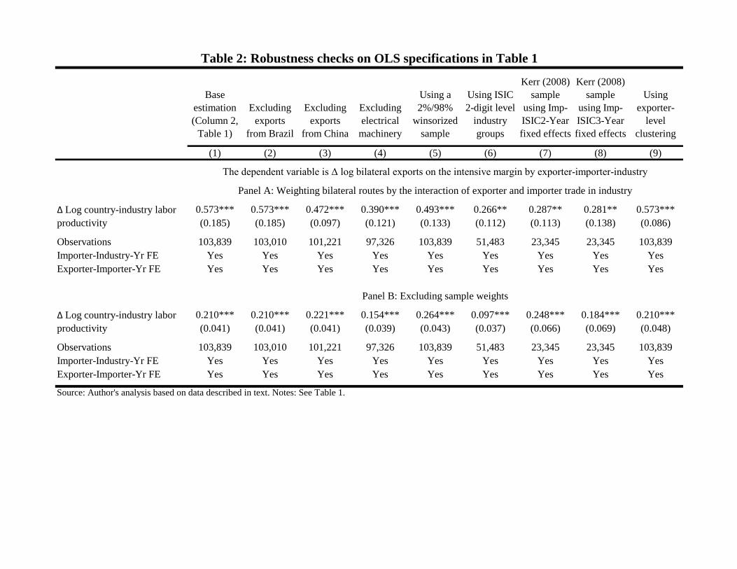
Table 2 provides robustness checks on the first-differenced estimates, which are the focus of the

remainder of this study. The first column repeats the core results from Column 2 of Table 1.

The next two columns show robustness to dropping Brazil and China. Brazil, of all included

countries, displays the most outlier behavior with respect to its productivity growth rates, likely

due to definitional changes, but Brazil’s exclusion does not affect the results. The results are

also similar when excluding China, which experienced substantial growth during the sample

period. It is generally worth noting that the 1980-1999 period pre-dates the very rapid take-off

of Chinese manufacturing exports after 2000 (Autor et al. 2013). Unreported tests consider other

candidates like Mexico, Germany, and Japan, and these tests, too, find the results very stable to

the sample composition, reflective in large part of the underlying exporter-importer-year fixed

effects.

Column 4 shows the results when excluding industry 383 (Machinery, electrical). The coeffi -

cient estimates are reduced in size by about 30% from Column 1, but they remain quite strong

and well-measured overall. The exclusion of industry 383 has the largest impact on the results

of the 26 industries in the sample, which is why it is reported. This importance is not very

surprising given the very rapid development of technology in this sector, its substantial diffusion

around the world, and its associated trade. On this dimension, the industry-year portion of the

importer-industry-year fixed effects play a very stabilizing role. Quantitatively similar results

are also found when excluding the Tobacco and Petroleum sectors (314, 353, 354). Column 5

shows that winsorizing the sample at the 2%/98% level delivers similar results, indicative that

outliers are not overly influencing the measured elasticities.

It was earlier noted that computational demands require that the main estimations employ

the ISIC2-level industry groups when preparing importer-industry-year fixed effects. Columns

6-8 test this choice in several ways. First, Column 6 shows that the results hold when estimating

the full model with ISIC2-based cells, so that the importer-industry-year fixed effects exactly

match the cell construction. The weaker variation reduces the coeffi cient estimates by half,

but the results remain statistically and economically important. Columns 7 and 8 alternatively

estimate the model using the sample from Kerr (2008) that focuses on a subset of the UNIDO

data in the 1985-1997 period. The Kerr (2008) sample is substantially smaller in size than

the present one, and so there is greater flexibility with respect to these fixed effect choices.

16

The choice of industry aggregation for the importer-industry-year fixed effects does not make a

material difference in this sample.10

Finally, Column 9 shows the results with exporter-level clustering. The labor productivity

and export development of industries within countries may be correlated with each other due to

the presence of general-purpose technologies, learning-by-doing (e.g., Irwin and Klenow 1994),

and similar factors, and Feenstra and Rose (2000) show how the export ranges of countries can

change over time in systematic ways across industries. Clustering at the exporter level allows for

greater covariance across industries in this regard, returning lower standard errors. Most papers

in this literature use robust standard errors on cross-sectional data, which would translate most

closely to bilateral-route clustering in a panel model. Unreported estimates consider bilateral-

route clustering and alternatively bootstrapped standard errors, and these standard errors are

smaller than those reported in Column 9.

Further extensions are contained in Tables S3 and S4. Interacting our core regressor with the

GDP/capita level of the exporter suggests that the OLS link between productivity and exports

is mainly through lower-income countries, suggestive of higher trade due to varieties among

developed economies. It is similar to the conclusion of Fieler (2011) that trade among advanced

economies links to product differentiation and variety (low θ), while trade among emerging

economies links more closely to fundamental productivity levels (higher θ). By contrast, there

is limited heterogeneity by country size or geographic distances, excepting the fact that the

growth in exports is not simply happening to bordering countries. Additional tests further

confirm that the observed role for technology within manufacturing is not due to specialized

factor accumulations and a Rybczynski effect. Under the Rybczynski effect, the accumulation

of skilled workers in country i shifts country i’s specialization towards manufacturing industries

that employ skilled labor more intensively than other factors. When incorporating country-

specific time trends for sub-groups of manufacturing industries according to their capital-labor

ratio, mean wage rate, and non-production worker share as evident in the United States, the

importance of technology’s importance is confirmed. Finally, there is limited adjustment on the

extensive margin of trade routes compared to the intensive margin adjustments.

10This extra check also has the advantage of linking the two studies closer together since the Kerr (2008) paperfocuses extensively on productivity growth due to technology transfer. Stability to the somewhat different datapreparation steps in Kerr (2008) is comforting.

17

3.3 Base IV Results

Table 3 presents the core IV results. The first column reports the first-stage estimates of how

∆ ln(Mkit) predicts∆ ln(zkit). The first-stage elasticity in Panel A is 0.6, suggesting a 10% increase

in the technology flow metric from the United States predicts a 6% increase in labor productivity

abroad at the exporter-industry level. The unweighted estimates in Panel B suggest a smaller

3% increase. While the second elasticity is lower, the instrument generally performs better in the

unweighted specifications due to its more precise measurement. The F statistics in Panels A and

B are 4.7 and 11.6, respectively. The sample weights in Panel A place greater emphasis on larger

and more advanced countries that have large export volumes (e.g., Germany, Japan). While this

framework finds a substantial response, the weighted dependency of this group on heterogeneous

technology transfer from the United States is noisier than in the unweighted estimations that

emphasize more developing and emerging countries.

The second column presents the reduced-form estimates where ∆ ln(Mkit) predicts ∆ ln(xkijt)

using a format similar to equation (3). In both panels, there is substantial reduced-form link of

technology flows to export volumes. The interquartile range in the reduced form, conditional on

the fixed effects, can account for around 6% of the interquartile range of export growth using a

0.8 coeffi cient estimate that sits in between Panels A and B.

The third column provides the second-stage estimates from equation (3) having used∆ ln(Mkit)

to predict ∆ ln(zkit). In Panel A’s estimation, the weighted elasticity is 1.6, suggesting a 16%

increase in export volumes for every 10% increase in labor productivity. In Panel B’s unweighted

estimation, the 10% increase in labor productivity is linked to a 24% increase in export volumes.

The second-stage elasticity in Panel B is larger than in Panel A, as the IV estimates provide the

reduced-form scaled up by the first-stage effects. Thus, even though the unweighted reduced-

form estimate in Column 2 is smaller than the weighted reduced-form estimate, this ordering

reverses once scaled-up by the first stages.

This study does not overly favor one set of estimates. The unweighted and unweighted

approaches both have merits and liabilities. Instead, the conclusion from this work is that the

instrumented elasticity is in the neighborhood of two. While it is impossible to differentiate

among the various reasons as to why the IV estimates are larger than the OLS estimates, a

very likely candidate is that OLS suffers from a substantial downward bias due to measurement

error in the labor productivity estimates, especially with the substantial differencing embedded

in equation (3). While it is likely that omitted factors or reverse causality influenced the OLS

18

estimations as well, these appear to have been second-order to the measurement issues.11

This instrumented θ elasticity is at the lower end of the estimates provided in the literature.

Costinot et al. (2012) is the closest comparison given their use of industry-level regressions of

productivity data and trade. Using a cross-sectional analysis of producer price data for OECD

countries in 1997, they derive their preferred estimate of 6.5, which is substantially larger than

this study’s estimate of about two. On the other hand, Costinot et al. (2012) derive a quite

similar elasticity of 2.7 when they consider labor productivity metrics, the metric considered

here. They too have IV estimates that are considerably larger than OLS estimates. More

broadly, Eaton and Kortum (2002) provide larger initial estimates of the θ elasticity, with a

preferred estimate in the range of eight. Simonovska and Waugh (2014a) revisit these results

with a new estimator and come to a preferred estimate of about four. Overall, this study’s

estimates are again lower than this connected work. The robustness checks described below find

θ estimates that continue in this ballpark, never exceeding four. Thus, this empirical approach

consistently derives θ estimates that are among the lowest in the literature, with some part of

this difference due to methodology but an important part being substantive in interpretation.

It is important to identify the dual meaning of the higher IV results compared to OLS

with respect to the θ parameter. In the Ricardian model, a higher θ parameter corresponds

to a reduced scope for intra-industry trade due to comparative advantages across varieties.

IV estimations thus suggest that OLS specifications overestimate the scope for intra-industry

trade because they understate the link between country-industry productivity improvements

and their associated export volumes. Both impetuses can be connected to Ricardian theories of

comparative advantage for trade, but the role of the structural θ parameter needs to be carefully

delineated. This partitioning can also have important consequences for views of development

and export success. Compared to OLS, the IV results shift more emphasis towards fundamental

country-industry productivity improvements rather than intra-industry varieties; yet, on the

whole, the overall work in this paper with emerging economies provides more support for intra-

industry varieties than typically found in the Ricardian literature that has focused mostly on

OECD trade flows (as evidenced by the lower θ estimates compared to prior studies).

These estimates are significant in terms of their potential economic importance and explana-

11Costinot et al. (2012) adjust export volumes for trade openness using the import penetration ratio for acountry-industry (to link observed productivity to "fundamental productivity"). The estimates are very similarwhen undertaking this approach, being 1.163 (0.457) and 2.513 (1.138) for weighted and unweighted specifica-tions, respectively. The unadjusted and adjusted first differences have a 0.93 correlation. This approach is notadopted for the main estimations due to worries about mismeasurement in the import penetration ratio whencombining UNIDO and WTF data.

19

tory power. Using an elasticity of two, the interquartile range of country-level labor productivity

growth, conditional on fixed effects, can explain up to 35% and 39% of the interquartile range

in conditional export growth levels using unweighted and weighted specifications, respectively.

3.4 Extended IV Results

The online supplement provides many robustness checks on these IV estimations in Tables S5-

S8b. The results are robust to the various specification checks conducted in Table 2. Moreover,

dynamic estimations find lagged productivity growth estimators consistently stronger than con-

temporaneous productivity growth estimators, providing comfort in the estimation design and

the proposed causal direction of the results. The IV is further analyzed when 1) considering

variations on the city-industry technology trend terms and cross-sectional distributions used to

weight US cities for the development of Mkit, 2) sample composition exercises that aggressively

test for data quality and reverse causality concerns, and 3) direct inclusion of ethnic patenting

in the United States as a control. The online supplement also contains an extended discussion

of the identification achieved in this study and its limitations. In the end, the paper is able to

make substantial progress towards causal identification in a Ricardian model, beginning with the

panel estimation approach and extending through many IV approaches. This effort remains in-

complete, however, and it is hoped that future work both identifies natural experiment settings

to test these arguments and also identifies other forms/impetuses for heterogeneous technol-

ogy transfer that can provide identification in a setting that focuses on large country-industry

samples like this one.

4 Conclusions

While the principle of Ricardian technology differences as a source of trade is well established

in the theory of international economics, empirical evaluations of its importance are relatively

rare due to the diffi culty of quantifying and isolating technology differences. This study exploits

heterogeneous technology diffusion from the United States through ethnic migrant networks to

make additional headway. Estimations find bilateral manufacturing exports respond positively

to growth in observable measures of comparative advantages. Ricardian technology differences

are an important determinant of trade in longitudinal changes, in addition to their cross-sectional

role discussed earlier.

Leamer and Levinsohn (1995) argue that trade models should be taken with a grain of salt

20

and applied in contexts for which they are appropriate. This is certainly true when interpret-

ing these results. The estimating frameworks have specifically sought to remove trade resulting

from factor endowments, increasing returns, consumer preferences, etc. rather than test against

them. Moreover, manufacturing exports are likely more sensitive to patentable technology im-

provements than the average sector, and the empirical reach of the constructed dataset to include

emerging economies like China and India heightens this sensitivity. Further research is needed

to generalize technology’s role to a broader set of industrial sectors and environments.

Beyond quantifying the link between technology and trade for manufacturing, this paper also

serves as input into research regarding the benefits and costs of emigration to the United States

for the migrants’home countries (i.e., the "brain drain" or "brain gain" debate). While focusing

on the Ricardian model and its parameters, the paper establishes that the technology transfers

from overseas migrants are strong enough to meaningfully promote exports. Care should be

taken to not overly interpret these findings as strong evidence of a big gain from migration.

The paper does not seek to establish a clear counterfactual in the context of immigration from

the source countries’point of view (e.g., Agrawal et al. 2011). As such, the positive export

elasticities due to US heterogeneous technology diffusion do not constitute welfare statements

relative to other scenarios. Future research needs to examine these welfare implications further.

ReferencesAcemoglu, Daron, and Jaume Ventura, "The World Income Distribution", Quarterly Journal ofEconomics, 117:2 (2002), 659-694.

Acemoglu, Daron, and Fabrizio Zilibotti, "Productivity Differences", Quarterly Journal of Eco-nomics, 116:2 (2001), 563-606.

Agrawal, Ajay, Devesh Kapur, John McHale, and Alexander Oettl, "Brain Drain or Brain Bank?The Impact of Skilled Emigration on Poor-Country Innovation", Journal of Urban Economics,69:1 (2011), 43-55.

Alcacer, Juan, andWilbur Chung, "Location Strategies and Knowledge Spillovers",ManagementScience, 53:5 (2007), 760-776.

Alvarez, Fernando, and Robert Lucas, "General Equilibrium Analysis of the Eaton-KortumModel of International Trade", Journal of Monetary Economics, 54 (2007), 1726-1768.

Antweiler, Werner, and Daniel Trefler, "Increasing Returns to Scale and All That: A View FromTrade", American Economic Review, 92 (2002), 93-119.

Autor, David, David Dorn, and Gordon Hanson, "The China Syndrome: Local Labor MarketEffects of Import Competition in the United States", American Economic Review, 103:6 (2013),2121-2168.Bahar, Dany, and Hillel Rapoport, "Migration, Knowledge Diffusion, and the ComparativeAdvantages of Nations", Economic Journal, forthcoming (2016).

Baxter, Marianne, "Fiscal Policy, Specialization, and Trade in the Two-Sector Model: TheReturn of Ricardo?", Journal of Political Economy, 100:4 (1992), 713-744.

21

Bo, Chen, and David Jacks, "Trade, Variety and Immigration", Economic Letters (2012), 243-246.Bombardini, Matilde, Chris Kurz, and Peter Morrow, "Ricardian Trade and the Impact ofDomestic Competition on Export Performance", Canadian Journal of Economics, 45:2 (2012),585-612.Caliendo, Lorenzo, and Fernando Parro, "Estimates of the Trade andWelfare Effects of NAFTA",Review of Economic Studies, 82:1 (2015), 1-44.

Chor, Davin, "Unpacking Sources of Comparative Advantage: A Quantitative Approach", Jour-nal of International Economics, 82 (2010), 152-167.

Cohen, Lauren, Umit Gurun, and Christopher Malloy, "Resident Networks and Firm Trade",Journal of Finance, 6 (2016), 63-91.

Costinot, Arnaud, "An Elementary Theory of Comparative Advantage", Econometrica, 77:4(2009), 1165-1192.

Costinot, Arnaud, and Andres Rodriguez-Clare, "Trade with Numbers: Quantifying the Conse-quences of Globalization", in Handbook of International Economics Volume 4 (Elsevier, 2014),197-261.Costinot, Arnaud, and David Donaldson, "Ricardo’s Theory of Comparative Advantage: OldIdea, New Evidence", American Economic Review Papers and Proceedings, 102:3 (2012), 453-458.Costinot, Arnaud, David Donaldson, and Ivana Komunjer, "What Goods Do Countries Trade?New Ricardian Predictions", Review of Economic Studies, 79:2 (2012), 581-608.

Costinot, Arnaud, and Jonathan Vogel, "Beyond Ricardo: Assignment Models in InternationalTrade", Annual Review of Economics, 7 (2015), 31-62.

Daruich, Diego, William Easterly, and Ariell Reschef, "The Surprising Instability of ExportSpecializations", NBER Working Paper 22869 (2016).

Davis, Donald, and David Weinstein, "An Account of Global Factor Trade", American EconomicReview, 91:5 (2001), 1423-1453.

Davis, Donald, and DavidWeinstein, "Technological Superiority and the Losses fromMigration",NBER Working Paper 8971 (2002).

di Giovanni, Julian, Andrei Levchenko, and Francesco Ortega, "A Global View of Cross-BorderMigration", Journal of the European Economic Association, 31:1 (2015), 168-202.

Dornbusch, Rudiger, Stanley Fischer, and Paul Samuelson, "Comparative Advantage, Trade andPayments in a Ricardian Model with a Continuum of Goods", American Economic Review, 67:5(1977), 823-839.

Eaton, Jonathan, and Samuel Kortum, "International Technology Diffusion: Theory and Mea-surement", International Economic Review, 40:3 (1999), 537-570.

Eaton, Jonathan, and Samuel Kortum, "Technology, Geography, and Trade", Econometrica,70:5 (2002), 1741-1779.

Feenstra, Robert, Robert Lipsey, Haiyan Deng, Alyson Ma, and Hengyong Mo, "World TradeFlows: 1962-2000", NBER Working Paper 11040 (2005).

Feenstra, Robert, and Andrew Rose, "Putting Things in Order: Trade Dynamics and ProductCycles", Review of Economics and Statistics, 82:3 (2000), 369-382.

Fieler, Ana Cecilia, "Nonhomotheticity and Bilateral Export Trade: Evidence and a QuantitativeExplanation", Econometrica, 79:4 (2011), 1069-1101.

22

Foley, C. Fritz and William Kerr, "Ethnic Innovation and U.S. Multinational Firm Activity",Management Science, 59:7 (2013), 1529-1544.

Golub, Stephen, and Chang-Tai Hsieh, "Classical Ricardian Theory of Comparative AdvantageRevisited", Review of International Economics, 8:2 (2000), 221-234.

Gould, David, "Immigrant Links to the Home Country: Empirical Implications for US BilateralTrade Flows", Review of Economics and Statistics, 76:3 (1994), 500-518.

Hakobyan, Shushanik, and John McLaren, "Looking for Local Labor Market Effects of NAFTA",Review of Economics and Statistics, 98:4 (2016), 728-741.

Hall, Bronwyn, Adam Jaffe, and Manuel Trajtenberg, "The NBER Patent Citation Data File:Lessons, Insights and Methodological Tools", NBER Working Paper 8498 (2001).

Harrigan, James, "Technology, Factor Supplies, and International Specialization: Estimatingthe Neoclassical Model", American Economic Review, 87:4 (1997), 475-494.

Head, Keith, and John Reis, "Immigration and Trade Creation: Econometric Evidence fromCanada", Canadian Journal of Economics, 31:1 (1998), 47-62.

Helpman, Elhanan, and Paul Krugman, Market Structure and Foreign Trade (Cambridge, MA:MIT Press, 1985).

Hummels, David, and Peter Klenow, "The Variety and Quality of a Nation’s Exports", AmericanEconomic Review, 95:3 (2005), 704-723.

Hunt, Jennifer, and Marjolaine Gauthier-Loiselle, "How Much Does Immigration Boost Innova-tion?", American Economic Journal: Macroeconomics, 2 (2010), 31-56.

Hunter, Linda, "The Contribution of Non-Homothetic Preferences to Trade", Journal of Inter-national Economics, 30:3 (1991), 345-358.

Hunter, Linda, and James Markusen, "Per Capita Income as a Determinant of Trade", in RobertFeenstra, ed., Empirical Methods for International Trade (Cambridge, MA: MIT Press, 1988).

Irwin, Douglas, and Peter Klenow, "Learning by Doing Spillovers in the Semiconductor Indus-try", Journal of Political Economy, 102 (1994), 1200-1227.

Keller, Wolfgang, "Geographic Localization of International Technology Diffusion", AmericanEconomic Review, 92:1 (2002), 120-142.

Kerr, William, "Ethnic Scientific Communities and International Technology Diffusion", Reviewof Economics and Statistics, 90:3 (2008), 518-537.

Kerr, William, "The Ethnic Composition of US Inventors", HBS Working Paper 08-006 (2007).

Kerr, William, "The Role of Immigrant Scientists and Entrepreneurs in International TechnologyTransfer", MIT Ph.D. Dissertation (2005).

Kerr, William, and William Lincoln, "The Supply Side of Innovation: H-1B Visa Reforms andUS Ethnic Invention", Journal of Labor Economics, 28:3 (2010), 473-508.

Kovak, Brian, "Regional Effects of Trade Reform: What is the Correct Measure of Liberaliza-tion?", American Economic Review, 103:5 (2013), 1960-1976.

Kugler, Maurice, and Hillel Rapoport, "International Labor and Capital Flows: Complementsor Substitutes?", Economics Letters, 92.2 (2007), 155-162.

Leamer, Edward, and James Levinsohn, "International Trade Theory: The Evidence", Handbookof International Economics, 3 (1995), 1339-1394.

Levchenko, Andrei, and Jing Zhang, "Ricardian Productivity Differences and the Gains fromTrade", European Economic Review, 65 (2014), 45-65.

23

MacDougall, G.D.A., "British and American Exports: A Study Suggested by the Theory ofComparative Costs. Part I", Economic Journal, 61:244 (1951), 697-724.

MacDougall, G.D.A., "British and American Exports: A Study Suggested by the Theory ofComparative Costs. Part II", Economic Journal, 62:247 (1952), 487-521.

Morrow, Peter, "Ricardian-Heckscher-Ohlin Comparative Advantage: Theory and Evidence",Journal of International Economics, 82:2 (2010), 137-151.

Peri, Giovanni, Kevin Shih, and Chad Sparber, "STEM Workers, H1B Visas and Productivityin US Cities", Journal of Labor Economics, 33:S1 (2015), S225-S255.

Rauch, James, "Business and Social Networks in International Trade", Journal of EconomicLiterature, 39 (2001), 1177-1203.

Rauch, James, and Vitor Trindade, "Ethnic Chinese Networks in International Trade", Reviewof Economics and Statistics, 84:1 (2002), 116-130.

Ricardo, David, On the Principles of Political Economy and Taxation (London, UK: John Mur-ray, 1817).

Saxenian, AnnaLee, with Yasuyuki Motoyama and Xiaohong Quan, Local and Global Networksof Immigrant Professionals in Silicon Valley (San Francisco, CA: Public Policy Institute ofCalifornia, 2002).

Saxenian, AnnaLee, The New Argonauts (Cambridge, MA: Harvard University Press, 2006).

Shikher, Serge, "Putting Industries into the Eaton—Kortum Model", Journal of InternationalTrade & Economic Development, 21:6 (2012), 807-837.

Simonovska, Ina, and Michael Waugh, "The Elasticities of Trade: Estimates and Evidence",Journal of International Economics, 92:1 (2014a), 34-50.

Simonovska, Ina, and Michael Waugh, "Trade Models, Trade Elasticities, and the Gains fromTrade", NBER Working Paper 20495 (2014b).

Stern, Robert, "British and American Productivity and Comparative Costs in InternationalTrade", Oxford Economic Papers, 14:3 (1962), 275-296.

Wilson, Charles, "On the General Structure of Ricardian Models with a Continuum of Goods:Applications to Growth, TariffTheory, and Technical Change", Econometrica, 48:7 (1980), 1675-1702.

24

Between estimation FD estimation

(1) (2)

DV: Log bilateral exports DV: Δ Log bilateral exports

Log country-industry labor 0.640***

productivity (0.242)

Δ Log country-industry labor 0.573***

productivity (0.185)

Observations 149,547 103,839

Importer-Industry-Yr FE Yes Yes

Exporter-Importer-Yr FE Yes Yes

DV: Log bilateral exports DV: Δ Log bilateral exports

Log country-industry labor 0.361***

productivity (0.091)

Δ Log country-industry labor 0.210***

productivity (0.041)

Observations 149,547 103,839

Importer-Industry-Yr FE Yes Yes

Exporter-Importer-Yr FE Yes Yes

Table 1: OLS estimations of labor productivity and exports

Panel A: Weighting bilateral routes by the interaction of exporter and

importer trade in industry (summed across all bilateral routes)

Panel B: Excluding sample weights

Source: Author's analysis based on data described in text. Notes: Panel estimations consider manufacturing exports

taken from the WTF database. Data are organized by exporter-importer-industry-year. Industries are defined at the

three-digit level of the ISIC Revision 2 system. Annual data are collapsed into five-year groupings beginning with 1980-

1984 and extending to 1995-1999. The dependent variable in Column 1 is the log mean nominal value (US$) of

bilateral exports for the five years; the dependent variable in Column 2 is the change in log exports from the prior

period. The intensive margin sample is restricted to exporter-importer-industry groupings with exports exceeding

$100k in every year. The $100k threshold is chosen due to WTF data collection procedures discussed in the text. Labor

productivity from the UNIDO database measures comparative advantages. Column 1 estimates Ricardian elasticities

using both within-panel variation and variation between industries of a country. Column 2 estimates Ricardian

elasticities using only variation within panels. Estimations in Panel A weight bilateral routes by the interaction of total

exporter and importer trade in industry; estimations in Panel B are unweighted. Estimations cluster standard errors by

exporter-industry. Importer-Industry-Yr FE are defined at the two-digit level of the ISIC system. *, **, *** denote

statistical significance at the 10%, 5%, and 1% levels, respectively.

Base

estimation

(Column 2,

Table 1)

Excluding

exports

from Brazil

Excluding

exports

from China

Excluding

electrical

machinery

Using a

2%/98%

winsorized

sample

Using ISIC

2-digit level

industry

groups

Kerr (2008)

sample

using Imp-

ISIC2-Year

fixed effects

Kerr (2008)

sample

using Imp-

ISIC3-Year

fixed effects

Using

exporter-

level

clustering

(1) (2) (3) (4) (5) (6) (7) (8) (9)

Δ Log country-industry labor 0.573*** 0.573*** 0.472*** 0.390*** 0.493*** 0.266** 0.287** 0.281** 0.573***

productivity (0.185) (0.185) (0.097) (0.121) (0.133) (0.112) (0.113) (0.138) (0.086)

Observations 103,839 103,010 101,221 97,326 103,839 51,483 23,345 23,345 103,839

Importer-Industry-Yr FE Yes Yes Yes Yes Yes Yes Yes Yes Yes

Exporter-Importer-Yr FE Yes Yes Yes Yes Yes Yes Yes Yes Yes

Δ Log country-industry labor 0.210*** 0.210*** 0.221*** 0.154*** 0.264*** 0.097*** 0.248*** 0.184*** 0.210***

productivity (0.041) (0.041) (0.041) (0.039) (0.043) (0.037) (0.066) (0.069) (0.048)

Observations 103,839 103,010 101,221 97,326 103,839 51,483 23,345 23,345 103,839

Importer-Industry-Yr FE Yes Yes Yes Yes Yes Yes Yes Yes Yes

Exporter-Importer-Yr FE Yes Yes Yes Yes Yes Yes Yes Yes Yes

Table 2: Robustness checks on OLS specifications in Table 1

Panel A: Weighting bilateral routes by the interaction of exporter and importer trade in industry

Panel B: Excluding sample weights

Source: Author's analysis based on data described in text. Notes: See Table 1.

The dependent variable is Δ log bilateral exports on the intensive margin by exporter-importer-industry

First-stage estimation Reduced-form estimation IV estimation

(1) (2) (3)

DV: Δ Log country-

industry labor productivity

DV: Δ Log bilateral

exports

DV: Δ Log bilateral

exports

Δ Log estimator for technology 0.589** 0.938***

flows from the United States (0.272) (0.298)

Δ Log country-industry labor 1.592**

productivity (0.637)

Observations 103,839 103,839 103,839

Importer-Industry-Yr FE Yes Yes Yes

Exporter-Importer-Yr FE Yes Yes Yes

DV: Δ Log country-

industry labor productivity

DV: Δ Log bilateral

exports

DV: Δ Log bilateral

exports

Δ Log estimator for technology 0.267*** 0.648***

flows from the United States (0.078) (0.112)

Δ Log country-industry labor 2.429***

productivity (0.791)

Observations 103,839 103,839 103,839

Importer-Industry-Yr FE Yes Yes Yes

Exporter-Importer-Yr FE Yes Yes Yes

Table 3: IV estimations of labor productivity and exports

Panel A: Weighting bilateral routes by the interaction of exporter and importer

trade in industry

Panel B: Excluding sample weights

Source: Author's analysis based on data described in text. Notes: See Table 1. The instrument combines panel variation on the

development of new technologies across US cities during the 1975-2000 period with historical settlement patterns for migrants and

their ancestors from countries that are recorded in the 1980 Census of Populations. The F statistics in Panels A and B are 4.7 and

11.6, respectively.

Online Supplement forHeterogeneous Technology Diffusion and Ricardian Trade Patterns

1 Additional Literature

Recent research quantifies the role of international labor mobility in ethnic technology exchanges

(e.g., Saxenian 2006, Kapur and McHale 2005, Obukhova 2008, 2009, Nanda and Khanna

2010). Related unpublished work includes Papageorgiou and Spilimbergo (2008) and Kugler

and Rapoport (2012). Other sources of heterogeneous technology frontiers are geographic dis-

tances to major R&D nations (e.g., Keller 2002), the innovative efforts of trading partners (e.g.,

Grossman and Helpman 1991, Coe and Helpman 1995, Coe et al. 1997), or international patent-

ing decisions (e.g., Eaton and Kortum 1999). Keller (2004) reviews the technology transfer

literature.

2 Costinot et al. (2012). Model

This theoretical framework derives from Costinot et al. (2012). A world economy is comprised

of I countries and K industries or goods. Labor is the sole factor of production and there

are constant returns to scale in the production of each good. Labor is perfectly mobile across

industries and immobile across countries. Li and wi are the number of workers and the wage

rate in country i, respectively. Consumers consume their full wages in each period. Accordingly,

time subscripts are omitted until the estimating equation is introduced. Countries are free to

produce or trade all goods. Each good k ∈ K has an infinite number of varieties indexed by

ω ∈ Ω ≡ [1, . . . ,+∞]. zki (ω) represents the number of units of the ωth variety of good k that

can be produced with one unit of labor in country i.

Following Eaton and Kortum (2002), zki (ω) is a random variable drawn independently for

each triplet (i, k, ω) from a Fréchet distribution,

F ki (z) = exp[−(z/zki )−θ], for all z ≥ 0, (1)

where zki > 0 and θ > 1. Thus, technological differences across countries and industries depend

on two parameters, zki and θ. The first parameter zki captures the fundamental productivity

of country i in industry k, which affects the productivity of all producers (e.g., institutions,

climate). For each industry, the cross-country variation of this zki parameter governs the cross-

country variation in relative labor productivity that sits at the core of the standard Ricardian

1

model. A larger zki raises the absolute advantage for trade for exporter i in industry k. The second

parameter θ models the intra-industry heterogeneity that exists due to the scope for idiosyncratic

differences in technological know-how across varieties. This variation is the same in all countries

and industries, and θ parameterizes the impact of changes in fundamental productivity levels

zki on aggregate trade flows. A larger θ implies a tighter distribution that limits the scope for

comparative advantage across nations.

Trade frictions have iceberg costs such that for each unit of good k shipped from exporter i

to importer j, only 1/dkij ≤ 1 units arrive, with dkii = 1 and dkil ≤ dkij · dkjl for any third country lto rule out cross-country arbitrage opportunities. Perfect competition in markets and constant

returns to scale in production imply that the price pkj (ω) paid by buyers of variety ω of good k

in any country j is

pkj (ω) = mini∈I

[ckij(ω)], (2)

where ckij(ω) = (dkij · wi)/zki (ω) is the cost of producing and delivering one unit of this variety

from country i to country j. For each variety ω of good k, buyers in country j select the best

price available from around the world. An increase in country i’s effi ciency for good j lowers the

price it must charge.

Representative consumers in each country have a two-tier utility function. The upper tier is

Cobb-Douglas, and the preference parameter αkj measures the share of expenditure on varieties

from industry k in country j. The lower tier is constant elasticity of substitution (CES), and

σkj is the elasticity of substitution between varieties. Accordingly, expenditures are such that in

any importer j, total expenditure on variety ω of good k is

xkj (ω) = [pkj (ω)/pkj ]1−σkj · αkjwjLj, (3)

where 0 ≤ αkj ≤ 1, σkj < 1+θ, and pkj ≡[∑

ω′∈Ω pkj (ω

′)1−σkj]1/(1−σkj )

. The restriction σkj < 1+θ is

a technical assumption that guarantees the existence of a well-defined CES price index pkj . The

consumer price index in country j is pj ≡∏K

k=1(pkj )αkj .

The value of total exports from exporter i to importer j in industry k is xkij ≡∑

ω′∈Ωkijxkj (ω

′),

where Ωkij denotes the set of varieties exported. The share of exports in importer j and industry

k from country i is πkij ≡ xkij/∑I

i′=1 xki′j. With this model structure, the bilateral exports from

exporter i to importer j in industry k is

xkij =(wid

kij/z

ki )−θ∑I

i′=1(wi′dki′j/zki′)−θ· αkjwjLj, (4)

2

which has an intuitive interpretation that closely connects to a similar expression in Eaton and

Kortum (2002). The righthand terms express the overall economic size of the importer j and its

preferences over goods. The lefthand fraction describes the extent to which the exporter is the

lowest cost producer of the good, taking into account delivery costs, production costs, technology

levels, and the underlying heterogeneity in varieties for countries. Under assumptions of balanced

trade, the relatives wages around the world can further be determined.

Costinot et al. (2012) show that equation (4) provides the foundation for estimating an

econometric equation of the form shown in specification (1) of main text: ln(xkij)

= δij + δkj +

θ ln(zki ) + εkij, where xkij represents "corrected" trade flows that adjust for country openness.

Similarly, zki represents observed productivity, given that not every country produces every good

as it can import goods from other countries. δij and δkj are vectors of exporter-importer and

importer-industry fixed effects. Comparing these equations shows the basic function of these

fixed effects. The importer-industry fixed effects control for the righthand terms about the

importer and its preferences over goods. Importer-industry fixed effects also account for the

denominator of the lefthand fraction, given that it is a worldwide aggregate for an industry. The

exporter-importer fixed effects capture the numerator’s terms, which emphasize cost levels in

the exporter and distances between the two countries. Under the assumption that the delivery

cost term dkij in the numerator can be expressed in proportionate terms over these two vectors

of fixed effects (e.g., dkij = dij · dkj ), specification (1) of main text provides an unbiased estimateof the θ parameter. An alternative assumption is that the residual differences in delivery costs

after controlling for these vectors of fixed effects are uncorrelated with the focal productivity

level zki .

3 Extended Data Development

3.1 Labor Productivity Data

The UNIDO collects industry-level manufacturing statistics for The International Yearbook of

Industrial Statistics and specialized publications on topics like development and competition.

Researchers at the UNIDO supplement the data resources of the OECD with national records

for non-OECD members, creating a unique global resource. The UNIDO’s stated objective

is the compilation of internationally comparable and internally consistent series (e.g., variable

definitions, accounting units, collection procedures).

Table S1a describes the 88 exporting countries included. Column 2 provides a count of the

3

number of periods the country is included in after the first difference is taken, with a maximum

of three changes. Column 3 documents the count of bilateral route observations included at

the exporter-importer-industry level for the intensive-margin estimations. The total observation

count is 103,839 intensive-margin changes for an exporter-importer-industry. Countries differ

in their observation counts, even if observed for the same number of periods, due to variations

in their industry-level reporting in the UNIDO database and minimum requirements for export

volumes discussed below.

Column 4 documents the average manufacturing productivity levels for countries, expressed

in US dollars. While direct comparisons across countries are limited with an unbalanced panel,

productivity differences between industrialized countries and developing nations are clearly evi-

dent. Oil-producing countries (e.g., Kuwait, Norway) have the highest average labor productiv-

ity levels, with Ireland, Japan and Singapore among the highest when excluding oil producers.

Afghanistan, Bangladesh, and Myanmar are among the lowest levels recorded. A small num-

ber of country-industry observations with under ten employees or very problematic data are

excluded. Column 5 documents the mean growth rate in labor productivity for each country

over its observations. These growth rates are five-year differences, with outliers winsorized at

their 2% and 98% levels for reporting. Hong Kong, Myanmar, Peru, and Syria have the highest

growth rates, while the Dominican Republic, Tanzania, and Romania show the sharpest declines.

Table S1b provides similar statistics for the 26 industries, aggregating over countries. In-

dustry 353 (Petroleum refineries) has the highest average labor productivity, while industry 322

(Wearing apparel, except footwear) has the lowest. Productivity growth is strongest in industries

382 and 383 (Machinery, except electrical, and Machinery, electric). Productivity growth rates

are lowest in industry 323 (Leather products) and industry 361 (Pottery, china, earthenware).

Most Ricardian models suggest using labor productivity to measure comparative advantage.

This is fortunate in that manufacturing output and employment data are among the most avail-

able metrics for the broad grouping of countries under study. Labor is typically the only factor

of production in Ricardian models, so a natural extension might be total factor productivity that

also allows for capital accumulation as well. Unfortunately, capital data at the country-industry

level for this sample is too sparse to be of benefit in a panel study. An earlier version of this

paper presents results using output to measure industrial specialization.

4

3.2 Export Volumes

Columns 6-8 of Tables S1a and S1b describe the WTF data. These descriptives focus on the

intensive-margin estimations that require exporter-importer-industry observations maintain the

minimum threshold of trade volume. Columns 6 and 7 provide comparable statistics about the

mean export levels and growth rates for included routes. Germany and Japan have the highest

average volumes, and Nicaragua and El Salvador have the lowest average volumes. Export growth

rates are strongest in Nicaragua, Congo, and Costa Rica, and they are lowest in Guatemala and

Zimbabwe. From an industry perspective, trade volumes have the highest average values in

industries 382-384 (Machinery and Transportation equipment), and the lowest average volumes

are observed in industry 361 (Pottery, china, earthenware). Industry 383 (Machinery, electric)

has the highest growth rate, while industries 353 (Petroleum refineries) and 371 (Iron and steel)

have the lowest.

Column 8 of Table S1a documents the share of total WTF exports for countries that are

included in this sample. The main reasons why exports are not included are lack of corresponding

UNIDO labor productivity estimates or that the exports are going to the United States. This

sample accounts for 78% of exports to destinations other than United States from these countries

(about 63% if exports to the United States are included in the denominator). Column 8 of Table

S1b provides comparable data for industries. The sample accounts for 69% of exports in these

industries to destinations other than United States. This share is lower than 78% due to the

inclusion of exporters not captured in Table S1a. Much of the decline on the industry side comes

through limited representation of major petroleum producers.

Price deflators are not available for this sample (exports or labor productivity data). To the

extent that exporter-industry-year deflators are comprised of exporter-year, industry-year, and

exporter-industry components, the fixed effects and first differencing strategy will control for

them automatically. Residual exporter-industry-year trends could bias OLS estimations. The

IV estimations will overcome any such OLS biases due to deflators.

As a final note, a break exists in WTF data collection procedures at 1984. This break

does not have a significant impact on ISIC3-level export volumes, and the results are robust to

dropping the initial period.

5

3.3 US Historical Settlement Patterns

Columns 9 and 10 of Table S1a provide the largest cities for each country’s ancestry population.

Due to their large overall size and high immigration shares, cities like New York, Los Angeles,

and Miami appear frequently. Nonetheless, there is substantial heterogeneity. East and West

Coast cities are more likely to link respectively to European and Asian ancestries, for example,

while southern parts of the United States link more to Latin American ancestries. The migration

from Nordic countries to the mid-west is evident (e.g., Finland’s presence in Minnesota).

Robustness checks use the spatial distributions present in the 1990 Census of Populations.

These patterns are constructed from the 5% sample in a manner that parallels the 1980 distri-

bution.

3.4 US Patenting Data

The addresses listed on inventor records are used to group patents to the cities identified in the

1980 census. This procedure uses city lists collected from the Offi ce of Social and Economic

Data Analysis at the University of Missouri, with a matching rate of 99%. Manual recoding

further ensures that all patents with more than 100 citations and all city names with more than

100 patents are identified. Some smaller metropolitan areas identified in the patent data are

excluded since they do not link to places identified in the 1980 census. Only patents with all

inventors living in the United States at the time of their patent application are included, and

multiple inventors are discounted so that each patent receives the same weight when measuring

inventor populations.

Second, the USPTO issues patents by technology categories rather than by industries. The

work of Johnson (1999), Silverman (1999), and Kerr (2008) develops concordances that link

the USPTO classes to ISIC3 industries in which new inventions are manufactured or used.

The main estimations focus on industry-of-use, affording a composite view of the technological

opportunity developed for an industry. Studies of advanced economies find accounting for these

inter-industry R&D flows important (e.g., Scherer 1984, Keller 2002b). Estimations using the

alternative categorization of technologies to industry of manufacturer are also presented below.

Cohen (2011) discusses the larger literature on industry-level mappings and evidence regarding

patents, R&D, and productivity.

With respect to ethnic name matching, Kerr (2007) documents specific algorithms, lists

frequent ethnic names, and provides extensive descriptive statistics. This paper also discusses

6

quality assurance exercises performed. For example, the ethnic-name database can be applied

to foreign patents registered with the USPTO. The ethnic-name database assigns ethnicities to

98% of foreign records. Moreover, estimated inventor compositions are quite reasonable– for

example, approximately 90% of inventors filing from Chinese countries and regions are classified

as ethnically Chinese.

The developed approach, in combination with the interactions embedded in model Mkit out-

lined in the main text, has the subtler advantage of allowing the construction of instruments

for many more countries and their ancestry groups than what one can directly identify through

inventor names, either due to lack of names for some countries (e.g., Ethiopia, Oman) or due

to extensive name overlap among countries within an ethnic group (e.g., most of Latin Amer-

ica sharing Hispanic names). The instrument also has only non-zero predicted changes for

country-industries due to its summation over cities and the connection to Anglo-Saxon technol-

ogy development in cities.

The Costinot et al. (2012) model dictates the inclusion of importer-industry-year fixed effects

δkjt in the first-differenced specification for structural reasons such as country preferences. Two

other rationales exist for having at least industry-year fixed effects due to the data development

depicted. First, the US technology frontier is taken as exogenous in the IV model, and the

identification of the θ parameter should thus be independent of the pace of US technology

expansion in different industries. A second methodological rationale stems from the US patent

process. US patent grants have increased dramatically since the early 1980s. While several

factors lie behind this increase, it is clear that USPTO grant rates grew faster than the underlying

growth of US scientific personnel and innovation can explain. Moreover, differences in grant rates

exist across industries. The fixed effects account for these secular changes in the underlying

patenting productivity.1

4 Extended OLS Empirical Results

Table S3 considers several extensions of Table 1 to characterize heterogeneity in the sample.

Column 2 interacts the regressor with the GDP/capita level of the exporter, broken down into

quintiles. Interestingly, the OLS link between base productivity and exports is mainly coming

off of the lower-income countries, suggestive of higher trade due to varieties among developed

economies. This may be due to the greater potential for within-country productivity dispersion

1For example, Griliches (1990), Kortum and Lerner (2000), Kim and Marschke (2004), Hall (2005), Branstetterand Ogura (2005), Jaffe and Lerner (2005), and Lemley and Sampat (2008).

7

in the sample of developing and emerging economies, their more rapid productivity development

over the 1980-1999 period, and similar factors. It is similar to the conclusion of Fieler (2011) that

trade among advanced economies links to product differentiation and variety (low θ), while trade

among emerging economies links more closely to fundamental productivity levels (higher θ).2 By

contrast, Column 3 finds very little difference across countries of different sizes. Columns 4 and

5 also show very little connection of export growth to geographic distances, excepting the fact

that the growth in exports is not simply happening to bordering countries. These extensions

suggest that spatial distance is a second-order factor in shaping where export growth occurs

following technology expansion.

In contrast to the Ricardian framework, Heckscher-Ohlin-Vanek (HOV) models describe trade

as resulting from factor differences across countries (e.g., labor, capital, natural resources). In

the above model, technology is the only channel promoting export growth due to identical

factor endowments and no intertemporal factor accumulation. During the period studied, some

countries experienced significant growth in their skilled labor forces and physical capital stocks,

as well as their technology sets, and the former could lead to growth in manufacturing exports

due to the Rybczynski effect. Capital accumulation is particularly noted in rapid advances

made by several East Asian economies (e.g., Young 1992, 1995; Ventura 1997). The inclusion

of exporter-importer-year fixed effects suggests that a Rybczynski effect for the manufacturing

sector as a whole is not responsible for the observed trade patterns. Columns 6-8 provide

additional evidence that the observed role for technology within manufacturing is not due to

specialized factor accumulations.3

The intuition behind the proposed test is straightforward. Under the Rybczynski effect, the

accumulation of skilled workers in country i shifts country i’s specialization towards manufac-

turing industries that employ skilled labor more intensively than other factors. By grouping

manufacturing industries by their skilled-labor intensities, tests examine if technology’s impor-

tance is preserved after time trends are removed for these industry groups within each country.

These time trends are included in addition to the fixed effects listed at the bottom of the table.

To illustrate, the computer and pharmaceutical industries are both highly skill intensive. A

general Rybczynski effect due to skilled worker accumulation in China would favor specializa-

2These interactions are an empirical extension that are beyond the closed-form model depicted above. Fieler(2011) provides a theoretical foundation for this work.

3See Heckscher (1919), Ohlin (1933), and Vanek (1968). Dornbusch et al. (1980) provide a classic HOVmodel, while Schott (2003) and Romalis (2004) offer powerful extensions and empirical tests. Trefler (1994,1996), Harrigan (1997b), Davis and Weinstein (2001), Chor (2010), Morrow (2010), and Burstein and Vogel(2012) jointly explore technology and factor differences as determinants of trade.

8

tion and export growth in these industries equally. Additional confidence for technology’s role is

warranted if China’s exports grow faster in the skill-intensive industry that receives the strongest

technology transfer from the United States relative to its peer industries.

To implement this matching exercise, industries are grouped into quintiles based upon their

factor intensities in the United States. Three intensities are studied– the industry’s capital-labor

ratio, the industry’s mean wage rate, and the share of non-production workers in the industry’s

labor force. Table S1b documents for each industry the quintile groupings assigned. Textiles

and apparel consistently rank in the lowest quintile in all three classifications schemes, while

chemicals and industrial machinery consistently fall into top quintiles. Some differences do exist

though. The correlations among quintile groupings are 0.77 for capital-labor and mean wage, 0.60

for mean wage and non-production share, and 0.44 for capital-labor and non-production share.

The role for technology holds up well in all three variants. These findings suggest an omitted

factor accumulation is not confounding the identified role for technology. The NBER working

paper for this article further discusses tests and limitations at this interface (e.g., Leontief 1953,

Leamer 1980, Davis and Weinstein 2001, Romalis 2004, Morrow 2010).

5 Extended IV Empirical Results

5.1 Extensive Margin Results

The reported estimations in the main text focus on the intensive margin of export growth.

Table S4 reports OLS and reduced-form results related to the extensive margin of trade com-

mencement. These estimations follow Tables 1 and 3 in their approach, with linear probability

models considering an indicator variable for exports above US $100,000 on a bilateral route as

the outcome variable. The OLS and reduced-form results do not display significant elasticities.

Computational limits prevent the full estimation of IV elasticities, but the weak and insignificant

reduced-form elasticities are suffi cient to conclude that the IV results would also be weak. On

the whole, this study concludes that the exporting growth due to enhanced labor productivity

and technology transfer comes through export growth on existing routes rather than through

entry into new bilateral routes.

Baldwin and Harrigan (2011) identify for the United States some weaknesses of the compar-

ative advantage model for accounting for export zeros. The test in this paper links exporting in

a specific industry with technology for that industry. This approach differs from examinations

of the extensive margins of trade that count the number of independent varieties exported (e.g.,

9

Feenstra 1994, Feenstra and Rose 2000, Hummels and Klenow 2005).

5.2 Extended IV Results: Basic Robustness

Table S6a provides robustness checks in the same format as Table 2, and Table S6b provides

reduced-form relationships. The instrumented elasticity is again very stable to the exclusion

of high-profile countries, and sample composition is further considered below. The weighted

elasticity is very stable in Column 4 to excluding industry 383 (Machinery, electrical), while the

unweighted elasticity strengthens. This choice of reporting is again due to electrical machinery

having the largest impact on the results, with, for example, very similar elasticities to Column

1 being observed if excluding industry 382 (Machinery, except electrical). Results are also again

very similar with a winsorized sample. The instrumented elasticities are reasonably stable to

variations on industry dimensions and samples in Columns 6-8 in terms of economic magnitudes,

but the standard errors on the unweighted sample in Panel B become too large for definitive

conclusions.

The last column again shows the results are robust to exporter-level clustering. The F

statistics with this approach are 8.9 and 11.9 for Panels A and B, respectively. Employing

bilateral-route clustering or bootstrapped standard errors substantially increases the precision

of the results, with the standard errors declining in size by 60-70%. The F statistics also

increase substantially. Bilateral-route clustering is more comparable to prior estimates in the

trade literature, but the exporter-industry clustering is a conservative approach common in

applied econometrics.

The primary IV estimations build a five-year lag structure into when the technology growth

occurs in the United States to when the productivity growth happens abroad. Thus, growth in

technology flows over the 1975-1979→1980-1984 period towards an exporter-industry are used topredict labor productivity growth and export growth during the 1980-1984→1985-1989 period.This five-year lag matches discussions of rates of differential technology flows across countries.

Table S5 compares this lag structure with contemporaneous technology flows in estimations

similar to the first-stage and reduced-form specifications. The lagged estimator is stronger than

the contemporaneous estimator when both are modelled independently or when modelled jointly.

This pattern provides comfort in the estimation design and the proposed causal direction of the

results.

Unreported estimations model additional fixed effects for distance-industry-year, where dis-

tance is an indicator variable for being more than the median distance from the United States.

10

This augmented specification controls even more tightly for geographical distance as a determi-

nant of technology diffusion, finding continued and strong evidence that differential technology

transfer from the United States matters. Similar results are also found when including an equiv-

alent set of fixed effects that partition on GDP/capita of countries.

Additional estimations also test including the three Rybczynski effect controls discussed ear-

lier. In the unweighted estimations, the inclusion of these controls does not materially influence

the instrumented elasticities. All three elasticities are in the range of 1.5-2.1 and are statistically

significant at a 5% level or higher. In the weighted estimations, these controls have a larger im-

pact. For the non-production share control, the weighted elasticity is 2.5 (1.7), while estimations

with the other two controls have invalid first stages. Thus, the conclusions regarding heteroge-

neous technology transfer, productivity growth, and exports for the weighted estimations need

to be cautious to acknowledge that these effects are not well-distinguished from a generalized

Rybczynski effect operating inside of the manufacturing sector itself. In unweighted estimations,

these effects are better distinguished.

5.3 Extended IV Results: Instrument Design

Table S7a reports additional robustness checks related to the instrument design, with Table

S7b again providing reduced-form results. Columns 2-4 consider variations in the city-industry

technology trend term in Mkit outlined in the main text, while Columns 5-9 consider variations

in the cross-sectional distributions used to weight US cities for countries.

Column 2 begins by showing similar results when using the total technology trends that en-

compass all ethnic groups in modelMkit, rather than just the Anglo-Saxon ethnic trend. Column

3 goes the opposite direction by emphasizing even further isolated Anglo-Saxon-led develop-

ments. A possible concern for achieving identification with the Anglo-Saxon ethnic technology

trend is that it could be very tightly integrated to migrant contributions and their inputs into

the innovation process, ranging from the generation of breakthrough ideas to serving as research

assistants. While it is impossible to fully disentangle all of these features, patent citations pro-

vide useful traction for considering knowledge collaboration and information exchange among

peers. Column 3 reduces the emphasis on Anglo-Saxon-invented patents when the patents cite

a substantial number of recent patents with non-Anglo-Saxon inventors in the United States;

in contrast, it emphasizes even more the Anglo-Saxon-invented patents where the citations are

mostly going to recent work by other Anglo-Saxon ethnic inventors.4 These estimations deliver

4More specifically, the procedure first isolates the "backwards" citations that each patent makes to patents

11

modestly larger θ values that are statistically significant. While the larger standard errors are

evidence of non-trivial empirical strain from "doubling down" on the Anglo-Saxon exclusion

idea, this robustness check is quite valuable for asserting that the measured effects do not dis-

play first-order evidence of reverse causality, recognizing the limits of empirical tests for ruling

out these alternatives.

More deviation, however, is observed in Column 4 when using the technology-to-industry

concordances that emphasize where manufacturing occurs, rather than where technologies are

used. The main estimations focus on industry-of-use, affording a composite view of the techno-

logical opportunity developed for an industry. Keller (2002b) reports inter-industry R&D flows

aid productivity growth significantly within OECD countries, equal to half or more of the own-

industry development. Estimations with manufacturing industries support the using-industry

specifications in a weighted format, albeit with larger standard errors. Unweighted estimates

have a zero-valued first stage that prevents further analysis. This difference emphasizes the

importance of technology adoption behind the labor productivity results.

Columns 5-9 test variations on the construction of M%i,c,1980. Columns 5 and 6 show that

very similar results are obtained when using first- or later-generation migrants for defining the

spatial patterns of migrants. This comparability is not surprising given the persistence of ethnic

enclaves in the United States and their attraction of new immigrants from the home country. This

stability suggests that the results are not being influenced by endogenous migrant decisions about

which cities will show particular strength in patenting growth for certain industries. Columns

7 and 8 show similar results when using bachelor’s educated workers from a country’s ancestry

versus those without bachelor’s degrees, with the weighted estimations somewhat favoring the

distribution of bachelor’s educated workers. Overall, these variations suggest a strong stability

to this part of the IV’s construction. Finally, Column 9 shows the results strengthen slightly

when using the 1990 city distribution of ancestry stocks for each country. The ancestry variable

in the 1990 census is comparable to that in the 1980 census, albeit with slightly less detail. While

it is better to focus on the 1980 distributions given that they are fully pre-determined for the

sample period, this stability to using 1990 distributions is quite important given the substantial

filed over the prior three years. This fixed window uses application years for patents and their citations. A three-year window focuses on recent knowledge development; a fixed window is also important for having a uniformapproach over the sample period, as the ethnicity of inventors can only be determined on patents granted after1975 when the inventor records become digitized. From this citation set, the procedure next estimates the US-based inventor share of cited work that is not of Anglo-Saxon ethnicity. This is a share-based measure giventhat patents cite multiple prior patents and most patents have multi-inventor teams. The additional weightingapplied to patents is one minus this share. This creates effectively a double weight that multiplies the share ofthe patent’s own inventor US-based team that is of Anglo-Saxon origin with the added weight based upon thepatent’s citations.

12

spatial shifts in economic activity in the United States towards the south and west during this

period.

5.4 Extended IV Results: Sample Composition

Tables S8a and S8b consider additional variations on sample composition beyond those reported

in Tables S6a and S6b. Columns 2-4 consider the exclusion of countries with limited data points,

with Column 3 of Table S1a listing observation counts by country. These tests are a first-order

check on data quality by considering settings with richer inputs that have been collected over

a longer period. Implicitly, the sample focus across Columns 2-4 shifts increasingly towards

advanced economies as the requirement moves from 100 data points to 2000 data points. The

sample does however retain some important emerging economies like China and India. The θ

coeffi cients decline somewhat across these columns, but remain quite comparable and precisely

measured despite excluding up to 30% of the base sample. Column 5 takes a different route

and includes only long-term OECD countries. This increases the sample size from Column 4,

but excludes all emerging economies. The weighted results show a smaller coeffi cient that is

no longer precisely measured, while the unweighted results in Panel B are stronger. Column 6

demonstrates robustness to dropping countries with a limited migrant connection to the United

States, specifically those nations with fewer than 100,000 people in the United States in 1980 re-

porting ancestral connections to the country. These various approaches highlight that the central

conclusions of the IV estimations are robust to many settings and that the emerging economies

in large part help to sharpen the precision of the estimates. The comparative advantage of this

paper remains estimations that include 88 exporters and many destinations, but the results are

robust to considering subsets that emphasize data quality features.

Columns 7-10 analyze further the concern that productivity advances abroad might result in

the endogenous migration of talent to the United States that is skilled in the country’s specialized

work and the simultaneous heightened exports of the country itself. These extra tests in Tables

S8a and S8b take the aggressive approach of removing for each nation the top one or five cases

that would generate the most concern to see if the results still hold. (Of course, the worry with

these types of robustness checks is that they exclude industries within each country that are

also prime candidates for the technology transfer account outlined in this paper.) In Columns

7-8, industries are excluded on the basis of being the initial top patenting industry abroad for a

country; in Columns 9-10, industries are dropped if they are those that show the highest labor

13

productivity for a country adjusted for country and industry fixed effects.5 The results are

overall robust to these tests, with the one failure happening in the first stage of the weighted

analysis that excludes five top patenting industries for each country. These exclusions tend to

result in slightly higher θ estimates, but the most important conclusion is that the results are

broadly robust to these exclusions of special cases.

5.5 Extended IV Results: Identification

This section concludes with an extended discussion of identification, consolidating some of the

earlier results in the paper and presenting one new one. It is very important that the instrument

not reflect reverse causality or omitted factors– that is, that technology transfer from the United

States facilitated by past migration be promoting foreign productivity increases abroad and the

concomitant exports, rather than foreign productivity advances leading directly to both exports

and heightened migration to the United States that results in greater patenting. This concern

finds its greatest expression when contemplating a foreign multinational like Sony or Mercedes-

Benz exporting new products and sending their inventors to the United States to engage in R&D

and patenting.

An empirical study can never rule out every possible aspect of these inter-relationships, but

the progress here is substantial. The instrument design Mkit outlined in the main text holds

fixed the 1980 ancestry spatial distribution in the United States for countries and interacts this

distribution with Anglo-Saxon-led technology trends by city-industry. Identification with this

IV design and the modelled fixed effects in the first-differenced specification (3) of the main text

thus limits reverse causality to being present in the 1980 distribution, in a way that anticipates

future technology growth for a country’s booming industries by US city, or that reverse causality

come through the technology trend itself.

For the first part about endogenous US city selection being present by 1980, it is important

to recall that the city distribution does not itself provide identification given the first differ-

encing and fixed effects included in the first-differenced specification. What matters instead

is the differential exposure across industries and technologies that a country’s US spatial foot-

print generates. Thus, for a bias to exist, it must be that a country’s spatial placements by

1980 sought out specific city-industry combinations in the United States that would become

5The top industries for each country in Columns 7-8 are determined through USPTO patent filings madeby inventor teams working in each country and industry during 1975-1984. For Columns 9-10, the procedureregresses country-industry labor productivity on a set of country, industry, and year fixed effects. For eachcountry, the one or five industries with the highest average residual labor productivity are excluded.

14

disproportionately relevant to the country’s exports over the ensuing two decades. Given the

importer-industry-year fixed effects, this selection must also be disproportionate for the coun-

try compared to other nations. Important tests against this concern include the exclusions of

candidate industries in Table S8a and the robustness checks on spatial distributions in Table

S7a.

With respect to the technology trends of US cities being endogenous, the robustness checks

consider a variety of techniques, including the stringent restrictions around technology trends

built upon Anglo-Saxon inventors and the work they cite. Another test utilizes the ethnic

patenting growth in the United States to formulate an additional control against reverse causality.

This control is calculated as the patenting growth within each industry in the United States by

members of the focal ethnic community. Thus, estimations consider the technology transfer

instrument Mkit outlined in the main text and its impact for productivity growth and trade

after controlling for the direct growth of patenting by industry of ethnic communities. The

control is calculated across the ethnic groups discussed for ethnic patenting data, with the same

control applied to countries within an ethnicity (e.g., the growth in US patenting by ethnic

Hispanic inventors for computers is used as a control with both Mexico’s and Chile’s computer

productivity and exports). As some countries do not map to an identifiable ethnic group with

the name matching approach, the sample is reduced to 73,545 observations. For this sample,

the weighted and unweighted instrumented elasticities before the ethnic patenting control is

introduced are 1.32 (0.54) and 2.21 (0.92), respectively. With the control, these instrumented

elasticities are very similar at 1.40 (0.64) and 2.32 (1.37), respectively. These too suggest the

technology transfer is happening over and above direct immigrant contributions. Earlier versions

of this paper consider direct ethnic patenting and exports more extensively. The early work also

evaluates the role of sector reallocation from agriculture, the empirical contrast of the technology

states in the exporter and the importer, and the potential for vertical integration through parts

trade (e.g., Ng and Yeats 2001, Schott 2004). These results are available upon request.

The timing of effects is important as shown in Table S5, where the five-year lagged instru-

ments outperform contemporaneous variables. There is not a simple story that identifies why

a productivity boom in an Indian industry, for example, would become first visible in spillover

patenting to US-based Anglo-Saxon inventors versus first increasing directly Indian exports in

the industry. This timing could be argued– if, for example, local institutions or complementary

factors in India are not developed suffi ciently to realize exports without a significant delay– but

the inverted timing structure is far from obvious and would need to be systematic across coun-

15

tries to be picked up in the θ estimates. On the other hand, the technology transfer story would

suggest Anglo-Saxon patenting would precede export growth abroad by India. These types of

timing arguments are not perfect, which is why they are relegated to an appendix, but are useful

for thinking through the technology trend argument.

In the end, the paper is able to make substantial progress towards causal identification in

a Ricardian model, beginning with the panel estimation approach and extending through the

many IV approaches. This effort remains incomplete, however, and it is hoped that future

work both identifies natural experiment settings to test these arguments and also identifies

other forms/impetuses for heterogeneous technology transfer that can provide identification in

a setting that focuses on large country-industry samples like this one.

Additional Supplemental ReferencesBaldwin, Richard, and James Harrigan, "Zeros, Quality, and Space: Trade Theory and TradeEvidence", American Economic Journal: Microeconomics, 3:1 (2011), 60-88.

Branstetter, Lee, and Yoshiaki Ogura, "Is Academic Science Driving a Surge in Industrial Inno-vation? Evidence from Patent Citations", NBER Working Paper 11561 (2005).

Burstein, Ariel, and Jonathan Vogel, "Factor Prices and International Trade: A Unifying Per-spective", Working Paper (2012).

Coe, David, and Elhanan Helpman, "International R&D Spillovers", European Economic Review,39 (1995), 859-887.

Coe, David, Elhanan Helpman, and Alexander Hoffmaister, "North-South R&D Spillovers",Economic Journal, 107:440 (1997), 134-149.

Cohen, Wesley, "Fifty Years of Empirical Studies of Innovative Activity and Performance",in Hall, Bronwyn, and Nathan Rosenberg (eds.), Handbook of the Economics of Innovation(Elsevier, 2011), 129-213.

Dornbusch, Rudiger, Stanley Fischer, and Paul Samuelson, "Heckscher-Ohlin Trade Theory witha Continuum of Goods", Quarterly Journal of Economics, 95:2 (1980), 203-224.

Feenstra, Robert, "New Product Varieties and the Measurement of International Prices", Amer-ican Economic Review, 84:1 (1994), 157-177.

Frankel, Jeffrey, Regional Trading Blocs in the World Economic System (Washington, DC: In-stitute for International Economics, 1997).

Griliches, Zvi, "Patent Statistics as Economic Indicators: A Survey", Journal of EconomicLiterature, 28:4 (1990), 1661-1707.

Griliches, Zvi, "Productivity, R&D, and the Data Constraint", American Economic Review, 84:1(1994), 1-23.

Grossman, Gene, and Elhanan Helpman, Innovation and Growth in the Global Economy (Cam-bridge, MA: MIT Press, 1991).

Hall, Bronwyn, "Exploring the Patent Explosion", Journal of Technology Transfer, 30 (2005),35-48.

16

Harrigan, James, "Cross-Country Comparisons of Industry Total Factor Productivity: Theoryand Evidence", Federal Reserve Bank of New York Research Paper 9734 (1997b).

Heckscher, Eli, "The Effect of Foreign Trade on the Distribution of Income", Ekonomisk Tid-skrift, 21:2 (1919), 1-32.

Helpman, Elhanan, "R&D and Productivity: The International Connection", in Razin, Assaf,and Efraim Sadka, eds., The Economics of Globalization (Cambridge, UK: Cambridge UniversityPress, 1999).

Jaffe, Adam, and Joshua Lerner, Innovation and Its Discontents (Boston, MA: Harvard BusinessSchool Press, 2005).

Jaffe, Adam, and Manuel Trajtenberg, "International Knowledge Flows: Evidence from PatentCitations", Economics of Innovation and New Technology, 8 (1999), 105-136.

Johnson, Daniel, "150 Years of American Invention: Methodology and a First Geographic Ap-plication", Wellesley College Economics Working Paper 99-01 (1999).

Kapur, Devesh, "Diasporas and Technology Transfer", Journal of Human Development, 2:2(2001), 265-286.

Kapur, Devesh, and John McHale, "Sojourns and Software: Internationally Mobile HumanCapital and High-Tech Industry Development in India, Ireland, and Israel", in Arora, Ashish,and Alfonso Gambardella, eds., From Underdogs to Tigers: The Rise and Growth of the SoftwareIndustry in Some Emerging Economies (Oxford, UK: Oxford University Press, 2005).

Keller, Wolfgang, "Geographic Localization of International Technology Diffusion", AmericanEconomic Review, 92:1 (2002), 120-142.

Keller, Wolfgang, "Trade and the Transmission of Technology", Journal of Economic Growth, 7(2002b), 5-24.

Keller, Wolfgang, "International Technology Diffusion", Journal of Economic Literature, 42:3(2004), 752-782.

Kim, Jinyoung, and Gerald Marschke, "Accounting for the Recent Surge in U.S. Patenting:Changes in R&D Expenditures, Patent Yields, and the High Tech Sector", Economics of Inno-vation and New Technologies, 13:6 (2004), 543-558.

Kortum, Samuel, and Joshua Lerner, "Assessing the Contribution of Venture Capital to Inno-vation", RAND Journal of Economics, 31:4 (2000), 674-692.

Kugler, Maurice, and Hillel Rapoport, "Migration, FDI and the Margins of Trade", UnpublishedWorking Paper (2012).

Leamer, Edward, "The Leontief Paradox, Reconsidered", Journal of Political Economy, 88:3(1980), 495-503.

Lemley, Mark, and Bhaven Sampat, "Is the Patent Offi ce a Rubber Stamp?", Emory Law Jour-nal, 58 (2008), 181.

Leontief, Wassily, "Domestic Production and Foreign Trade: The American Capital PositionRe-examined", Proceedings of the American Philosophical Society, 97 (1953), 332-349.

Nanda, Ramana, and Tarun Khanna, "Diasporas and Domestic Entrepreneurs: Evidence fromthe Indian Software Industry", Journal of Economics & Management Strategy, 19:4 (2010),991-1012.Ng, Francis, and Alexander Yeats, "Production Sharing in East Asia: Who Does What forWhom and Why?", in Global Production and Trade in East Asia (Springer US, 2001), 63-109.

Obukhova, Elena, "Global-Pull, State-Push, or Brain Circulation? Firm-Level TechnologicalUpgrading in Shanghai’s Semiconductor Design Industry", Working Paper (2008).

17

Obukhova, Elena, "Does Brain Circulation Promote International Development? High-SkilledMigration and Organizational Performance", Working Paper (2009).

Ohlin, Bertil, Interregional and International Trade (Cambridge, MA: Harvard University Press,1933).

Papageorgiou, Chris, and Antonio Spilimbergo, "Learning Abroad and Technology Adoption",Unpublished Working Paper (2008).

Romalis, John, "Factor Proportions and the Structure of Commodity Trade", American Eco-nomic Review, 94:1 (2004), 67-97.

Scherer, Frederic, "Using Linked Patent Data and R&D Data to Measure Technology Flows," inGriliches, Zvi (ed.) R & D, Patents and Productivity (Chicago, IL: University of Chicago Press,1984).

Schott, Peter, "One Size Fits All? Heckscher-Ohlin Specialization in Global Production", Amer-ican Economic Review, 93:2 (2003), 686-708.

Schott, Peter, "Across-Product versus Within-Product Specialization in International Trade",Quarterly Journal of Economics, 119:2 (2004), 647-678.

Silverman, Brian, "Technological Resources and the Direction of Corporate Diversification: To-ward an Integration of the Resource-Based View and Transaction Cost Economics",ManagementScience, 45:8 (1999), 1109-1124.

Trefler, Daniel, "International Factor Price Differences: Leontief was Right!", Journal of PoliticalEconomy, 101:6 (1993), 961-987.

Trefler, Daniel, "The Case of the Missing Trade and Other Mysteries", American EconomicReview, 85:5 (1995), 1029-1046.

Vanek, Jaroslav, "The Factor Proportions Theory: The N-Factor Case", Kyklos, 21:4 (1968),749-756.Ventura, Jaume, "Growth and Interdependence", Quarterly Journal of Economics, 112:1 (1997),57-84.Waugh, Michael, "International Trade and Income Differences", American Economic Review,100 (2010), 2093-2124.

Young, Alwyn, "A Tale of Two Cities: Factor Accumulation and Technical Change in Hong Kongand Singapore", National Bureau of Economic Research Macroeconomics Annual, 7 (1992), 13-63.Young, Alwyn, "The Tyranny of Numbers: Confronting the Statistical Realities of the EastAsian Growth Experience", Quarterly Journal of Economics, 110:3 (1995), 641-680.

18

Country

Mean labor prod.

over included industries

Mean log 5-year

growth for included industries

Mean exports per

5-year period

included

Mean log 5-year

growth rate for routes

Share of total WTF

exports included in

sample

(1) (2) (3) (4) (5) (6) (7) (8) (9) (10)

Afghanistan 1 15 3.7E+03 0.01 2.2E+08 -0.15 0.79 San Francisco, CA Dallas-Ft. Wth, TXAlgeria 3 40 3.3E+04 -0.13 2.6E+08 -0.09 0.01 Tampa-St. Pete, FL Boston, MAArgentina 3 819 9.0E+04 0.28 3.3E+10 0.36 0.64 New York, NY Los Angeles, LAAustralia 3 1819 1.4E+05 0.19 6.4E+10 0.42 0.68 Los Angeles, LA New York, NYAustria 3 3702 1.4E+05 0.35 1.6E+11 0.53 0.97 New York, NY Los Angeles, LABangladesh 3 194 3.7E+03 0.07 3.6E+09 0.54 0.44 New York, NY Los Angeles, LABarbados 3 18 5.1E+04 0.05 9.9E+07 0.18 0.33 New York, NY Boston, MABelgium 3 1445 1.4E+05 0.16 9.4E+10 0.45 0.20 Detroit, MI Green Bay, WIBolivia 3 102 6.8E+04 -0.05 1.3E+09 0.11 0.69 Los Angeles, LA New York, NYBrazil 2 829 7.8E+04 0.47 7.8E+10 0.25 0.60 New York, NY Los Angeles, LABulgaria 3 640 2.8E+04 0.10 5.2E+09 0.43 0.48 Chicago, IL Los Angeles, LACameroon 3 102 2.0E+04 -0.06 1.7E+09 -0.12 0.51 Washington, DC NoneCanada 3 3876 1.9E+05 0.17 1.2E+11 0.45 0.98 Boston, MA Los Angeles, LAChile 3 723 2.2E+05 0.15 2.8E+10 0.45 0.86 New York, NY Los Angeles, LAChina 3 2618 1.3E+04 0.18 4.0E+11 1.25 0.82 San Francisco, CA New York, NYColombia 3 876 5.5E+04 0.10 6.9E+09 0.52 0.42 New York, NY Miami, FLCongo 1 2 4.3E+04 0.47 1.1E+07 1.56 0.03 Los Angeles, LA NoneCosta Rica 3 63 4.6E+04 0.11 3.2E+08 1.31 0.12 New York, NY Los Angeles, LACote d'Ivoire 1 41 5.2E+04 -0.08 8.8E+09 0.35 0.85 Baltimore, MD New York, NYCuba 1 47 2.0E+04 -0.04 2.4E+09 -0.36 0.61 Miami, FL New York, NYCyprus 3 319 3.9E+04 0.15 1.6E+09 0.30 0.61 New York, NY San Francisco, CADenmark 2 1954 1.2E+05 0.18 9.9E+10 0.49 0.72 Los Angeles, LA Salt Lake City, UTDom. Republic 1 14 3.8E+04 -0.37 5.1E+08 0.74 0.35 New York, NY Miami, FLEcuador 3 252 4.6E+04 0.02 2.9E+09 0.60 0.70 New York, NY Los Angeles, LAEgypt 3 396 3.1E+04 0.21 5.0E+09 0.13 0.55 New York, NY Los Angeles, LAEl Salvador 2 5 4.3E+04 0.02 1.7E+06 -0.02 0.00 Los Angeles, LA San Francisco, CAEthiopia 1 22 1.0E+04 -0.10 2.6E+08 -0.19 0.18 Chicago, IL Atlanta, GAFiji 2 31 4.3E+04 -0.01 9.3E+08 0.07 0.60 San Francisco, CA Honolulu, HIFinland 3 2319 1.6E+05 0.39 9.7E+10 0.74 0.79 Duluth-Super., MN Minn.-St. Paul, MNFrance 3 6100 1.6E+05 0.36 7.3E+11 0.48 0.83 Los Angeles, LA Boston, MAGermany 1 1379 2.1E+05 0.28 1.1E+12 0.33 0.68 Chicago, IL New York, NYGhana 3 51 1.8E+04 0.02 1.4E+09 0.63 0.36 New York, NY Los Angeles, LAGreece 3 1860 9.9E+04 0.14 3.0E+10 0.36 0.91 New York, NY Chicago, ILGuatemala 3 32 2.1E+04 -0.18 1.1E+08 -0.55 0.04 Los Angeles, LA Chicago, ILHonduras 3 51 2.9E+04 -0.11 2.8E+08 0.75 0.16 New York, NY Los Angeles, LAHong Kong 3 2453 1.0E+05 0.53 1.4E+11 0.56 0.96 New York, NY Sacramento, CAHungary 3 1446 2.7E+04 0.17 3.8E+10 0.79 0.85 New York, NY Cleveland, OHIceland 3 177 1.2E+05 0.23 6.2E+09 0.43 0.92 Los Angeles, LA Seattle, WAIndia 3 2544 1.8E+04 0.14 6.0E+10 0.72 0.81 New York, NY Chicago, ILIndonesia 3 735 2.0E+04 0.12 5.4E+10 1.10 0.45 New York, NY Los Angeles, LA

Table S1a: Descriptive statistics for exporting countriesWTF manufacturing exports

Source: Author's analysis based on data described in text. Notes: Table provides descriptive statistics on intensive-margin sample. An included observation is the first-difference of values for an exporter-importer-industry-period from the prior period. For the differencing, the exporter's labor productivity at the industry level must be reported in the UNIDO database in both periods and the export volumes in the World Trade Flows database must exceed $100k for both periods. All trade with the United States is excluded. Column 2 reports the number of periods after first differencing that a country is included in, and the third column provides route-level observation counts after first differencing. Columns 4 and 5 provide labor productivity estimates from the UNIDO database. Columns 6-8 report statistics from the World Trade Flows database, with volumes expressed in US dollars. The last two columns document the two largest ethnic heritage cities used in the instrument design. Cities are defined at the consolidated metropolitan area level, with abbreviated names provided.

Count of periods in sample as exporter after FD

Second largest 1980 city for

ancestry population

Count of intensive-

margin obs. as

exporter after FD

Largest 1980 city for ancestry population

UNIDO productivity

Country

Mean labor prod.

over included industries

Mean log 5-year

growth for included industries

Mean exports per

5-year period

included

Mean log 5-year

growth rate for routes

Share of total WTF

exports included in

sample

(1) (2) (3) (4) (5) (6) (7) (8) (9) (10)

Iran 2 157 2.1E+04 -0.09 4.4E+09 0.43 0.55 Los Angeles, LA San Francisco, CAIreland 3 2061 2.9E+05 0.41 1.2E+11 0.79 0.96 New York, NY Philadelphia, PAIsrael 3 1123 1.0E+05 0.22 1.3E+10 0.69 0.50 New York, NY Los Angeles, LAItaly 3 6102 1.5E+05 0.35 6.2E+11 0.50 0.89 New York, NY Philadelphia, PAJamaica 2 3 1.1E+05 0.07 7.6E+06 0.92 0.01 New York, NY Miami, FLJapan 3 5799 2.7E+05 0.37 1.2E+12 0.43 0.99 Honolulu, HI Los Angeles, LAJordan 3 113 5.3E+04 0.20 5.5E+08 0.25 0.26 New York, NY Detroit, MIKenya 3 231 4.8E+04 0.13 1.1E+09 0.32 0.28 Washington, DC San Francisco, CAKuwait 3 391 7.8E+05 0.12 1.5E+10 -0.35 0.74 Orlando, FL Providence, RIMacau 3 166 2.7E+04 0.33 3.6E+09 0.34 0.72 Los Angeles, LA Seattle, WAMalaysia 3 1317 6.6E+04 0.33 1.1E+11 1.28 0.61 San Francisco, CA Los Angeles, LAMalta 3 223 2.0E+05 0.50 3.5E+09 0.83 0.68 Detroit, MI New York, NYMexico 3 1474 7.3E+04 0.21 3.8E+10 0.84 0.82 Los Angeles, LA San Antonio, TXMorocco 3 551 4.2E+04 0.00 1.8E+10 0.54 0.86 New York, NY Chicago, ILMyanmar 2 40 2.4E+03 0.64 3.2E+08 0.38 0.24 Washington, DC Los Angeles, LANepal 1 2 7.0E+03 0.21 1.7E+06 0.42 0.00 Boston, MA St. Louis, MONetherlands 3 5429 2.7E+05 0.29 5.1E+11 0.46 0.91 Los Angeles, LA Grand Rapids, MINew Zealand 3 735 1.0E+05 0.31 1.7E+10 0.40 0.49 Washington, DC San Francisco, CANicaragua 1 1 4.1E+04 0.40 7.4E+05 1.90 0.00 Los Angeles, LA San Francisco, CANigeria 3 28 1.1E+05 -0.06 7.9E+07 0.04 0.03 New York, NY Washington, DCNorway 3 2295 3.4E+05 0.26 8.5E+10 0.36 0.90 Minn.-St. Paul, MN Seattle, WAOman 1 14 3.1E+05 -0.19 1.4E+09 0.60 0.33 Los Angeles, LA Salinas, CAPakistan 3 784 2.1E+04 0.19 2.1E+10 0.46 0.87 New York, NY Los Angeles, LAPanama 3 288 3.7E+04 -0.06 3.0E+09 0.07 0.47 New York, NY Los Angeles, LAPeru 3 354 6.6E+04 0.54 3.0E+09 0.26 0.27 New York, NY Los Angeles, LAPhilippines 3 930 2.8E+04 0.35 3.5E+10 0.97 0.80 San Francisco, CA Los Angeles, LAPoland 3 1213 2.6E+04 0.25 4.1E+10 0.69 0.71 New York, NY Chicago, ILPortugal 3 2160 6.1E+04 0.39 7.2E+10 0.72 0.96 Providence, RI San Francisco, CARomania 1 191 6.7E+03 -0.31 8.0E+09 -0.08 0.29 New York, NY Los Angeles, LASenegal 3 64 3.5E+04 0.10 1.6E+09 0.19 0.81 Los Angeles, LA Washington, DCSingapore 3 2790 2.6E+05 0.51 2.0E+11 0.83 0.94 New York, NY San Francisco, CASouth Africa 3 1017 5.1E+04 -0.02 3.1E+10 0.36 0.67 New York, NY Dallas-Ft. Wth, TXSouth Korea 3 3204 1.2E+05 0.52 2.5E+11 0.95 0.84 Los Angeles, LA New York, NYSpain 3 5130 1.4E+05 0.36 2.6E+11 0.69 0.97 New York, NY Los Angeles, LASri Lanka 3 348 8.0E+03 0.20 3.5E+09 0.63 0.59 Los Angeles, LA Boston, MASweden 3 4032 1.5E+05 0.30 2.5E+11 0.45 0.98 Minn.-St. Paul, MN Chicago, ILSwitzerland 2 908 1.9E+05 0.29 1.1E+11 0.35 0.42 Los Angeles, LA New York, NYSyria 3 87 9.9E+04 0.54 9.1E+08 0.47 0.36 New York, NY Chicago, ILTaiwan 3 2022 7.7E+04 0.46 2.1E+11 0.87 0.74 Los Angeles, LA San Francisco, CATanzania 3 54 6.6E+03 -0.35 1.6E+08 0.55 0.09 New York, NY Chicago, ILThailand 2 499 5.7E+04 0.37 4.2E+10 1.33 0.37 Los Angeles, LA New York, NYTrinidad-Tobago 3 41 1.7E+05 0.11 4.9E+08 -0.36 0.22 New York, NY Washington, DCTunisia 1 46 8.8E+04 0.25 2.6E+09 -0.39 0.15 New York, NY Los Angeles, LATurkey 3 1233 6.8E+04 0.25 4.8E+10 0.81 0.80 New York, NY Los Angeles, LAUnited Kingdom 3 7143 1.6E+05 0.37 6.1E+11 0.48 0.90 Los Angeles, LA New York, NYUruguay 3 431 4.4E+04 0.20 6.5E+09 0.21 0.88 New York, NY Washington, DCVenezuela 3 490 3.1E+05 -0.03 8.4E+09 -0.01 0.51 New York, NY Miami, FLZimbabwe 3 14 3.7E+04 0.12 5.7E+07 -0.58 0.01 Los Angeles, LA None

Table S1a, continued

Count of periods in sample as exporter after FD

Count of intensive-

margin obs. as

exporter after FD

WTF manufacturing exports

Largest 1980 city for ancestry population

Second largest 1980 city for

ancestry population

UNIDO productivity

ISIC Industry title

Mean level per 5-year

period

Mean log 5-year growth rate for

industries

Mean exports per

5-year period

Mean log 5-year growth rate for routes

Share of total WTF

exports included in

sample

Share of patenting

included in sample

Mean log 5-year growth

rate

Capital/ labor ratio

Mean wages

Non-prod.

worker share

(1) (2) (3) (4) (5) (6) (7) (8) (9) (10) (11) (12) (13)

311 Food products 8183 1.5E+05 0.16 5.9E+11 0.33 0.74 0.02 0.15 3 2 3313 Beverages 2294 2.2E+05 0.31 6.5E+10 0.49 0.75 0.01 0.17 5 3 5314 Tobacco 1498 3.3E+05 0.22 2.6E+10 0.49 0.56 0.00 0.15 5 5 3321 Textiles 7067 6.8E+04 0.22 4.9E+11 0.48 0.79 0.02 0.16 2 1 1322 Wearing apparel, except footwear 3738 4.5E+04 0.18 2.8E+11 0.48 0.83 0.00 0.20 1 1 1323 Leather products 2605 7.8E+04 0.14 7.8E+10 0.64 0.73 0.00 0.19 1 1 1324 Footwear, except rubber or plastic 1848 5.8E+04 0.30 4.8E+10 0.42 0.44 0.00 0.19 1 1 1331 Wood products, except furniture 3217 7.5E+04 0.15 1.1E+11 0.47 0.73 0.01 0.15 2 1 1332 Furniture, except metal 2551 7.9E+04 0.21 7.9E+10 0.56 0.68 0.01 0.16 1 1 2341 Paper and products 4382 1.7E+05 0.19 2.0E+11 0.35 0.76 0.03 0.15 4 4 2342 Printing and publishing 2736 9.6E+04 0.20 4.4E+10 0.43 0.68 0.01 0.16 2 2 5351 Industrial chemicals 6309 2.5E+05 0.23 5.3E+11 0.46 0.59 0.05 0.10 5 5 4352 Other chemicals 5379 1.7E+05 0.21 2.8E+11 0.60 0.53 0.08 0.18 4 4 5353 Petroleum refineries 2257 1.6E+06 0.24 2.2E+11 0.03 0.50 0.01 0.09 5 5 4354 Misc. petroleum and coal products 722 2.7E+05 0.15 1.8E+10 0.62 0.29 0.01 0.10 4 4 4355 Rubber products 3819 1.0E+05 0.29 7.8E+10 0.45 0.75 0.01 0.14 3 3 2361 Pottery, china, earthenware 1648 5.4E+04 0.12 1.4E+10 0.44 0.58 0.00 0.14 1 2 2362 Glass and products 2750 1.1E+05 0.24 3.7E+10 0.47 0.58 0.01 0.14 4 3 1369 Other non-metallic mineral products 3157 1.2E+05 0.22 6.6E+10 0.38 0.70 0.01 0.12 4 3 3371 Iron and steel 4301 2.0E+05 0.29 2.6E+11 0.27 0.59 0.01 0.13 5 5 2372 Non-ferrous metals 3355 2.1E+05 0.21 1.7E+11 0.35 0.60 0.02 0.16 4 3 3381 Fabricated metal products 5612 9.0E+04 0.20 2.2E+11 0.42 0.69 0.05 0.15 2 3 3382 Machinery, except electrical 6989 1.5E+05 0.43 1.1E+12 0.67 0.67 0.25 0.25 3 4 4383 Machinery, electric 6513 1.5E+05 0.46 1.1E+12 0.74 0.81 0.22 0.26 3 4 5384 Transport equipment 5714 2.0E+05 0.33 1.0E+12 0.49 0.76 0.09 0.16 2 5 4385 Professional & scientific equipment 5195 1.1E+05 0.28 2.8E+11 0.45 0.81 0.08 0.24 3 4 5

Table S1b: Descriptive statistics for ISIC Revision 2 industriesWTF manufacturing exports

Source: Author's analysis based on data described in text. Notes: See Table S1a. Column 3 provides route-level observation counts by industry after first differencing. Columns 4 and 5 provide labor productivity estimates from the UNIDO database. Columns 6-8 report statistics from the World Trade Flows database, with volumes expressed in US dollars. Industries 356 and 390 are excluded. Columns 9-10 report the share and growth rate of patenting in United States that is used for the technology transfer measures. The last columns report the quintile to which the industry is assigned for the Rybczynski effect controls of country time trends x industry quintiles.

US quintiles (5 = Highest)US patentingCount of intensive-

margin obs. after

FD

UNIDO productivity

Anglo-Saxon Chinese European Hispanic Indian Japanese Korean Russian Vietnam.

1975-1979 74.8% 2.1% 15.6% 2.7% 2.0% 0.6% 0.3% 1.9% 0.1%1980-1984 73.4% 2.9% 15.1% 2.7% 2.6% 0.7% 0.4% 2.0% 0.1%1985-1989 72.2% 3.6% 14.6% 2.9% 3.1% 0.8% 0.5% 2.1% 0.2%1990-1994 70.0% 4.8% 14.1% 3.2% 3.9% 0.9% 0.6% 2.2% 0.4%1995-1999 66.4% 6.7% 13.6% 3.5% 5.2% 0.9% 0.7% 2.5% 0.5%2000-2004 63.1% 8.8% 13.0% 3.8% 5.9% 1.0% 0.9% 2.8% 0.6%

Chemicals 65.8% 7.3% 14.4% 3.2% 4.9% 0.9% 0.7% 2.5% 0.3%Computers 62.9% 8.4% 12.6% 3.4% 7.5% 1.0% 0.7% 2.7% 0.7%Pharmaceuticals 64.8% 7.2% 14.8% 3.9% 4.6% 1.1% 0.8% 2.6% 0.3%Electrical 64.3% 8.3% 13.3% 3.3% 5.3% 1.0% 0.9% 2.8% 0.7%Mechanical 72.8% 3.3% 14.2% 3.3% 2.8% 0.7% 0.5% 2.2% 0.2%Miscellaneous 74.1% 2.9% 13.9% 3.6% 2.3% 0.6% 0.5% 1.9% 0.2%

Top Cities as a WS (84) SF (14) MIL (21) MIA (16) SF (8) SD (2) BAL (2) NYC (4) AUS (2)Percentage of SLC (83) LA (8) NOR (19) SA (9) AUS (7) SF (2) LA (1) BOS (4) SF (1)City’s Patents NAS (82) AUS (6) STL (19) WPB (6) PRT (6) LA (2) DC (1) HRT (4) LA (1)

Bachelor's Share 87.6% 2.7% 2.3% 2.4% 2.3% 0.6% 0.5% 0.4% 1.2%Master's Share 78.9% 6.7% 3.4% 2.2% 5.4% 0.9% 0.7% 0.8% 1.0%Doctorate Share 71.2% 13.2% 4.0% 1.7% 6.5% 0.9% 1.5% 0.5% 0.4%

Table S2: Descriptive statistics for inventors residing in United StatesEthnicity of inventor

A. Ethnic Inventor Shares Estimated from US Inventor Records, 1975-2004

B. Immigrant Scientist and Engineer Shares Estimated from 1990 US Census Records

Source: Author's analysis based on data described in text. Notes: Panel A presents descriptive statistics for inventors residing in the US at the time of patent application. Inventor ethnicities are estimated through inventors' names using techniques described in the text. Patents are grouped by application years and major technology fields. Cities, defined through Metropolitan Statistical Areas, include AUS (Austin), BAL (Baltimore), BOS (Boston), DC (Washington), HRT (Hartford), LA (Los Angeles), MIA (Miami), MIL (Milwaukee), NAS (Nashville), NOR (New Orleans), NYC (New York City), PRT (Portland), SA (San Antonio), SD (San Diego), SF (San Francisco), SLC (Salt Lake City), STL (St. Louis), WPB (West Palm Beach), and WS (Winston-Salem). Cities are identified from inventors' city names using city lists collected from the Office of Social and Economic Data Analysis at the University of Missouri, with a matching rate of 99%. Manual recoding further ensures all patents with more than 100 citations and all city names with more than 100 patents are identified. Panel B presents comparable statistics calculated from the 1990 Census using country of birth for scientists and engineers. Anglo-Saxon provides a residual in the Census statistics. Many US inventors with European names are native citizens.

Capital/ labor ratio Mean wages

Non-prod. share

(1) (2) (3) (4) (5) (6) (7) (8)

Δ Log country-industry labor 0.573*** 0.938*** 0.578*** 0.269** 0.602*** 0.465*** 0.332** 0.313**productivity (0.185) (0.219) (0.126) (0.125) (0.186) (0.129) (0.135) (0.132)

x Second quartile of trait -0.582** 0.272 0.330**indicated in column header (0.283) (0.284) (0.139)

x Third quartile of trait -0.972*** -0.368 0.570**indicated in column header (0.271) (0.248) (0.231)

x Highest quartile of trait -0.734*** 0.060 0.268indicated in column header (0.234) (0.269) (0.183)

x Bordering economies -0.581***(0.177)

Effect at first quartile 0.938 0.578 0.269Effect at second quartile 0.356 0.850 0.599Effect at third quartile -0.034 0.210 0.839Effect at highest quartile 0.204 0.638 0.536

Value at second quartile start 8,431 8,852,235 2,319Value at third quartile start 14,765 29,900,000 5,596Value at highest quartile start 19,024 57,100,000 9,184

Observations 103,839 103,839 103,839 103,839 103,839 103,839 103,839 103,839Importer-Industry-Yr FE Yes Yes Yes Yes Yes Yes Yes YesExporter-Importer-Yr FE Yes Yes Yes Yes Yes Yes Yes Yes

Table S3: Robustness checks on OLS specifications in Table 1

The dependent variable is Δ log bilateral exports on the intensive margin by exporter-importer-industry

Source: Author's analysis based on data described in text. Notes: See Table 1. Interactions in Column 4 use Great Circle distances between capital cities. To give a feel for these demarcations, the distances from Beijing, China, to the capitals of Bangladesh, United Arab Emirates, and Spain are 3029 km., 5967 km., and 9229 km., respectively. Columns 6-8 test for the Rybczynski effect within manufacturing. Industries are grouped into quintiles by their US capital-labor ratios, mean wage rates, and non-production worker wage bill shares. Table S1b lists industry groupings. Linear time trends for each country by industry quintile are included in the estimation.

Including Rybczynski effect controls of country time trends x industry quintiles

Base estimation (Column 2,

Table 1)

Including GDP/capita interactions

Including exporter

populations interactions

Including route

distance interactions

Including border effect

interaction

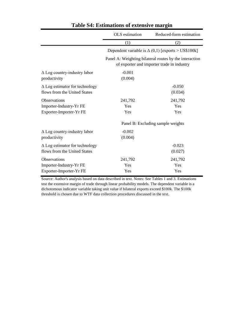
OLS estimation Reduced-form estimation

(1) (2)

Δ Log country-industry labor -0.001productivity (0.004)

Δ Log estimator for technology -0.050flows from the United States (0.034)

Observations 241,792 241,792Importer-Industry-Yr FE Yes YesExporter-Importer-Yr FE Yes Yes

Δ Log country-industry labor -0.002productivity (0.004)

Δ Log estimator for technology -0.023flows from the United States (0.027)

Observations 241,792 241,792Importer-Industry-Yr FE Yes YesExporter-Importer-Yr FE Yes Yes

Table S4: Estimations of extensive margin

Panel A: Weighting bilateral routes by the interaction of exporter and importer trade in industry

Panel B: Excluding sample weights

Source: Author's analysis based on data described in text. Notes: See Tables 1 and 3. Estimations test the extensive margin of trade through linear probability models. The dependent variable is a dichotomous indicator variable taking unit value if bilateral exports exceed $100k. The $100k threshold is chosen due to WTF data collection procedures discussed in the text.

Dependent variable is Δ (0,1) [exports > US$100k]

(1) (2) (3) (4) (5) (6)

Δ Log estimator for technology 0.589** 0.524** 0.938*** 0.886***flows from the United States, (0.272) (0.241) (0.298) (0.272)lagged five years

Δ Log estimator for technology 0.376* 0.275 0.393 0.223flows from the United States, (0.212) (0.169) (0.253) (0.256)contemporaneous

Observations 103,839 103,839 103,839 103,839 103,839 103,839Importer-Industry-Yr FE Yes Yes Yes Yes Yes YesExporter-Importer-Yr FE Yes Yes Yes Yes Yes Yes

Δ Log estimator for technology 0.267*** 0.265*** 0.648*** 0.636***flows from the United States, (0.078) (0.078) (0.112) (0.107)lagged five years

Δ Log estimator for technology 0.064 0.059 0.473*** 0.459***flows from the United States, (0.071) (0.069) (0.111) (0.105)contemporaneous

Observations 103,839 103,839 103,839 103,839 103,839 103,839Importer-Industry-Yr FE Yes Yes Yes Yes Yes YesExporter-Importer-Yr FE Yes Yes Yes Yes Yes Yes

Table S5: Lag structure of first-stage and reduced-form estimations

Panel A: Weighting bilateral routes by the interaction of exporter and importer trade in industry

Panel B: Excluding sample weights

Source: Author's analysis based on data described in text. Notes: See Table 3. The first-stage and reduced-form performance of the lagged technology flows, the preferred instrument, is contrasted with contemporaneous flows.

DV: Δ Log country-industry labor productivity DV: Δ Log bilateral exports

DV: Δ Log country-industry labor productivity DV: Δ Log bilateral exports

First-stage estimation Reduced-form estimation

Base estimation (Column 3,

Table 3)

Excluding exports

from Brazil

Excluding exports

from China

Excluding electrical

machinery

Using a 2%/98%

winsorized sample

Using ISIC 2-digit level

industry groups

Kerr (2008) sample

using Imp-ISIC2-Year fixed effects

Kerr (2008) sample

using Imp-ISIC3-Year fixed effects

Using exporter-

level clustering

(1) (2) (3) (4) (5) (6) (7) (8) (9)

Δ Log country-industry labor 1.592** 1.616** 1.372** 1.616** 1.715** 0.673* 1.109*** 1.794** 1.592***productivity (0.637) (0.644) (0.649) (0.746) (0.717) (0.393) (0.390) (0.770) (0.335)

Observations 103,839 103,010 101,221 97,326 103,839 51,483 23,345 23,345 103,839Importer-Industry-Yr FE Yes Yes Yes Yes Yes Yes Yes Yes YesExporter-Importer-Yr FE Yes Yes Yes Yes Yes Yes Yes Yes Yes

Δ Log country-industry labor 2.429*** 2.485*** 2.331*** 3.415** 2.862*** 1.578 3.448* -0.808 2.429***productivity (0.791) (0.801) (0.778) (1.735) (0.851) (1.452) (2.059) (2.094) (0.646)

Observations 103,839 103,010 101,221 97,326 103,839 51,483 23,345 23,345 103,839Importer-Industry-Yr FE Yes Yes Yes Yes Yes Yes Yes Yes YesExporter-Importer-Yr FE Yes Yes Yes Yes Yes Yes Yes Yes Yes

Table S6a: Basic robustness checks on IV specifications

Panel A: Weighting bilateral routes by the interaction of exporter and importer trade in industry

Panel B: Excluding sample weights

Source: Author's analysis based on data described in text. Notes: See Table 3.

The dependent variable is Δ log bilateral exports on the intensive margin by exporter-importer-industry

Base estimation (Column 2,

Table 3)

Excluding exports

from Brazil

Excluding exports

from China

Excluding electrical

machinery

Using a 2%/98%

winsorized sample

Using ISIC 2-digit level

industry groups

Kerr (2008) sample

using Imp-ISIC2-Year fixed effects

Kerr (2008) sample

using Imp-ISIC3-Year fixed effects

Using exporter-

level clustering

(1) (2) (3) (4) (5) (6) (7) (8) (9)

Δ Log estimator for tech 0.938*** 0.956*** 0.698*** 0.748*** 1.044*** 0.597 0.948*** 0.794** 0.938**flows from the United States (0.298) (0.299) (0.220) (0.288) (0.304) (0.387) (0.265) (0.325) (0.434)

Observations 103,839 103,010 101,221 97,326 103,839 51,483 23,345 23,345 103,839Importer-Industry-Yr FE Yes Yes Yes Yes Yes Yes Yes Yes YesExporter-Importer-Yr FE Yes Yes Yes Yes Yes Yes Yes Yes Yes

Δ Log estimator for tech 0.648*** 0.664*** 0.602*** 0.545*** 0.764*** 0.259* 0.583*** -0.079 0.648***flows from the United States (0.112) (0.112) (0.110) (0.110) (0.123) (0.141) (0.180) (0.200) (0.177)

Observations 103,839 103,010 101,221 97,326 103,839 51,483 23,345 23,345 103,839Importer-Industry-Yr FE Yes Yes Yes Yes Yes Yes Yes Yes YesExporter-Importer-Yr FE Yes Yes Yes Yes Yes Yes Yes Yes Yes

Table S6b: Reduced forms for Table S6a

The dependent variable is Δ log bilateral exports on the intensive margin by exporter-importer-industry

Panel A: Weighting bilateral routes by the interaction of exporter and importer trade in industry

Panel B: Excluding sample weights

Source: Author's analysis based on data described in text. Notes: See Table 3.

Base estimation (Column 3,

Table 3)

Using total technology trend with all ethnic groups

Weighting patents by backwards

Anglo-Saxon cites

Using industry

groupings based on mfg roles

Using first-generation immigrants

Using later-generation immigrants

Using bachelor's educated workers

Using non-bachelor's educated workers

Using 1990 ancestry

distribution for city weights

(1) (2) (3) (4) (5) (6) (7) (8) (9)

Δ Log country-industry labor 1.592** 1.513*** 2.812** 2.634* 1.581*** 1.699 2.233** 1.607** 1.888**productivity (0.637) (0.498) (1.118) (1.583) (0.420) (1.097) (1.052) (0.683) (0.815)

Observations 103,839 103,839 103,839 103,839 103,839 103,839 103,839 103,839 103,839Importer-Industry-Yr FE Yes Yes Yes Yes Yes Yes Yes Yes YesExporter-Importer-Yr FE Yes Yes Yes Yes Yes Yes Yes Yes Yes

Δ Log country-industry labor 2.429*** 3.342*** 3.085** Invalid 2.645*** 2.341** 2.727*** 2.812*** 2.650***productivity (0.791) (1.096) (1.538) first stage (0.733) (1.062) (0.988) (0.962) (0.825)

Observations 103,839 103,839 103,839 103,839 103,839 103,839 103,839 103,839 103,839Importer-Industry-Yr FE Yes Yes Yes Yes Yes Yes Yes Yes YesExporter-Importer-Yr FE Yes Yes Yes Yes Yes Yes Yes Yes Yes

Table S7a: Variations in IV design structure

The dependent variable is Δ log bilateral exports on the intensive margin by exporter-importer-industry

Panel A: Weighting bilateral routes by the interaction of exporter and importer trade in industry

Panel B: Excluding sample weights

Source: Author's analysis based on data described in text. Notes: See Table 3.

Variations in city-industry trend term Variations in city cross-sectional term

Base estimation (Column 2,

Table 3)

Using total technology trend with all ethnic groups

Weighting patents by backwards

Anglo-Saxon cites

Using industry

groupings based on mfg roles

Using first-generation immigrants

Using later-generation immigrants

Using bachelor's educated workers

Using non-bachelor's educated workers

Using 1990 ancestry

distribution for city weights

(1) (2) (3) (4) (5) (6) (7) (8) (9)

Δ Log estimator for tech 0.938*** 0.999*** 0.795*** 0.248** 1.257*** 0.570* 1.224*** 0.893*** 1.126***flows from the United States (0.298) (0.311) (0.158) (0.111) (0.387) (0.269) (0.323) (0.300) (0.314)

Observations 103,839 103,839 103,839 103,839 103,839 103,839 103,839 103,839 103,839Importer-Industry-Yr FE Yes Yes Yes Yes Yes Yes Yes Yes YesExporter-Importer-Yr FE Yes Yes Yes Yes Yes Yes Yes Yes Yes

Δ Log estimator for tech 0.648*** 0.789*** 0.374*** 0.124*** 0.875*** 0.386*** 0.637*** 0.650*** 0.766***flows from the United States (0.112) (0.107) (0.063) (0.044) (0.144) (0.102) (0.118) (0.105) (0.120)

Observations 103,839 103,839 103,839 103,839 103,839 103,839 103,839 103,839 103,839Importer-Industry-Yr FE Yes Yes Yes Yes Yes Yes Yes Yes YesExporter-Importer-Yr FE Yes Yes Yes Yes Yes Yes Yes Yes Yes

Source: Author's analysis based on data described in text. Notes: See Table 3.

Table S7b: Reduced forms for Table S7aVariations in city-industry trend term Variations in city cross-sectional term

The dependent variable is Δ log bilateral exports on the intensive margin by exporter-importer-industry

Panel A: Weighting bilateral routes by the interaction of exporter and importer trade in industry

Panel B: Excluding sample weights

Base estimation (Column 3,

Table 3)

Excluding nations with fewer than 100 data points

Excluding nations with fewer than 1000 data

points

Excluding nations with fewer than 2000 data

points

Examining long-term

OECD nations only

Excluding exporters

with <100k ethnic US members

Excluding largest foreign

patenting industry

Excluding 5 largest foreign

patenting industries

Excluding largest foreign

productivity outlier

Excluding 5 largest foreign

productivity outliers

(1) (2) (3) (4) (5) (6) (7) (8) (9) (10)

Δ Log country-industry labor 1.592** 1.590** 1.470** 1.417** 1.322 1.669** 2.023* Invalid 1.520** 2.563*productivity (0.637) (0.636) (0.568) (0.614) (0.816) (0.797) (1.098) first stage (0.586) (1.554)

Observations 103,839 103,013 89,059 71,779 74,087 78,411 97,011 73,518 100,740 82,939Importer-Industry-Yr FE Yes Yes Yes Yes Yes Yes Yes Yes Yes YesExporter-Importer-Yr FE Yes Yes Yes Yes Yes Yes Yes Yes Yes Yes

Δ Log country-industry labor 2.429*** 2.426*** 2.315*** 1.900*** 2.205** 2.251*** 3.072*** 3.257* 2.853*** 2.923***productivity (0.791) (0.787) (0.764) (0.671) (0.874) (0.875) (1.179) (1.843) (0.931) (1.081)

Observations 103,839 103,013 89,059 71,779 74,087 78,411 97,011 73,647 100,740 82,939Importer-Industry-Yr FE Yes Yes Yes Yes Yes Yes Yes Yes Yes YesExporter-Importer-Yr FE Yes Yes Yes Yes Yes Yes Yes Yes Yes Yes

Table S8a: Variations in IV sample composition

The dependent variable is Δ log bilateral exports on the intensive margin by exporter-importer-industry

Panel A: Weighting bilateral routes by the interaction of exporter and importer trade in industry

Panel B: Excluding sample weights

Source: Author's analysis based on data described in text. Notes: See Table 3.

Base estimation (Column 2,

Table 3)

Excluding nations with fewer than 100 data points

Excluding nations with fewer than 1000 data

points

Excluding nations with fewer than 2000 data

points

Examining long-term

OECD nations only

Excluding exporters

with <100k ethnic US members

Excluding largest foreign

patenting industry

Excluding 5 largest foreign

patenting industries

Excluding largest foreign

productivity outlier

Excluding 5 largest foreign

productivity outliers

(1) (2) (3) (4) (5) (6) (7) (8) (9) (10)

Δ Log estimator for tech 0.938*** 0.937*** 0.936*** 0.904*** 0.622*** 0.975*** 0.898*** 0.716*** 0.948*** 0.747***flows from the United States (0.298) (0.298) (0.308) (0.341) (0.239) (0.352) (0.175) (0.249) (0.302) (0.274)

Observations 103,839 103,013 89,059 71,779 74,087 78,411 97,011 73,518 100,740 82,939Importer-Industry-Yr FE Yes Yes Yes Yes Yes Yes Yes Yes Yes YesExporter-Importer-Yr FE Yes Yes Yes Yes Yes Yes Yes Yes Yes Yes

Δ Log estimator for tech 0.648*** 0.653*** 0.668*** 0.634*** 0.580*** 0.601*** 0.657*** 0.529*** 0.655*** 0.619***flows from the United States (0.112) (0.113) (0.120) (0.135) (0.124) (0.124) (0.115) (0.124) (0.116) (0.126)

Observations 103,839 103,013 89,059 71,779 74,087 78,411 97,011 73,647 100,740 82,939Importer-Industry-Yr FE Yes Yes Yes Yes Yes Yes Yes Yes Yes YesExporter-Importer-Yr FE Yes Yes Yes Yes Yes Yes Yes Yes Yes Yes

Table S8b: Reduced forms for Table S8a

The dependent variable is Δ log bilateral exports on the intensive margin by exporter-importer-industry

Panel A: Weighting bilateral routes by the interaction of exporter and importer trade in industry

Panel B: Excluding sample weights

Source: Author's analysis based on data described in text. Notes: See Table 3.