Work ing PaPer Ser ieSno 1527 / march 2013

heterogeneouS tranSmiSSion mechaniSm

monetary Policy andfinancial fragility

in the euro area

Matteo Ciccarelli, Angela Maddaloni and José-Luis Peydró

In 2013 all ECB publications

feature a motif taken from

the €5 banknote.

note: This Working Paper should not be reported as representing the views of the European Central Bank (ECB). The views expressed are those of the authors and do not necessarily reflect those of the ECB.

© European Central Bank, 2013

Address Kaiserstrasse 29, 60311 Frankfurt am Main, GermanyPostal address Postfach 16 03 19, 60066 Frankfurt am Main, GermanyTelephone +49 69 1344 0Internet http://www.ecb.europa.euFax +49 69 1344 6000

All rights reserved.

ISSN 1725-2806 (online)EU Catalogue No QB-AR-13-024-EN-N (online)

Any reproduction, publication and reprint in the form of a different publication, whether printed or produced electronically, in whole or in part, is permitted only with the explicit written authorisation of the ECB or the authors.

This paper can be downloaded without charge from http://www.ecb.europa.eu or from the Social Science Research Network electronic library at http://ssrn.com/abstract_id=2233313.

Information on all of the papers published in the ECB Working Paper Series can be found on the ECB’s website, http://www.ecb.europa.eu/pub/scientific/wps/date/html/index.en.html

AcknowledgementsWe are in debt with three anonymous referees for the useful comments and suggestions received. We would also like to thank the participants at the ECB seminar for stimulating discussions, and Philippine Cour-Thimann and several other colleagues at the ECB who have helped us in collecting all the relevant data. The views expressed in this paper are those of the authors and should not be attributed to the European Central Bank or the Eurosystem.

Matteo CiccarelliEuropean Central Bank; e-mail: matteo.ciccarelli@ecb.europa.eu

Angela Maddaloni (corresponding author)European Central Bank; e-mail: angela.maddaloni@ecb.europa.eu

José-Luis PeydróUniversitat Pompeu Fabra and Barcelona GSE; e-mail: jose.peydro@upf.edu

ABSTRACT The Euro area economic activity and banking sector have shown substantial fragility over the

last years with remarkable country heterogeneity. Using detailed data on lending conditions and

standards, we analyse how financial fragility has affected the transmission mechanism of the

single Euro area monetary policy during the crisis until the end of 2011. The analysis shows that

the monetary transmission mechanism has been time-varying and influenced by the financial

fragility of the sovereigns, banks, firms and households. The impact of monetary policy on

aggregate output is stronger during the financial crisis, especially in countries facing increased

sovereign financial distress. This amplification mechanism, moreover, operates mainly through

the credit channel, both the bank lending and the non-financial borrower balance-sheet channel.

Our results suggest that the bank-lending channel has been partly mitigated by the ECB non-

standard monetary policy interventions. At the same time, when looking at the transmission

through banks of different sizes, it seems that, until the end of 2011, the impact of credit

frictions of borrowers have not been significantly reduced, especially in distressed countries.

Since small banks tend to lend primarily to SME, we infer that the policies adopted until the end

of 2011 might have fall short of reducing credit availability problems stemming from

deteriorated firm net worth and risk conditions, especially for small firms in countries under

stress.

Keywords: Heterogeneity, credit channel, financial crisis, monetary policy, non-standard

measures

JEL: E44, E52, E58, G01, G21, G28

1

NON-TECHNICAL SUMMARY The financial crisis that started in 2007 has had a strong overall impact on the economy of the

euro area, but different effects across the euro area countries. While earlier on financial

integration and an appropriate functioning of macro-financial linkages had ensured that the

monetary policy of the ECB would transmit homogeneously to the whole area, since 2008 the

interconnections between market segments have largely broken, also across borders, and the

ECB has operated in a context of heterogeneity and segmentation in the money and financial

markets.

The aim of this paper is to analyse the effect of the standard monetary policy during the crisis

and to gauge whether the functioning of the transmission mechanism is smooth across the euro

area. The analysis shows how financial fragility of financial intermediaries and of borrowers

(the non-financial sector) has affected the monetary policy transmission in the euro area, in

particular through the credit channel. The study addresses several dimensions of heterogeneity,

in particular: (1) changes over time (i.e. at different moments of the crisis); (2) differences in the

impact of monetary policy in countries under financial/sovereign stress and in other euro area

countries; (3) transmission of monetary policy through all the credit channels – channels related

to the balance sheet positions of the banks (the bank lending channel) and channels related to

the worthiness of the borrowers (borrower’s balance sheet channels); and (4) differences due to

bank (and firm) size, which are key determinants of credit access.

The study is based on a Vector Autoregression (VAR) model estimated recursively over the

sample 2002Q4-2011Q3 for a panel of 12 euro area countries. The model accounts also for the

non-standard monetary policy measures implemented until the end of 2011 (in particular the full

allotment policy and the increased provision of long-term refinancing). The transmission

through the credit channel is identified using the responses of the euro area Bank Lending

Survey (BLS) at the country level. Specifically, the different channels of transmission are

identified by looking at the factors affecting the decision of banks to change lending conditions

and standards for their borrowers. Factors related to bank balance sheet capacity and

competitive pressures identify the bank lending channel, since the decisions to change these

lending conditions apply to all borrowers independently of their credit quality. The factors

linked to borrowers’ creditworthiness and net worth characterise the (borrower) balance sheet

channel. Finally the BLS information on loan demand helps to further isolate the credit demand

channel.

Based on this framework, it is possible to study the extent to which a reduced ability of banks to

provide credit to the private sector – this is how bank financial fragility is defined here – or the

2

fragility of firms and households – impaired access to credit – can amplify the impact of

monetary policy on the real economy (and on inflation).

The analysis suggests that the effect of the bank lending channel has been partly mitigated

especially in 2010-2011 by the policy actions. By providing ample liquidity through the full

allotment policy and the Longer-Term refinancing Operations (LTROs), the ECB was able to

reduce the costs arising to banks from the restrictions to private liquidity funding by effectively

substituting the interbank market and inducing a softening of lending conditions. At the same

time, when looking at the transmission through banks of different sizes, it seems that, until the

end of 2011, the impact of credit frictions of borrowers has not been significantly reduced,

especially in distressed countries. Since small banks tend to lend primarily to Small and

Medium Enterprises (SMEs), we infer that the policy framework until the end of 2011 might

have been insufficient to reduce credit availability problems stemming from deteriorated firm

net worth and risk conditions, especially for small firms in countries under stress.

The analysis therefore supports the complementary actions that have been put in place

successively, and in particular those specifically targeted at increasing credit to small firms to

reduce their external finance premia and credit rationing. In fact, the decision to enlarge the

collateral framework of the Eurosystem – in particular by accepting loans to SME as eligible

collateral – had the explicit objective of meeting the demand for liquidity from banks in order to

support lending to all type of firms.

3

1 INTRODUCTION The crisis has had a strong overall impact on the Euro area, but with substantial heterogeneity

across the various member countries. The problems in the aggregate Euro area economy and

banking sector hide a considerable degree of country heterogeneity, in terms of credit

developments, financial fragility of borrowers, lenders and sovereigns and real activity. The

single monetary policy has been the key policy implemented over all member countries to

overcome the negative effects of the banking crisis and financial fragility. Therefore, a key

question arises: what are the effects of the single Euro area monetary policy on a heterogeneous

set of economies?

Exploiting several crucial dimensions of heterogeneity, we analyse how financial fragility has

affected the transmission of the single monetary policy in the Euro area. We analyse the

heterogeneity of the monetary transmission channel considering the following key dimensions:

(1) changes over time of the transmission (before the crisis and at different moments of the

crisis); (2) differences in the impact of monetary policy shocks in countries under substantial

financial sovereign stress and in the other Euro area countries; (3) transmission of monetary

policy through the broad credit channel and its sub-channels – the bank lending and the non-

financial borrower balance sheet channels; (4) differences due to bank and firm size, key

determinant of credit access.1

The analysis is based on a flexible vector autoregression model estimated recursively and where

data on credit conditions and standards are included. Credit conditions are explicitly taken into

account using the responses by country of the Euro area Bank Lending Survey (BLS) that

provides this information with two crucial features. First, the BLS reports lending conditions for

the entire pool of applicants, including potential borrowers that are rejected. Second, it is

possible to characterize changes in lending conditions due to either a reduced capacity of banks

to provide credit to the private sector because of bank balance sheet problems, or due to the

problems in net worth, risk and collateral of non-financial borrowers (firms and households).

This information, therefore, allows the identification of the credit channel of monetary policy

and its sub-channels (Bernanke and Gertler, 1995). The model is also estimated recursively. In

this way we can assess how the monetary transmission has changed over time especially

compared with the situation prevailing at the peak of the crisis and also the impact of increased

heterogeneity in financial fragility between sovereign distressed and other countries.2

1 See Bernanke and Gertler (1995) and Bernanke (2007) for the definitions of the (broad) credit channel of monetary policy, the non-financial

borrower (firm and household) balance sheet channel, and the bank lending channel (or bank balance sheet channel). 2 See section 2 for a detailed explanation on how we define these two groups of countries. The set of (high) sovereign distressed countries are Greece,

Ireland, Italy, Portugal and Spain.

4

To analyse how financial fragility has affected the transmission mechanism, we first compare

the effect of a monetary policy shock on GDP growth and inflation before and during the

different moments of the crisis, therefore assessing whether the transmission mechanism has

changed over this time period. We do this for the aggregate Euro area but also distinguishing

between sovereign distressed countries and other countries. Second, we relate the changes in the

monetary transmission to the broad credit channel and its sub-channels, considering frictions in

borrowing for both banks and non-financial borrowers due to balance sheet constraints. These

frictions give rise to the bank lending channel and the non-financial borrower channel (see

Bernanke and Gertler, 1995, Bernanke, 2007). The testable predictions from these channels can

be mapped into BLS observables, i.e. monetary shocks affect GDP through changes in lending

conditions stemming from bank and borrower balance sheet strength. Third, we also analyze the

role of heterogeneity in bank and firm size for the transmission channel. Finally, to gain further

insights on the results, we provide evidence on the relationships between public liquidity,

private liquidity, and lending conditions, by running a dynamic panel single-equation regression

analysis.

The analysis shows that the transmission mechanism of the single monetary policy is time-

varying and influenced by the financial fragility of the sovereign, the banking sector and the

non-financial borrowers. The impact of a monetary policy shock on aggregate output is stronger

at the height of the financial crisis, even more in countries under sovereign stress. That is, a

decrease in the overnight rate implies a stronger real impact in countries with more need for

stimulus than others, precisely during the worst moments of the financial crisis – the period after

Lehman and the period after the start of the sovereign crisis.

We rationalize the previous results referring to the credit channel theory: as we are observing

the marginal effect of a monetary policy shock in economies where the financial frictions in the

credit markets have substantially increased, implying a higher external finance premium to be

paid by borrowers (firms, households and also banks), the effect of a monetary policy shock on

GDP – via the credit channel – should be higher (see Bernanke and Gertler, 1995; Kashyap and

Stein, 2000; and Bernanke 2007). We therefore analyse in detail the credit channel of monetary

policy. We indeed find that the monetary transmission via the credit channel is stronger in

sovereign stressed countries during the crisis, both through the bank lending and the non-

financial borrower balance sheet channels.3

3 The focus of our analysis is the transmission of monetary policy through the credit channels. However, as in the seminal paper by

Bernanke and Gertler (1995), we do not consider the credit channel as alternative to the traditional monetary transmission mechanism, but rather as a set of factors that amplify conventional interest rate effects. We aim at quantify this amplification mechanism.

5

However, our results suggest that the bank lending channel has been partly mitigated during the

last two years of our sample, consistently with the idea that the liquidity frictions in the banking

sector that were amplified during the peak of the financial crisis in 2008-2009 were alleviated in

2010-2011 by the non-standard policy actions of central banks. Our results suggest that by

providing ample public liquidity through the full allotment policy and the long-term refinancing

operations (LTROs), the Eurosystem was able to reduce the costs arising to banks from the

restrictions to private liquidity funding by effectively partly substituting the interbank market

and, in turn, inducing a subsequent softening of lending conditions.

While we argue that the bank balance sheet problems relative to liquidity might have been

mitigated by the ECB interventions, at the same time, when looking at the transmission through

banks of different sizes, it seems that, until the end of 2011, the impact of credit frictions of

borrowers have not been significantly reduced, especially in distressed countries. Since small

banks tend to lend primarily to SME, we infer that the policy framework until the end of 2011

might have been insufficient to reduce credit availability problems stemming from deteriorated

firm net worth and risk conditions, especially for small firms in countries under stress.

This conclusion therefore supports the complementary actions undertaken in successive periods,

in particular those specifically targeted at increasing credit to small firms in order to reduce their

external finance premia and credit rationing.

This paper makes three main contributions with respect to the related literature . First, we

analyze heterogeneity in the transmission mechanism of monetary policy. We measure the

impact of a single monetary policy in a set of heterogeneous countries and find important effects

on GDP of monetary policy. However, these effects are heterogeneous across countries, time

periods and monetary channels, and with important limitations in scope (limited impact on

credit conditions for small firms due to the firm channel) that suggest the need for other

complementary policies. By doing this, we depart from the analysis reported in Ciccarelli,

Maddaloni and Peydró (2011), where we did neither consider heterogeneity issues nor time

variation. Second, the identification of the credit channel of monetary policy has advanced by

analyzing heterogeneous effects across banks (Kashyap and Stein 2000 and Jiménez et al.

2012). We complement this literature by analyzing the heterogeneous effects across normal and

crisis times, stressed and non-stressed countries, and the credit channel (and its bank and non-

financial borrower sub-channels). In this framework in particular, our analysis differs compared

with Lenza, Pill and Reichlin (2011) – who do not explicitly consider (credit) channels of

transmission of monetary policy – and with Darracq and De Santis (2013) – who focus instead

on the macroeconomic impact of credit supply shocks. Finally, we give some evidence on the

effects of non-standard monetary policy tools during the crisis, by analyzing the impact of

6

aggregate Euro area long-term public liquidity on GDP through the overnight interbank rate,

controlling for the heterogeneous (country-based) long-term public liquidity and other key

variables, and also by providing dynamic correlations between the Eurosystem liquidity,

interbank liquidity and change in lending standards.

The rest of the paper is structured as follows: In section 2 we motivate our work with a reasoned

narrative of the crisis. In section 3 we present the empirical analysis discussing the data, the

identification strategy and the estimation methodology. In section 4 we discuss the main results

and their policy implications. Section 5 concludes.

7

2 MOTIVATION AND AIM: A REASONED NARRATIVE OF THE CRISIS

In this section we set the scene for the subsequent analysis and briefly describe the events that

occurred during the crisis and the reaction of the central banks, in particular in the Euro area.

We connect the main elements that are the focus of the paper, i.e. the financial fragility of

sovereigns, their banks and borrowers, monetary policy and its transmission, and the lending

conditions and standards (using the BLS data).

The unfolding of the financial crisis resulted in a significant tightening of financing conditions

for both corporates and banks starting already in August 2007. For illustration, in Figure 1 Panel

A, we plot a financing condition indicator calculated using data from different financial

markets, which shows that financing conditions became particularly tight in 2007, when the

problems in the subprime markets in the US came to surface. However, conditions worsened

dramatically later on, to reach a minimum after the bankruptcy of Lehman Brothers.

Central banks reacted swiftly by lowering policy rates and, in the Euro area, by changing the

terms for the liquidity provision to the banking sector. Liquidity provision moved to a fixed rate

full allotment policy – banks could come at the Eurosystem liquidity operations and ask for

unlimited amount of liquidity at the policy rate. Financing conditions remained nevertheless

tight, since the liquidity provided by the operations could fill only very short-term liquidity

needs. The Eurosystem stepped up the pace of its longer-term operations (liquidity provided for

three-months and six-months) and announced three one-year long-term operations that were

conducted in June, October and December 2009. These operations, in conjunction with a lower

level of policy rates, resulted in a more accommodative policy stance for the Euro area. Indeed

the indicator of Panel A suggests looser financing conditions in 2010 and 2011 for the whole

Euro area. The ECB implemented also other non-standard measures over the last few years,

although the scale of these measures was somewhat more contained.4 We do not explicitly

control for all these aggregate measures as they have important effects on the Euro area

overnight interest rates that we exploit in our econometric analysis (see next section) and,

moreover, most of their impact is indirectly embedded in the heterogeneous access to liquidity

provisions by the different countries, a variable that we explicitly include in our model, and

would result in a relaxation of lending conditions.

4 In fact, the ECB implemented FX swap agreements, enlarged in several steps the set of eligible collateral to use in the repo refinancing operations,

bought covered bonds and governments bonds (the Securities Markets Programme, SMP) of countries under stress. All these measures aimed at increasing bank balance sheet capacity by expanding the set of assets that could be brought to the ECB to obtain liquidity (collateral eligibility), supporting the value of these assets (covered bond purchase and SMP) and facilitating access to foreign currency liquidity.

8

The indicator shown in Panel A gives a very aggregate picture of financing conditions,

measuring the ability of both corporates and banks to access funding. However, the tight

financing conditions were particularly negative for the banking sector.

In Panel B, we plot the spread between the Euribor and the Eurepo interbank rates for the one

year and one week maturities. Until the summer of 2007 these spreads were very low, in the

range of few basis points, and slightly higher for the long maturities. With the unfolding of the

crisis the spreads increased dramatically, due to both counterparty and liquidity risk. Financing

conditions for the banking sector remained very tight, with the interbank market having lost its

funding function; this situation in turn exacerbated problems in the balance sheet positions of

the banks. While the liquidity provision of the Eurosystem likely helped in decreasing these

rates after the Lehman episode – especially for shorter maturities – the spreads remained

historically high, in particular for longer maturities. The start of the sovereign crisis in the Euro

area again triggered increases in these spreads, although their levels remained substantially

lower than in the Lehman period.

While differences in the perceived country risks in the Euro area became particularly evident in

2010 and 2011 with the unfolding of the sovereign crisis, already in 2008 the credit risk of the

single Euro area countries started to be effectively priced, as evident for example by the

divergent patterns in the credit default swaps (CDS) of the sovereign 10 year bonds (see Panel

C). Starting from this observation, we divide the countries in two groups, the countries under

sovereign stress (Greece, Ireland, Italy, Portugal and Spain) and the other countries (Austria,

Belgium, Finland, France, Germany, Luxembourg, Netherlands),5 and use this working

definition throughout the paper. Facing difficulties in raising private funds, banks in the stressed

countries turned more to the liquidity provided by the Eurosystem, especially long-term. Panel

D plots the long-term liquidity (maturity greater or equal than 3-month and up to 1 year) taken

by banks of the countries under stress and by banks of the core countries over the last few years

as a percentage of the banks’ assets in each country – the liquidity taken at the Longer-Term

Refinancing Operations (LTROs). Starting in 2010 this difference increased significantly,

generating an increasing asymmetry, demand-driven, in the transmission of monetary policy

across countries.

Standard and non-standard measures of monetary policy affect the willingness and ability of

banks to grant credit to the corporate and household sector. Figure 2, Panel A, shows that

lending conditions and standards, measured by the BLS, diverged significantly since the start of

the financial crisis in the two groups of countries, with more tightening of lending conditions

5 We restrict the analysis in the paper to the 12 countries in the Euro area when the BLS was implemented (2002:Q4) and for which the entire time

series is available.

9

and standards in the countries under stress (see Section 3.1. and Table A.1 in the Appendix for a

detailed description of the BLS data). At the same time, demand for business loans started to

decline in all countries already at the beginning of the crisis. However, only in the very last

period of our sample the demand for loans in the two groups of countries significantly departed

from each other (see Figure 2, Panel B).

The analysis that follows aims at investigating monetary policy transmission in the Euro area

during the crisis (as compared to normal times), focusing on the issues raised above and notably

differentiating the results between stressed and other countries. First, we look at the impact of

the monetary policy transmission channel, focusing on different moments of the crisis and some

specific dates linked also to the refinancing operations of the Eurosystem. Next, based on the

results of the first step of the analysis, we focus on the broad credit channel and distinguish

between the bank and the non-financial borrower balance sheet channel. Finally, we assess the

credit channels exploiting heterogeneity across bank (firm) size. In the last part of the paper, we

run a series of dynamic panel regressions to investigate the relationships between public

liquidity, private liquidity, and lending conditions to gain further insights on the results.

10

3 THE EMPIRICAL ANALYSIS The analysis is based on a multivariate dynamic panel data model of the type developed by

Ciccarelli, Maddaloni, Peydró (2011), CMP henceforth –, i.e. a panel VAR model which

includes macroeconomic and financial time series by country.

The model has the following specification:

Ω (1)

where is a vector of endogenous variables containing output, prices, monetary policy rate,

interbank lending volumes, long-term ECB lending to the banking sector, long term-interest

rates, lending conditions and loan demand from the BLS (see section 3.1 for details). All

variables are at country level, except for the monetary policy rate which is common across all

countries. is a vector of fixed effects; is a matrix polynomial of slopes in the lag

operator ; Ω is the contemporaneous impact matrix of the mutually uncorrelated structural

shocks that have zero mean and identity variance-covariance matrix.

In what follows, we discuss and motivate the data used in the VAR analysis, the identification

schemes and the estimation issues.

3.1 DATA

The data used in the analysis have quarterly frequency. This is dictated by the frequency of

macroeconomic data series and the BLS. Output and prices – which account for the general

macroeconomic conditions – are proxied by the four-quarter GDP growth rates and inflation

(GDP deflator).6

A crucial issue concerns the variable used to identify the single Euro area monetary policy

shocks. We use the overnight (EONIA) rate. The Governing Council of the ECB sets three key

policy rates: the rates for the deposit facility, the main refinancing operations and the marginal

lending facility. These rates constitute the corridor in which the overnight rate fluctuates. Until

the end of 2008, EONIA has been practically indistinguishable from the rate of the main

refinancing operations (MRO). With the unfolding of the crisis and the ECB decision to provide

liquidity to the banking sector in unlimited amount, the EONIA rate dropped below the MRO

rate, indicating that the impact of these non-standard monetary policy measures, therefore the

aggregate, systematic and unconventional part of the recent policy is broadly included in the

EONIA rate (see Trichet 2009; ECB 2009; Lenza et al. 2010 and Soares and Rodriguez 2011).

6 In the appendix all the data sources are reported in detail, see Table A.1 and A.2.

11

As there is substantial country heterogeneity regarding financial conditions and the recourse to

the LTROs as shown in Figure 1, we include some additional controls in the VAR. These

controls account for the heterogeneity of the non-standard policy actions of the central bank

introduced in the last few years and of the financial conditions and, therefore, induce a correct

identification of the common monetary policy shock. For all these reasons we include in the

VAR three additional endogenous variables: (i) The volumes of transactions in the interbank

market, which proxy for bank funding conditions;7 (ii) The longer-term (3 months up to 1 year)

liquidity provided by the Eurosystem to the banking sector in each country as a fraction of total

bank assets, which broadly account for heterogeneity of the non-standard measures taken by the

ECB during the financial crisis to support financing conditions and credit flows; and (iii) the

rates on the long-term sovereign bonds which also serve as a proxy for country risks.

The inclusion of variables that capture the financial and banking sector deserves a broader

discussion given the importance they have acquired during the crisis. In fact, any analysis of the

transmission mechanism that extend over the last four years should account for the prominence

of the credit channel in the Euro area and for the impact on the provision of bank loans to

correctly distinguish monetary policy from financial shocks (CMP 2011).

In particular, a key element is the identification of possible restrictions to credit provision

(credit rationing and external finance premia) accounting for the financial fragility of both banks

and non-financial borrowers (firms and households). Our VAR model accounts for this, by

using bank loan demand and lending conditions and standards as measured by the responses of

the Bank Lending Survey (BLS). The national central banks of the Eurosystem request a

representative sample of banks in each country to provide quarterly information on the lending

standards that banks apply to borrowers and on the loan demand that banks receive. The

information concerns changes in loan conditions and demand recorded over the previous three

months, and expectations of the same figures over the following quarter. The survey focuses on

two borrowing sectors, firms and households. Household loans are further disentangled in loans

for house purchase and for consumer credit.8

The BLS represents an invaluable source of information on bank credit conditions in the Euro

area for several reasons. First, the questions refer to lending standards applied to all potential

borrowers and therefore this information does not suffer the selection bias of the measures based

on loans effectively granted (almost all measures based on hard data).9 Moreover, the BLS asks

whether, how and, notably, why lending conditions have changed. First, banks are asked

7 The volumes transacted in the interbank market are proxied by the actual transactions of the panel of banks included in the EONIA panel, as provided

by the European Banking Federation (EBF). 8 For a detailed description of the BLS see Berg et al. (2005) – that describes in detail the setup of the survey. Maddaloni and Peydró (2011) and CMP

(2011) also use the data from the BLS. 9 The only exception, in the monetary policy literature, is Jiménez et al. (2012), but they have loan applications only for one country, Spain.

12

whether they have changed lending standards over the previous quarter. Next, the BLS reports

how banks have changed terms and conditions for the loans, whether via changes in loan spread,

size, collateral requirements, maturity or covenants. Finally, the survey asks why banks have

modified their lending conditions. In particular, what has been the impact on the decision to

change lending conditions of changes in bank balance-sheet capacity (and competitive

pressures), and also in non-financial borrowers’ net worth and risk.

The focus of our analysis is the transmission of monetary policy through the credit channels.

However, as in the seminal paper by Bernanke and Gertler (1995), we do not consider the credit

channel as alternative to the traditional monetary transmission mechanism, but rather as a set

of factors that amplify conventional interest rate effects. We aim at quantify this amplification

mechanism.

The use of the BLS is crucial, as the information contained therein allows us to assess the

transmission of monetary policy through the broad credit channel. In particular, we use the

answers related to the factors affecting the decision to change lending conditions and standards

as a way to distinguish the credit (sub-)channels of transmission of monetary policy. Factors

related to bank balance sheet capacity and competitive pressures identify the bank lending

channel, since the decisions to change these lending conditions apply to all borrowers

independently of their credit quality. The factors linked to borrowers’ creditworthiness and net

worth characterise the non-financial borrower balance sheet channel. Finally the BLS

information on loan demand helps to further isolate the credit demand channel.10

The BLS provide only qualitative answers, therefore we need to construct an indicator that can

be used in the empirical analysis. The questions asked in the BLS allow for five possible replies.

The answers range from “eased considerably” to “tightened considerably” for the questions

related to changes in lending standards, and from “decreased considerably” to “increased

considerably” for the questions related to the demand for loans. We follow Lown and Morgan

(2006) and quantify the different answers by using net percentages. The answers related to the

changes in lending conditions and standards that banks apply to borrowers define the broad

credit channel variable. The measure of the broad credit channel variable is the difference

between the percentage of banks reporting a tightening of lending standards and the percentage

of banks reporting a softening of standards in each country and for each quarter. We measure

credit demand by the net percentage of banks reporting an increase in the demand for loans

received from firms and households relative to those reporting a decrease.

10 This identification strategy is implemented also in CMP (2011).

13

Moreover, we use the factors affecting banks' decisions to change lending standards to define

the (i) bank lending channel variable (factors related to bank balance sheet strength and

competition pressures) and the (non-financial) borrower's balance sheet channel variable

(factors related to the quality of loan applicants such as outlook, net worth and risk of

borrowers). The net percentage of banks that have changed standards due to factors linked to

bank balance sheet capacity and competition defines the bank lending channel variable. The net

percentage of banks that have changed standards due to factors linked to firm (household)

balance-sheet strength defines the (non-financial) borrower's balance sheet channel variables.

In all cases a positive value implies a net tightening of lending standards and, therefore, a

restriction of the terms and conditions for loans. Bank lending channel variables and borrower's

balance sheet variables are available for all type of loans. Banks are broadly classified as large

and small banks, depending on their size.

The first BLS was run in 2002:Q4 and the same set of questions has been asked consistently

through time.11 The original sample included 12 Euro area countries: Austria, Belgium, France,

Finland, Germany, Greece, Ireland, Italy, Luxembourg, the Netherlands, Portugal and Spain.

For time consistency, we restrict the analysis to this sample of countries although other Euro

area countries were added over time. The samples of banks are country specific but they are

representative of the banking sector in each country. We generally use data aggregated at

country level, but we also use information at the bank level when differentiating between large

and small banks in each country.

3.2 IDENTIFICATION

The vector in Eq. (1) contains 15 variables for each country: 6 macro and financial variables

and 9 credit variables from the BLS. The macro and financial variables are GDP growth,

inflation, EONIA rate (four-quarter change), interbank lending volumes, long-term ECB lending

(scaled by total bank assets) and long term-interest rates (four-quarter change). The nine BLS

variables are the credit demand, the bank-lending and the borrower’s balance sheet variables for

the three categories of loans (business, mortgages, consumer credit).12

The focus of this paper is on how the transmission mechanism of a (standard) monetary policy

shock might have changed in recent periods because of financial fragility in some country.

Therefore, we concentrate on the heterogeneous transmission of a standard policy shock

11 Ad hoc questions were added to address specific issues, but these were only included in addition to the standard set of questions. 12 See Table A.1 in the appendix for a summary of the variable definitions.

14

through the credit sector across countries, while we do not identify the effect of possible shocks

to the credit sector (as e.g. in Peersman 2011).

VAR models with macro and financial variables have become standard tools to identify the

effect of monetary policy shocks on the economy. In the benchmark specification, following

previous literature (e.g. Bernanke and Gertler, 1995; Christiano et al, 1996 and 2000), the

monetary policy shock is identified using (i) the overnight rate (EONIA) as the monetary policy

instrument and (ii) a triangular orthogonalization (Choleski decomposition) with a specific

ordering of variables.

The key assumption is that policy makers observe current output, prices and the results of the

bank lending surveys when deciding the policy rate. Consequently these variables do not change

contemporaneously in response to a policy shock, and the policy rate is ordered after the macro

and the BLS variables. This ordering partly differs from what typically assumed in the literature,

(as e.g. in Christiano et al. 1999), where the credit variables – typically loan volumes – are

assumed to respond to the monetary policy rate within the quarter. Our choice is motivated by

the fact that Euro area policy makers take interest rate decisions based on a strategy that

explicitly accounts for developments in the credit markets. For instance, as part of the monetary

analysis assessment (the so-called Second Pillar of the monetary policy strategy), the ECB

policy makers monitor closely the developments of the BLS.

Regarding credit variables, we assume that loan demand and lending standards referring to

different borrowers are included in the VAR following an ordering that broadly reflects the

importance of the different loan markets in the Euro area, i.e. business loans come first, then

mortgage loans and finally consumer loans, with demand being ordered before supply variables

for each loan market.

Finally, the long-term rates and the quantity variables (interbank volumes and central bank long-

term liquidity) are ordered after the policy rate. A shock in long-term rates (for instance related

to country risks), although not affecting contemporaneously the policy rate, may influence the

demand of liquidity by banks, both on the private (interbank) market and from the ECB. At the

same time, if liquidity on the interbank market dries up and banks’ access to market-based

funding erodes, this will have an impact on the recourse to long-term central bank liquidity

within the same quarter - long-term lending by the central bank is assumed to be a “last resort”

in the money market.

Summarising, our identification scheme in the VAR amounts to apply a Choleski decomposition

to the matrixΩ , with the 15 variables of the vector entering with the following ordering:

GDP growth, inflation, credit demand for the three categories of loans, bank-lending and

15

borrower’s balance sheet variables for the three categories of loans, EONIA rate (common

across countries), long term-interest rates, interbank lending volumes, and long-term ECB

lending.

Before presenting the results of the estimation based on this identification scheme, we discuss

two remarks and run some robustness analysis.

First, our objective is to check the transmission mechanism of a “standard” monetary policy

shock. While there is some broad consensus on the triangular identification of the monetary

policy shock in a three variable VAR model, the introduction of credit variables before the

policy rate in a model estimated on quarterly data needs to be verified. Therefore, we conduct

several robustness checks using different orderings of the variables in , in particular to test the

assumptions that the credit variables do not respond to monetary policy within the quarter. The

results are robust to the different specifications and the correlation matrices of the reduced-form

residuals indicate that correlations across innovations (in particular between the policy rate and

the credit variables) are small, implying that the impulse response analysis is broadly invariant

to a reordering of the variables. The correlation matrices are reported in the Appendix (see

Table A.3).

Second, regardless of the variable ordering, we perform some robustness checks with an

identification scheme based on sign restrictions.13 The signs are restricted only on the

contemporaneous impact. As we are interested mainly in the effect of the policy shock on GDP

growth, we leave the response of this variable unrestricted, and assume a negative response of

inflation to a monetary policy shock and an increase in the EONIA rate. The increase in EONIA

is assumed to influence in the same direction also the long-term interest rates and to be passed

on to the credit market with a decrease in the volume of credit demanded for all categories of

loans. At the same time, we leave unrestricted the reaction of the lending standards applied by

banks (both the bank lending and the borrower’s balance sheet variables) for all loan categories.

Finally, an increase in the EONIA rate is assumed to have a negative impact on the lending

volumes in the interbank market, while we leave unrestricted the sign of the recourse to long-

term central bank liquidity. This robustness exercise – which shows that impulse responses

obtained with the two alternative identification schemes are statistically similar – is also

reported in the Appendix (see Figure A.1).

13 We follow the sign restriction approach described in Rubio-Ramirez et al. (2010).

16

3.3 ESTIMATION

The reduced-form of the VAR in Eq. (1) is estimated over the sample 2002:Q4-2011:Q3 for the

panel of the 12 countries comprising the Euro area in 2002. The analysis is based on country

data for a two-fold purpose: (i) we exploit cross-country and heterogeneous information to

overcome an otherwise short-time span; and (ii) we structure our analysis around possible

differences across countries – in particular among countries that have been subject to different

degree of financial distress as defined in section 2.

For the estimation we allow the slopes and the contemporaneous impact matrix to be different

for the two sets of countries that we consider (i.e. countries under sovereign stress and other

countries) but we restrict them to be common within each set of countries. This implies that

equation (1) changes as follows:

, , , Ω , (1a)

where =1 or 2 identifies the two groups of countries. For each group , we estimate the model

with a country fixed-effect. We demean all variables and estimate Eq. (1a) without the constant

for each group. Over a short time span, this framework is helpful in pooling diverse information

from all countries, while controlling for the required level of heterogeneity. Cross-country

correlations are assumed to be zero both between and within groups, therefore the specification

in Eq. (1a) is not a multi-country model of the type introduced for example by Canova and

Ciccarelli (2009), given the limitation of the time span – which limits our degrees of freedom –

and the scope of the analysis – which focuses on the impact of a common shock more than on

spillovers across countries.

The model is estimated recursively and the first estimation is run over the sample 2002:Q4-

2007:Q3. In the subsequent estimations we then add one quarter at a time so that the second

estimation covers the sample 2002:Q4-2007:Q4, and so on, until the last quarter (2011:Q3) is

included. This estimation strategy allows investigating the time-varying characteristics of the

transmission of monetary policy and of the relationships among variables. It enables to identify

the marginal effects of additional quarters of data, and, therefore, to assess the evolution of the

relationships when moving from “normal” to (different) “crisis” times. An optimal lag length

equal to 1 is chosen with the Schwarz Bayesian Criterion.

We have tested the null hypothesis of parameter homogeneity across the two groups of countries

against the alternative assumed by our specification in Eq. (1a). To perform the test, we use the

general likelihood ratio

17

∙ |Σ | ∑ Σ (2)

where is the total number of observations, and are the observations in each

group of countries, Σ is the estimate of the pooled variance covariance matrix of the reduced-

form obtained estimating the model under the null of homogeneity, and Σ is the estimated

variance-covariance matrix for each group . Under the null hypothesis of homogeneity, this

statistics has an asymptotic distribution with degrees of freedom equal to the number of

restrictions imposed under the null.14 The null hypothesis is rejected with a very high degree of

confidence, supporting a heterogeneous structure across the two groups of countries.

The main results are presented and discussed by means of impulse response functions and

counterfactual experiments. With impulse response functions we analyse the responses of the

macroeconomic variables (mainly GDP growth) to a shock (increase) in the common overnight

rate and check whether these responses have changed over time and whether they are different

for the two sets of countries. Uncertainty around parameters and impulse response functions are

computed with standard Bayesian Monte Carlo methods assuming normality of the error terms

and a diffuse prior on the parameters for both sets of countries (see e.g. Kadiyala and Karlsson,

1997).15

We use counterfactual experiments to assess the impairment of the transmission mechanism due

to frictions in the credit markets amplified by the financial crisis, particularly in certain

countries. In the estimation, we construct the counterfactuals as hypothetical impulse responses

which feature only the “direct” impact of an interest rate movement on the macroeconomic

variables and neutralize the indirect effect through the BLS credit variables (channels). This is

done by constructing a hypothetical sequence of shocks to the BLS credit variables such that the

impulse response of these variables to an interest rate shock is equal to zero at all horizons.16

In principle, to zero out the responses of the credit channels and neutralise the effect of the

monetary policy shock in our triangular identification scheme, several sequences of variable

residuals could be used. However, since the BLS variables correctly identify the credit channel

variables, to neutralize the effect of the bank-lending channel, the borrower’s balance sheet

channel and the demand channel we use only the residuals of these variables for all loan

categories.

14 The restrictions are given by the number of VAR coefficients (this amounts to 152 = 225) plus the number of free parameters of the variance

covariance matrix (15x16/2 = 120). We have run the test recursively and found that on average over the recursion sample the value of the statistics is 820.

15 Note that the specification is estimated on panels which, for the full sample, contain about 180 observations for the group of countries under stress and 250 for the others. Therefore, the posterior distributions are precise and depend very little on the prior information.

16 For the same counterfactual analysis applied to a different context, see Bachmann and Sims (2012). The algebra to derive the hypothetical responses in our model is basically the same as in theirs. The approach is obviously not immune to the Lucas’ critique. However, in our context, the richness of the BLS – which allows to map the credit channel into concrete observables – and the recursive estimation – which makes the parameter structure change recursively each quarter – should make results trustworthy and less subject to the critique.

18

The comparison of these hypothetical responses with the actual responses estimated in the full

model provides a statistical measure of the importance of the credit channel and sub-channels in

the transmission of the monetary policy shock. According to the credit channel theory of

monetary policy transmission, informational and contractual frictions in credit markets worsen

during tight-money and worse-economic and financial periods. The resulting increase in the

external finance premium – the difference in cost between internal and external funding –

amplifies the effect of monetary policy on the real economy (Bernanke and Gertler, 1995). The

counterfactual analyses help us to assess this amplification and, consequently, to evaluate how

active or subject to financial frictions the channel has been over the recent period.

19

4 RESULTS Using the specifications described above, we analyse the transmission mechanism of monetary

policy in the recent years for countries under sovereign stress and for the other Euro area

countries. First, we present the responses of GDP growth and inflation to a standard monetary

policy shock; then we quantify the possible enhancement effects due to the credit channel;

finally, we check to what extent the economic and statistical significance of these results

depends on the size of the banks and firms. Finally, through a dynamic panel regression analysis

we assess the heterogeneous effects of non-standard monetary policy measures on lending

conditions.

4.1 THE EFFECTS OF MONETARY POLICY SHOCKS OVER TIME

Has the impact of a monetary policy shock changed since the beginning of the financial crisis?

Figure 3 reports three-dimensional charts with the dynamic responses of GDP growth and

inflation to a 25 basis point increase in the overnight rate from 2002:Q4 to 2011:Q3.17 The

responses are based on recursive estimations of the model. Therefore, results at each quarter

show the response of the variables of interest based on information until that quarter, with the

first estimation sample being 2002:Q4-2007:Q3, the second one 2002:Q4-2007:Q4 and the last

one 2002:Q4-2011:Q3. Among other things, this allows us to evaluate the marginal effects of

the additional information contained in the subsequent quarters after the first sample and,

therefore, analyse the different moments of the crisis.

Panel A shows the results for all the Euro area countries of our sample and its charts report

significant variation over time of the responses of GDP growth and to a much lesser extent of

inflation to the monetary policy (Euro area overnight interest rate) shock. Three distinct phases

are shown for both groups of countries. The first phase, where impulse responses are estimated

using information before the bankruptcy of Lehman Brothers, is characterized by muted and

slow responses, with e.g. an average peak impact on GDP growth of -0.1 occurring after 10

quarters. In the second phase, estimated until the fourth quarter of 2009, both the size and the

timing of the transmission have changed, with peak impacts during the height of the financial

crisis being not only substantially stronger (with values of about -0.4 per cent in 2009 for GDP

growth) but also faster by the end of it (with peaks realising after 6-8 quarters in 2009 for GDP

growth). In the most recent phase, where impulse responses are estimated using the entire

17 As the standard deviation of overnight rates varies during the crisis, we show the results with the same change in basis points for all the time

periods. The size of the response is measured on the Z-axis, the steps (quarters) of the responses are on the X-axis and the dates until which the model has been estimated are reported on the Y-axis. Note that as the VAR is linear, responses are symmetric if we consider an expansionary shock.

20

sample, responses take somewhat intermediate levels between the pre-crisis and the peak crisis

period, with peak levels of -0.25 occurring after 6-7 quarters.

If we examine the same responses for the two groups of countries based on the sovereign

financial stress, clear differences emerge (Panels B and C). The impact of a change in the

monetary rate has become significantly larger with the crisis in particular for countries under

stress (Panel B), where the peak impact on GDP growth has reached -0.5 percentage points in

2009 from about -0.2 when including data only until mid-2008. More importantly, this marked

effect has persisted and even amplified during the last part of the sample, reflecting the more

difficult economic situation that these countries have been facing since the start of the sovereign

crisis in May 2010.18

In other countries (Panel C), with substantially less sovereign stress, the three phases are

qualitatively similar to those of Panel A. Moreover, the chart shows a lower (and faster) impact

compared to the impulse responses of Panel B. These findings hold for both GDP growth and

inflation, where the typical price-puzzle is also milder at the end of the sample.19

In sum, results suggest that on average the effect of a (single) monetary policy shock on GDP

growth has been time-varying during the years of the crisis and became stronger and faster in

2008-2009. Differently, not much variation is shown for impacts on inflation. Moreover, the

impact has been substantially stronger for the sovereign stressed countries, in particular after

May 2010.

How to interpret these results? The impulse responses show that a decrease in the common

interest rate would have implied a somewhat desirable heterogeneous reaction across countries,

with a stronger real impact in countries that have been in more need for stimulus than others,

precisely during the worst moments of the financial crisis – i.e., the period after Lehman and the

period after the start of the sovereign crisis. It is important to note that we are observing a

marginal effect of a monetary policy shock in economies where the financial frictions in the

credit markets have substantially increased, implying higher external finance premia to be paid

by borrowers, being firms, households but also banks (see Figure 1 and 2 for credit conditions

during the crisis in the Euro area and the significant heterogeneity between the two sets of

countries). In this environment, the effect of a standard shock to the overnight interest rate

transmitted through the credit channel of monetary transmission should be higher (see Bernanke

and Gertler 1995; Kashyap and Stein 2000; and Bernanke 2007). The next section qualifies

18 The variability of the responses may also be partly due to the impact of different policies that were implemented during the period at different points

in time (see Section 2). 19 Countries under stress show a much less pronounced price puzzle than other countries. As suggested by a referee, this could be evidence of a more

active cost-channel in non-stressed economies, whose evidence is nevertheless difficult to prove in our framework. In alternative VAR specifications, we have used the one-year-ahead consensus forecast for country inflation to check if this price-puzzle may simply reflect mis-specifications due to the omission of a measure of inflation expectations, but we don’t find different impacts of a monetary policy shock, neither on inflation, nor on GDP growth.

21

these findings on GDP in light of the credit channel of monetary policy theory by quantifying

the (broad) credit channel and its sub-channels – the bank lending and the non-financial

borrower (firm and household) balance-sheet channels.

4.2 THE BROAD CREDIT, BANK AND NON-FINANCIAL BORROWER BALANCE SHEET

CHANNELS

In the rest of the paper, given the previous findings, we focus only on the impact of monetary

policy shocks on GDP growth. In this subsection, we explore the role of bank credit in the

transmission of a monetary policy shock by means of appropriately designed counterfactual

experiments.20 As described above, we quantify the credit channel by reporting the

amplification effect of a monetary policy (interest rate) shock due to changes in credit

conditions and terms, both through the bank and non-financial borrower balance sheet channels.

In so doing, we aim at linking the effects of monetary policy to the financial fragility of

borrowers and lenders via the credit channel of monetary transmission.

The results of the counterfactual analysis are reported in Figure 4 and 5, where we compare the

dynamics of the responses of GDP growth to a 25 basis point increase in the monetary policy

rate with the median counterfactual responses of the same variables obtained when closing

down the credit channel (solid red line). The 68% confidence interval (in blue) and the median

(black line) represent the response in a system where all the channels (variables) are active. The

red lines instead are the median responses estimated in a system where the different credit

channels or the credit demand channels have been closed down, i.e. these channels do not react

to a monetary policy impulse.

Note that a significant difference between the two lines implies that monetary policy shocks are

partly transmitted through that particular channel. To the extent that the different credit channels

are only important when significant financial frictions exist in credit markets (see e.g. Bernanke

and Gertler 1995), we can interpret the difference between the two lines as a measure of the

existence and importance of these credit frictions.

Unlike in Figure 3, for easiness of illustration, we report results here only for the two groups of

countries and only at various quarters selected as follows: the first date (2007:Q4) marks the

beginning of the financial crisis; the second date (2008:Q4) is the quarter following the Lehman

Brothers’ bankruptcy and the introduction of the fixed rate full allotment policy; the third date

(2009:Q4) is the quarter following the end of the Great recession and the implementation of

20 In the Euro area (as compared for example to the U.S.), banks are the main providers of funds to the private sector (Allen et al., 2004).

22

three one-year refinancing operations conducted by the ECB; the fourth date (2010:Q3) refers to

the quarter following the start of the sovereign crisis in the Euro area; and finally we stop the

estimation at 2011:Q3 before the introduction of the very long-term refinancing operations

(three-year maturity, VLTROs).21

Figure 4 shows that the impact of a monetary policy shock on GDP depends significantly on

changes in the transmission of the shock through both the broad credit channel proxied by the

BLS variable “changes in total lending conditions and standards” (left-hand column) and the

credit demand channel proxied by the BLS variable “changes in loan demand” (right-hand

column). This is evident in particular for countries under sovereign stress (Figure 4 Panel A),

where the effect of these channels on GDP growth are economically and statistically significant

as of 2008 and for the entire period. Conversely, for the set of other countries (Panel B), results

are marginally significant in 2008 (and 2009 for the demand channel) and clearly not significant

in 2011.

All in all, the impulse responses suggest that the impact of a monetary policy shock on GDP

growth is amplified by changes in the credit conditions and standards – the broad credit channel

is active. In other words, the amplification reflects the underlying problems in credit markets as

implied by the credit channel theory. The amplification is stronger in the countries under stress

and is significant throughout the crisis period.

To gain further insights on the mechanisms at work, we disentangle in Figure 5 the broad credit

channel distinguishing the transmission of a monetary policy shock through the bank-lending

channel from the non-financial borrower (firm and household) balance-sheet channel (see

Bernanke and Gertler, 1995; Kashyap and Stein, 2000; and Bernanke 2007). We use the BLS-

based bank lending channel variable (factors related to bank balance sheet capacity and

competition pressures) to analyse the bank lending channel and the BLS-based borrower's

balance sheet channel variable (factors related to the quality of loan applicants such as outlook,

net worth and risk of borrowers) to analyse the non-financial borrower balance sheet channel

(see section 3.1 and Table A.1 in the Appendix).

Panel A shows that the bank lending channel of monetary policy has been important only in

2008 and 2009 for stressed countries, but not statistically significant in 2010 and 2011.

However, the non-financial borrower (firm and household) channel of monetary policy has been

economically and statistically significant throughout the whole period after the Lehman

bankruptcy. Instead, for the other countries, Panel B shows that the non-financial borrower 21 The analysis in the paper includes data until 2011:Q3. Therefore, we do not include the events of the most recent quarters with the sovereign debt

crisis becoming more acute in some countries and the decisions of the Eurosystem to run three-year liquidity refinancing operations in December 2011 and February 2012. It should be noted that the rate paid in the three-year refinancing operations is the average minimum bid rate of the MROs over the life of the operation. Therefore, this results in an additional difficulty on how to evaluate this monetary policy action, given that the rate paid on liquidity is not fixed in advance.

23

channel is not significant and the bank lending channel of monetary policy is only significant in

2008:Q4 but not thereafter.

Results suggest that the bank lending channel of monetary policy has been subject to

considerable financial frictions in 2008 and 2009 (especially in the financially distressed

countries). In 2010 and 2011 the bank lending channel has become less active in both groups of

countries, most likely in response to the large scale of liquidity provisions by the central banks

as Figure 1 shows that in 2010 and in the large part of 2011 bank fragility was substantially

lower than it was in 2008-09. The bank lending channel of monetary policy works mainly by

changing the liquidity constraints for banks, but if banks can get all the liquidity they need

throughout the fixed rate full allotment liquidity auctions of the Eurosystem, the effect of

monetary rates should decrease. As shown in Figure 1, the banks from the most distressed

economies accessed massively the long-term liquidity provided by the Eurosystem and were

able to relax the liquidity constraints on their balance sheets (see also the discussion in the next

section). Therefore, over the most recent period of our sample, their lending decisions were less

dependent on the impact of interest rate changes on their balance sheet capacity.

However, if we look at the non-financial borrower balance sheet and the credit demand

channels, the amplification effect of a monetary policy (rate) shock is significant even in 2010

and 2011 for countries under sovereign stress. In other words, the financial frictions affecting

firms and households in stressed countries continued to be relevant in the last two years of our

sample and, therefore, reductions of the monetary policy rates are important in softening the

lending conditions for non-financial borrowers.

Combining these findings with those of the previous subsection, we can conclude that the

impact of monetary policy shocks has changed during the crisis in a heterogeneous way across

countries and across the different credit channels. The amplification effect of a standard

monetary policy shock has been more pronounced in distressed countries through the broad

credit channel for the entire period. Transmission through the bank-lending channel of monetary

policy has been important only in 2008-2009 whereas the transmission through the non-

financial borrower balance sheet channel remained important and statistically significant for the

whole crisis period for countries under stress. This implies that in 2010-2011 the reductions of

the monetary rates have affected positively GDP by reducing the external finance premia and

credit rationing for non-financial borrowers. At the same time, further EONIA shocks seem not

to be able to significantly affect the bank lending capacity (channel), as banks can get unlimited

(in exchange of collateral) liquidity from the refinancing operations of the ECB at different

maturities, paying the MRO policy rate.

24

4.3 THE IMPACT OF BANK (AND FIRM) SIZE

If financial frictions in credit markets have been important in this crisis, a key question is

whether bank and firm heterogeneity with respect to size matters for the credit channel of

monetary policy, as, in general, smaller firms and banks have worst access to credit. In this

subsection we explore the variation during the crisis of credit frictions linked to size. As noted

by the literature, the transmission of monetary policy through the credit channel may differ

according to the heterogeneity of borrowers and lenders, notably in firm size (Gertler and

Gilchrist, 1994) and in bank size (Kashyap and Stein, 2000).22 In particular, monetary policy

shocks should affect more the credit granted by smaller banks to smaller firms, typically more

financially constrained.23

The responses of the bank lending survey can help shed light on this aspect, as the BLS contains

separate answers for lending standards applied by small and large banks and for loans to small

and large enterprises. As the correlations among the answers of banks of different size are on

average not greater than 50%, while the answers related to loans for large and small firms are

relatively more correlated (around 80%), we focus only on the former and exploit the fact that

small firms tend to borrow from small banks and, therefore, change in lending from small banks

proxies also for changes in lending conditions for small firms.

Counterfactual experiments, comparing impulse responses of the full system with those

obtained when shutting down the various credit channels operating through banks of different

size (large and small), are reported in Figure 6. Results further qualify the findings of the

previous sections. Regarding the bank-lending channel, both small and large banks seem to be

equally important in transmitting a monetary policy shock to the real economy. However, in the

sovereign stressed countries, the amplification of a monetary policy shock through the non-

financial borrower balance-sheet channel has operated mainly through small banks – throughout

the entire period (2008-2011) the red line in the chart is persistently located outside the

uncertainty bands.

In other words, in distressed countries, financial frictions for small banks have significantly

been reduced as suggested by the lack of economic and statistical significance of the bank

lending channel, but not the credit frictions of their borrowers, which are mainly small firms.24

That is, the low net worth of smaller firms and their higher risk make loans to these borrowers

relatively unattractive to banks, notwithstanding the impact of central bank liquidity provisions

on bank balance sheet capacity. A possible policy implication that we further discuss in the next

22 See Mishkin (1977 and 1978) for the household balance sheet channel. 23 For instance, larger firms can access credit from multiple banks whereas smaller firms have more single banking relationships. 24 Non-reported estimations show that this result arises mainly from the firm balance sheet channel rather than the household channel.

25

section is that the policies implemented until the Fall of 2011 may have not been comprehensive

enough, and our analysis would support targeted policies aimed at increasing credit availability

for small firms – especially in countries under stress. On this basis, policy initiatives specifically

aimed at increasing lending availability to the non-financial sector, like the ones implemented

by the Bank of Japan and more recently by the Bank of England, could prove to be particularly

beneficial, although these programs have different explicit linkages to the monetary policy

operations.25

4.4 THE ROLE OF NON-STANDARD MEASURES

In the results reported above we have placed emphasis on the effects of financial fragility on the

monetary policy transmission mechanism, in particular through the broad credit channel and its

sub-channels, exploiting several dimensions of heterogeneity in financial fragility. We conclude

our analysis in this subsection by relating more formally those results to the role of the non-

standard measures introduced by the ECB.

We have shown that the impact of monetary policy shocks have been amplified by the different

credit channels during the different moments of the financial crisis, in particular in financially

distressed countries. The broad credit channel has been powerful during the crisis in these

economies, with bank fragility being especially important in 2008-2009, whereas the

firm/household balance sheet channel has played a crucial role during the whole period, with the

effects operating mainly through small banks to small firms.

These findings are consistent with the arguments brought forward in official ECB

communication that as a result of the malfunctioning of the financial markets and of fragmented

financial conditions, the transmission of the monetary policy stance to interest rates was

impaired in particular in countries whose government finances were under strain and whose

access to the money market was restricted (Praet, 2012).

The non-standard measures undertaken by the ECB over the period 2008-2011 consisted mainly

in the unlimited provision of liquidity even at longer maturities (over 3-month and up to 1 year),

and in the enlargement of the set of eligible collateral. As noted in Section 2, banks’ recourse to

ECB’s unlimited provision of liquidity has been particularly intense in countries facing stress in

25 The Bank of Japan (BoJ) introduced in June 2010 a program to boost economic growth by providing funds to banks that are lending for or investing

in growth areas. The program was extended in duration and size in March 2012. The BoJ also setup another lending facility in June 2011 specifically geared towards promoting equity investments and asset-backed lending, which the BoJ believes will allow small businesses and start-ups to seek loans and investments from financial institutions without real estate collateral or guarantees.

In July 2012 the Bank of England (BoE) and the HM Treasury announced the launch of the Funding for Lending Scheme (FLS). Under FLS banks are able to borrow UK Treasury bills from the BoE for a period of up to four years against eligible collateral (including loans to households and businesses and other assets) for a fee. The provision of T-bills (rather than liquidity) is meant to stress that the operation should be seen as distinct from the regular monetary policy operations of the BoE. The BoE borrows the T-bills from the UK government debt management office and the scheme does not lead to an increase in the government debt outstanding.

26

the banking sector and in the sovereign bond markets. We have rationalized the results with a

twofold interpretation: (i) bank balance sheet problems have been mitigated and the bank-

lending channel in great part “neutralized” by the ECB interventions which have targeted almost

exclusively banks’ liquidity; (ii) the non-financial borrower balance sheet channel is still

economically and statistically significant in distressed countries, therefore the current policy

may still be insufficient if not targeted to increase credit availability for small firms (due to the

firm channel) especially in the countries under financial stress.

To obtain complementary evidence supporting these claims, we run a series of dynamic panel

regressions to estimate recursive correlations among the credit variables, the interbank funding,

and the central bank liquidity provisions. The analysis is based on regressions of the form:

+ ′ (3)

First, in Figure 7 we regress the LTRO volumes ( ) on the volumes of interbank transactions

among EONIA panel banks ( ). All the other control variables that we have used in the

VAR estimation are also included as control variables ( ′ ). The recursive estimated

coefficients ( ) relate the demanded long-term ECB liquidity to the volumes of loans in the

interbank market. Second, in Figure 8, we regress the BLS variables proxying for the broad

credit channel and the credit demand channel ( ) on the LTRO volumes and on the other

control variables. That is, in this case are the BLS variables, while is central bank

liquidity.

Figure 7 and 8 report the recursive estimates of γ in Eq. (3) for the two groups of countries. The

vertical gridline indicate the quarter in which the ECB implemented the fixed-rate full allotment

policy, which marks the beginning of a series of non-standard measures implemented over the

following period. The coefficients are estimated from the single-equation where the dependent

variables are either long-term central bank liquidity provision (Figure 7) or BLS variables

(Figure 8).

In Figure 7, we plot the coefficient of the regression of long-term central bank liquidity on the

volumes of transactions in the unsecured interbank market. Not surprisingly, there is a

significant heterogeneity across the two groups of countries. Starting mid-2010 the correlation

between lag (private) interbank volumes and long-term ECB (public) liquidity provision started

to decline and became significantly negative for the countries under sovereign stress. This

implies that in financial distressed countries, controlling for other key determinants, less access

to the private interbank market implied in the following period more central bank liquidity

borrowing. That is, our results suggest that problems in interbank funding are mitigated by

accessing long-term public liquidity. This substitution between private and public provision of

27

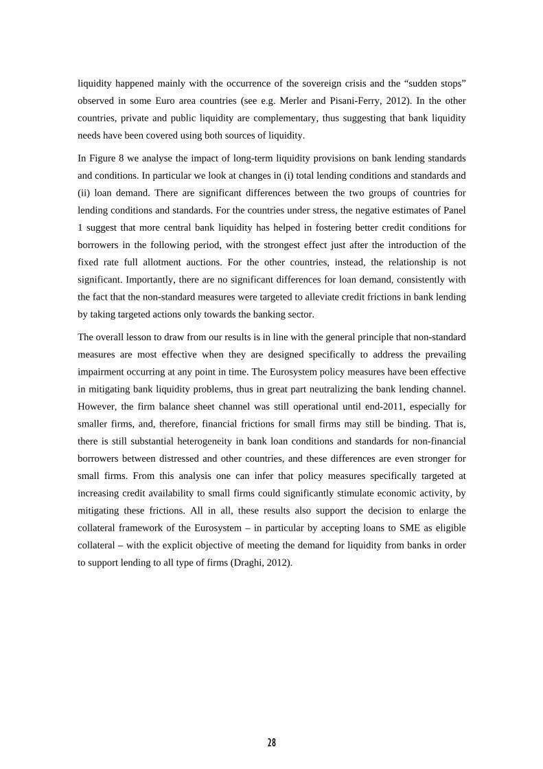
liquidity happened mainly with the occurrence of the sovereign crisis and the “sudden stops”

observed in some Euro area countries (see e.g. Merler and Pisani-Ferry, 2012). In the other

countries, private and public liquidity are complementary, thus suggesting that bank liquidity

needs have been covered using both sources of liquidity.

In Figure 8 we analyse the impact of long-term liquidity provisions on bank lending standards

and conditions. In particular we look at changes in (i) total lending conditions and standards and

(ii) loan demand. There are significant differences between the two groups of countries for

lending conditions and standards. For the countries under stress, the negative estimates of Panel

1 suggest that more central bank liquidity has helped in fostering better credit conditions for

borrowers in the following period, with the strongest effect just after the introduction of the

fixed rate full allotment auctions. For the other countries, instead, the relationship is not

significant. Importantly, there are no significant differences for loan demand, consistently with

the fact that the non-standard measures were targeted to alleviate credit frictions in bank lending

by taking targeted actions only towards the banking sector.

The overall lesson to draw from our results is in line with the general principle that non-standard

measures are most effective when they are designed specifically to address the prevailing

impairment occurring at any point in time. The Eurosystem policy measures have been effective

in mitigating bank liquidity problems, thus in great part neutralizing the bank lending channel.

However, the firm balance sheet channel was still operational until end-2011, especially for

smaller firms, and, therefore, financial frictions for small firms may still be binding. That is,

there is still substantial heterogeneity in bank loan conditions and standards for non-financial

borrowers between distressed and other countries, and these differences are even stronger for

small firms. From this analysis one can infer that policy measures specifically targeted at

increasing credit availability to small firms could significantly stimulate economic activity, by

mitigating these frictions. All in all, these results also support the decision to enlarge the

collateral framework of the Eurosystem – in particular by accepting loans to SME as eligible

collateral – with the explicit objective of meeting the demand for liquidity from banks in order

to support lending to all type of firms (Draghi, 2012).

28

5 CONCLUSIONS In this paper we have analysed how financial fragility has affected the monetary policy

transmission mechanism, in particular through the credit channel, placing emphasis on

heterogeneity at different levels. We look at the monetary policy transmission (i) in normal and

crisis times, (ii) for countries with different degrees of sovereign financial distress, (iii) for the

different channels of credit, and (iv) for banks and firms of different sizes.

By means of a reasoned narrative and of analytical tools that control for the dynamic

relationships between macro and financial variables and across a panel of 12 Euro area

countries, we have shown that the transmission mechanism of monetary policy has changed

with the crisis, with a strong amplification effect of the credit channel in countries under

sovereign stress. For these countries, the fragility of banks has been especially important in

2008-2009, whereas the firm/household balance sheet channel of monetary policy has been

significant during the whole period, especially for small firms.

With all the necessary caveats that such a non-structural analysis may entail, results indicate that

the effects of common monetary rates on GDP growth are significant and heterogeneous across

countries. We argue that the bank balance sheet problems might have been partly mitigated (and

the bank-lending channel partly “neutralized”) by the ECB interventions – which have targeted

almost exclusively banks’ liquidity – while the non-financial borrower balance sheet channel is

still significant, especially in financially distressed countries. For this group of countries, the

results suggest that more central bank liquidity has helped in fostering better credit conditions

for borrowers. However, our results also suggest that the policy framework until the end of 2011

might have fall short of increasing credit availability for small firms especially in distressed

countries. This in turn would support the complementary policy actions that have taken place

after the period analyzed in this paper, in particular the 3-year LTROs and the enlargement of

the collateral framework to include loans to SMEs as eligible collateral for central bank

operations. The latter was targeted precisely to address the problem of credit availability for

SMEs.

29

REFERENCES Adrian, T., and H. S. Shin. 2011. “Financial Intermediaries and Monetary Economics.” In

Handbook of Monetary Economics, ed. B.Friedman and M. Woodford. Amsterdam: Elsevier.

Allen, F, Chui, M., and A. Maddaloni, A. 2004. “Financial Systems in Europe, the U.S.A. and

Asia.” Oxford Review of Economic Policy 20(4):490-508.

Bachmann, R. and E. Sims. 2012. “Confidence and the Transmission of Government Spending

Shocks,” Journal of Monetary Economics 59:235–249

Bernanke, B. S. 2007. “The Financial Accelerator and the Credit Channel.” Remarks - Credit

Channel of Monetary Policy in the Twenty-first Century, Board of Governors of the U.S.

Federal Reserve System.

Bernanke, B. S., and Gertler, M. 1995. “Inside the Black Box: The Credit Channel of Monetary

Policy Transmission.” Journal of Economic Perspectives 9(4):27-48.

Canova, F. and M. Ciccarelli. 2009. “Estimating multi-country models”, International Economic

Review 50(3):929-959.

Ciccarelli, M., A. Maddaloni and J.L. Peydró. 2011. “Trusting the Bankers: A New Look at the

Credit Channel of Monetary Policy,” mimeo. Earlier draft published as ECB WP no. 1228.

Christiano, L. J., M. Eichenbaum, and C. L. Evans. 2000. “Monetary policy shocks: what have

we learned and to what end?” In Handbook of Macroeconomics, ed. J.Taylor and M. Woodford.

Amsterdam: Elsevier.

Christiano, L. J., M. Eichenbaum, and C. L. Evans. 1996. “The Effects of Monetary Policy

Shocks: Evidence From the Flow of Funds,” Review of Economics and Statistics.

Darracq Paries, M. and R.A. De Santis, 2013. “A Non-Standard Monetary Policy Shock: The ECB's 3-Year

LTROs and the Shift in Credit Supply”, ECB Working Paper, forthcoming.

Draghi, M. 2012. Transcript of the ECB Press Conference, 5 July.

Dudley, W., and J. Hatzius. 2000. “The Goldman Sachs Financial Conditions Index: The Right

Tool for a New Monetary Policy Regime.” Global Economics Paper No. 44.

Dudley, W., J. Hatzius, and E. McKelvey. 2005. “Financial Conditions Need to Tighten Further.

US Economics Analyst.” Goldman Sachs Economic Research.

Gertler, M., and P. Karadi. 2011. “A Model of Unconventional Monetary Policy.” Journal of

Monetary Economics 58: 17-34.

30

Gertler, M., and S. Gilchrist. 1994. “Monetary Policy, Business Cycles, and the Behavior of

Small Manufacturing Firms,” Quarterly Journal of Economics, 109:309-40.

Gertler, M., and Kiyotaki, N. 2010. “Financial Intermediation and Credit Policy in Business

Cycle Analysis.” Handbook of Monetary Economics, ed. B.Friedman and M. Woodford.

Amsterdam: Elsevier.

Jiménez, G., S. Ongena, J.-L. Peydró, and J. Saurina. 2012. “Credit Supply and Monetary

Policy: Identifying the Bank Balance-Sheet Channel with Loan Applications.” American

Economic Review August.

Kashyap, A. K., and J. C. Stein. 2000. “What Do a Million Observations on Banks Say About

the Transmission of Monetary Policy? American Economic Review 90(3):407-28.

Lenza, M., H. Pill, and L. Reichlin. 2010. “Monetary policy in exceptional times,” Economic

Policy 62, pp. 295-339.

Maddaloni, A., and J.-L. Peydró. 2011.“Bank Risk-Taking, Securitization, Supervision, and

Low Interest Rates: Evidence from the Euro Area and the U.S. Lending Standards.” Review of

Financial Studies 24:2121-2165.

Merler, S. and J. Pisani-Ferri. 2012. “Sudden stops in the euro area,” Bruegel Policy

Contribution, March.

Mishkin, F. S. 1977. “What Depressed the Consumer? The Household Balance Sheet and the

1973-75 Recession.” Brookings Papers on Economic Activity 1:123-164.

Mishkin, F. S. 1978. “The Household Balance Sheet and the Great Depression.” Journal of

Economic History 38:918-937.

Peersman, G. 2011. “Macroeconomic effects of unconventional monetary policy in the euro

area.” ECB Working Paper no. 1397.

Praet, P. 2012. “Heterogeneity in a monetary union: What have we learned?” Speech given at

the conference “The ECB and its watchers” in Frankfurt on 15 June.

Rubio-Ramirez, J.F., D.F. Waggoner and T. Zha (2010). ‘Structural vector autoregressions:

theory or identification and algorithms for inference’, Review of Economic Studies, 77(2),665-

96.

Soares, C. and P. M. M. Rodrigues. 2011. “Determinants of the EONIA spread and the financial

crisis,” Banco de Portugal Working Paper 12/2011.

Trichet, J. C. 2009. “The ECB's enhanced credit support,” keynote address at the University of

Munich, 13 July.

31

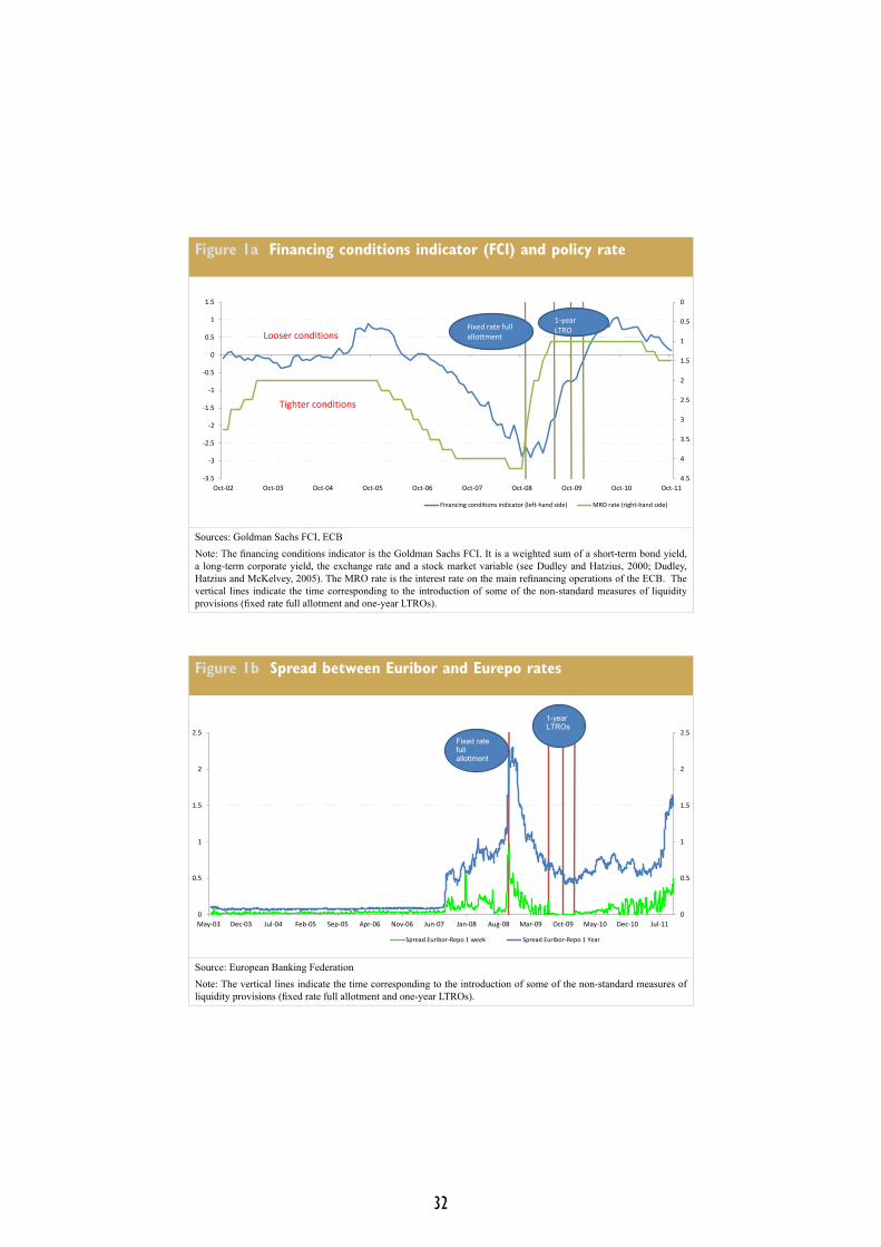
Figure 1a Financing conditions indicator (FCI) and policy rate

0

0.5

1

1.5

2

2.5

3

3.5

4

4.5-3.5

-3

-2.5

-2

-1.5

-1

-0.5

0

0.5

1

1.5

Oct-02 Oct-03 Oct-04 Oct-05 Oct-06 Oct-07 Oct-08 Oct-09 Oct-10 Oct-11

Financing conditions indicator (left-hand side) MRO rate (right-hand side)

Looser conditions1-year LTROFixed rate full

allottment

Tighter conditions

Sources: Goldman Sachs FCI, ECBNote: The financing conditions indicator is the Goldman Sachs FCI. It is a weighted sum of a short-term bond yield, a long-term corporate yield, the exchange rate and a stock market variable (see Dudley and Hatzius, 2000; Dudley, Hatzius and McKelvey, 2005). The MRO rate is the interest rate on the main refinancing operations of the ECB. The vertical lines indicate the time corresponding to the introduction of some of the non-standard measures of liquidity provisions (fixed rate full allotment and one-year LTROs).

Figure 1b Spread between Euribor and Eurepo rates

0

0.5

1

1.5

2

2.5

0

0.5

1

1.5

2

2.5

May-03 Dec-03 Jul-04 Feb-05 Sep-05 Apr-06 Nov-06 Jun-07 Jan-08 Aug-08 Mar-09 Oct-09 May-10 Dec-10 Jul-11

Spread Euribor-Repo 1 week Spread Euribor-Repo 1 Year

1-year LTROs

Fixed ratefull allottment

Source: European Banking FederationNote: The vertical lines indicate the time corresponding to the introduction of some of the non-standard measures of liquidity provisions (fixed rate full allotment and one-year LTROs).

32

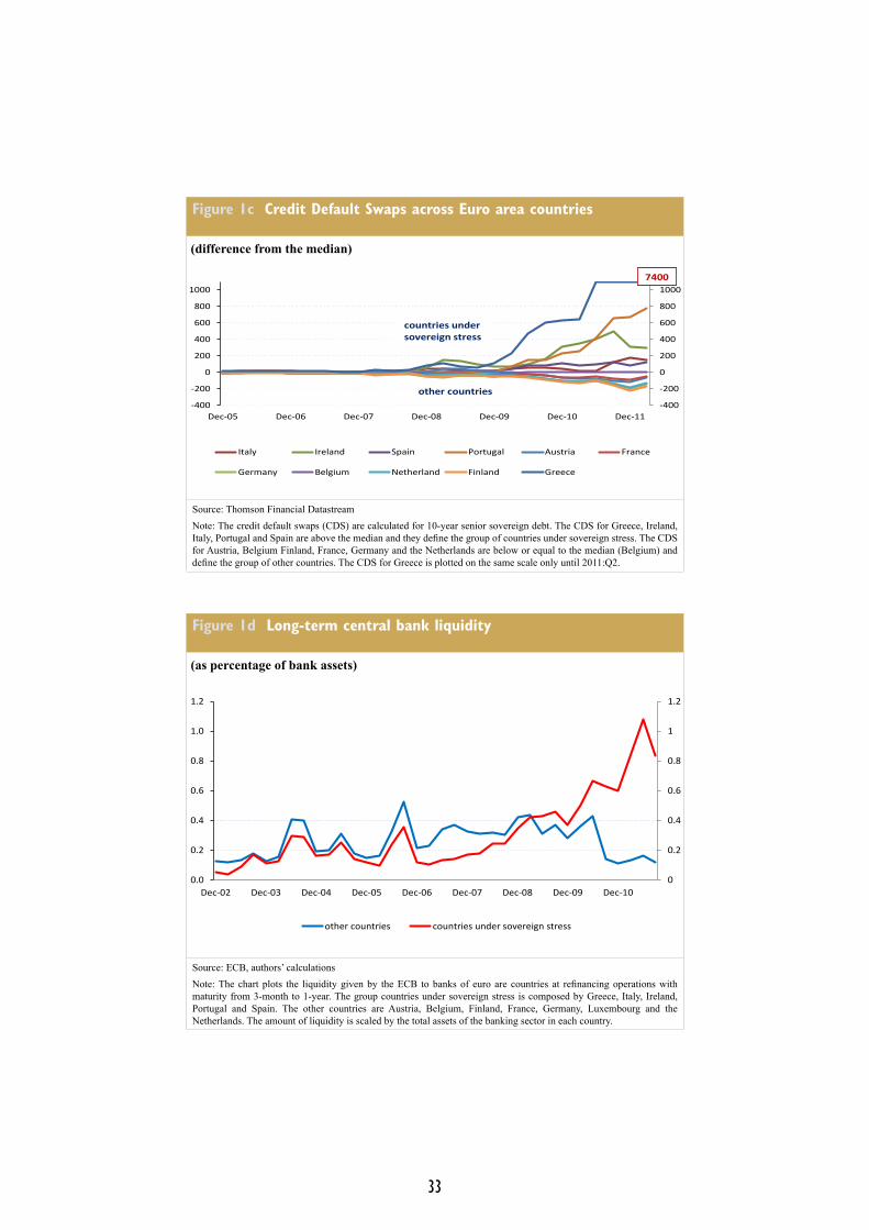
Figure 1c Credit Default Swaps across Euro area countries

(difference from the median)

-400

-200

0

200

400

600

800

1000

-400

-200

0

200

400

600

800

1000

Dec-05 Dec-06 Dec-07 Dec-08 Dec-09 Dec-10 Dec-11

Italy Ireland Spain Portugal Austria France

Germany Belgium Netherland Finland Greece

7400

countries under sovereign stress

7400

other countries

7400

Source: Thomson Financial DatastreamNote: The credit default swaps (CDS) are calculated for 10-year senior sovereign debt. The CDS for Greece, Ireland, Italy, Portugal and Spain are above the median and they define the group of countries under sovereign stress. The CDS for Austria, Belgium Finland, France, Germany and the Netherlands are below or equal to the median (Belgium) and define the group of other countries. The CDS for Greece is plotted on the same scale only until 2011:Q2.

Figure 1d Long-term central bank liquidity

(as percentage of bank assets)

0

0.2

0.4

0.6

0.8

1

1.2

0.0

0.2

0.4

0.6

0.8

1.0

1.2

Dec-02 Dec-03 Dec-04 Dec-05 Dec-06 Dec-07 Dec-08 Dec-09 Dec-10

other countries countries under sovereign stress

Source: ECB, authors’ calculationsNote: The chart plots the liquidity given by the ECB to banks of euro are countries at refinancing operations with maturity from 3-month to 1-year. The group countries under sovereign stress is composed by Greece, Italy, Ireland, Portugal and Spain. The other countries are Austria, Belgium, Finland, France, Germany, Luxembourg and the Netherlands. The amount of liquidity is scaled by the total assets of the banking sector in each country.

33

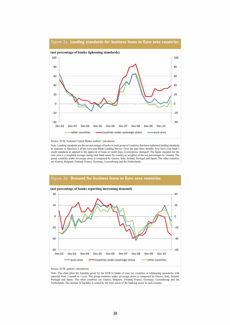
Figure 2a Lending standards for business loans in Euro area countries

(net percentage of banks tightening standards)

-40

-20

0

20

40

60

80

100

-40

-20

0

20

40

60

80

100

Dec-02 Dec-03 Dec-04 Dec-05 Dec-06 Dec-07 Dec-08 Dec-09 Dec-10

other countries countries under sovereign stress euro area

Source: ECB, National Central Banks, authors’ calculationNote: Lending standards are the net percentage of banks in each group of countries that have tightened lending standards in response to Question 1 of the euro area Bank Lending Survey: Over the past three months, how have your bank’s credit standards as applied to the approval of loans or credit lines to enterprises changed? The figure reported for the euro area is a weighted average (using total bank assets by country as weights) of the net percentages by country. The group countries under sovereign stress is composed by Greece, Italy, Ireland, Portugal and Spain. The other countries are Austria, Belgium, Finland, France, Germany, Luxembourg and the Netherlands.

Figure 2b Demand for business loans in Euro area countries

(net percentage of banks reporting increasing demand)

-60

-40

-20

0

20

40

-60

-40

-20

0

20

40

Dec-02 Dec-03 Dec-04 Dec-05 Dec-06 Dec-07 Dec-08 Dec-09 Dec-10

euro area countries under sovereign stress other countries

Source: ECB, authors’ calculationsNote: The chart plots the liquidity given by the ECB to banks of euro are countries at refinancing operations with maturity from 3-month to 1-year. The group countries under sovereign stress is composed by Greece, Italy, Ireland, Portugal and Spain. The other countries are Austria, Belgium, Finland, France, Germany, Luxembourg and the Netherlands. The amount of liquidity is scaled by the total assets of the banking sector in each country.

34

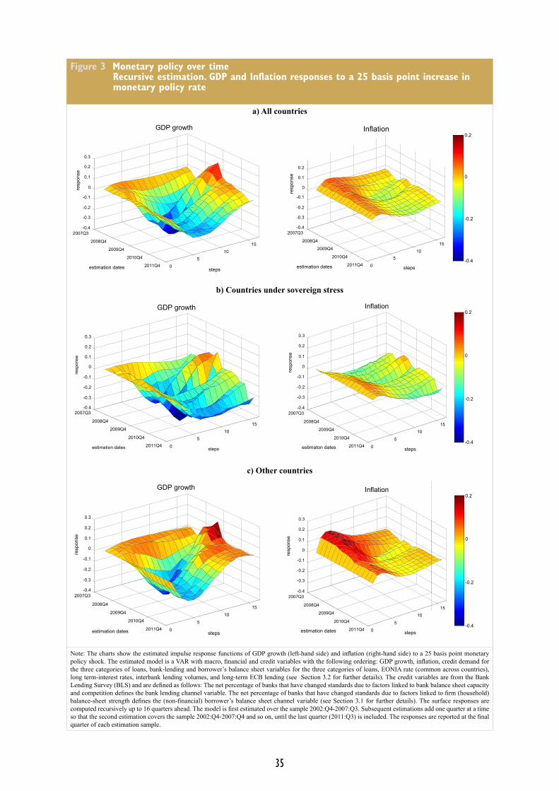
Figure 3 Monetary policy over timeRecursive estimation. GDP and Inflation responses to a 25 basis point increase in monetary policy rate

a) All countries

0

5

10

15

2007Q3

2008Q4

2009Q4

2010Q4

2011Q4

-0.4

-0.3

-0.2

-0.1

0

0.1

0.2

0.3

steps

GDP growth

estimation dates

resp

onse

0

510

15

2007Q3

2008Q4

2009Q4

2010Q4

2011Q4

-0.4

-0.3

-0.2

-0.1

0

0.1

0.2

steps

Inflation

estimation dates

resp

onse

-0.4

-0.2

0

0.2

b) Countries under sovereign stress

0

510

15

2007Q3

2008Q4

2009Q4

2010Q4

2011Q4

-0.4

-0.3

-0.2

-0.1

0

0.1

0.2

0.3

steps

GDP growth

estimation dates

resp

onse

0

5

10

15

2007Q3

2008Q4

2009Q4

2010Q4

2011Q4

-0.4

-0.3

-0.2

-0.1

0

0.1

0.2

0.3

steps

Inflation

estimaton dates

resp

onse

-0.4

-0.2

0

0.2

c) Other countries

0

5

10

15

2007Q3

2008Q4

2009Q4

2010Q4

2011Q4

-0.4

-0.3

-0.2

-0.1

0

0.1

0.2

0.3

steps

GDP growth

estimation dates

resp

onse

0

5

10

15

2007Q3

2008Q4

2009Q4

2010Q4

2011Q4

-0.4

-0.3

-0.2

-0.1

0

0.1

0.2

0.3

steps

Inflation

estimation dates

resp

onse

-0.4

-0.2

0

0.2

Note: The charts show the estimated impulse response functions of GDP growth (left-hand side) and inflation (right-hand side) to a 25 basis point monetary policy shock. The estimated model is a VAR with macro, financial and credit variables with the following ordering: GDP growth, inflation, credit demand for the three categories of loans, bank-lending and borrower’s balance sheet variables for the three categories of loans, EONIA rate (common across countries), long term-interest rates, interbank lending volumes, and long-term ECB lending (see Section 3.2 for further details). The credit variables are from the Bank Lending Survey (BLS) and are defined as follows: The net percentage of banks that have changed standards due to factors linked to bank balance sheet capacity and competition defines the bank lending channel variable. The net percentage of banks that have changed standards due to factors linked to firm (household) balance-sheet strength defines the (non-financial) borrower’s balance sheet channel variable (see Section 3.1 for further details). The surface responses are computed recursively up to 16 quarters ahead. The model is first estimated over the sample 2002:Q4-2007:Q3. Subsequent estimations add one quarter at a time so that the second estimation covers the sample 2002:Q4-2007:Q4 and so on, until the last quarter (2011:Q3) is included. The responses are reported at the final quarter of each estimation sample.

35

Figure 4 Monetary policy and the credit channel - Recursive counterfactual analysis. GDP responses to a 25 basis point increase in monetary policy rate

a) Countries under sovereign stress

total effect effect without the channel

Note: The charts show the estimated impulse response functions of GDP growth to a 25 basis point monetary policy shock. The responses are computed recursively. The model is first estimated over the sample 2002:Q4-2007:Q3. Subsequent estimations add one quarter at a time so that the second estimation covers the sample 2002:Q4-2007:Q4 and so on, until the last quarter (2011:Q3) is included. The responses are shown at selected quarters. The black line is the median response estimated from a full system (VAR with 15 variables with the following ordering: GDP growth, inflation, credit demand for the three categories of loans, bank-lending and borrower’s balance sheet variables for the three categories of loans, EONIA rate (common across countries), long term-interest rates, interbank lending volumes, and long-term ECB lending, see also Section 3.2). The blue area is a 68% Bayesian credible set around this median. The red line is the response obtained when closing down the broad credit channel (left-hand side) or the credit demand channel (right-hand side). The difference between the black and the red line is the median amplification effect due to the broad credit or the credit demand channel. The counterfactuals are constructed by using a hypothetical sequence of shocks to the relevant credit variables (the broad credit channel variables defined as the net percentage of banks that have changed lending conditions and standards that banks apply to borrowers and the credit demand channel variables defined as the net percentage of banks reporting an increase in the demand for loans. These credit variables are from the Bank Lending Survey (BLS), see also Section 3.1). Results are reported separately for countries under sovereign stress (panel A) and for other countries (panel B).

2007Q3

2008Q4

2009Q4

2010Q3

2011Q3

Broad credit channel Credit demand channel

36

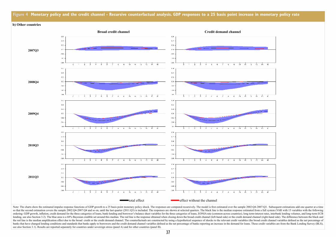
Figure 4 Monetary policy and the credit channel - Recursive counterfactual analysis. GDP responses to a 25 basis point increase in monetary policy rate

b) Other countries

total effect effect without the channel

Note: The charts show the estimated impulse response functions of GDP growth to a 25 basis point monetary policy shock. The responses are computed recursively. The model is first estimated over the sample 2002:Q4-2007:Q3. Subsequent estimations add one quarter at a time so that the second estimation covers the sample 2002:Q4-2007:Q4 and so on, until the last quarter (2011:Q3) is included. The responses are shown at selected quarters. The black line is the median response estimated from a full system (VAR with 15 variables with the following ordering: GDP growth, inflation, credit demand for the three categories of loans, bank-lending and borrower’s balance sheet variables for the three categories of loans, EONIA rate (common across countries), long term-interest rates, interbank lending volumes, and long-term ECB lending, see also Section 3.2). The blue area is a 68% Bayesian credible set around this median. The red line is the response obtained when closing down the broad credit channel (left-hand side) or the credit demand channel (right-hand side). The difference between the black and the red line is the median amplification effect due to the broad credit or the credit demand channel. The counterfactuals are constructed by using a hypothetical sequence of shocks to the relevant credit variables (the broad credit channel variables defined as the net percentage of banks that have changed lending conditions and standards that banks apply to borrowers and the credit demand channel variables defined as the net percentage of banks reporting an increase in the demand for loans. These credit variables are from the Bank Lending Survey (BLS), see also Section 3.1). Results are reported separately for countries under sovereign stress (panel A) and for other countries (panel B).

2007Q3

2008Q4

2009Q4

2010Q3

2011Q3

Broad credit channel Credit demand channel

37

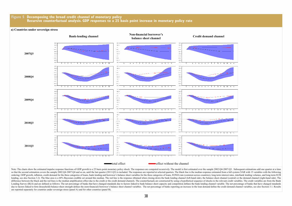
Figure 5 Decomposing the broad credit channel of monetary policyRecursive counterfactual analysis. GDP responses to a 25 basis point increase in monetary policy rate

a) Countries under sovereign stress

total effect effect without the channel

Note: The charts show the estimated impulse response functions of GDP growth to a 25 basis point monetary policy shock. The responses are computed recursively. The model is first estimated over the sample 2002:Q4-2007:Q3. Subsequent estimations add one quarter at a time so that the second estimation covers the sample 2002:Q4-2007:Q4 and so on, until the last quarter (2011:Q3) is included. The responses are reported at selected quarters. The black line is the median response estimated from a full system (VAR with 15 variables with the following ordering: GDP growth, inflation, credit demand for the three categories of loans, bank-lending and borrower’s balance sheet variables for the three categories of loans, EONIA rate (common across countries), long term-interest rates, interbank lending volumes, and long-term ECB lending, see also Section 3.2). The blue area is a 68% Bayesian credible set around this median. The red line is the response obtained when closing down the bank lending channel (left-hand side), the balance sheet channel (central) or the demand channel (right-hand side). The difference between the black and the red lines is the median amplification effect due to the credit or the credit demand channels. The counterfactuals are constructed by using a hypothetical sequence of shocks to the relevant credit variables. The credit variables are from the Bank Lending Survey (BLS) and are defined as follows: The net percentage of banks that have changed standards due to factors linked to bank balance sheet capacity and competition defines the bank lending channel variable. The net percentage of banks that have changed standards due to factors linked to firm (household) balance-sheet strength defines the (non-financial) borrower’s balance sheet channel variables. The net percentage of banks reporting an increase in the loan demand define the credit demand channel variables, see also Section 3.1. Results are reported separately for countries under sovereign stress (panel A) and for other countries (panel B).

Bank-lending channel Non-financial borrower’s balance sheet channel Credit demand channel

2007Q3

2008Q4

2009Q4

2010Q3

2011Q3

38

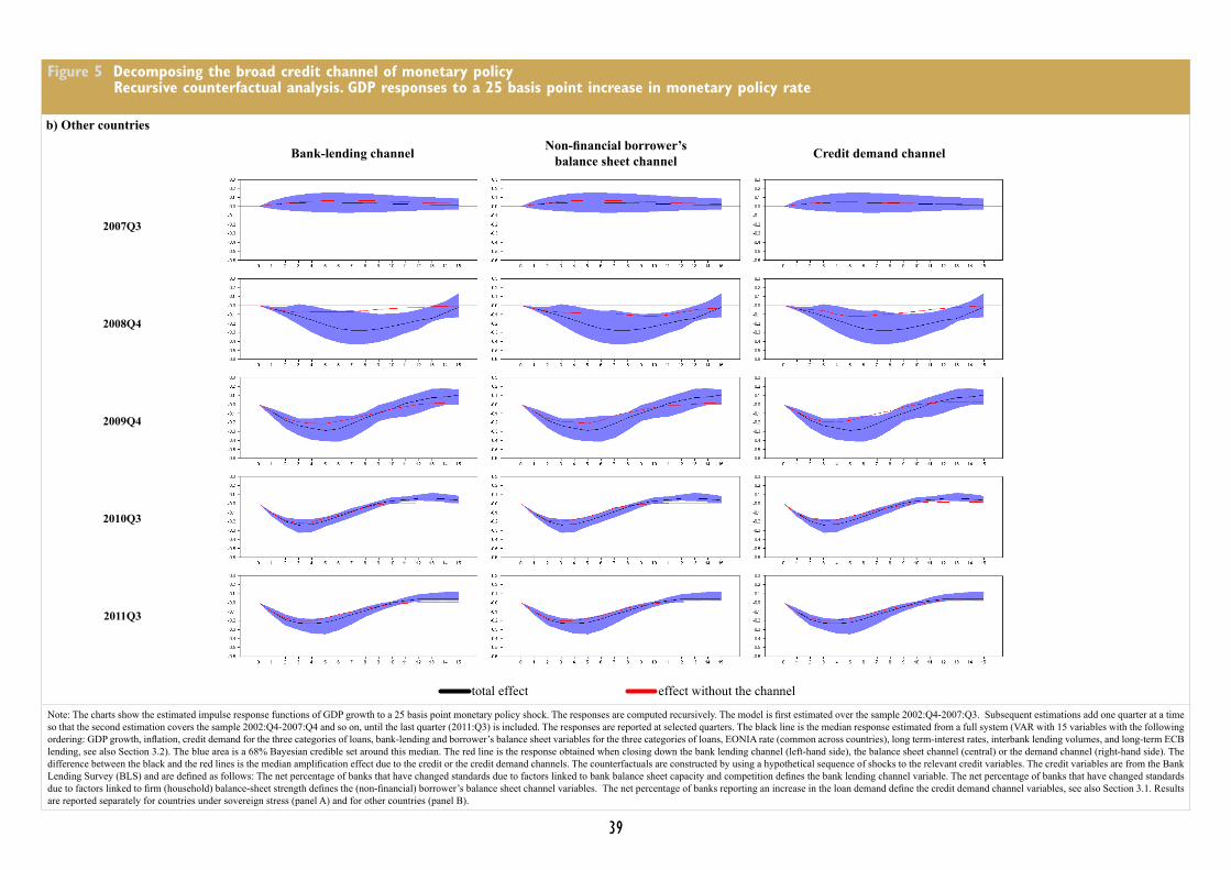
Figure 5 Decomposing the broad credit channel of monetary policyRecursive counterfactual analysis. GDP responses to a 25 basis point increase in monetary policy rate

b) Other countries

total effect effect without the channel

Note: The charts show the estimated impulse response functions of GDP growth to a 25 basis point monetary policy shock. The responses are computed recursively. The model is first estimated over the sample 2002:Q4-2007:Q3. Subsequent estimations add one quarter at a time so that the second estimation covers the sample 2002:Q4-2007:Q4 and so on, until the last quarter (2011:Q3) is included. The responses are reported at selected quarters. The black line is the median response estimated from a full system (VAR with 15 variables with the following ordering: GDP growth, inflation, credit demand for the three categories of loans, bank-lending and borrower’s balance sheet variables for the three categories of loans, EONIA rate (common across countries), long term-interest rates, interbank lending volumes, and long-term ECB lending, see also Section 3.2). The blue area is a 68% Bayesian credible set around this median. The red line is the response obtained when closing down the bank lending channel (left-hand side), the balance sheet channel (central) or the demand channel (right-hand side). The difference between the black and the red lines is the median amplification effect due to the credit or the credit demand channels. The counterfactuals are constructed by using a hypothetical sequence of shocks to the relevant credit variables. The credit variables are from the Bank Lending Survey (BLS) and are defined as follows: The net percentage of banks that have changed standards due to factors linked to bank balance sheet capacity and competition defines the bank lending channel variable. The net percentage of banks that have changed standards due to factors linked to firm (household) balance-sheet strength defines the (non-financial) borrower’s balance sheet channel variables. The net percentage of banks reporting an increase in the loan demand define the credit demand channel variables, see also Section 3.1. Results are reported separately for countries under sovereign stress (panel A) and for other countries (panel B).

Bank-lending channel Non-financial borrower’s balance sheet channel Credit demand channel

2007Q3

2008Q4

2009Q4

2010Q3

2011Q3

39

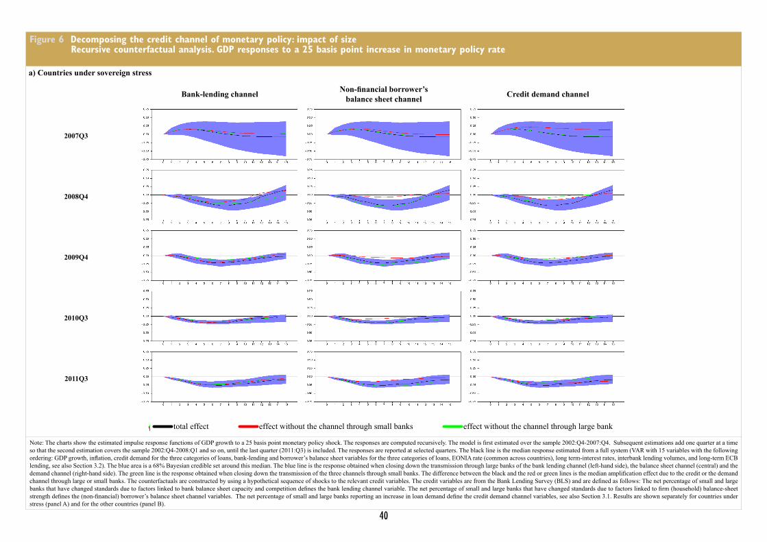
Figure 6 Decomposing the credit channel of monetary policy: impact of size Recursive counterfactual analysis. GDP responses to a 25 basis point increase in monetary policy rate

a) Countries under sovereign stress

total effect effect without the channel through small banks effect without the channel through large bank

Note: The charts show the estimated impulse response functions of GDP growth to a 25 basis point monetary policy shock. The responses are computed recursively. The model is first estimated over the sample 2002:Q4-2007:Q4. Subsequent estimations add one quarter at a time so that the second estimation covers the sample 2002:Q4-2008:Q1 and so on, until the last quarter (2011:Q3) is included. The responses are reported at selected quarters. The black line is the median response estimated from a full system (VAR with 15 variables with the following ordering: GDP growth, inflation, credit demand for the three categories of loans, bank-lending and borrower’s balance sheet variables for the three categories of loans, EONIA rate (common across countries), long term-interest rates, interbank lending volumes, and long-term ECB lending, see also Section 3.2). The blue area is a 68% Bayesian credible set around this median. The blue line is the response obtained when closing down the transmission through large banks of the bank lending channel (left-hand side), the balance sheet channel (central) and the demand channel (right-hand side). The green line is the response obtained when closing down the transmission of the three channels through small banks. The difference between the black and the red or green lines is the median amplification effect due to the credit or the demand channel through large or small banks. The counterfactuals are constructed by using a hypothetical sequence of shocks to the relevant credit variables. The credit variables are from the Bank Lending Survey (BLS) and are defined as follows: The net percentage of small and large banks that have changed standards due to factors linked to bank balance sheet capacity and competition defines the bank lending channel variable. The net percentage of small and large banks that have changed standards due to factors linked to firm (household) balance-sheet strength defines the (non-financial) borrower’s balance sheet channel variables. The net percentage of small and large banks reporting an increase in loan demand define the credit demand channel variables, see also Section 3.1. Results are shown separately for countries under stress (panel A) and for the other countries (panel B).

Bank-lending channel Non-financial borrower’s balance sheet channel Credit demand channel

2007Q3

2008Q4

2009Q4

2010Q3

2011Q3

40

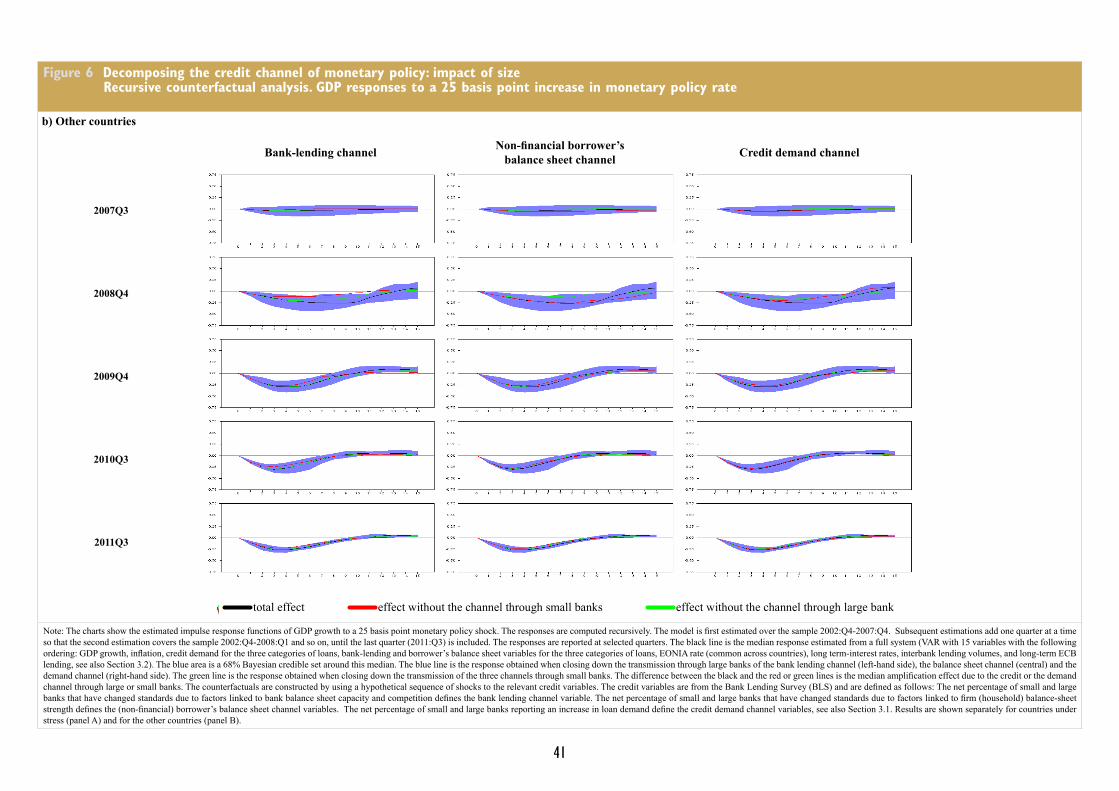
Figure 6 Decomposing the credit channel of monetary policy: impact of size Recursive counterfactual analysis. GDP responses to a 25 basis point increase in monetary policy rate

b) Other countries

total effect effect without the channel through small banks effect without the channel through large bank

Note: The charts show the estimated impulse response functions of GDP growth to a 25 basis point monetary policy shock. The responses are computed recursively. The model is first estimated over the sample 2002:Q4-2007:Q4. Subsequent estimations add one quarter at a time so that the second estimation covers the sample 2002:Q4-2008:Q1 and so on, until the last quarter (2011:Q3) is included. The responses are reported at selected quarters. The black line is the median response estimated from a full system (VAR with 15 variables with the following ordering: GDP growth, inflation, credit demand for the three categories of loans, bank-lending and borrower’s balance sheet variables for the three categories of loans, EONIA rate (common across countries), long term-interest rates, interbank lending volumes, and long-term ECB lending, see also Section 3.2). The blue area is a 68% Bayesian credible set around this median. The blue line is the response obtained when closing down the transmission through large banks of the bank lending channel (left-hand side), the balance sheet channel (central) and the demand channel (right-hand side). The green line is the response obtained when closing down the transmission of the three channels through small banks. The difference between the black and the red or green lines is the median amplification effect due to the credit or the demand channel through large or small banks. The counterfactuals are constructed by using a hypothetical sequence of shocks to the relevant credit variables. The credit variables are from the Bank Lending Survey (BLS) and are defined as follows: The net percentage of small and large banks that have changed standards due to factors linked to bank balance sheet capacity and competition defines the bank lending channel variable. The net percentage of small and large banks that have changed standards due to factors linked to firm (household) balance-sheet strength defines the (non-financial) borrower’s balance sheet channel variables. The net percentage of small and large banks reporting an increase in loan demand define the credit demand channel variables, see also Section 3.1. Results are shown separately for countries under stress (panel A) and for the other countries (panel B).

Bank-lending channel Non-financial borrower’s balance sheet channel Credit demand channel

2007Q3

2008Q4

2009Q4

2010Q3

2011Q3

41

Figure 7 Effects of interbank transactions on long-term central bank liquidity (LTRO)

Recursive panel estimates

-0.2

-0.1

0

0.1

0.2

0.3

0.4

Dec-07 Aug-08 Apr-09 Dec-09 Aug-10 Apr-11

countries under sovereign stress other countries

Fixed -rate fullallotment starts

Note: The chart reports the recursive estimates of the coefficients of the interbank transaction volumes (among the EONIA panel banks) in a regression where the left-hand side variable is the liquidity provided in the long term refinancing operations (LTROs) by the central bank. Additional control variables are: GDP growth, inflation, credit demand for the three categories of loans, bank-lending and borrower’s balance sheet variables for the three categories of loans, EONIA rate and long term-interest rates. All explanatory variables are lagged by one quarter. The red line is the estimated coefficient for the set of countries under stress; the blue line for the other countries. The dotted lines mark the 68% confidence interval.

42

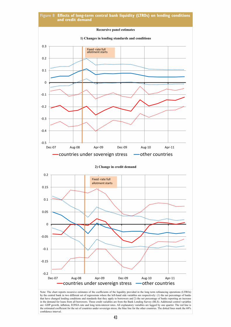
Figure 8 Effects of long-term central bank liquidity (LTROs) on lending conditions and credit demand

Recursive panel estimates

1) Changes in lending standards and conditions

-0.5

-0.4

-0.3

-0.2

-0.1

0

0.1

0.2

0.3

Dec-07 Aug-08 Apr-09 Dec-09 Aug-10 Apr-11

countries under sovereign stress other countries

Fixed -rate fullallotment starts

2) Change in credit demand

-0.2

-0.15

-0.1

-0.05

0

0.05

0.1

0.15

0.2

Dec-07 Aug-08 Apr-09 Dec-09 Aug-10 Apr-11

countries under sovereign stress other countries

Fixed -rate fullallotment starts

Note: The chart reports recursive estimates of the coefficients of the liquidity provided in the long term refinancing operations (LTROs) by the central bank in two different set of regressions where the left-hand side variables are respectively: (1) the net percentage of banks that have changed lending conditions and standards that they apply to borrowers and 2) the net percentage of banks reporting an increase in the demand for loans from all borrowers. These credit variables are from the Bank Lending Survey (BLS). Additional control variables are: GDP growth, inflation, EONIA rate and long term-interest rates. All explanatory variables are lagged by one quarter. The red line is the estimated coefficient for the set of countries under sovereign stress; the blue line for the other countries. The dotted lines mark the 68% confidence interval.

43

Table A.1 Data The Bank Lending Survey

Questions from the Survey and variables used in the analysis

Question Factors affecting decision Variables used in the analysis Measures

Lending conditions and standards

Over the past three months, how have your bank’s credit standards as applied to the approval of loans…

Broad credit channel variablefor: Net percentage is equal to the

difference between the sum of banks answering “tightened considerably” and “tightened somewhat” and the sum of banks answering “eased somewhat” and “eased considerably” in percentage of the total number of banks.

or credit lines to enterprises changed? (Q1)

business loans

to households for house purchase changed? (Q8)

mortgage loans

to households for consumer credit and other lending changed? (Q8)

consumer loans

Factors affecting lending conditions

Net percentage is equal to the difference between the sum of the banks answering “contributed considerably to tightening” and “contributed somewhat to tightening” and the sum of the banks answering “contributed somewhat to easing” and “contributed considerably to easing” in percentage of the total number of banks

Q2: Over the past three months, how have the following factors affected your bank’s credit standards as applied to the approval of loans or credit lines to enterprises?

A Costs of funds and [bank] balance sheet constraints

Costs related to your bank’s capital position

Bank lending channel variable is the average of the net percentage of banks answering A and B

Your bank’s ability to access market financing

Your bank’s liquidity position

B Pressure from competition [from banks and other financial intermediaries]

Competition from other banks

Q9: Over the past three months, how have the following factors affected your bank’s credit standards as applied to the approval of loans to households for house purchase?

Competition from non-banks

Competition from market financing

C Perception of risk Expectations regarding general economic activity

(non-financial) Borrower’s balance sheet channel variable is the average of the net percentage of banks answering C

Q11: Over the past three months, how have the following factors affected your bank’s credit standards as applied to the approval of consumer credit and other lending to households?

Industry or firm-specific outlook

Risk on the collateral demanded (for business and consumer loans)

Housing market prospects (for mortgage loans)

Creditworthiness of consumers (for consumer loans)

Demand for loans Credit demand variable for: Net percentage is equal to the difference between the sum of the banks answering “increased considerably” and “increased somewhat” and the sum of the banks answering “decreased somewhat” and “decreased considerably” in percentage of the total number of banks

Over the past three months, how has the demand for loans or credit lines to [enterprises (Q4), households (Q13)] changed at your bank, apart from normal seasonal fluctuations?

business loans

mortgage loans

consumer loans

Source: ECB and national central banks. See http://www.ecb.europa.eu/stats/money/surveys/lend/html/index.en.html for a full description of the surveyNote: Q* indicate the number of that question in the Bank Lending SurveyNote on confidentiality: some of the data are not publicly available, in particular the complete panel of responses from the BLS are the country level

AppEnDIx

Table A.2 Data, sources and transformations

Definition Source Sample Transformation

GDP Eurostat 2002:Q4-2011:Q3 year-on-year growth rateGDP deflator Economic Outlook (OECD) 2002:Q4-2011:Q3 year-on-year growth rateInterbank lending volumes European Banking Federation (EBF) 2002:Q4-2011:Q3 year-on-year change(EONIA panel banks)

EONIA rates ECB: Euro Interbank Offered Rate 2002:Q4-2011:Q3 year-on-year changeLong term government bond yields MEI : Main Economic Indicators (OECD) 2002:Q4-2011:Q3 year-on-year changeLong-term central bank liquidity ECB 2002:Q4-2011:Q3 liquidity over bank total assets by country(3-month to 1-year maturity)

Bank total assets ECB 2002:Q4-2011:Q3 levelNote on confidentiality: Some of the data are not publicly available, in particular the interbank lending volumes of the EONIA panel banks and the EONIA rates.

44

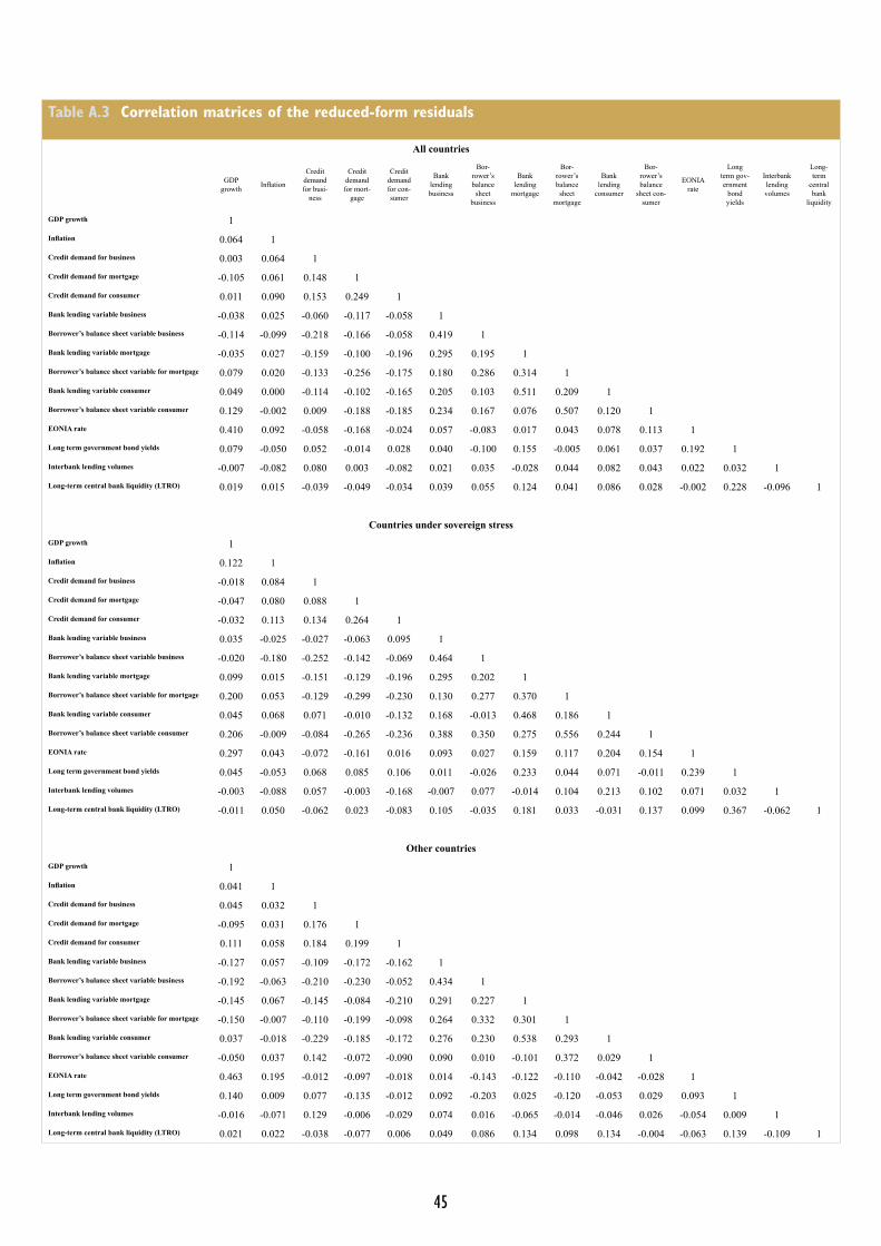
Table A.3 Correlation matrices of the reduced-form residuals

All countries

GDP growth Inflation

Credit demand for busi-

ness

Credit demand for mort-

gage

Credit demand for con-sumer

Bank lending business

Bor-rower’s balance sheet

business

Bank lending

mortgage

Bor-rower’s balance sheet

mortgage

Bank lending

consumer

Bor-rower’s balance

sheet con-sumer

EONIA rate

Long term gov-ernment

bond yields

Interbank lending volumes

Long-term

central bank

liquidity

GDP growth 1Inflation 0.064 1Credit demand for business 0.003 0.064 1Credit demand for mortgage -0.105 0.061 0.148 1Credit demand for consumer 0.011 0.090 0.153 0.249 1Bank lending variable business -0.038 0.025 -0.060 -0.117 -0.058 1Borrower’s balance sheet variable business -0.114 -0.099 -0.218 -0.166 -0.058 0.419 1Bank lending variable mortgage -0.035 0.027 -0.159 -0.100 -0.196 0.295 0.195 1Borrower’s balance sheet variable for mortgage 0.079 0.020 -0.133 -0.256 -0.175 0.180 0.286 0.314 1Bank lending variable consumer 0.049 0.000 -0.114 -0.102 -0.165 0.205 0.103 0.511 0.209 1Borrower’s balance sheet variable consumer 0.129 -0.002 0.009 -0.188 -0.185 0.234 0.167 0.076 0.507 0.120 1EONIA rate 0.410 0.092 -0.058 -0.168 -0.024 0.057 -0.083 0.017 0.043 0.078 0.113 1Long term government bond yields 0.079 -0.050 0.052 -0.014 0.028 0.040 -0.100 0.155 -0.005 0.061 0.037 0.192 1Interbank lending volumes -0.007 -0.082 0.080 0.003 -0.082 0.021 0.035 -0.028 0.044 0.082 0.043 0.022 0.032 1Long-term central bank liquidity (LTRO) 0.019 0.015 -0.039 -0.049 -0.034 0.039 0.055 0.124 0.041 0.086 0.028 -0.002 0.228 -0.096 1

Countries under sovereign stressGDP growth 1Inflation 0.122 1Credit demand for business -0.018 0.084 1Credit demand for mortgage -0.047 0.080 0.088 1Credit demand for consumer -0.032 0.113 0.134 0.264 1Bank lending variable business 0.035 -0.025 -0.027 -0.063 0.095 1Borrower’s balance sheet variable business -0.020 -0.180 -0.252 -0.142 -0.069 0.464 1Bank lending variable mortgage 0.099 0.015 -0.151 -0.129 -0.196 0.295 0.202 1Borrower’s balance sheet variable for mortgage 0.200 0.053 -0.129 -0.299 -0.230 0.130 0.277 0.370 1Bank lending variable consumer 0.045 0.068 0.071 -0.010 -0.132 0.168 -0.013 0.468 0.186 1Borrower’s balance sheet variable consumer 0.206 -0.009 -0.084 -0.265 -0.236 0.388 0.350 0.275 0.556 0.244 1EONIA rate 0.297 0.043 -0.072 -0.161 0.016 0.093 0.027 0.159 0.117 0.204 0.154 1Long term government bond yields 0.045 -0.053 0.068 0.085 0.106 0.011 -0.026 0.233 0.044 0.071 -0.011 0.239 1Interbank lending volumes -0.003 -0.088 0.057 -0.003 -0.168 -0.007 0.077 -0.014 0.104 0.213 0.102 0.071 0.032 1Long-term central bank liquidity (LTRO) -0.011 0.050 -0.062 0.023 -0.083 0.105 -0.035 0.181 0.033 -0.031 0.137 0.099 0.367 -0.062 1

Other countries GDP growth 1Inflation 0.041 1Credit demand for business 0.045 0.032 1Credit demand for mortgage -0.095 0.031 0.176 1Credit demand for consumer 0.111 0.058 0.184 0.199 1Bank lending variable business -0.127 0.057 -0.109 -0.172 -0.162 1Borrower’s balance sheet variable business -0.192 -0.063 -0.210 -0.230 -0.052 0.434 1Bank lending variable mortgage -0.145 0.067 -0.145 -0.084 -0.210 0.291 0.227 1Borrower’s balance sheet variable for mortgage -0.150 -0.007 -0.110 -0.199 -0.098 0.264 0.332 0.301 1Bank lending variable consumer 0.037 -0.018 -0.229 -0.185 -0.172 0.276 0.230 0.538 0.293 1Borrower’s balance sheet variable consumer -0.050 0.037 0.142 -0.072 -0.090 0.090 0.010 -0.101 0.372 0.029 1EONIA rate 0.463 0.195 -0.012 -0.097 -0.018 0.014 -0.143 -0.122 -0.110 -0.042 -0.028 1Long term government bond yields 0.140 0.009 0.077 -0.135 -0.012 0.092 -0.203 0.025 -0.120 -0.053 0.029 0.093 1Interbank lending volumes -0.016 -0.071 0.129 -0.006 -0.029 0.074 0.016 -0.065 -0.014 -0.046 0.026 -0.054 0.009 1Long-term central bank liquidity (LTRO) 0.021 0.022 -0.038 -0.077 0.006 0.049 0.086 0.134 0.098 0.134 -0.004 -0.063 0.139 -0.109 1

45

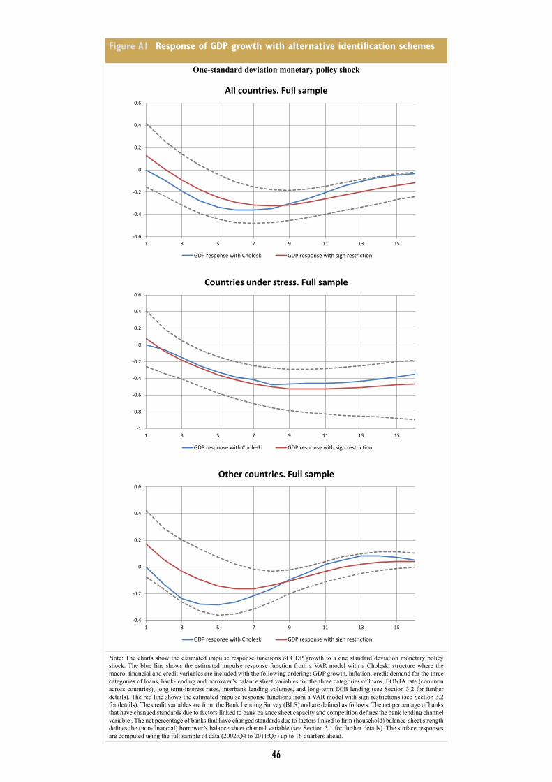
Figure A1 Response of GDP growth with alternative identification schemes

One-standard deviation monetary policy shock

-0.6

-0.4

-0.2

0

0.2

0.4

0.6

1 3 5 7 9 11 13 15

All countries. Full sample

GDP response with Choleski GDP response with sign restriction

-1

-0.8

-0.6

-0.4

-0.2

0

0.2

0.4

0.6

1 3 5 7 9 11 13 15

Countries under stress. Full sample

GDP response with Choleski GDP response with sign restriction

-0.4

-0.2

0

0.2

0.4

0.6

1 3 5 7 9 11 13 15

Other countries. Full sample

GDP response with Choleski GDP response with sign restriction

Note: The charts show the estimated impulse response functions of GDP growth to a one standard deviation monetary policy shock. The blue line shows the estimated impulse response function from a VAR model with a Choleski structure where the macro, financial and credit variables are included with the following ordering: GDP growth, inflation, credit demand for the three categories of loans, bank-lending and borrower’s balance sheet variables for the three categories of loans, EONIA rate (common across countries), long term-interest rates, interbank lending volumes, and long-term ECB lending (see Section 3.2 for further details). The red line shows the estimated impulse response functions from a VAR model with sign restrictions (see Section 3.2 for details). The credit variables are from the Bank Lending Survey (BLS) and are defined as follows: The net percentage of banks that have changed standards due to factors linked to bank balance sheet capacity and competition defines the bank lending channel variable . The net percentage of banks that have changed standards due to factors linked to firm (household) balance-sheet strength defines the (non-financial) borrower’s balance sheet channel variable (see Section 3.1 for further details). The surface responses are computed using the full sample of data (2002:Q4 to 2011:Q3) up to 16 quarters ahead.

46