heterogeneous treatment e ects with mismeasured endogenous
TRANSCRIPT

Heterogeneous Treatment Effects with
Mismeasured Endogenous Treatment∗
Takuya Ura
Department of Economics
Duke University
Job Market Paper
November 25, 2015
The latest version is found in http://sites.duke.edu/takuyaura/.
Abstract
This paper studies the identifying power of an instrumental variable in the nonparametric heteroge-
neous treatment effect framework when a binary treatment variable is mismeasured and endogenous. I
characterize the sharp identified set for the local average treatment effect under the following two as-
sumptions: (1) the exclusion restriction of an instrument and (2) deterministic monotonicity of the true
treatment variable in the instrument. The identification strategy allows for general measurement error.
Notably, (i) the measurement error is nonclassical, (ii) it can be endogenous, and (iii) no assumptions
are imposed on the marginal distribution of the measurement error, so that I do not need to assume the
accuracy of the measurement. Based on the partial identification result, I provide a consistent confidence
interval for the local average treatment effect with uniformly valid size control. I also show that the
identification strategy can incorporate repeated measurements to narrow the identified set, even if the
repeated measurements themselves are endogenous. Using the NLS-72 dataset, I demonstrate that my
new methodology can produce nontrivial bounds for the return to college attendance when attendance
is mismeasured and endogenous.
Keywords: Misclassification; Local average treatment effect; Endogenous measurement error; Instru-
mental variable; Partial identification
JEL Classification Codes: C21, C26
∗I would like to thank Federico A. Bugni, V. Joseph Hotz, Shakeeb Khan, and Matthew A. Masten for their guidance andencouragement. I am also grateful to Luis E. Candelaria, Xian Jiang, Marc Henry, Ju Hyun Kim, Arthur Lewbel, Jia Li,Arnaud Maurel, Marjorie B. McElroy, Naoki Wakamori, Yichong Zhang, and seminar participants at Duke MicroeconometricsLunch Group and the Triangle Econometrics Conference. All errors are my own.
1

1 Introduction
Treatment effect analyses often entail a measurement error problem as well as an endogeneity problem. For
example, Black, Sanders, and Taylor (2003) document a substantial measurement error in educational at-
tainments in the 1990 U.S. Census. Educational attainments are treatment variables in a return to schooling
analysis, and they are endogenous because unobserved individual ability affects both schooling decisions and
wages (Card, 2001). The econometric literature, however, has offered only a few solutions for addressing the
two problems at the same time. Although an instrumental variable is a standard technique for correcting
both endogeneity and measurement error (e.g., Angrist and Krueger, 2001), no paper has investigated the
identifying power of an instrumental variable for the heterogeneous treatment effect when the treatment
variable is both mismeasured and endogenous.
I consider a measurement error in the treatment variable in the framework of Imbens and Angrist (1994)
and Angrist, Imbens, and Rubin (1996), and focus on identification/inference problems for the local average
treatment effect (LATE). The LATE is the average treatment effect for the subpopulation (the compliers)
whose true treatment status is strictly affected by an instrument. Focusing on LATE is meaningful for a few
reasons.1 First, LATE has been a widely used parameter to investigate the heterogeneous treatment effect
with endogeneity. My analysis on LATE of a mismeasured treatment variable offers a tool for a robustness
check to those who have already investigated LATE. Second, LATE can be used to extrapolate to the average
treatment effect or other parameters of interest. Imbens (2010) emphasize the utility of reporting LATE even
if the parameter of interest is obtained based on LATE, because the extrapolation often requires additional
assumptions and the result of the extrapolation can be less credible than LATE.
I take a worst case scenario approach with respect to the measurement error and allow for arbitrary
measurement error. The only assumption concerning the measurement error is its independence of the in-
strumental variable. The following types of measurement error are considered in my analysis. First, the
measurement error is nonclassical; that is, it can be dependent on the true treatment variable. The mea-
surement error for a binary variable is always nonclassical. It is because the measurement error cannot be
negative (positive) when the true variable takes the lowest (highest) value. Second, I allow the measurement
error to be endogenous; that is, the measured treatment variable is allowed to be dependent on the outcome
variable conditional on the true treatment variable. It is also called a differential measurement error. The
validation study by Black et al. (2003) finds that the measurement error is likely to be correlated with
individual observed and unobserved heterogeneity. The unobserved heterogeneity causes the endogeneity of
the measurement error; it affects the measurement and the outcome at the same time. For example, the
measurement error for educational attainment depends on the familiarity with the educational system in the
U.S., and immigrants may have a higher rate of measurement error. At the same time, the familiarity with
the U.S. educational system can be related to the English language skills, which can affect the labor market
outcomes. Bound, Brown, and Mathiowetz (2001) also argue that measurement error is likely to be differ-
ential in some empirical applications. Third, there is no assumption concerning the marginal distribution of
the measurement error. It is not necessary to assume anything about the accuracy of the measurement.
Even if I allow for an arbitrary measurement error, this paper demonstrates that an instrumental variable
can still partially identify LATE when (a) the instrument satisfies the exclusion restriction such that the
instrument affects the outcome and the measured treatment only through the true treatment, and (b) the
instrument weakly increases the true treatment. These assumptions are standard in the LATE framework
1Deaton (2009) and Heckman and Urzua (2010) are cautious about interpreting LATE as a parameter of interest. See alsoImbens (2010, 2014) for a discussion.
2

(Imbens and Angrist, 1994 and Angrist et al., 1996). I show that the point identification for LATE is
impossible unless LATE is zero, and I characterize the sharp identified set for LATE. Based on the sharp
identified set, (i) the sign of LATE is identified, (ii) there are finite upper and lower bounds on LATE even
for the unbounded outcome variable, and (iii) the Wald estimand is an upper bound on LATE in absolute
value but sharp upper bound is in general smaller than the Wald estimand. I obtain an upper bound on
LATE in absolute value by deriving a new implication of the exclusion restriction.
Inference for LATE in my framework does not fall directly into the existing moment inequality models
particularly when the outcome variable is continuous. First, the upper bound for LATE in absolute value
is not differentiable with respect to the data distribution. This non-differentiability problem precludes any
estimator for the upper bound from having a uniformly valid asymptotic distribution, as is formulated in
Hirano and Porter (2012) and Fang and Santos (2014). Second, the upper bound cannot be characterized
as the infimum over differentiable functionals indexed by a compact subset in a finite dimensional space,
unless the outcome variable has a finite support.2 This prohibits from applying the existing methodologies in
conditional moment inequalities, e.g., Andrews and Shi (2013), Kim (2009), Ponomareva (2010), Armstrong
(2014, 2015), Armstrong and Chan (2014), Chetverikov (2013), and Chernozhukov, Lee, and Rosen (2013).
I construct a confidence interval for LATE which can be applied to both discrete and continuous outcome
variables. To circumvent the aforementioned problems, I approximate the sharp identified set by discretizing
the support of the outcome variable where the discretization becomes finer as the sample size increases. The
approximation for the sharp identified set resembles many moment inequalities in Menzel (2014) and Cher-
nozhukov, Chetverikov, and Kato (2014), who consider a finite but divergent number of moment inequalities.
I adapt a bootstrap method in Chernozhukov et al. (2014) into my framework to construct a confidence in-
terval with uniformly valid asymptotic size control. Moreover, I demonstrate that the confidence interval is
consistent against the local alternatives in which a parameter value approaches to the sharp identified set at
a certain rate.
As empirical illustrations, I apply the new methodology for evaluating the effect on wages of attending
a college when the college attendance can be mismeasured. I use the National Longitudinal Survey of the
High School Class of 1972 (NLS-72), as in Kane and Rouse (1995). Using the proximity to college as an
instrumental variable (Card, 1995), the confidence interval developed in the present paper offers nontrivial
bounds on LATE, even if I allow for measurement error in college attendance. Moreover, the empirical
results confirm the theoretical result that the Wald estimator is an upper bound on LATE but is not the
sharp upper bound.
As an extension, I demonstrate that my identification strategy offers a new use of repeated measurements
as additional sources for identification. The existing practice of the repeated measurements exploits them
as instrumental variables, as in Hausman, Newey, Ichimura, and Powell (1991) and Hausman, Newey, and
Powell (1995). However, when the true treatment variable is endogenous, the repeated measurements are
likely to be endogenous and are not good candidates for an instrumental variable. My identification strategy
shows that those variables are useful for bounding LATE in the presence of measurement error, even if the
repeated measurement are not valid instrumental variables. I give a necessary and sufficient condition under
which the repeated measurement strictly narrows the identified set.
The remainder of the present paper is organized as follows. Subsection 1.1 explains several examples
2When the outcome variable has a finite support, the identified set is characterized by a finite number of moment inequalities.Therefore I can apply the methodologies in unconditional moment inequalities, e.g., Imbens and Manski (2004), Chernozhukov,Hong, and Tamer (2007), Romano and Shaikh (2008, 2010), Rosen (2008), Andrews and Guggenberger (2009), Stoye (2009),Andrews and Soares (2010), Bugni (2010), Canay (2010), and Andrews and Barwick (2012).
3
motivating mismeasured endogenous treatment variables and Subsection 1.2 reviews the related econometric
literature. Section 2 introduces the LATE framework with mismeasured treatment variables. Section 3
constructs the identified set for LATE. Section 4 proposes an inference procedure for LATE. Section 5
conducts the Monte Carlo simulations. Section 6 implements the inference procedure in NLS-72 to estimate
the return to schooling. Section 7 discusses how repeated measurements narrow the identified set, even if
the repeated measurements themselves are not instrumental variables. Section 8 concludes. The Appendix
collects proofs and remarks.
1.1 Examples for mismeasured endogenous treatment variables
I introduce several examples in which binary treatment variables can be both endogenous and mismeasured
at the same time. The first example is the return to schooling, in which the outcome variable is wages and the
treatment variable is educational attainment, for example, whether a person has completed college or not. It
is well-known that unobserved individual ability affects both the schooling decision and wage determination,
which leads to the endogeneity of educational attainment in the wage equation (see, for example, Card
(2001)). Moreover, survey datasets record educational attainments based on the interviewee’s answers and
these self-reported educational attainments are subject to measurement error. Empirical papers by Griliches
(1977), Angrist and Krueger (1999), Kane, Rouse, and Staiger (1999), Card, 2001, Black et al. (2003) have
pointed out the mismeasurement. For example, Black et al. (2003) estimate that the 1990 Decennial Census
has 17.7% false positive rate of reporting a doctoral degree.
The second example is labor supply response to welfare program participation, in which the outcome
variable is employment status and the treatment variable is welfare program participation. Self-reported
welfare program participation in survey datasets can be mismeasured (Hernandez and Pudney, 2007). The
psychological cost for welfare program participation, welfare stigma, affects job search behavior and welfare
program participation simultaneously; that is, welfare stigma may discourage individuals from participating
in a welfare program, and, at the same time, affect an individual’s effort in the labor market (see Moffitt
(1983) and Besley and Coate (1992) for a discussion on the welfare stigma). Moreover, the welfare stigma
gives welfare recipients some incentive not to reveal their participation status to the survey, which causes
differential measurement error in that the unobserved individual heterogeneity affects both the measurement
error and the outcome.
The third example is the effect of a job training program on wages (for example, Royalty, 1996). As
it is similar to the return to schooling, the unobserved individual ability plays a key role in this example.
Self-reported completion of job training program is also subject to measurement error (Barron, Berger, and
Black, 1997). Frazis and Loewenstein (2003) develop a methodology for evaluating a homogeneous treatment
effect with mismeasured endogenous treatment variable, and apply their methodology to evaluate the effect
of a job training program on wages.
The last example is the effect of maternal drug use on infant birth weight. Kaestner, Joyce, and Wehbeh
(1996) estimate that a mother tends to underreport her drug use, but, at the same time, she tends to report it
correctly if she is a heavy user. When the degree of drug addiction is not observed, it becomes an individual
unobserved heterogeneity variable which affects infant birth weight and the measurement in addition to the
drug use.
4

1.2 Literature review
This paper is related to a few strands of the econometric literature. First, Mahajan (2006), Lewbel (2007)
and Hu (2008) use an instrumental variable to correct for measurement error in a binary treatment in
the heterogeneous treatment effect framework and they achieve nonparametric point identification of the
average treatment effect. This result assumes the true treatment variable is exogenous, whereas I allow it to
be endogenous.
Finite mixture models are related to this paper. I consider the unobserved binary treatment, whereas
finite mixture models deal with unobserved type variable. Henry, Kitamura, and Salanie (2014) and Henry,
Jochmans, and Salanie (2015) are the most closely related to this paper. They investigate the identification
problem in finite mixture models, by using the exclusion restriction in which an instrumental variable only
affects the mixing distribution of a type variable without affecting the component distribution (that is, the
conditional distribution given the type variable). If I applied their approach directly to my framework,
their exclusion restriction would imply conditional independence between the instrumental variable and the
outcome variable given the true treatment variable. In the LATE framework, this conditional independence
implies that LATE does not exhibit essential heterogeneity (Heckman, Schmierer, and Urzua, 2010) and that
LATE is equal to the mean difference between the control and treatment groups.3 Instead of applying the
approaches in Henry et al. (2014) and Henry et al. (2015), this paper uses a different exclusion restriction
in which the instrumental variable does not affect the outcome or the measured treatment directly.
A few papers have applied an instrumental variable to a mismeasured binary regressor in the homogenous
treatment effect framework. They include Aigner (1973), Kane et al. (1999), Bollinger (1996), Black, Berger,
and Scott (2000) and Frazis and Loewenstein (2003). Frazis and Loewenstein (2003) is the most closely
related to the present paper among them, since they consider an endogenous mismeasured regressor. In
contrast, I allow for heterogeneous treatment effects. Therefore, I contribute to the heterogeneous treatment
effect literature by investigating the consequences of the measurement errors in the treatment variable.
Kreider and Pepper (2007), Molinari (2008), Imai and Yamamoto (2010), and Kreider, Pepper, Gun-
dersen, and Jolliffe (2012) apply a partial identification strategy for the average treatment effect to the
mismeasured binary regressor problem by utilizing the knowledge of the marginal distribution for the true
treatment. Those papers use auxiliary datasets to obtain the marginal distribution for the true treatment.
Kreider et al. (2012) is the most closely related to the present paper, in that they allow for both treatment
endogeneity and differential measurement error. My instrumental variable approach can be an an alterna-
tive strategy to deal with mismeasured endogenous treatment. It is worthwhile because, as mentioned in
Schennach (2013), the availability of an auxiliary dataset is limited in empirical research. Furthermore, it is
not always the case that the results from auxiliary datasets is transported into the primary dataset (Carroll,
Ruppert, Stefanski, and Crainiceanu, 2012, p.10),
3This footnote uses the notation introduced in Section 2. The conditional independence implies E[Y | T ∗, Z] = E[Y | T ∗].Under this assumption,
E[Y | Z] = P (T ∗ = 1 | Z)E[Y | Z, T ∗ = 1] + P (T ∗ = 0 | Z)E[Y | Z, T ∗ = 0]
= P (T ∗ = 1 | Z)E[Y | T ∗ = 1] + P (T ∗ = 0 | Z)E[Y | T ∗ = 0]
and therefore ∆E[Y | Z] = ∆E[T ∗ | Z](E[Y | T ∗ = 1]− E[Y | T ∗ = 0]). I obtain the equality
∆E[Y | Z]
∆E[T ∗ | Z]= E[Y | T ∗ = 1]− E[Y | T ∗ = 0]
This above equation implies that the LATE does not depend on the compliers of consideration, which is in contrast with theessential heterogeneity of the treatment effect (Heckman et al., 2010). Furthermore, since E[Y | T ∗ = 1] − E[Y | T ∗ = 0] isequal to the LATE, I do not need to care about the endogeneity problem here.
5

Some papers investigate mismeasured endogenous continuous variables, instead of binary variables.
Amemiya (1985); Hsiao (1989); Lewbel (1998); Song, Schennach, and White (2015) consider nonlinear models
with mismeasured continuous explanatory variables. The continuity of the treatment variable is crucial for
their analysis, because they assume classical measurement error. The treatment variable in the present pa-
per is binary and therefore the measurement error is nonclassical. Hu, Shiu, and Woutersen (2015) consider
mismeasured endogenous continuous variables in single index models. However, their approach depends on
taking derivatives of the conditional expectations with respect to the continuous variable. It is not clear if
it can be extended to binary variables. Song (2015) considers the semi-parametric model when endogenous
continuous variables are subject to nonclassical measurement error. He assumes conditional independence
between the instrumental variable and the outcome variable given the true treatment variable, which imposes
some structure on the outcome equation (e.g., LATE does not exhibit essential heterogeneity). Instead this
paper proposes an identification strategy without assuming any structure on the outcome equation.
Chalak (2013) investigates the consequences of measurement error in the instrumental variable instead of
the treatment variable. He assumes that the treatment variable is perfectly observed, whereas I allow for it
to be measured with error. Since I assume that the instrumental variable is perfectly observed, my analysis
is not overlapped with Chalak (2013).
Manski (2003), Blundell, Gosling, Ichimura, and Meghir (2007), and Kitagawa (2010) have similar iden-
tification strategy to the present paper in the context of sample selection models. These papers also use
the exclusion restriction of the instrumental variable for their partial identification results. Particularly,
Kitagawa (2010) derives the “integrated envelope” from the exclusion restriction, which is similar to the
total variation distance in the present paper because both of them are characterized as a supremum over
the set of the partitions. First and the most importantly, the present paper considers mismeasurement of
the treatment variable, whereas the sample selection model considers truncation of the outcome variable. It
is not straightforward to apply their methodologies in sample selection models into mismeasured treatment
problem. Second, the present paper offers an inference method with uniform size control, but Kitagawa
(2010) derives only point-wise size control. Last, Blundell et al. (2007) and Kitagawa (2010) use their result
for specification test, but I cannot use it for specification test because the sharp identified set of the present
paper is always non-empty.
2 LATE model with misclassification
This section introduces measurement error in the treatment variable into the LATE framework (Imbens and
Angrist, 1994, and Angrist et al., 1996). The objective is to evaluate the causal effect of a binary treatment
variable T ∗ ∈ 0, 1 on an outcome variable Y , where T ∗ = 0 represents the control group and T ∗ = 1
represents the treatment group. To control for endogeneity of T ∗, the LATE framework requires a binary
instrumental variable Z ∈ z0, z1 which shifts T ∗ exogenously without any direct effect on Y . The treatment
variable T ∗ of interest is not directly observed, and instead there is a binary measurement T ∈ 0, 1 for
T ∗. I put the ∗ symbol on T ∗ to emphasize that the true treatment variable T ∗ is unobserved. Y can be
discrete, continuous or mixed; Y is only required to have some dominating finite measure µY on the real
line. µY can be the Lebesgue measure or the counting measure.
To describe the data generating process, I consider the counterfactual variables. Let T ∗z denote the
counterfactual true treatment variable when Z = z. Let Yt∗ denote the counterfactual outcome when
T ∗ = t∗. Let Tt∗ denote the potential measured treatment variable when T ∗ = t∗. The individual treatment
6

Y T ∗ Z
T
Figure 1: Three equations in the model
effect is Y1 − Y0. It is not directly observed; Y0 and Y1 are not observed at the same time. Only YT∗
is observable. Using the notation, the observed variables (Y, T, Z) are generated by the following three
equations:
T = TT∗ (1)
Y = YT∗ (2)
T ∗ = T ∗Z . (3)
Figure 2 describes the above three equations graphically. (1) is the measurement equation, which is the
arrow from Z to T ∗ in Figure 2. T − T ∗ is the measurement error; T − T ∗ = 1 (or T0 = 1) represents a false
positive and T − T ∗ = −1 (or T1 = 0) represents a false negative. The next two equations (2) and (3) are
standard in the LATE framework. (2) is the outcome equation, which is the arrow from T ∗ to Y in Figure
2. (3) is the treatment assignment equation, which is the arrow from T ∗ to T in Figure 2. . Correlation
between (Y0, Y1) and (T ∗z0 , T∗z1) causes an endogeneity problem.
In a return to schooling analysis, Y is wages, T ∗ is the true indicator for college completion, Z is the
proximity to college, and T is the measurement of T ∗. The treatment effect Y1−Y0 in the return to schooling
is the effect of college attendance T ∗ on wages Y . The college attendance is not correctly measured in a
dataset, such that only the proxy T is observed.
The only assumption for my identification analysis is as follows.
Assumption 1. (i) Z is independent of (Tt∗ , Yt∗ , T∗z0 , T
∗z1) for each t∗ = 0, 1. (ii) T ∗z1 ≥ T
∗z0 almost surely.
Part (i) is the exclusion restriction and I consider stochastic independence instead of mean independence.
Although it is stronger than the minimal conditions for the identification for LATE without measurement
error, a large part of the existing applied papers assume stochastic independence (Huber and Mellace, 2015,
p.405). Z is also independent of Tt∗ conditional on (Yt∗ , T∗z0 , T
∗z1), which is the only assumption on the
measurement error for the identified set in Section 3.
Part (ii) is the monotonicity condition for the instrument, in which the instrument Z increases the value
of T ∗ for all the individuals. de Chaisemartin (2015) relaxes the monotonicity condition, and the following
analysis of the present paper only requires the complier-defiers-for-marginals condition in de Chaisemartin
(2015) instead of the monotonicity condition. Moreover, Part (ii) implies that the sign of the first stage
regression, which is the effect of the instrumental variable on the true treatment variable, is known. It
is a reasonable assumption because most empirical applications of the LATE framework assume the sign
is known. For example, Card (1995) claims that the proximity-to-college instrument weakly increases the
likelihood of going to a college. Last, I do not assume a relevance condition for the instrumental variable,
such as T ∗z1 6= T ∗z0 . The relevance condition is a testable assumption when T ∗ = T , but it is not testable in
my analysis. I will discuss the relevance condition in my framework after Theorem 1.
7

As I emphasized in the introduction, the framework here does not assume anything on measurement error
except for the independence from Z. I do not impose any restriction on the marginal distribution of the
measurement error or on the relationship between the measurement error and (Yt∗ , T∗z0 , T
∗z1). Particularly,
the measurement error can be differential, that is, Tt∗ can depend on Yt∗ .
In this paper, I focus on the local average treatment effect (LATE), which is defined by
θ ≡ E[Y1 − Y0 | T ∗z0 < T ∗z1 ].
LATE is the average of the treatment effect Y1−Y0 over the subpopulation (the compliers) whose treatment
status depend on the instrument. Imbens and Angrist (1994, Theorem 1) show that LATE equals
∆E[Y | Z]
∆E[T ∗ | Z],
where I define ∆E[X | Z] = E[X | Z = z1] − E[X | Z = z0] for a random variable X. The present paper
introduces measurement error in the treatment variable, and therefore the fraction ∆E[Y | Z]/∆E[T ∗ | Z]
is not equal to the Wald estimand∆E[Y | Z]
∆E[T | Z].
Since ∆E[T ∗ | Z] is not point identified, I cannot point identify LATE. The failure for the point identification
comes purely from the measurement error, because LATE would be point identified under T = T ∗.
3 Sharp identified set for LATE
This section considers the partial identification problem for LATE. Before defining the sharp identified set,
I express LATE as a function of the underlying distribution P ∗ of (Y0, Y1, T0, T1, T∗z0 , T
∗z1 , Z). I use the ∗
symbol on P ∗ to clarify that P ∗ is the distribution of the unobserved variables. In the following arguments,
I denote the expectation operator E by EP∗ when I need to clarify the underlying distribution. The local
average treatment effect is a function of the unobserved distribution P ∗:
θ(P ∗) ≡ EP∗ [Y1 − Y0 | T ∗z0 < T ∗z1 ].
The sharp identified set is the set of parameter values for LATE which is consistent with the distribution
of the observed variables. I use P for the distribution of the observed variables (Y, T, Z) The equations (1),
(2), and (3) induce the distribution of the observables (Y, T, Z) from the unobserved distribution P ∗, and
I denote by P ∗(Y,T,Z) the induced distribution. When the distribution of (Y, T, Z) is P , the set of P ∗ which
induces P ∗(Y,T,Z) = P is
P ∗ ∈ P∗ : P = P ∗(Y,T,Z),
where P∗ is the set of P ∗’s satisfying Assumptions 1. For every distribution P of (Y, T, Z), the sharp
identified set for LATE is defined as
ΘI(P ) ≡ θ(P ∗) : P ∗ ∈ P∗ and P = P ∗(Y,T,Z).
The proof of Theorem 1 in Imbens and Angrist (1994) provides a relationship between ∆E[Y | Z] and
8

f0 f1
x
density
Figure 2: Definition of the total variation distance
LATE:
θ(P ∗)P ∗(T ∗z0 < T ∗z1) = ∆EP∗ [Y | Z], (4)
This equation gives the two pieces of information of θ(P ∗). First, the sign of θ(P ∗) is the same as ∆EP∗ [Y |Z]. Second, the absolute value of θ(P ∗) is at least the absolute value of ∆EP∗ [Y | Z]. The following lemma
summaries there two pieces.
Lemma 1.
θ(P ∗)∆EP∗ [Y | Z] ≥ 0
|θ(P ∗)| ≥ |∆EP∗ [Y | Z]|.
I derive a new implication from the exclusion restriction for the instrumental variable in order to obtain
an upper bound on θ(P ∗) in absolute value. To explain the new implication, I introduce the total variation
distance. The total variation distance
TV (f1, f0) =1
2
∫|f1(x)− f0(x)|dµX(x)
is the distance between the distribution f1 and f0. In Figure 3, the total variation distance is the half
of the area for the shaded region. I use the total variation distance to evaluate the distributional ef-
fect of a binary variable, particularly the distributional effect of Z on (Y, T ). The distributional effect of
Z on (Y, T ) reflects the dependency of f(Y,T )|Z=z(y, t) on z, and I interpret the total variation distance
TV (f(Y,T )|Z=z1 , f(Y,T )|Z=z0) as the magnitude of the distributional effect. Even when the variable X is
discrete, I use the density f for X to represent the probability function for X.
The new implication is based on the exclusion restriction imposes that the instrumental variable has
direct effect on the true treatment variable T ∗ and has indirect effect on the outcome variable Y and on the
measured treatment variable T . The new implication formalizes the idea that the magnitude of the direct
effect of Z on T ∗ is no smaller than the magnitude of the indirect effect of Z on (Y, T ).
Lemma 2. Under Assumption 1, then
TV (f(Y,T )|Z=z1 , f(Y,T )|Z=z0) = TV (f(Y1,T1)|T∗z0<T∗z1, f(Y0,T0)|T∗z0<T
∗z1
)TV (fT∗|Z=z1 , fT∗|Z=z0)
and therefore
TV (f(Y,T )|Z=z1 , f(Y,T )|Z=z0) ≤ TV (fT∗|Z=z1 , fT∗|Z=z0) = P ∗(T ∗z0 < T ∗z1).
The new implication in Lemma 2 gives a lower bound on P ∗(T ∗z0 < T ∗z1) and therefore yields an upper
bound on LATE in absolute value, combined with Eq. (4). Therefore, I use these relationships to derive an
9

upper bound on LATE in absolute value, that is,
|θ(P ∗)| = |∆EP∗ [Y | Z]|
P ∗(T ∗z0 < T ∗z1)≤ |∆EP∗ [Y | Z]|TV (f(Y,T )|Z=z1 , f(Y,T )|Z=z0)
as long as TV (f(Y,T )|Z=z1 , f(Y,T )|Z=z0) > 0.
The next theorem shows that the above observations characterize the sharp identified set for LATE.
Theorem 1. Suppose that Assumption 1 holds, and consider an arbitrary data distribution P of (Y, T, Z).
(i) The sharp identified set ΘI(P ) for LATE is included in Θ0(P ), where Θ0(P ) is the set of θ’s which
satisfies the following three inequalities.
θ∆EP [Y | Z] ≥ 0
|θ| ≥ |∆EP [Y | Z]|
|θ|TV (f(Y,T )|Z=z1 , f(Y,T )|Z=z0) ≤ |∆EP [Y | Z]|.
(ii) If Y is unbounded, then ΘI(P ) is equal to Θ0(P ).
Corollary 1. Consider an arbitrary data distribution P of (Y, T, Z). If TV (f(Y,T )|Z=z1 , f(Y,T )|Z=z0) > 0,
Θ0(P ) =
[∆EP [Y | Z],
∆EP [Y | Z]
TV (f(Y,T )|Z=z1 , f(Y,T )|Z=z0)
]if ∆EP [Y | Z] > 0
0 if ∆EP [Y | Z] = 0[∆EP [Y | Z]
TV (f(Y,T )|Z=z1 , f(Y,T )|Z=z0),∆EP [Y | Z]
]if ∆EP [Y | Z] < 0.
If TV (f(Y,T )|Z=z1 , f(Y,T )|Z=z0) = 0, then Θ0(P ) = R.
The total variation distance TV (f(Y,T )|Z=z1 , f(Y,T )|Z=z0) measures the strength for the instrumental
variable in my analysis, that is, TV (f(Y,T )|Z=z1 , f(Y,T )|Z=z0) > 0 is the relevance condition in my iden-
tification analysis. TV (f(Y,T )|Z=z1 , f(Y,T )|Z=z0) = 0 means that the instrumental variable Z does not af-
fect Y and T , in which case Z has no identifying power for the local average treatment effect. When
TV (f(Y,T )|Z=z1 , f(Y,T )|Z=z0) > 0, the interval in the above theorem is always nonempty and bounded, which
implies that Z has some identifying power for the local average treatment effect.
The Wald estimand ∆EP [Y | Z]/∆EP [T | Z] can be outside the identified set. The inequality∣∣∣∣ ∆EP [Y | Z]
TV (f(Y,T )|Z=z1 , f(Y,T )|Z=z0)
∣∣∣∣ ≤ ∣∣∣∣∆EP [Y | Z]
∆EP [T | Z]
∣∣∣∣holds and a strict inequality holds unless the sign of f(Y,T )|Z=z1(y, t) − f(Y,T )|Z=z0(y, t) is constant in y for
every t. It might seem counter-intuitive that the Wald estimand equals to LATE without measurement error
but that it is not necessarily in the identified set Θ0(P ) when measurement error is allowed. Recall that my
framework includes no measurement error as a special case. As in Balke and Pearl (1997) and Heckman and
Vytlacil (2005), the the LATE framework has the testable implications:
f(Y,T )|Z=z1(y, 1) ≥ f(Y,T )|Z=z0(y, 1) and f(Y,T )|Z=z1(y, 0) ≤ f(Y,T )|Z=z0(y, 0).
When the data distribution does not satisfy the testable implications and there is no measurement error on
10

the treatment variable, the identified set for LATE becomes empty and, therefore, the Wald estimand is no
longer equal to LATE anymore. My framework has no testable implications, because the identified set is
always non-empty. The recent papers by Huber and Mellace (2015), Kitagawa (2014) and Mourifie and Wan
(2014) propose the testing procedures for the testable implications.
4 Inference
Having derived what can be identified about LATE under Assumption 1, this section considers statistical
inference about LATE. I construct a confidence interval for LATE based on Θ0(P ) in Theorem 1. There
are two difficulties with directly using Theorem 1 for statistical inference. First, as is often the case in the
partially identified models, the length of the interval is unknown ex ante, which causes uncertainty of how
many moment inequalities are binding for a given value of the parameter. Second, the identified set depends
on the total variation distance which involves absolute values of the data distribution. I cannot apply the
delta method to derive the asymptotic distribution for the total variation distance, because of the failure
of differentiability (Hirano and Porter, 2012, Fang and Santos, 2014). This non-differentiability problem
remains even if the support of Y is finite.
I will take three steps to construct a confidence interval. In the first step, I use the supremum representa-
tion of the total variation distance to characterize the identified set Θ0(P ) by the moment inequalities with
differentiable moment functions. When the outcome variable Y has a finite support, I can apply method-
ologies developed for a finite number of moment inequalities (e.g., Andrews and Soares, 2010) to construct
a confidence interval for LATE. When the outcome variable Y has an infinite support, however, none of the
existing methods can be directly applied because the moment inequalities are not continuously indexed by
a compact subset of the finite dimensional space. In the second step, therefore, I discretize the support of Y
to make the number of the moment inequalities to be finite in the finite sample. I let the discretization finer
as the sample size goes to the infinity, such that eventually the approximation error from the discretization
vanishes. The number of the moment inequalities become finite but growing, particularly diverging to the
infinity when Y has an infinite support. This structure resembles many moment inequalities in Chernozhukov
et al. (2014). The third step is to adapt a bootstrapped critical value construction in Chernozhukov et al.
(2014) to my framework.
4.1 Supremum representation of the total variation distance
In order to avoid the non-differentiability problem, I characterize the identified set by the moment inequalities
which are differentiable with respect to the data distribution.
Lemma 3. Let P be an arbitrary data distribution of (Y, T, Z).
1. Let Y be the support for the random variable Y and T ≡ 0, 1 be the support for T . Denote by H the
set of measurable functions on Y ×T taking a value in −1, 1. Then
TV (f(Y,T )|Z=z1 , f(Y,T )|Z=z0) = suph∈H
∆EP [h(Y, T ) | Z]/2
11

2. The identified set Θ0(P ) for LATE is the set of θ’s which satisfy the following conditions
−(1θ ≥ 0 − 1θ < 0)∆EP [Y | Z] ≤ 0
(1θ ≥ 0 − 1θ < 0)∆EP [Y | Z]− |θ| ≤ 0
|θ|∆EP [h(Y, T ) | Z]/2− (1θ ≥ 0 − 1θ < 0)∆EP [Y | Z] ≤ 0 for every h ∈ H.
The number of elements H can be large; H is an infinite set when Y is continuous, and H has the same
elements of the power set of Y ×T when Y takes only finite values.
4.2 Discretizing the outcome variable
To make the inference problem statistically and computationally feasible, I discretize the support for Y and
make the number of the moment inequalities finite. Consider a partition In = In,1, . . . , In,Kn over Y, in
which In,k depends on n, and Kn can grow with sample size. Let hn,j be a generic function of Y ×T into
−1, 1 that is constant over In,k × t for every k = 1, . . . ,Kn and every t = 0, 1. Let hn,1, . . . , hn,4Kn be the set of all such functions. Note that hn,1, . . . , hn,4Kn is a subset of H. Using these hn,j ’s, I consider
the following set Θn(P ) characterized by the moment inequalities
Θn(P ) = θ ∈ Θ : ∆EP [gZ,j((Y, T ), θ) | Z] ≤ 0 for every 1 ≤ j ≤ pn
where pn = 4Kn + 2 is the number of the moment inequalities, and
gz,j((y, t), θ) = |θ|hn,j(y, t)/2− (1θ ≥ 0 − 1θ < 0)y for every j = 1, . . . , 4Kn
gz,4Kn+1((y, t), θ) = (1θ ≥ 0 − 1θ < 0)y − 1z = z1|θ|
gz,4Kn+2((y, t), θ) = −(1θ ≥ 0 − 1θ < 0)y
for every z = z0, z1. That the set Θn(P ) is an outer identified set. That is, it is a superset of the identified
set Θ0(P ). The next subsections consider consistency with respect to the identified set Θ0(P ) by letting
Θn(P ) converge to Θ0(P ). This point is different than the usual use of the outer identified set and is similar
to sieve estimation. To clarify the convergence of Θn(P ) to Θ0(P ), I call Θn(P ) the approximated identified
set.
4.3 Confidence interval for LATE
The approximated identified set Θn(P ) consists of a finite number of moments inequalities, but the number of
moment inequalities depends on the sample size. As Section 4.4 requires, the number of moment inequalities
pn = 4Kn + 2 needs to diverge in order to obtain the consistency for the confidence interval when Y is
continuous. The approximated identified set is defined to converge to the sharp identified set, so that the
confidence interval in the present paper exhausts all the information in the large sample. As in Subsection 4.4,
the confidence interval has asymptotic power 1 against all the fixed alternatives outside the sharp identified
set.
This divergent number of the moment inequalities in the approximated identified set resembles the iden-
tified set in Chernozhukov et al. (2014), who considers testing a growing number of moment inequalities in
which each moment inequalities are based on different random variables. I modify their methodology into
12

the two sample framework where one sample is the group with Z = z1 and the other sample is the group with
Z = z0. For simplicity, I assume that Z is deterministic, which makes the notation in the following analysis
simpler. The assumption of deterministic Z yields two independent samples: (Yz0,1, Tz0,1), . . . , (Yz0,n0 , Tz0,n0)
are the observations with Z = z0 and (Yz1,1, Tz1,1), . . . , (Yz1,n1 , Tz1,n1) are the observations with Z = z1. n0
is the sample size for the observations with Z = z0 and n1 is for Z = z1. The total sample size is n = n0 +n1.
I assume n1/n0, n0/n1 = o(1).
In order to discuss a test statistic and a critical value, I introduce estimators for the moment functions
and the estimated standard deviations for the moment functions. For an estimator for the moment function,
mj(θ) = m1,j(θ)− m0,j(θ)
estimates the jth moment function mj(θ) = ∆EP [gZ,j((Y, T ), θ) | Z], where
mz,j(θ) = n−1z
nz∑i=1
gz,j((Yz,i, Tz,i), θ).
Denote by σz,j(θ) the standard deviation of n−1/2z
∑nz
i=1 gz,j((Yz,i, Tz,i), θ). The standard deviation σj(θ)
for√nmj(θ) is σ2
j (θ) = n−1(n1σ21,j(θ) + n0σ
20,j(θ)). Denote by σz,j(θ) the estimated standard deviation of
n−1/2z
∑nz
i=1 gz,j((Yz,i, Tz,i), θ), that is,
σz,j(θ) = n−1z
nz∑i=1
(gz,j((Yz,i, Tz,i), θ)− mz,j(θ))2.
σj(θ) estimates the standard deviation σj(θ), that is,
σ2j (θ) = n−1(n1σ
21,j(θ) + n0σ
20,j(θ)).
The test statistics for θ0 = θ is
T (θ) = max1≤j≤pn
√nmj(θ)
maxσj(θ), ξ
where ξ is a small positive number which prohibits the fraction from becoming too large when the estimated
standard deviation is near zero. The truncation via ξ controls the effect of the approximation error from
the approximated identified set on the power against local alternatives, as in Subsection 4.4. The size is
α ∈ (0, 1/2) and the pretest size for the moment inequality selection is β ∈ (0, α/2). The critical value
c2S(α, θ) for T (θ) is based on the two-step multiplier bootstrap (Chernozhukov et al., 2014), described in
Algorithm 1. The (1− α)-confidence interval for LATE is
θ ∈ Θ : T (θ) ≤ c2S(α, θ).
Under the following three assumptions, I show that this confidence uniformly valid asymptotic size control
for the confidence interval, by adapting Theorem 4.4 in Chernozhukov et al. (2014) into the two independent
samples.
Assumption 2. Θ ⊂ R is bounded.
Assumption 3. There are constants c1 ∈ (0, 1/2) and C1 > 0 such that log7/2(pnn) ≤ C1n1/2−c1 with
pn = 4Kn + 2.
13

Algorithm 1 Two-step multiplier bootstrap (Chernozhukov et al., 2014)
1: For each z = 0, 1, generate independent random variables εz,1, . . . , εz,nz from N(0, 1).2: Construct the bootstrap test statistics for the moment inequality selection by
W (θ) = max1≤j≤pn
√nmB
j (θ)
maxσj(θ), ξ,
where mBz,j(θ) = n−1
z
∑nz
i=1 εz,i (gz,j((Yz,i, Tz,i), θ)− mz,j(θ)) and mBj (θ) = mB
1,j(θ)− mB0,j(θ).
3: Construct the bootstrap critical value c(β, θ) for the moment inequality selection as the conditional(1− β)-quantile of W (θ) given (Yz,i, Tz,i).
4: Select the moment inequalities and save
J =
j = 1, . . . , pn :
√nmj(θ)
maxσj(θ), ξ> −2c(β, θ)
.
5: Construct the bootstrap test statistics by
WJ(θ) = maxj∈J
√nmB
j (θ)
maxσj(θ), ξ
where WJ(θ) = 0 if J is empty.6: Construct the bootstrap critical value c2S(α, θ) as the conditional (1− α+ 2β)-quantile of WJ(θ) given(Yz,i, Tz,i).
Assumption 4. (i) There is a constant C0 > 0 such that maxE[Y 3]2/3, E[Y 4]1/2 < C0. (ii) 0 < σz,j(θ) <
∞.
Theorem 2. Under Assumptions 2 and 3,
lim infn→∞
inf(θ,P )∈H0
P (T (θ) ≤ c2S(α, θ)) ≥ 1− α,
where H0 is the set of (θ, P ) such that P satisfies Assumption 4 and θ ∈ Θ0(P ).
4.4 Power against fixed and local alternatives
This section discusses the power properties of the confidence interval. First, I assume that the density
function f(Y,T )|Z=z satisfies the Holder continuity. This assumption justifies the approximation of the total
variation distance via step functions, which is similar to the sieve estimation.
Assumption 5. The density function f(Y,T )|Z=z is Holder continuous in (y, t) with the Holder constant D0
and exponent d.
I restrict the number of the moment inequalities and, in turn, restrict the magnitude of the critical value.
Note that the number of the moment inequalities is the tuning parameter in this framework. The tradeoff is
as follows: the approximation error is large if pn →∞ slow, and the sampling error is large if pn →∞ fast.
Assumption 6. log1/2(pn) ≤ C1n1/2−c1 .
The last condition is that the grids in In becomes finer as the sample size goes to infinity.
Assumption 7. There is a positive constant D1 such that In,k is a subset of some open ball with radius
D1/Kn in Y ×T.
14

I obtain the following power property against local alternatives, based on Corollary 5.1 in Chernozhukov
et al. (2014).
Theorem 3. Fix δ, ε > 0 and τn →∞ with τn = o(n). Denote by H1,n the set of local alternatives (θ, P )’s
satisfying Assumptions 4, 5 and at least one of the following inequalities:
−θ∆EP [Y | Z] ≥ κn (5)
|∆EP [Y | Z]| − |θ| ≥ κn (6)
|θ|TV (f(Y,T )|Z=z1 , f(Y,T )|Z=z0)− |∆EP [Y | Z]| ≥ κn + supθ∈Θ|θ|2d+2D0D
d1K−dn µY (Y), (7)
where κn = ξ(1 + δ)(1 + ε)√
2 log(maxpn, τn/(α− 2β))/n. Under Assumptions 2 and 3, 6 and 7,
limn→∞
inf(θ,P )∈H1,n
P (T (θ) > c2S(α, θ)) = 1.
The violation of the moment inequalities includes local alternatives in the sense that K−dn and κn go to
zero in the large sample.
5 Monte Carlo simulations
This section illustrates the theoretical properties for the confidence interval in Section 7, using simulated
datasets. Consider four independent random variables U1, U2, U3, U4 from U(0, 1). Using the N(0, 1) cumu-
lative distribution function Φ, I generate (Y, T, Z) in the following way:
Z = 1U1 ≤ 0.5
T ∗ = 1U2 ≤ 0.5 + γ1(Z − 0.5)
Y = Φ
(γ2T
∗ +Φ−1(U4) + 0.5Φ−1(U2)
1 + 0.52
)
T =
T ∗ if U3 ≤ γ3
1− T ∗ otherwise.
I have the three parameters in the model: γ1 represents the strength of the instrumental variable, γ2
represents the magnitude of treatment effect, and γ3 represents the degree of the measurement error. This
is the heterogeneous treatment effect model, because Φ is nonlinear. I select several values for (γ1, γ2, γ3) as
in Table 1. The treatment effect is small (γ2 = 1) in Designs 1-4 and large (γ1 = 3) in Designs 5-8. The
measurement error is small (1 − γ2 = 20%) in Designs 3,4,7,8 and large (1 − γ2 = 40%) in Designs 1,2,5,6.
The instrumental variable is strong (γ1 = 0.5) in Designs 2,4,6,8 and weak (γ1 = 0.1) in Design 1,3,5,7.
In Table 1, I compute the three population objects: LATE, the Wald estimand, and the sharp identified
set for LATE. As expected, LATE is included in the sharp identified set in all the designs. The comparison
between the Wald estimand and the sharp identified set hints that the Wald estimand is relatively large
compared to the upper bound of the identified set Θ0(P ) when the measurement error has a large degree in
Design 1,2,5,6. For those designs, the Wald estimand is too large to be interpreted as an upper bound on
LATE, because the upper bound of the identified set Θ0(P ) is much smaller.
I choose the sample size n = 500, 1000, 5000 for the Monte Carlo simulations. Note that the numbers
15

covers the sample size (2,909) in NLS-72. I simulate 2,000 datasets of three sample sizes. For each dataset,
I construct the different confidence set with confidence size 1−α = 95%, as in Section 4. I use the partition
of equally spaced grids over Y with the number the partitions Kn = 1, 3, 5. In all the confidence intervals, I
use 5,000 bootstraps repetitions. Figures 3-10 describe the coverage probabilities of the confidence intervals
for each parameter value.
For each design, two figures are displayed. First, the left figures demonstrate the coverage probabilities
according to n = 500, 100, 5000 given Kn = 3. The left figures of all the designs support the consistency
results in the previous section; as the sample size increases, the coverage probabilities of the confidence
intervals accumulate over Θ0(P ). Second, the right figures demonstrate the coverage probabilities according
to Kn = 1, 3, 5 given n = 1000. When the Wald estimand is close to the upper bound of Θ0(P )(Design
3,4,7,8), it seems advantageous to use Kn = 1. It is presumably because Kn = 3, 5 uses more inequalities
for inference compared to Kn = 1 but these inequalities are not informative for LATE. When the Wald
estimand is significantly larger than the upper bound of Θ0(P ) (Design 1,2,5,6), it seems advantageous to
use Kn = 3, 5, particularly for the coverage probabilities near the upper bound of Θ0(P ). In these designs,
the coverage probabilities are not sensitive the choice of Kn = 3 or Kn = 5.
16

γ1 γ2 γ3 LATE Identified Set Wald Estimand
0.1 1 0.6 0.28 [0.03, 0.58] 1.43
0.5 1 0.6 0.28 [0.14, 0.58] 1.40
0.1 1 0.8 0.28 [0.03, 0.43] 0.46
0.5 1 0.8 0.28 [0.14, 0.43] 0.47
0.1 3 0.6 0.49 [0.05, 0.52] 2.52
0.5 3 0.6 0.49 [0.24, 0.52] 2.42
0.1 3 0.8 0.49 [0.05, 0.52] 0.84
0.5 3 0.8 0.49 [0.24, 0.52] 0.81
Table 1: Parameter values for Monte Carlo simulations. I numerically calculate LATE θ(P ∗), the identified
set Θ0(P ) and the Wald estimand ∆EP [Y | Z]/∆EP [T | Z] for each parameter value.
Figure 3: Coverage of the confidence interval for (γ1, γ2, γ3) = (0.1, 1, 0.6)
Figure 4: Coverage of the confidence interval for (γ1, γ2, γ3) = (0.5, 1, 0.6)
17

Figure 5: Coverage of the confidence interval for (γ1, γ2, γ3) = (0.1, 1, 0.8)
Figure 6: Coverage of the confidence interval for (γ1, γ2, γ3) = (0.5, 1, 0.8)
Figure 7: Coverage of the confidence interval for (γ1, γ2, γ3) = (0.1, 3, 0.6)
18

Figure 8: Coverage of the confidence interval for (γ1, γ2, γ3) = (0.5, 3, 0.6)
Figure 9: Coverage of the confidence interval for (γ1, γ2, γ3) = (0.1, 3, 0.8)
Figure 10: Coverage of the confidence interval for (γ1, γ2, γ3) = (0.5, 3, 0.8)
19

6 Empirical illustrations
To illustrate the theoretical results on identification and inference, this section uses the National Longitudinal
Survey of the High School Class of 1972 (NLS-72) to investigate the effect on wages of attending a college
when the college attendance can be mismeasured. Kane and Rouse (1995) and Kane et al. (1999) use the
same dataset to investigate the educational effect on wages in the presence of the endogeneity and the
measurement error in the educational attainments. However, they do not consider the two problems and
their results are dependent on the constant return to schooling. For an instrument, I follow the strategy in
Card (1995) and Kane and Rouse (1995) closely and use the proximity to college as an instrumental variable
for the college attendance.
NLS-72 was conducted by the National Center for Education Statistics with the U.S. Department of
Education, and it contains 22,652 seniors (as of 1972) from 1,200 schools across the U.S. The sampled
individuals were asked to participate in multiple surveys from 1972 through 1986. The survey collects
labor market experiences, schooling information and demographic characteristics. I drop the individuals
with college degree or more, to focus on the comparison between high school graduates and the individuals
with some college education. I also drop those who have missing values for wages in 1986 or educational
attainments. The resulting size is 2,909.
I consider the effect of the college attendance T ∗ on Y (the log of wages in 1986). The treatment group
with T ∗ = 1 is the individuals who have attended a college without a degree, and the control group is the
individuals who have never been to a college. Some summary statistics are on Tables 2 and 3. I allows for
the possibility that T ∗ is mismeasured, that is, the college attendance T in the dataset can be different from
the truth T ∗. I define the instrumental variable Z as an indicator for whether an individual grew up near
4 year college. I use 10 miles as a threshold for the proximity-to-college to similar to the strategy in Card
(1995).
I present inference results in Table 4. The first row is the Wald estimate and the 95% confidence interval
for the Wald estimand. The second row is the 95% confidence interval for LATE based on the identified set
Θ0(P ) in Theorem 1. For the calculation of this confidence interval, I use the partition of equally spaced
grids over Y with the number of the partitions equal to Kn = 3. In all the confidence intervals, I use
5000 bootstrap repetitions. The results are consistent with my identification analysis in the following two
points. First, the Wald estimate is too large for the effect of attending a college. For example, Card (1999)
documents the existing estimates for the return to schooling and most of them fall in the range of 5-15% as
the percentage increases for one additional year of education. According to my analysis, the large value of
the Wald estimate can result from the mismeasurement of the college attendance. Second, when I compare
the upper bounds of the confidence intervals for the Wald estimand and LATE, the upper bound (1.04) based
on Θ0(P ) is strictly lower than that (1.61) of the Wald estimand. This implies that the Wald estimator is
an upper bound for LATE but it does not offer the sharp upper bound for LATE. These two findings are
still valid when I consider six subgroups (Table 5).
20
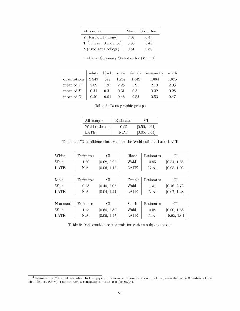
All sample Mean Std. Dev.
Y (log hourly wage) 2.08 0.47
T (college attendance) 0.30 0.46
Z (lived near college) 0.51 0.50
Table 2: Summary Statistics for (Y, T, Z)
white black male female non-south south
observations 2,249 329 1,267 1,642 1,884 1,025
mean of Y 2.09 1.97 2.28 1.91 2.10 2.03
mean of T 0.31 0.31 0.31 0.31 0.32 0.28
mean of Z 0.50 0.64 0.48 0.53 0.53 0.47
Table 3: Demographic groups
All sample Estimates CI
Wald estimand 0.95 [0.56, 1.61]
LATE N.A.4 [0.05, 1.04]
Table 4: 95% confidence intervals for the Wald estimand and LATE
White Estimates CI
Wald 1.20 [0.68, 2.25]
LATE N.A. [0.06, 1.16]
Male Estimates CI
Wald 0.93 [0.40, 2.07]
LATE N.A. [0.04, 1.44]
Non-south Estimates CI
Wald 1.15 [0.60, 2.30]
LATE N.A. [0.06, 1.47]
Black Estimates CI
Wald 0.95 [0.54, 1.66]
LATE N.A. [0.05, 1.06]
Female Estimates CI
Wald 1.31 [0.76, 2.72]
LATE N.A. [0.07, 1.28]
South Estimates CI
Wald 0.58 [0.00, 1.63]
LATE N.A. [-0.02, 1.04]
Table 5: 95% confidence intervals for various subpopulations
4Estimates for θ are not available. In this paper, I focus on an inference about the true parameter value θ, instead of theidentified set Θ0(P ). I do not have a consistent set estimator for Θ0(P ).
21

7 Identifying power of repeated measurements
This section explores the identifying power of repeated measurements. Repeated measurements (for example,
Hausman et al., 1991) is a popular approach in the literature on measurement error, but they cannot be
instrumental variables in this framework. This is because the true treatment variable T ∗ is endogenous and
it is natural to suspect that a measurement of T ∗ is also endogenous. The more accurate the measurement
is, the more likely it is to be endogenous. Nevertheless, the identification strategy of the present paper
incorporates repeated measurements as an additional information to narrow the identified set for LATE,
when they are coupled with the instrumental variable Z. Unlike the other paper on repeated measurements,
I do not need to assume the independence of measurement errors among multiple measurements. The
strategy of the present paper also benefits from having more than two measurements unlike Hausman et al.
(1991) who achieve the point identification with two measurements.
Consider a second measurement R for T ∗. I do not require that R is binary, so R can be discrete or
continuous. Like T = TT∗ , I model R using the counterfactual outcome notations. R1 is a counterfactual
second measurement when the true variable T ∗ is 1, and R0 is a counterfactual second measurement when
the true variable T ∗ is 0. Then the data generation of R is
R = RT∗ .
I assume that the instrumental variable Z is independent of Rt∗ conditional on (Yt∗ , Tt∗ , T∗z0 , T
∗z1).
Assumption 8. (i) Z is independent of (Rt∗ , Tt∗ , Yt∗ , T∗z0 , T
∗z1) for each t∗ = 0, 1. (ii) T ∗z1 ≥ T ∗z0 almost
surely.
Note that I do not assume the independence between Rt∗ and Tt∗ , where the independence between the
measurement errors is a key assumption when the repeated measurement is an instrumental variable.
Under this assumption, I refine the identified set for LATE as follows.
Theorem 4. Suppose that Assumption 8 holds, and consider an arbitrary data distribution P of (R, Y, T, Z).
(i) The sharp identified set ΘI(P ) for LATE is included in Θ0(P ), where Θ0(P ) is the set of θ’s which satisfies
the following three inequalities.
θ∆EP [Y | Z] ≥ 0
|θ| ≥ |∆EP [Y | Z]|
|θ|TV (f(R,Y,T )|Z=z1 , f(R,Y,T )|Z=z0) ≤ |∆EP [Y | Z]|.
(ii) If Y is unbounded, then ΘI(P ) is equal to Θ0(P ).
The total variation distance TV (f(R,Y,T )|Z=z1 , f(R,Y,T )|Z=z0) in Theorem 4 is weakly larger than that in
Theorem 1, which implies that the identified set in Theorem 4 is weakly smaller than the identified set in
22

Theorem 1:
TV (f(R,Y,T )|Z=z1 , f(R,Y,T )|Z=z0)
=1
2
∑t=0,1
∫∫|(f(R,Y,T )|Z=z1 − f(R,Y,T )|Z=z0)(r, y, t)|dµR(r)dµY (y)
≥ 1
2
∑t=0,1
∫|∫
(f(R,Y,T )|Z=z1 − f(R,Y,T )|Z=z0)(r, y, t)dµR(r)|dµY (y)
=1
2
∑t=0,1
∫|(f(Y,T )|Z=z1 − f(Y,T )|Z=z0)(y, t)|dµY (y)
= TV (f(Y,T )|Z=z1 , f(Y,T )|Z=z0)
and the strict inequality holds unless the sign of (f(R,Y,T )|Z=z1 − f(R,Y,T )|Z=z0)(r, y, t) is constant in r for
every (y, t). Therefore, it is possible to test whether the repeated measurement R has additional information,
by testing whether the sign of (f(R,Y,T )|Z=z1 − f(R,Y,T )|Z=z0)(r, y, t) is constant in r.
8 Conclusion
This paper studies the identifying power of instrumental variable in the heterogeneous treatment effect
framework when a binary treatment variable is mismeasured and endogenous. The assumptions in this
framework are the monotonicity of the instrumental variable Z on the true treatment variable T ∗ and the
exogeneity of Z. I use the total variation distance to characterize the identified set for LATE parameter
E[T1 − T0 | T ∗z0 < T ∗z1 ]. I also provide an inference procedure for LATE. Unlike the existing literature on
measurement error, the identification strategy does not reply on a specific assumption on the measurement
error; the only assumption on the measurement error is its independence of the instrumental variable. I
apply the new methodology to study the return to schooling in the proximity-to-college instrumental variable
regression using the NLS-72 dataset.
There are several directions for future research. First, the choice of the partition In in Section 4, par-
ticularly the choice of Kn, is an interesting direction. To the best of my knowledge, the literature on many
moment inequalities has not investigated how econometricians choose the numbers of the many moment in-
equalities. Second, it is worthwhile to investigating the other parameter for the treatment effect. This paper
has focused on the local average treatment effect (LATE) for the reasons mentioned in the introduction, but
the literature on heterogeneous treatment effect has emphasized the choice of treatment effect parameter as
an answer to relevant policy questions.
23

References
Aigner, D. J. (1973): “Regression with a Binary Independent Variable Subject to Errors of Observation,”Journal of Econometrics, 1, 49–59.
Amemiya, Y. (1985): “Instrumental Variable Estimator for the Nonlinear Errors-in-Variables Model,” Jour-nal of Econometrics, 28, 273–289.
Andrews, D. W. K. and P. J. Barwick (2012): “Inference for Parameters Defined by Moment Inequal-ities: A Recommended Moment Selection Procedure,” Econometrica, 80, 2805–2826.
Andrews, D. W. K. and P. Guggenberger (2009): “Hybrid and Size-Corrected Subsampling Methods,”Econometrica, 77, 721–762.
Andrews, D. W. K. and X. Shi (2013): “Inference Based on Conditional Moment Inequalities,” Econo-metrica, 81, 609–666.
Andrews, D. W. K. and G. Soares (2010): “Inference for Parameters Defined by Moment InequalitiesUsing Generalized Moment Selection,” Econometrica, 78, 119–157.
Angrist, J. D., G. W. Imbens, and D. B. Rubin (1996): “Identification of Causal Effects using Instru-mental Variables,” Journal of the American Statistical Association, 91, 444–455.
Angrist, J. D. and A. B. Krueger (1999): “Empirical Strategies in Labor Economics,” in Handbook ofLabor Economics, ed. by O. Ashenfelter and D. Card, Amsterdam: North Holland, vol. 3, 1277–1366.
——— (2001): “Instrumental Variables and the Search for Identification: From Supply and Demand toNatural Experiments,” Journal of Economic Perspectives, 15, 69–85.
Armstrong, T. B. (2014): “Weighted KS Statistics for Inference on Conditional Moment Inequalities,”Journal of Econometrics, 181, 92–116.
——— (2015): “Asymptotically Exact Inference in Conditional Moment Inequality Models,” Journal ofEconometrics, 186, 51–65.
Armstrong, T. B. and H. P. Chan (2014): “Multiscale Adaptive Inference on Conditional MomentInequalities,” Working paper.
Balke, A. and J. Pearl (1997): “Bounds on Treatment Effects from Studies with Imperfect Compliance,”Journal of the American Statistical Association, 92, 1171–1176.
Barron, J. M., M. C. Berger, and D. A. Black (1997): On-the-Job Training, Kalamazoo: WE UpjohnInstitute for Employment Research.
Besley, T. and S. Coate (1992): “Understanding Welfare Stigma: Taxpayer Resentment and StatisticalDiscrimination,” Journal of Public Economics, 48, 165–183.
Black, D., S. Sanders, and L. Taylor (2003): “Measurement of Higher Education in the Census andCurrent Population Survey,” Journal of the American Statistical Association, 98, 545–554.
Black, D. A., M. C. Berger, and F. A. Scott (2000): “Bounding Parameter Estimates with Nonclas-sical Measurement Error,” Journal of the American Statistical Association, 95, 739–748.
Blundell, R., A. Gosling, H. Ichimura, and C. Meghir (2007): “Changes in the Distribution of Maleand Female Wages Accounting for Employment Composition Using Bounds,” Econometrica, 75, 323–363.
Bollinger, C. R. (1996): “Bounding Mean Regressions When a Binary Regressor is Mismeasured,” Journalof Econometrics, 73, 387–399.
Bound, J., C. Brown, and N. Mathiowetz (2001): “Measurement Error in Survey Data,” in Handbookof Econometrics, ed. by J. Heckman and E. Leamer, Elsevier, vol. 5, chap. 59, 3705–3843.
24
Bugni, F. A. (2010): “Bootstrap Inference in Partially Identified Models Defined by Moment Inequalities:Coverage of the Identified Set,” Econometrica, 78, 735–753.
Canay, I. A. (2010): “EL Inference for Partially Identified Models: Large Deviations Optimality andBootstrap Validity,” Journal of Econometrics, 156, 408–425.
Card, D. (1995): “Using Geographic Variation in College Proximity to Estimate the Return to Schooling,”in Aspects of Labor Market Behaviour: Essays in Honour of John Vanderkamp, ed. by L. Christofides,E. Grant, and R. Swidinsky, Toronto: University of Toronto Press, 201–222.
——— (1999): “The Causal Effect of Education on Earnings,” in Handbook of Labor Economics, ed. byO. Ashenfelter and D. Card, Elsevier, vol. 3 of Handbook of Labor Economics, chap. 30, 1801–1863.
——— (2001): “Estimating the Return to Schooling: Progress on Some Persistent Econometric Problems,”Econometrica, 69, 1127–1160.
Carroll, R. J., D. Ruppert, L. A. Stefanski, and C. M. Crainiceanu (2012): Measurement Errorin Nonlinear Models: A Modern Perspective, Boca Raton: Chapman & Hall/CRC, 2nd ed.
Chalak, K. (2013): “Instrumental Variables Methods with Heterogeneity and Mismeasured Instruments,”Working paper.
Chernozhukov, V., D. Chetverikov, and K. Kato (2014): “Testing Many Moment Inequalities,”Working paper.
——— (2015): “Central Limit Theorems and Bootstrap in High Dimensions,” Working paper.
Chernozhukov, V., H. Hong, and E. Tamer (2007): “Estimation and Confidence Regions for ParameterSets in Econometric Models1,” Econometrica, 75, 1243–1284.
Chernozhukov, V., S. Lee, and A. M. Rosen (2013): “Intersection bounds: estimation and inference,”Econometrica, 81, 667–737.
Chetverikov, D. (2013): “Adaptive Test of Conditional Moment Inequalities,” Working paper.
de Chaisemartin, C. (2015): “Tolerating Defiance? Local Average Treatment Effects without Monotonic-ity,” Working paper.
Deaton, A. (2009): “Instruments of Development: Randomisation in the Tropics, and the Search for theElusive Keys to Economic Development: Keynes Lecture in Economics,” in Proceedings of the BritishAcademy, Volume 162, 2008 Lectures, Oxford: British Academy.
Fang, Z. and A. Santos (2014): “Inference on Directionally Differentiable Functions,” Working paper.
Frazis, H. and M. A. Loewenstein (2003): “Estimating Linear Regressions with Mismeasured, PossiblyEndogenous, Binary Explanatory Variables,” Journal of Econometrics, 117, 151–178.
Griliches, Z. (1977): “Estimating the Returns to Schooling: Some Econometric Problems,” Econometrica,45, 1–22.
Hausman, J. A., W. K. Newey, H. Ichimura, and J. L. Powell (1991): “Identification and Estimationof Polynomial Errors-in-Variables Models,” Journal of Econometrics, 50, 273–295.
Hausman, J. A., W. K. Newey, and J. L. Powell (1995): “Nonlinear Errors in Variables Estimationof Some Engel Curves,” Journal of Econometrics, 65, 205–233.
Heckman, J. J., D. Schmierer, and S. Urzua (2010): “Testing the Correlated Random CoefficientModel,” Journal of Econometrics, 158, 177–203.
Heckman, J. J. and S. Urzua (2010): “Comparing IV with Structural Models: What Simple IV Can andCannot Identify,” Journal of Econometrics, 156, 27–37.
25

Heckman, J. J. and E. Vytlacil (2005): “Structural Equations, Treatment Effects, and EconometricPolicy Evaluation,” Econometrica, 73, 669–738.
Henry, M., K. Jochmans, and B. Salanie (2015): “Inference on Two-Component Mixtures under TailRestrictions,” Econometric Theory, forthcoming.
Henry, M., Y. Kitamura, and B. Salanie (2014): “Partial Identification of Finite Mixtures in Econo-metric Models,” Quantitative Economics, 5, 123–144.
Hernandez, M. and S. Pudney (2007): “Measurement Error in Models of Welfare Participation,” Journalof Public Economics, 91, 327–341.
Hirano, K. and J. R. Porter (2012): “Impossibility Results for Nondifferentiable Functionals,” Econo-metrica, 80, 1769–1790.
Hsiao, C. (1989): “Consistent Estimation for Some Nonlinear Errors-in-Variables Models,” Journal ofEconometrics, 41, 159–185.
Hu, Y. (2008): “Identification and Estimation of Nonlinear Models with Misclassification Error using In-strumental Variables: A General Solution,” Journal of Econometrics, 144, 27–61.
Hu, Y., J.-L. Shiu, and T. Woutersen (2015): “Identification and Estimation of Single Index Modelswith Measurement Error and Endogeneity,” Econometrics Journal, forthcoming.
Huber, M. and G. Mellace (2015): “Testing Instrument Validity for LATE Identification Based onInequality Moment Constraints,” Review of Economics and Statistics, 97, 398–411.
Imai, K. and T. Yamamoto (2010): “Causal Inference with Differential Measurement Error: Nonpara-metric Identification and Sensitivity Analysis,” American Journal of Political Science, 54, 543–560.
Imbens, G. W. (2010): “Better LATE Than Nothing: Some Comments on Deaton (2009) and Heckmanand Urzua (2009),” Journal of Economic Literature, 48, 399–423.
——— (2014): “Instrumental Variables: An Econometrician’s Perspective,” Statistical Science, 29, 323–358.
Imbens, G. W. and J. D. Angrist (1994): “Identification and Estimation of Local Average TreatmentEffects,” Econometrica, 62, 467–75.
Imbens, G. W. and C. F. Manski (2004): “Confidence Intervals for Partially Identified Parameters,”Econometrica, 72, 1845–1857.
Kaestner, R., T. Joyce, and H. Wehbeh (1996): “The Effect of Maternal Drug Use on Birth Weight:Measurement Error in Binary Variables,” Economic Inquiry, 34, 617–629.
Kane, T. J. and C. E. Rouse (1995): “Labor-Market Returns to Two- and Four-Year College,” AmericanEconomic Review, 85, 600–614.
Kane, T. J., C. E. Rouse, and D. Staiger (1999): “Estimating Returns to Schooling When Schoolingis Misreported,” NBER Working Paper No. 7235.
Kim, K. I. (2009): “Set Estimation and Inference with Models Characterized by Conditional MomentInequalities,” Working paper.
Kitagawa, T. (2010): “Testing for Instrument Independence in the Selection Model,” Working paper.
——— (2014): “A Test for Instrument Validity,” Econometrica, forthcoming.
Kreider, B. and J. V. Pepper (2007): “Disability and Employment: Reevaluating the Evidence in Lightof Reporting Errors,” Journal of the American Statistical Association, 102, 432–441.
26

Kreider, B., J. V. Pepper, C. Gundersen, and D. Jolliffe (2012): “Identifying the Effects of SNAP(Food Stamps) on Child Health Outcomes when Participation is Endogenous and Misreported,” Journalof the American Statistical Association, 107, 958–975.
Lewbel, A. (1998): “Semiparametric Latent Variable Model Estimation with Endogenous or MismeasuredRegressors,” Econometrica, 66, 105–121.
——— (2007): “Estimation of Average Treatment Effects with Misclassification,” Econometrica, 75, 537–551.
Mahajan, A. (2006): “Identification and Estimation of Regression Models with Misclassification,” Econo-metrica, 74, 631–665.
Manski, C. F. (2003): Partial Identification of Probability Distributions, New York: Springer-Verlag.
Menzel, K. (2014): “Consistent Estimation with Many Moment Inequalities,” Journal of Econometrics,182, 329–350.
Moffitt, R. (1983): “An Economic Model of Welfare Stigma,” American Economic Review, 73, 1023–1035.
Molinari, F. (2008): “Partial Identification of Probability Distributions with Misclassified Data,” Journalof Econometrics, 144, 81–117.
Mourifie, I. Y. and Y. Wan (2014): “Testing Local Average Treatment Effect Assumptions,” Workingpaper.
Ponomareva, M. (2010): “Inference in Models Defined by Conditional Moment Inequalities with Contin-uous Covariates,” Working paper.
Romano, J. P. and A. M. Shaikh (2008): “Inference for identifiable parameters in partially identifiedeconometric models,” Journal of Statistical Planning and Inference, 138, 2786–2807.
——— (2010): “Inference for the Identified Set in Partially Identified Econometric Models,” Econometrica,78, 169–211.
Rosen, A. M. (2008): “Confidence Sets for Partially Identified Parameters That Satisfy a Finite Numberof Moment Inequalities,” Journal of Econometrics, 146, 107–117.
Royalty, A. B. (1996): “The Effects of Job Turnover on the Training of Men and Women,” Industrial &Labor Relations Review, 49, 506–521.
Schennach, S. M. (2013): “Measurement Error in Nonlinear Models - A Review,” in Advances in Eco-nomics and Econometrics: Economic theory, ed. by D. Acemoglu, M. Arellano, and E. Dekel, CambridgeUniversity Press, vol. 3, 296–337.
Song, S. (2015): “Semiparametric Estimation of Models with Conditional Moment Restrictions in thePresence of Nonclassical Measurement Errors,” Journal of Econometrics, 185, 95–109.
Song, S., S. M. Schennach, and H. White (2015): “Estimating Nonseparable Models with MismeasuredEndogenous Variables,” Quantitative Economics, forthcoming.
Stoye, J. (2009): “More on Confidence Intervals for Partially Identified Parameters,” Econometrica, 77,1299–1315.
27

A Proofs of Lemmas 1, 2, and 3
Proof of Lemma 1. Eq. (4) implies
θ(P ∗)∆EP∗ [Y | Z] = θ(P ∗)2P ∗(T ∗z0 < T ∗z1)
≥ 0
and
|∆EP∗ [Y | Z]| = |θ(P ∗)P ∗(T ∗z0 < T ∗z1)|
≤ |θ(P ∗)|,
because 0 ≤ P ∗(T ∗z0 < T ∗z1) ≥ 1.
Proof of Lemma 2. I obtain
f(Y,T )|Z=z1 − f(Y,T )|Z=z0 = P ∗(T ∗z0 < T ∗z1)(f(Y1,T1)|T∗z0<T∗z1− f(Y0,T0)|T∗z0<T
∗z1
)
by applying the same logic as Theorem 1 in Imbens and Angrist (1994):
f(Y,T )|Z=z0 = P ∗(T ∗z0 = T ∗z1 = 1 | Z = z0)f(Y,T )|Z=z0,T∗z0=T∗z1
=1
+P ∗(T ∗z0 < T ∗z1 | Z = z0)f(Y,T )|Z=z0,T∗z0<T∗z1
+P ∗(T ∗z0 = T ∗z1 = 0 | Z = z0)f(Y,T )|Z=z0,T∗z0=T∗z1
=0
= P ∗(T ∗z0 = T ∗z1 = 1)f(Y1,T1)|T∗z0=T∗z1=1
+P ∗(T ∗z0 < T ∗z1)f(Y0,T0)|T∗z0<T∗z1
+P ∗(T ∗z0 = T ∗z1 = 0)f(Y0,T0)|T∗z0=T∗z1=0
f(Y,T )|Z=z1 = P ∗(T ∗z0 = T ∗z1 = 1)f(Y1,T1)|T∗z0=T∗z1=1
+P ∗(T ∗z0 < T ∗z1)f(Y1,T1)|T∗z0<T∗z1
+P ∗(T ∗z0 = T ∗z1 = 0)f(Y0,T0)|T∗z0=T∗z1=0.
This implies
TV (f(Y,T )|Z=z1 , f(Y,T )|Z=z0)
=1
2
∑t=0,1
∫|f(Y,T )|Z=z1(y, t)− f(Y,T )|Z=z0(y, t)|dµY (y)
=1
2
∑t=0,1
∫|P ∗(T ∗z0 < T ∗z1)(f(Y1,T1)|T∗z0<T
∗z1
(y, t)− f(Y0,T0)|T∗z0<T∗z1
(y, t))|dµY (y)
= P ∗(T ∗z0 < T ∗z1)1
2
∑t=0,1
∫|(f(Y1,T1)|T∗z0<T
∗z1
(y, t)− f(Y0,T0)|T∗z0<T∗z1
(y, t))|dµY (y)
= P ∗(T ∗z0 < T ∗z1)TV (f(Y1,T1)|T∗z0<T∗z1, f(Y0,T0)|T∗z0<T
∗z1
)
≤ P ∗(T ∗z0 < T ∗z1),
where the last inequality follows because the total variation distance is at most one. Moreover, since T ∗z0 ≤ T∗z1
28

almost surely,
P ∗(T ∗z0 < T ∗z1), = |P ∗(T ∗z0 = 1)− P ∗(T ∗z1 = 1)|
=1
2|P ∗(T ∗z0 = 1)− P ∗(T ∗z1 = 1)|+ 1
2|P ∗(T ∗z0 = 0)− P ∗(T ∗z1 = 0)|
=1
2
∑t∗=0,1
|fT∗|Z=z1(t∗)− fT∗|Z=z0(t∗)|
= TV (fT∗|Z=z1 , fT∗|Z=z0).
Proof of Lemma 3. The lemma follows from
∆EP [h(Y, T ) | Z] = EP [h(Y, T ) | Z = z1]− EP [h(Y, T ) | Z = z0]
=∑t=0,1
∫h(y, t)(f(Y,T )|Z=z1(y, t)− f(Y,T )|Z=z0(y, t))dµY (y)
=∑t=0,1
∫h(y, t)∆f(Y,T )|Z(y, t)dµY (y)
≤∑t=0,1
∫|∆f(Y,T )|Z(y, t)|dµY (y)
= 2× TV (f(Y,T )|Z=z1 , f(Y,T )|Z=z0)
where the maximization is achieved if h(y, t) = 1 if ∆f(Y,T )|Z(y, t) > 0 and h(y, t) = −1 if ∆f(Y,T )|Z(y, t) <
0.
B Proofs of Theorems 1 and 4
Theorem 1 is a special case of Theorem 4 with R being constant, and therefore I demonstrate the proof only
for Theorem 4. Lemma 2 is modified into the following lemma in the framework of Theorem 4.
Lemma 4. Under Assumption 8, then
TV (f(R,Y,T )|Z=z1 , f(R,Y,T )|Z=z0) ≤ P ∗(T ∗z0 < T ∗z1).
Proof. The proof is the same as Lemma 2 and this lemma follows from
f(R,Y,T )|Z=z1 − f(R,Y,T )|Z=z0 = P ∗(T ∗z0 < T ∗z1)(f(R1,Y1,T1)|T∗z0<T∗z1− f(R0,Y0,T0)|T∗z0<T
∗z1
).
From Lemmas 1 and 4, all the three inequalities in Theorem 4 are satisfied when θ is the true value
for LATE, which is the first part of Theorem 4. To prove Theorem 4, I am going to show the sharpness
of the three inequalities, that is, that any point satisfying the three inequalities is generated by some data
generating process P ∗ which is consistent with the data distribution P . I will consider two cases based on
the value of TV (f(R,Y,T )|Z=z1 , f(R,Y,T )|Z=z0).
29

B.1 Case 1: Zero total variation distance
Consider TV (f(R,Y,T )|Z=z1 , f(R,Y,T )|Z=z0) = 0. In this case, f(R,Y,T )|Z=z1 = f(R,Y,T )|Z=z0 almost everywhere
over (r, y, t) and particularly ∆EP [Y | Z] = 0. Note that all the three inequalities in Theorem 4 have no
restriction on θ in this case. For every y ∈ R, consider the following two data generating processes. First,
P ∗y,L is defined by
Z ∼ P (Z = z)
(T ∗z0 , T∗z1) | Z =
(0, 1) with probability P (Y > y)
(1, 1) with probability P (Y ≤ y)
(R1, Y1, T1) | (T ∗z0 , T∗z1 , Z) ∼ f(R,Y,T )(r, y, t)
(R0, Y0, T0) | (T ∗z0 , T∗z1 , Z) ∼
f(R,Y,T )|Y >y(r, y, t) if T ∗z0 < T ∗z1
f(R,Y,T )|Y≤y(r, y, t) if T ∗z0 = T ∗z1
where (R1, Y1, T1) and (R0, Y0, T0) are conditionally independent of (T ∗z0 , T∗z1 , Z). Second, P ∗y,U is defined by
Z ∼ P (Z = z)
(T ∗z0 , T∗z1) | Z =
(0, 1) with probability P (Y < y)
(1, 1) with probability P (Y ≥ y)
(R1, Y1, T1) | (T ∗z0 , T∗z1 , Z) ∼ f(R,Y,T )(r, y, t)
(R0, Y0, T0) | (T ∗z0 , T∗z1 , Z) ∼
f(R,Y,T )|Y <y(r, y, t) if T ∗z0 < T ∗z1
f(R,Y,T )|Y≥y(r, y, t) if T ∗z0 = T ∗z1
where (R1, Y1, T1) and (R0, Y0, T0) are conditionally independent of (T ∗z0 , T∗z1 , Z).
Lemma 5. Consider the assumptions in Theorem 4. If TV (f(R,Y,T )|Z=z1 , f(R,Y,T )|Z=z0) = 0, then, for every
y ∈ R and every π ∈ [0, 1],
1. the mixture distribution πP ∗y,L + (1− π)P ∗y,U satisfies Assumption 8;
2. the mixture distribution πP ∗y,L + (1− π)P ∗y,U generates the data distribution P ;
3. under the mixture distribution πP ∗y,L + (1− π)P ∗y,U , LATE is equal to EP [Y ]− πEP [Y | Y > y]− (1−π)EP [Y | Y < y].
Proof. (1) Both P ∗y,L and P ∗y,U satisfy the independence between Z and (Rt∗ , Tt∗ , Yt∗ , T∗z0 , T
∗z1) for each
t∗ = 0, 1. Furthermore, P ∗y,L and P ∗y,U have the same marginal distribution for Z: P (Z = z). Therefore,
the mixture of P ∗y,L and P ∗y,U also satisfies the independence. Since the mixture of P ∗y,L and P ∗y,U satisfies
T ∗z1 ≥ T∗z0 almost surely, the first part of this lemma is established.
(2) The second part follows from the fact that both P ∗y,L and P ∗y,U generate the data distribution P .
Since the proof is essentially the same for P ∗y,L and P ∗y,U , I demonstrate it only for P ∗y,L. Denote by f∗ the
30

density function of P ∗y,L. Then
f∗(R,Y,T )|Z=z0(r, y, t) = P ∗y,L(T ∗z0 < T ∗z1)f∗(R,Y,T )|T∗z0<T
∗z1,Z=z0
(r, y, t)
+P ∗y,L(T ∗z0 = T ∗z1 = 1)f∗(R,Y,T )|T∗z0=T∗z1=1,Z=z0
(r, y, t)
= P ∗y,L(T ∗z0 < T ∗z1)f∗(R0,Y0,T0)|T∗z0<T∗z1
(r, y, t)
+P ∗y,L(T ∗z0 = T ∗z1 = 1)f∗(R1,Y1,T1)|T∗z0=T∗z1=1(r, y, t)
= P (Y > y)f(R,Y,T )|Y >y(r, y, t)
+P (Y ≤ y)f(R,Y,T )|Y≤y(r, y, t)
= f(R,Y,T )(r, y, t)
f∗(R,Y,T )|Z=z1(r, y, t) = f(R,Y,T )(r, y, t),
where the last equality uses Z = z1 implies T ∗ = 1.
(3) LATE under P ∗y,L is
EP∗y,L[Y1 − Y0 | T ∗z0 < T ∗z1 ] = EP∗y,L
[Y1 | T ∗z0 < T ∗z1 ]− EP∗y,L[Y0 | T ∗z0 < T ∗z1 ]
= EP [Y ]− EP [Y | Y > y]
and LATE under P ∗y,U is
EP∗y,L[Y1 − Y0 | T ∗z0 < T ∗z1 ] = EP∗y,L
[Y1 | T ∗z0 < T ∗z1 ]− EP∗y,L[Y0 | T ∗z0 < T ∗z1 ]
= EP [Y ]− EP [Y | Y < y].
They imply that LATE under the mixture distribution is equal to EP [Y ]− πEP [Y | Y > y]− (1− π)EP [Y |Y < y].
Now I will prove Theorem 4 for Case 1. Let θ be any real number. Since Y is unbounded, there are yL
and yU with yL ≤ EP [Y ]− θ ≤ yU such that P (Y < yL) > 0 and P (Y > yL) > 0. Since
EP [Y | Y < yL] ≤ EP [Y ]− θ ≤ EP [Y | Y > yU ],
there is π ∈ [0, 1] such that
θ = EP [Y ]− πEP [Y | Y > yU ]− (1− π)EP [Y | Y < yL].
Using Lemma 5, the right hand side of the above equation is LATE under the mixture distribution πP ∗yL,L+
(1− π)P ∗yU ,U . This proves that θ is LATE under some data generating process which is consistent with the
observed distribution P .
31

B.2 Case 2: Positive total variation distance
Consider TV (f(R,Y,T )|Z=z1 , f(R,Y,T )|Z=z0) > 0. This means that the instrumental variable Z has non-zero
indirect effect on (R, Y, T ). Consider the following two data generating processes. First, P ∗L is defined by
Z ∼ P (Z = z)
(T ∗z0 , T∗z1) | Z = (0, 1)
(R0, Y0, T0) | (T ∗z0 , T∗z1 , Z) ∼ f(R,Y,T )|Z=z0
(R1, Y1, T1) | (T ∗z0 , T∗z1 , Z) ∼ f(R,Y,T )|Z=z1
where (R1, Y1, T1) and (R0, Y0, T0) are conditionally independent of (T ∗z0 , T∗z1 , Z). Second, P ∗U defined as
follows. Define
H = 1∆f(R,Y,T )|Z(R, Y, T ) ≥ 0 − 1∆f(R,Y,T )|Z(R, Y, T ) < 0.
and define P ∗U as
Z ∼ P (Z = z)
(T ∗z0 , T∗z1) | Z =
(0, 1) with probability ∆EP [H | Z]/2
(0, 0) with probability P (H = −1 | Z = z1)
(1, 1) with probability P (H = 1 | Z = z0)
(R1, Y1, T1) | (T ∗z0 , T∗z1 , Z) ∼
∆f(R,Y,T,H)|Z(r,y,t,1)
∆EP [H|Z]/2 if T ∗z0 < T ∗z1
any distribution if T ∗z0 = T ∗z1 = 0
f(R,Y,T )|H=1,Z=z0(r, y, t) if T ∗z0 = T ∗z1 = 1
(R0, Y0, T0) | (T ∗z0 , T∗z1 , Z) ∼
−∆f(R,Y,T,H)|Z(r,y,t,−1)
∆EP [H|Z]/2 if T ∗z0 < T ∗z1
f(R,Y,T )|H=0,Z=z1(y, t) if T ∗z0 = T ∗z1 = 0
any distribution if T ∗z0 = T ∗z1 = 1
where (R1, Y1, T1) and (R0, Y0, T0) are conditionally independent of (T ∗z0 , T∗z1 , Z).
Lemma 6. Consider the assumptions in Theorem 4. If TV (f(R,Y,T )|Z=z1 , f(R,Y,T )|Z=z0) > 0, then
1. P ∗L generates the data distribution P and LATE under P ∗L is equal to ∆EP [Y | Z]; and
2. P ∗U generates the data distribution P and LATE under P ∗U is equal to
∆EP [Y | Z]/TV (f(R,Y,T )|Z=z1 , f(R,Y,T )|Z=z0).
32

Proof. (1) Denote by f∗ the density function of P ∗L. P ∗L generates the data distribution P :
f∗(R,Y,T )|Z=z0(r, y, t) = f∗(R,Y,T )|T∗=0,Z=z0
(r, y, t)
= f∗(R0,Y0,T0)|T∗=0,Z=z0(r, y, t)
= f(R,Y,T )|Z=z0(r, y, t)
f∗(R,Y,T )|Z=z1(r, y, t) = f∗(R,Y,T )|T∗=1,Z=z1
(r, y, t)
= f∗(R1,Y1,T1)|T∗=1,Z=z1(r, y, t)
= f(R,Y,T )|Z=z1(r, y, t)
where the first equality uses T ∗ = 1Z = z1. Under P ∗L, LATE is equal to ∆EP [Y | Z]:
EP∗L [Y1 − Y0 | T ∗z0 < T ∗z1 ] = EP∗L [Y1]− EP∗L [Y0]
= EP [Y | Z = z1]− EP [Y | Z = z0]
= ∆EP [Y | Z].
(2) Denote by f∗ the density function of P ∗U . When ∆EP [Y | Z] 6= 0, f∗(Rt∗ ,Yt∗ ,Tt∗ )|(T∗z0 ,T∗z1
) is positive on
:
∆f(R,Y,T,H)|Z(r, y, t, 1) = ∆f(R,Y,T )|Z(r, y, t)1∆f(R,Y,T )|Z(r, y, t) ≥ 0
≥ 0
∆f(R,Y,T,H)|Z(r, y, t,−1) = ∆f(R,Y,T )|Z(r, y, t)1∆f(R,Y,T )|Z(r, y, t) < 0
< 0.
P ∗U generates the data distribution P :
f∗(R,Y,T )|Z=z0(r, y, t) = P ∗U (T ∗z0 < T ∗z1 | Z = z0)f∗(R,Y,T )|T∗z0<T
∗z1,Z=z0
(r, y, t)
+P ∗U (T ∗z1 = T ∗z0 = 0 | Z = z0)f∗(R,Y,T )|T∗z1=T∗z0=0,Z=z0(r, y, t)
+P ∗U (T ∗z1 = T ∗z0 = 1 | Z = z0)f∗(R,Y,T )|T∗z1=T∗z0=1,Z=z0
(r, y, t)
= P ∗U (T ∗z0 < T ∗z1)f∗(R0,Y0,T0)|T∗z0<T∗z1
(r, y, t)
+P ∗U (T ∗z1 = T ∗z0 = 0)f∗(R0,Y0,T0)|T∗z1=T∗z0=0(r, y, t)
+P ∗U (T ∗z1 = T ∗z0 = 1)f∗(R1,Y1,T1)|T∗z1=T∗z0=1(r, y, t)
= −∆EP [H | Z]
2
∆f(R,Y,T,H)|Z(r, y, t,−1)
∆EP [H | Z]/2
+P (H = −1 | Z = z1)f(R,Y,T )|H=−1,Z=z1(r, y, t)
+P (H = 1 | Z = z0)f(R,Y,T )|H=1,Z=z0(r, y, t)
= f(R,Y,T )|Z=z0(r, y, t).
33

f∗(R,Y,T )|Z=z1(r, y, t) = P ∗U (T ∗z0 < T ∗z1 | Z = z1)f∗(R,Y,T )|T∗z0<T
∗z1,Z=z1
(r, y, t)
+P ∗U (T ∗z1 = T ∗z0 = 0 | Z = z1)f∗(R,Y,T )|T∗z1=T∗z0=0,Z=z1
(r, y, t)
+P ∗U (T ∗z1 = T ∗z0 = 1 | Z = z1)f∗(R,Y,T )|T∗z1=T∗z0=1,Z=z1
(r, y, t)
= P ∗U (T ∗z0 < T ∗z1)f∗(R1,Y1,T1)|T∗z0<T∗z1
(r, y, t)
+P ∗U (T ∗z1 = T ∗z0 = 0)f∗(R0,Y0,T0)|T∗z1=T∗z0=0(r, y, t)
+P ∗U (T ∗z1 = T ∗z0 = 1)f∗(R1,Y1,T1)|T∗z1=T∗z0=1(r, y, t)
= ∆EP [H | Z]/2∆f(R,Y,T,H)|Z(r, y, t, 1)
∆EP [H | Z]/2
+P (H = −1 | Z = z1)f(R,Y,T )|H=−1,Z=z1(r, y, t)
+P (H = 1 | Z = z0)f(R,Y,T )|H=1,Z=z0(r, y, t)
= f(R,Y,T )|Z=z1(r, y, t).
Under P ∗U , LATE is equal to ∆EP [Y | Z]/TV (f(R,Y,T )|Z=z1 , f(R,Y,T )|Z=z0):
∆EP∗U [H | Z]/2
=1
2
∑t=0,1
∫∫(1∆f(R,Y,T )|Z(r, y, t) ≥ 0 − 1∆f(R,Y,T )|Z(r, y, t) < 0)∆f(R,Y,T )|Z(r, y, t)dµY (y)dµR(r)
=1
2
∑t=0,1
∫∫|∆f(R,Y,T )|Z(r, y, t)|dµY (y)dµR(r)
= TV (f(R,Y,T )|Z=z1 , f(R,Y,T )|Z=z0)
EP∗U [Y1 − Y0 | T ∗z0 < T ∗z1 ] =∑t=0,1
∫∫y
(∆f(R,Y,T,H)|Z(r, y, t, 1)
∆EP [H | Z]/2+
∆f(R,Y,T,H)(y, t,−1)
∆EP [H | Z]/2
)dµY (y)dµR(r)
=∑t=0,1
∫∫y
∆f(R,Y,T )|Z(r, y, t)
∆EP [H | Z]/2dµY (y)dµR(r)
=∆EP [Y | Z]
∆EP [H | Z]/2
=∆EP [Y | Z]
TV (f(R,Y,T )|Z=z1 , f(R,Y,T )|Z=z0).
Lemma 7. Consider the assumptions in Theorem 4. If TV (f(R,Y,T )|Z=z1 , f(R,Y,T )|Z=z0) > 0, then, for every
π ∈ [0, 1],
1. the mixture distribution πP ∗L + (1− π)P ∗U satisfies Assumption 1;
2. the mixture distribution πP ∗L + (1− π)P ∗U generates the data distribution P ;
3. under the mixture distribution πP ∗L + (1− π)P ∗U , LATE is equal to
π∆EP [Y | Z] + (1− π)∆EP [Y | Z]
TV (f(R,Y,T )|Z=z1 , f(R,Y,T )|Z=z0).
Proof. The proof for this lemma is the same as the proof in Lemma 4.
34

Now I will prove Theorem 4 for Case 2. Let θ be any real number satisfying all the three inequalities in
Theorem 4. Then there is π ∈ [0, 1] such that
θ = π∆EP [Y | Z] + (1− π)∆EP [Y | Z]
TV (f(R,Y,T )|Z=z1 , f(R,Y,T )|Z=z0).
Using Lemma 7, the right hand side of the above equation is LATE under the mixture distribution πP ∗L +
(1 − π)P ∗U . This proves that θ is LATE under some data generating process which is consistent with the
observed distribution P .
C Proofs of Theorems 2 and 3
These results are obtained by applying the results in Chernozhukov et al. (2014) for two independent samples.
I use the same notation as them and modify their proofs to the two samples. First, I introduce the following
lemma.
Lemma 8. (1) If x1, x2 are p-dimensional random variables and 0 < x2,j ≤ 1, then∣∣∣∣ max1≤j≤p
x1,jx2,j
∣∣∣∣ ≤ ∣∣∣∣ max1≤j≤p
x1,j
∣∣∣∣ .(2) If X1, X1, X2, X2 are p-dimensional random variables and if (X1, X1) and (X2, X2) are independent,
then
supt∈Rp
|P (X1 +X2 ≤ t)− P (X1 + X2 ≤ t)| ≤ supt∈Rp
|P (X1 ≤ t)− P (X1 ≤ t)|
+ supt∈Rp
|P (X2 ≤ t)− P (X2 ≤ t)|.
(3) If x1, x2 are p-dimensional random variables and x2,j > 0, then
| max1≤j≤p
x1,j − max1≤j≤p
x1,jx2,j | ≤∣∣∣∣ max1≤j≤p
x1,j
∣∣∣∣ max1≤j≤p
|x2,j − 1| .
Proof. The first statement is as follows. If max1≤j≤p x1,j ≥ 0, then∣∣∣∣ max1≤j≤p
x1,jx2,j
∣∣∣∣ = max1≤j≤p
x1,j1x1,j > 0x2,j ≤ max1≤j≤p
x1,j1x1,j > 0 = max1≤j≤p
x1,j .
If max1≤j≤p x1,j < 0, then∣∣∣∣ max1≤j≤p
x1,jx2,j
∣∣∣∣ = min1≤j≤p
(−x1,j)x2,j ≤ min1≤j≤p
(−x1,j) = − max1≤j≤p
x1,j .
35

The second statement is as follows.
supt∈Rp
|P (X1 +X2 ≤ t)− P (X1 + X2 ≤ t)|
≤ supt∈Rp
|P (X1 +X2 ≤ t)− P (X1 +X2 ≤ t)|
+ supt∈Rp
|P (X1 +X2 ≤ t)− P (X1 + X2 ≤ t)|
= supt∈Rp
|E[P (X1 +X2 ≤ t | X2)− P (X1 +X2 ≤ t | X2)]|
+ supt∈Rp
|E[P (X1 +X2 ≤ t | X1)− P (X1 + X2 ≤ t | X1)]|
≤ supt∈Rp
|P (X1 ≤ t)− P (X1 ≤ t)|
+ supt∈Rp
|P (X2 ≤ t)− P (X2 ≤ t)|.
The third statement is as follows. If max1≤j≤p x1,jx2,j ≥ max1≤j≤p x1,j ≥ 0, then∣∣∣∣ max1≤j≤p
x1,j − max1≤j≤p
x1,jx2,j
∣∣∣∣ =
∣∣∣∣ max1≤j≤p
x1,j
∣∣∣∣ ( max1≤j≤p
x1,j1x1,j > 0max1≤j≤p x1,j1x1,j > 0
x2,j − 1
)≤
∣∣∣∣ max1≤j≤p
x1,j
∣∣∣∣ ( max1≤j≤p
x2,j − 1
).
If 0 > max1≤j≤p x1,jx2,j ≥ max1≤j≤p x1,j , then∣∣∣∣ max1≤j≤p
x1,j − max1≤j≤p
x1,jx2,j
∣∣∣∣ =
∣∣∣∣ max1≤j≤p
x1,j
∣∣∣∣ (1− min1≤j≤p
(−x1,j)
min1≤j≤p(−x1,j)x2,j
)≤
∣∣∣∣ max1≤j≤p
x1,j
∣∣∣∣ (1− min1≤j≤p
x2,j
).
If max1≤j≤p x1,j ≥ max1≤j≤p x1,jx2,j ≥ 0, then∣∣∣∣ max1≤j≤p
x1,j − max1≤j≤p
x1,jx2,j
∣∣∣∣ =
∣∣∣∣ max1≤j≤p
x1,j
∣∣∣∣ (1− max1≤j≤p x1,j1x1,j > 0x2,j
max1≤j≤p x1,j1x1,j > 0
)≤
∣∣∣∣ max1≤j≤p
x1,j
∣∣∣∣ (1− max1≤j≤p x1,j1x1,j > 0min1≤j≤p x2,j
max1≤j≤p x1,j1x1,j > 0
)=
∣∣∣∣ max1≤j≤p
x1,j
∣∣∣∣ (1− min1≤j≤p
x2,j
).
If 0 > max1≤j≤p x1,j ≥ max1≤j≤p x1,jx2,j , then∣∣∣∣ max1≤j≤p
x1,j − max1≤j≤p
x1,jx2,j
∣∣∣∣ =
∣∣∣∣ max1≤j≤p
x1,j
∣∣∣∣ (max1≤j≤p(−x1,j)x2,j
max1≤j≤p(−x1,j)− 1
)≤
∣∣∣∣ max1≤j≤p
x1,j
∣∣∣∣ (max1≤j≤p(−x1,j) max1≤j≤p x2,j
max1≤j≤p(−x1,j)− 1
)=
∣∣∣∣ max1≤j≤p
x1,j
∣∣∣∣ ( max1≤j≤p
x2,j − 1
).
Now I modify Chernozhukov et al. (2014) for two independent sample. In order to simplify the notations,
this section focuses on a fixed value of θ and omits θ in the following discussion. All the following results are
36
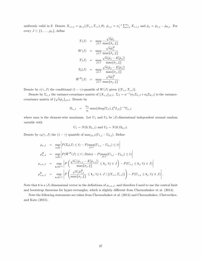
uniformly valid in θ. Denote Xz,i,j = gz,j((Yz,i, Tz,i), θ), µz,j = n−1z
∑nz
i=1Xz,i,j and µj = µ1,j − µ0,j . For
every J ⊂ 1, . . . , pn, define
T (J) = maxj∈J
√nµj
maxσj , ξ
W (J) = maxj∈J
√nµBj
maxσj , ξ
T (J) = maxj∈J
√n(µj − E[µj ])
maxσj , ξ
T0(J) = maxj∈J
√n(µj − E[µj ])
maxσj , ξ
WB(J) = maxj∈J
√nµBj
maxσj , ξ.
Denote by c(γ, J) the conditional (1− γ)-quantile of W (J) given (Yz,i, Tz,i).Denote by Σz,J the variance-covariance matrix of Xz,jj∈J . ΣJ = n−1(n1Σ1,J +n0Σ0,J) is the variance-
covariance matrix of √nµjj∈J . Denote by
Ωz,J =nzn
maxdiag(ΣJ), ξ2I|J|−1Σz,J
where max is the element-wise maximum. Let U1 and U0 be |J |-dimensional independent normal random
variable with
U1 ∼ N(0,Ω1,J) and U0 ∼ N(0,Ω0,J).
Denote by c0(γ, J) the (1− γ) quantile of maxj∈J(U1,j − U0,j). Define
ρn,J = supt∈R
∣∣∣∣P (T0(J) ≤ t)− P (maxj∈J
(U1,j − U0,j) ≤ t)∣∣∣∣
ρBn,J = supt∈R
∣∣∣∣P (WB(J) ≤ t | Data)− P (maxj∈J
(U1,j − U0,j) ≤ t)∣∣∣∣
ρz,n,J = supt∈R|J|
∣∣∣∣P (√nz(µz,j − E[µz,j ])
maxσj , ξ≤ tj ,∀j ∈ J
)− P (Uz,j ≤ tj ,∀j ∈ J)
∣∣∣∣ρBz,n,J = sup
t∈R|J|
∣∣∣∣∣P( √
nzµBz,j
maxσj , ξ≤ tj ,∀j ∈ J | (Yz,i, Tz,i)
)− P (Uz,j ≤ tj ,∀j ∈ J)
∣∣∣∣∣ .Note that t is a |J |-dimensional vector in the definitions of ρz,n,J , and therefore I need to use the central limit
and bootstrap theorems for hyper-rectangles, which is slightly different from Chernozhukov et al. (2014).
Note the following statements are taken from Chernozhukov et al. (2014) and Chernozhukov, Chetverikov,
and Kato (2015).
37

Lemma 9. (1) There are positive numbers c ∈ (0, 1/2) and C > 0 such that
ρz,n,J ≤ Cn−cz (8)
P (ρBz,n,J < Cνz,n) ≥ 1− Cn−cz with some νz,n = Cn−cz (9)
P
(maxj∈J
∣∣∣∣∣σ2z,j
σ2z,j
− 1
∣∣∣∣∣ > n−1/2+c1/4z B2
z,nzlog(|J |)
)≤ Cn−cz (10)
P
(maxj∈J
∣∣∣∣√nz(µz,j − E[µz,j ])
σz,j
∣∣∣∣ > nc1/4z
√log(|J |)
)≤ Cn−cz . (11)
(2) The following inequalities hold:
EP
[∣∣∣∣∣maxj∈J
√nzµ
Bz,j
σz,j
∣∣∣∣∣ | Data]≤√
2 log(2|J |) (12)
c0(γ, J) ≤√
2 log(|J |) +√
2 log(1/γ) (13)
P
(∣∣∣∣maxj∈J
(U1,j − U0,j)− c0(γ, J)
∣∣∣∣ ≤ ε) ≤ 4ε(√
log(|J |) + 1) (14)
c(γ, J) ≤√
2 log(|J |) +√
2 log(1/γ). (15)
Proof. Note that
|gz,j((Yz,i, Tz,i), θ)− EP [gz,j((Yz,i, Tz,i), θ)]| ≤ |Yz,i − EP [Yz,i]|+ maxθ∈Θ|θ|.
By Assumptions 2, 3, and 4,
(Mz,nz,3(θ, P )3 ∨Mz,nz,4(θ, P )2 ∨Bz,nz(θ, P ))2 log7/2(pn/nz) ≤
C0C1
ξ2n1/2−c1z ,
where
Mz,nz,k(θ, P ) = max1≤j≤pn
EP
[∣∣∣∣gz,j((Yz,i, Tz,i), θ)− EP [gz,j((Yz,i, Tz,i), θ)]
maxσz,j(θ), ξ
∣∣∣∣k]1/k
Bz,nz (θ, P ) =
(EP
[max
1≤j≤pn
(gz,j((Yz,i, Tz,i), θ)− EP [gz,j((Yz,i, Tz,i), θ)]
maxσz,j(θ), ξ
)4])1/4
.
This is the key assumption in Chernozhukov et al. (2014, Eq.(49)) and therefore we can borrow their re-
sults. The first statement is Theorem 2.1 in Chernozhukov et al. (2015). The second is Corollary 4.3 in
Chernozhukov et al. (2015). The third and fourth are Step 3 of Theorem 4.3. The last two statements are
Lemma A.4 in Chernozhukov et al. (2014).
Lemma 9 yields the following lemma in the two sample setting.
38

Lemma 10.
ρn,J ≤ C(n−c1 + n−c0 ) (16)
P (ρBn,J < ν1,n + ν0,n)) ≥ 1− C(n−c1 + n−c0 ) (17)
P(
maxj∈J
∣∣∣maxσj ,ξmaxσj ,ξ − 1
∣∣∣ > (n−1/2+c1/41 + n
−1/2+c1/40 )B2 log(pn)
)≤ C(n−c1 + n−c0 ) (18)
P(
maxj∈J
∣∣∣√n(µj−E[µj ])σj
∣∣∣ > ( nn1nc1/41 + n
n0nc1/40
)√log(|J |)
)≤ C(n−c1 + n−c0 ) (19)
EP [|W (J)| | Data] ≤ 2(nn1
+ nn0
)√2 log(2|J |). (20)
where B2 = C0/ξ2.
Proof. Using the inequality in Lemma 8 (2), ρn,J ≤ ρ1,n + ρ0,n and ρBn,J ≤ ρB1,n + ρB0,n, which implies
ρn,J ≤ Cn−c and P (ρBn,J < Cn−c) ≥ 1− Cn−c.Using the inequality |
√a− 1| ≤ |a− 1| for a > 0,
maxj∈J
∣∣∣∣maxσj , ξmaxσj , ξ
− 1
∣∣∣∣= max
j∈J
σjmaxσj , ξ
∣∣∣∣max
σjσj,ξ
σj
−max
1,
ξ
σj
∣∣∣∣≤ max
j∈J
∣∣∣∣σjσj − 1
∣∣∣∣≤ max
j∈J
∣∣∣∣∣σ2j
σ2j
− 1
∣∣∣∣∣= max
j∈J
∣∣∣∣∣ n1
n σ21,j + n0
n σ20,j
n1
n σ21,j + n0
n σ20,j
− 1
∣∣∣∣∣≤ max
j∈J
∣∣∣∣∣ n1
n σ21,j
n1
n σ21,j + n0
n σ20,j
(σ2
1,j
σ21,j
− 1
)∣∣∣∣∣+ maxj∈J
∣∣∣∣∣ n0
n σ20,j
n1
n σ21,j + n0
n σ20,j
(σ2
0,j
σ20,j
− 1
)∣∣∣∣∣≤ max
j∈J
∣∣∣∣∣σ21,j
σ21,j
− 1
∣∣∣∣∣+ maxj∈J
∣∣∣∣∣σ20,j
σ20,j
− 1
∣∣∣∣∣ .Applying the triangle inequality and σj ≥
√nz√nσz,j
maxj∈J
∣∣∣∣√n(µj − E[µj ])
maxσj , ξ
∣∣∣∣ ≤ maxj∈J
∣∣∣∣∣∣√n√n1
√n1(µ1,j − E[µ1,j ])
maxσj , ξ
∣∣∣∣∣∣+ maxj∈J
∣∣∣∣∣∣√n√n0
√n0(µ0,j − E[µ0,j ])
maxσj , ξ
∣∣∣∣∣∣≤ max
j∈J
∣∣∣∣∣∣√n√n1
√n1(µ1,j − E[µ1,j ])√n1√nσ1,j
∣∣∣∣∣∣+ maxj∈J
∣∣∣∣∣∣√n√n0
√n0(µ0,j − E[µ0,j ])√n0√nσ0,j
∣∣∣∣∣∣=
n
n1maxj∈J
∣∣∣∣√n1(µ1,j − E[µ1,j ])
σ1,j
∣∣∣∣+n
n0maxj∈J
∣∣∣∣√n0(µ0,j − E[µ0,j ])
σ0,j
∣∣∣∣ .
39

Applying the triangle inequality
|W (J)| =
∣∣∣∣∣∣maxj∈J
√n√n1
√n1µ
B1,j −
√n√n0
√n0µ
B0,j
maxσj , ξ
∣∣∣∣∣∣≤
∣∣∣∣∣∣maxj∈J
√n√n1
√n1µ
B1,j
maxσj , ξ
∣∣∣∣∣∣+
∣∣∣∣∣∣maxj∈J
√n√n0
√n0µ
B0,j
maxσj , ξ
∣∣∣∣∣∣=
n
n1
∣∣∣∣∣∣maxj∈J
√n1µ
B1,j
σ1,n1,j
√n1√nσ1,n1,j
maxσj , ξ
∣∣∣∣∣∣+n
n0
∣∣∣∣∣∣maxj∈J
√n0µ
B0,j
σ0,n0,j
√n0√nσ0,n0,j
maxσj , ξ
∣∣∣∣∣∣≤ 2
n
n1
∣∣∣∣∣maxj∈J
√n1µ
B1,j
σ1,n1,j
∣∣∣∣∣+ 2n
n0
∣∣∣∣∣maxj∈J
√n0µ
B0,j
σ0,n0,j
∣∣∣∣∣ .
Lemma 11. If (θ, P ) satisfies at least one of the inequalities in Theorem 3, then
max1≤j≤pn
√nµj
maxσj , ξ≥ (1 + δ)(1 + ε)
√2 log(maxpn, τn/(α− 2β)).
Proof. When one of the first two inequalities in Theorem 3 holds, this lemma is immediate. I will show the
case when the last inequality holds. By Assumptions 5 and 7,
max(y,t)∈In,k
∆f(Y,T )|Z(y, t)− min(y,t)∈In,k
∆f(Y,T )|Z(y, t) ≤ 2D0
(2D1
Kn
)d= 2d+1D0D
d1K−dn .
Define D = 2d+1D0Dd1 and then
max(y,t)∈In,k
∆f(Y,T )|Z(y, t)− min(y,t)∈In,k
∆f(Y,T )|Z(y, t) ≤ DK−dn .
for every P ∈ P and k = 1, . . . ,Kn. Define
h∗ = arg maxh∈H
∆E[h(Y, T ) | Z]
hn,j∗ = arg maxhn,j :1≤j≤4Kn
∆E[h(Y, T ) | Z].
If |∆f(Y,T )|Z(y, t)| > DK−dn for some (y, t) with y ∈ In,k, then h∗(y, t) is constant on In,k, and therefore
h∗ = hn,j∗ is constant on In,k. Then, on every In,k, either h∗ = hn,j∗ or |∆f(Y,T )|Z(y, t)| ≤ DK−dn . It implies
∆EP [h∗(Y, T )− hn,j(Y, T ) | Z] =∑t=0,1
∫(h∗(y, t)− hn,j(y, t))∆f(Y,T )|Z(y, t)dµY (t)
=
Kn∑k=1
∑t=0,1
∫In,k
(h∗(y, t)− hn,j(y, t))∆f(Y,T )|Z(y, t)dµY (t)
≤Kn∑k=1
∑t=0,1
∫In,k
DK−dn dµY (t)
= 2DK−dn µY (Y)
40

and
TV (f(Y,T )|Z=z1 , f(Y,T )|Z=z0) = ∆EP [h∗(Y, T ) | Z]
= ∆EP [hn,j∗(Y, T ) | Z] + ∆EP [h∗(Y, T )− hn,j∗(Y, T ) | Z]
= ∆EP [hn,j∗(Y, T ) | Z] + 2DK−dn µY (Y).
Then
√nµj∗ =
√n(|θ|∆EP [hn,j∗(Y, T ) | Z]/2− |∆EP [Y | Z]|)
=√n(|θ|TV (f(Y,T )|Z=z1 , f(Y,T )|Z=z0)− |∆EP [Y | Z]|)
+|θ|√n(∆EP [hn,j∗(Y, T ) | Z]/2− TV (f(Y,T )|Z=z1 , f(Y,T )|Z=z0))
≥√n(|θ|TV (f(Y,T )|Z=z1 , f(Y,T )|Z=z0)− |∆EP [Y | Z]|)− |θ|
√n2DK−dn µY (Y)
≥√n(|θ|TV (f(Y,T )|Z=z1 , f(Y,T )|Z=z0)− |∆EP [Y | Z]|)−
√n supθ∈Θ|θ|2d+2D0D
d1K−dn µY (Y).
By the last inequality (7) in Theorem 3,
√nµj∗
maxσj∗ , ξ≥ (1 + δ)(1 + ε)
√2 log(maxpn, τn/(α− 2β)).
Define
ζn1 =
(n
n1nc1/41 +
n
n0nc1/40
)(n−1/2+c1/41 + n
−1/2+c1/40 )B2 log3/2(pn)
ζn2 = 8
(nn1
+ nn0
)(nn1nc1/41 + n
n0nc1/40
) .Lemma 12.
P (|T (J)− T0(J)| > ζn1) ≤ Cn−c
P (P (|W (J)− WB(J)| > ζn1 | Data) > ζn2) ≤ 2C(n−c1 + n−c0 ).
Proof. Since
T (J) = maxj∈J
√n(µj − E[µj ])
maxσj , ξ
= maxj∈J
√n(µj − E[µj ])
maxσj , ξmaxσj , ξmaxσj , ξ
T0(J) = maxj∈J
√n(µj − E[µj ])
maxσj , ξ,
Lemma 8 implies
|T (J)− T0(J)| ≤ maxj∈J
∣∣∣∣√n(µj − E[µj ])
maxσj , ξ
∣∣∣∣maxj∈J
∣∣∣∣maxσj , ξmaxσj , ξ
− 1
∣∣∣∣41

By Lemma 10, I have
P (|T (J)− T0(J)| > ζn1) ≤ 2C(n−c1 + n−c0 ).
Since Lemma 8 implies
|W (J)− WB(J)| ≤
∣∣∣∣∣maxj∈J
√nµBj
maxσj , ξ
∣∣∣∣∣maxj∈J
∣∣∣∣1− maxσj , ξmaxσj , ξ
∣∣∣∣= |W (J)|max
j∈J
∣∣∣∣1− maxσj , ξmaxσj , ξ
∣∣∣∣ ,Markov inequality implies
P (|W (J)− WB(J)| > ζn1 | Data) ≤ 1
ζn1E[|W (J)− WB(J)| | Data]
≤ 1
ζn1E[|W (J)| | Data] max
j∈J
∣∣∣∣1− maxσj , ξmaxσj , ξ
∣∣∣∣≤ 1
ζn12
(n
n1+
n
n0
)√2 log(2|J |) max
j∈J
∣∣∣∣1− maxσj , ξmaxσj , ξ
∣∣∣∣≤ ζn2
maxj∈J
∣∣∣∣1− maxσj , ξmaxσj , ξ
∣∣∣∣(n−1/2+c1/41 + n
−1/2+c1/40 )B2 log(|J |)
.
Lemma 10 implies
P (P (|W (J)− WB(J)| > ζn1 | Data) > ζn2) ≤ 2C(n−c1 + n−c0 ).
Define
ϕn = ζn2 + ν1,n + ν0,n + 4ζn1(√
log(pn) + 1).
Lemma 13.
c0(γ + 4ζn1(√
log(|J |) + 1), J) + ζn1 ≤ c0(γ, J)
P (c(γ, J) ≥ c0(γ + ϕn, J)) ≥ 1− 3C(n−c1 + n−c0 ).
Proof. By Lemma 9, I have
P
(maxj∈J
(U1,j − U0,j) ≤ t+ ζn1
)≤ P
(maxj∈J
(U1,j − U0,j) ≤ t)
+ 4ζn1(√
log(|J |) + 1)
and therefore
c0(γ + 4ζn1(√
log(|J |) + 1), J) + ζn1 ≤ c0(γ, J).
42

If ρBn,J < ν1,n + ν0,n and P (|W − W | > ζn1 | Data) < ζn2, then
P (W (J) ≤ t | Data) ≤ P (W ≤ t+ ζn1 | Data) + P (|W − W | > ζn1 | Data)
≤ P
(maxj∈J
(U1,j − U0,j) ≤ t+ ζn1 | Data)
+ρBn,J + P (|W − W | > ζn1 | Data)
≤ P
(maxj∈J
(U1,j − U0,j) ≤ t)
+ 4ζn1(√
log(|J |) + 1)
+ρBn,J + P (|W − W | > ζn1 | Data)
≤ P
(maxj∈J
(U1,j − U0,j) ≤ t)
+4ζn1(√
log(|J |) + 1) + ν1,n + ν0,n + ζn2
≤ P
(maxj∈J
(U1,j − U0,j) ≤ t)
+ ϕn
and, at t = c0(γ + ϕn, J),
P (W (J) ≤ c0(γ + ϕn, J) | Data) ≤ 1− γ.
Therefore
c(γ, J) ≥ c0(γ + ϕn, J)
if ρBn,J < ν1,n + ν0,n and P (|W − W | > ζn1 | Data) < ζn2. By Lemmas 10 and 12, this lemma is established.
Define J2 = j ∈ 1, . . . , pn :√nµj/maxσj , ξ > −c0(β + ϕn, 1, . . . , pn) and I obtain the following
lemma.
Lemma 14.
P (J2 6⊂ J) < β + ϕn + 4rn
(√2 log(pn) +
√−2 log(β + ϕn)
)√log(pn) + 1
+ρn,J + 4C(n−c1 + n−c0 ).
Proof. Define rn = 2(n−1/2+c1/41 + n
−1/2+c1/40 )B2 log(pn) and consider J = 1, . . . , pn. Note that J2 6⊂ J
implies√n
µjmaxσj , ξ
> −c0(β + ϕn, J) and
√nµj
maxσj(θ), ξ> −2c(β, J) for some j ∈ J.
If c(β, J) ≥ c0(β + ϕn, J) and maxj∈J |(maxσj , ξ/maxσj , ξ)− 1| ≤ rn/2, then J2 6⊂ J implies that
√n(µj − µj)− (1− rn) maxσj , ξc0(β + ϕn, J) > 0 for some j ∈ J.
43

Therefore
P (J2 6⊂ J)
≤ P(
max1≤j≤pn
√n(µj − µj)/maxσj , ξ > (1− rn)c0(β + ϕn, J)
)+P (c(β, J) < c0(β + ϕn, J))
+P
(max
1≤j≤pn|(maxσj , ξ/maxσj , ξ)− 1| > rn/2
)= P
(maxj∈J
(U1,j − U0,j) > (1− rn)c0(β + ϕn, J))
)+ ρn,J
+P (c(β, J) < c0(β + ϕn, J))
+P
(max
1≤j≤pn|(maxσj , ξ/maxσj , ξ)− 1| > rn/2
)≤ P
(maxj∈J
(U1,j − U0,j) > c0(β + ϕn, J))
)+P
(∣∣∣∣maxj∈J
(U1,j − U0,j)− c0(β + ϕn, J))
∣∣∣∣ < rnc0(β + ϕn, J)
)+ ρn,J
+P (c(β, J) < c0(β + ϕn, J))
+P
(max
1≤j≤pn|(maxσj , ξ/maxσj , ξ)− 1| > rn/2
)= β + ϕn + P
(∣∣∣∣maxj∈J
(U1,j − U0,j)− c0(β + ϕn, J))
∣∣∣∣ < rnc0(β + ϕn, J)
)+ ρn,J
+P (c(β, J) < c0(β + ϕn, J))
+P
(max
1≤j≤pn|(maxσj , ξ/maxσj , ξ)− 1| > rn/2
).
By Lemma 9,
P
(∣∣∣∣maxj∈J
(U1,j − U0,j)− c0(β + ϕn, J))
∣∣∣∣ < rnc0(β + ϕn, J)
)≤ 4rnc0(β + ϕn, J)
√log(pn) + 1
≤ 4rn
(√2 log(pn) +
√−2 log(β + ϕn)
)√log(pn) + 1
and then
P (J2 6⊂ J) ≤ β + ϕn + 4rn
(√2 log(pn) +
√−2 log(β + ϕn)
)√log(pn) + 1 + ρn,J
+P (c(β, J) < c0(β + ϕn, J))
+P
(max
1≤j≤pn|(maxσj , ξ/maxσj , ξ)− 1| > rn/2
).
By Lemmas 10 and 13, this lemma is established.
44

Proof of Theorem 2
First, I show
P (T (J) > c(γ, J)) ≤ γ + ζn2 + νn + 8ζn1(√
log(|J |) + 1) + ρn,J
+P (c0(γ + ϕn, J) > c(γ, J))
+P (|T (J)− T0(J)| > ζn1) (21)
for every J ⊂ 1, . . . , pn. Since T (J) ≤ T (J),
P (T (J) > c(γ, J)) ≤ P (T (J) > c(γ, J))
≤ P (T0(J) > c(γ, J)− ζn1) + P (|T (J)− T0(J)| > ζn1)
≤ P (T0(J) > c0(γ + ϕn, J)− ζn1)
+P (c0(γ + ϕn, J) > c(γ, J)) + P (|T (J)− T0(J)| > ζn1).
Using Lemma 13,
P (T0(J) > c0(γ + ϕn, J)− ζn1)
≤ P (T0(J) > c0(γ + ϕn + 4ζn1(√
log(|J |) + 1), J))
= P (T0(J) > c0(γ + ζn2 + νn + 8ζn1(√
log(|J |) + 1), J))
≤ P(
maxj∈J
(U1,j − U0,j
)> c0(γ + ζn2 + νn + 8ζn1(
√log(|J |) + 1), J)) + ρn,J
= γ + ζn2 + νn + 8ζn1(√
log(|J |) + 1) + ρn,J .
Next, I show
P
(maxj /∈J2
µj ≤ 0
)> 1− β − ϕn − ρn,J . (22)
Since maxj /∈J2 µj > 0 implies max1≤j≤pn√n(µj − µj)/maxσj , ξ > c0(β + ϕn, 1, . . . , pn), it follows that
P
(maxj /∈J2
µj > 0
)≤ P
(max
1≤j≤pn
√n(µj − µj)
maxσj , ξ> c0(β + ϕn, 1, . . . , pn)
)≤ P
(max
1≤j≤pn(U1,j − U0,j) > c0(β + ϕn, 1, . . . , pn)
)+ ρn,J
= β + ϕn + ρn,J .
Last, I show that the statement of this theorem P (T ≤ c2S(α)) ≥ 1− (α− 2β)− Cn−c. If the following
three statements are true
T (J2) ≤ c(α− 2β, J2)
maxj /∈J2
√nµj/maxσj , ξ ≤ 0
J2 ⊂ J ,
45

then I have
T = max1≤j≤pn
√nµj/maxσj , ξ
= maxj∈J2
√nµj/maxσj , ξ
= T (J2)
≤ c(α− 2β, J2)
≤ c(α− 2β, J)
= c2S(α).
By Lemmas 14 and Eq. (21) and (22), I have
P (T > c2S(α)) ≤ α− 2β + ϕn + ρn,J
+ζn2 + νn + 8ζn1(√
log(|J |) + 1) + ρn,J
+P (c0(γ + ϕn, J) > c(γ, J))
+P (|T (J)− T0(J)| > ζn1)
+ϕn + 4rn
(√2 log(pn) +
√−2 log(β + ϕn)
)√log(pn) + 1
+ρn,J + 4C(n−c1 + n−c0 ).
Except for α− 2β, all the terms on the right-hand side converges to 0 uniformly over P .
Proof of Theorem 3
Denote by j∗ = arg max1≤j≤pn µj/maxσj , ξ. If the following four statements are true∣∣∣∣maxσj∗ , ξmaxσj∗ , ξ
− 1
∣∣∣∣ < δ (23)∣∣∣∣√n(µj∗ − µj∗)σj∗
∣∣∣∣ < (1− δ)ε√
2 log(maxpn, τn/(α− 2β)) (24)
√nµj∗
maxσj∗ , ξ≥ (1 + δ)(1 + ε)
√2 log(maxpn, τn/(α− 2β)) (25)
c(α− 2β, 1, . . . , pn) ≤√
2 log(pn) +√−2 log(α− 2β), (26)
46

then T > c2S(α), because
T ≥√nµj∗
maxσj∗ , ξ
=
√nµj∗
maxσj∗ , ξ+
√n(µj∗ − µj∗)maxσj∗ , ξ
≥ 1
1 + δ
√nµj∗
maxσj∗ , ξ− 1
1− δ
∣∣∣∣√n(µj∗ − µj∗)maxσj∗ , ξ
∣∣∣∣>
1
1 + δ(1 + δ)(1 + ε)
√2 log(maxpn, τn/(α− 2β))− 1
1− δ
∣∣∣∣√n(µj∗ − µj∗)maxσj∗ , ξ
∣∣∣∣= (1 + ε)
√2 log(maxpn, τn/(α− 2β))− 1
1− δσj∗
maxσj∗ , ξ
∣∣∣∣√n(µj∗ − µj∗)σj∗
∣∣∣∣≥ (1 + ε)
√2 log(maxpn, τn/(α− 2β))− ε
√2 log(maxpn, τn/(α− 2β))
=√
2 log(maxpn, τn/(α− 2β))
≥√
2 log(pn) +√−2 log(α− 2β)
≥ c(α− 2β, 1, . . . , pn)
≥ c(α− 2β, J)
= c2S(α).
(23) holds at least with probability 1 − C(n−c1 + n−c0 ) from Lemma 10. (24) hold at least with probability
approaching to one because, using the Markov inequality,
P
(√n(µj∗ − µj∗)
σj∗> −(1− δ)ε
√log(maxpn, τn/(α− 2β))
)= 1− P
(−√n(µj∗ − µj∗)
σj∗≥ (1− δ)ε
√log(maxpn, τn/(α− 2β))
)≥ 1− 1
(1− δ)2ε2 log(maxpn, τn/(α− 2β))E
[(√n(µj∗ − µj∗)
σj∗
)2]
= 1− 1
(1− δ)2ε2 log(maxpn, τn/(α− 2β)).
(25) hold by Lemma 11 and (26) holds by Lemma 9. Therefore
P (T > c2S(α)) ≥ 1− 1
(1− δ)2ε2 log(maxpn, τn/(α− 2β))− C(n−c1 + n−c0 ).
Since the right-hand side of the above equation does not depend on P , the uniform convergence in Theorem
3 follows.
47