Heuristic-based neural networks for stochastic dynamic lot sizing problem

Ercan Şenyiğita, Muharrem Düğenci

b, Mehmet E. Aydin

c, Mithat Zeydan

a,

aErciyes University, Dept. of Industrial Engineering, Kayseri, Turkey

b Karabük University, Dept. of Industrial Engineering, Karabük, Turkey

cUniversity of Bedfordshire, Dept. of Computer Science and Technology, UK

Abstract

Multi-period single-item lot sizing problem under stochastic environment has been tackled by

few researchers and remains in need of further studies. It is mathematically intractable due to

its complex structure. In this paper, an optimum lot-sizing policy based on minimum total

relevant cost under price and demand uncertainties was studied by using various artificial

neural networks trained with heuristic-based learning approaches; genetic algorithm (GA) and

bee algorithm (BA). These combined approaches have been examined with three domain-

specific costing heuristics comprising revised silver meal (RSM), revised least unit cost

(RLUC), cost benefit (CB). It is concluded that the feed-forward neural network (FF-NN)

model trained with BA outperforms the other models with better prediction results. In

addition, RLUC is found the best operating domain-specific heuristic to calculate the total

cost incurring of the lot-sizing problem. Hence, the best paired heuristics to help decision

makers are suggested as RLUC and FF-NN trained with BA.

Keywords: Stochastic lot-sizing, Feed-Forward Neural Networks, Bee Algorithm, Genetic

Algorithms, Taguchi methods.

1. Introduction

Lot-sizing problems have been studied with various respects for a long time whilist keeping

the emphasis on modelling and optimisation of deterministic versions, which are known with

the NP-Hard nature [1,2,3] and usually handled with heuristic methods in-line with Wagner-

Whitin (WW) approach [4,5,6]. On the other hand, the real world versions of these problems

are not as static and deterministic as modelled and handled in these ways, but, are rather

dynamic and subject to probabilistic processes. That makes the problem type hard to model in

easily solvable mathematical structures due to the complexity and uncertainty issues.

The stochastic dynamic lot-sizing (SDLS) problem can be formulated, in analytical or

simulation models, either by assuming a penalty cost for each stock out and unsatisfied

demand or by minimising the ordering and inventory costs subject to satisfying some

customer service-level criterion. The analytical modelling approach is most frequently

encountered in particular stochastic programming, where these models tackle only one type of

uncertainty and assume a simple production system structure. Exact analytical solutions can

only be developed, when the model is adequately simple. Further numbers of uncertain

inputs/parameters escalate the complexity of the problems to an un-handlable state with

analytical models. Due to the limitations given rise by stochastic/uncertain nature of

controlling parameters in dynamic lot sizing problem (DLSP), heuristic approaches are

preferred, rather than analytical models, in the solving larger-scale DLSP instances.

*ManuscriptClick here to view linked References

Companies mostly work on a rolling horizon basis to form production plans consistent with

new information on demand and prices which are usually uncertain and may only be known-

sometimes partially over the forecast window. Since lot-sizing problem under uncertain

demand and price conditions is so complex and mathematically intractable, generally,

simulation techniques are used for obtaining good and feasible solutions. Simulation results

have been accepted in finding total relevant cost as a real result. To reach the real total

relevant cost, stochastic lot-sizing decision process under uncertain demand and price

simultaneously using simulation was modelled by Manikas et al.[7] and Şenyiğit and Erol [8].

In this research, both price and demands are considered uncertain and assumed to be

stochastic. On the other hand, among the heuristic approaches, artificial neural networks

become very useful popular in modelling such ill-structured and/or highly complex problems,

therefore stands promising to tackle SDLS problem. In fact, artificial neural networks

with/without other metaheuristic approaches such as genetic algorithm have been interested in

by recent research on solving various combinatorial optimization problems [3, 5, 9].

This paper reports the attempts of solving SDLS problems with using a variety of artificial

neural networks (ANN) trained with metaheuristic algorithms, namely genetic algorithms and

bees algorithm, using Taguchi experimental design patterns in experimentation. To the best of

authors' knowledge, Taguchi design patterns have not been used to compare the performance

of domain-specific heuristics. Furthermore, ANN trained with Bee algorithms have never

been used in solving lot sizing problems. The data used for training and testing purposes is

gathered from the simulation model of Şenyiğit and Erol [8] instead of an analytical solution.

In the rest of the paper, the background of SDLS problem is introduced in the second section,

while the novel approaches employed are revealed in section three and four. The experimental

study is provided in section five and conclusions are indicated in section six.

2. Stochastic dynamic lot-sizing

Lot sizing studies have attracted so much interest in the literature since it is an indicative

problem used to model various real world production/stock management problems. The main

objective is to determine the periods of production, with minimum costs including setup and

inventory costs, in which the product quantities to be produced in order to satisfy demand.

Efficient lot sizing requires efficient decision making in order to minimize the overall cost

since these decisions have crucial impact on production and inventory system [3, 10].

Wagner-Whitin algorithm (WW) is known as the key methodology in which deterministic lot

sizing problems are optimally solved [11]. However, the approach remains highly complex

and very difficult to implement [12, 13]. Therefore, numerous alternative methods to solve lot

sizing problems have been developed besides various improvements achieved for WW [1, 3,

6, 14]. Silver and Meal (SM) and Part Period Balancing (PPB) methods are two leading

approaches among these alternative methods [15, 16]. The analytical methods proposed

usually consider certainty in key inputs (demand, price etc.) of the problem. However, once

uncertainty is introduced into the model, it escalates to high complexity, which makes the

problem hard to model in conventional ways. Then, as the probabilities play vital roles in

calculations, the models turn to be stochastic. Monte-Carlo simulation implementing heuristic

approaches remains the easiest way to go for robust problem solving, where simulation

modelling complicates the process and leads to practical overheads [8]. In this paper,

stochastic dynamic lot sizing problems with uncertain demand and price conditions have been

considered; the simulation model and environment introduced by Şenyiğit and Erol [8], are

used.

3. Artificial neural networks for stochastic dynamic lot-sizing

SDLS problems are mainly modelled using either analytical or heuristic methods such as

artificial neural networks, which are based on and/or assited by simulation. The main aim is to

determine the best model in which optimum/near-optimum lot-sizes are identified subject to

the environmental circumstances. Artificial neural networks (ANN) and genetic algorithms

have been used in studying this sort of problems with various aims and scopes [3,17]. The

durability of the ANN against noises, the fundamental characteristics of Von Neumann design

reflected on the networks, and the need for sufficient, rather than detailed, knowledge about

the problem are the strengths of ANNs in modelling dynamic and complicated problems such

as determining the lot sizing [18]. Few studies were come acorss within the literature

implementing ANN for solving lot sizing problems [9, 19]. Gaafar and Choueiki[5] applied

an ANN model for a single item lot sizing problem, while Megala and Jawahar [9] proposed

genetic algorithm and Hopfield neural network to solve the dynamic lot sizing problem with a

capacity constraint and discount price structure.

In this study, multi-layer feed-forward neural network (FF-NN) has been chosen for the

purpose of modelling SDLS problems with various training strategies owing to its maturity

and simplicity in modelling. The FF-NN model is supported with a set of learning algorithms

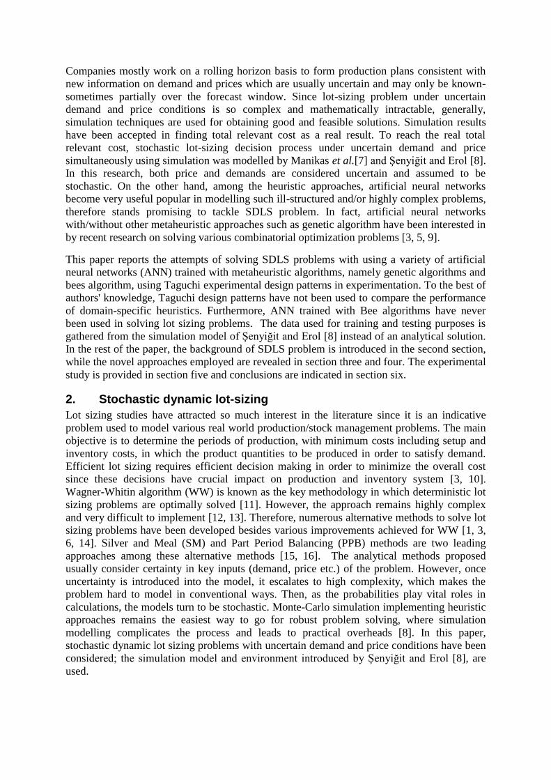
for training purposes and a simulation for data cultivation. Figure 1 depicts the system

architecture in which the FF-NN models are configured, trained and tested alongside a

simulation module. Since the probabilistic and variable properties of the system can easily be

developed and handled using simulation, the data sets for training and testing FF-NNs are

generated using simulation. The FF-NN models are configured as 3-layer feed-forward neural

networks, where a learning algorithm is selected from the Learning Algorithms Base and

applied. Here, three algorithms are included in the learning algorithms base: back propagation

(BP), genetic algorithm (GA) and bee algorithm (BA). BP is the classical gradient search-

based learning algorithm calculates the error of the system and propagates it back to the

weights of the connections of the network. On the other hand, both GA and BA are population

based heuristic search algorithms used for optimisation purposes. The aim of using them in

this study is to optimise the weights of the connections form the network so that the FF-NN

model can predict the cost of lot-sizing system with minimum error. Once a learning

algorithm is preferred, the configuration of FF-NN model is completed, then, the model is

trained using the samples included in training data-set fetched from the Data Set unit, where

the simulation results sampled in. The training phase is conducted until a certain level of

learning is achieved. After that, another data-set is retrieved to test FF-NN’s performance.

Figure 1: The complete system architecture

As declared before, the main purpose of this study is to find the optimal lot-size (amount of

order) that minimizes total relevant cost under price and demand uncertainties. The cost study

was carried out comparatively to identify which heuristic approach for costing would be most

appropriate and relevant in performance analysis. Using simulation results, costing

heuristics/techniques known as revised silver meal (RSM), revised least unit cost (RLUC),

cost benefit (CB) have been chosen [8]. Then, the following four modelling approaches,

called Taguchi Design of Experiment (TDOE), FF-NN model trained with back propagation

(BP), FF-NN model with GA and FF-NN with BA, have been implemented to solve SDLS

problems. At the first stage, CB, RLUC, RSM costing methods are compared with one

another with respect to the minimum total relevant cost based on simulation results using

TDOE approach. As a result, RLUC method is selected for evaluation since it provides the

higher correlation and lower error. Then, the problem is studied with TDOE starting with the

modelling information to be considered as the system inputs with degrees of freedom, where

each set of them reflects a unique state of the problem. Once identified, the set of inputs are

fed in to the neural network models to find out system’s response/output. Since the ultimate

objective is to predict the lot-sizes with minimum error, the problem is modelled as a

minimisation problem subsequently; the aim is set to “the smaller the difference is the better”.

Afterwards, Taguchi orthogonal arrays are considered to be used as sampling templates for

setting up experimentation needed for both training and testing sets of FF-NN models. Once

selected, then the BP, GA and BA models are trained and tested accordingly. Use of Taguchi

OA’s for sampling and collecting training sets of ANN’s has been proposed by Öztemel and

Aydin [20].

The distinctive part of this study is to use variable and stochastic price and demands. It is

assumed that the demand in each period is normally distributed, where the mean rate of

demand and price vary from period to period. The coefficient of variation is constant over

time to use cumulative distribution of demand [21]. It is a well-known and widely-used

assumption in the literature [8,21,22,23,24]. Also, price is a uniform random variable for ease

of understanding as it is assumed in Manikas et al. [7]. Unit holding cost does not depend on

purchasing price. Li et al [25] determined the quantities that have to be re-manufactured at

each period to minimise the total relevant cost. Brandimarte [26] proposed a heuristic solution

approach for dynamic lot-sizing problem production plans which were applied in a realistic

rolling horizon framework.

The assumptions in this work are analogous to Bookbinder and Tan [21] with some

differences. We assumed that purchasing price is non-stationary and stochastic as demand is.

The total relevant cost is calculated as the sum of costs consisting of purchasing cost, set-up

cost, holding cost, and lost sale cost. The following assumptions are used in modelling non-

stationary stochastic inventory system in the simulation of this study, which are apparently

more realistic.

i. The demand and price of raw material for periods are mutually independent random

variables. Demand sizes are assumed to be normal random variables, and prices are

uniform random variables.

ii. Expected value for demand size and price are required before making lot sizing

decisions.

iii. Non-stationary demand and price patterns are permitted.

iv. Lot sizing decisions are made on a rolling horizon basis.

v. Partial or complete lost sale are permitted.

vi. Order lead time is zero.

4. Learning with Genetic algorithms (GA) and Bees Algorithm (BA)

The need for an improved learning approach over the fundamental back-propagation

algorithm is due to its coarse-grained approximation to find the most appropriate weights so

as to estimate the outputs as accurate as possible. Various gradient-based approaches have

been proposed to overcome this shortcoming. Among these are the metaheuristic approaches

such as genetic algorithms [27,28,29], particle swarm optimisation and artificial bee colony

algorithms [30,31,32]. In this paper, we report the performance of two attempted approaches:

genetic algorithm, and bee algorithm.

Genetic algorithms (GA) are of very well-known metaheuristic approaches used in

optimisation, which have a strong record of success in solving difficult problems such as NP-

Hard ones. That encourages researchers to use it for solving various problems. Among these

is the training of ANN models, which appears as the problem of finding the optimum set of

weights, which makes the ANN models best-learned and interpolate/extrapolate values

expected. Chan et al [27,28] have proposed a cutting edge GA approach for training ANN

models, while an early and comprehensive review on evolutionary neural networks is

provided by Yao [29].

Artificial bee colony-based algorithms are of swarm intelligence algorithms developed

recently, which are inspired of the social behaviour of the natural bee colonies [33]. This

family of algorithms has been successfully used for various applications such as modelling on

communication networks, manufacturing cell formation, training artificial neural networks

[34,35,36]. The main idea behind a simple bee colony optimisation algorithm is to follow the

most successful member of the colony in conducting the search. The scenario followed is that

once a bee found a fruitful region, then it performs the waggle dance to communicate to the

rest of the colony so that a number of peer-bees come to that area for a better collective search

of food. Inspired of this natural process, bee algorithms are implemented for efficient search

methodologies borrowing this idea to direct the search to a more fruitful region of the search

space. That would result a quicker search for an appropriate solution to be considered as a

neat near-optimum. The detailed information on the bee algorithm (BA) attempted in this

research can be found in Düğenci [32].

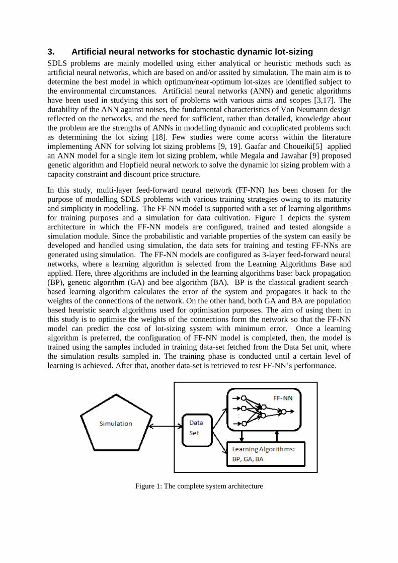
Figure 2: Learning procedures with heuristic algorithms

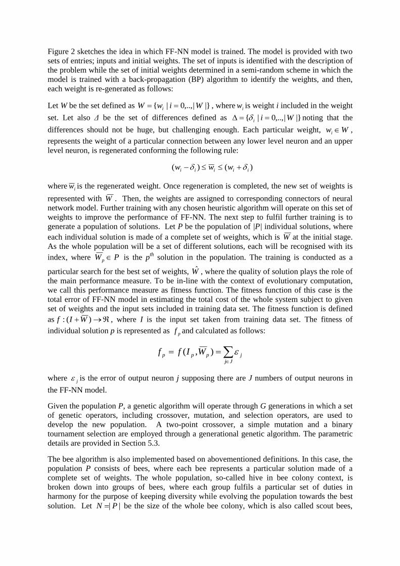
Figure 2 sketches the idea in which FF-NN model is trained. The model is provided with two

sets of entries; inputs and initial weights. The set of inputs is identified with the description of

the problem while the set of initial weights determined in a semi-random scheme in which the

model is trained with a back-propagation (BP) algorithm to identify the weights, and then,

each weight is re-generated as follows:

Let W be the set defined as ||,..,0| WiwW i , where iw is weight i included in the weight

set. Let also Δ be the set of differences defined as ||,..,0| Wii noting that the

differences should not be huge, but challenging enough. Each particular weight, Wwi ,

represents the weight of a particular connection between any lower level neuron and an upper

level neuron, is regenerated conforming the following rule:

)()( iiiii www

where iw is the regenerated weight. Once regeneration is completed, the new set of weights is

represented with W . Then, the weights are assigned to corresponding connectors of neural

network model. Further training with any chosen heuristic algorithm will operate on this set of

weights to improve the performance of FF-NN. The next step to fulfil further training is to

generate a population of solutions. Let P be the population of |P| individual solutions, where

each individual solution is made of a complete set of weights, which is W at the initial stage.

As the whole population will be a set of different solutions, each will be recognised with its

index, where PWp is the pth

solution in the population. The training is conducted as a

particular search for the best set of weights, W , where the quality of solution plays the role of

the main performance measure. To be in-line with the context of evolutionary computation,

we call this performance measure as fitness function. The fitness function of this case is the

total error of FF-NN model in estimating the total cost of the whole system subject to given

set of weights and the input sets included in training data set. The fitness function is defined

as )(: WIf , where I is the input set taken from training data set. The fitness of

individual solution p is represented as pf and calculated as follows:

Jj

jppp WIff ),(

where j is the error of output neuron j supposing there are J numbers of output neurons in

the FF-NN model.

Given the population P, a genetic algorithm will operate through G generations in which a set

of genetic operators, including crossover, mutation, and selection operators, are used to

develop the new population. A two-point crossover, a simple mutation and a binary

tournament selection are employed through a generational genetic algorithm. The parametric

details are provided in Section 5.3.

The bee algorithm is also implemented based on abovementioned definitions. In this case, the

population P consists of bees, where each bee represents a particular solution made of a

complete set of weights. The whole population, so-called hive in bee colony context, is

broken down into groups of bees, where each group fulfils a particular set of duties in

harmony for the purpose of keeping diversity while evolving the population towards the best

solution. Let || PN be the size of the whole bee colony, which is also called scout bees,

and M be the number of sites visited/searched by the scouts. There are E numbers of sites

found very valuable to search in depth, which are called elite sites and considered as a subset

of the searched sites, ME . The total number of bees recruited on elite sites is En , which

is calculated as

Ei

iE en , where ie is the number of bees recruited per elite site. The non-

elite sites, EM , are also assigned with bees from the colony, which can be represented as

EMn and calculated as

EMi

iEM en , where ie is the number of bees deployed on non-elite

site i. In addition to abovementioned sites, a number of bees are assigned to carry on random

search around the hive in order to keep diversity and keep up with aspiration. The number of

this group of bees is represented with on such that oEME nnnN . The new-born bees are

generated using a neighbourhood function, ii WWNF : , which randomly alternates a new

set of weights. In this particular case, NF is implemented to revise the weights with

ii ww , where ρ is a random number varies in the range of [-1,1] while γ is the

granularity coefficient, which normalizes the amount of change. NF is also used as the

mutation operator in GA implementation. The BA first initialises all abovementioned

parameters and determines the fitness of each bee within the colony, then sorts them in a

particular order. Afterward, it repeats (i) identifying the elite sites and sending addition teams

of bees to each one, (ii) identifying non-elite sites, and recruiting corresponding teams on

each, (iii) generates a set of new-born bees, and finally (iv) evaluating the fitness of every bee.

This set of actions is iterated up to satisfaction of a predefined criterion.

5. Experimental Results

In this paper, the multi-period single-item lot sizing problem under stochastic environment

with demand and price uncertainties is solved with FF-NN models. The uncertainties

considered with price and demand, are in terms of raw material, which makes the problem the

same as stochastic lot sizing problem. First of all, three simulation models have been

developed using ARENA simulation package implementing three problem solving heuristics;

Revised Least Unit Cost (RLUC), Revised Silver-Meal (RSM) and Cost Benefit (CB),

respectively. For the purpose of verification, the simulated models have been run with some

realistic data and cleared of verification. Both RLUC and RSM heuristics are the modified

versions of well-known heuristics called Silver-Meal and Least-Unit Cost while the Cost-

Benefit is based on a cost-benefit evaluation at decision points [8]. The simulation models

have been run and results collected for all three heuristics for comparative purpose. The

comparisons are conducted using TDOE method, which resulted in that the outperforming

heuristic is found as RLUC. Following these initial experimentations, we generated a data set

of totally 129 values (102 used for training and 27 used for testing) for configuring, training

and testing TDOE, BP, GA, and BA models. Following is the details provided.

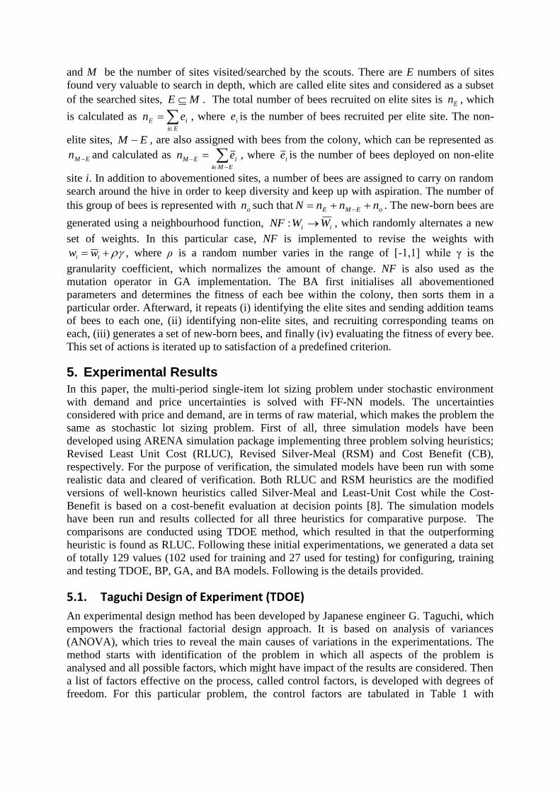
5.1. Taguchi Design of Experiment (TDOE)

An experimental design method has been developed by Japanese engineer G. Taguchi, which

empowers the fractional factorial design approach. It is based on analysis of variances

(ANOVA), which tries to reveal the main causes of variations in the experimentations. The

method starts with identification of the problem in which all aspects of the problem is

analysed and all possible factors, which might have impact of the results are considered. Then

a list of factors effective on the process, called control factors, is developed with degrees of

freedom. For this particular problem, the control factors are tabulated in Table 1 with

corresponding possible levels. The aim of SDLS problem is to minimise the total system cost

calculated with RLUC, which can be considered as the main objective of model.

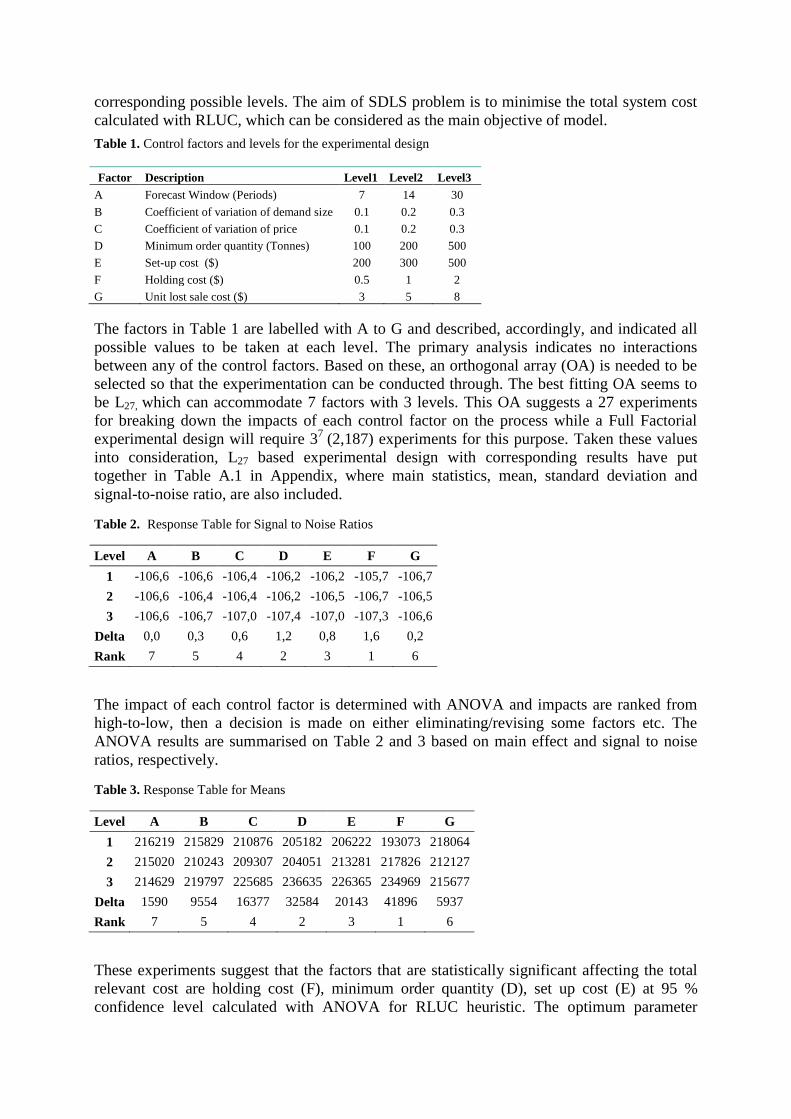
Table 1. Control factors and levels for the experimental design

Factor Description Level1 Level2 Level3

A Forecast Window (Periods) 7 14 30

B Coefficient of variation of demand size 0.1 0.2 0.3

C Coefficient of variation of price 0.1 0.2 0.3

D Minimum order quantity (Tonnes) 100 200 500

E Set-up cost ($) 200 300 500

F Holding cost ($) 0.5 1 2

G Unit lost sale cost ($) 3 5 8

The factors in Table 1 are labelled with A to G and described, accordingly, and indicated all

possible values to be taken at each level. The primary analysis indicates no interactions

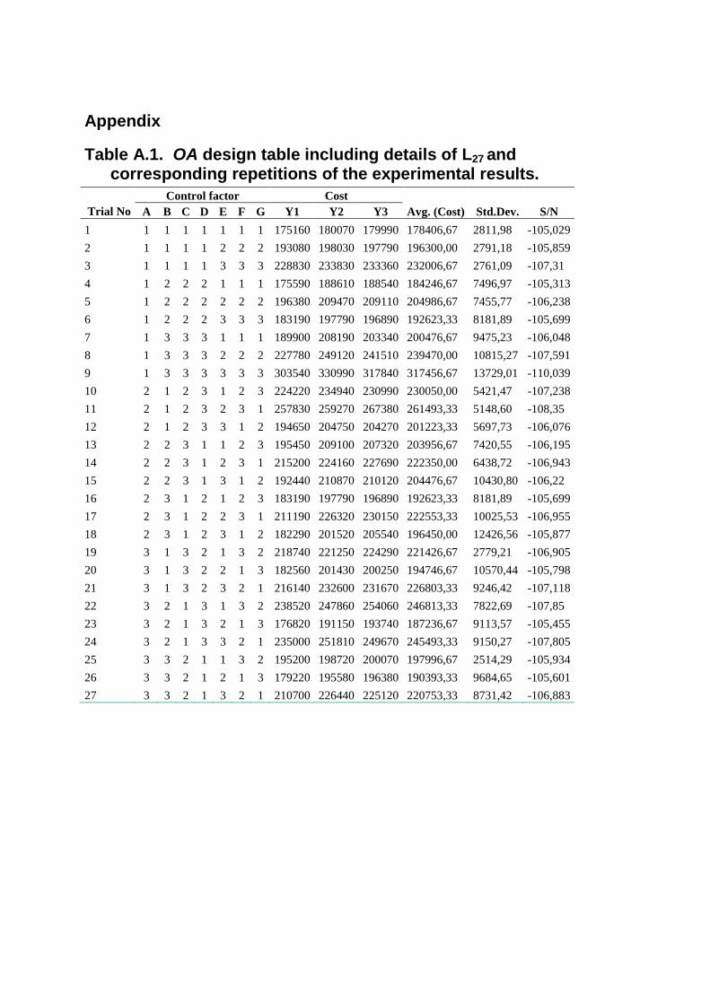
between any of the control factors. Based on these, an orthogonal array (OA) is needed to be

selected so that the experimentation can be conducted through. The best fitting OA seems to

be L27, which can accommodate 7 factors with 3 levels. This OA suggests a 27 experiments

for breaking down the impacts of each control factor on the process while a Full Factorial

experimental design will require 37

(2,187) experiments for this purpose. Taken these values

into consideration, L27 based experimental design with corresponding results have put

together in Table A.1 in Appendix, where main statistics, mean, standard deviation and

signal-to-noise ratio, are also included.

Table 2. Response Table for Signal to Noise Ratios

Level A B C D E F G

1 -106,6 -106,6 -106,4 -106,2 -106,2 -105,7 -106,7

2 -106,6 -106,4 -106,4 -106,2 -106,5 -106,7 -106,5

3 -106,6 -106,7 -107,0 -107,4 -107,0 -107,3 -106,6

Delta 0,0 0,3 0,6 1,2 0,8 1,6 0,2

Rank 7 5 4 2 3 1 6

The impact of each control factor is determined with ANOVA and impacts are ranked from

high-to-low, then a decision is made on either eliminating/revising some factors etc. The

ANOVA results are summarised on Table 2 and 3 based on main effect and signal to noise

ratios, respectively.

Table 3. Response Table for Means

Level A B C D E F G

1 216219 215829 210876 205182 206222 193073 218064

2 215020 210243 209307 204051 213281 217826 212127

3 214629 219797 225685 236635 226365 234969 215677

Delta 1590 9554 16377 32584 20143 41896 5937

Rank 7 5 4 2 3 1 6

These experiments suggest that the factors that are statistically significant affecting the total

relevant cost are holding cost (F), minimum order quantity (D), set up cost (E) at 95 %

confidence level calculated with ANOVA for RLUC heuristic. The optimum parameter

setting can be concluded as A3B2C2D2E1F1G2 based on Table 2 and 3. The optimum setting is

validated with a confirmation experiment repeated 5 times and averaged in $174678. This

clearly confirms that the configuration of control factors are the best based on provided

information.

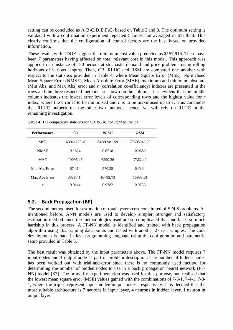
These results with TDOE suggest the minimum cost value predicted as $157,916. There have

been 7 parameters having affected on total relevant cost in this model. This approach was

applied to an instance of 150 periods at stochastic demand and price problems using rolling

horizons of various lengths. Then, CB, RLUC and RSM are compared one another with

respect to the statistics provided in Table 4, where Mean Square Error (MSE), Normalised

Mean Square Error (NMSE), Mean Absolute Error (MAE), maximum and minimum absolute

(Min Abs, and Max Abs) error and r (correlation co-efficiency) indexes are presented in the

rows and the three respected methods are shown on the columns. It is evident that the middle

column indicates the lowest error levels of corresponding rows and the highest value for r

index, where the error is to be minimised and r is to be maximised up to 1. This concludes

that RLUC outperforms the other two methods; hence, we will rely on RLUC in the

remaining investigation.

Table 4. The comparative statistics for CB, RLUC and RSM heuristics

Performance CB RLUC RSM

MSE 163911229.40 64380981.59 77503945.29

NMSE 0.1824 0.0518 0.0680

MAE 10096.46 6290.36 7362.40

Min Abs Error 674.14 570.25 645.34

Max Abs Error 33387.14 16782.73 15933.61

r 0.9144 0.9782 0.9756

5.2. Back Propagation (BP) The second method used for estimation of total system cost constituted of SDLS problems. As

mentioned before, ANN models are used to develop simpler, stronger and satisfactory

estimation method since the methodologies used are so complicated that one faces so much

hardship in this process. A FF-NN model is identified and trained with back propagation

algorithm using 102 training data points and tested with another 27 test samples. The code

development is made in Java programming language using the configuration and parametric

setup provided in Table 5.

The best result was obtained by the input parameters above. The FF-NN model requires 7

input nodes and 1 output node as part of problem description. The number of hidden nodes

has been worked out with trial-and-error since there is no commonly used method for

determining the number of hidden nodes to use in a back propagation neural network (FF-

NN) model [37]. The primarily experimentation was used for this purpose, and realised that

the lowest mean square error (MSE) values gained with the combinations of 7-3-1, 7-4-1, 7-8-

1, where the triples represent input-hidden-output nodes, respectively. It is decided that the

most suitable architecture is 7 neurons in input layer, 4 neurons in hidden layer, 1 neuron in

output layer.

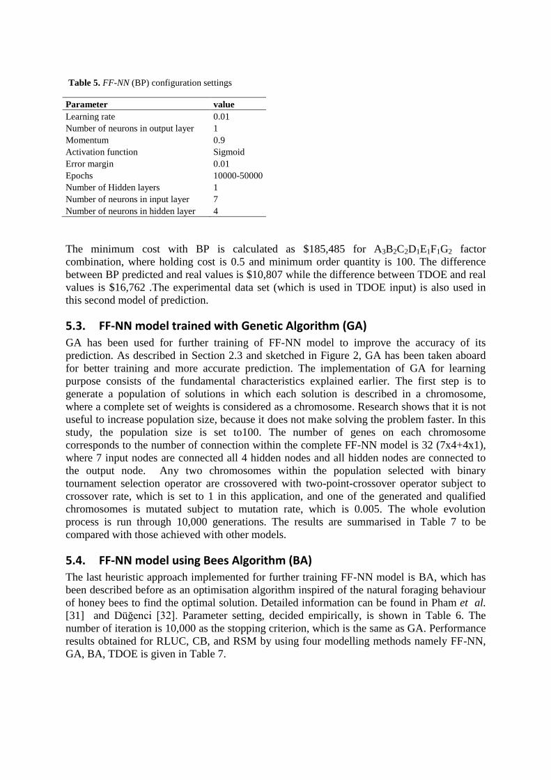
Table 5. FF-NN (BP) configuration settings

Parameter value

Learning rate 0.01

Number of neurons in output layer 1

Momentum 0.9

Activation function Sigmoid

Error margin 0.01

Epochs 10000-50000

Number of Hidden layers 1

Number of neurons in input layer 7

Number of neurons in hidden layer 4

The minimum cost with BP is calculated as $185,485 for A3B2C2D1E1F1G2 factor

combination, where holding cost is 0.5 and minimum order quantity is 100. The difference

between BP predicted and real values is $10,807 while the difference between TDOE and real

values is $16,762 .The experimental data set (which is used in TDOE input) is also used in

this second model of prediction.

5.3. FF-NN model trained with Genetic Algorithm (GA)

GA has been used for further training of FF-NN model to improve the accuracy of its

prediction. As described in Section 2.3 and sketched in Figure 2, GA has been taken aboard

for better training and more accurate prediction. The implementation of GA for learning

purpose consists of the fundamental characteristics explained earlier. The first step is to

generate a population of solutions in which each solution is described in a chromosome,

where a complete set of weights is considered as a chromosome. Research shows that it is not

useful to increase population size, because it does not make solving the problem faster. In this

study, the population size is set to100. The number of genes on each chromosome

corresponds to the number of connection within the complete FF-NN model is 32 (7x4+4x1),

where 7 input nodes are connected all 4 hidden nodes and all hidden nodes are connected to

the output node. Any two chromosomes within the population selected with binary

tournament selection operator are crossovered with two-point-crossover operator subject to

crossover rate, which is set to 1 in this application, and one of the generated and qualified

chromosomes is mutated subject to mutation rate, which is 0.005. The whole evolution

process is run through 10,000 generations. The results are summarised in Table 7 to be

compared with those achieved with other models.

5.4. FF-NN model using Bees Algorithm (BA) The last heuristic approach implemented for further training FF-NN model is BA, which has

been described before as an optimisation algorithm inspired of the natural foraging behaviour

of honey bees to find the optimal solution. Detailed information can be found in Pham et al.

[31] and Düğenci [32]. Parameter setting, decided empirically, is shown in Table 6. The

number of iteration is 10,000 as the stopping criterion, which is the same as GA. Performance

results obtained for RLUC, CB, and RSM by using four modelling methods namely FF-NN,

GA, BA, TDOE is given in Table 7.

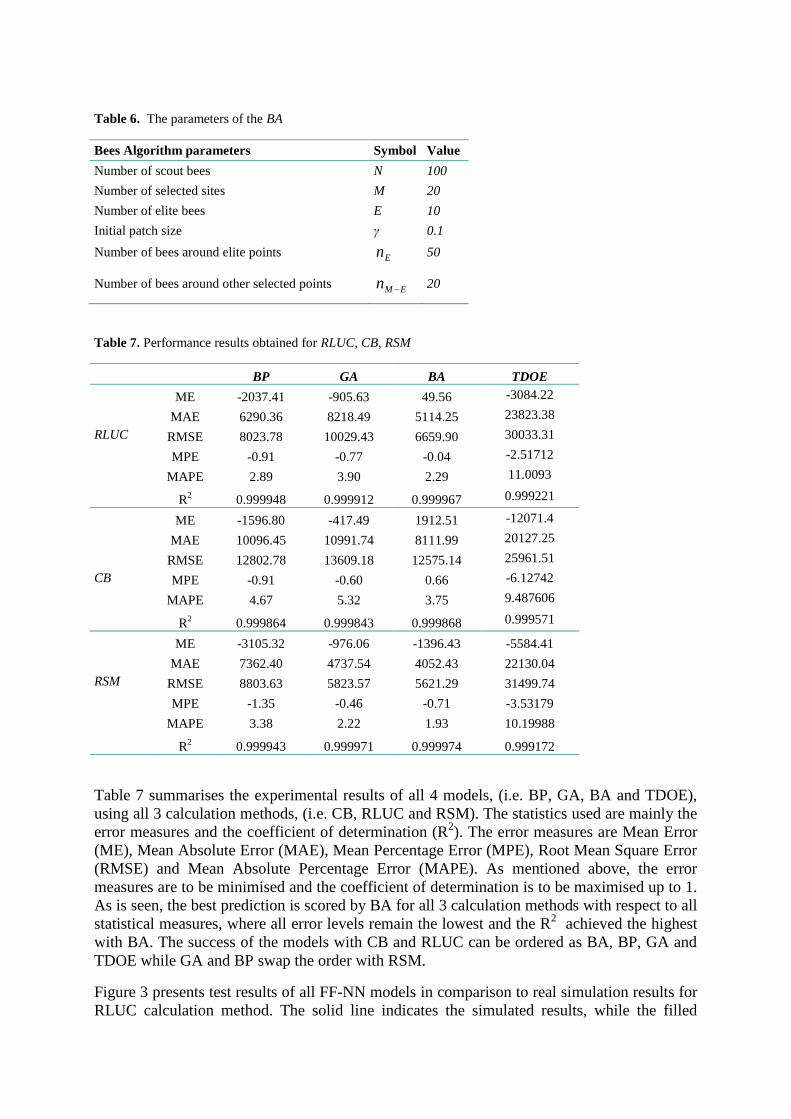
Table 6. The parameters of the BA

Bees Algorithm parameters Symbol Value

Number of scout bees N 100

Number of selected sites M 20

Number of elite bees E 10

Initial patch size γ 0.1

Number of bees around elite points En 50

Number of bees around other selected points EMn 20

Table 7. Performance results obtained for RLUC, CB, RSM

BP GA BA TDOE

ME -2037.41 -905.63 49.56 -3084.22

MAE 6290.36 8218.49 5114.25 23823.38

RLUC RMSE 8023.78 10029.43 6659.90 30033.31

MPE -0.91 -0.77 -0.04 -2.51712

MAPE 2.89 3.90 2.29 11.0093

R2

0.999948 0.999912 0.999967 0.999221

ME -1596.80 -417.49 1912.51 -12071.4

MAE 10096.45 10991.74 8111.99 20127.25

RMSE 12802.78 13609.18 12575.14 25961.51

CB MPE -0.91 -0.60 0.66 -6.12742

MAPE 4.67 5.32 3.75 9.487606

R2

0.999864 0.999843 0.999868 0.999571

ME -3105.32 -976.06 -1396.43 -5584.41

MAE 7362.40 4737.54 4052.43 22130.04

RSM RMSE 8803.63 5823.57 5621.29 31499.74

MPE -1.35 -0.46 -0.71 -3.53179

MAPE 3.38 2.22 1.93 10.19988

R2

0.999943 0.999971 0.999974 0.999172

Table 7 summarises the experimental results of all 4 models, (i.e. BP, GA, BA and TDOE),

using all 3 calculation methods, (i.e. CB, RLUC and RSM). The statistics used are mainly the

error measures and the coefficient of determination (R2). The error measures are Mean Error

(ME), Mean Absolute Error (MAE), Mean Percentage Error (MPE), Root Mean Square Error

(RMSE) and Mean Absolute Percentage Error (MAPE). As mentioned above, the error

measures are to be minimised and the coefficient of determination is to be maximised up to 1.

As is seen, the best prediction is scored by BA for all 3 calculation methods with respect to all

statistical measures, where all error levels remain the lowest and the R2 achieved the highest

with BA. The success of the models with CB and RLUC can be ordered as BA, BP, GA and

TDOE while GA and BP swap the order with RSM.

Figure 3 presents test results of all FF-NN models in comparison to real simulation results for

RLUC calculation method. The solid line indicates the simulated results, while the filled

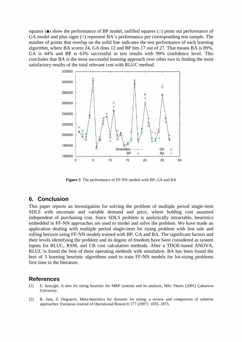
squares () show the performance of BP model, unfilled squares () point out performance of

GA model and plus signs (+) represent BA’s performance per corresponding test sample. The

number of points that overlap on the solid line indicates the test performance of each learning

algorithm, where BA scores 24, GA does 12 and BP hits 17 out of 27. That means BA is 89%,

GA is 44% and BP is 63% successful in test results with 99% confidence level. This

concludes that BA is the most successful learning approach over other two in finding the most

satisfactory results of the total relevant cost with RLUC method.

Figure 3 The performance of FF-NN models with BP, GA and BA

6. Conclusion

This paper reports an investigation for solving the problem of multiple period single-item

SDLS with uncertain and variable demand and price, where holding cost assumed

independent of purchasing cost. Since SDLS problem is analytically intractable, heuristics

embedded in FF-NN approaches are used to model and solve the problem. We have made an

application dealing with multiple period single-item lot sizing problem with lost sale and

rolling horizon using FF-NN models trained with BP, GA and BA. The significant factors and

their levels identifying the problem and its degree of freedom have been considered as system

inputs for RLUC, RSM, and CB cost calculation methods. After a TDOE-based ANOVA,

RLUC is found the best of three operating methods with simulation. BA has been found the

best of 3 learning heuristic algorithms used to train FF-NN models for lot-sizing problems

first time in the literature.

References [1] E. Şenyiğit, A new lot sizing heuristic for MRP systems and its analysis, MSc Thesis (2001) Çukurova

University.

[2] R. Jans, Z. Degraeve, Meta-heuristics for dynamic lot sizing: a review and comparison of solution

approaches. European Journal of Operational Research 177 (2007) 1855–1875.

[3] H.G. Gören, S. Tunali, R. Jans, A review of applications of genetic algorithms in lot sizing, Journal of

Intelligent Manufacturing, Vol. 21, (2010), 575-590.

[4] H.C. Bahl, L.P. Ritzman, J.N.D Gupta, Determining lot sizes and resource requirements: a review,

Operations Research 35 (1987) 329–345.

[5] L.K. Gaafar, M.H. Choueiki, A neural network model for solving the lot sizing problem, The International

Journal of Management Science, Omega Vol. 28 (2000) 175-184.

[6] U. Atici, Lot-sizing by using artificial neural network. MSc Thesis (2011) Erciyes University.

[7] A. Manikas, Y. Chang, M. Ferguson, BlueLinx can benefit from innovative inventory management

methods for commodity forward buys, Omega 37 (2009) 545–554.

[8] E. Şenyiğit, R. Erol, New lot sizing heuristics for demand and price uncertainties with service-level

constraint, International Journal of Production Research 48 (2010) 21-44.

[9] N. Megala, N. Jawahar, Genetic algorithm and Hopfield neural network for a dynamic lot sizing problem,

International Journal of Advanced Manufacturing Technology 27 (2006) 1178-1191.

[10] G. Marco, T. Marco, Neural networks in production planning and control, Production Planning &

Control 10 (4) (1999) 324 -339.

[11] H.M. Wagner, T.M. Whitin, Dynamic version of the economic lot size model, Management Science (5)

(1958) 89-96.

[12] E.A. Silver, H.C. Meal, A heuristic for selecting lot size quantities for the case of a deterministic time

varying demand rate and discrete opportunities for replenishment, Production Inventory Management 14

(2) (1973) 64-74.

[13] E.A. Silver, R. Peterson, Decision systems for inventory management and Production Planning (1985)

New York: Wiley.

[14] M. Chen, S. C. Sarin, A. Peake, Integrated lot sizing and dispatching in wafer Fabrication, Production

Planning & Control 21 ( 5), (2010) 485-495.

[15] J.J. De Matteis, A.G. Mendoza, An economic lot sizing technique, IBM systems journal 7 (1968) 30-46.

[16] J. Orlicky, Material Requirement Planning (1974) New York: McGraw Hill.

[17] N.H.M. Radzi, H. Haron, T.I.T. Jahori, Lot Sizing Using Neural Network Approach, Proceedings of the

2nd

IMT-GT Regional Conference on Mathematics, Statistic and Applications Universiti Sains Malaysia

Penang (2000) June 13-15.

[18] K.J. Anil, J. Mao, K.M. Mohiuddin, Artificial Neural Network: A Tutorial, IBM Almaden Research

Centre, Michigan, Michigan State University (1996) 1-14.

[19] E.H.L. Aarts, M.F. Reijnhoudt, H.P. Stehouwer, J. Wessels, A Novel Decomposition Approach for on-

line lot-sizing. European Journal of Operational Research 122 (2000) 339–353.

[20] E. Öztemel, M.E. Aydin, An artificial neural network-based experimental design method”, Journal of

Turkish Environment and Engineering, (1996) 20(2).

[21] J.H. Bookbinder, J.Y. Tan, Strategies for the probabilistic lot sizing problem with service level

constraints, Management Science 34 (1988) 1096–1108.

[22] S.A.Tarim, B.G. Kingsman, The stochastic dynamic production/inventory lot sizing problem with

service-level constraints, International Journal of Production Economics 88 (2004) 105–119.

[23] S.A. Tarim, B.G. Kingsman, Modelling and computing (Rn,Sn) policies for inventory systems with non-

stationary stochastic demand, European Journal of Operational Research 174 (2006) 581–599.

[24] S.A. Tarim, B.M. Smith, Constraint programming for computing non-stationary (R, S) inventory

systems, European Journal of Operational Research 189 (2008) 1004–1021.

[25] C. Li, F. Liu, H. Cao, Q. Wang, A stochastic dynamic programming based model for uncertain production

planning of re-manufacturing system, International Journal of Production Research 47 (13) (2009) 3657 -

3668.

[26] P. Brandimarte, Multi-item capacitated lot-sizing with demand uncertainty, International Journal of

Production Research 44 (15) (2006) 2997 – 3022.

[27] K.Y. Chan, C.K. Kwong, X.G. Luo, Improved orthogonal array based simulated annealing with

interaction analysis between variables for design optimization, Expert Systems with Applications 36(4)

(2009) 7379-7389.

[28] K.Y. Chan, C.K. Kwong, H. Jiang, M.E. Aydin, T.C. Fogarty, A new orthogonal array based crossover,

with analysis of gene interactions, for evolutionary algorithms and its application to car door design,

Expert Systems with Applications 37(5) (2010) 3853-3862.

[29] X. Yao, A review of evolutionary artificial neural networks, International Journal of Intelligent Systems,

8 (1993) 539–567.

[30] Y. Da, G. Xiurun, An improved PSO-based ANN with simulated annealing technique, Neurocomputing,

63 (2005) 527-533.

[31] D. T. Pham, S. Otri, A. Ghanbarzadeh, E. Koc, Application of the bees algorithm to the training of

learning vector quantisation networks for control chart pattern recognition. Proceedings of the

Information and Communication Technologies (ICTTA’06) 1624–1629 (2006). Syria.

[32] M. Düğenci, Using the bee’s algorithm for artificial neural Networks training and the control application

of wastewater treatment plant (2007) Thesis (PhD). Sakarya University.

[33] D.Karaboga, B. Akay, A Survey: Algorithms Simulating Bee Swarm Intelligence, Artificial Intelligence

Review 31 (1) (2009) 68-85.

[34] M. Farooq, Bee-inspired protocol engineering: From nature to networks. Berlin, Heidelberg, (2008)

Germany: Springer.

[35] D. T. Pham, A. Afify, E.Koc, Manufacturing cell formation using the Bees Algorithm. IPROMS’2007

Innovative Production Machines and Systems Virtual Conference Cardiff (2007) UK.

[36] D.T. Pham, A. Ghanbarzadeh, E. Koç, S. Otri, S. Rahim, M. Zaid, The Bees algorithm-A Novel Tool for

Complex Optimisation Problems, IPROMS’2006 Intelligent Production Machines and Systems, (2006)

454-459.

[37] C.C. Chiu, C.T. Su, G.S. Yang, J-S. Huang, S-C. Chen, N-T. Cheng, Selection of optimal parameters in

gas-assisted injection moulding using a neural network model and the Taguchi method, International

Journal of Quality Science 2 (2) (1997) 106-120.

Appendix

Table A.1. OA design table including details of L27 and corresponding repetitions of the experimental results.

Control factor Cost

Trial No A B C D E F G Y1 Y2 Y3 Avg. (Cost) Std.Dev. S/N

1 1 1 1 1 1 1 1 175160 180070 179990 178406,67 2811,98 -105,029

2 1 1 1 1 2 2 2 193080 198030 197790 196300,00 2791,18 -105,859

3 1 1 1 1 3 3 3 228830 233830 233360 232006,67 2761,09 -107,31

4 1 2 2 2 1 1 1 175590 188610 188540 184246,67 7496,97 -105,313

5 1 2 2 2 2 2 2 196380 209470 209110 204986,67 7455,77 -106,238

6 1 2 2 2 3 3 3 183190 197790 196890 192623,33 8181,89 -105,699

7 1 3 3 3 1 1 1 189900 208190 203340 200476,67 9475,23 -106,048

8 1 3 3 3 2 2 2 227780 249120 241510 239470,00 10815,27 -107,591

9 1 3 3 3 3 3 3 303540 330990 317840 317456,67 13729,01 -110,039

10 2 1 2 3 1 2 3 224220 234940 230990 230050,00 5421,47 -107,238

11 2 1 2 3 2 3 1 257830 259270 267380 261493,33 5148,60 -108,35

12 2 1 2 3 3 1 2 194650 204750 204270 201223,33 5697,73 -106,076

13 2 2 3 1 1 2 3 195450 209100 207320 203956,67 7420,55 -106,195

14 2 2 3 1 2 3 1 215200 224160 227690 222350,00 6438,72 -106,943

15 2 2 3 1 3 1 2 192440 210870 210120 204476,67 10430,80 -106,22

16 2 3 1 2 1 2 3 183190 197790 196890 192623,33 8181,89 -105,699

17 2 3 1 2 2 3 1 211190 226320 230150 222553,33 10025,53 -106,955

18 2 3 1 2 3 1 2 182290 201520 205540 196450,00 12426,56 -105,877

19 3 1 3 2 1 3 2 218740 221250 224290 221426,67 2779,21 -106,905

20 3 1 3 2 2 1 3 182560 201430 200250 194746,67 10570,44 -105,798

21 3 1 3 2 3 2 1 216140 232600 231670 226803,33 9246,42 -107,118

22 3 2 1 3 1 3 2 238520 247860 254060 246813,33 7822,69 -107,85

23 3 2 1 3 2 1 3 176820 191150 193740 187236,67 9113,57 -105,455

24 3 2 1 3 3 2 1 235000 251810 249670 245493,33 9150,27 -107,805

25 3 3 2 1 1 3 2 195200 198720 200070 197996,67 2514,29 -105,934

26 3 3 2 1 2 1 3 179220 195580 196380 190393,33 9684,65 -105,601

27 3 3 2 1 3 2 1 210700 226440 225120 220753,33 8731,42 -106,883