Heuristic Search and Information Visualization Methods for School Redistricting

Marie desJardins, Blazej Bulka, Ryan Carr, Eric Jordan, and Penny RheingansDepartment of Computer Science and Electrical Engineering

University of Maryland Baltimore County1000 Hilltop Circle, Baltimore MD 21250

{mariedj,bulka1,carr2,ejordan1,rheingan}@umbc.edu

Abstract

We describe an application of AI search and information visu-alization techniques to the problem of school redistricting, inwhich students are assigned to home schools within a countyor school district. This is a multicriteria optimization prob-lem in which competing objectives must be considered, suchas school capacity, busing costs, and socioeconomic distri-bution. Because of the complexity of the decision-makingproblem, tools are needed to help end users generate, evalu-ate, and compare alternative school assignment plans. A keygoal of our research is to aid users in finding multiple qual-itatively different redistricting plans that represent differenttradeoffs in the decision space.We present heuristic search methods that can be used to find aset of qualitatively different plans, and give empirical resultsof these search methods on population data from the schooldistrict of Howard County, Maryland. We show the resultingplans using novel visualization methods that we have devel-oped for summarizing and comparing alternative plans.

Motivation and OverviewThis research focuses on developing decision support toolsfor the problem of school redistricting. In this domain, thegoal is to assign the students from each geographic region(neighborhood or planning polygon) in a county or schooldistrict to a home school at each level (elementary, middle,and high school). We are working with the Howard County,Maryland, school system to develop tools that will aid ingenerating, evaluating, and comparing alternative school as-signment plans. Related applications include emergency re-sponse planning, urban planning and zoning, robot explo-ration planning, and political redistricting.

The school assignment plan should ideally satisfy a num-ber of different goals, such as meeting school capacities,balancing socioeconomic and test score distributions at theschools, minimizing busing costs, and allowing students inthe “walk area” of a school to attend that home school. Sincethese objectives are often at odds with each other, finding thebest plan is a complex multicriteria optimization problem. Itis also often desirable to create several alternative plans forconsideration; these plans should be qualitatively different—that is, they should represent different tradeoffs among the

Copyright c© 2007, American Association for Artificial Intelli-gence (www.aaai.org). All rights reserved.

evaluation criteria. Finally, because of the complexity ofthe problem, it is difficult for users to fully understand thesetradeoffs. Therefore, developing effective visualizations isan important challenge.

The contributions of our work are (1) a computational for-mulation of the school redistricting problem as a multicri-teria optimization problem; (2) novel heuristic local searchtechniques for generating high-quality, diverse (i.e., qualita-tively different) plans; (3) visualization methods1 for com-paring alternative plans; and (4) empirical results demon-strating the effectiveness of our search methods on actualHoward County school data.

The rest of this paper is organized as follows. We firstdescribe the current redistricting process in Howard County,and present some example plan visualizations that we havedeveloped. Next, we describe the search methods andpresent empirical results comparing manually and automat-ically generated plans in terms of plan quality and diversity.Finally, we summarize related work, then present our futurework and conclusions.

Redistricting ProcessThe Howard County Public School System (HCPSS) servesa rapidly growing county in suburban Maryland. The paceof development and population growth has necessitated theopening of 25 new schools in the last 14 years, turning theadjustment of school attendance areas into an almost annualevent. Under the current process, candidate plans and fea-sibility studies are generated manually2 by school systemstaff. These plans are evaluated and refined by a committeeof citizens, then presented at regional meetings for publiccomment. A small set of candidate plans is forwarded to theSuperintendent, who presents two or three recommended al-ternatives to the Board of Education. The Board has finaldecision-making authority, and will typically select one ofthe recommended plans, sometimes making minor modifi-cations in response to concerns raised by parent groups or

1These visualization methods are summarized here; they aredescribed in detail in an earlier publication (Shanbhag, Rheingans,& desJardins 2005).

2Map-based tools are used to show the proposed school dis-tricts, and a set of spreadsheets is used to generate evaluation data.No other decision support tools are used in the current process.

staff. Note that this process is specific to Howard County;other school districts may have different processes and mod-els.

Candidate plans are evaluated according to eleven mea-sured criteria: (1) the educational benefits for students, (2)the frequency with which students are redistricted, (3) thenumber and distance of students bused, (4) the total bus-ing cost, (5) the demographic makeup and academic perfor-mance of schools, (6) the number of students redistricted,(7) the maintenance of feeder patterns (i.e., the flow of stu-dents from elementary to middle to high school), (8) changesin school capacity, (9) the impact on specialized programs,(10) the functional and operational capacity of school infras-tructure, and (11) building utilization. Some of these criteriacan be clearly quantified (e.g., building utilization and bus-ing costs), while others are harder to quantify (e.g., educa-tional benefits and impact on specialized programs).

In practice, the process is primarily driven by building uti-lization, but serious consideration is given to feeder patterns,the number of students redistricted, demographic makeup,busing costs, and the frequency with which students are re-districted. Ideally, building utilization should be between90% and 110% of program capacity and should stay in thatrange as projected population and capacity changes occur.Desired feeder patterns ensure that there is a critical massof students who move together from one school level (ele-mentary, middle, and high school) to the next. For instance,the students from a particular middle school should consti-tute at least 15% of the population of any high school thatthey feed into. Consideration of the demographic makeup ofschools helps to ensure that economically and academicallydisadvantaged children are not unnecessarily segregated intoa few schools.

The specific redistricting problem that we focus on in thispaper is one that the county faced during the 2004-2005school year, that of developing a school assignment planfor a twelfth high school (Marriotts Ridge) that opened inFall 2005. Figure 1 shows the partitioning of planning re-gions into school attendance areas before the new schoolwas opened. A colored circle shows the location of eachschool, and each planning polygon is colored according tothe high school attended. For instance, all students in thenorthwest region of the county are assigned to Glenelg HighSchool (labeled G; bright green region) in the original plan.The unused capacity at a school is shown by a black area(wedge) inside the school circle. Schools that are over ca-pacity are outlined with a ring. Glenelg is slightly undercapacity; Marriotts Ridge (labeled MR) has zero utilization(i.e., is completely black), since no students have yet beenassigned to this school in this plan; and Mt. Hebron (labeledMH; bright pink region) is significantly over capacity.

Figure 2 shows a comparison picture of two alternativeplans that include Marriotts Ridge. The school assignmentsfor the closest-school plan—generated by assigning everypolygon to the school closest to its geographic center—areindicated by the outer colored rings in each planning poly-gon. This plan provides a useful baseline, because it op-timizes both walk usage and busing costs, but may be un-desirable in terms of capacity and demographics. The in-

ner ring shows the school assignments for the recommended(“green”) plan that was recommended by the superinten-dent’s office. The “tree ring” effect allows the user to easilysee the planning polygons where the two plans make dif-ferent recommendations. Polygons with a single color areassigned to the same school in both plans.

For example, in the center of the county, several polygonsare assigned to Marriotts Ridge by the recommended plan,but to the nearby Mount Hebron (labeled MH in Figure 1),River Hill (RH), and Centennial (C) High Schools by theclosest-school plan. The inner ring (center) of these poly-gons is displayed as sky blue (Marriots Ridge); the outerring is either bright pink (Mount Hebron), dark blue (RiverHill), or orange (Centennial). Along the southeast border ofthe county, the closest-school plan assigns a number of poly-gons to Hammond High School (H: medium blue outer ring)that are assigned to Reservoir (R: green inner ring) by therecommended plan. This difference occurs because assign-ing them to Hammond would cause that school to be overcapacity; also, in this case, those polygons help to balancethe socioeconomic distribution at Reservoir.

Search MethodsThe search space for the redistricting problem is very large.For p polygons and s schools, there are

s(p−s)

possible assignments of schools to polygons (since poly-gons containing a school are constrained to be assignedto that school). Requiring that school attendance areas begeographically contiguous reduces the number of possibleplans, but the number of plans still grows exponentially withthe number of schools and polygons. Because of this com-plexity, we have chosen to use heuristic local search meth-ods, which do not guarantee optimality, but which can beused to find good solutions reasonably quickly.

Our basic approach is a two-stage process: first, we gen-erate an initial “seed” plan using one of several methods de-scribed below; second, we use local search to “hill-climb”to a local optimum. Because of the multicriteria nature ofthe redistricting problem, we have designed several differ-ent variations of hill-climbing search that can be used to findqualitatively different alternative plans in the solution space,as discussed later.

Before describing the methods for finding seed plans andfor performing local search, we first introduce the evalua-tion criteria that we use to measure the quality of a schoolassignment plan.

Evaluation CriteriaA school plan assignment can be evaluated along multi-ple dimensions. The measured criteria used by the HowardCounty schools were summarized earlier. We have definedfive quantitative criteria, f1, . . . , f5, based on these mea-sured criteria. Each of these criteria is scaled and normal-ized so that the value for a given plan will always fall in therange [0, 1], with a lower value being preferred.

Figure 1: Original 2004-2005 school assignment plan. Each planning polygon is colored according to the school to which it isassigned. School glyphs show underutilization as a “pie wedge” (percentage of black fill). Overutilization is shown by a ringoutlining the glyph; the diameter of the ring is proportional to the degree of overutilization.

Using concepts from the multiattribute decision theory lit-erature (Keeney & Raiffa 1993), a plan P1 is said to domi-nate a second plan P2 if P1 is better along some dimension,and no worse along any dimension, than P2:Dom(P1, P2) ⇔ ∃i fi(P1) < fi(P2) ∧ ∀i fi(P1) ≤ fi(P2).

Two plans are incomparable if neither plan dominates theother.

It is often desirable to define a combined score that incor-porates all of the evaluation criteria. For this purpose, weuse a simple linear combination, F :

F (P ) =∑

i

wifi(P ),

where the weights wi ∈ [0, 1] represent the relative impor-tance of each of the criteria. Since each fi ranges from 0 to1, F will range from 0 to 5.

We introduce the following notation:• Pop(p) is the number of students in planning polygon p.• Pop(s, P ) is the number of students assigned to school s

by plan P .

• Cap(s) is the capacity of school s.

• Nschools is the number of schools in the county (12 in thisparticular planning problem).

• Nstudents =∑

p Pop(p) is the number of students in thecounty.

• s(p, P ) is the school to which polygon p is assigned byplan P .

• p ∈ s refers to the set of polygons assigned to school sby a given plan. This notation is shorthand for the morespace-consuming set notation, {p : s(p, P ) = s}.

The five evaluation criteria, which are defined in the fol-lowing paragraphs, are: school capacity (f1), socioeconomicdistribution (f2), test score distribution (f3), busing costs(f4), and walk area usage (f5).

School Capacity (f1). A plan that utilizes any school atless than 90% or greater than 110% of its capacity is con-sidered to be highly undesirable. Therefore, we compute the

Figure 2: A comparison of the recommended (“green”) plan to the closest-school plan. The color of the inner and outer ringsin each planning polygon indicate the school assignments for the recommended and closest-school plan, respectively.

0

0.1

0.2

0.3

0.4

0.5

0.6

0.7

0.8

0.9

1

0 0.5 1 1.5 2

f1

Students / Capacity

Figure 3: Penalty function for school utilization.

school utilization (i.e., the ratio of proposed school enroll-ment to school capacity), and map it to a penalty functionwith its minimum at 100%. For this purpose, we used ascaled arctan function (Figure 3):

f1(P ) =

∑

s

∣

∣

∣arctan

(

σ(

1 − Pop(s,P )Cap(s)

))∣

∣

∣

π2 Nschools

0

0.1

0.2

0.3

0.4

0.5

0.6

0.7

0.8

0.9

1

0 0.2 0.4 0.6 0.8 1

f2

FARM rate for a school

Figure 4: Penalty function for socioeconomic distribution,for a county FARM rate of 0.15.

where σ is a scaling factor that causes the scaled arctan tobe equal to 0.5 when the school utilization is either 0.9 or1.1 (σ = 10.0). As seen in Figure 3, the penalty functionincreases rapidly away from the ideal capacity of 100%, andassigns high values for values that are significantly outsidethe target range, [0.9, 1.1].

Socioeconomic Distribution (f2). The school systemuses the percentage of students that qualify for free and re-duced meals (FARM) as a measure of socioeconomic dis-tribution. The goal in creating a school assignment plan isto equalize this distribution across the county: ideally, eachschool will have the same FARM rate as the county as awhole. FARM rates are given in the data on a per-polygonbasis, denoted as FARM(p). We compute FARMC , the av-erage FARM rate for the county as a whole:

FARMC =

∑

p Pop(p) FARM(p)

Nstudents

(1)

and the FARM rate for each school:

FARM(s, P ) =

∑

p∈s Pop(p) FARM(p)

Pop(s, P ). (2)

In order to penalize greater deviations from the averageFARM rate more heavily, we take the square root of the dif-ference between the school and county FARM rates (whichboth range from 0 to 1), and then average this over theschools in the county to compute the overall socioeconomicdistribution criterion:

f2(P ) =

∑

s

√

|FARM(s, P ) − FARMC |Nschools

Figure 4 shows what one school’s contribution to the f2

penalty function would look like for a county rate ofFARMC = 0.15, as a function of the school’s FARM rate,FARM(s, P ).

Test Score Distribution (f3). The test score rate is mea-sured by the percentage of students in a given polygon orschool who achieve a score at the Proficient or Advancedlevel on the Maryland State Assessment (MSA) standard-ized test. As with the FARM data, these rates are given on aper-polygon basis in the input data. This criterion is definedanalogously to f2:

f3(P ) =

∑

s

√

|MSA(s, P ) − MSAC |Nschools

,

where MSAC and MSA(s, P ) are computed as in Equa-tions 1 and 2, respectively.

Busing Costs (f4). Busing costs would be minimized bysending all students to the geographically closest school.Our evaluation criterion for busing costs is based on the“average excess busing distance”—that is, the average dis-tance traveled beyond the minimum required. To simplifythe computation, we treat each polygon as a group of stu-dents all traveling from the geometric centroid of the poly-gon. The distance from this point to the assigned schoolis calculated; we then subtract the distance to the closestschool (denoted by CS(p)) to determine the excess busingdistance. This distance is normalized by the excess busingdistance that would be needed to bus those students to the

fourth closest school (denoted by 4CS(p)).3 These compu-tations are weighted by the population of each polygon:

f4(P ) =

∑

s

∑

p∈s Pop(p) Dist(p,s)−Dist(p,CS(p))Dist(p,4CS(p))−Dist(p,CS(p))

Nstudents

Walk Area Usage (f5). It is preferable to send childrenwho are within walking distance of some school to theirneighborhood (“walk”) school. This criterion is based onthe percentage of such students who are in fact assigned to aschool within walking distance.4

f5(P ) = 1 − w′(P )

w

where w is the number of students who are within walkingdistance of the closest school:

w =∑

p: Dist(p,CS(p))≤kw

Pop(p)

and w′ is the number of students who are within walkingdistance of their assigned school:

w′(P ) =∑

p: Dist(p,s(p,P ))≤kw

Pop(p).

Generating Seed PlansIn this paper, we use two seed plans: the closest-school planand the current (“original”) redistricting plan.

The closest-school plan simply assigns each polygon tothe school that is geographically closest to the centroid ofthe polygon. This plan minimizes busing costs and allowsall students in the walk area of a school to attend that school.However, as seen in Table 1, it results in poor school uti-lization, since some schools are overcrowded and others areunderutilized. The closest-school plan also performs some-what poorly on test-score and socioeconomic distribution,since it reinforces geographic “clustering” of income levels.

The original plan, for this data set, is the high school as-signment plan before the new Marriotts Ridge High Schoolwas built. It assigns no polygons to the new high school, soits utilization is not particularly good (Table 1). However, interms of the other criteria, it is approximately as good as thefinal accepted plans.

We have also experimented with several other seed meth-ods, including random seeds, “breadth-first” assignment ofpolygons to schools, and a minimum-spanning-tree assign-ment based on distance. The latter two are similar to the

3The reasoning behind this normalization is that it there is veryrarely a need to send students further than the third closest school.As a result, normalizing by the most distant school in the countywould result in extremely small values for any “reasonable” schoolassignment, making it difficult to differentiate among alternatives.

4The walking distance, kw , depends on the age of the children;for high schools, we use 1.5 miles. Note that this computation is anapproximation, since the actual assignment of walk areas is morecomplicated, using actual distance traveled, and taking into account“walkability” (e.g., sidewalks are required, and busy streets mustbe avoided).

closest-school assignment, but make less sense to an enduser. Random seeds are useful for a baseline, but are actu-ally nonsensical from an application perspective, since thereis no geographic contiguity at all. In our preliminary ex-periments, we also found that these seeds do not yield goodsearch performance; in particular, the random seeds causethe local search to take a very long time to converge (sincethey are so far from a reasonable plan), and the resultingplans are not particularly good. Therefore, we omit thesealternatives from the results that we present here.

Local Search MethodsWe have developed and applied three basic search methods:basic hill climbing, biased hill climbing with blind bias, andbiased hill climbing with diversity bias.

Basic hill climbing. This method simply performs a vari-ation of hill climbing on the combined score, F (P ) =∑

i wifi(P ). At each step, the search algorithm considersmoving a single polygon to a different school. The branch-ing factor for this search is high (there are (s− 1)(p−s) pos-sible actions), so rather than evaluating every possible move,we consider each of these moves in a random order, and takethe first one (if any) that improves the combined score. Inother words, at each step, a random polygon is selected andassigned to a randomly selected neighboring school. If thisimproves (reduces) the combined score, then the change ismade to the plan. This process continues until a local mini-mum is reached; that is, until there is no individual polygonthat can be moved in order to improve the score.

Biased hill climbing with blind bias. Biased hill climb-ing is a novel technique that we introduce here. It usesthe notions of dominated and incomparable solutions in themulticriteria optimization space to find multiple alternativeplans. As with basic hill climbing, this search method triesto move a random polygon to a randomly selected neigh-boring school. The difference is that this move will only beaccepted if it results in a dominating plan – that is, if somefi is improved by the change, and no fi is made worse. Ifthe change is strictly worse, it is ignored. However, if thechange results in an incomparable solution (that is, one thatis better with respect to some fi, but worse with respect tosome other fj), then the resulting plan is placed on a list of“incomparable” solutions, which we refer to as I.

When a local optimum is reached in “dominated planspace,” under the blind bias option, this plan is added to thesolution list, S, then a plan is selected randomly from theincomparable solution list I and used as the seed for a newsearch. This process is repeated until a prespecified number,k, of alternative plans is found. The set of k plans, S, isreturned.

Biased hill climbing with diversity bias. This methoduses the same basic “dominated hill climbing” approach asthe previous method to find the initial solution. However, tofind subsequent solutions, a diversity bias is applied. Specif-ically, after a local optimum is found, the new seed will be

Plan f1 f2 f3 f4 f5 F

Cap. FARM MSA Bus Walk∑

fi

Closest 0.64 0.26 0.24 0.0 0.0 1.15Original 0.47 0.25 0.22 0.13 0.17 1.24Green 0.40 0.24 0.21 0.16 0.16 1.17Red 0.40 0.24 0.21 0.15 0.17 1.19Closest/Basic 0.44 0.26 0.24 0.04 0.04 1.02Closest/Blind 0.64 0.26 0.24 0.00 0.00 1.15Closest/Div 0.64 0.26 0.24 0.00 0.00 1.15Original/Basic 0.26 0.24 0.21 0.14 0.17 1.02Original/Blind 0.37 0.22 0.20 0.13 0.17 1.09Original/Div 0.44 0.23 0.20 0.11 0.12 1.10

Table 1: Average evaluation criteria values (fi and combinedscore F (with all weights wi set to 1) for seed plans andsearch results. Search results represent the average of 10runs.

the plan from the incomparable list I whose average Eu-clidean distance (in the evaluation space) from S, the localoptima found so far, is greatest. That is,

seedi+1 = argmaxP ′∈I

∑

P∈S EvalDist(P ′, P )

|S| ,

where

EvalDist(P ′, P ) =

√

∑

i

(fi(P ′) − fi(P ))2. (3)

Since each of the fi ranges from 0 to 1, the maximum pos-sible pairwise distance between any two solutions for thefive-dimensional evaluation space is

√5 = 2.24. Of course,

it is unlikely that we would find locally optimal plans withsuch extreme values, so typically the pairwise distance willbe much smaller.

Empirical ResultsIn this section, we present results using the Howard Countyschool data for the 2004–2005 redistricting process. Thefirst experiment was designed to compare the quality of theplans that are produced by different heuristic search meth-ods, using different seed plans, to those produced by the re-districting committee. The second experiment was designedto assess the diversity (with respect to the evaluation criteria)of the sets of plans produced by different search methods.

Plan Quality. In Table 1, we compare the average fi andcombined F values for the original, closest-school, recom-mended (green), and alternate (red) plans to the plan gener-ated by each search method. (The alternate plan was pro-posed by the Superintendent’s office as an alternative tothe green plan.) To generate this data, we ran each searchmethod ten times, since some of the search steps are stochas-tic. In general, the search process is heavily influenced bythe choice of seed. The results of basic hill climbing searchwhen starting from the closest-school plan does better thanthe closest-school plan with respect to capacity (f1), butstill worse on this measure than the other manually gener-ated plans (original, recommended, and alternate). Simi-larly, the search results for basic hill climbing starting with

Method Diversity f1 f2 f3 f4 f5 FBasic 0.044 0.22 0.24 0.21 0.14 0.15 0.96Weighted 0.048 0.23 0.24 0.21 0.14 0.14 0.96Blind 0.032 0.44 0.20 0.18 0.11 0.11 1.04Diversity 0.389 0.61 0.19 0.15 0.18 0.23 1.36

Table 2: Average diversity (average pairwise distance inevaluation space) and evaluation measures for differentmethods.

the closest-school plan perform much better with respect tobusing (f4) and walk usage (f5) than the other plans.

The biased hill climbing methods show a pathological be-havior when starting from the closest-school seed. Becausethe closest-school plan is already optimal with respect tobusing costs and walk area usage, the local area containsmany incomparable plans, so the search is unable to makeany progress.

The overall combined plan quality (F ) is better for all ofthe search methods than for any of the manually constructedplans. This is a good sign, since it means that we are able tofind high-quality plans using our search methods. However,we have not yet performed a user study to determine whetherplans that appear better with respect to these criteria are, infact, seen to be better by end users. The result is certainlypromising, though, since the general framework can easilybe used with different evaluation criteria that are “tuned” tothe end users’ actual preferences.

Plan Diversity. In Table 2, we compare sets of three plansgenerated by each of our search methods to a group ofhand-generated plans (recommended, alternate, and closest-school). We give the diversity (average pairwise distance inevaluation space) and the average fi and F scores for eachof the sets. All numbers are the average of 10 runs of thespecified search method, using the original plan as the seed.

Examining three manually generated plans (closest, green(recommended), and red (alternate)) gives us a baseline forthe diversity measure. The pairwise evaluation distances ofthe manually generated plans are 0.337 (closest vs. green),0.333 (closest vs. red), and 0.019 (red vs. green), for an av-erage pairwise distance of 0.223.

Not surprisingly, basic hill climbing with all weights setto 1.0 produces sets of very similar plans, with almost nodiversity (0.044 on average—”Basic” in Table 2). There-fore, we experimented with performing hill climbing threetimes, each time with different weights. (The three runs as-sign weight 1.0 to f1 (capacity), f2 (socioeconomic distri-bution), and f4 (busing costs), respectively, and weight 0.5to all of the other evaluation criteria.) This process (referredto as “weighted” in Table 2) yields only slightly higher di-versity (0.048 on average, still below the baseline).

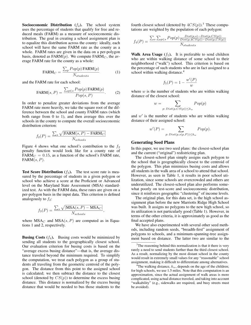
The plans using both hill climbing methods have verylow combined F values. A typical plan (with w1 = 1.0(capacity) and the other wi = 0.5) is compared to therecommended plan in Figure 5. The outer color in eachplanning polygon shows the school assigned by the recom-mended plan; the inner color shows the school assigned by

the weighted hill climbing plan. The overall F measure forthis plan is 0.91, lower than any of the manually generatedplans or any of the average search results in Table 1. Notsurprisingly, this plan performs extremely well on the ca-pacity measure (f1 = 0.20), while maintaining fairly goodperformance along the other dimensions (f2 = 0.21, f3 =0.20, f4 = 0.16, f5 = 0.15). Comparing these measuresto those given in Table 1, it is clear that this plan is bet-ter than the manually generated plans with respect to all ofthe evaluation criteria. The figure shows that the weightedhill climbing plan assigns a number of polygons to a moredistant (but still nearby) school than the recommended plan.However, although it is not stated explicitly in the evaluationcriteria, the geographic “pocketing” that this plan displays islikely to be undesirable.

Figure 6 compares three plans produced by a single rep-resentative run of weighted hill climbing. The variation inthe plans produced by the weighted hill climbing method isprimarily in the capacity, busing, and walk usage measures.Although one of the weight assignments emphasizes socioe-conomic distribution, there is not much difference in the f2

values for these plans. This may be because significantlydecreasing socioeconomic distribution would require busingstudents a very long distance, entailing a severe penalty inbusing costs and walk usage. Interestingly, two of the plansare quite similar, so only one planning polygon shows threedifferent school assignments for the three plans. (This poly-gon is in the southern part of the county, and is assigned toReservoir (green) by the first plan (outer ring), River Hill(dark blue) by the second, and Atholton (pink) by the third.)

Biased hill climbing with a blind (random) bias also givesvery little diversity (0.032 on average). However, biased hillclimbing with diversity bias gives the highest diversity ofany method, and much higher diversity than the baselineset of plans (0.389 on average). Note that this is accom-plished at some loss of quality: the average combined mea-sure (F ) for diversity-biased search is 1.36, compared to av-erages ranging from 0.96–1.04 for the other search methods.Three plans produced by a typical run of diversity-biased hillclimbing are shown in Figure 7. Although the average diver-sity is high, the three plans are not equidistant in evaluationspace. Rather, one of the plans (plan 1) falls “between” theother two plans, with pairwise distances of 0.36, 0.37, and0.67.

Note that pairwise distance is a somewhat naive notion ofdiversity. Recently (desJardins & Wagstaff 2005), we havestudied measures of set diversity in the context of preferencemodeling. We plan to explore whether alternative measuresyield better performance in the biased search process.

It remains to be seen whether the “diverse” plans that weare generating are useful for the end user. However, on ini-tial inspection, they appear to be reasonable plans that ef-fectively show some of the key tradeoffs in the evaluationspace.

Related WorkThe problem of school redistricting is related to that of polit-ical redistricting. Several software packages (such as Map-titude (Caliper Corporation 2006)) are available for build-

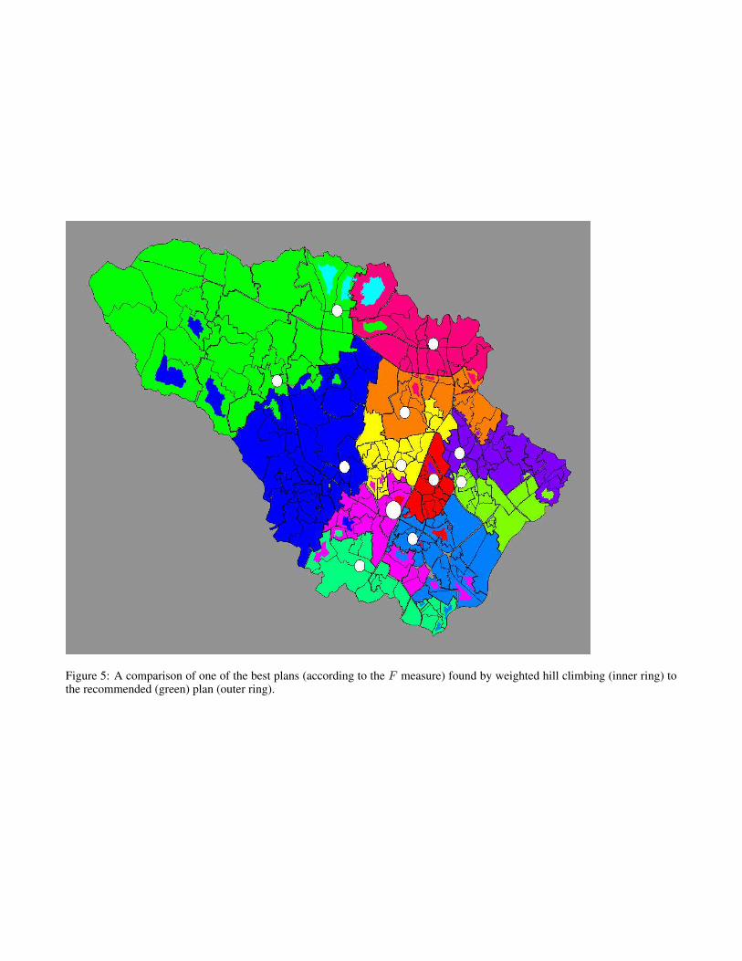
Figure 5: A comparison of one of the best plans (according to the F measure) found by weighted hill climbing (inner ring) tothe recommended (green) plan (outer ring).

Figure 6: Three-way comparison of plans from a representative run of weighted hill climbing.

ing and analyzing political and school redistricting plans.These packages do not generally provide automated or in-teractive search methods, do not provide visual comparisontechniques such as our “tree-ring” comparison, and do notfacilitate the discovery of qualitatively different plans.

Heldig, Orr, & Roediger (1972) were among the earli-est researchers to discuss computational approaches to po-litical redistricting. The focus of their approach is on geo-graphic criteria (compactness, contiguity, and “preservationof natural and/or political boundaries”) and population bal-ancing, although they also mention the possibility of con-sidering other criteria, such as demographic distributions.Their approach is based on linear programming, minimizingan objective function that is specifically designed to maxi-mize geographic compactness of the districts, subject to apopulation-balancing constraint. Variations of this basic ap-proach form the core of most of the more recent computa-tional approaches to redistricting.

Altman’s (1998) dissertation discusses the objective prin-ciples that should ideally be used in political redistricting,including population equality, compactness, and contiguity.He analyzes the computational complexity of political re-districting, and shows that different measures of geographiccompactness can produce very different plans, supporting

our claim that it is important to generate multiple plans fromdifferent perspectives.

School redistricting differs from political redistricting inseveral important ways. First, although compactness is animportant factor (both for community building and to mini-mize busing costs), it is not as important as in political redis-tricting. Second, the walk usage and feeder issues compli-cate the scenario for school redistricting. Third, redistrictingoccurs more frequently (at least in Howard County) than inmost political districts, and students are greatly affected bythe process. As a result, minimizing the number of studentswho are redistricted is also an important criterion. Finally,the nature of the decision-making process, in which alter-native plans are explicitly compared and contrasted to eachother, raises the desirability of generating multiple plans thatrepresent different tradeoffs.

Although we do not yet address all of these issues in ourwork, we believe that the general optimization frameworkwe have developed, based on local search methods, is moreapplicable than those that are commonly used for politicalredistricting, which typically use specialized optimizationalgorithms that focus primarily on geographic constraints.

The problem of multicriteria optimization (also referredto as “multiobjective” and “multiattribute” optimization) has

Figure 7: Three-way comparison of plans from a representative run of diversity-biased hill climbing

been explored by researchers in artificial intelligence, eco-nomics, and operations research. Keeney and Raiffa (1993)discuss a variety of approaches for combining multiple ob-jectives into a single multiattribute utility function. They fo-cus largely on methods for eliciting a single combined utilityfunction. However, in practice, as Keeney and Raiffa pointout, it is not always easy to create a single utility function.This supports our claim that a key component of a decision-making system for school redistricting is to provide toolsthat help the user to understand the nature of the evaluationcriteria and the tradeoffs among them.

Multiattribute optimization techniques include weight-based optimization (where each criterion is assigned aweight, and a combined objective function is optimized),priority-based optimization (where the most important cri-teria are optimized first), and goal programming (in whichone objective is minimized while constraining the others tobe within a given range). None of these methods are idealfor our application, where the tradeoffs are difficult to priori-tize or quantify. They also do not yield multiple qualitativelydifferent solutions; to our knowledge, this problem has notbeen explicitly addressed.

School redistricting is somewhat analogous to the NP-complete problem of multi-objective graph partitioning (Sel-vakkumaran & Karypis 2006), which attempts to optimizemultiple objectives, each of which can be expressed as a sumof edge weights in a graph. Research on this problem hasprimarily used priority-based and weight-based optimiza-tion. The analogy to graph partitioning breaks down in thecase of some of our criteria (walk usage, demographic distri-bution), and as mentioned above, priority-based and weight-based optimization methods do not help us with our goal offinding multiple qualitatively different solutions.

Future WorkOur future work focuses on four primary areas: usability, thecriteria for plan evaluation, visualization of feeder systemsand gradients, and new methods for multiattribute optimiza-tion.

Usability We have demonstrated the current prototype tothe HCPSS Superintendent’s Office, and received a verypositive response. We plan to use our system to producevisualizations that highlight the tradeoffs made by the alter-

native proposed plans in the 2006-2007 redistricting process.Our goal is to make a web-based version of our tool avail-able to the 2007–2008 redistricting committee for viewing,modifying, and evaluating proposed redistricting plans. Weare also planning a more formal user study.

Plan Evaluation Criteria Additional evaluation criteriathat we have explored include feeder quality, compactness,and robustness to future development.

In a pure feeder system, each elementary school wouldmove as a group to a single middle school, and each mid-dle school would move to a single high school. Because ofgeographic and capacity constraints, a pure feeder systemsis impractical; nonetheless, maintaining “feeds” of reason-able size is an important criterion in the process. We havedeveloped a feeder criterion to add to the set of evaluationcriteria,

In most political redistricting approaches, compactness isone of the key factors—and, in fact, is sometimes the onlyfactor that is considered. In school redistricting, compact-ness is desirable, but not explicitly mentioned in the HCPSSmeasured criteria. Furthermore, compactness is already cap-tured indirectly in the busing cost and walk area criteria.However, we plan to explore whether significantly differentplans are produced if compactness is added as an explicitcriterion.

Finally, one ongoing problem with the redistricting pro-cess is that new developments (and new schools) are contin-ually being built. This results in shifting demographics, andcan mean that today’s best plan may lead to overcrowdingat certain schools in a few years. The county does producepopulation projections, but these are inherently uncertain.Future research includes using these projections to measurethe “robustness” of a plan to future planned development.

Visualization We are currently working on new visual-ization techniques that will show feeds more clearly. Theproblem is a challenging one from a visualization perspec-tive, because showing multiple school regions simultane-ously produces a significant amount of “clutter” and corre-sponding cognitive overload.

Another focus of our visualization research is on gradi-ent displays. The gradient along a boundary between twoschool regions characterizes how the plan would change ifa polygon on one side of the boundary were moved to theother school. If the gradient is positive, then the plan tendsto “pull” the polygons along the boundary towards the firstschool. If it is negative, then the plan tends to “push” thepolygons away from the first school. Each evaluation crite-rion can have its own gradient, so some of the gradients maypull, while others push. Developing effective ways to visual-ize these “tensions” on the plan will give the user insight intohow local changes to the plan would change its evaluation.Supporting these displays will also require novel computa-tional techniques for computing and summarizing gradients.

Multiattribute Optimization We are also exploring dif-ferent methods for multicriteria optimization. We have im-

plemented a simulated annealing approach, which is a com-mon technique for such problems. The preliminary resultsfor this approach are not particularly encouraging. Part ofthe problem is that there are many regions of the searchspace that are quite poor (e.g., plans that create islands ofstudents traveling a large distance). Adding an annealingstep tends to lead to poor plans in this search space unlessthe cooling schedule is extremely slow.

We also plan to implement an evolutionary search ap-proach, and are developing a novel multi-agent approach.This approach builds on recent research in combinatorialauctions in a scenario where each polygon can “bid” onschools to attend.

ConclusionsSchool redistricting is an interesting and challenging prob-lem both computationally and from an application perspec-tive. We have developed a prototype system that uses novelheuristic search and visualization techniques to aid an enduser in generating, evaluating, and comparing alternativeplans. These tools should provide end users with significantinsights into the tradeoffs among alternatives.

The school redistricting problem is closely related to theresource positioning problem of deciding where to buildschools, locate fire or police substations, or position emer-gency response equipment. Our optimization framework,search methods, and visualization tools can all potentiallybe applied to these other application domains.

AcknowledgementsThis work was supported by the National Science Founda-tion (grant #IIS-0414976). We would like to thank DavidDrown, Joel Gallihue, and Larry Weaver of the HowardCounty Public School System’s Superintendent’s Office fortheir support, data, and valuable feedback. Thanks alsoto Poonam Shanbhag, who wrote the original visualizationsoftware, and to Andrew Hunt and Priyang Rathod, who alsoworked on the implementation.

ReferencesAltman, M. 1998. Districting principles and democraticrepresentation. Ph.D. Dissertation, California Institute ofTechnology.Caliper Corporation. 2006. Maptitude for redistricting.http://www.caliper.com/mtredist.htm.desJardins, M., and Wagstaff, K. 2005. DD-PREF: A lan-guage for expressing preferences over sets. In Proceedingsof the Twentieth National Conference on Artificial Intelli-gence (AAAI-05).Heldig, R. E.; Orr, P. K.; and Roediger, R. R. 1972. Politi-cal redistricting by computer. Communications of the ACM15(8):735–741.Keeney, R. L., and Raiffa, H. 1993. Decisions with Mul-tiple Objectives: Preferences and Value Tradeoffs. Cam-bridge University Press.Selvakkumaran, N., and Karypis, G. 2006. Multi-objectivehypergraph partitioning algorithms for cut and maximum

subdomain degree minimization. IEEE Transactions onComputer Aided Design 25(3). Forthcoming.Shanbhag, P.; Rheingans, P.; and desJardins, M. 2005.Temporal visualization of planning polygons for efficientpartitioning of geo-spatial data. In Proceedings of InfoVis2005.