hidden markov models - katie.cs.mtech.edu
TRANSCRIPT

CSCI 446: Artificial Intelligence
Hidden Markov Models
Instructor: Michele Van Dyne[These slides were created by Dan Klein and Pieter Abbeel for CS188 Intro to AI at UC Berkeley. All CS188 materials are available at http://ai.berkeley.edu.]

Today
Hidden Markov Models

Probability Recap
Conditional probability
Product rule
Chain rule
X, Y independent if and only if:
X and Y are conditionally independent given Z if and only if:
Reasoning over Time or Space
Often, we want to reason about a sequence of observations
Speech recognition
Robot localization
User attention
Medical monitoring
Need to introduce time (or space) into our models

Markov Models
Value of X at a given time is called the state
Parameters: called transition probabilities or dynamics, specify how the state evolves over time (also, initial state probabilities)
Stationarity assumption: transition probabilities the same at all times
Same as MDP transition model, but no choice of action
X2X1 X3 X4

Conditional Independence
Basic conditional independence: Past and future independent given the present Each time step only depends on the previous This is called the (first order) Markov property
Note that the chain is just a (growable) BN We can always use generic BN reasoning on it if we
truncate the chain at a fixed length

Example Markov Chain: Weather
States: X = {rain, sun}
rain sun
0.9
0.7
0.3
0.1
Two new ways of representing the same CPT
sun
rain
sun
rain
0.1
0.9
0.7
0.3
Xt-1 Xt P(Xt|Xt-1)
sun sun 0.9
sun rain 0.1
rain sun 0.3
rain rain 0.7
Initial distribution: 1.0 sun
CPT P(Xt | Xt-1):

Example Markov Chain: Weather
Initial distribution: 1.0 sun
What is the probability distribution after one step?
rain sun
0.9
0.7
0.3
0.1
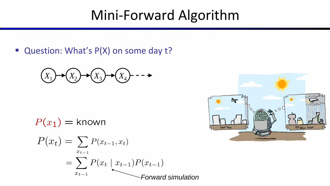
Mini-Forward Algorithm
Question: What’s P(X) on some day t?
Forward simulation
X2X1 X3 X4
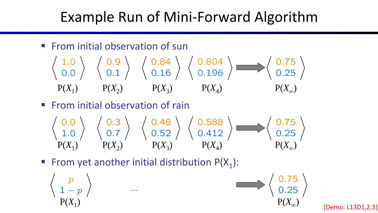
Example Run of Mini-Forward Algorithm
From initial observation of sun
From initial observation of rain
From yet another initial distribution P(X1):
P(X1) P(X2) P(X3) P(X)P(X4)
P(X1) P(X2) P(X3) P(X)P(X4)
P(X1) P(X)
…
[Demo: L13D1,2,3]

Stationary distribution: The distribution we end up with is called
the stationary distribution of the chain
It satisfies
Stationary Distributions
For most chains: Influence of the initial distribution
gets less and less over time.
The distribution we end up in is independent of the initial distribution

Example: Stationary Distributions
Question: What’s P(X) at time t = infinity?
X2X1 X3 X4
Xt-1 Xt P(Xt|Xt-1)
sun sun 0.9
sun rain 0.1
rain sun 0.3
rain rain 0.7
Also:

Application of Stationary Distribution: Web Link Analysis
PageRank over a web graph Each web page is a state
Initial distribution: uniform over pages
Transitions:
With prob. c, uniform jump to arandom page (dotted lines, not all shown)
With prob. 1-c, follow a randomoutlink (solid lines)
Stationary distribution Will spend more time on highly reachable pages E.g. many ways to get to the Acrobat Reader download page Somewhat robust to link spam Google 1.0 returned the set of pages containing all your
keywords in decreasing rank, now all search engines use link analysis along with many other factors (rank actually getting less important over time)
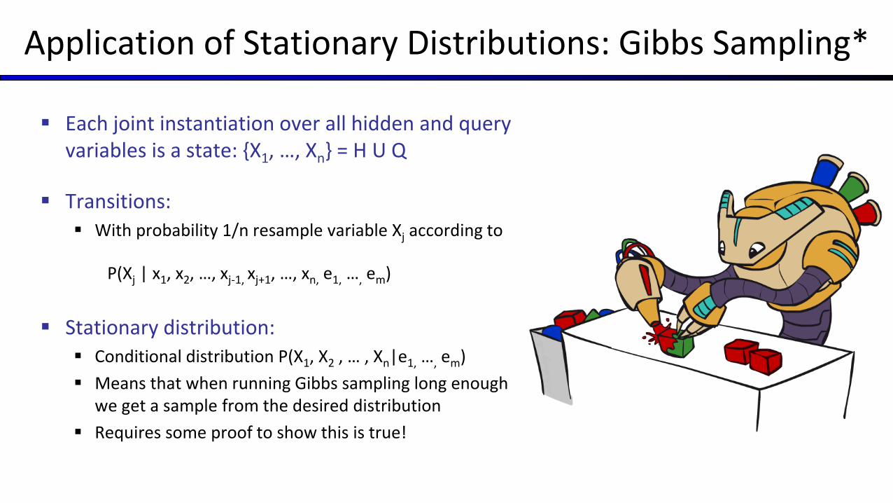
Application of Stationary Distributions: Gibbs Sampling*
Each joint instantiation over all hidden and query variables is a state: {X1, …, Xn} = H U Q
Transitions: With probability 1/n resample variable Xj according to
P(Xj | x1, x2, …, xj-1, xj+1, …, xn, e1, …, em)
Stationary distribution: Conditional distribution P(X1, X2 , … , Xn|e1, …, em)
Means that when running Gibbs sampling long enough we get a sample from the desired distribution
Requires some proof to show this is true!

Hidden Markov Models

Pacman – Sonar (P4)
[Demo: Pacman – Sonar – No Beliefs(L14D1)]
Hidden Markov Models
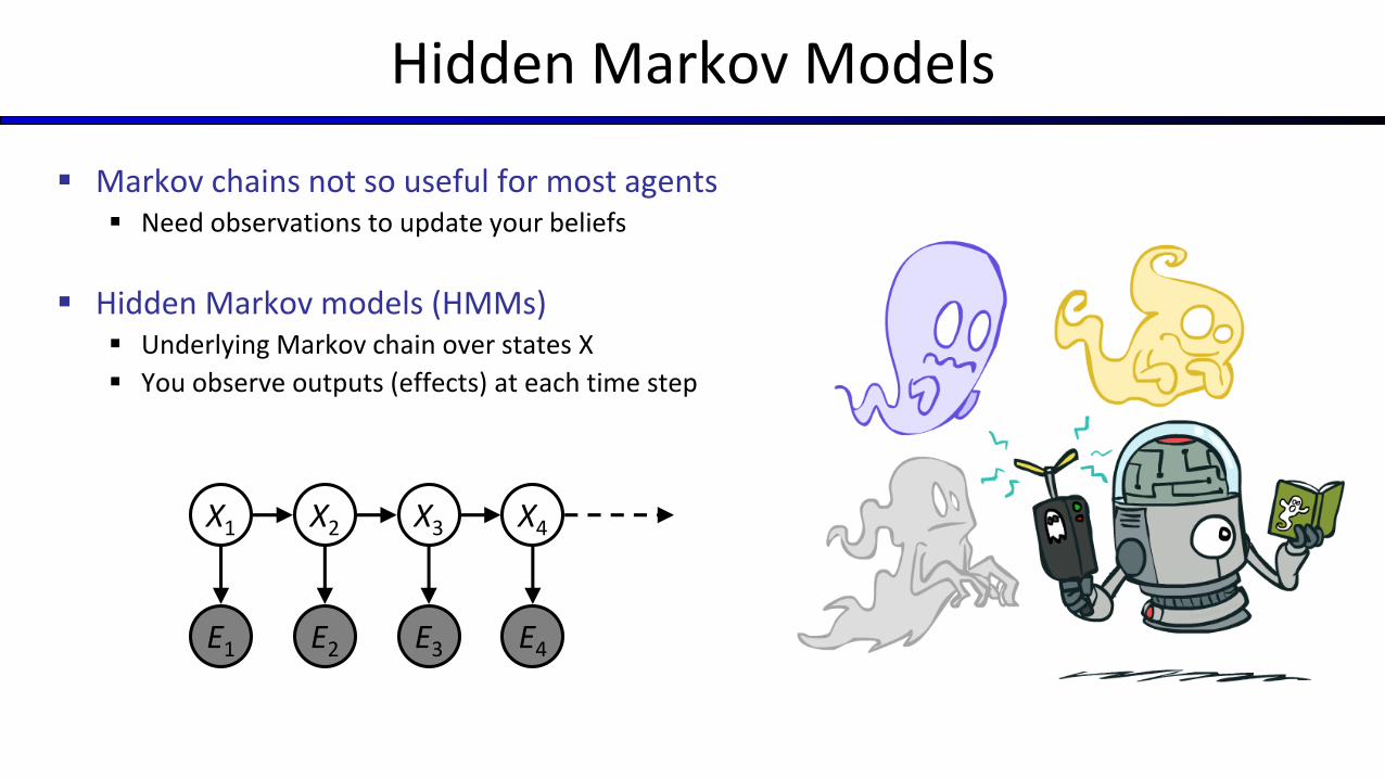
Markov chains not so useful for most agents Need observations to update your beliefs
Hidden Markov models (HMMs) Underlying Markov chain over states X
You observe outputs (effects) at each time step
X5X2
E1
X1 X3 X4
E2 E3 E4 E5

Example: Weather HMM
Rt Rt+1 P(Rt+1|Rt)
+r +r 0.7
+r -r 0.3
-r +r 0.3
-r -r 0.7
Umbrellat-1
Rt Ut P(Ut|Rt)
+r +u 0.9
+r -u 0.1
-r +u 0.2
-r -u 0.8
Umbrellat Umbrellat+1
Raint-1 Raint Raint+1
An HMM is defined by: Initial distribution: Transitions: Emissions:

Example: Ghostbusters HMM
P(X1) = uniform
P(X|X’) = usually move clockwise, but sometimes move in a random direction or stay in place
P(Rij|X) = same sensor model as before:red means close, green means far away.
1/9 1/9
1/9 1/9
1/9
1/9
1/9 1/9 1/9
P(X1)
P(X|X’=<1,2>)
1/6 1/6
0 1/6
1/2
0
0 0 0
X5
X2
Ri,j
X1 X3 X4
Ri,j Ri,j Ri,j
[Demo: Ghostbusters – Circular Dynamics – HMM (L14D2)]

Conditional Independence
HMMs have two important independence properties:
Markov hidden process: future depends on past via the present
Current observation independent of all else given current state
Quiz: does this mean that evidence variables are guaranteed to be independent?
[No, they tend to correlated by the hidden state]
X5X2
E1
X1 X3 X4
E2 E3 E4 E5

Real HMM Examples
Speech recognition HMMs: Observations are acoustic signals (continuous valued)
States are specific positions in specific words (so, tens of thousands)
Machine translation HMMs: Observations are words (tens of thousands)
States are translation options
Robot tracking: Observations are range readings (continuous)
States are positions on a map (continuous)
Filtering / Monitoring
Filtering, or monitoring, is the task of tracking the distribution Bt(X) = Pt(Xt | e1, …, et) (the belief state) over time
We start with B1(X) in an initial setting, usually uniform
As time passes, or we get observations, we update B(X)
The Kalman filter was invented in the 60’s and first implemented as a method of trajectory estimation for the Apollo program
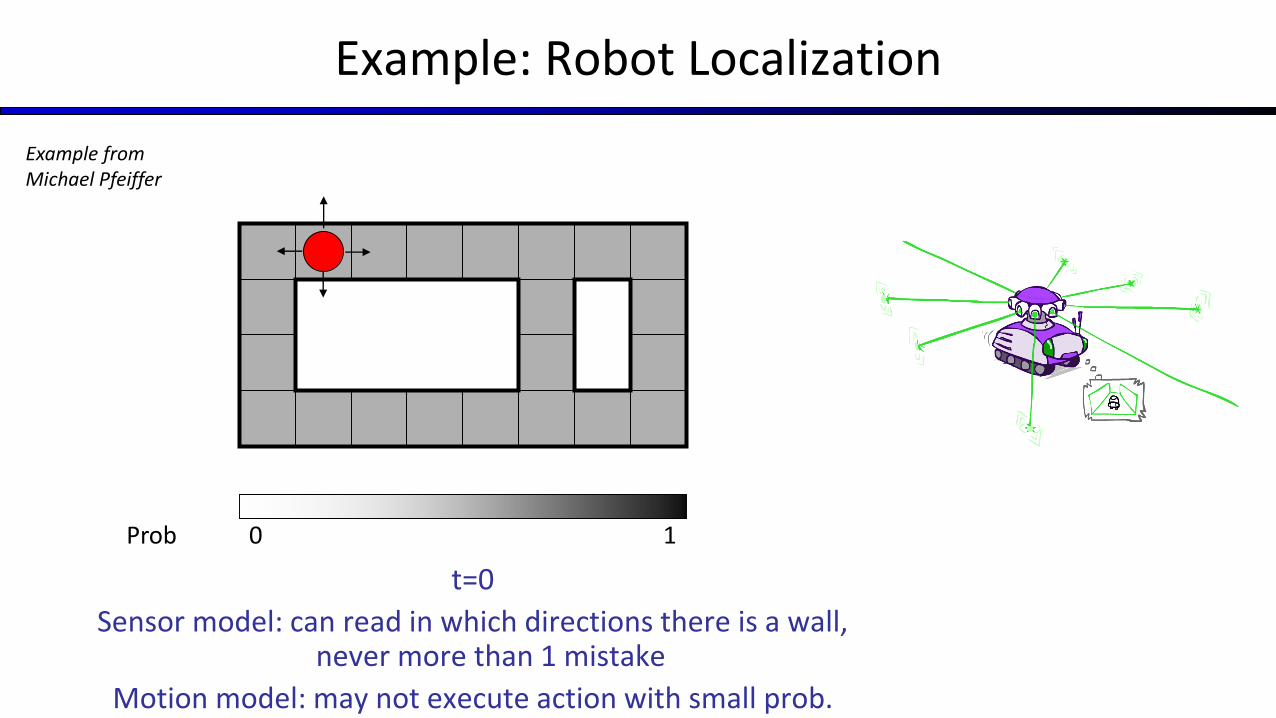
Example: Robot Localization
t=0
Sensor model: can read in which directions there is a wall, never more than 1 mistake
Motion model: may not execute action with small prob.
10Prob
Example from Michael Pfeiffer

Example: Robot Localization
t=1
Lighter grey: was possible to get the reading, but less likely b/c required 1 mistake
10Prob
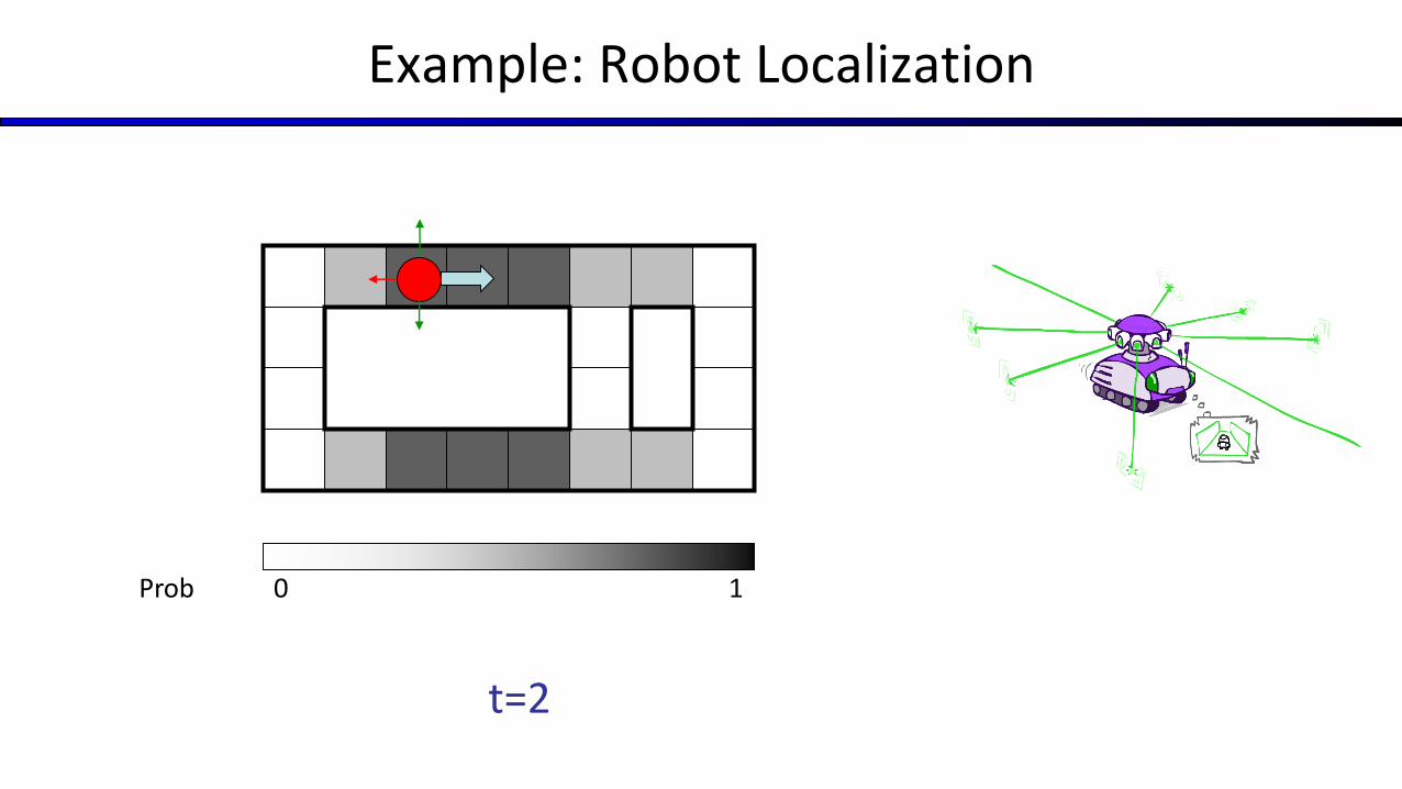
Example: Robot Localization
t=2
10Prob
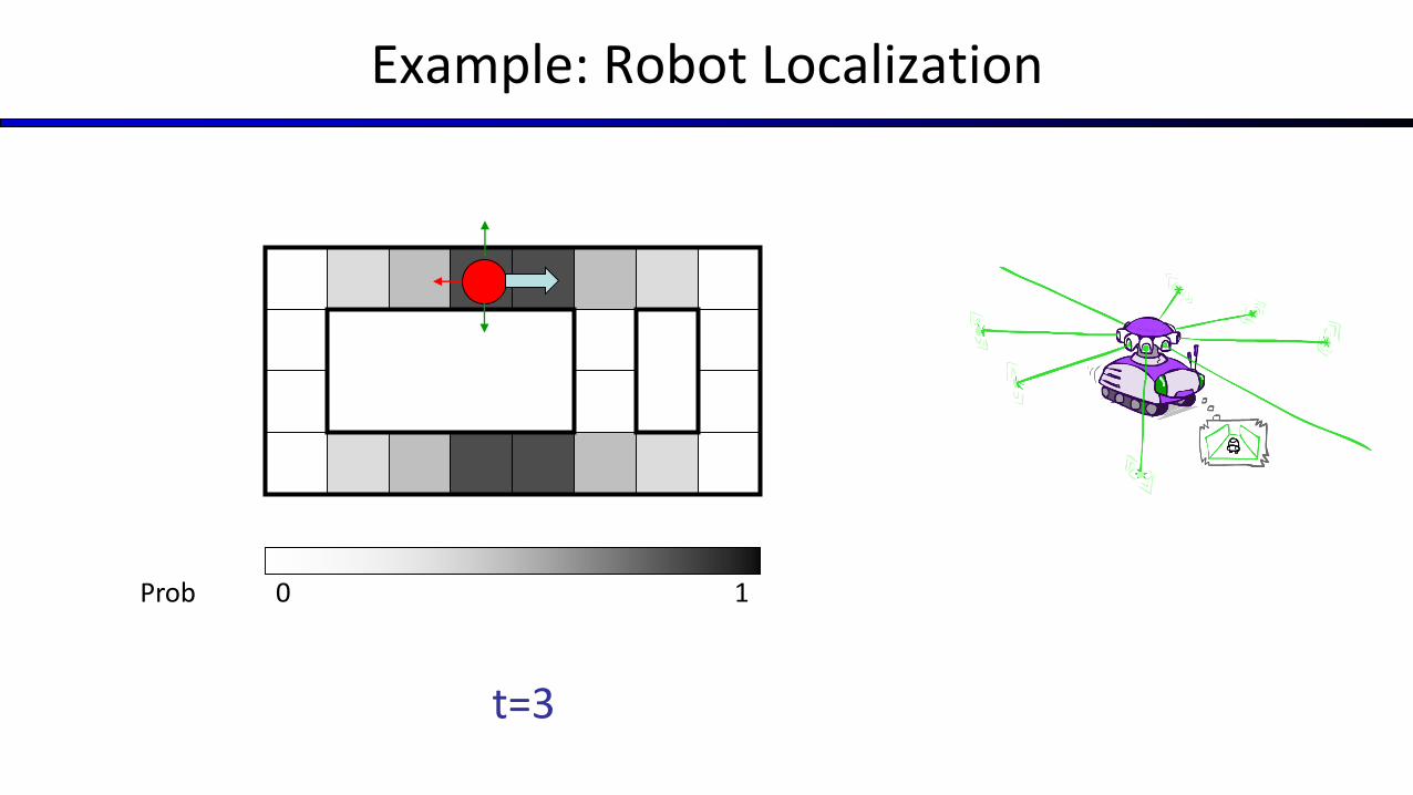
Example: Robot Localization
t=3
10Prob

Example: Robot Localization
t=4
10Prob
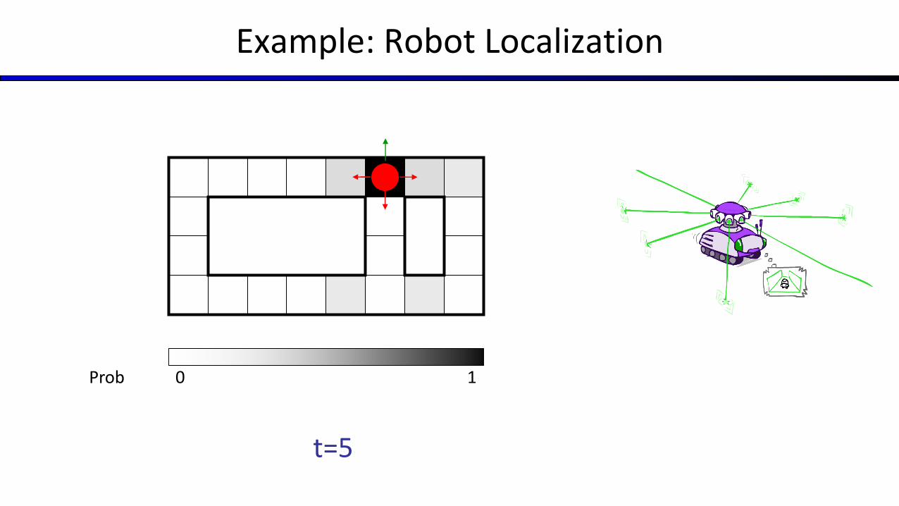
Example: Robot Localization
t=5
10Prob

Inference: Base Cases
E1
X1
X2X1
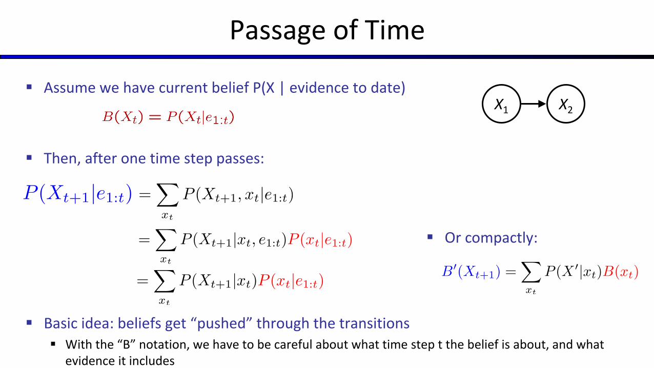
Passage of Time
Assume we have current belief P(X | evidence to date)
Then, after one time step passes:
Basic idea: beliefs get “pushed” through the transitions With the “B” notation, we have to be careful about what time step t the belief is about, and what
evidence it includes
X2X1
Or compactly:

Example: Passage of Time
As time passes, uncertainty “accumulates”
T = 1 T = 2 T = 5
(Transition model: ghosts usually go clockwise)

Observation
Assume we have current belief P(X | previous evidence):
Then, after evidence comes in:
Or, compactly:
E1
X1
Basic idea: beliefs “reweighted” by likelihood of evidence
Unlike passage of time, we have to renormalize
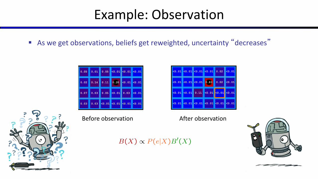
Example: Observation
As we get observations, beliefs get reweighted, uncertainty “decreases”
Before observation After observation

Example: Weather HMM
Rt Rt+1 P(Rt+1|Rt)
+r +r 0.7
+r -r 0.3
-r +r 0.3
-r -r 0.7
Rt Ut P(Ut|Rt)
+r +u 0.9
+r -u 0.1
-r +u 0.2
-r -u 0.8
Umbrella1 Umbrella2
Rain0 Rain1 Rain2
B(+r) = 0.5B(-r) = 0.5
B’(+r) = 0.5B’(-r) = 0.5
B(+r) = 0.818B(-r) = 0.182
B’(+r) = 0.627B’(-r) = 0.373
B(+r) = 0.883B(-r) = 0.117

The Forward Algorithm
We are given evidence at each time and want to know
We can derive the following updatesWe can normalize as we go if we want to have P(x|e) at each time
step, or just once at the end…

Online Belief Updates
Every time step, we start with current P(X | evidence)
We update for time:
We update for evidence:
The forward algorithm does both at once (and doesn’t normalize)
X2X1
X2
E2

Pacman – Sonar (P4)
[Demo: Pacman – Sonar – No Beliefs(L14D1)]

Today
Hidden Markov Models