hiding in plain sight: adversarial neural net facial
TRANSCRIPT

1
Hiding in Plain Sight: Adversarial Neural Net Facial Recognition
Crystal Qian, David Dobkin (Advisor)
Princeton University
{cqian, dpd}@princeton.edu
Abstract
Deep neural networks (DNNs) excel at pattern-recognition tasks, particularly in visual
classification. Implementations of DNN-based facial recognition systems [1, 5, 8] approach and
even exceed human-level performance on certain datasets [2]. However, recent studies [4, 6, 8]
have revealed that imperceptible image perturbations can result in object misclassification in
neural network-based systems. We explore the effects of image-agnostic perturbation methods at
various stages of the facial recognition pipeline on network prediction errors, specifically training
perturbations of the widely-used Labeled Faces in the Wild (LFW) dataset on FaceNet.
1. Introduction
Deep neural networks are widely
implemented in facial recognition systems
due to their excellent performance in visual
classification. However, these networks do
exhibit certain counterintuitive defects; for
example, applying imperceptible non-
random perturbations to images can
arbitrarily change the network’s prediction
[8]. That is, because neurons in the network
are activated on a linear combination of
inputs, slight changes to the input accumulate
in large changes to the output. These
perturbations cause misclassifications across
varied neural network-based systems, so we
know that the intrinsic “blind spots” exist
within the neural networks themselves [8].
In this paper, we present results on neural
network object misclassification specifically
focused on facial recognition systems and the
Labeled Faces in the Wild (LFW) dataset. To
that end, we experiment with perturbations
along the alignment, representation, and
classification steps of the generally accepted
facial recognition pipeline.
Additionally, our results focus on the effects
of random perturbations rather than non-
random perturbations; in other words, noise.
We convolute images at varying levels of
noise with Gaussian and Poisson noise
distributions. The visual results are not
imperceptible, but recognizable to varying
degrees.
Research in this space has demonstrated the
effects of non-random perturbations through
the generation of adversarial examples.
While these examples yield higher
misclassification rates relative to the degree
of convolution, it is important to study the
effects of image-agnostic convolution to, at
the least, present a more robust baseline than
is currently available.

2
2. Previous work
Labeled Faces in the Wild (LFW) is a
database of 5,749 labelled people spanning
13,233 images. Most facial recognition
systems test accuracy on this database as a
benchmark; supervised recognition systems
far exceed the performance of traditional
recognition systems.
System Accuracy Supervised
Eigenfaces 0.6000 No
Fisherfaces 0.8747 No
DeepFace 0.9725 Yes
Human vision 0.9750 -
FaceNet 0.9963 Yes Table 1: Accuracy of recognition systems on the
LFW dataset [2, 5, 9].
Additionally, certain flaws have been
exposed in neural network recognition
systems, leading to misclassification of
objects. Generally, imperceptible changes in
an image should not alter the classification.
However, smoothness assumptions that
underlie certain kernel methods do not
necessarily hold for neural networks.
Szegedy et. produced the following objective
of applying a perturbation r to an input x (classified as f(x) by a deep neural network):
argmin𝑟 (|𝑓(𝑥 + 𝑟) − ℎ𝑡| + 𝜅|𝑟|
𝑥 + 𝑟 ∈ [0, 1], 𝑓 produces a probability
distribution over possible classes, 𝜅 is a
constant and ℎ𝑡 is a one-hot vector of an
arbitrary class (the class is encoded as a
vector of booleans, with 1 or 0 indicating the
presence of a characteristic). Minimizing
|𝑓(𝑥 + 𝑟) − ℎ𝑡| results in misclassification,
and minimizing 𝜅|𝑟| increases
imperceptibility [7]. To generate
imperceptible perturbations that serve as
adversarial examples for recognition
systems, we optimize this function.
The ability to generate these adversarial
examples is a “blind spot” in neural network-
based recognition systems because these
examples are improbable to encounter in
training when learning from finite training
sets; the non-flexibility of classification
models further encourages this result [8].
Thus far, the effects of these non-random
perturbations have been studied on object
classification datasets like MNIST and
ImageNet, but not so much on facial
recognition datasets. Sharif et. al generated
adversarial examples for a small sample of
faces (DNN𝐵 trained on 10 subjects and
DNN𝐶trained on 143), but largely focused on
physically realizable disguises to counter
facial recognition systems.
Most studies have generated adversarial
examples through non-random perturbation.
Szedezy et. al does observe the effects of
Gaussian noise (with stddev = 1) as a baseline
on the MNIST dataset as a baseline; the
results are vaguely recognizable and resulted
in 51% accuracy of classification.
Though the results on MNIST were visually
perceptible, we should study the effects of
noise on recognition systems as well; at the
least, to provide a baseline for future studies
in generating adversarial examples for neural
network-based facial recognition. Can
random noise significantly decrease the
accuracy rate of various neural networks with
minimal perturbation? Do networks trained
on different classifiers respond similarly to
perturbation? Do all types of noise: additive,
multiplicative, applicative, etc. applied in the
same amount result in the same degree of
accuracy?

3
3. Methodology
We chose FaceNet (and the OpenFace/
OpenCV implementation) as our recognition
system because of its strong performance on
the LFW dataset (99.63% accuracy). Our
LFW dataset is condensed to 6,715 images of
610 people instead of 13,233 images of 5,759
people, filtered so that all people in our
dataset have at least 4 images for cross-
validation. Our experiments target most
stages of the recognition pipeline [9].
1. Detection
2. Alignment
3. Classification
4. Representation
Detection isn’t altered because all images in
LFW are guaranteed to be of labelled faces.
3.1 Alignment
We align faces by the outer eyes and nose,
and by the inner eyes and bottom lip. Does
alignment affect classification accuracy?
Figure 1: Andre_Agassi_007.jpg. Left: outer
eyes and nose alignment. Right: inner eyes and
bottom lip alignment.
3.2 Classification
We classify faces using the following models
and parameters.
- A support vector machine with linear
kernel (linear SVM).
- A support vector machine with radial
basis function kernel (radial SVM)
and 𝛾 = 2.
- A decision tree classifier with
maximum depth = 20.
- Gaussian Naïve Bayes, taking in
LFW as a training set.
- A deep belief network (DBN) with a
learning rate decay of .9, learning rate
of .3, and 300 epochs.
Does the classifier used in training the neural
network affect response to perturbation? Are
different types of classifiers sensitive to
certain types or degrees of noise?
3.3 Representation
We mainly apply noise in an additive
Gaussian distribution, with 𝜎2 = 16, 𝜎2 =
100, 𝜎2 = 500, and 𝜎2 = 1000. We also
test the effects of Poisson noise (applied
noise). Do different types of noise, applied in
the same degree, affect classification
accuracy to the same extent?
Parameters for Gaussian noise’s 𝜎 were
determined at intervals where the differences
in perceptibility could easily be identified.
Figure 2: George_Clooney_0005.jpg. Top left:
original image. Top middle: 𝜎2 = 16. Top right:
𝜎2 = 100. Bottom left: 𝜎2 = 500. Bottom right:
𝜎2 = 1000.

4
Figure 3: Adam_Sandler_0001.jpg. Top left:
original image. Top middle: 𝜎2 = 16. Top right:
𝜎2 = 100. Bottom left: 𝜎2 = 500. Bottom right:
𝜎2 = 1000.
With 𝜇 is as mean pixel value and 𝜎 as the
standard deviation, the additive Gaussian
distribution is calculated as follows:
𝑓(𝑧) = 1
𝜎√2𝜋𝑒
−(𝑧−𝜇)2
2𝜎2
Noise for the Poisson distribution is
calculated with the following:
𝑓(𝑘, 𝜆) = 𝜆𝑘𝑒−𝜆
𝑘!
Where 𝑘 = 1 and 𝜆 is sampled from the
image, taking in factors such as the number
of unique pixels.
We test this Poisson noise against Gaussian
noise 𝜎2 = 16, which has the same amount of
perturbation (summed absolute value of all
changes made to each pixel).
Figure 4: Britney_Spears_0001.jpg. Left:
original image. Middle: image with Poisson
noise. Right: image with Gaussian noise, 𝜎2 =
16.
3.4 Implementation
The code used is written in a mix of Python,
Lua, and Bash scripts, and is largely reliant
on OpenFace and scikit. This is available at
github.com/cjqian/facetraining.
4. Experimentation and results
Here are the parameters we alter at different stages of the recognition pipeline: alignment,
representation, classification.
Alignment Methods Noise Generators Classification Systems
Outer eyes and nose Poisson Linear SVM
Inner eyes and bottom lip Gaussian, 𝜎2 = 16 Radial SVM, 𝛾 = 2
Gaussian, 𝜎2 = 100 Decision Tree
Gaussian, 𝜎2 = 500 Gaussian Naive Bayes
Gaussian, 𝜎2 = 1000 Deep Belief Network
Table 2: Summary of experiment parameters.

5
4.1 Metrics
We use individual and comparative metrics on each experiment (tests run on one alignment
method, one noise generator and one classification system) for evaluation.
Individual: We use the following individual metrics. A detected ratio is the number of faces
detected out of the total number of faces in the dataset (in our case, 6715). A recognized ratio is
the number of recognized faces (correctly identified labels) out of detected faces.
Metric Value Value
Probability
Detected 5425/6715 .807
Recognized 3503/5425 .645
Table 3: Individual metrics for inner aligned
dataset, no noise generated and linear SVM.
Metric Value Value
Probability
Detected 5152/6715 .767
Recognized 3266/5152 .633
Table 4: Individual metrics for inner aligned
dataset, Gaussian noise with 𝜎2 = 100 and linear
SVM.
With no noise, here are some examples of misclassification using inner alignment.
Figure 5: Left: Pamela_Anderson_0003
misclassified as Angelina Jolie with .029 confidence.
Right: Angelina_Jolie_0006.
Figure 6: Left: Queen_Latifah_0004
misclassified as Condoleezza Rice with .013
confidence. Right: Condoleezza_Rice_0001.
Comparative: We test experiments with generated noise (altered) against the same experiments
with no generated noise (baseline) using the following comparative metrics:
- The lost count: faces detected in the baseline but not detected in the altered experiment.
- The found count: faces not detected in the baseline but detected in the altered experiment.
- The disguised count: faces were correctly classified in the baseline but misclassified or not
detected in the altered experiment.
- The exposed count: faces not correctly identified or not detected in the baseline but
correctly classified in the altered experiment.
Metric Value
Lost 409
Found 136
Disguised 454
Exposed 217
Improved 1266/3049 (.412)
Improved score 12.96
Table 5: Comparative metrics for inner aligned
dataset, Gaussian noise with 𝜎2 = 100 and
linear SVM.
Metric Value
Lost 4151
Found 17
Disguised 2896
Exposed 25
Improved 108/607 (.1779)
Improved score 50.69
Table 6: Comparative metrics for inner aligned
dataset, Gaussian noise with 𝜎2 = 1000 and
linear SVM.

6
Here are examples of disguised or exposed faces after applying Gaussian noise at 𝜎2 = 100.
Figure 7: Left: Vladimir_Putin_0032 with .097
confidence (no noise). Right: Silvio Berlusconi with
.071 confidence. Disguised.
Figure 8: Left: Christina_Aguilera_0003
identified as Anna Kournikova with .014
confidence (no noise). Right: Correctly identified
Christina Aguilera with .012 confidence. Exposed.
4.2 Alignment Results
Detection: All classification systems detected the same number of faces per noise type within their
alignment. Images aligned by the inner eyes and bottom lip consistently detected more faces than
in images aligned by the outer eyes and nose. The graph below shows these results; we computed
the net faces detected by subtracting the number of faces exposed from the number of faces
disguised.
Recognition: Although the type of classification system in use did affect the number of faces
recognized, inner aligned faces were more correctly classified in most cases. The ratio of faces
detected to recognized stays approximately the same for the two alignment methods across
classification systems, indicating that although alignment by the inner eyes and bottom lip cause
more faces to be detected (and subsequently correctly classified), differing alignment methods do
not affect the classification accuracy.
0
1000
2000
3000
4000
5000
6000
None Poisson Gaussian, σ^2=16 Gaussian, σ^2=100 Gaussian, σ^2=500 Gaussian, σ^2=1000
Net fa
ces d
ete
cte
d
Noise type
Figure 9: Net detected faces
Inner alignment Outer alignment

7
Here are some results with the two alignments and no noise. We use the linear SVM classifier.
Figure 11: Colin_Powell_0071. Left: outer alignment,
no face detected. Right: inner alignment, no face
detected.
Figure 12: Colin_Powell_0207. Left:
outer alignment, face detected and
correctly classified with .621 confidence.
Right: inner alignment, face detected and
correctly classified with .806 confidence.
Figure 13: Anna_Kournikova_0004. Left: outer
alignment, face detected but misclassified as Arnold
Schwarzenegger with .016 confidence. Right: inner
alignment, face detected and correctly classified with
confidence .015.
Figure 14: Michelle_Yeoh_0003. Left: outer
alignment, no face detected. Right: face
detected but misclassified as Anna
Kournikova with .0139 confidence.
Moving forward, we’ll mainly use results of inner alignment, since we’ve show that
classification accuracy of varying perturbations is consistent across alignments.
0
0.1
0.2
0.3
0.4
0.5
0.6
0.7
0.8
None Poisson Gaussian, σ^2=16 Gaussian, σ^2=100 Gaussian, σ^2=500 Gaussian, σ^2=1000Ratio o
f fa
ces r
ecogn
ized/d
ete
cte
d
Noise Type
Figure 10: Percentage of detected faces that are recognized on linear SVM data
Inner alignment Outer alignment

8
4.3 Classifier Results
We decided to test primarily the effects of Gaussian (additive) noise. To calculate net faces
disguised across different classifiers along different values for 𝜎2, we subtract the number of
faces exposed from the number of faces disguised. For each classifier, the results fit a quadratic
trendline nicely with minimal 𝑟2 = .998.
This indicates that the number of faces disguised scales linearly with the amount of perturbation
added to the image.
Here are the classifiers in ascending order by number of faces disguised. The numbers are in dark
green if more faces were disguised than revealed, and red if the opposite is true. Notice that for
𝜎2 = 16, perturbing the faces improve the detection rate slightly. (Discussed more in 4.3). “D” is
short for “Disguised,” “R” is short for “Revealed,” and “T” is the total number of faces recognized.
𝜎2 = 16 𝜎2 = 100 𝜎2 = 500 𝜎2 = 10𝟎𝟎
D R T D R T D R T D R T
Decision Tree 287 304 1664 340 234 1513 863 135 739 1134 56 250
Linear SVM 325 440 4612 454 217 4281 1862 94 2112 2896 25 722
Radial SVM 285 288 3618 628 300 3266 2604 107 1735 3916 29 632
Gaussian Naïve Bayes 261 272 4830 585 284 4518 2597 119 2341 4057 29 791
DBN 278 260 4911 585 268 4612 2648 118 2399 4100 30 859
Table 7: Number of faces disguised v. revealed for inner aligned data.
To check if certain types of classifiers are more susceptible to misclassification, we normalize
the net disguise value found in table X and divide by the “quality of recognition,” calculated by
dividing T over the total number of faces recognized at 𝜎2 = 0, or at no perturbed noise.
-500
0
500
1000
1500
2000
2500
3000
3500
4000
4500
0 200 400 600 800 1000 1200
Net fa
ces d
isgu
ised
𝜎^2
Figure 15: Net disguised values
Linear SVM
Radial SVM
Decision Tree
Gaussian Naïve Bayes
DBN
Poly. (Linear SVM)
Poly. (Radial SVM)
Poly. (Decision Tree)
Poly. (Gaussian Naïve Bayes)
Poly. (DBN)

9
All the trendlines fit along a quadratic curve with minimum correlation = .995, and the lines are
mostly similar (with the exception of linear SVM). The similarities in the trendlines indicate that
the classification systems are equally susceptible to perturbations.
Here are some case studies showing the results of classification on single faces. Notice the
unexpected variance of confidence values along classifiers.
𝜎2 = 0 𝜎2 = 16 𝜎2 = 100 𝜎2 = 500 𝜎2 = 10𝟎𝟎
Decision Tree
Classified with 1.0
confidence.
Classified with 1.0
confidence.
Classified with 1.0
confidence.
Misclassified as
Jackie Chan with .056 confidence.
Misclassified as
Jackie Chan with .056 confidence.
Linear SVM Classified with .087
confidence.
Classified with .073
confidence.
Classified with .076
confidence.
Classified with .054
confidence Classified with .026
confidence Radial SVM Classified with .069
confidence. Classified with .065 confidence.
Classified with .068 confidence.
Misclassified as Junichiro Koizumi with .0316 confidence.
Misclassified as Junichiro Koizumi with .0226 confidence.
Gaussian Naïve Bayes
Classified with 1.0
confidence.
Classified with 1.0
confidence.
Classified with 1.0
confidence.
Classified with .999
confidence.
Misclassified as
Tung Chee-hwa with .515 confidence.
DBN Classified with .939
confidence.
Classified with .923
confidence.
Classified with .973
confidence.
Classified with .756
confidence. Classified with .362
confidence. Table 8: Case study of Roh_Moo-hyun_0004.
0
0.2
0.4
0.6
0.8
1
1.2
0 200 400 600 800 1000 1200
Norm
aliz
ed r
ecogn
itio
n s
core
𝜎^2
Figure 16: Normalized disguised values
Decision Tree
Radial SVM
Linear SVM
Gaussian Naïve Bayes
DBN
Poly. (Decision Tree)
Poly. (Radial SVM)
Poly. (Linear SVM)
Poly. (Gaussian Naïve Bayes)
Poly. (DBN)

10
𝜎2 = 0 𝜎2 = 16 𝜎2 = 100 𝜎2 = 500 𝜎2 = 10𝟎𝟎
Decision Tree
Misclassified as Vladimir Putin with .016 confidence.
Misclassified as Vladimir Putin with .016 confidence.
Misclassified as Michael Douglas with .033 confidence.
Misclassified as Michael Douglas with .033 confidence.
Misclassified as Michael Douglas with .033 confidence.
Linear SVM Misclassified as
Paul Bremer with .028 confidence.
Misclassified as
Paul Bremer with .024 confidence.
Misclassified as
Paul Bremer with .0316 confidence.
Misclassified as
Paul Bremer with .043 confidence.
Misclassified as
Paul Bremer with .035 confidence.
Radial SVM Classified with .024 confidence.
Classified with .024 confidence.
Classified with .027 confidence.
Classified with .029 confidence.
Classified with .024 confidence.
Gaussian Naïve Bayes
Classified with 1.0
confidence.
Classified with 1.0
confidence.
Classified with 1.0
confidence.
Classified with 1.0
confidence. Classified with 1.0
confidence.
DBN Classified with
.925 confidence.
Classified with
.907 confidence.
Classified with
.755 confidence.
Classified with .831
confidence. Classified with
.854 confidence. Table 9: Case study of Joan_Laporta_0008.
Each classifier’s relationship with the perturbations is not intuitive. Glaring inconsistencies, like
how confidences can increase with added perturbation or how faces can be revealed with added
perturbation, reaffirm that deep neural networks learned by back propagation “have nonintuitive
characteristics and intrinsic blind spots, whose structure is connected to the data distribution in a
non-obvious way” [8].
4.4 Noise Generation Results (Poisson v. Gaussian)
Intuitively, adding random noise to a face should lower the number of recognized faces across our
dataset for all classification systems. This assumption is consistent with the results that we’ve seen
for perceptible amounts of random Gaussian noise.
However, for nearly imperceptible amounts of noise (Poisson noise, Gaussian with 𝜎2 = 16), there
is a net increase in exposed faces in evaluating the classifications from each individual experiment.
-40 -20 0 20 40 60 80 100 120 140
Decision Tree
Radial SVM
Linear SVM
Gaussian Naïve Bayes
DBN
Difference from baseline's recognized value
Figure 17: Difference in recognition values from baseline
Gaussian Poisson

11
This irregularity is further indicated when comparing the net disguised value (number of disguised
faces – number of exposed faces) across classifiers. For perceptible Gaussian noise perturbations,
this value is consistently positive. For small perturbations, more faces are exposed by perturbation
than are disguised, leading to a negative net disguised value.
Additionally, the small Gaussian and Poisson perturbations contribute roughly the same amount
of noise in the face. However, the Gaussian noise does a statistically significant worse job at
disguising faces than the Poisson noise.
4.5 Other Results
Raw data used for analysis can be found in the appendix. Also, files, code, and log files can be
found here: github.com/cjqian/facetraining. This includes specific lists for each experiment
indicating which images where disguised, exposed, lost, etc.
For individual metrics, we also computed a confidence score. If a face was correctly classified
with n confidence, we add n to the score. If a face was misclassified with m confidence, we subtract
m from the score. At a glance, this confidence score seems loosely related to the
recognized/detected ratio.
For comparative metrics, we compute an additional improve value and corresponding score. If a
face is correctly classified in both the baseline and additional experiment, it is considered improved
if the confidence value is higher in the additional experiment. The score sums the degree to which
this improvement is made. A disguise is considered more successful if the improve ratio is small.
-140 -120 -100 -80 -60 -40 -20 0 20 40
Decision Tree
Radial SVM
Linear SVM
Gaussian Naïve Bayes
DBN
Figure 18: Net disguised values
Gaussian Poisson

12
5. Conclusions
We altered parameters at various stages of the
recognition pipeline (see Table 2) to test how
the perturbation of faces affects
classification.
Alignment: Aligning faces by the inner eyes
and bottom lip result in higher detection and
recognition accuracy than aligning faces by
the outer eyes and nose. This result is
consistent across the five classifiers tested.
However, the ratio of faces disguised across
varying perturbations over the total amount
of faces classified is approximately the same
for either alignment method, indicating that
alignment plays no apparent role in
disguising faces.
Representation: The more perceptible
(significant) noise is added to our dataset, the
more faces are misclassified. However, the
relationship between these changes is
relatively inconsistent on an individual basis;
adding noise can increase confidence or
expose faces in many cases. Furthermore,
adding small amounts of noise exposes more
faces overall, even to a statistically
significant amount in the case of certain
classifiers.
Classification: Neural networks trained with
different classifiers result in different
detection and recognition accuracies. In order
from highest accuracy to lowest on our
dataset:
1. DBN
2. Gaussian Naïve Bayes
3. Radial SVM
4. Linear SVM
5. Decision Trees
Refer to Table 7 for more detail. Although
the disguised accuracies varied across
classifiers, these accuracy scores normalized
(by dividing against each classifier’s
recognition accuracies) showed that these
classifiers responded similarly to
perturbations.
In summary, alignment and classification
method do not noticeably alter the effects of
perturbation on the LFW dataset, showing
that the classification abilities of neural
networks are consistent across classification
methods and the skewing of images in our
dataset. However, these perturbations are
proven to alter the classifications in
unintuitive ways.
6. Future Work
The unintuitive classifications should be
explored in much greater detail.
Why does adding small amounts of noise
increase the exposure of faces across
classifiers? To verify that this is a consistent
result, we should test on other datasets and
recognition systems aside from FaceNet.
Why does the Gaussian noise distribution do
a worse job at disguising faces than the
Poisson noise distribution in most cases,
despite contributing overall the same amount
of change? Expanding the study to include
more types of additive, multiplicative, and
applied noise to similar degrees can indicate
if the type of noise plays a more significant
role in disguising faces.
Can we gain an intuition for how
misclassification occurs in neural networks-
based recognition systems? The results of our
experiments reveal inconsistencies; faces that
are not detected or recognized should not
become exposed by adding random noise as
they are currently. Which layers of DNNs or
features of these classifiers cause the
unpredictable confidence score changes and
classifications?
13
6. Honor Statement
I pledge my honor that this paper represents my own work in accordance with University
regulations.
7. References
[1] Amos, Brandon, Bartosz Ludwiczuk, and Mahadev Satyanarayanan. OpenFace: A
general-purpose face recognition library with mobile applications. Technical report,
CMU-CS-16-118, CMU School of Computer Science, 2016.
[2] Huang, Gary B., et al. Labeled faces in the wild: A database for studying face recognition
in unconstrained environments. Vol. 1. No. 2. Technical Report 07-49, University of
Massachusetts, Amherst. 2007.
[3] Goodfellow, Ian J., Jonathon Shlens, and Christian Szegedy. "Explaining and harnessing
adversarial examples." arXiv preprint arXiv:1412.6572. 2014.
[4] Nguyen, Anh, Jason Yosinski, and Jeff Clune. "Deep neural networks are easily fooled:
High confidence predictions for unrecognizable images." 2015 IEEE Conference on
Computer Vision and Pattern Recognition (CVPR). IEEE, 2015.
[5] Schroff, Florian, Dmitry Kalenichenko, and James Philbin. "Facenet: A unified
embedding for face recognition and clustering." Proceedings of the IEEE Conference on
Computer Vision and Pattern Recognition. 2015.
[6] Seyed-Mohsen, Moosavi-Dezfooli, Alhussein Fawzi, Omar Fawzi, and Pascal Frossard.
“Universal adversarial perturbations.” CoRR abs/1610.08401. 2016.
[7] Sharif, Mahmood, et al. "Accessorize to a crime: Real and stealthy attacks on state-of-
the-art face recognition." Proceedings of the 2016 ACM SIGSAC Conference on
Computer and Communications Security. ACM, 2016.
[8] Szegedy, Christian, et al. "Intriguing properties of neural networks." arXiv preprint
arXiv:1312.6199 (2013). Sharif, Mahmood, et al. "Accessorize to a crime: Real and
stealthy attacks on state-of-the-art face recognition." Proceedings of the 2016 ACM
SIGSAC Conference on Computer and Communications Security. ACM, 2016.
[9] Taigman, Yaniv, et al. "Deepface: Closing the gap to human-level performance in face
verification." Proceedings of the IEEE Conference on Computer Vision and Pattern
Recognition. 2014.

8. Appendix
The following data is for inner alignment experiments, since we use these for the majority of
results in this paper. Refer to 4.5 for additional information or data.
8.1. Output files
Linear SVM:
None Poisson Gaussian
𝜎2 = 16
Gaussian
𝜎2 = 100
Gaussian
𝜎2 = 500
Gaussian
𝜎2 = 1000
Detected Value 5425 5428 5409 5152 3104 1291
Detected Ratio* .807 .808 .805 .767 .462 .192
Recognized Value 3503 3508 3618 3266 1735 632
Recognized Ratio** .645 .646 .668 .633 .558 .489
Confidence 698.2 697.4 677.6 657.0 335.6 113.6
Table 10: Individual metrics.
Poisson Gaussian
𝜎2 = 16
Gaussian
𝜎2 = 100
Gaussian
𝜎2 = 500
Gaussian
𝜎2 = 1000
Lost 123 140 409 2372 4151
Found 126 124 136 51 17
Disguised 190 325 454 1862 2896
Exposed 195 440 217 94 25
Improved 1617/3313 1535/3178 1266/3049 399/1641 108/607
Improved ratio .488 .483 .415 .243 .175
Improved score -1.41 29.20 12.96 82.34 .369
Table 11: Comparative metrics.
Radial SVM:
None Poisson Gaussian
𝜎2 = 16
Gaussian
𝜎2 = 100
Gaussian
𝜎2 = 500
Gaussian
𝜎2 = 1000
Detected Value 5425 5428 5409 5152 3104 1291
Detected Ratio .807 .808 .805 .767 .462 .192
Recognized Value 4609 4602 4612 4281 2112 722
Recognized Ratio .849 .847 .852 .830 .558 .559
Confidence 684.3 687.2 689.9 647.1 328.5 105.6
Table 12: Individual metrics.
Poisson Gaussian
𝜎2 = 16
Gaussian
𝜎2 = 100
Gaussian
𝜎2 = 500
Gaussian
𝜎2 = 1000
Lost 123 140 409 2372 4151
Found 126 124 136 51 17
Disguised 290 285 628 2604 3916
Exposed 283 288 300 107 29
Improved 2181/4319 2171/4324 1780/3981 553/2005 132/693
Improved ratio .505 .502 .447 .275 .190
Improved score -4.01 -4.92 6.05 73.26 51.76
Table 13: Comparative metrics.

Decision Tree:
None Poisson Gaussian
𝜎2 = 16
Gaussian
𝜎2 = 100
Gaussian
𝜎2 = 500
Gaussian
𝜎2 = 1000
Detected Value 5425 5428 5409 5152 3104 1291
Detected Ratio .807 .808 .805 .767 .462 .192
Recognized Value 1647 1651 1664 1513 739 250
Recognized Ratio .303 .304 .307 .293 .238 .193
Confidence 513.1 483.4 523.3 385.0 -59.3 483.4
Table 14: Individual metrics.
Poisson Gaussian
𝜎2 = 16
Gaussian
𝜎2 = 100
Gaussian
𝜎2 = 500
Gaussian
𝜎2 = 1000
Lost 123 140 409 2372 4151
Found 126 124 136 51 17
Disguised 289 287 466 1096 1441
Exposed 293 304 332 188 50
Improved 4/1358 4/1360 9/1181 4/551 0/200
Improved ratio .003 .003 .008 .007 0
Improved score 1.463 2.847 .417 6.01 1.141
Table 15: Comparative metrics.
Gaussian Naïve Bayes:
None Poisson Gaussian
𝜎2 = 16
Gaussian
𝜎2 = 100
Gaussian
𝜎2 = 500
Gaussian
𝜎2 = 1000
Detected Value 5425 5428 5409 5152 3104 1291
Detected Ratio .807 .808 .805 .767 .462 .192
Recognized Value 4819 4832 4830 4518 2341 791
Recognized Ratio .888 .890 .892 .876 .754 .612
Confidence 4229 4244 4261 3899 1600 306.4
Table 16: Individual metrics.
Poisson Gaussian
𝜎2 = 16
Gaussian
𝜎2 = 100
Gaussian
𝜎2 = 500
Gaussian
𝜎2 = 1000
Lost 123 140 409 2372 4151
Found 126 124 136 51 17
Disguised 237 261 585 2597 4057
Exposed 250 272 284 119 29
Improved 538/4582 508/4558 461/4234 203/2222 57/762
Improved ratio .117 .11 .109 .09 .074
Improved score .565 .354 .872 8.6 4.109
Table 17: Comparative metrics.
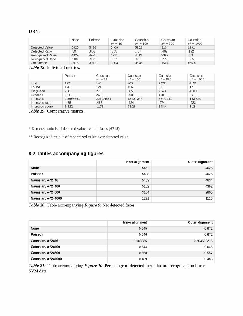
DBN:
None Poisson Gaussian
𝜎2 = 16
Gaussian
𝜎2 = 100
Gaussian
𝜎2 = 500
Gaussian
𝜎2 = 1000
Detected Value 5425 5428 5409 5152 3104 1291
Detected Ratio .807 .808 .805 .767 .462 .192
Recognized Value 4929 4925 4911 4612 2399 859
Recognized Ratio .908 .907 .907 .895 .772 .665
Confidence 3916 3912 3903 3578 1564 465.8
Table 18: Individual metrics.
Poisson Gaussian
𝜎2 = 16
Gaussian
𝜎2 = 100
Gaussian
𝜎2 = 500
Gaussian
𝜎2 = 1000
Lost 123 140 409 2372 4151
Found 126 124 136 51 17
Disguised 268 278 585 2648 4100
Exposed 264 260 268 118 30
Improved 2260/4661 2272.4651 1840/4344 624/2281 183/829
Improved ratio .485 .488 .424 .274 .223
Improved score 6.322 -1.75 73.28 198.4 112
Table 19: Comparative metrics.
* Detected ratio is of detected value over all faces (6715)
** Recognized ratio is of recognized value over detected value.
8.2 Tables accompanying figures
Inner alignment Outer alignment
None 5452 4625
Poisson 5428 4625
Gaussian, σ^2=16 5409 4634
Gaussian, σ^2=100 5152 4392
Gaussian, σ^2=500 3104 2605
Gaussian, σ^2=1000 1291 1116
Table 20: Table accompanying Figure 9: Net detected faces.
Inner alignment Outer alignment
None 0.645 0.672
Poisson 0.646 0.672
Gaussian, σ^2=16 0.668885 0.603582218
Gaussian, σ^2=100 0.644 0.646
Gaussian, σ^2=500 0.558 0.557
Gaussian, σ^2=1000 0.489 0.483
Table 21: Table accompanying Figure 10: Percentage of detected faces that are recognized on linear
SVM data.

Gaussian
𝝈𝟐 = 𝟏𝟔
Gaussian
𝝈𝟐 = 𝟏𝟎𝟎
Gaussian
𝝈𝟐 = 𝟓𝟎𝟎
Gaussian
𝝈𝟐 = 𝟏𝟎𝟎𝟎
Linear SVM -115 237 1738 2871
Radial SVM -3 328 2497 3887
Decision Tree -17 106 728 1078
Gaussian Naïve Bayes -11 301 2478 4028
DBN 18 317 2350 4070
Table 22: Table accompanying Figure 15: Net disguised values.
Gaussian
𝝈𝟐 = 𝟏𝟔
Gaussian
𝝈𝟐 = 𝟏𝟎𝟎
Gaussian
𝝈𝟐 = 𝟓𝟎𝟎
Gaussian
𝝈𝟐 = 𝟏𝟎𝟎𝟎
Decision Tree 1.010472 0.909255 0.488434 0.338295
Radial SVM 1.000651 0.928231 0.493343 0.341856
Linear SVM 1.031357 0.931015 0.531231 0.193509
Gaussian Naïve Bayes 1.002283 0.935404 0.51815 0.33789
DBN 0.996348 0.939116 0.520165 0.358066
Table 23: Table accompanying Figure 16: Normalized disguised values.
No Noise Poisson Gaussian Poisson Difference Gaussian Difference
Decision Tree 1647 1651 1664
-4 -17
Radial SVM 4609 4602 4612
7 -3
Linear SVM 3503 3508 3618
-5 -115
Gaussian Naïve Bayes 4229 4244 4261
-13 -11
DBN 4929 4925 4911
4 18
Table 24: Table accompanying Figure 18: Net disguised values (for Poisson distribution and Gaussian
𝜎2 = 16. )