Hierarchical Bayesian Models

Hierarchical Regression and Spatial models

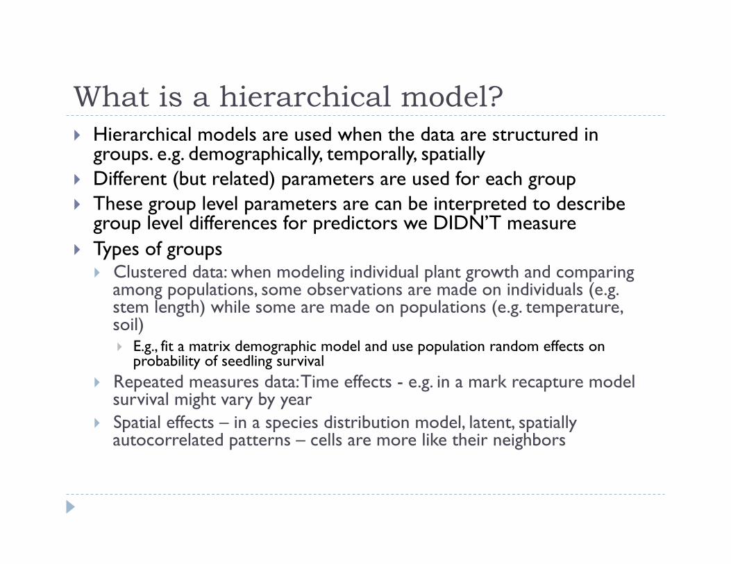
What is a hierarchical model?   Hierarchical models are used when the data are structured in

groups. e.g. demographically, temporally, spatially   Different (but related) parameters are used for each group   These group level parameters are can be interpreted to describe

group level differences for predictors we DIDN’T measure   Types of groups

  Clustered data: when modeling individual plant growth and comparing among populations, some observations are made on individuals (e.g. stem length) while some are made on populations (e.g. temperature, soil)   E.g., fit a matrix demographic model and use population random effects on

probability of seedling survival   Repeated measures data: Time effects - e.g. in a mark recapture model

survival might vary by year   Spatial effects – in a species distribution model, latent, spatially

autocorrelated patterns – cells are more like their neighbors

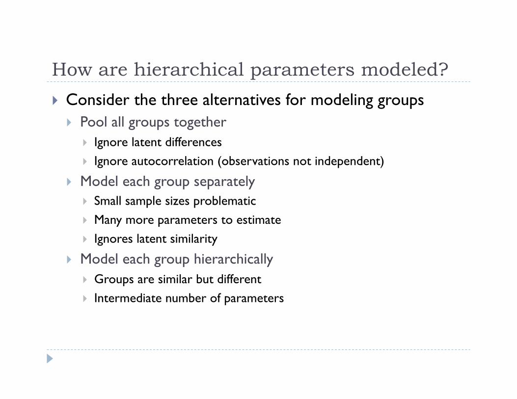
How are hierarchical parameters modeled?

  Consider the three alternatives for modeling groups   Pool all groups together

  Ignore latent differences   Ignore autocorrelation (observations not independent)

  Model each group separately   Small sample sizes problematic   Many more parameters to estimate   Ignores latent similarity

  Model each group hierarchically   Groups are similar but different   Intermediate number of parameters

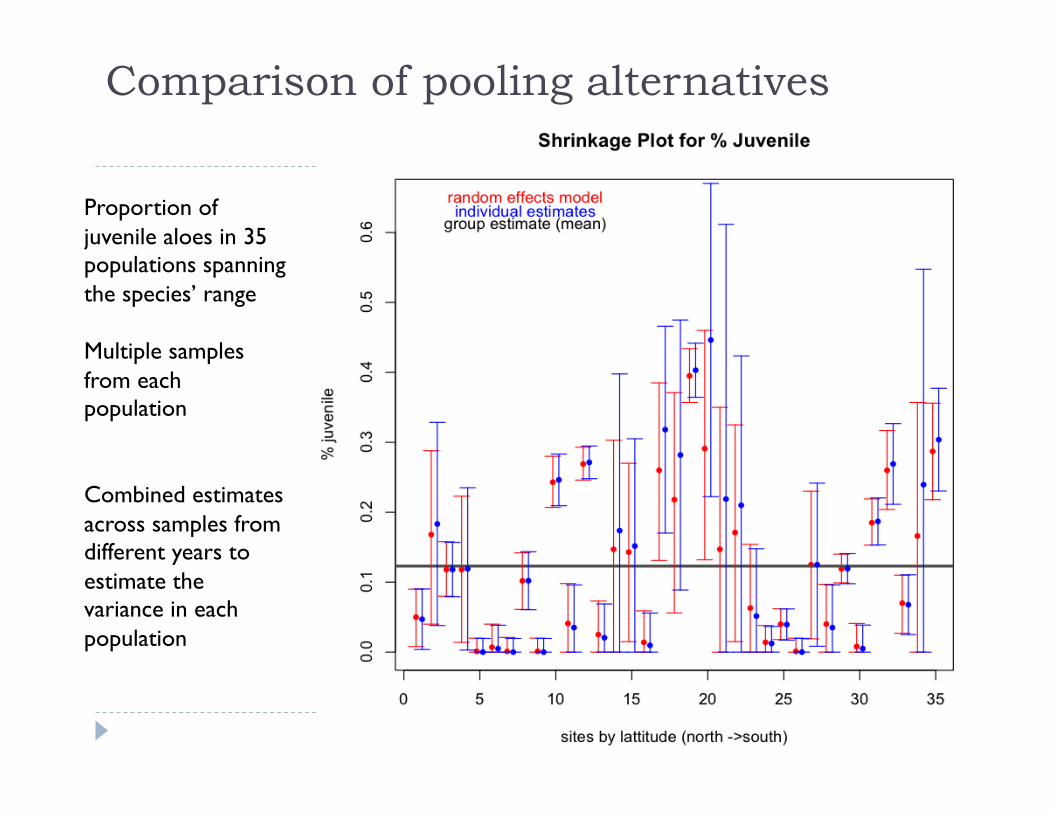
Comparison of pooling alternatives

Proportion of juvenile aloes in 35 populations spanning the species’ range

Multiple samples from each population

Combined estimates across samples from different years to estimate the variance in each population

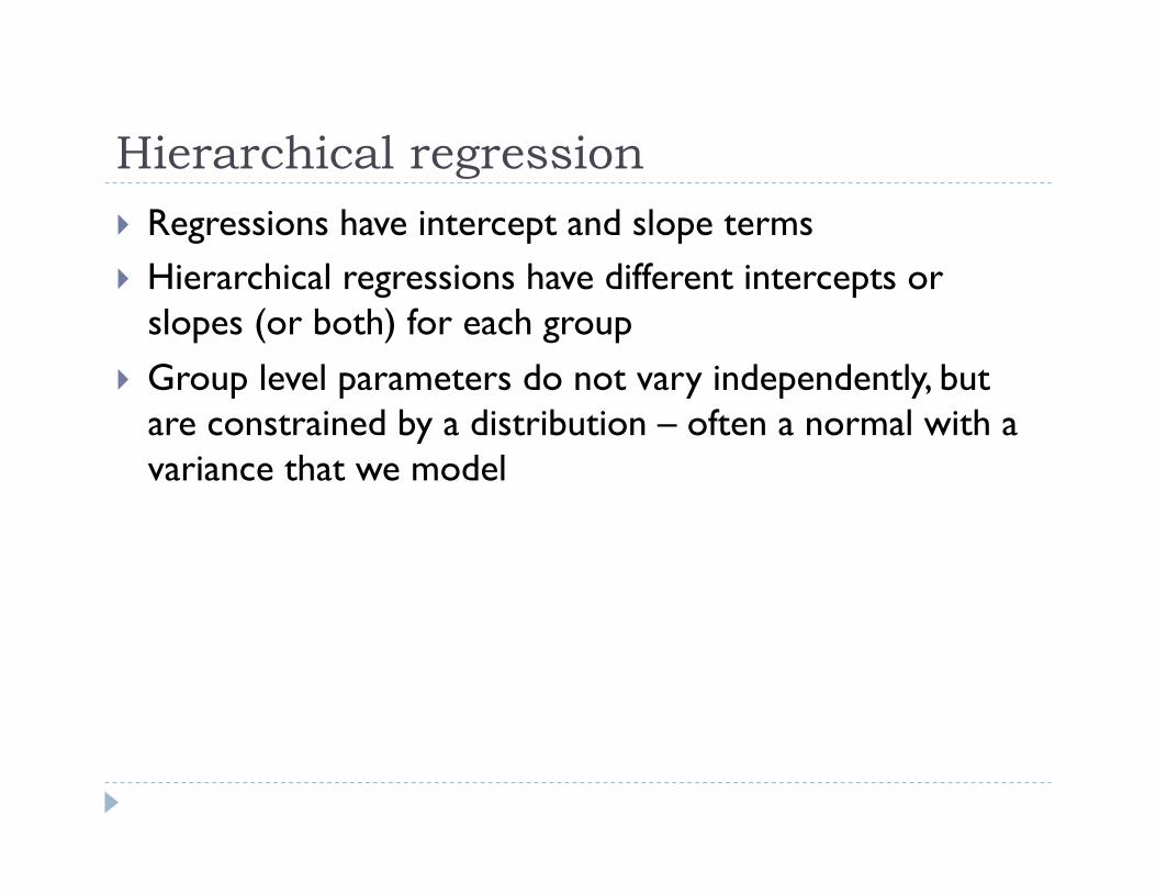
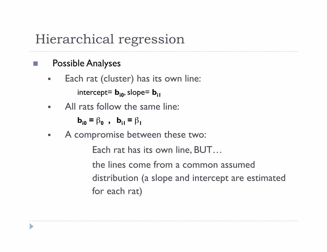
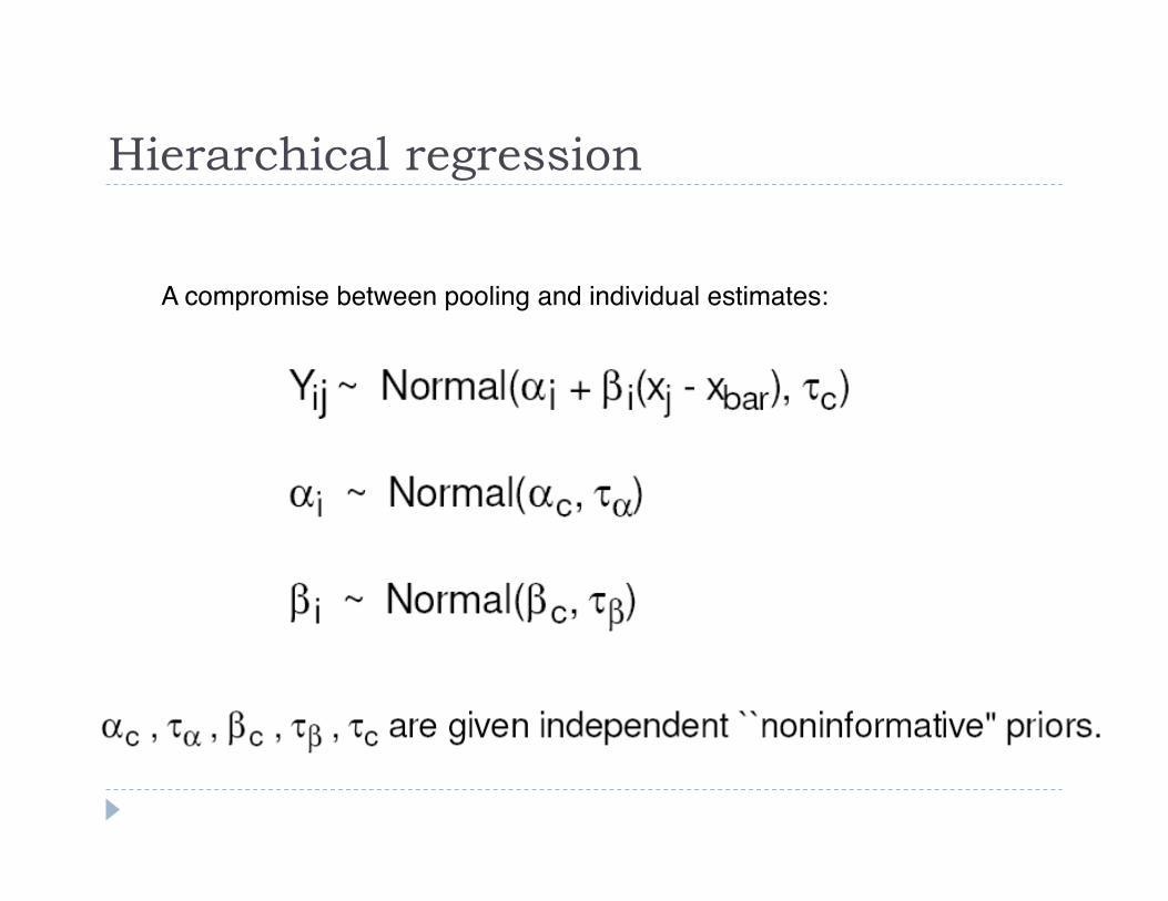
Hierarchical regression   Regressions have intercept and slope terms   Hierarchical regressions have different intercepts or

slopes (or both) for each group   Group level parameters do not vary independently, but

are constrained by a distribution – often a normal with a variance that we model

Hierarchical regression

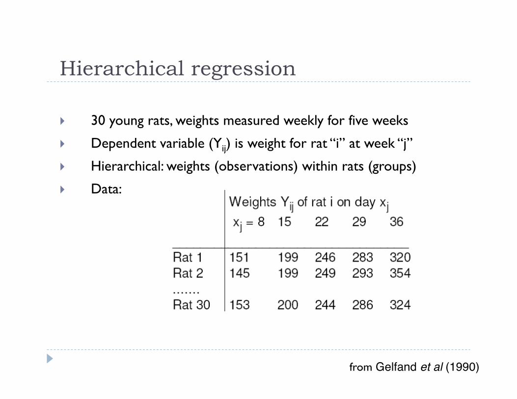
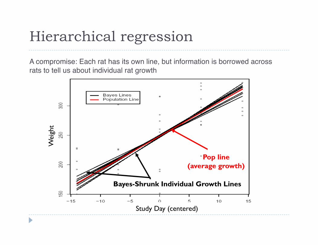
  30 young rats, weights measured weekly for five weeks

  Dependent variable (Yij) is weight for rat “i” at week “j”

  Hierarchical: weights (observations) within rats (groups)

  Data:

from Gelfand et al (1990)"

Hierarchical regression

Hierarchical regression

Pop line (average growth)

Individual Growth Lines

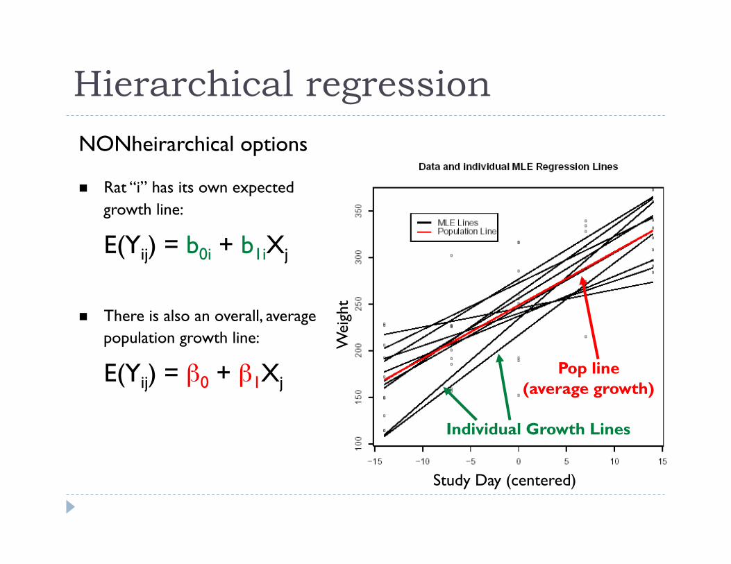
  Rat “i” has its own expected growth line:

E(Yij) = b0i + b1iXj

  There is also an overall, average population growth line:

E(Yij) = β0 + β1Xj

Wei

ght

Study Day (centered)

NONheirarchical options

Hierarchical regression

A compromise between pooling and individual estimates:"

Pop line (average growth)

Bayes-Shrunk Individual Growth Lines

Hierarchical regression W

eigh

t

Study Day (centered)

A compromise: Each rat has its own line, but information is borrowed across rats to tell us about individual rat growth"

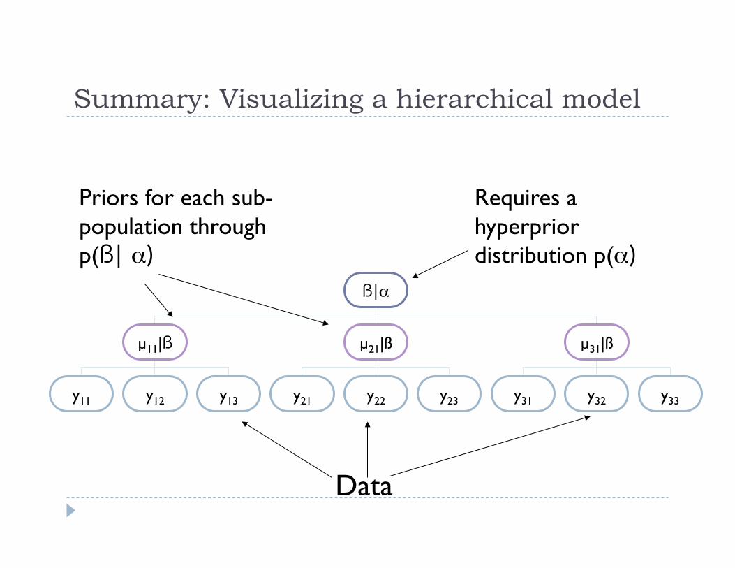
Summary: Visualizing a hierarchical model

ß|α

µ11|ß µ21|ß µ31|ß

y11 y12 y13 y21 y22 y23 y31 y32 y33

Requires a hyperprior distribution p(α)

Priors for each sub-population through p(ß| α)

Data

Summary: Visualizing a hierarchical model

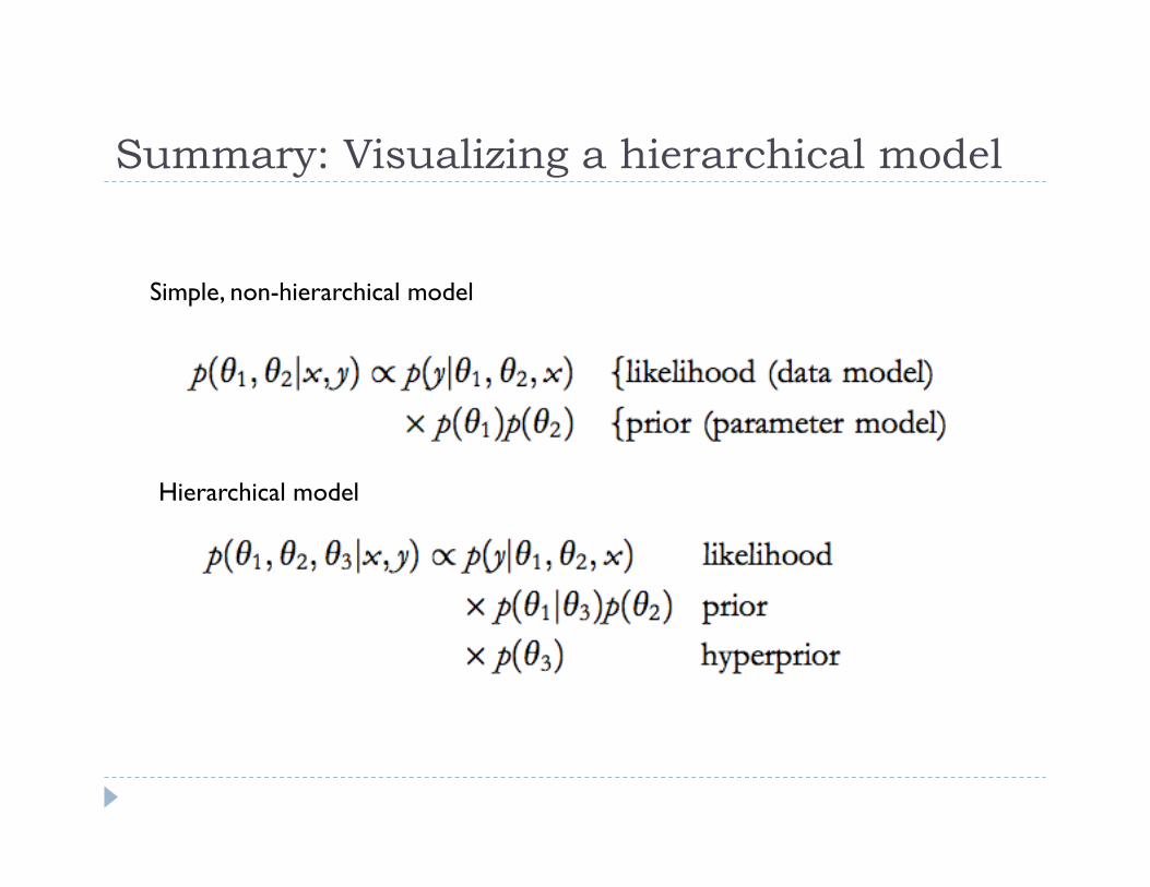
Simple, non-hierarchical model

Hierarchical model

Why use hierarchical models?   Account for sources of uncertainty/variability

  Account for individual level and group level variation when estimating group level coefficients (classical models require averaging over individual level variation)

  Borrow strength across groups (minimize effects of small sample sizes in some groups)

  Random effects absorb variation that’s NOT related to the fixed effects so you potentially get lower bias for fixed effect estimates

  Random effects pick up unmeasured variation   It’s probably never worse than nonhierarchical models because

the worst case is that you find among group variation to be irrelevant

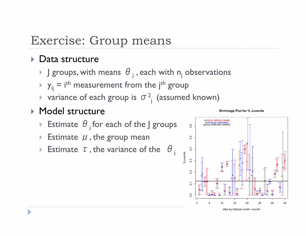
Exercise: Group means   Data structure

  J groups, with means θj , each with nj observations   yij = ith measurement from the jth group   variance of each group is σ2

j (assumed known)

  Model structure   Estimate θj for each of the J groups   Estimate μ, the group mean   Estimate τ, the variance of the θj

Formalizing the group means model   Data structure

  J groups, with means θj , each with nj observations   yij = ith measurement from the jth group   variance of each group is σ2

j (assumed known)   εij = error εij ~ N(0,σ2)

  Model structure   Estimate θj for each of the J groups   Estimate μ, the group mean   Estimate τ, the variance of the θj

  All groups the same   yij = µ + εij

  Each group unique   yij = θj + εij

  Compromise: Groups similar but different   yij = θj + εij, with: θj ~ N(µ,τ2)

See Ch. 5 of Gelman et al. 2005. Bayesian Data Analyis for details of this model

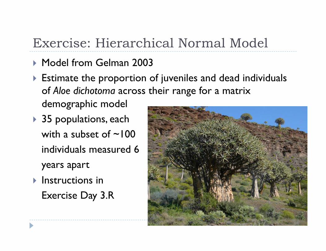
Exercise: Hierarchical Normal Model   Model from Gelman 2003   Estimate the proportion of juveniles and dead individuals

of Aloe dichotoma across their range for a matrix demographic model

  35 populations, each with a subset of ~100 individuals measured 6 years apart

  Instructions in Exercise Day 3.R

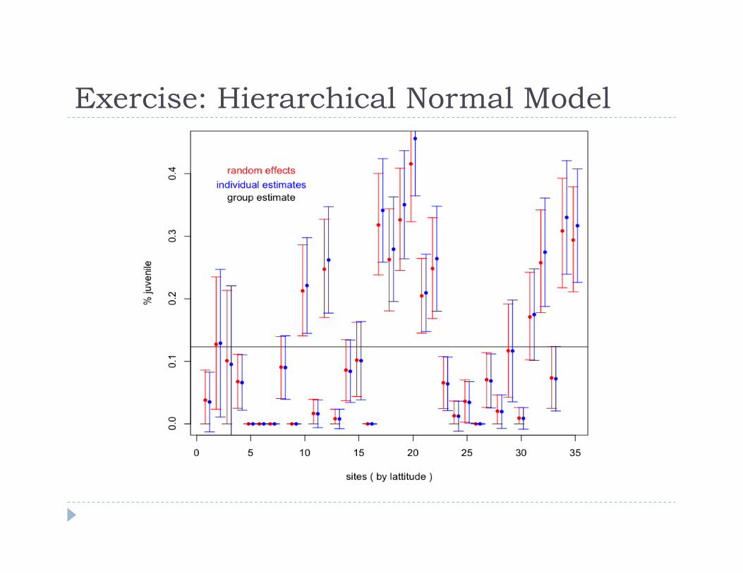
Exercise: Hierarchical Normal Model

Outline   Review   Continuation of exercises from last time   Hierarchical model   Spatial models

18

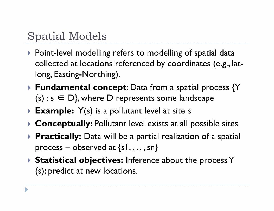
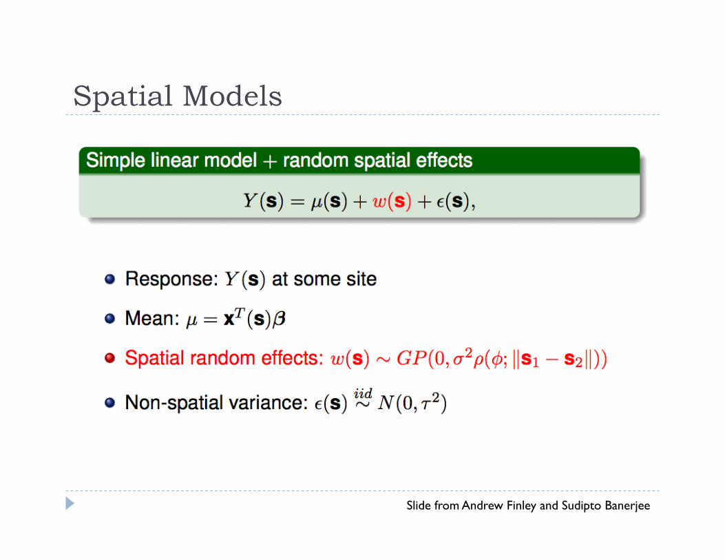
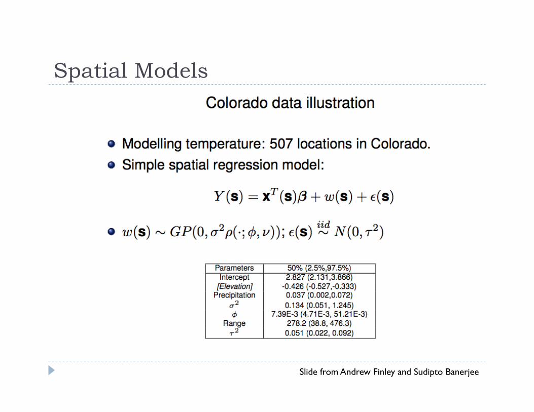
Spatial Models   Point-level modelling refers to modelling of spatial data

collected at locations referenced by coordinates (e.g., lat-long, Easting-Northing).

  Fundamental concept: Data from a spatial process {Y (s) : s ∈ D}, where D represents some landscape

  Example: Y(s) is a pollutant level at site s   Conceptually: Pollutant level exists at all possible sites   Practically: Data will be a partial realization of a spatial

process – observed at {s1, . . . , sn}   Statistical objectives: Inference about the process Y

(s); predict at new locations.

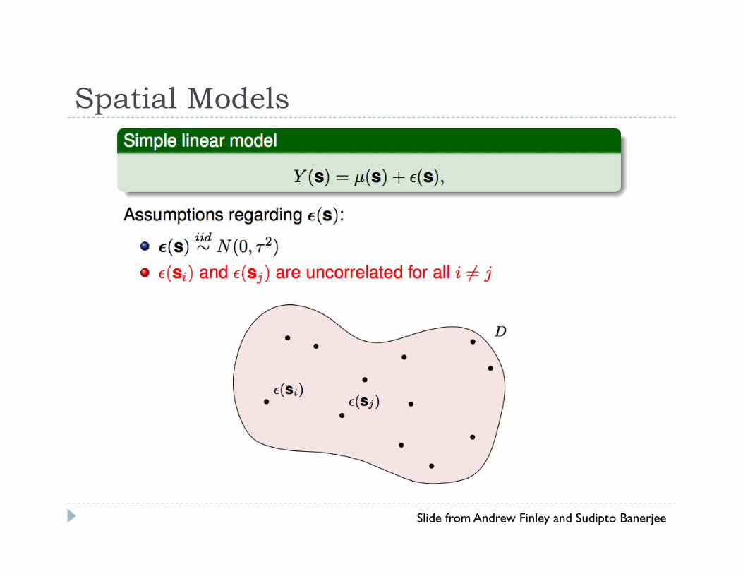
Spatial Models

Slide from Andrew Finley and Sudipto Banerjee

Spatial Models

Slide from Andrew Finley and Sudipto Banerjee

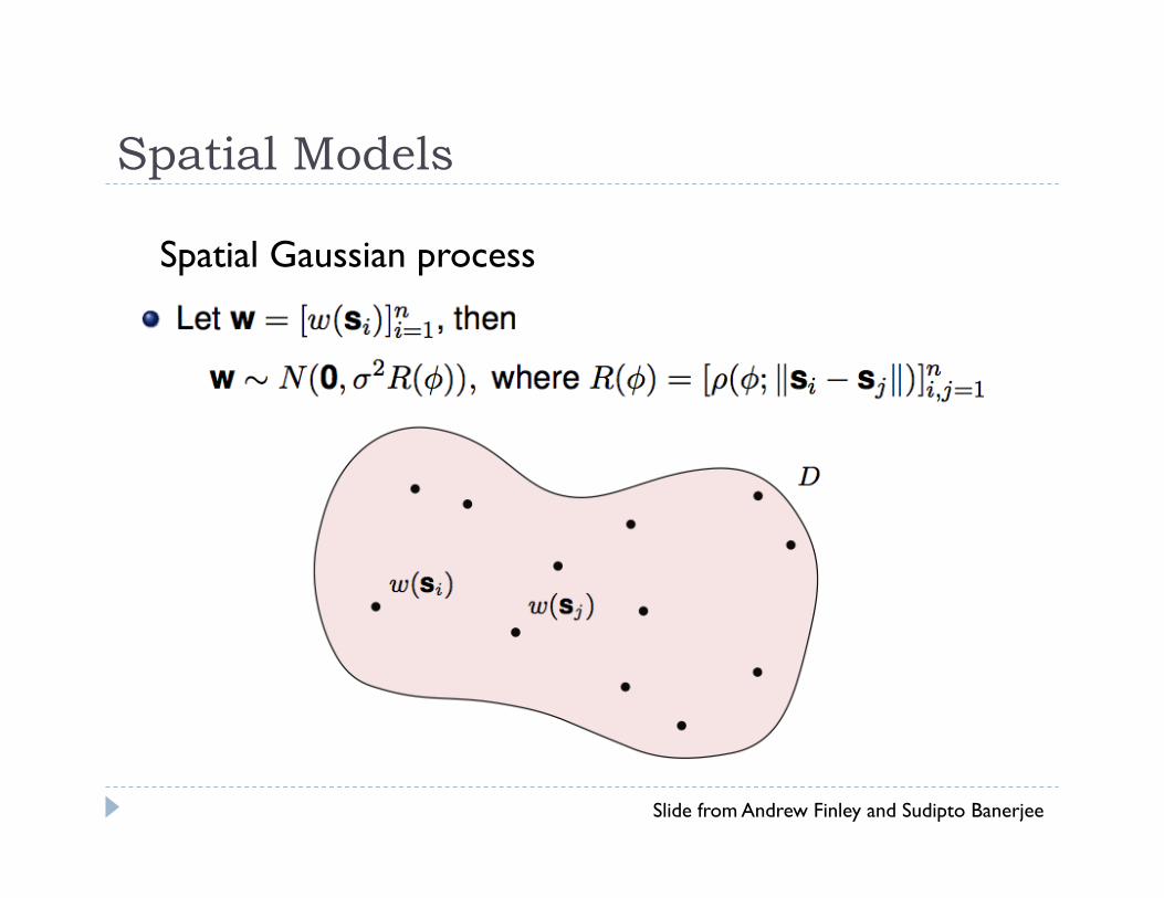
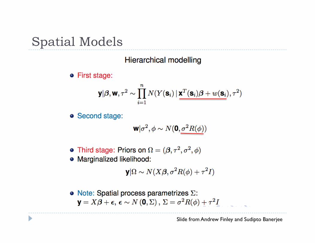
Spatial Gaussian process

Spatial Models

Slide from Andrew Finley and Sudipto Banerjee

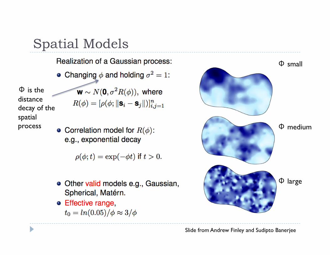
Φ is the distance decay of the spatial process

Φ small

Φ medium

Φ large

Spatial Models

Slide from Andrew Finley and Sudipto Banerjee

Spatial Models

Slide from Andrew Finley and Sudipto Banerjee

Spatial Models

Slide from Andrew Finley and Sudipto Banerjee

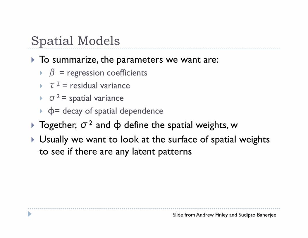
  To summarize, the parameters we want are:   β = regression coefficients   τ2 = residual variance   σ2 = spatial variance   ϕ= decay of spatial dependence

  Together, σ2 and ϕ define the spatial weights, w   Usually we want to look at the surface of spatial weights

to see if there are any latent patterns

Spatial Models

Slide from Andrew Finley and Sudipto Banerjee

Spatial Models

Slide from Andrew Finley and Sudipto Banerjee

Spatial weights w/elevation

Spatial weights w/o elevation

Spatial Models

Slide from Andrew Finley and Sudipto Banerjee

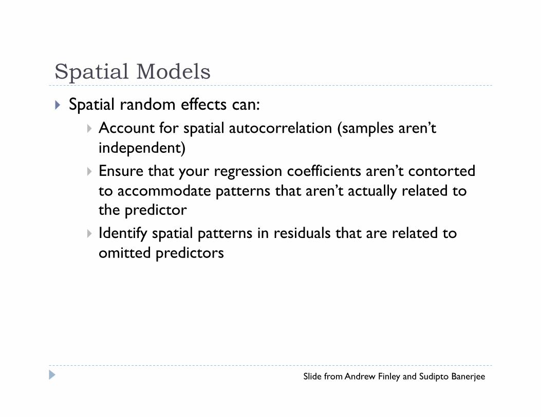
  Spatial random effects can:   Account for spatial autocorrelation (samples aren’t

independent)   Ensure that your regression coefficients aren’t contorted

to accommodate patterns that aren’t actually related to the predictor

  Identify spatial patterns in residuals that are related to omitted predictors

Exercise: Spatial Models

Slide from Andrew Finley and Sudipto Banerjee

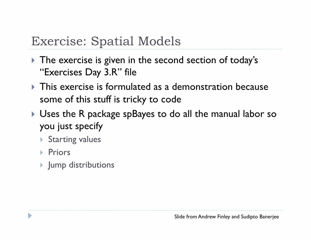
  The exercise is given in the second section of today’s “Exercises Day 3.R” file

  This exercise is formulated as a demonstration because some of this stuff is tricky to code

  Uses the R package spBayes to do all the manual labor so you just specify   Starting values   Priors   Jump distributions

30

Conclusions

  Model 1   Prior: Bayesian methods are extremely complicated   Data: Go to a Bayesian workshop   Posterior: Bayesian methods aren’t too bad†

  Model 2   Prior: Posterior from step 1   Data: Read Bayesian Books   Posterior: Use Bayesian Methods†

† Metropolis-Hastings sampling recommended