hierarchical forecasting of web server workload using sequential monte ... · hierarchical...

1286 IEEE TRANSACTIONS ON SIGNAL PROCESSING, VOL. 55, NO. 4, APRIL 2007

Hierarchical Forecasting of Web Server WorkloadUsing Sequential Monte Carlo Training

Tom Vercauteren, Pradeep Aggarwal, Xiaodong Wang, Senior Member, IEEE, and Ta-Hsin Li, Senior Member, IEEE

Abstract—Internet service utilities host multiple server applica-tions on a shared server cluster (server farm). One of the essentialtasks of the hosting service provider is to allocate servers to each ofthe websites to maintain a certain level of quality of service for dif-ferent classes of incoming requests at each point of time, and opti-mize the use of server resources, while maximizing its profits. Sucha proactive management of resources requires accurate predictionof workload, which is generally measured as the amount of servicerequests per unit time. As a time series, the workload exhibits notonly short time random fluctuations but also prominent periodic(daily) patterns that evolve randomly from one period to another.We propose a solution to the Web server load prediction problembased on a hierarchical framework with multiple time scales. Thisframework leads to adaptive procedures that provide both long-term (in days) and short-term (in minutes) predictions with si-multaneous confidence bands which accommodate not only serialcorrelation but also heavy-tailedness, and nonstationarity of thedata. The long-term load is modeled as a dynamic harmonic regres-sion (DHR), the coefficients of which evolve according to a randomwalk, and are tracked using sequential Monte Carlo (SMC) algo-rithms; whereas the short-term load is predicted using an autore-gressive model, whose parameters are also estimated using SMCtechniques. We evaluate our method using real-world Web work-load data.

Index Terms—Dynamic harmonic regression, seasonal time se-ries, sequential Monte Carlo, Web-load prediction.

I. INTRODUCTION

AWEB server farm is a cluster of servers shared by severalWeb applications and services and maintained by a host

service provider. Usually, the owner of the Web applicationspays the host service provider for the computing resourcesand, in return, gets a quality-of-service (QoS) guarantee, whichpromises a certain minimum level of resources and perfor-mance. Static allocation of resources at the server farm is notefficient since very often it results in either underutilization ofresources (when the particular Web application is not activelybeing sought) or violation of QoS (when, for example, trafficfor a particular website is very high and the allocated sourcesare insufficient to cater to the demands). Therefore, the serverfarm allocates the computing resources dynamically amongthe competing applications to meet the quality-of-service fordifferent classes of service requests, while at the same time

Manuscript received November 12, 2005; revised June 23, 2006. The asso-ciate editor coordinating the review of this paper and approving it for publicationwas Prof. Steven M. Kay.

T. Vercauteren is with INRIA, 06902 Sophia Antipolis, France.P. Aggarwal and X. Wang are with Department of Electrical Engineering,

Columbia University, New York, NY 10027-4712 USA (e-mail: [email protected]).

T.-H. Li is with Department of Mathematical Sciences, IBM T. J. WatsonResearch Center, Yorktown Heights, NY 10598 USA.

Digital Object Identifier 10.1109/TSP.2006.889401

striving to maximize its own profits. The requirement fordynamic allocation of resources makes it necessary for theserver farm to be able to predict the workload accurately, with asufficiently long time horizon to ensure that adequate resourcesare allocated to the services in-need in a timely manner, whilestill achieving certain systemwide performance objective suchas maintaining the QoS requirements of the entire server farmand maximizing the total revenue of the server farm under theQoS constraints. In a typical dynamic allocation scheme, eachapplication is provided a certain minimum share of resources,and the remaining resources (servers and bandwidth) are dy-namically allocated to the different active applications basedon their instantaneous requirements and based on predefinedpolicy in response to the workload changes. The predictiontechniques/models are also helpful in preventing imminentservice disruptions by anticipating potential problems due toheavy load on a particular website [1]–[5].

The server workload is usually measured in terms of theamount of services request per unit time (also called the re-quest arrival rate). It can, for example, be the total number orsize of the files requested per unit time, or it can be the totalnumber of operations requested per unit time. A time series ofsuch a workload is known to vary dynamically over multipletime scales, and therefore it is quite challenging to predictit accurately. In particular, the bursty nature and the nonsta-tionarity of the server workload impose inherent limits on theaccuracy of the prediction. Such a time series can, for example,be stationary but self-similar (i.e., the correlational structureremains unchanged over a wide range of time scales, resultingin long-range dependence, or in other words, it exhibits burstswherein the workload remains above the mean for an extendedduration at a wide range of time scales) and/or heavy-tailed oversmall duration (seconds or minutes) at a fine time granularity[6]–[9]; it can also exhibit strong daily and weekly patterns(seasonality), which change randomly over different times ofthe day and different days of the week, and can also showcalendar effects (different patterns on weekends) [8]–[10]. It isthis second type of data with seasonal variations that is key tothe designing of dynamic resource allocation schemes and isthe focus of the current paper.

The traditional linear-regression-based methods can givepredictions with a limited accuracy, since the model can be-come inefficient in the presence of correlated error. In thispaper, we follow the hierarchical approach proposed in [11]and [12] in which the time-series prediction is decomposed intotwo steps: first a prediction of the long-term component, whichprimarily captures the nonstationarity of the data, is performed,and then the residual short-term process, which captures boththe long-term prediction error and the short-term component ofthe time series, is processed. As demonstrated by the results,the two-scale decomposition captures the underlying statistics

1053-587X/$25.00 © 2007 IEEE

VERCAUTEREN et al.: HIERARCHICAL FORECASTING OF WEB SERVER WORKLOAD USING SEQUENTIAL MONTE CARLO TRAINING 1287

of the data fairly well. Additional components (e.g., weekly ormonthly seasonality) increase the complexity of the algorithmas we have to estimate more parameters now. Furthermore, theyalso require much more training data. One of the main aims ofthis paper is to keep the computational complexity low, whichour sequential Monte Carlo (SMC) algorithm-based two-scalescheme indeed achieves, without compromising the accuracy ofthe prediction. For example, the dynamic harmonic regression(DHR) model in [13] estimates the parameters by first runninga two-step (prediction–correction) Kalman filter, followedby a fixed-interval smoothing algorithm. As the number ofparameters increases, these steps become highly complex asthey involve multiplication and inversion of high-dimensionalmatrices, whereas in the proposed SMC algorithm, the com-plexity increases only linearly with the number of parameters tobe estimated. Previous literature, e.g., [11]–[13], also stronglymentions that not all the components of the unobserved com-ponent (UC) model are required for modeling the Web-serverworkload data and that the two-scale modeling is a good com-promise between accuracy and computational complexity ofthe algorithm.

In this paper, the long-term component is modeled as a linearcombination of certain basis functions with random amplitudesevolving with time, while the residual short-term process ismodeled as a traditional autoregressive (AR) process. Theshort-term prediction is useful in predicting abnormalities inthe workload data and to take care of rapid fluctuations, therebygiving the server farm management system sufficient time toprevent the possible disruption of services [11]. In this paper,in addition to the traditional short-term prediction, we alsoderive a scheme to predict the long-term component, utilizingthe daily patterns in the workload time series. This not onlyprovides ample time for advance planning, but also reduces themagnitude (and hence complexity) of the short-term adjustmentthat needs to be made in case of an imminent (potential) disrup-tion. Moreover, the proposed method, in addition to providingpredictions, can also be used to compute confidence bandssimultaneously. This is of major interest in this setting sincequantiles, as opposed to a simple prediction of the time series,can be used to support flexible (probability based) service-levelagreements. Further, the proposed model allows the modelparameters to change with time, thereby making itself capableof handling the nonstationarity in the data.

For the long-term component, we combine the DHR frame-work of [13] together with the filter bank approach of [14],to decompose the time series into seasonal components andonly those basis functions that show high coherence across theperiods are selected for long-term modeling and forecasting pur-pose. The use of highly coherent basis functions not only re-duces the dimensionality of the problem, but also results inreliable long-term forecasting by using only the persistent com-ponents. This, in turn, results in reduction of the amount oftraining data required as well as making the model robust to theimpact of noise and occasional corruption of training data. Asmentioned before, the long-term component is represented asa linear combination of the basis functions, whose amplitudesare modeled as random processes under the state-space setting,the dynamic nature of which allows them to efficiently capturethe trends and fluctuations of the data. Moreover, to take careof the calendar effect (e.g., the weekend data follows differenttrends as compared to the weekday data), a multiregime model

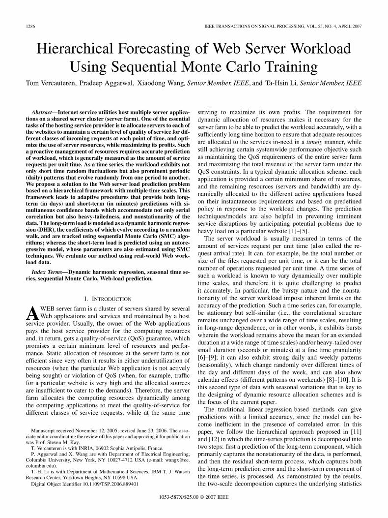
Fig. 1. Total file size (in log of bytes of HTTP requests), aggregated over� = 5-min intervals, received at a Web server of an online retail store over13 days.

is employed, in which the data belonging to different regimes ishandled separately (using similar scheme nonetheless). The pa-rameters for both the short-term model and the long-term modelare estimated using the SMC methods, which are very powerfulstatistical tools for dealing with online estimation problems indynamic systems (see [15]–[17] and references therein) and findapplications in diverse fields.

The remainder of the paper is organized as follows. Section IIdiscusses the properties of the time series at hand and explainsthe hierarchical structure of our model. In Section III, we de-scribe the dynamic harmonic regression based model for thelong-term components and the long-term prediction using theSMC methods. Section IV deals with the modeling and predic-tion of the short-term component. Simulation results are pre-sented in Section V; and Section VI concludes the paper.

II. HIERARCHICAL FRAMEWORK

We consider a typical Web-server farm, which records thenumber of requests at each server and aggregates them oversmall time intervals of length to obtain a time series.For example, Fig. 1 shows the server workload obtained byaggregating the hypertext transfer protocol (HTTP) service re-quests for a commercial website over 5-min intervals overa 13-day period, giving a total of 288 intervals in a day. This isthe same data as used in [12], and we will employ this time seriesthroughout this paper as a working example to demonstrate theperformance of the proposed algorithm. The time series is firstconverted into logarithmic domain to reduce the dependence ofthe local variability on the local mean of the untransformed data.

Clearly, the data is nonstationary in that the mean changeswith time of day and day of week. It is also observed thatthe time series shows predominant daily patterns, varyingrandomly. Let denote the sampling frequency (number ofsamples per period) of the daily pattern. For the example shownin Fig. 1, for 5 min, . Note that for a given , thetime index for the observation in the th time interval in the thperiod is given by , and .Although, several methods exist for modeling such a time se-ries, we follow the hierarchical approach developed in [12],


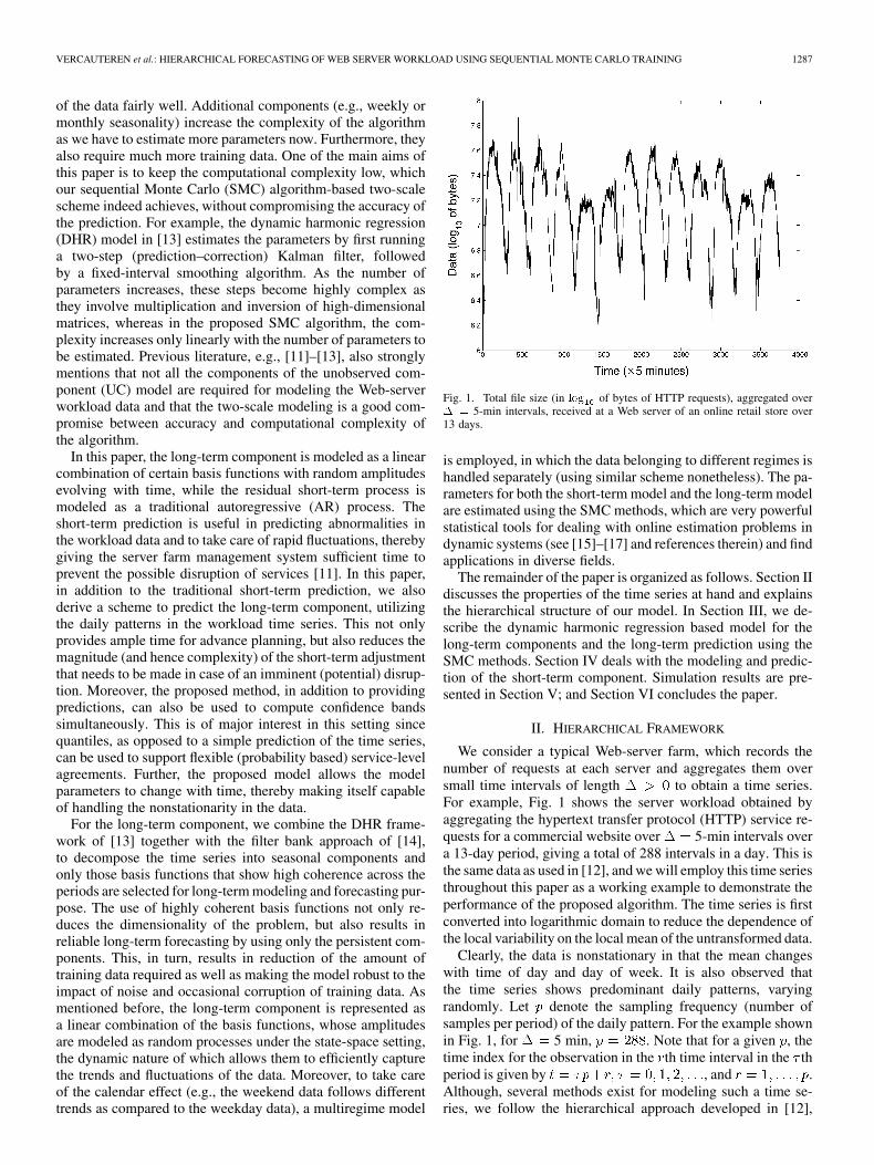
Fig. 2. Decomposition of the Web-server data into a long-term pattern andshort-term random components.

which not only provides point predictions, but also simulta-neous confidence bands, that can be used to support flexible(probability-based) service-level agreements. Furthermore, byallowing the model parameters to change with time, we canhandle nonstationarity in both the long-term patterns as wellas short-term fluctuations. Moreover, the hierarchical approachallows for easy diagnostic checking of model adequacy. Fig. 2shows the hierarchical structure of the time series, where thedata is decomposed into a periodic long-term component and arandomly fluctuating short-term component.

Let denote the observed load (after taking logarithm)at a server at time . In order to capture the seasonality in thedata, we use the DHR model of [13]. The DHR model is a spe-cial type of the unobserved component model and can be usedto capture several components such as trend, cyclical compo-nent, and seasonality. Stochastic time-varying parameters areused to characterize the various components of the DHR, thusallowing for nonstationarity in the resulting time series. In prac-tice, not all components of the DHR are necessary, and in thispaper, we focus on the seasonal component. In our hierarchicalframework, the time series is first modeled as a combination of aperiodic long-term pattern , and a more irregular short-termcomponent

(1)

The periodic long-term pattern is represented as aweighted sum of some -periodic basis functions as

(2)

where are stochastic time-varying parameters andforms a subset of some set of linearly independent

basis functions . In contrast with [13], our modelalso deals with a time-varying set of basis functions . Atthis point of the model, we are only interested in obtaining anestimation of the long-term component; the short-term compo-nent will therefore be roughly modeled as a white noiseterm. To filter out the long-term component in (1), we choosethe periodic basis functions to be sinusoidal waves whose

frequencies are chosen based on the spectral properties of thetime series [this is discussed further in Section 3-A-1)], givingus a harmonic regression (HR) on the long-term component.Moreover, an extra zero-frequency term is also added that canbe considered as a stochastic time-variable “intercept” in theDHR.

Once the long-term estimation has been performed, ourhierarchical framework focuses on making an accurate -stepahead forecast of the residual time series

(3)

This -step-ahead forecast process is modeled as an AR process

(4)

the parameters of which (order, coefficients, and noise charac-teristics) being stochastic time-varying parameters as in [18].Furthermore, in order to accommodate for the shot noises in thedata, we use heavy-tailed distributions for the noise term .

The observation models (1), and (4), together with their dy-namically varying coefficients form two dynamic state spaces,both are tracked using SMC methods.

For the time series of service requests, it is typical to haveweekday patterns behaving significantly differently from theweekend patterns. In this paper, a multiple-regime approachis employed, in which data belonging to different regimes aremodeled separately to take advantage of the within-regime re-semblance, taking care of the between-regime change at thesame time. The data belonging to the same regime is cascadedto obtain a set of new time series, one for each regime. For ourexample of Fig. 1, all weekday data can be collected togetherto form a weekday time series and all weekend data can be col-lected to form a new weekend series. Each time series is thenmodeled by (1) and (4). Each regime has its own set of pa-rameters and some of them may be shared across the regimesto ensure smooth transition when the regime shifts. Note thatsometimes, under the assumption that the short-term compo-nent do not change substantially with regime shifts, it is moreconvenient and justifiable to merge the short-term componentsin all regimes to obtain a single time series for modeling andprediction.

The remainder of the paper discusses in detail the modeling,parameter estimation, and prediction based on the model de-scribed above.

III. LONG-TERM MODELING AND PREDICTION

Since we deal with different regimes separately, it is sufficientto consider only a single regime and assume that the statisticalproperties do not change abruptly with regime shift. We alsoassume that the type of basis functions in (2) are knowna priori (e.g., sinusoids, wavelets, etc.) and that the largest al-lowed set of basis functions does not change with time.

Selection of the basis set serves a dual purpose. First, itreduces the dimensionality of the problem, hence reducing thecomputational complexity as well as storage requirement asso-ciated with the training, modeling, and prediction. Indeed, thehigher the dimension is, the greater the number of parametersto be estimated is. The need for reduction in dimension be-comes more important in Web-server management as compared


to, say, economic forecasting [19] or electric utility management[20]–[22], due to the sheer number of parameters that are to beestimated, resulting from the much finer time granularity (min-utes rather than hours or days). For example, for 5 min,we get a sampling frequency of 288 steps and for 1min, , as compared with for hourly data withdaily seasonality, and for monthly data with yearly sea-sonality. The second advantage of selecting lies in the factthat it makes the modeling and prediction more robust to esti-mation errors as compared with the model with a large basisset . Statistical theory of regression analysis [23] asserts thatin the presence of inherent statistical error in parameter estima-tion, the mean-square error associated with both modeling andprediction can be reduced by simply dropping the “minor” com-ponents even if they exist in reality.

We will see in Section 3-A-1) that only the first few frequen-cies (including the zero-frequency term) affect the seasonal vari-ations to any significant extent and that only a fixed number ofsinusoids need to be in . It turns out that usually even withinthis fixed subset, only a few among those chosen frequency com-ponents are significant in representing the model at a particulartime , while the remaining ones carry relatively small weightsand, hence, can be discarded without significant loss in perfor-mance. However, the important subset of can change withtime. Therefore, instead of accommodating all of them in ourmodel, we can reduce the dimensionality further by dynamicallyselecting the frequencies from the set , as the system evolves.We follow the jump Markov framework of [18], which is closeto the resampling-based shrinkage method proposed in [24] inthe context of blind detection in fading channels.

Let us now write down the state-space form we use for thelong-term model

(5)

where is the process noise, is themeasurement noise, and is the observed data. The secondequation in (5) represents the first-order Markov transitionprocess, which is assumed to generate the coefficients vector

. The vector represents temporallyuncorrelated Gaussian disturbances with zero mean, and co-variance matrix , i.e.,

and (6)

The zero-mean noise in the state equation stems from theassumption that the long-term behavior is periodic with slowvariations, for which, the incremental mean of the coefficientsis close to zero. The first equation in (5) represents the mea-surement equation, where is the temporally uncorrelatedGaussian disturbance with zero mean and variance , i.e.,

and (7)

The initial state vector is assumed to be Gaussian dis-tributed with mean and covariance matrix , i.e.,

and (8)

which are computed as the respective mean and covariance ofthe coefficients of the harmonics included in the regression, ob-tained from the training data. Further, the disturbance and

are assumed to be uncorrelated with each other in all timeperiods and uncorrelated with the initial state, i.e.,

for all

and

for all (9)

In (5), we chose to use a dynamic subset of harmonics .This subset is assumed to follow a first-order discrete Markovmodel

(10)

where the are some subsets of .In what follows, we explain how the fixed parameters of our

model and the set of basis functions are determined fromthe historical observations of , and in Section III-B, wedemonstrate how SMC methods can be employed to track thisstate-space model and select the subset dynamically.

A. Determination of the Fixed Parameters

We use the analysis filter bank approach proposed in [14] topredetermine the basis set and guide our choice of fixed pa-rameters (priors, variances). The aim is to decompose the timeseries into seasonal components and consider only those com-ponents that are highly coherent across the period, as well ashaving high energy, and hence are important to modeling andprediction. In order to do this, we consider, at each time step,a single time period ending at the given time step and pass itthrough a filter bank. The resulting series of coefficients can thenbe analyzed.

Let be the dataat hand. Then, from (2), using the full basis, we can write

(11)

where are the coefficients associ-ated with the complete basis decomposition,is the matrix of all the basis functions, and its inverse has ananalysis filter bank interpretation. In other words, denoting theth row of by , (11) can be

written as

(12)

which is nothing but the output obtained on passing througha filter bank consisting of finite-impulse-response (FIR) filters,with being the impulse response of theth filter. After having obtained the analysis filter bank output

defined in (12), the data can be reconstructed ac-cording to

(13)

which can be considered as the decomposition of into com-ponent waveforms, whose shapes are determined by the basisfunctions .


1) Choice of Basis Set: Clearly, with being very large( for our example), we aim to reduce the dimensionsof the filter bank and chose by analyzing . In [12], twomeasures on the component waveforms are suggested to quan-tify the behavior of to aid in the selection of , namely,the coherence measure and the energy measure. The coherencemeasure is defined as

(14)

where is the sample mean and is the sample variance of, obtained as

and

(15)

The th waveform is said to be completely coherent if ,and incoherent if . We seek to include highly coherentwaveforms (waveforms with high values of ) in as they havelong-lasting effects, making them good candidates for long-termforecasting. The energy measure of the component waveformsis defined as

(16)

High-energy components along with high-coherence compo-nent are crucial to effective modeling of and are includedin . For future reference, let the number of basis functions in-cluded in be .

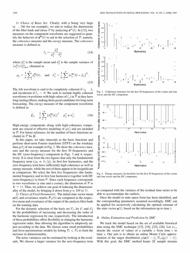
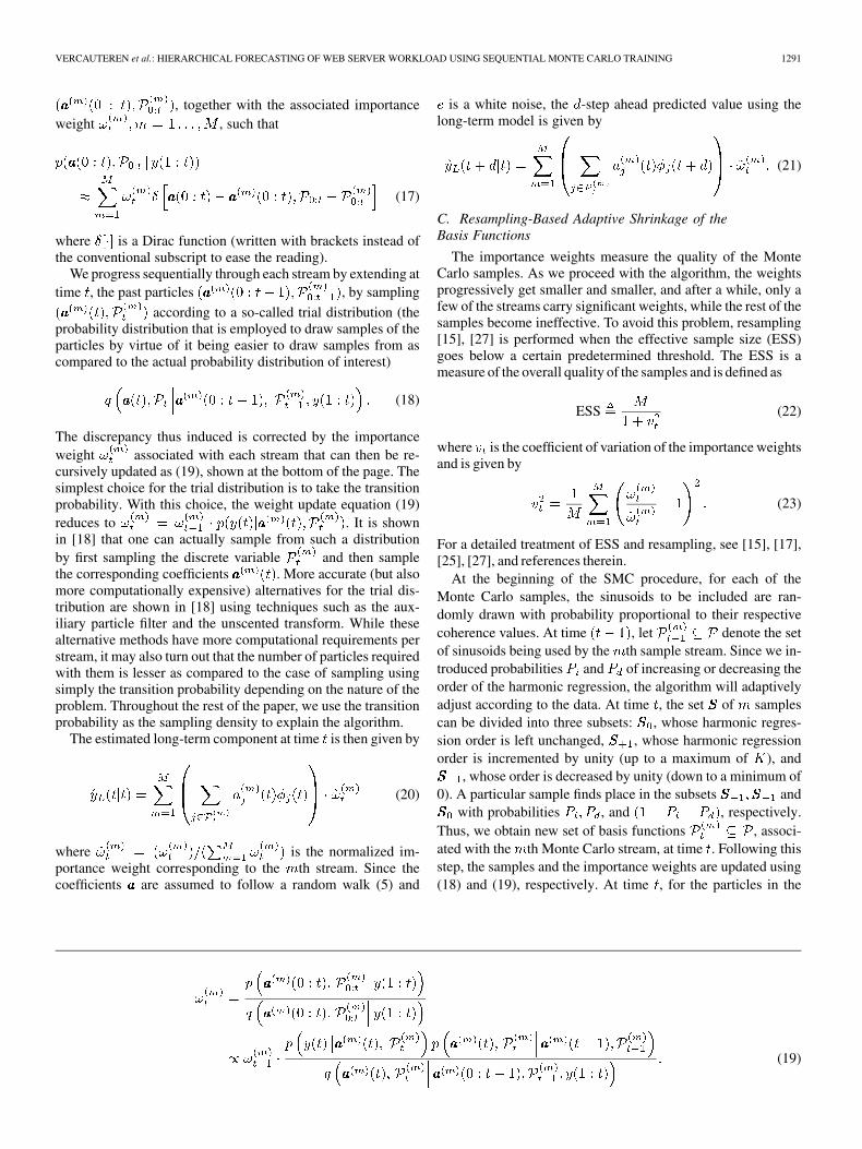
In this paper, we take sinusoids as the basis functions andperform short-term Fourier transform (STFT) on the weekdaydata of our example in Fig. 1. We show the coherence mea-sure and the energy measure for the first 30 frequencies andthe DC (zero-frequency) component in Figs. 3 and 4, respec-tively. It is clear from the two figures that only the fundamentalfrequency term , its first few harmonics, and thezero-frequency term have sufficiently high coherence as well asenergy measure, while the rest of them appear to be insignificantin comparison. We select the first five frequencies (the funda-mental frequency and its first four harmonics) together with DC(zero-frequency) to form . Since each frequency correspondsto two waveforms (a sine and a cosine), the dimension of is

. Thus, we achieve our goal of reducing the dimension-ality of the model, by bringing it down from to .

2) Choice of Fixed Parameters: The initial state vector meanand covariance matrix are computed as the respec-

tive mean and covariance of the output of the analysis filter bankon the training data.

For the dynamic selection of the basis set , let andbe the probabilities of increasing and decreasing the order ofthe harmonic regression by one, respectively. The introductionof these probabilities offers flexibility in changing the harmonicregression order, thus allowing the algorithm to adaptively ad-just according to the data. We choose some small probabilitiesand favor parsimonious models by letting to limit theincrease in dimensionality.

The noise variances can be estimated by looking at the resid-uals. We choose a larger variance for the zero-frequency term

Fig. 3. Coherence measures for the first 30 frequencies of the cosine and sinewaves and the DC component.

Fig. 4. Energy measures (in decibels) for the first 30 frequencies of the cosineand sine waves and the DC component.

as compared with the variance of the residual time series to beable to accommodate the outliers.

Once the model in state-space form has been identified, andthe corresponding parameters assumed accordingly, SMC canbe applied for recursively calculating the optimal estimate ofthe state vector , based on the information up to time .

B. Online Estimation and Prediction by SMC

We track the model based on the set of available historicaldata using the SMC technique [15], [18], [25], [26]. Letdenote the vector of values of a variable from time totime . Our aim is to obtain an online Monte Carlo approx-imation of the target distribution .With this goal, the SMC method keeps sample streams


, together with the associated importanceweight , such that

(17)

where is a Dirac function (written with brackets instead ofthe conventional subscript to ease the reading).

We progress sequentially through each stream by extending attime , the past particles , by sampling

according to a so-called trial distribution (theprobability distribution that is employed to draw samples of theparticles by virtue of it being easier to draw samples from ascompared to the actual probability distribution of interest)

(18)

The discrepancy thus induced is corrected by the importanceweight associated with each stream that can then be re-cursively updated as (19), shown at the bottom of the page. Thesimplest choice for the trial distribution is to take the transitionprobability. With this choice, the weight update equation (19)reduces to . It is shownin [18] that one can actually sample from such a distributionby first sampling the discrete variable and then samplethe corresponding coefficients . More accurate (but alsomore computationally expensive) alternatives for the trial dis-tribution are shown in [18] using techniques such as the aux-iliary particle filter and the unscented transform. While thesealternative methods have more computational requirements perstream, it may also turn out that the number of particles requiredwith them is lesser as compared to the case of sampling usingsimply the transition probability depending on the nature of theproblem. Throughout the rest of the paper, we use the transitionprobability as the sampling density to explain the algorithm.

The estimated long-term component at time is then given by

(20)

where is the normalized im-portance weight corresponding to the th stream. Since thecoefficients are assumed to follow a random walk (5) and

is a white noise, the -step ahead predicted value using thelong-term model is given by

(21)

C. Resampling-Based Adaptive Shrinkage of theBasis Functions

The importance weights measure the quality of the MonteCarlo samples. As we proceed with the algorithm, the weightsprogressively get smaller and smaller, and after a while, only afew of the streams carry significant weights, while the rest of thesamples become ineffective. To avoid this problem, resampling[15], [27] is performed when the effective sample size (ESS)goes below a certain predetermined threshold. The ESS is ameasure of the overall quality of the samples and is defined as

ESS (22)

where is the coefficient of variation of the importance weightsand is given by

(23)

For a detailed treatment of ESS and resampling, see [15], [17],[25], [27], and references therein.

At the beginning of the SMC procedure, for each of theMonte Carlo samples, the sinusoids to be included are ran-domly drawn with probability proportional to their respectivecoherence values. At time , let denote the setof sinusoids being used by the th sample stream. Since we in-troduced probabilities and of increasing or decreasing theorder of the harmonic regression, the algorithm will adaptivelyadjust according to the data. At time , the set of samplescan be divided into three subsets: , whose harmonic regres-sion order is left unchanged, , whose harmonic regressionorder is incremented by unity (up to a maximum of ), and

, whose order is decreased by unity (down to a minimum of0). A particular sample finds place in the subsets and

with probabilities , and , respectively.Thus, we obtain new set of basis functions , associ-ated with the th Monte Carlo stream, at time . Following thisstep, the samples and the importance weights are updated using(18) and (19), respectively. At time , for the particles in the

(19)


set , which did not have the corresponding particles at time, the coefficients are drawn from a zero-mean Gaussian

distribution. We then check for the resampling condition, i.e.,ESS ( in this paper), and if required, perform

resampling. This resampling step combined with randomlychanging the regression order of the sample stream is the keystep in achieving our goal of adaptive shrinkage of the basisfunctions. Using this step, the samples with proper number ofharmonics, effectively modeling the observed data [i.e., sam-ples with lower least-square error, and thus, having relativelyhigher importance weights in (19)] are replicated, and thesamples with improper harmonic regression order (and, hence,larger least-square error) are discarded. Thus, we observe thatthe time series is effectively modeled by a mixture of harmonicregressions, with different orders, and the mixture distributionevolves dynamically during the SMC procedure.

IV. SHORT-TERM MODELING AND PREDICTION

The long-term estimation error is em-ployed as the raw data for the -step-ahead prediction of theshort-term component, which covers both the short-term fluctu-ations and the long-term prediction error. As mentioned earlier,it can either be separated into different regimes (weekdays andweekends for our example) or be considered as a single time se-ries. We employ an autoregressive (AR) model, which is simpleand effective in time-series modeling for such data. However,since Web server load time-series structures evolve with timeand show some nonstationarity, we will allow the order toevolve dynamically within a given range and the coefficients

of the AR model to vary with time.Since we focus on the -step-ahead prediction, we will employa th-order AR model, which is known to provide more accu-rate and robust estimators [12].

Our short-term model can be cast into the following state-space model:

(24)

where is the observation noise term, andis the process noise. Similar models have been proposed in

[28] and [29], using the Markov Chain Monte Carlo (MCMC)methods. In order to model the bursts in the data, we use aheavy-tail distribution, such as a t-distribution, to model the ob-servation noise density.

As was done in the long-term model case, the order and thecoefficients in the regression are tracked using SMC. Forthe short-term process, we are particularly interested in havingan accurate prediction. Since the accuracy of the SMC trackingdepends on the use of a good observation noise model, here wealso track the variance of . This is done as in [18], bymodeling the evolution of the log-variance

(25)

whereand

and

and (26)

The sample streams are initialized by drawing samples offrom a zero-mean Gaussian distribution with covariance. Similarly, the initial set of samples for the noise param-

eter is drawn from the Gaussian density with meanand variance , and respectively, i.e.,

(27)

The objective of the SMC algorithm here is to find an esti-mate of the coefficients of the underlying AR process andthe log-variance parameter of the noise, based on theavailable short-term process . The target distribution

can be factored as in Sec-tion III-B, allowing for a recursive weight update.

Under this model, the -step-ahead prediction of , based onthe knowledge of , is given by

(28)

where are the SMC weights similar to (21) but referring,of course, to the Monte Carlo samples for the short-term state-space.

Finally, the short-term prediction can be combined with thelong-term prediction to obtain a complete -step-ahead forecastas

(29)

A. Adaptive AR Order Selection

Extending the idea of adaptive shrinkage of the harmonic re-gression discussed in Section III-B, we select the order of the ARprocess modeling the short-term component adaptively via re-sampling and also keep the provision of increasing or decreasingthe order by introducing very small probabilities , and ,which represent the probability of increasing and decreasing theorder of the regression respectively. We again favor parsimo-nious representations by letting . At the beginningof the SMC procedure for the short-term component, the order

for the th sample is randomly selected with uniformprobability from a set ( in this paper). Letand denote the minimum and maximum allowed order,respectively. At time , let denote theregression order used by the th sample stream. Then, at time, as was done in the harmonic regression case in Section III-B,

the set of samples is divided into three subsets: , whoseregression order is left unchanged, , whose regression orderis incremented by unity (up to a maximum of ), and ,whose order is decreased by unity (down to a minimum of ).A particular sample finds place in the subsets andwith probabilities , and , respectively.For the particles in the set at time , which did not have thecorresponding particles at time , a zero-mean Gaussian dis-tribution is used to draw the coefficients from. The samples andweights are then updated and resampling condition is checked. Ifrequired, resampling is performed, replicating the samples withproper regression order, and annihilating the samples with im-proper order. Thus, instead of keeping a fixed regression order,we let it evolve during the SMC procedure and allow differentstreams to have different orders.


B. Computation of Confidence Bands

The SMC algorithm described above inherently provides away of computing confidence bands since it carries informationabout the complete probability density function of the variables.In our hierarchical framework, the long-term estimation is sub-tracted to the time series in order to form the short-term process.Once the long-term estimation is done, the entire randomness(error in the long-term prediction and remaining fluctuations)is thus carried by the short-term process . It is thereforeonly necessary to find the confidence-band associated with thisshort-term process.

The SMC procedure provides the following approximationof the distribution of the stochastic time-varying parameters attime

(30)

For a given , it is also possible to approximate the densityof the noise using Monte Carlo technique by samplingsamples from a t-distributed density with varianceand using another Dirac representation

(31)

By plugging (30) and (31) into our observation equation (24),we obtain an approximation of the -step-ahead predictive dis-tribution of the server load as

(32)

Using the samples, and their approximate distribu-

tion obtained in (32), we can extract any measure related to the-step-ahead predictive distribution of the server load such as

the confidence bands as explained next.Let denote the intended confidence level. We look for a

-confidence band, which is symmetric and centered aroundthe predicted value . This can also be formulatedas finding the smallest radius such that

contains a ratio of the weightsof the samples. This can be done simply

by ordering the samples according to their abso-lute difference with respect to the predicted mean anditeratively adding the closest sample until we get a total weightthat is above the ratio .

The final confidence band is then simply obtained by shiftingthe above confidence-level by the long-term prediction, giving

. This is clearly much sim-pler in contrast to [12], which requires cumbersome smoothingand model-fitting procedures to compute the confidence band.Finally, we summarize the SMC-based hierarchical Web serverworkload prediction algorithm in Algorithm 1.

Algorithm 1: SMC-based Hierarchical, -Step-AheadWeb Server Workload Prediction Algorithm

1: Perform STFT on the training data and select the basis setusing the coherence (14) and energy (16) measures;

2: Initialize the importance weights corresponding to thelong-term and short-term components as , and

respectively;

3: Initialize the long-term state-vector by drawingsamples from the Gaussian distribution with parametersgiven in (8);

4: Initialize the short-term state-vector and noiseparameter by drawing samples accordingto (27);

5: for do

6: Increase or decrease the DHR order of the th streamwith probability and respectively, to obtain thebasis set ;

7: Draw samples of according to the trialdistribution (18);

8: Update the importance weight according to (19),;

9: Compute the long-term estimate and the-step ahead long-term prediction value

according to (20), and (21) respectively;

10: Perform resampling if required by checking for theresampling condition in (22);

11: end for

12: for do

13: Repeat steps 6–10 to obtain long-term estimate, and long-term prediction ;

14: Increase or decrease the AR order of the th streamwith probabilities , and respectively to obtain

;15: Draw samples of and samples of

according to the the model in (24), and(25) respectively, and update the correspondingimportance weights ;

16: Perform resampling of the samples corresponding tothe short-term model if required;

17: Compute the short-term predictionaccording to (28), and add it to the long-termprediction to obtain the final forecast

according to (29);

18: Compute the confidence band as described inSection IV-B;

19: end for

V. NUMERICAL RESULTS

We use the example introduced in the beginning of this paperand present the performance of the proposed algorithm. The data


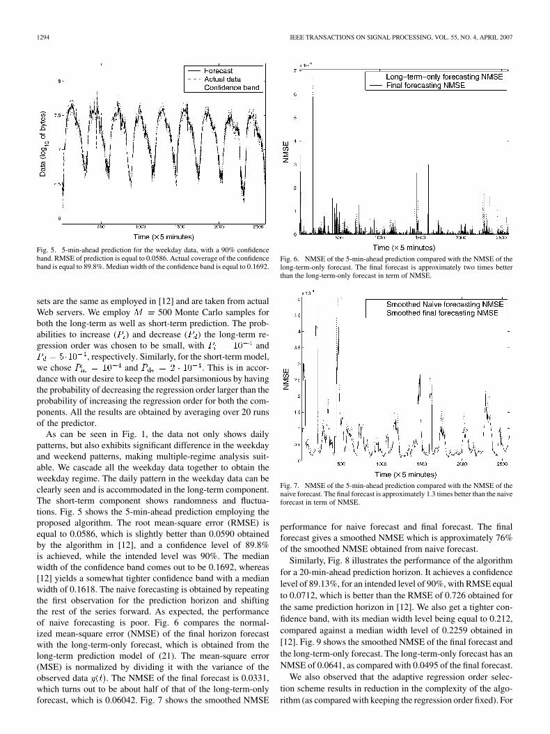
Fig. 5. 5-min-ahead prediction for the weekday data, with a 90% confidenceband. RMSE of prediction is equal to 0.0586. Actual coverage of the confidenceband is equal to 89.8%. Median width of the confidence band is equal to 0.1692.

sets are the same as employed in [12] and are taken from actualWeb servers. We employ 500 Monte Carlo samples forboth the long-term as well as short-term prediction. The prob-abilities to increase ( ) and decrease ( ) the long-term re-gression order was chosen to be small, with and

, respectively. Similarly, for the short-term model,we chose and . This is in accor-dance with our desire to keep the model parsimonious by havingthe probability of decreasing the regression order larger than theprobability of increasing the regression order for both the com-ponents. All the results are obtained by averaging over 20 runsof the predictor.

As can be seen in Fig. 1, the data not only shows dailypatterns, but also exhibits significant difference in the weekdayand weekend patterns, making multiple-regime analysis suit-able. We cascade all the weekday data together to obtain theweekday regime. The daily pattern in the weekday data can beclearly seen and is accommodated in the long-term component.The short-term component shows randomness and fluctua-tions. Fig. 5 shows the 5-min-ahead prediction employing theproposed algorithm. The root mean-square error (RMSE) isequal to 0.0586, which is slightly better than 0.0590 obtainedby the algorithm in [12], and a confidence level of 89.8%is achieved, while the intended level was 90%. The medianwidth of the confidence band comes out to be 0.1692, whereas[12] yields a somewhat tighter confidence band with a medianwidth of 0.1618. The naive forecasting is obtained by repeatingthe first observation for the prediction horizon and shiftingthe rest of the series forward. As expected, the performanceof naive forecasting is poor. Fig. 6 compares the normal-ized mean-square error (NMSE) of the final horizon forecastwith the long-term-only forecast, which is obtained from thelong-term prediction model of (21). The mean-square error(MSE) is normalized by dividing it with the variance of theobserved data . The NMSE of the final forecast is 0.0331,which turns out to be about half of that of the long-term-onlyforecast, which is 0.06042. Fig. 7 shows the smoothed NMSE

Fig. 6. NMSE of the 5-min-ahead prediction compared with the NMSE of thelong-term-only forecast. The final forecast is approximately two times betterthan the long-term-only forecast in term of NMSE.

Fig. 7. NMSE of the 5-min-ahead prediction compared with the NMSE of thenaive forecast. The final forecast is approximately 1.3 times better than the naiveforecast in term of NMSE.

performance for naive forecast and final forecast. The finalforecast gives a smoothed NMSE which is approximately 76%of the smoothed NMSE obtained from naive forecast.

Similarly, Fig. 8 illustrates the performance of the algorithmfor a 20-min-ahead prediction horizon. It achieves a confidencelevel of 89.13%, for an intended level of 90%, with RMSE equalto 0.0712, which is better than the RMSE of 0.726 obtained forthe same prediction horizon in [12]. We also get a tighter con-fidence band, with its median width level being equal to 0.212,compared against a median width level of 0.2259 obtained in[12]. Fig. 9 shows the smoothed NMSE of the final forecast andthe long-term-only forecast. The long-term-only forecast has anNMSE of 0.0641, as compared with 0.0495 of the final forecast.

We also observed that the adaptive regression order selec-tion scheme results in reduction in the complexity of the algo-rithm (as compared with keeping the regression order fixed). For


Fig. 8. 20-min-ahead prediction for the weekday data, with a 90% confidenceband. RMSE of prediction is equal to 0.0712. Actual coverage of the confidenceband is equal to 89.13%. Median width of the confidence band is equal to 0.212.

Fig. 9. Smoothed NMSE of the 20-min-ahead prediction compared with thesmoothed NMSE of the long-term-only forecast. The final forecast is approxi-mately 1.3 times better than the long-term-only forecast in term of NMSE.

the short-term component, the average regression order comesout to be approximately 4 for the 5-min-ahead as well as the20-min-ahead prediction, while at the same time, we could actu-ally have the regression order up to 8, allowing better modeling.Similarly, the average order of the harmonic regression comesout to be approximately 6 for the 5-min-ahead prediction, andaround 7.6 for the 20-min-ahead prediction, which is well below11, and way below the original 288. This shows that the adap-tive selection of regression order indeed reduces the complexityof the algorithm and makes it suitable for applications involvingfast learning and real-time prediction.

To demonstrate the advantage of selecting the basis subsetadaptively at each instant from a set of high energy and highcoherence waves over keeping the basis set fixed, we ran thealgorithm for a 5-min-ahead prediction with a fixed harmonic

Fig. 10. Another example at a different commercial website. 5-min-ahead pre-diction for the weekday data, with a 90% confidence band. RMSE of predictionis equal to 0.0439. Actual coverage of the confidence band is equal to 89.7%.Median width of the confidence band is equal to 0.1182.

regression of order 41 (first 20 sines, first 20 cosines, and theDC (zero-frequency) component) for the long-term model, andsuppressed the order-changing moves; the rest of the parametersremaining same. The RMSE for the 5-min-ahead prediction inthis setting turned out to be 0.0593, which is slightly worse than0.0586, which was obtained with adaptive order selection. Thisclearly implies that any improvement in accuracy by employinga larger (and fixed) number of harmonics is more than compen-sated by the estimation errors in the value of the coefficients.Thus, it is better to have a smaller basis set with harmonics thatcontribute significantly to the model (which we determine onthe basis of the energy and the coherence values).

Moreover, the algorithm is quite robust to the parametervalues, and different values of the order-changing parameters( and ), and different initial regression order forboth the long-term as well as short-term model donot affect the performance of the algorithm significantly.

Fig. 10 shows simulations on another set of data from a dif-ferent commercial website, which also shows the superior per-formance of the proposed algorithm over that of [12]. For a5-min-ahead prediction, we obtain an RMSE of 0.0439 with theactual convergence of the confidence band equal to 89.7%, andmedian width 0.1292. On the other hand, for the same data, thealgorithm in [12] (Fig. 15) yields an RMSE of 0.0464 and theactual confidence band coverage equal to 86%, although the me-dian width is slightly better there at 0.1132 as compared with0.1182 of the proposed algorithm.

VI. CONCLUSION

We have proposed a novel scheme for the forecasting ofa Web server workload time series which exhibits strongperiodic patterns. A hierarchical framework is used to sepa-rately predict the long-term and the short-term components.Separating the time series into two components reduces the


data history required to train model, thereby reducing theimpact of changes in the trend process. The long-term forecastis performed using dynamic harmonic regression, while theresidual short-term component is tracked as an autoregressiveprocess. The coefficients of both processes are tracked under astochastic state-space setting, and the order of both regressionsare adaptively selected by the SMC technique via resampling.Also, the predictions yield simultaneous confidence bands,which can be used to support probability-based service-levelagreements and for optimal resource allocation. Simulationresults also show that the algorithm is quite robust to the modelparameters. Modeling the noise in the short-term model by aheavy-tailed distribution makes the algorithm robust to outliersin the data. Furthermore, the proposed model has the capabilityto automatically handle nonstationarity in both the long-termas well as the short-term data as it allows the model parametersto change with time.

REFERENCES

[1] V. A. F. Almeida and D. A. Menasce, Capacity Planning for Web Ser-vices: Metrics, Models, and Methods. Englewood Cliffs, NJ: Pren-tice-Hall, 2002.

[2] A. Chandra, W. Gong, and P. Shenoy, “Dynamic resource allocationfor shared data centers using online measurements,” in Proc. 2003 ACMJoint Int. Conf. Measurement Modeling of Computer Systems (SIG-METRICS’03), Jun. 2003, vol. 31, pp. 300–301.

[3] R. P. Doyle, J. S. Chase, O. M. Asad, W. Jen, and A. M. Vahdat,“Model-based resource provisioning in a Web service utility,” in Proc.2003 USENIX Symp. Internet Technologies Systems, Seattle, WA, Mar.26-28, 2003.

[4] D. P. De Farias, A. King, M. Squillante, and B. Van Roy, “Dynamiccontrol of Web server farms,” in Proc. 2002 INFORMS Revenue Man-agement Section Conf., New York, Jun. 13-14, 2002.

[5] D. P. Pazel, T. Eilam, L. L. Fong, M. Kalantar, K. Appleby, and G.Goldszmidt, “Neptune: A dynamic resource allocation and planningsystem for a cluster computing utility,” in Proc. 2002 IEEE/ACM Int.Symp. Cluster Computing Grid, May 2002, pp. 48–55.

[6] M. E. Crovella and A. Bestavros, “Self-similarity in world wide Webtraffic: Evidence and possible causes,” in Proc. 2002 IEEE/ACM Int.Symp. Cluster Computing Grid, Dec. 1997, vol. 5, pp. 835–846.

[7] J. R. Gallardo, D. Makrakis, and M. Angulo, “Dynamic resource man-agement considering the real behavior of the aggregate traffic,” IEEETrans. Multimedia, vol. 3, no. 2, pp. 177–185, June 2001.

[8] K. Kant and Y. Won, “Server capacity planning for Web traffic work-load,” IEEE Trans. Knowl. Data Eng., vol. 11, no. 5, pp. 731–747,1999.

[9] M. Arlitt and C. L. Williamson, “Internet Web servers: Workload char-acterization and performance implications,” IEEE Trans. Netw., vol. 5,no. 5, pp. 631–645, 1997.

[10] M. S. Squillante, D. D. Yao, and L. Zhang, “Web traffic modellingand Web server performance analysis,” in Proc. 1999 Conf. DecisionControl, Dec. 1999, pp. 4432–4439.

[11] D. Shen and J. L. Hellerstein, “Predictive models for proactive networkmanagement: Application to a production Web server,” in Proc. 2000IEEE/IFIP Network Operations Management Symp., Apr. 2000, pp.833–846.

[12] T. H. Li, “A hierarchical framework for modeling and forecasting Webserver workload,” J. Amer. Stat. Assoc., vol. 100, no. 471, pp. 748–763,Sep. 2005.

[13] P. C. Young, D. J. Pedregal, and W. Tych, “Dynamic harmonic regres-sion,” J. Forecast., vol. 18, pp. 369–394, 1999.

[14] T. H. Li and M. J. Hinich, “A filter bank approach for modeling andforecasting seasonal patterns,” Technometrics, vol. 44, no. 1, pp. 1–14,2002.

[15] R. Chen and J. S. Liu, “Sequential Monte Carlo methods for dynamicsystems,” J. Amer. Stat. Assoc., vol. 93, pp. 1302–1044, 1998.

[16] X. Wang, R. Chen, and J. S. Liu, “Monte Carlo Bayesian signal pro-cessing for wireless communications,” J. VLSI Signal Process., vol. 30,no. 1–3, pp. 89–105, Jan.–Feb.–Mar. 2002.

[17] R. Chen, X. Wang, and J. S. Liu, “Adaptive joint detection and decodingin flat-fading channels via mixture Kalman filtering,” IEEE Trans. Inf.Theory, vol. 46, no. 6, pp. 2079–2094, Sep. 2000.

[18] C. Andrieu, M. Davy, and A. Doucet, “Efficient particle filtering forjump Markov systems—Applications to time-varying autoregres-sions,” IEEE Trans. Signal Process., vol. 51, no. 7, pp. 1762–1770,Jul. 2003.

[19] A. C. Harvey, Time Series Models, 4th ed. New York: HarvesterWheatsheaf, 1993.

[20] G. Gross and F. D. Galiana, “Short-term load forecasting,” IEEE Proc.,vol. 75, no. 12, pp. 1558–1573, Dec. 1987.

[21] I. Moghram and S. Rahman, “Analysis and evaluation of five short-term load forecasting techniques,” IEEE Trans. Power Sys., vol. 4, no.4, pp. 1484–1491, Oct. 1987.

[22] F. J. Nogales, J. Contreras, A. J. Conejo, and R. Espinola, “Forecastingnext-day electricity prices by time-series models,” IEEE Trans. PowerSys., vol. 17, no. 2, pp. 342–348, May 2002.

[23] D. C. Montgomery and E. A. Peck, Introduction to Linear RegressionAnalysis. New York: Wiley, 1992.

[24] D. Guo, X. Wang, and R. Chen, “Wavelet-based sequential MonteCarlo blind receivers in fading channels with unknown channel statis-tics,” IEEE Trans. Signal Process., vol. 52, no. 1, pp. 227–239, Jan.2004.

[25] A. Doucet, S. J. Godsill, and C. Andrieu, “On sequential Monte Carlosampling methods for Bayesian filtering,” Stat. Comp., vol. 10, no. 3,pp. 197–208, 2000.

[26] A. Doucet and C. Andrieu, “Iterative algorithms for state estimationof jump Markov linear systems,” IEEE Trans. Signal Process., vol. 49,no. 6, pp. 1216–1227, Jun. 2001.

[27] R. Chen and J. S. Liu, “Mixture Kalman filters,” J. Amer. Stat. Assoc.(B), vol. 62, pp. 493–509, 2000.

[28] R. Prado, G. Huerta, and M. West, “Bayesian time-varying autoregres-sions: Theory, methods and applications,” J. Inst. Math. Statist. Univ.Sao Paolo, no. 4, pp. 405–422, 2000.

[29] R. Prado and G. Huerta, “Time-varying autoregression with modelorder uncertainty,” J. Time Series Anal., vol. 23, no. 5, pp. 599–618,2002.

Tom Vercauteren graduated from Ecole Polytech-nique, Paris, France, in 2003 and received the M.S.degree in the Department of Electrical Engineering,Columbia University, New York, in 2004. He is cur-rently working towards the Ph.D. degree in INRIA,Sophia-Antipolis, France.

His research interests are in the area of statisticalsignal processing.

Pradeep Aggarwal received the B.Tech. degree inelectrical engineering from the Indian Institute ofTechnology—Bombay, India, in 2004 and the M.S.degree in electrical engineering from Columbia Uni-versity, New York, in 2006. He is currently workingtowards the Ph.D. degree in electrical engineering atColumbia University.

His research interests are in the area of communi-cations and statistical signal processing.


Xiaodong Wang (S’98–M’98–SM’04) received thePh.D. degree in electrical engineering from PrincetonUniversity, Princeton, NJ.

Currently, he is on the faculty of the Department ofElectrical Engineering, Columbia University. His re-search interests fall in the general areas of computing,signal processing, and communications, and he haspublished extensively in these areas. Among his pub-lications is a recent book entitled Wireless Communi-cation Systems: Advanced Techniques for Signal Re-ception (Englewood Cliffs, NJ: Prentice-Hall, 2003).

His current research interests include wireless communications, statistical signalprocessing, and genomic signal processing.

Dr. Wang received the 1999 NSF CAREER Award and the 2001 IEEECommunications Society and Information Theory Society Joint Paper Award.He currently serves as an Associate Editor for the IEEE TRANSACTIONS ON

COMMUNICATIONS, the IEEE TRANSACTIONS ON WIRELESS COMMUNICATIONS,the IEEE TRANSACTIONS ON SIGNAL PROCESSING, and the IEEE TRANSACTIONS

ON INFORMATION THEORY.

Ta-Hsin Li (S’89–M’92–SM’04) received the M.S.degree in electrical engineering from Tsinghua Uni-versity, Beijing, China, in 1984 and the Ph.D. degreein applied mathematics from the University of Mary-land, College Park, in 1992.

From 1992 to 1998, he taught at Texas A&MUniversity, College Station, and the Universityof California, Santa Barbara, as an Assistant andAssociate Professor of statistics. Since 1999, he hasbeen with the IBM T. J. Watson Research Center,Yorktown Heights, NY. He also serves as Adjunct

Professor at the Electrical Engineering Department of Columbia University,New York. His current research interests include time-series analysis, spectraland wavelet analysis, and statistical signal processing.

Dr. Li is a Fellow of the American Statistical Association (ASA). He currentlyserves as Associate Editor for the IEEE TRANSACTIONS ON SIGNAL PROCESSING

and for the EURASIP Journal on Applied Signal Processing.

hierarchical forecasting of web server workload using sequential monte ... · hierarchical...

Documents