Hierarchical linear-nonlinear cascade models of dendriticintegration

DJ Strouse

Computational and Biological Learning LaboratoryDepartment of Engineering

Churchill CollegeUniversity of Cambridge

This dissertation is submitted for the degree of Master of Philosophy.

For creating a stimulating and fun place to work and learn, I would like to thank the faculty andstudents at CBL. In particular, I would like to thank Cristina Savin for making me a more criticalscientist and drinker of wine, Rich Turner for making me a more careful scientist, Peter Orbanz for hisgenerosity and patience in sharing his mathematical wisdom, and Emil Hewage, Ferenc Huszár, DianaBurk, Koa Heaukulani, and Dan Roy for the banter.

I would also like to thank Peter Dayan, Peter Latham, Maneesh Sahani, and the rest of the Gatsbyfor providing a “home away from home” in London, Maneesh Sahani and Zoubin Ghahramani forserving as my examiners, Peter Patrikis and the Churchill Foundation for their support, financial andotherwise, and Maneesh Sahani, Jonathan Pillow, Peter Dayan, Peter Latham, Yee Whye Teh, MarkGoldman, Matthias Bethge, Jeremy Freeman, and Eero Simoncelli for useful discussions.

Most importantly, I have had the great fortune of working on interesting problems with individualswho are both talented collaborators and good friends. I would like to thank Tiago Branco for intro-ducing me to the messy world of experimental neuroscience and Judit Makara and Michael Häusserfor having the patience to talk biology with a physicist. Finally, I would like to thank my advisorMáté Lengyel for his generosity, for providing an endless supply of ideas and criticism, and for makingme a more critical scientist, Balázs Ujfalussy for always providing a sounding board for new ideas,for cheerfully weathering our comedy of errors, and for performing all of the compartmental modelsimulations, and to both of them for keeping science fun.

This dissertation is the result of my own work and includes nothing which is the outcome of workdone in collaboration except where specifically indicated in the text.

1

Abstract

Accumulating experimental evidence suggests that nonlinear dendritic processing plays a crucial role insingle-neuron information processing. Yet, while experimental methods have progressed to the pointof enabling precise spatial and temporal stimulation of the dendritic tree, there currently exists nosimple, canonical model for dendritic computation. Borrowing inspiration from the recent success andpopularity of linear-nonlinear-Poisson (LNP) and generalized linear models (GLMs) for sensory neuralcoding, we here develop a hierarchical linear-nonlinear (hLN) cascade model for dendritic integrationwhich is analytically tractable, interpretable, and can be fit to arbitrarily complex dendritic trees.

Contents

1 Introduction 1

2 Hierarchical linear-nonlinear cascade models 32.1 Background . . . . . . . . . . . . . . . . . . . . . . . . . . . . . . . . . . . . . . . . . . . 32.2 Formal definition of the hLN model for dendritic computation . . . . . . . . . . . . . . . 42.3 Parameter estimation: overview . . . . . . . . . . . . . . . . . . . . . . . . . . . . . . . . 52.4 Parameter estimation: initialization . . . . . . . . . . . . . . . . . . . . . . . . . . . . . 62.5 Parameter estimation: optimization details . . . . . . . . . . . . . . . . . . . . . . . . . 6

3 Validation of fitting 8

4 Validation of model selection 12

5 Fitting compartmental model simulation data 145.1 Experiment 1: clustered vs. distributed synapses, 20Hz inputs . . . . . . . . . . . . . . . 155.2 Experiment 2: clustered vs. distributed synapses, 2Hz inputs . . . . . . . . . . . . . . . 175.3 Experiment 3: two branches, within- and across-branch synchronization . . . . . . . . . 175.4 Experiment 4: two branches, with active conductances . . . . . . . . . . . . . . . . . . . 19

6 Discussion 246.1 Improving parameter estimation . . . . . . . . . . . . . . . . . . . . . . . . . . . . . . . 24

6.1.1 Structure learning . . . . . . . . . . . . . . . . . . . . . . . . . . . . . . . . . . . 246.1.2 Active learning . . . . . . . . . . . . . . . . . . . . . . . . . . . . . . . . . . . . . 246.1.3 Sparsity-inducing regularization of synaptic kernel basis weights . . . . . . . . . 246.1.4 Alternative objective functions . . . . . . . . . . . . . . . . . . . . . . . . . . . . 25

6.2 Expanding the model class . . . . . . . . . . . . . . . . . . . . . . . . . . . . . . . . . . . 256.2.1 Alternative basis functions . . . . . . . . . . . . . . . . . . . . . . . . . . . . . . 256.2.2 Alternative noise models . . . . . . . . . . . . . . . . . . . . . . . . . . . . . . . . 256.2.3 Additional nonlinearities . . . . . . . . . . . . . . . . . . . . . . . . . . . . . . . . 256.2.4 Output feedback filter . . . . . . . . . . . . . . . . . . . . . . . . . . . . . . . . . 266.2.5 Latent variable models . . . . . . . . . . . . . . . . . . . . . . . . . . . . . . . . . 26

6.3 Additional experiments . . . . . . . . . . . . . . . . . . . . . . . . . . . . . . . . . . . . 266.3.1 Natural synaptic inputs . . . . . . . . . . . . . . . . . . . . . . . . . . . . . . . . 266.3.2 Experiments with real neurons . . . . . . . . . . . . . . . . . . . . . . . . . . . . 26

7 Conclusions 27

2

Chapter 1

Introduction

How single cells process information is a central question in computational neuroscience. Most compu-tational models for single cells (e.g. integrate-and-fire [Izhikevich 2003], spike response models [Gerstnerand Kistler 2002]) implicitly ignore the intricate geometry of a neuron’s dendritic tree, treating themas “point neurons.” Typically, this is done by assuming that synaptic inputs are linearly summed andpassed through a single global nonlinearity (e.g. a spike-generating mechanism). By doing so, thelocations of synapses are ignored, and it is assumed that any local processing in the dendritic tree(i.e. nonlinear interactions between subsets of synaptic inputs) is insignificant [Gerstner and Kistler2002, Dayan and Abbott 2001]. From this viewpoint, it is the single cell that is the fundamentalcomputational unit of the brain [Zador 2000].

However, accumulating experimental evidence over the last two decades speaks to the contrary.Spurred by methodological developments granting researchers precise spatial and temporal control overthe inputs to single cells, including glutamate uncaging and focal stimulation, a series of experimentshave demonstrated both spatial [Magee 2000,Schiller et al 2000,Polsky et al 2004,London and Häusser2005, Losonczy and Magee 2006, Spruston 2008] and temporal [Branco et al 2010] nonlinearities indendritic processing. Together, these results suggest that local dendritic processing is not insignificantand that the dendritic “subunit” [Poirazi et al 2003a,Poirazi et al 2003b,Polsky et al 2004], not singlecells, may be the fundamental computational unit of the brain [Branco et al 2010].

Despite these experimental advances, there still exists no simple, canonical formalization of den-dritic computation. At one extreme, multi-compartmental models retain as much biophysical detail aspossible, modeling a cell down to the mechanics of membrane channels and propagation of electricalsignals. While such models are expressive enough to exhibit the spatial and temporal dendritic nonlin-earities discovered in experiments, they are both difficult to fit to experimental data [Huys et al 2006]and to analyze mathematically. Moreover, by focusing on biophysics, rather than the functional map-ping from inputs to outputs, they are difficult to interpret from a computational perspective. At theopposite extreme, heuristic “two-layer network” models [Poirazi et al 2003a,Poirazi et al 2003b,Polskyet al 2004], which assume that the somatic membrane potential is produced by passing the instanta-neous synaptic inputs through a two-layer linear-nonlinear cascade, are easy to analyze mathematicallyand interpret computationally. However, these models were designed to work only with static inputsand outputs, restricting their experimental application to artificial stimulus protocols involving brief,intense stimulation, rather than extended spike trains with realistic statistical properties. Moreover,because of the restriction to static inputs and outputs, the metrics for judging nonlinear dendriticbehavior were based only on either (1) instantaneous firing rates or (2) peaks or means of somaticmembrane potential, rather than predictiveness of dynamically changing firing rates or full membranepotential traces.

We propose here a model class which retains the simplicity and interpretability of the two-layernetwork but which can also (1) handle dynamic inputs, (2) model dendritic trees of arbitrary complex-ity (using a hierarchical linear-nonlinear cascade), (3) be efficiently fit directly to existing experimental

1

...

...

......

......

...

temporal filterlinearnonlinear additive noise

input synapses dendritic tree

soma

...

1L

...

1N

...

2L

...

......

...

output

0 10020 40 60 80time (ms)

basis functions

Figure 1.1: Pictoral representation of the hLN model. Spike train inputs are passed throughtemporal filters (representing synapses), followed by a hierarchy of LN cascades (representing den-drites), and a final linear or LN step (representing the soma), along with the addition of additivewhite Gaussian noise, to produce a somatic membrane potential. Example models at far right are aone-layer linear model (1L), one-layer nonlinear model (1N), and a two-layer linear model (2L); thelarger example model at left is a three-layer nonlinear (3N) model. Basis functions at the bottom wereproduced according to eqn 2.4 with M = 10, a = 3.75, and c = .01. The horizontal axis shows timeflowing into the past. Note the increased temporal resolution for more recent times. Note also that, forsimplicity, the tree (hierarchy) is depicted as uniformly deep and that synapses are depicted as beingconnected to only the deepest subunits, but that in general, the tree may be of nonuniform depth andthat synapses may be connected to any subunit (including the root subunit representing the soma).Figure credit: Balázs Ujfalussy.

data, and (4) be judged by its predictiveness of full somatic membrane potential traces. More specif-ically, the hLN model is aimed at experiments in which a number of synapses are stimulated in anarbitrarily complex spatiotemporal pattern while the somatic membrane potential of the cell is simul-taneously recorded, and it is this mapping from input spike trains to membrane potential trace that weseek to learn (figure 1.1). Importantly, this model allows us to identify the appropriate computationalsubunits of neurons in a statistically principled, data-driven way using more natural input spike trains.

In the next chapter, we introduce the hierarchical linear-nonlinear cascade model for dendriticcomputation and describe how to fit it to experimental data. We then demonstrate the success ofour fitting procedure using synthetic data for which the ground-truth parameters are known. Next,in order to gain confidence in our ability to make conclusive statements about nonlinear dendriticprocessing in real cells, we demonstrate the model’s ability to distinguish data generated from linear,nonlinear, and two-layer networks though model selection. Having verified these basic properties of thehLN model, we next demonstrate its biological relevance by fitting data generated from biophysicallyrealistic multi-compartmental models. Through a series of compartmental model experiments, wedemonstrate how the nonlinear dendritic properties discovered depend on the stimulation protocoland synapse locations. Finally, we close by highlighting shortcomings of the current version of themodel and directions for future work.

2

Chapter 2

Hierarchical linear-nonlinear cascademodels

2.1 BackgroundLinear-nonlinear (LN) cascade models have gained popularity in the neural coding literature over thelast decade as models for the spiking responses of sensory-driven neurons [Schwartz et al 2006,Pillow2007, Pillow et al 2008]. In these cases, since the goal is to predict spikes, the LN cascade producesa firing rate which is then fed into a Poisson spike generation process, yielding a linear-nonlinear-Poisson (LNP) model. The LNP model is a special case of a more general class of models calledgeneralized linear models (GLMs), which includes any probabilistic model with a random variableoutput distributed according to an exponential family distribution whose mean is produced by passinga linear combination of its inputs through a global nonlinearity [Truccolo et al 2005,Pillow 2007,Pillowet al 2008]. More recently, hierarchical LN (hLN) cascade models have been proposed as models forthe multiple layers of processing that occur in sensory circuits [Freeman et al 2012,Vintch et al 2012].

Inspired by the success of GLMs and seeking to leverage a growing body of theoretical and empiricalresults regarding them, we propose that hLN models may be used to model dendritic processing as well.There is however an important difference between our use of these models and their typical use in theneural coding literature. In that literature, the primary model inputs are (continuous) sensory signals(such as pixel intensities) while the model outputs are (binary) spike trains. In our own application,this pattern is reversed - the model inputs are (binary) spike trains (from presynaptic cells) and themodel outputs are the (continuous) somatic membrane potential of the cell. For this reason, we replacethe final Poisson spike generation stage with an additive white Gaussian noise model and include atemporal filter for each input line to model the excitatory postsynaptic potentials (EPSPs).1 In doingso, we specify a probabilistic model which can then be fit to experimental data using standard methodsfrom statistics and machine learning. In the present case, we fit the model using maximum likelihoodvia coordinate ascent. A pictoral representation of the model is included in figure 1.1. We now describethe hLN model and our fitting procedure more formally.

1This comparison is a slight oversimplification - when feedback or cross-coupling filters are included, the GLM doesalso take binary spike train inputs. Indeed, it is from that application that we borrow tricks for handling the binaryinputs to the hLN model.

3

2.2 Formal definition of the hLN model for dendritic computa-tion

We will denote2 the input spike train to a cell by the (binary) T ×Nsyn matrix X, where T∆t is thelength of the experiment, time has been discretized into bins of size ∆t, and Nsyn is the number ofsynapses stimulated. We use a value of ∆t = 1 ms since this is a typical timescale of variation in spikingand somatic membrane potential. We assume that the response of the cell at time t depends only onits inputs over a recent, finite temporal window [t− τ, t] of length τ ; we use a value of τ = 150ms sincetypical EPSP decay times are shorter. For each synapse i,3 we then define the T × τ (binary) synapticinput matrix Xi such that row t of Xi (denoted by xi(t)) constitutes the most recent τ ms of spikeinputs to synapse i as of time t. The response of LN subunit j at time t in our hierarchical model isthen defined as:

rj(t) = gj

∑k∈csub(j)

wkrk(t) +∑

i∈csyn(j)

kTi xi(t) ;θj

, (2.1)

where gj is the nonlinearity for subunit j (parameterized by the vector θj), csub(j) denotes the set ofindices for the “children” of subunit j (that is, the set of subunits whose outputs are among the inputsto subunit j), csyn(j) denotes the set of indices for the synapses connected to subunit j, wk denotesthe weight on the output of subunit k, and ki is a τ -length vector representing the temporal filter,or time-inverted EPSP, of synapse i. The inputs to subunit j thus consist of two separate terms - aweighted summation of other subunit responses (the first term in eqn 2.1) and linearly filtered versionsof the subunit’s recent synaptic inputs (the second term in eqn 2.1). In more biological parlance,the first term represents the influence of subbranchlet stimulation on dendritic branchlet j and thesecond term represents the influence of EPSPs for synapses on that branchlet. Note that the apparentrecursiveness of eqn 2.1 (i.e. that subunit responses appear on both sides of the equation) is onlyillusory since the hierarchy on subunits (implicitly defined by csub(j)) imposes that the inputs to asubunit will not depend on its own output. In other words, the subunits are arranged in a (directed)tree (figure 1.1).

Letting the “root” subunit in the hierarchy be indexed by the subscript j = 1, we then model thesomatic membrane potential at time t as:

v(t) =w1r1(t) + v0 + η(t) (2.2)=v(t) + η(t) (2.3)

where v0 is the baseline membrane potential (or offset, or bias), η(t) ∼ N(0, σ2

)represents additive

white Gaussian noise (of mean 0 and variance σ2), v(t) ≡ w1r1(t) + v0 is the noiseless predictedmembrane potential, and w1 is the output gain which defines the scale of variations in the predictedsomatic membrane potential.4

Throughout the work discussed here, we use a sigmoid (or logistic function) for the nonlinearity forall internal (i.e. non-root) subunits, defined by g(x;x0) = 1

1+e−(x+x0) , which takes an argument x andis parameterized by an input bias x0. For the root subunit, we use either this sigmoid or the identityfunction g(x) = x and henceforth refer to those models as having either nonlinear (N) or linear (L)

2Throughout this document, we will use bold uppercase letters such as X to denote matrices, bold lowercase letterssuch as x to denote vectors, and xT to denote the transpose of the vector x.

3We will use the convention that i indexes synapses (meant to connote “inputs”), j and k index LN subunits, and mindexes basis functions (to be introduced below).

4We use the standard conventions that ∼ means “distributed according to”, N (µ,Σ) denotes a multivariate Gaussiandistribution with mean µ and covariance matrix Σ, and N (x;µ,Σ) denotes the value of that distribution evaluated atx.

4

output, respectively. While typically a sigmoid would also be parameterized by an output offset, aninput gain, and an output gain, we do not include them explicitly, since they would be redundant withthe input bias of the parent subunit (for subunits j 6= 1) or v0 (for the root subunit j = 1), a globalscale factor on the input subunit weights wk and synaptic kernels ki, and the subunit output weightwj , respectively. We chose to use a sigmoid for two reasons. First, the sigmoid has been proposedelsewhere as an appropriate dendritic nonlinearity [Poirazi et al 2003a,Poirazi et al 2003b,Polsky et al2004]. Second, under different parameter settings and input statistics, the sigmoid is flexible enoughto capture purely linear, sublinear, and superlinear behavior, as well as combinations thereof.

It is worth noting that we assume in the work discussed here that the hLN architecture is given inadvance, that is that one knows csub(j) and csyn(j) for all subunits. When fitting experimental datainvolving the stimulation of a small portion of the dendritic tree, one often can narrow down the possibleappropriate architectures to a handful. By fitting an hLN model with each of these architectures andcomparing their performances, it is possible to identify the computational subunits of a cell. Inchapter 5, we perform this analysis on experimental data produced from a multi-compartmental modelof a cortical pyramidal neuron. In section 6.1.1, we discuss the possibility of extending the hLN modelto learning the appropriate hiearchical model structure in a more principled and automatic way.

In order to (1) reduce the number of parameters that we must infer and (2) impose temporalsmoothness on the synaptic kernels, we represent ki in terms of a set of M basis functions (following[Pillow et al 2008]) of the form:

fm(t′) =

{12 cos(a log[t′ + c]− φm) + 1

2 t′ s.t. a log[t′ + c] ∈ [φm − π, φm + π]

0 otherwise, (2.4)

where t′ represents time flowing into the past and θm = mM . This family of basis functions is plotted in

the bottom of figure 1.1. In words, this family constitutes a series of cosine “bumps” with varying phasesin log-transformed time. We chose this set due to the property, suggested in [Pillow et al 2008], thatit allows for fine-grained temporal sensitivities for recent inputs while imposing more coarse-grainedtemporal sensitivities for less recent inputs. Throughout the work discussed here, we use M = 10,a = 3.75, and c = .01. These numbers were simply chosen to yield realistic timescales for the temporalsensitivities of synapses.

By convolving the rows of the synaptic input matrices Xi with this set of basis functions to createthe T ×M convolved synaptic input (or design) matrices Xi (with rows xi(t)), we can rewrite eqn 2.1as:

rj(t) = gj

∑k∈csub(j)

wkrk(t) +∑

i∈csyn(j)

bTi xi(t) ;θj

, (2.5)

where the only differences are that xi(t) has been replaced by xi(t) and the synaptic filter ki has beenreplaced with its basis weight representation denoted by theM -length vector bi. Note that this changereduces the number of synaptic parameters we need to estimate from Nsynτ to NsynM . For the valuesof these parameters we consider (Nsyn = 10 − 40, τ = 150, and M = 10), this constitutes a 15-foldreduction from 1500− 6000 to 100− 400 parameters.

2.3 Parameter estimation: overviewOur goal is to fit this model to experimental data in the form of the synaptic inputs Xi and simulta-neously recorded somatic membrane potential v (a T -length vector whose tth entry is the membranepotential at time t). A natural method for doing so is via maximum likelihood (ML), that is bymaximizing the conditional probability of v given the inputs Xi and model parameters. Due to our

5

assumption of additive white Gaussian noise, ML fitting is equivalent to choosing the parameterswhich minimize the squared training error (commonly referred to as the “least squared error”, or LSE,parameters). Concatenating the temporal history of our noiseless predicted membrane potential intothe T -length vector v, the Nsyn design matrices Xi into a single T × (NsynM) design matrix X, thesubunit output weights into an Nsub-length vector w, the Nsyn synaptic basis weight vectors bi into asingle NsynM -length vector b, and the Nsub nonlinearity parameter vectors θj into a single parametervector θ, we can write the log likelihood of the model parameters w, b, θ, v0, and σ2 as:

l(w,b,θ, v0, σ

2)

= logP(v | X,w,b,θ, v0, σ2

)(2.6)

= logN(v; v

(X,w,b,θ, v0

), σ21

). (2.7)

Unfortunately, unlike the ML problem for the LNP model used in neural coding [Paninski 2004],our ML problem is not convex, potentially making optimization more difficult, or even impractical,for our model. Fortunately, despite the nonconvexity, we found that maximization of eqn 2.7 viasubunit-wise coordinate ascent performed well (figures 3.2-3.3).

Intuitively, we begin by randomly initializing the model parameters w, b, θ, v0, and σ2 with“reasonable” values, then iterate over subunits j, maximizing eqn 2.7 with respect to wj , bj , θj , v0,and σ2 while keeping wk, bk, and θk fixed for k 6= j until convergence.

2.4 Parameter estimation: initializationFor “reasonable” initial parameters, we choose ones such that the subunit sigmoids are not saturatedduring the entire experiment. It is important to avoid that parameter regime because the derivativesof the log likelihood would then be very small, leading to very slow performance for coordinate ascent.More specifically, we initialize w, b, and θ and then rescale them such that for each sigmoidal subunit,the input mean and rms deviation about the mean are -1.5 and 2.5, respectively, which empiricallycorresponds to the “active”, unsaturated input regime. If the root (output) subunit (j = 1) waslinear, we fixed w1 = 1, since it is redundant with the wk and bi for k ∈ csub(1) and i ∈ csyn(1), andrescaled wk and bi so that the range (i.e. difference between maximum and minimum) of the predictedmembrane potential was 15mV.

Each element of the nonlinearity parameter vector θ was initialized to -6, though its initial valuewas not important since it was rescaled as described above anyways. For the non-root, or “internal”,subunits (j 6= 1), the subunit output weight wj was drawn uniformly from the interval [2, 3], while forthe root subunit (j = 1), w1 was drawn from the interval [13, 17]. Finally, the basis weights bi foreach synapse i were chosen to be sparse and such that the kernel ki was unimodal. Unimodality wasencouraged by selecting consecutive nonzero elements from 1:M, that is basis elements with similarmaxima (see eqn 2.4), and choosing their values so that one “primary” element was largest and elementsof increasing distance from the primary element had decreasing magnitudes. More specifically, we firstchoose the number of nonzero elements of bi from the integer interval [1, 3], select one element b(p)iat random as the “primary” element, draw that element from N (10, 2), draw the remaining nonzeroselements b(m)

i fromN (10α, 2α) where α = 12

|m−p|, and reset any nonzero elements with a value less than1 to have value 1. Essentially, this seemingly complex procedure is really just an ad-hoc method foravoiding parameter regimes with saturated sigmoids and therefore tiny derivatives of the log likelihood.

2.5 Parameter estimation: optimization detailsFor the coordinate optimization iteration order, we typically begin with the subunits furthest fromthe root (randomizing the order within a layer) and sweep through the tree towards the root, cyclingover all subunits several times until converence. The motivation for this ordering is that we optimize

6

the parameters of subunit j only after optimizing the parameters of all subunits k 6= j whose outputsconstitute the inputs to subunit j.

Maximization of eqn 2.7 for each iteration is performed via Matlab’s fmincon function with non-negativity constraints onw and σ and a non-positivity constraint on v0, using the trust-region-reflectivealgorithm - “a subspace trust-region method... based on the interior-reflective Newton method” (Matlabdocumentation). We placed the non-negativity constraint on w to eliminate a symmetry in the modelwhich involves flipping the sign of w and b and adjusting θ so that the input-output function ofthe model is unchanged but the sigmoids are activated “backwards” – that is, the sigmoids have highactivation at baseline, receive negative activation during synaptic stimulation, but due to a negativeoutput weight, the end result is still the same as normal. We used the trust-region-reflective algorithmbecause it was the recommended algorithm (Matlab documentation) for cases in which it was possibleto provide analytic derivatives (we could) and only bound or equality constraints were needed but notboth (we had only bounds).

We defined convergence of the coordinate optimization procedure using one of two conditions,whichever was met first: (1) two consecutive interations during which the log likelihood increased byless than 15 or (2) the completion of 20 iterations.

For coordinate optimization of a linear output subunit, it is possible to obtain closed-form solu-tions for the ML parameters. Thus for those optimization steps, we simply updated the parametersaccordingly.

We chose to use coordinate optimization, rather than optimizing all parameters at once, since (1)we avoid calculating the cross-subunit terms in the Hessian, (2) the Hessian we must store in memoryis orders of magnitude smaller, and (3) the individual coordinate optimization problems can be solvedreasonably rapidly. Moreover, coordinate optimization approaches (e.g. expectation-maximization, orEM) have been known to work well in many contexts. Most importantly, as we demonstrate in thenext chapter, this method works in practice in our own context.

5In retrospect, this is not a good choice of convergence condition since the meaning of the log likelihood changes withthe amount of data. Thus a more appropriate convergence condition would depend on the length of the experiment.

7

Chapter 3

Validation of fitting

Before applying the hLN model to experimental data sets, we validated our fitting procedure onsynthetic data sets produced from the hLN model. The purpose of doing so was to test our fittingprocedure in a setting in which (1) we knew the model was appropriate and (2) we knew the underlyingparameters of the model which generated the data and so could compare our inferred parameters withthe true ones. In this way, we could separate validation of the fitting procedure (here) from validationof the model’s biological relevance (see chapter 5).

More specifically, we generated data from the following models: (1) a single linear subunit (1L)with 10, 15, or 20 synapses, (2) a 2-layer, 3-subunit model with linear output (2L) and 10, 15, or 20total synapses divided between the two leaf subunits as 5 and 5, 5 and 10, or 10 and 10 synapses,respectively, (3) a 3-layer, 7-subunit model with linear output (3L) and 20, 25, 30, 35, or 40 totalsynapses divided between the four leaf subunits as 5 each, one with 10 and three with 5, two each with10 and 5, three with 10 and one with 5, and 10 each, respectively, and (4-6) the same models withoutput nonlinearities (1N, 2N, and 3N). The 1L, 1N, 2L, and 3N models are depicted in figure 1.1. Themotivation for varying the number of synapses was to test how the parameter estimation performanceand speed would scale to data sets of experimentally interesting sizes.

For the stimulation protocol, each synapse received an independent Poisson spike train with 10Hzfiring rate.

For each model, we generated 25 instantiations with different randomized parameters, generatedaccording to the procedure for optimization initialization described in section 2.4,1 for each of fourincreasing training data set sizes (1s, 2s, 4s, and 8s) and ran the estimation procedure described insections 2.3-2.5. The motivation for varying the training data set size was to test how much data mightbe required in later experiments using compartmental models or real cells.

The inferred models were then tested on a 4s test data set produced by the same model whichproduced the training data. We kept the size of the test data set constant (i.e. independent of thetraining data set size) because test performance variability would increase for smaller test data setsizes and we did not want to unfairly bias our test metrics against models training on smaller datasets. We measured performance both by the predictive power on the test data set (figure 3.2), as wellas by direct comparison of the inferred to true model parameters (3.3). We judged performance basedon the test set rather the training set in order to convince ourselves that “good” performance was notjust due to overfitting. This is especially important when doing model selection (chapter 4), sincea more complicated model can always achieve better training performance than a simpler one. Theexperimental protocol is summarized in figure 3.1.

The results are shown in figures 3.2 and 3.3. For the one-layer models, predictive performanceof the inferred model on the test data set approached that of the true model (i.e. the level limitedby noise) by the time the training data sets reached 2-4s. The parameter estimation performance

1The procedure was actually first developed for generating synthetic data sets and then borrowed for optimizationinitialization.

8

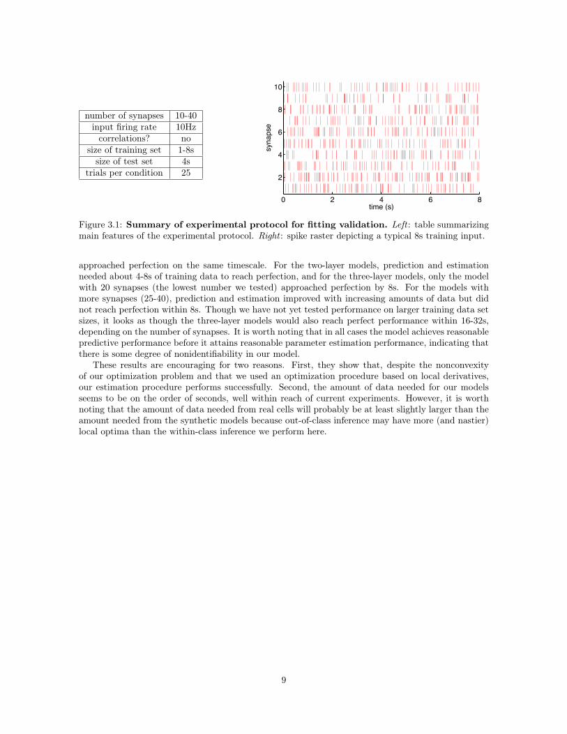
number of synapses 10-40input firing rate 10Hzcorrelations? no

size of training set 1-8ssize of test set 4s

trials per condition 25

time (s)

syna

pse

0 2 4 6 8

2

4

6

8

10

Figure 3.1: Summary of experimental protocol for fitting validation. Left : table summarizingmain features of the experimental protocol. Right : spike raster depicting a typical 8s training input.

approached perfection on the same timescale. For the two-layer models, prediction and estimationneeded about 4-8s of training data to reach perfection, and for the three-layer models, only the modelwith 20 synapses (the lowest number we tested) approached perfection by 8s. For the models withmore synapses (25-40), prediction and estimation improved with increasing amounts of data but didnot reach perfection within 8s. Though we have not yet tested performance on larger training data setsizes, it looks as though the three-layer models would also reach perfect performance within 16-32s,depending on the number of synapses. It is worth noting that in all cases the model achieves reasonablepredictive performance before it attains reasonable parameter estimation performance, indicating thatthere is some degree of nonidentifiability in our model.

These results are encouraging for two reasons. First, they show that, despite the nonconvexityof our optimization problem and that we used an optimization procedure based on local derivatives,our estimation procedure performs successfully. Second, the amount of data needed for our modelsseems to be on the order of seconds, well within reach of current experiments. However, it is worthnoting that the amount of data needed from real cells will probably be at least slightly larger than theamount needed from the synthetic models because out-of-class inference may have more (and nastier)local optima than the within-class inference we perform here.

9

one-layer models

linea

r out

put

nonl

inea

r out

put

two-layer models three-layer models

length of experiment (s)

fract

ion

test

sig

nal e

xpla

ined

1 2 4 80

0.2

0.4

0.6

0.8

1

time (ms)

v test

(mV)

0 100 200−65

−60

−55

−50truepredicted

length of experiment (s)

fract

ion

test

sig

nal e

xpla

ined

1 2 4 80

0.2

0.4

0.6

0.8

1

time (ms)

v test

(mV)

0 100 200−65

−60

−55

−50 truepredicted

length of experiment (s)

fract

ion

test

sig

nal e

xpla

ined

1 2 4 80

0.2

0.4

0.6

0.8

1

time (ms)v te

st (m

V)0 100 200

−65

−60

−55

−50 truepredicted

length of experiment (s)

fract

ion

test

sig

nal e

xpla

ined

1 2 4 80

0.2

0.4

0.6

0.8

1

length of experiment (s)

fract

ion

test

sig

nal e

xpla

ined

1 2 4 80

0.2

0.4

0.6

0.8

1 10 synapses15 synapses20 synapses25 synapses30 synapses35 synapses40 synapses

length of experiment (s)

fract

ion

test

sig

nal e

xpla

ined

1 2 4 80

0.2

0.4

0.6

0.8

1

Figure 3.2: Fitting validation. Predictive performance was measured by the fraction of the testsignal explained, defined as f = 1 − ε−σ

s where ε is the root-mean-square (rms) test set predictionerror, s is the standard deviation (s.d.) of the test somatic membrane potential, and σ is the noisestandard deviation. The horizontal axes show the amount of data in the training set (on a log scale)in seconds. Columns correspond to one-, two-, and three-layer models (from left to right) and rowscorrespond to models with linear (top) or nonlinear (bottom) root subunit. Lines of different colorscorrespond to different numbers of synapses (legend at top right). Circles indicate across-trial meansof f . Error bars are 95% confidence intervals across trials. Insets show example membrane potentialpredictions to provide intuition for intepreting our test metric. The predictions are from a random200ms interval of a trial with test performance indicated by the root of the black arrow and illustratepoor, reasonable, and excellent performance (counterclockwise from top left).

10

one-layer models

linea

r out

put

nonl

inea

r out

put

two-layer models three-layer models

length of experiment (s)

rms

erro

r

1 2 4 8

10−1

100

time (ms)

kern

el (m

V/sp

ike)

0 50 100 150−1

0

1

2truepredicted

length of experiment (s)

rms

erro

r

1 2 4 810−2

10−1

100

101

time (ms)

kern

el (m

V/sp

ike)

0 50 100 150−1

0

1

2truepredicted

length of experiment (s)

rms

erro

r

1 2 4 810−2

100

102

104

time (ms)

kern

el (m

V/sp

ike)

0 50 100 150−10

0

10

20truepredicted

length of experiment (s)

rms

erro

r

1 2 4 810−2

100

102

104

basis weights, b

frequ

ency

typical for multi−layer models

0 2 4 60

0.5

1

length of experiment (s)

rms

erro

r

1 2 4 810−2

100

102

104

10 synapses15 synapses20 synapses25 synapses30 synapses35 synapses40 synapses

basis weights, b

frequ

ency

typical for one−layer models

0 0.5 1 1.5 2 2.50

0.2

0.4

0.6

0.8

1

length of experiment (s)

rms

erro

r

1 2 4 810−2

100

102

104

Figure 3.3: Estimation validation. Estimation performance is shown only for the synaptic kernelbasis weights b, though estimation performance was similar or better for other model parameters.Estimation performance was measured by the rms error between the true and inferred basis weights.The horizontal axes show the amount of data in the training set (on a log scale) in seconds. Columnscorrespond to one-, two-, and three-layer models (from left to right) and rows correspond to modelswith linear (top) or nonlinear (bottom) root subunit. Lines of different colors correspond to differentnumbers of synapses (legend at top right). Circles indicate across-trial means. Error bars are 95%confidence intervals across trials. Two additional features are included to aid interpretation of themagnitude of rms errors. First, insets show example inferred kernels from a trial with estimationperformance indicated by the root of the black arrow. The predictions are meant to illustrate poor,reasonable, and excellent performance (clockwise from bottom right). Second, the histograms at rightillustrate typical distributions for the elements of b for one- (top) and multi-layer (bottom) models.

11

Chapter 4

Validation of model selection

Given that one of our goals is to make claims about the linear and nonlinear properties of real cells,we wanted to prove to ourselves that we could distinguish varying degrees of nonlinear behavior insynthetic models. If unsuccessful, this would seriously undermine our ability to distinguish betweendifferent models for real cells. If successful however, this would at least give us some confidence thatwe could identify varying degrees of nonlinear behavior under extended input trains with realisticstatistics.

To perform model selection, we use cross-validation on a test set, that is we choose the model withhighest predictive performance on a hold-out test set, as measured by the fraction test signal explained(see caption of figure 3.2 for definition). If two models perform equally well, we choose the simplermodel.

To test our model selection capabilities, we fit 1L, 1N, 2L, and 2N models to data generated fromeach model and checked to see whether our model selection procedure identified the correct underlyingmodel. Since we had already fit each of the four models to data generated from that same model inchapter 3, we needed only to fit the three remaining models to each data set. We concentrated only onthe 8s training data sets, since we were interested in model selection using adequate amounts of data.In each case, we fit all 25 trials for each of the 3 numbers of synapses simulated (10, 15, and 20). Forthe cases in which a two-layer model was fit to one-layer data, we randomly assigned 5 synapses eachto 2, 3, or 4 internal subunits, depending on the total of synapses; including the output subunit, therethen 3, 4, or 5 subunits total.

The results of our model selection experiment are shown in figure 4.1. Most importantly, in everycase, across models and number of synapses, our model selection procedure is successful in identifyingthe correct underlying model.

There are a couple features of figure 4.1 worth mentioning. To begin with, there is one case inwhich two models do equally well – for data from the 1L model, both the 1L and 1N models performessentially perfectly. This occurs because a sigmoidal subunit can easily imitate a linear relationshipby using small input weights (i.e. weights on subunits and synapses providing input to that subunit)and a bias which ensures the sigmoidal activation only receives small perturbations about its mostlinear regime (i.e. around zero activation). Indeed when we investigated the sigmoidal activation forthe 1N model fit to 1L data, the parameters w, b, and θ were set such that the 1N output sigmoidalwas perturbed only slightly about zero activation and thus imitated a 1L model.

Also, one might wonder why, in all cases besides the 1N model fit to 1L data, the models morecomplex than the underlying model do more poorly than the underlying model. Shouldn’t a 2L modelbe able to simulate a 1N model? And a 2N model a 2L model? There are at least two reasons why thisis not true in this case. First, we did not attempt to search the space of all possible synapse assignmentsand number of internal subunits, so it is possible that other model architectures than the ones we usedmight have allowed the more complex models to fare better. For example, assigning all synapses ina two-layer model to a single internal subunit whose output is the sole input to an output subunit

12

number of synapses

fract

ion

test

sig

nal e

xpla

ined

10 15 200

0.2

0.4

0.6

0.8

1

number of synapses

fract

ion

test

sig

nal e

xpla

ined

10 15 200

0.2

0.4

0.6

0.8

1

number of synapses

fract

ion

test

sig

nal e

xpla

ined

10 15 200

0.2

0.4

0.6

0.8

1

1L1N2L2N

number of synapses

fract

ion

test

sig

nal e

xpla

ined

10 15 200

0.2

0.4

0.6

0.8

1

linea

rno

nlin

ear

one-layer models two-layer models

Figure 4.1: Model selection validation. Model selection is carried out using cross-validation on atest set. Bars indicate the fraction of the test signal explained, as defined in the caption of figure 3.2.Columns correspond to data generated from one- (left) and two-layer (right) models and rows cor-respond to data generated from models with linear (top) or nonlinear (bottom) root subunit. Barsof different colors indicate the model being fit to data (legend at top right). Bar heights indicationacross-trial means. Error bars are 95% confidence intervals across trials.

would make it much easier to imitate a one-layer model. Second, it is possible that the more complex(i.e. two-layer) models simply did not have enough training data. While 8s was certainly enough datain our within-class validation experiments (see chapter 3 and the appropriate bars in figure 4.1), it ispossible that it was not enough data for out-of-class inference in the two-layer models. However, forthe purposes of validating our model selection procedure, we do not need to worry about these issues.In all cases in figure 4.1, the underlying model performed essentially perfectly, so improvements in theperformance of the more complicated models would not change the outcomes of our model selection.

13

Chapter 5

Fitting compartmental modelsimulation data

Assured that our fitting and model selection procedures were adequate, we next applied the hLNmodel to data from biophysically detailed multi-compartmental models. In particular, we set out toinvestigate (1) the computational subunits of cortical pyramidal neurons and (2) how the identificationof these subunits depends on the stimulation protocol used. These experiments were motivated by theobservation that many experiments investigating dendritic nonlinearities in real neurons use highlyartificial stimuli without necessarily mentioning the effect this may have on the resulting nonlinearityproperties identified. Indeed, the appropriateness of any input-output model of a nonlinear systemwill depend on the inputs used. For example, using small enough inputs to any (smooth) nonlinearsystem will make the input-output relationship appear linear.1

This investigation is further motivated by two recent studies. [Polsky et al 2004] noted that spatiallyand temporally clustered synaptic inputs lead to local nonlinearities in cortical pyramidal neurons,whereas inputs separated in either space (i.e. on different branches) or in time combine only linearly.However, as mentioned in chapter 1, that study used only paired inputs, rather than the extendedspike train inputs that cells would receive in vivo, and heuristic measures of nonlinearity (i.e. peakEPSP). [Gasparini and Magee 2006] performed a similar study in hippocampal CA1 pyramidal neuronsusing more temporally extended inputs and reached similar conclusions. Nevertheless, their nonlin-earity metrics were still heuristic (i.e. peak EPSP, firing rate, firing phase, occurrence of a dendriticspike), rather than based on model selection between input-output models predicting the full somaticmembrane potential trace (as can be done with the hLN model).

Building on [Polsky et al 2004] and [Gasparini and Magee 2006], we endeavored to demonstrate thedependence of identified dendritic nonlinearities on the spatial and temporal statistics of their synapticinputs using spike trains of more realistic timescales, as well as a more principled metric for judgingnonlinear behavior (i.e. model selection between increasingly complex hLN models).

In all cases, we used the cortical pyramidal neuron model with AMPA and NMDA synapses de-scribed in [Branco et al 2010]. In brief, the model includes a soma, an axon, 69 dendritic compartments,and the following active channels: Hodgkin-Huxley type Na+ and K+ channels, M-type K+ channel(slow, non-inactivating), Ca2+-dependent K+ channel, high-threshold Ca2+ current, and T-type Ca2+

channel. Simulations were all performed by Balázs Ujfalussy using the NEURON simulation environ-ment [Hines and Carnevale 1997].

In the first four experiments (sections 5.1-5.3), the active currents were not included in the modeland all nonlinear effects were mediated by either NMDA spikes (superlinear) or the reduction of thesynaptic driving force (sublinear) at large, synchronous inputs.

1This is the observation behind a common technique in applied mathematics for analyzing nonlinear systems called“linearization.”

14

5.1 Experiment 1: clustered vs. distributed synapses, 20Hzinputs

Our first experiment sought to demonstrate a simple point – that the identification of dendritic non-linearities would depend on both (1) synapse location and (2) correlations in the stimulus (i.e. inputspike trains). To do so, we stimulated 10 synapses that were either (a) clustered on a single basaldendrite or (b) distributed across 10 different branches. Our stimulus protocol was designed to allowparametric variation of correlations with fixed marginal statistics of r = 20Hz stimulation to eachsynapse. More specifically, the input spike train to each synapse consisted of two Poisson components:(1) an independent component with rate (1− α) r, where 0 ≤ α ≤ 1, and (2) a shared componentwith rate αr. While the independent component was private to each synapse (i.e. 10 different trainswere generated), the shared component was common to all synapses (i.e. only one was generated).Thus, α denotes the fraction of shared (synchronous) spikes, α = 0 corresponds to independent inputs,and α = 1 corresponds to synchronous inputs only. The spike train to each synapse then consistedof the sum of the independent and shared spike trains, thresholded to eliminate multiple spikes at asynapse in a single time bin.2 A small (1ms) jitter was added to the shared spikes. Each condition(i.e. clustered vs. distributed, value of α) was repeated for 10 trials, each with 16s of training dataand 4s of test data. The experimental protocol is summarized in figure 5.1.

The results of this experiment are shown in figure 5.2. For distributed synapses, the linear modelperforms very well regardless of input synchrony (left plot) and the nonlinear model offers little tono improvement (left and right plots). For clustered synapses, the situation is quite different. Whenthe inputs are independent (α = 0), the nonlinear model offers little improvement over the linearmodel (left and right). As input synchrony increases however, the linear model becomes progressivelyworse (left), while the nonlinear model maintains high performance (left), so that the nonlinear modelsperforms progressively better than the linear model (left and right). Across all levels of synchrony,prediction seems to be more difficult for the clustered case than for the distributed case, as both modelsperform significantly worse.

These results indicate that both the choice of synapse locations and stimulus statistics can play amajor role in the identification of dendritic nonlinearities. When synapses are chosen from throughoutthe dendritic tree, synaptic integration may appear linear, regardless of the stimulation protocol. Whensynapses are chosen from a tightly clustered group on a single branch, however, synaptic integrationmay appear linear for independent stimulation but nonlinear for correlated (synchronous) stimulation.Importantly, these results also suggest that the hLN model can capture quite well the behavior of adetailed biophysical compartmental model receiving extended inputs with varying statistics. Indeed,across all levels of synchrony, the best hLN model predicts about 90 or 95% of the test signal forclustered and distributed synapses, respectively.

However, upon closer examination of our results, we found an important caveat – the relativelystrong 20Hz stimulation which we applied in this experiment left all of the NMDA synapses in thedesensitized state (i.e. unresponsive to inputs) for virtually the entire duration of the experiment.Thus, the results of this experiment speak only to a passive dendritic tree. The reason we still foundnonlinear behavior under these conditions is due to the reduction of the synaptic driving force duringthe large, local depolarizations caused by the synchronous events.

2While this thresholding step does cause the marginal statistics and fraction of shared spikes to vary from thenumbers we intended, the deviations are neglible except for firing rates much larger than the ones we use. Specifically,the thresholding reduces both r and α by α (1− α) r2, where r is in spikes per ms, which even in the worst case scenario(i.e. α = 0.5) corresponds to errors of 1 part in 200 and 1 part in 5000 for r and α, respectively.

15

number of synapses 10location of synapses distributed or

clusteredinput firing rate 20Hzcorrelations? yes, parameterized

by αconductances passive only

(including NMDA)size of training set 16ssize of test set 4s

trials per condition 10time (s)

syna

pse

0 1 2 3 4

2

4

6

8

10

Figure 5.1: Clustered vs. distributed synapses, 20Hz inputs - summary of experimentalprotocol. Left : table summarizing main features of the experimental protocol. Right : spike rasterdepicting 4s of a typical training input with α = 0.4. Although we show results in figure 5.2 only forvalues of α up to 0.2, we use a higher value here for easier visualization of the shared spike events.

% shared spikes

fract

ion

test

sig

nal e

xpla

ined

0 1.25 2.5 5 10 200.7

0.75

0.8

0.85

0.9

0.95

1

% shared spikes

Δ fr

actio

n te

st s

igna

l exp

lain

ed (1

N−1

L)

0 1.25 2.5 5 10 20−0.05

0

0.05

0.1

0.15

0.2

linear nonlineardistributedclustered

Figure 5.2: Clustered vs. distributed synapses, 20Hz inputs - fitting results. Model perfor-mance was measured by the fraction of the test signal explained, defined as f∗ = 1− ε

s where ε is theroot-mean-square (rms) test set prediction error and s is the s.d. of the test signal (i.e. the test setsomatic membrane potential). This definition differs from that of f in the caption to figure 3.2 becausein this case we do not know the true level of noise. The horizontal axes show the fraction of sharedspikes α in percentage (on a log scale). The left plot shows f∗ for the 1L (linear) and 1N (nonlinear)models fit to data from the stimulation of clustered or distributed synapses. The right plot shows thetrial-by-trial difference between f∗ for the 1L and 1N models. A dotted black line at zero is includedfor reference. Points above the black line indicate better performance of the 1N model over the 1Lmodel. Circles indicate across-trial means. Error bars are 95% confidence intervals across trials.

16

5.2 Experiment 2: clustered vs. distributed synapses, 2Hz in-puts

In order to obtain results for an active dendritic tree (i.e. with active NMDA synapses), we reran theexperiment described in section 5.1 with r = 2Hz. Since there were fewer spikes, we also increasedthe amount of training and test data to 32s and 8s, respectively. The experimental protocol (anddifferences from that of the experiment in section 5.1) are summarized in figure 5.3.

The results are shown in figure 5.4. For distributed synapses and for clustered synapses withindependent inputs, the results were essentially identical to the experiment with higher input firingrate in the last section. For clustered synapses with synchronous inputs, it was still the case that the1N model offered a significant advantage over the 1L model, suggesting a nonlinear integration modefor spatially and temporally correlated inputs. However, in addition, both the 1L and 1N modelsperformed significantly worse for the lower firing rate. While we expected the 1L model to performworse since active NMDA synapses should make the cell more nonlinear, we were surprised to see the1N model also perform significantly worse.

A closer investigation of the prediction errors reveals a few possible sources for how and why the1N model fails (figure 5.5). First, the fitted synaptic kernels typically display a lower peak and slowerdecay than the true kernels (figure 5.5, left). Second, during the large depolarizations caused by awave of synchronous inputs, the fitted membrane potential typically peaks more quickly and fits thedecay of the true membrane potential only by including an extra “bump” during the decay (figure 5.5,left). Combined, these two observations indicate that the model is sacrificing accuracy in fitting thetime course of the synaptic kernels in order to achieve greater accuracy in fitting the time course ofthe large depolarization events. This can be understood by noting that our use of maximum likelihoodfitting and a Gaussian noise model corresponds to using a least-squared error (LSE) criterion, whichpenalizes large errors much more strongly than small errors. It is then not surprising that the modelcontorts itself to achieve accuracy on the larger events (where correspondingly large errors are possible)at the cost of decreased accuracy for the small events (where errors are typically much smaller).

This investigation also reveals four potential directions for improving the hLN model. First andforemost, including a mechanism for extending the time course of the response during large depolariza-tions might help the model fit the data without sacrificing accuracy on the synaptic kernels. We discusstwo such mechanisms – an output feedback filter and latent variable models - in sections 6.2.4 and 6.2.5,respectively. Second, including a sparsity-inducing penalty for the synaptic kernel basis weights mightdiscourage the unrealistic extra “bumps” used to fit the large depolarization events. We discuss thisoption further in section 6.1.3. Third, including more single-synapse stimulation events in the trainingset or, equivalently, placing a larger weight on the training error for single-synapse stimulation eventsduring fitting would place a higher emphasis on fitting the synaptic kernels more accurately. Fourth,altering the basis set for the synaptic kernels might allow more accurate fits. We discuss this optionfurther in section 6.2.1.

5.3 Experiment 3: two branches, within- and across-branchsynchronization

Given suggestions by others that cortical pyramidal neurons function as a “two-layer network” [Poiraziet al 2003a,Poirazi et al 2003b,Polsky et al 2004], we next sought to identify two-layer behavior usingthe hLN model. To do so, we stimulated 20 synapses, 10 each on 2 different branches. The inputspike trains again were the sum of two Poisson components yielding a 2Hz firing rate for each synapse:(1) an independent component and (2) a shared component. Each shared spike event was this timeshared across a random subset of the synapses (8 of 20), regardless of location. Thus, the shared eventsincluded ones in which one branch was stimulated much more strongly than the other (asymmetric),as well as events in which both branches were stimulated evenly (symmetric). We chose this stimulus

17

number of synapses 10location of synapses distributed or

clusteredinput firing rate 2Hzcorrelations? yes, parameterized

by αconductances passive only

(including NMDA)size of training set 32ssize of test set 8s

trials per condition 10time (s)

syna

pse

0 1 2 3 4

2

4

6

8

10

Figure 5.3: Clustered vs. distributed synapses, 2Hz inputs - summary of stimulationprotocol. Left : table summarizing main features of the experimental protocol. Features that differfrom the experiment summarized in figure 5.1 are shown in italics. Right : spike raster depicting 4s ofa typical training input with α = 0.4.

linear nonlineardistributedclustered

% shared spikes

fract

ion

test

sig

nal e

xpla

ined

0 5 10 20 400.2

0.3

0.4

0.5

0.6

0.7

0.8

0.9

1

% shared spikes

Δ fr

actio

n te

st s

igna

l exp

lain

ed (1

N−1

L)

0 5 10 20 40−0.05

0

0.05

0.1

0.15

0.2

0.25

0.3

0.35

Figure 5.4: Clustered vs. distributed synapses, 2Hz inputs. See caption for figure 5.2.

18

time (ms)

v (m

V)

0 50 100 150

−75

−74.8

−74.6

−74.4

−74.2

−74truepredicted

time (ms)

v (m

V)

0 100 200 300

−75

−70

−65truepredicted

Figure 5.5: Typical prediction errors. Two short sections of the training error from the same trialof a 1N model fit to simulation data of the type described in section 5.2 with α = 5% are shownto emphasize two typical prediction errors for the hLN model. Left : typical errors for the synaptickernels. Right : typical errors for the large depolarization events triggered by synchronous inputs. Notethe very different y-axis scales for the left and right plots.

protocol to elicit two-layer behavior based on the intuition that the asymmetric events would be abovethreshold for the local nonlinearities, while the symmetric events and independent Poisson inputs wouldbe below threshold and elicit only linear integration, leading the 2L model to significantly outperformthe 1L and 1N models. We again systematically varied the fraction of shared events α from fullyindependent (α = 0) to nearly only shared events (α = 0.8), as described in section 5.1, and againadded a small (1ms) jitter to the shared spikes. For each α, we ran 12 trials, each with 32s of trainingdata and 8s of test data. The experimental protocol is summarized in figure 5.6.

The results are shown in figure 5.7. Contrary to our expectations and previous work by others[Poirazi et al 2003a, Poirazi et al 2003b, Polsky et al 2004], we found the behavior of the corticalpyramidal neuron under this stimulation protocol to be decidely one-layer - while the 1N model offereda small performance improvement over the 1L model, the 2L and 2N model offered little to no additionalimprovement.

There are several reasons why this set of experiments might have suggested 1N behavior, while theexperiments in section 5.1 suggested two-layer behavior. I believe the most likely candidate howeveris that there may have been two few asymmetric shared events in the inputs. In such a situation, evenif we replaced the cell with a synthetic 2N hLN model, a 1N model could do very well at fitting thedata. To see this, note that a 1N model could be fit to the symmetric shared events, since these couldbe linearly integrated by the first layer of the 2N model and then passed through the final nonlinearityto yield 1N behavior. Similarly, the asychronous independent Poisson inputs might be so weak as toelicit linear integration in both layers, which could also be captured by a 1N model.

5.4 Experiment 4: two branches, with active conductancesIn order to ensure that there was a more uniform distribution of symmetric and asymmetric sharedevents and that the integration regime of the simulated cell was more fully explored, we used a morecontrived stimulation protocol designed specifically for this purpose. Our protocol involved stimulating12 synapses each on 2 different branches (24 synapses total) with several types of stimulation, with eachsynapse participating in each type of stimulation at least once. The stimulation types were: (a) eachsynapse activated alone (24 events), (b) all 12 synapses on one branch activated together (2 events),(c) 6 randomly selected synapses on one branch activated together (100 events, 50 for each branch),(d) 3 randomly selected synapses on each branch activated together (100 events), and (e) 6 randomlyselected synapses on each branch activated together (100 events). We chose these stimulation typesto explore the full integrative regime possible for 2 branches. In other words, a 1L, 1N, 2L, and 2Nmodel would each show very different behavior under this range of inputs. These stimulus event types

19

number of synapses 20location of synapses 10 each on 2

branchesinput firing rate 2Hzcorrelations? yes, within- and

across-branch,parameterized by α

conductances passive only(including NMDA)

size of training set 32ssize of test set 8s

trials per condition 12 time (s)

syna

pse

0 1 2 3 4

5

10

15

20

Figure 5.6: Two branches, within- and across-branch synchronization - summary of exper-imental protocol. Left : table summarizing main features of the experimental protocol. Right : spikeraster depicting 4s of a typical training input with α = 0.4. Spike color indicates dendritic branchmembership – synapses 1-10 (red) belong to one branch while synapses 11-20 (blue) belong to another.

% shared spikes

fract

ion

test

sig

nal e

xpla

ined

0 5 10 20 40 80

0.65

0.7

0.75

0.8

0.85

0.9

0.95

1

% shared spikes

Δ fr

actio

n te

st s

igna

l exp

lain

ed

0 5 10 20 40 80−0.06

−0.04

−0.02

0

0.02

0.04

0.06

0.081N−1L2L−1N2N−2L

linear nonlinearone layer

two layers

Figure 5.7: Two branches, within- and across-branch synchronization. Model performancewas measured by the fraction of the test signal explained f∗, as defined in the caption for figure 5.2.The horizontal axes show the percentage of shared spikes α (on a log scale). The left plot shows f∗for all models. The right plot shows the trial-by-trial difference between f∗ for three pairs of models:1N and 1L, 2L and 1N, and 2N and 2L. These numbers are meant to suggest the improvement offeredby each additional level of complexity in the hLN model. A dotted black line at zero is included forreference. Points above the black line indicate better performance of the more complex model. Circlesindicate across-trial means. Error bars are 95% confidence intervals across trials.

20

as well as compartmental model and fitted hLN model responses are depicted in figure 5.8 (top rightand bottom).

We also reinstantiated the active conductances described in the beginning of chapter 5. Whilethe authors of the cortical pyramidal neuron that we used claimed that their experimental resultscould be captured with the NMDA and AMPA conductances alone [Branco et al 2010], we wantedto see the effect of including active conductances. By adding the active conductances however, thecompartmental model was now capable of generating spikes. Since our model was intended for onlysubthreshold membrane potential, we sought to remove the occurrence of somatic action potentialsby reducing the maximal conductance of the Hodgkin-Huxley sodium and potassium channels in thesoma and axon to their dendritic values (gNa = 40 S

cm2 , gK = 30 Scm2 ).

With these modifications, we ran 2 trials with 50s of training and test data each (the training datafor each trial was used as the test data for the other). The experimental protocol is summarized infigure 5.8.

The results are shown in figure 5.9. Of all experiments discussed in this report, the 1L modelperformed worst for this experiment, indicating highly nonlinear behavior. Much of this nonlinearbehavior was captured by the 1N model (i.e. an increase in f∗ of >30% over the 1L model). However,there was still a significant increase in test performance for the 2N model over the 1N model (~7%).As in the other experiments (see e.g. figure 5.5), we see again that all models contort themselves to fitthe events of largest amplitude at the cost of predicting more poorly smaller amplitude events (bottomof figure 5.9).

Perhaps counter to intuition, the 2L model performed significantly worse than the simpler 1N model,nearly as poorly as the 1L model. The reason for this is that, as in the other experiments in which thetwo-layer model was used, we fit the 2L model with only one architecture - the one corresponding tothe known branch membership of the synapses. With other architectures, it may of course have beenpossible to achieve better performance. For example, a 2L model with all synapses belonging to a singleinternal subunit corresponds exactly to the 1N model and would thus have achieved the same level ofperformance. With the architecture we used however, the 2L model can capture local nonlinearities(e.g. in the dendrites) but cannot capture global nonlinearities (e.g. in the soma). Similarly, the 1Nmodel can capture global but not local nonlinearities and the 2N model can capture both types. Thus,we can also read the results in figure 5.9 as indicating the presence of a strong global nonlinearity(captured by the 1N and 2N models) with weaker local nonlinearities (captured by the 2L and 2Nmodels).

In summary, although our stimulation protocol was designed explicitly to encourage two-layerbehavior, the performance gains for the two-layer models over the one-layer models were surprisinglymeager. While the performance advantages may be larger for other cell types, other compartmentalmodels of the same cell, other stimulation protocols, or improved versions of the hLN model (seechapter 6), our results still suggest that two-layer behavior in cortical pyramidal neurons is quitedifficult to elicit using extended spike train inputs. This is in contrast to previous results using brieferinputs and more heuristic measures of nonlinearity [Poirazi et al 2003a,Poirazi et al 2003b,Polsky etal 2004].

21

number of synapses 24location of synapses 12 each on 2

branchesinput firing rate varies widely in

timecorrelations? yes, within- and

across-branch,depending on event

typeconductances active and passive

size of training set 50ssize of test set 50s

trials per condition 2time (s)

syna

pse

0 10 20 30 40 50

5

10

15

20

(a)(b) (c) (d) (e)

data

40 ms

5 m

V

t(a.r[

, 4, ]

)

t(a.r[

, 5, ]

)

linear nonlinearone layer

two layers

(a) (b) (c) (d) (e)

Figure 5.8: Two branches, active conductances - summary of experimental protocol. Topleft : table summarizing main features of the experimental protocol. Top right : spike raster depictinga typical training input. Spike color indicates dendritic branch membership – synapses 1-12 (red)belong to one branch while synapses 13-24 (blue) belong to another. Letters above the plot refer tothe stimulus event types described in the main text. Bottom: Average fitted responses to the fivedifferent stimulus event types (described in the main text and illustrated at top right) for the fourdifferent models as well as for the compartmental model (“data”).

22

fract

ion

test

sig

nal e

xpla

ined

1L 1N 2L 2N0

0.2

0.4

0.6

0.8

1

6 fr

actio

n te

st s

igna

l exp

lain

ed

�1ï�/ �1ï�10

0.1

0.2

0.3

0.4

Figure 5.9: Two branches, with active conductances. Model performance was measured by thefraction of the test signal explained f∗, as defined in the caption for figure 5.2. The left plot shows f∗for all models. The right plot shows the trial-by-trial difference between f∗ for two pairs of models:1N and 1L, and 2N and 1N. These numbers are meant to suggest the improvement offered by eachadditional level of complexity in the hLN model. Bar heights indicate across-trial means. Error barsare 95% confidence intervals across trials (but are too small to be seen).

23

Chapter 6

Discussion

6.1 Improving parameter estimationThe estimation procedure we use here leaves plenty of room for improvement. We discuss several suchdirections in this section.

6.1.1 Structure learningThe crude form of model selection which we use here is problematic in that it requires us to explicitlyspecify the model architectures (i.e. synapse-to-subunit and subunit-to-subunit connectivities) that wewish to test. A more principled approach would be to automatically learn the appropriate architecturefrom data, a process usually referred to as “structure learning” in the machine learning literature.Given that the space of such architectures is enormous, approximate inference procedures for efficientlysearching it would be necessary. While we have not yet attempted to solve this problem, inspirationfor approaches might be found in the literatures on hierarchical clustering and diffusion trees [Dudaet al 2001,Heller and Ghahramani 2005,?] or Bayesian nonparametrics (e.g. Chinese restaurant andIndian buffet processes [Griffiths and Ghahramani 2011]).

6.1.2 Active learningFor all experiments described here, the data was produced in its entirety before any model fittingwas begun. A more advanced approach would be to change the stimulation protocol online andautomatically in order to optimize the informativeness of the experiment. This approach is known as“optimal experimental design” [Huggins and Paninski 2012] or “active learning” [Houlsby et al 2011].While it is not of much practical value when the source of data is a computational model and data iseasy to obtain, active learning can be especially helpful when the origin of the data is a real cell anddata is thus more difficult to obtain. In fact, for glutamate uncaging, the experimental approach mostappropriate for testing the hLN model in real cells, minimizing the length of the experiment can becrucial, as cells are easily damaged and killed during extended stimulation.

6.1.3 Sparsity-inducing regularization of synaptic kernel basis weightsAs noted at the end of section 5.2, fitting the current version of the hLN model to data from compart-mental models typically results in synaptic kernels with an extra “bump” resulting from the combinationof two or more basis functions with disparate time courses. While these extra bumps seem to helpthe model fit the temporally extended responses seen during large depolarizations, they are typicallypoor models for the synaptic kernels. Along with changes to the model class to accommodate the

24

temporally extended responses, discouraging synaptic kernels with multiple bumps could lead to morerealistic model fits.

One approach to doing so is to modify the objective function in our fitting to include both the loglikelihood (eqn 2.7) and a sparsity-inducing penalty on the synaptic kernel basis weights [Bach et al2012]. Examples of such penalties include the L1 (λ

∑Nsyni=1 |bi|) and L2 norms (λ

∑Nsyni=1 ‖bi‖), where

λ is a number describing the strength of the regularization and is typically chosen by cross-validation.

6.1.4 Alternative objective functionsAs mentioned in section 2.3, using ML fitting with an additive white Gaussian noise model is equivalentto choosing the parameters which minimize the squared training error. One might argue, however,that a more appropriate objective function would penalize more strongly prediction errors close to thefiring threshold of the cell or even define errors in the space of firing rates or spike times.1

6.2 Expanding the model classIn addition to improving our estimation procedure, there are several directions for expanding our modelclass which might address some of the shortcomings observed in the experiments above (see e.g. theend of section 5.2).

6.2.1 Alternative basis functionsThe set of basis functions we used here (see eqn 2.4 and [Pillow et al 2008]) were chosen for the reasonsdescribed in section 2.2. However, they were originally introduced for modeling stimulus sensitivities insensory neurons [Pillow et al 2008]; it is more common to model synaptic kernels using alpha functionsof the form fm (t′) = t

τme−

tτm where τm controls the timescale of the response. It is possible that an

alpha function basis would be more natural and lead the hLN model to perform better in fitting datafrom compartmental models as well as real cells.

6.2.2 Alternative noise modelsThe additive white Gaussian output noise which we use here (see eqn 2.3) is perhaps the simplest noisemodel one might imagine, but it is clearly not the most realistic.

For example, some researchers observe that dendritic spikes are generated stochastically [Dibaet al 2006].2 A more appropriate noise model for the hLN might include a stochastic dendritic spikeinitiation step as well. This could be accommodated by, for example, replacing the internal LN subunitswith LNP subunits and including another set of filters in the next layer to model the dendritic spikes.

As another example, it is widely believed that synaptic transmission is stochastic as well. Thus,when fitting data from real cells in which the inputs are spiking events detected in presynaptic cells,it may be necessary to include a stochastic step allowing for synaptic transmission failure.3

6.2.3 Additional nonlinearitiesIn all of the work discussed here, we used for the subunit output nonlinearity g(·) (see eqn 2.1) asigmoid. Ideally however, we would infer the correct form of the nonlinearity from the data. This couldbe accomplished either by (1) selecting the nonlinearity from a small set of candidate nonlinearities

1This would of course require the hLN model to be extended to model firing rates or spikes; see chapter 7 for a briefdiscussion of this possibility.

2Note that the compartmental model we used was deterministic (as most are), so in the experiments discussed herea stochastic dendritic spike mechanism was not necessary.

3For compartmental models and glutamate uncaging experiments (in which postsynaptic sites are stimulated directly),this again does not seem necessary.

25

(e.g. linear-step-linear, soft linear, or linear + quadratic + sigmoid [Poirazi et al 2003a]) or (2) inferringthe nonlinearity using a more flexible approach, such as splines, piecewise linear functions, or Gaussianprocesses.

6.2.4 Output feedback filterAs mentioned at the end of section 5.2, the current version of the hLN model has trouble capturingthe extended time course of the membrane potential response during large depolarizations (see e.g.figure 5.5) without sacrificing accuracy on the synaptic kernels. One way of accommodating thisphenomenon directly would be to introduce a feedback term to the model which passes the observedmembrane potential through a thresholding nonlinearity followed by a temporally extended filter andadds the result to the membrane potential prediction. This idea is similar in spirit to the post-spike filter which is often included in GLMs in order to capture behaviors such as refractoriness andbursting [Pillow 2007,Pillow et al 2008].

6.2.5 Latent variable modelsAnother way to capture the extended response time course mentioned above is to augment the hLNmodel with a set of latent variables. Latent variables are used to model the dynamics of unobservedquantities and have been used in neuroscience to, for example, model unrecorded shared input influ-encing population responses [Macke et al 2011]. In our case, they might be used to model the slowdynamics of channels and ions. Latent variables could also be used to model other neural phenom-ena which become especially important in experiments with real cells, such as synaptic facilitationand depression, a drifting baseline membrane potential, or changes in recordings due to electrodemovement.

6.3 Additional experimentsThere are at least two main important directions for future experimental applications of the hLNmodel.

6.3.1 Natural synaptic inputsThe first is to examine the integrative properties of dendrites under more natural stimulation. Unfor-tunately, at the time of this writing very little is known about in vivo synaptic input statistics [Jiaet al 2010,Chen et al 2011,Varga et al 2011]. Nevertheless, we have also been working on generatingplausibly more realistic synaptic inputs using a model described in [Ujfalussy and Lengyel 2011]. Thebasic idea is to (1) simulate spatially and temporally correlated presynaptic membrane potentials us-ing a multivariate Ornstein-Uhlenbeck (mOU) process and (2) produce spikes from those membranepotentials by passing them through a nonlinearity (typically exponential) and using the result as therate for a Poisson spike-generating process. The resulting stochastic process is called the “mOU-NP”model and is capable of simulating many experimentally observed phenomena. For example, with theinclusion of a switching process, the “switching-mOU-NP” model can simulate up and down states.

6.3.2 Experiments with real neuronsPerhaps most importantly, it is necessary to both test the appropriateness of the hLN model and ex-amine the integrative properties of dendrites using data from real neurons. At the moment, the mostrelevant experiments to our knowledge involve glutamate uncaging in vitro. To this end, we are cur-rently collaborating with Tiago Branco, Michael Häusser, and Judit Makara, though no experimentaldata was ready for presentation at the time of writing.

26

Chapter 7

Conclusions

We have introduced the hLN model for dendritic computation as a simple, analytically tractable,and interpretable model which can be efficiently fit directly to existing experimental data. Moreover,it is capable of handling dynamic inputs, modeling arbitrarily complex dendritic trees, and beingjudged by its predictiveness of full somatic membrane potential traces - all properties which previousmodels have lacked. We have introduced a parameter estimation procedure for fitting our model toexperimental data and validated the success of that procedure on synthetic data sets. We have alsointroduced criteria for model selection and demonstrated its success on synthetic data sets. Finally, wehave demonstrated that the hLN model can be fit to data from biophysically detailed compartmentalmodels of single neurons and used the model to demonstrate that conclusions about local dendriticcomputation depend strongly on the stimulation protocol.

Yet, it is clear that there is room for improvement in the hLN model. We have introduced severaldirections for such improvement, among the most pressing of which are a more principled approach tomodel selection, more appropriate synaptic kernel basis functions, an output feedback filter, and theaddition of latent variables. Other directions may be suggested once the model is tested on data fromreal cells. Also, while we have chosen to focus on predicting somatic membrane potentials, it seemsrelatively straightforward to use the model to predict spikes, either by fitting the output of the hLNmodel to firing rates or by adding a spike-generating mechanism to the model output, as is done inthe GLM and LNP models.

Finally, since we began with questions regarding “the fundamental computational unit” of thebrain, we should return to them. What is clear from the work described here is that the answersto these questions depend on the input statistics each cell receives – until those statistics are bettercharacterized, it will not be possible to give confident answers. However, even with such knowledgeand the ability to record from cells receiving natural inputs, we will also need models and methodswhich can scale beyond simple stimulation protocols and help us to distill from the data to what degreeit is sensible to speak of particular computational subunits. To this end, we hope the hLN model (andfuture extensions of it) may prove helpful.

ReferencesBach, F., Jenatton, R., Mairal, J., & Obozinski, G. (2012). Optimization with sparsity-inducing penal-ties. Foundations and Trends in Machine Learning, 4(1):1-106.

Branco, T., Clark, B.A., & Häusser, M. (2010). Dendritic Discrimination of Temporal Input Sequencesin Cortical Neurons. Science, 329(5999), 1671–1675.

Chen, X., Leischner, U., Rochefort, N. L., Nelken, I., & Konnerth, A. (2011). Functional mapping ofsingle spines in cortical neurons in vivo. Nature, 475(7357), 501–505.

27

Dayan, P. and Abbott, L.F. (2001) Theoretical Neuroscience: Computational and Mathematical Mod-eling of Neural Systems. MIT Press.

Diba, K., Koch, C., & Segev, I. (2006). Spike propagation in dendrites with stochastic ion channels.Journal of Computational Neuroscience, 20(1), 77–84.

Duda, R.O., Hart, P.E., and Stork, D.G. (2001). Pattern Classification.Wiley-Interscience, 2nd edition.

Freeman, J., Field, G., Li, P.H., Greschner, M., Jepson, L.H., Rabinowitz, N.C., Pnevmatikakis, E.,Gunning, D.E., Mathieson, K., Litke, A.M., Chichilnisky, E.J., Paninski, L., & Simoncelli, E.P. (2012).Characterizing the nonlinear subunits of primate retinal ganglion cells. Society for Neuroscience (SfN).

Gasparini, S. & Magee, J.C. (2006). State-Dependent Dendritic Computation in Hippocampal CA1Pyramidal Neurons. Journal of Neuroscience, 26(7), 2088–2100.

Gerstner, W. & Kistler, W.M. (2002). Spiking Neuron Models: Single Neurons, Populations, Plasticity.Cambridge University Press.

Griffiths, T.L. & Ghahramani, Z. (2011). The Indian buffet process: an introduction and review. Journalof Machine Learning Research (JMLR), 12(April), 1185–1224.

Heller, K.A. & Ghahramani, Z. (2005). Bayesian hierarchical clustering. Proceedings of the 22ndInternational Conference on Machine Learning (ICML), 297–304.

Hines, M. & Carnevale, T. (1997). The NEURON simulation environment. Neural Computation 9:1179-1209.

Houlsby, N., Huszár, F., Ghahramani, Z., & Lengyel, M. (2011). Bayesian Active Learning for Classi-fication and Preference Learning. Arxiv preprint arXiv:1112.5745.

Huggins, J. & Paninski, L. (2012). Optimal experimental design for sampling voltage on dendritic trees.Journal of Computational Neuroscience, 32: 347-66.

Huys Q.J.M., Ahrens M.B., & Paninski L. (2006). Efficient estimation of detailed single neuron models.Journal of Neurophysiology 96: 872-890.

Izhikevich, E.M. (2003). Simple Model of Spiking Neurons. IEEE Transactions on Neural Networks,14:1569-1572.

Jia, H., Rochefort, N. L., Chen, X., & Konnerth, A. (2010). Dendritic organization of sensory inputto cortical neurons in vivo. Nature, 464(7293), 1307–1312.

Knowles, D.A. & Ghahramani, Z. (2011). Pitman-yor diffusion trees. 27th Conference on Uncertaintyin Artificial Intelligence (UAI).

London, M. & Häusser, M. (2005). Dendritic computation. Annual Review of Neuroscience, 28,503–532.

Losonczy, A. & Magee, J.C. (2006). Integrative Properties of Radial Oblique Dendrites in HippocampalCA1 Pyramidal Neurons. Neuron, 50(2), 291–307.

Macke, J.H., Cunningham, J.P., Byron, M.Y., Shenoy, K.V., & Sahani, M. (2011). Empirical modelsof spiking in neural populations. Advances in Neural Information Processing System (NIPS).

Magee, J.C. (2000). Dendritic integration of excitatory synaptic input. Nature Reviews Neuroscience,1(3), 181–190.

Paninski, L. (2004). Maximum likelihood estimation of cascade point-process neural encoding models.Network: Computation in Neural Systems, 15(4), 243–262.

28

Pillow, J.W. (2007). Likelihood-based approaches to modeling the neural code. Bayesian brain: Proba-bilistic approaches to neural coding, 53–70.

Pillow, J.W., Shlens, J., Paninski, L., Sher, A., Litke, A.M., Chichilnisky, E.J., & Simoncelli, E.P.(2008). Spatio-temporal correlations and visual signalling in a complete neuronal population. Nature,454(7207), 995–999.

Poirazi, P., Brannon, T., & Mel, B.W. (2003). Pyramidal neuron as two-layer neural network. Neuron,37(6), 989–999.

Poirazi, P., Brannon, T., & Mel, B.W. (2003). Arithmetic of subthreshold synaptic summation in amodel CA1 pyramidal cell. Neuron, 37(6), 977–987.

Polsky, A., Mel, B.W., & Schiller, J. (2004). Computational subunits in thin dendrites of pyramidalcells. Nature Neuroscience, 7(6), 621–627.

Schiller, J., Major, G., Koester, H.J., & Schiller, Y. (2000). NMDA spikes in basal dendrites of corticalpyramidal neurons. Nature, 404(6775), 285–289.

Schwartz, O., Pillow, J.W., Rust, N.C., & Simoncelli, E.P. (2006). Spike-triggered neural characteriza-tion. Journal of Vision, 6(4), 13–13.

Spruston, N. (2008). Pyramidal neurons: dendritic structure and synaptic integration. Nature ReviewsNeuroscience, 9(3), 206–221.

Truccolo, W., Eden, U.T., Fellows, M.R., Donoghue, J.P., & Brown, E.N. (2005). A point processframework for relating neural spiking activity to spiking history, neural ensemble, and extrinsic co-variate effects. Journal of Neurophysiology, 93(2), 1074–1089.

Ujfalussy, B. & Lengyel, M. (2011). Active dendrites: adaptation to spike-based communication. Ad-vances in Neural Information Processing Systems (NIPS).

Varga, Z., Jia, H., Sakmann, B., & Konnerth, A. (2011). Dendritic coding of multiple sensory inputs insingle cortical neurons in vivo. Proceedings of the National Academy of Sciences of the United Statesof America (PNAS), 108(37), 15420–15425.

Vintch, B., Zaharia, A., Movshon, J.A., & Simoncelli E.P. (2012). Fitting receptive fields in V1 and V2as linear combinations of nonlinear subunits. Computational and Systems Neuroscience (CoSyNe),Feb 2012.

Zador, A. (2000). The basic unit of computation. Nature Neuroscience, 3 Suppl: 1167.

29