Annals of Forest Science (2016) 73:895–910DOI 10.1007/s13595-016-0590-1

ORIGINAL PAPER

Hierarchical model-based inference for forest inventoryutilizing three sources of information

Svetlana Saarela1 · Soren Holm1 · Anton Grafstrom1 · Sebastian Schnell1 ·Erik Næsset2 · Timothy G. Gregoire3 · Ross F. Nelson4 · Goran Stahl1

Received: 26 February 2016 / Accepted: 13 October 2016 / Published online: 16 November 2016© The Author(s) 2016. This article is published with open access at Springerlink.com

Abstract• Key message The study presents novel model-based esti-mators for growing stock volume and its uncertainty esti-mation, combining a sparse sample of field plots, a sam-ple of laser data, and wall-to-wall Landsat data. On thebasis of our detailed simulation, we show that when theuncertainty of estimating mean growing stock volume onthe basis of an intermediate ALS model is not accountedfor, the estimated variance of the estimator can be biasedby as much as a factor of three or more, depending onthe sample size at the various stages of the design.

Handling Editor: Jean-Michel Leban

� Svetlana Saarelasvetlana.saarela@slu.se

Soren Holmsoren.holm@gronstenen.se

Anton Grafstromanton.grafstrom@slu.se

Sebastian Schnellsebastian.schnell@slu.se

Erik Næsseterik.naesset@nmbu.no

Timothy G. Gregoiretimothy.gregoire@yale.edu

Ross F. Nelsonrfn104@gmail.com

Goran Stahlgoran.stahl@slu.se

• Context This study concerns model-based inference forestimating growing stock volume in large-area forest inven-tories, combining wall-to-wall Landsat data, a sample oflaser data, and a sparse subsample of field data.• Aims We develop and evaluate novel estimators and vari-ance estimators for the population mean volume, taking intoaccount the uncertainty in two model steps.• Methods Estimators and variance estimators were derivedfor two main methodological approaches and evaluatedthrough Monte Carlo simulation. The first approach isknown as two-stage least squares regression, where Landsat

1 Department of Forest Resource Management,Swedish University of Agricultural Sciences,SLU Skogsmarksgrand, SE-90183 Umea, Sweden

2 Department of Ecology and Natural Resource Management,Norwegian University of Life Sciences, P.O. Box 5003,NO-1432 As, Norway

3 School of Forestry and Environmental Studies, YaleUniversity, New Haven, CT, USA

4 NASA/Goddard Space Flight Center, Greenbelt, Marylands20771, USA

896 S. Saarela et al.

data were used to predict laser predictor variables, thusemulating the use of wall-to-wall laser data. In the secondapproach laser data were used to predict field-recorded vol-umes, which were subsequently used as response variablesin modeling the relationship between Landsat and field data.• Results The estimators and variance estimators are shownto be at least approximately unbiased. Under certainassumptions the two methods provide identical results withregard to estimators and similar results with regard toestimated variances.• Conclusion We show that ignoring the uncertainty due toone of the models leads to substantial underestimation of thevariance, when two models are involved in the estimationprocedure.

Keywords Landsat · Large-scale forest inventory · MonteCarlo simulation · Two-stage least squares regression

1 Introduction

During the past decades, the interest in utilizing multiplesources of remotely sensed (RS) data in addition to fielddata has increased considerably in order to make forestinventories cost efficient (e.g., Wulder et al. 2012). Whenconducting a forest inventory, RS data can be incorporatedat two different stages: the design stage and the estimationstage. In the design stage, RS data are used for stratification(e.g., McRoberts et al. 2002) and unequal probability sam-pling (e.g., Saarela et al. 2015a), they may be used for bal-anced sampling (Grafstrom et al. 2014) aiming at improvingestimates of population parameters. To utilize RS data at theestimation stage, either model-assisted estimation (Sarndalet al. 1992) or model-based inference (Matern 1960) can beapplied. While model-assisted estimators describe a set ofestimation techniques within the design-based frameworkof statistical inference, model-based inference constitutesis a different inferential framework (Gregoire 1998). Whenapplying model-assisted estimation, probability samples arerequired and relationships between auxiliary and targetvariables are used to improve the precision of populationparameter estimates. In contrast, the accuracy of estimationwhen assessed in a model-based framework relies largelyon the correctness of the model(s) applied in the estima-tors (Chambers and Clark 2012). While this dependence onthe aptness of the model may be regarded as a drawback,this mode of inference also has advantages over the design-based approach. For example, in some cases, smaller samplesizes might be needed for attaining a certain level of accu-racy, and in addition, probability samples are not necessary,which is advantageous for remote areas with limited accessto the field.

While several sources of auxiliary information can beapplied straightforwardly in the case of model-assistedestimation following established sampling theory (e.g.,Gregoire et al. 2011; Massey et al. 2014; Saarela et al.2015a), this issue has been less well explored for model-based inference for the case when the different auxiliaryvariables are not available for the entire population. How-ever, recent studies by Stahl et al. (2011) and Stahl et al.(2014) and Corona et al. (2014) demonstrated how prob-ability samples of auxiliary data can be combined withmodel-based inference. This approach was termed “hybridinference” by Corona et al. (2014) to clarify that auxiliarydata were collected within a probability framework.

A large number of studies have shown how severalsources of RS data can be combined through hierarchicalmodeling for mapping and estimation of forest attributessuch as growing stock volume (GSV) or biomass over largeareas. For example, Boudreau et al. (2008) and Nelsonet al. (2009) used a combination of the Portable AirborneLaser System (PALS) and the Ice, Cloud, and land Ele-vation/Geoscience Laser Altimeter System (ICESat/GLAS)data for estimating aboveground biomass for a 1.3 Mkm2

forested area in the Canadian province of Quebec. A Land-sat 7 Enhanced Thematic Mapper Plus (ETM+) land covermap was used to delineate forest areas from non-forestand as a stratification tool. These authors used the PALSdata acquired on 207 ground plots to develop stratifiedregression models linking the biomass response variable toPALS metrics. They then used these ground-PALS mod-els to predict biomass on 1325 ICESat/GLAS pulses thathave been overflown with PALS, ultimately developing aregression model linking the biomass response variable toICESat/GLAS waveform parameters as predictor variables.The latter model was used to predict biomass across theentire Province based on 104044 filtered GLAS shots. Asimilar approach was applied in a later study by Neighet al. (2013) for assessment of forest carbon stock in borealforests across 12.5± 1.5 Mkm2 for five circumpolar regions– Alaska, western Canada, eastern Canada, western Eura-sia, and eastern Eurasia. The latest study of this kind isfrom Margolis et al. (2015), where the authors applied theapproach for assessment of aboveground biomass in borealforests of Canada (3,326,658 km2) and Alaska (370,074km2). The cited studies have in common that they ignoreparts of the models’ contribution to the overall uncertaintyof the biomass (forest carbon stock) estimators, i.e., they canbe expected to underestimate the variance of the estimators.

With non-nested models, the assessment of uncertainty isstraightforward. McRoberts (2006) and McRoberts (2010)used model-based inference for estimating forest area usingLandsat data as auxiliary information. The studies were per-formed in northern Minnesota, USA. Stahl et al. (2011)

Hierarchical model-based inference 897

presented model-based estimation for aboveground biomassin a survey where airborne laser scanning (ALS) and air-borne profiler data were available as a probability sample.The study was performed in Hedmark County, Norway.Saarela et al. (2015b) analysed the effects of model formand sample size on the accuracy of model-based estima-tors through Monte Carlo simulation for a study area inFinland. However, model-based approaches that accountcorrectly for hierarchical model structures in forest surveysstill appear to be lacking.

In this study, we present a model-based estimation frame-work that can be applied in surveys that use three datasources, in our case Landsat, ALS and field measurements,and hierarchically nested models. Estimators of populationmeans, their variances and corresponding variance estima-tors are developed and evaluated for different cases, e.g.,when the model random errors are homoskedastic and het-eroskedastic and when the uncertainty due to one of themodel stages is ignored. The study was conducted usinga simulated population resembling the boreal forest condi-tions in the Kuortane region, Finland. The population wascreated using a multivariate probability distribution copulatechnique (Nelsen 2006). This allowed us to apply MonteCarlo simulations of repeated sample draws from the simu-lated population (e.g., Gregoire 2008) in order to analyse theperformance of different population mean estimators andthe corresponding variance estimators.

2 Simulated population

The multivariate probability distribution copula techniqueis a popular tool for multivariate modelling. Ene et al.(2012) pioneered the use of this technique to generatesimulated populations which mimic real-world, large-areaforest characteristics and associated ALS metrics. Copu-las are mathematical functions used to model dependenciesin complex multivariate distributions. They can be inter-preted as d-dimensional variables on [0, 1]d with uniformmargins and are based on Sklar’s theorem (Nelsen 2006),which establishes a link between multivariate distributionsand their univariate margins. For arbitrary dimensions, mul-tivariate probability densities are often decomposed intosmaller building blocks using the pair-copula technique(Aas et al. 2009). In this study, we applied C-vine copu-las modeled with the package “VineCopula” (Schepsmeieret al. 2015) of the statistical software R (Core Team 2015).As reference data for the C-vine copulas modeling, a datasetfrom the Kuortane region was employed. The reference setconsisted of four ALS metrics: maximum height (hmax), the80th percentile of the distribution of height values (h80), thecanopy relief ratio (CRR), and the number of returns above

2 m divided by the total number of returns as a measure forcanopy cover (pveg), digital numbers of three Landsat spec-tral bands: green (B20), red (B30) and shortwave infra-red(B50), and GSV values per hectare from field measurementsusing the technique of Finnish national forest inventory(NFI) (Tomppo 2006). For details about the reference data,see Appendix A.

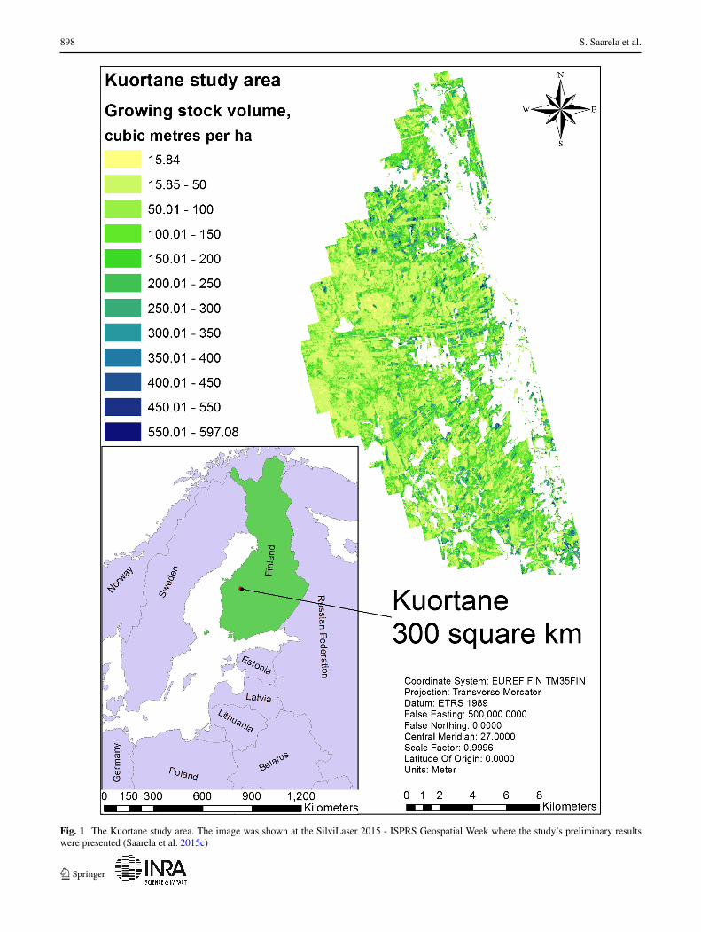
A copula population of 3×106 observations was created,based on which GSV was distributed over the study areausing nearest neighbour imputation with the Landsat andALS variables as a link, and a sample of 818,016 observa-tions corresponding to the 818,016 grid cells of 16m × 16msize, belonging to the land-use category forest. The selectedsample of 818,016 elements is our simulated populationwith simulated Landsat spectral values, ALS metrics andGSV values (Saarela et al. 2015b). An overview of the studypopulation is presented in Fig. 1:

3 Methods

3.1 Statistical approach

The model-based approach is based on the concept of asuperpopulation model. Any finite population of interestis seen as a sample drawn from a larger universe definedby the superpopulation model (Cassel et al. 1977). Forlarge populations, the model has fixed parameters, whosevalues are unknown, and random elements with assignedattributes. The model-based survey for a finite populationmean approximately corresponds to estimating the expectedvalue of the superpopulation mean (e.g., Stahl et al. 2016).Thus, in this study, our goal was to estimate the expectedvalue of the superpopulation mean, E(μ), for a large finitepopulation U with N grid cells as the population elements.Our first source of information is Landsat auxiliary data,which are available for each population element (grid cell).The second information source is a sample of M grid cells,denoted Sa . Each grid cell in Sa has two sets of RS auxil-iary data available: Landsat and ALS. The third source ofinformation is a subsample S of m grid cells, selected fromSa . For each element in S, Landsat, ALS, and GSV val-ues are available. For simplicity, simple random samplingwithout replacement was assumed to be performed in bothphases of sampling. The size of S was 10 % of Sa , and Sa

ranged from M = 500 to M = 10, 000 grid cells, i.e., S

ranged from m = 50 to m = 1000. We applied ordinaryleast square (OLS) estimators for estimating the regressionmodel parameters and their covariance matrices for mod-els that relate a response variable in one phase of samplingto the auxiliary data. One such example is ALS metricsregressed against GSV in the sample S. The OLS estimator

898 S. Saarela et al.

Fig. 1 The Kuortane study area. The image was shown at the SilviLaser 2015 - ISPRS Geospatial Week where the study’s preliminary resultswere presented (Saarela et al. 2015c)

Hierarchical model-based inference 899

was applied under the usual assumptions, i.e., (i) indepen-dence, assuming that the observations are identically andindependently distributed (i.i.d.); this assumption is guaran-teed by simple random sampling; (ii) exogeneity, assumingthat the (normally distributed) errors are uncorrelated withthe predictor variables, and (iii) identifiability, assumingthat there is one unique solution for the estimated modelparameters, i.e., (XT X) has full column rank.

Our study focused on the following cases:

Case A: Model-based estimation, where Landsat data areavailable wall-to-wall and GSV values are available forthe population elements in the sample S. In the followingsections, the case is also referred to as standard model-based inference.

Case B: Two-phase model-based estimation, where ALSdata are available for Sa and GSV values for the subsam-ple S. This case is also referred to as hybrid inference(Stahl et al. 2016), since it utilizes both model-basedinference and design-based inference.

Case C: Model-based estimation based on hierarchicalmodeling, with wall-to-wall Landsat data as the firstsource of information, ALS data from the sample Sa asthe second information source, and GSV data from thesubsample S as the third source of information. The caseis referred to as model-based inference with hierarchicalmodeling.

Case C was separated into three sub-cases. The differ-ence between the first two concerns the manner in whichthe three sources of data were utilized in the estimatorsand the corresponding variance and variance estimators.The third sub-case was introduced since it reflects howthis type of nested regression models have been used inprevious studies by simply ignoring the model step fromGSV to GSV predictions based on ALS data, i.e., bytreating the GSV predictions as if they were true values(e.g., Nelson et al. 2009; Neigh et al. 2011, 2013).

C.1: Predicting ALS predictor variables from Land-sat data – two-stage least squares regression. − Inthis case information from the subsample S was usedto estimate regression model parameters linking GSVvalues as responses with ALS variables as predic-tors. Information from Sa was then used to estimatea system of regression models linking ALS predic-tor metrics as response variables to Landsat variablesas predictors. Based on Landsat data ALS predictorvariables were then predicted for each population ele-ment and utilized for predicting GSV values with thefirst model. The reason for this rather complicatedapproach was that variances and variance estimatorscould be straightforwardly derived based on two-stageleast squares regression theory (e.g., Davidson andMacKinnon 1993).

C.2: Predicting GSV values from ALS data – hierar-chical model-based estimation. − In this case a modelbased on ALS data was used to predict GSV valuesfor all elements in Sa . The predicted GSV values werethen used for estimating a regression model linkingthe predicted GSV as a response variable with Landsatvariables as predictors. This model was then applied toall population elements in order to estimate the GSVpopulation mean.

C.3: Ignoring the uncertainty due to predicting GSVbased on ALS data—simplified hierarchical model-based estimation. In this case, the estimation proce-dure was the same as in C.2, but in the variance esti-mation we ignored the uncertainty due to predictingGSV values from ALS data. As mentioned previously,the reason for including this case is that this procedurehas been applied in several studies.

3.1.1 Case A: Standard model-based inference

This case follows well-established theory for model-basedinference (e.g., Matern et al. 1960; McRoberts 2006;Chambers & Clark 2012). For estimating the expected valueof the superpopulation mean E(μ) (Stahl et al. 2016), weutilise a regression model linking GSV values as responseswith Landsat variables as predictors using information fromthe subsample S. We assume a linear model to be appropri-ate, i.e.,

yS = ZSα + wS (1)

where yS is a column vector of length m of GSV values,ZS is a m × (q + 1) matrix of Landsat predictors (with afirst column of unit values and q is the number of Land-sat predictors), α is a column vector of model parameterswith length (q + 1), and wS is a column vector of randomerrors with zero expectation, of length m. Under assump-tions of independence, exogeneity, and identifiability (e.g.,Davidson and MacKinnon 1993), the OLS estimator of themodel parameters is

αS = (ZTS ZS)−1ZT

S yS (2)

where αS is a (q + 1)-length column vector of estimatedmodel parameters.

The estimated model parameters αS are then used forestimating the expected value of the population mean, E(μ),Stahl et al. (2016):

E(μ)A = ιTUZU αS (3)

900 S. Saarela et al.

where ιU is a N-length column vector, where each elementequals 1/N , ZU is a N ×(q+1) matrix of Landsat auxiliaryvariables, i.e., for the entire population.

The variance of the estimator E(μ)A is (Stahl et al.2016):

V[

E(μ)A

]

= ιTUZUCov(αS)ZTU ιU (4)

where Cov(αS) is the covariance matrix of the modelparameters αS . To obtain a variance estimator, the covari-ance matrix in Eq. 4 is replaced by an estimated covariancematrix.

When the errors, wS , in Eq. 1, are homoskedastic, theOLS estimator for the covariance matrix is (e.g., Davidsonand MacKinnon 1993):

CovOLS(αS) = wTS wS

m − q − 1(ZT

S ZS)−1 (5)

where wS = yS − ZS αS is a m-length column vectorof residuals over the sample S, using Landsat auxiliaryinformation.

When the errors, wS , in Eq. 1 are heteroskedastic, thecovariance matrix can be estimated consistently (HC) withthe estimator proposed by White (1980), namely

CovHC(αS) = (ZTS ZS)−1

[m

∑

i=1

w2i z

Ti zi

]

(ZTS ZS)−1 (6)

where wi is a residual and zi is a (q + 1)-length row vectorof Landsat predictors for the ith observation from the sub-sample S. To overcome an issue of the squared residuals w2

i

being biased estimators of the squared errors w2i , we applied

the correction mm−q−1 w2

i (Davidson and MacKinnon 1993),

i.e., all the w2i -terms in Eq. 6 were multiplied with m

m−q−1 .

3.1.2 Case B: Hybrid inference

In the case of hybrid inference, expected values and vari-ances were estimated by considering both the samplingdesign by which auxiliary data were collected and the modelused for predicting values of population elements based onthe auxiliary data (e.g., Stahl et al. 2016). For this case, alinear model linking ALS predictor variables and the GSVresponse variable were fitted using information from thesubsample S

yS = XSβ + eS (7)

where XS is the m × (p + 1) matrix of ALS predictors oversample S, β is a (p + 1)-length column vector of modelparameters, and eS is an m-length column vector of random

errors with zero expectation. Under assumptions of inde-pendence, exogeneity and identifiability the OLS estimatorof the model parameters is (e.g., Davidson & MacKinnon1993):

βS = (XTS XS)−1XT

S yS (8)

where βS is a (p + 1)-length column vector of estimatedmodel parameters.

Assuming simple random sampling without replacementin the first phase, a general estimator of the expected valueof the superpopulation mean E(μ) is (e.g., Stahl et al.2014):

E(μ)B = ιTSaXSa

βS (9)

where ιSa is a M-length column vector of entities 1/M andXSa is a M × (p + 1) matrix of ALS predictor variables.

The variance of the estimator E(μ)B is presented byStahl et al. (2014, Eq.5, p.5.), ignoring the finite populationcorrection factor:

V[

E(μ)B

]

= 1

Mω2 + ιTSa

XSaCov(βS)XTSa

ιSa (10)

where ω2 is the sample-based population variance from theM-length column vector of ySa

-values and Cov(βS) is thecovariance matrix of estimated model parameters βS . TheySa

values were estimated as

ySa= XSa

βS (11)

By replacing ω2 and Cov(βS) with the correspondingestimator, we obtain the variance estimator. The sample-based population variance ω2 is estimated by ω2 =

1M−1

∑Mi=1(yi − ¯y)2 (cf. Gregoire 2008), and the OLS

estimator for Cov(βS) is (e.g., Davidson & MacKinnon1993):

CovOLS(βS) = σ 2e (XT

S XS)−1 (12)

where σ 2e = eT

S eS

m−p−1 is the estimated residual variance and

eS = yS − XSβS is an m-length column vector of residuals

over sample S, using ALS auxiliary information.In the case of heteroscedasticity, the OLS estimator

(Eq. 8) can still be used for estimating the model parame-ters βS but the covariance matrix is estimated by the HCestimator (White 1980)

CovHC(βS) = (XTS XS)−1

[m

∑

i=1

e2i x

Ti xi

]

(XTS XS)−1 (13)

Hierarchical model-based inference 901

where ei is a residual and xi is the (p + 1)-length rowvector of ALS predictors for the ith observation from thesubsample S. Like for the Case A, we corrected the thesquared residuals e2

i by a factor mm−p−1 (Davidson and

MacKinnon 1993).

3.1.3 Case C: model-based inference with hierarchicalmodelling

We begin with introducing the hierarchical model-basedestimator for the expected value of the superpopulationmean, E(μ):

E(μ)C = ιTUZU(ZTSa

ZSa )−1ZT

SaXSa (X

TS XS)−1XT

S yS

(14)

where in addition to the already introduced notation, ZSa isa M × (q + 1) matrix of Landsat predictors for the sampleSa . In the following, it is shown that the hierarchical model-based estimators for Case C.1 and Case C.2 turn out tobe identical under OLS regression assumptions. In the caseof weighted least squares (WLS) regression, the estimatorsdiffer (see Appendix B).

C.1: Predicting ALS predictor variables from Landsatdata – two-stage least squares regression.

In this case, we applied a two-stage modeling approach(e.g., Davidson & MacKinnon 1993). Using the sampleSa , we developed a multivariate regression model link-ing ALS variables as responses and Landsat variables aspredictors, i.e.

xSaj= ZSaγ j + dj , [j=1, 2, ..., (p + 1)] (15)

where xSajis a M-length column vector of ALS variable

j , γ j is an (q+1)-length column vector of model param-eters for predicted ALS variable j , and dj is an M-lengthcolumn vector of random errors with zero expectation.We assumed that “all” Landsat predictors Z are used soZSa is the same for all variables xSaj

.There are (p+1)×(q+1) parameters γij in �, an (q+

1)× (p+1) matrix of model parameters, to be estimated.If we assume simultaneous normality the simultaneousleast squares estimator can be used as:

γ j = (ZTSa

ZSa )−1ZT

SaxSaj

(16)

We denote � as a (q + 1) × (p + 1) matrix of esti-mated model parameters, where the first column of �

is the column vector (ZTSa

ZSa )−1ZT

Sa1M , which equals

(

1 0 · · · 0)T

1×(q+1), where 1M is an M-length column

vector of unit values. Thus, we can predict ALS variablesfor all population elements using Landsat variables, i.e.:

XU = ZU� (17)

where XU is a N × (p + 1) matrix of predicted ALSvariables over the entire population U .

Then, the predicted ALS variables XU were coupledwith the estimated model parameters βS from Eq. 8 toestimate the expected value of the mean GSV:

E(μ)C.1 = ιTUXU

βS (18)

To show that this equals Eq. 14, we can rewrite Eq. 18,using Eq. 8, as

E(μ)C.1 = ιTUXU(XT

S XS)−1XTS yS

which evidently is equivalent to

E(μ)C.1 = ιTUZU�(XT

S XS)−1XTS yS (19)

Finally, using the estimator for � (Eq. 16), we canrewrite Eq. 19 as

E(μ)C.1 = ιTUZU(ZTSa

ZSa )−1ZT

SaXSa (X

TS XS)−1XT

S yS

which coincides with Eq. 14 proposed at the start of thissection.

Since Eq. 18 can be rewritten as E(μ)C.1 =∑p+1

i=1 ιTU xUiβSi

, the variance V[

E(μ)C.1

]

of the estima-

tor in Eq. 18 can be expressed as

V[

E(μ)C.1

]

=p+1∑

i=1

p+1∑

j=1

Cov(βSi[ιTU xUi

], βSj[ιTU xUj

])

(20)

Since βS is based on the subsample S and XU isbased on the sample Sa , eS and dj are considered to beindependent, and as a consequence we have

Cov(βSi[ιTU xUi

], βSj[ιTU xUj

]) = βiβjCov([ιTU xUi], [ιTU xUj

])+[ιTUxUi

][ιTUxUj]Cov(βSi

, βSj)

+Cov(βSi, βSj

)Cov([ιTU xUi], [ιTU xUj

]) (21)

The covariances Cov(βSi, βSj

) are given by the ele-ments of the matrix σ 2

e (XTS XS)−1, where σ 2

e is the vari-

ance of the residuals eS , estimated as σ 2e = eT

S eS

m−p−1 (same

as in Section 3.1.2). Thus, we estimate Cov(βSi, βSj

) as

Cov(βSi, βSj

) = σ 2e (XT

S XS)−1ij (22)

902 S. Saarela et al.

Further, Eq. 17 gives

Cov([ιTU xUi], [ιTU xUj

]) =q+1∑

k=1

q+1∑

l=1

[ιTUzUk][ιTUzUl

]Cov(γki , γlj )

(23)

The covariance of the estimated model parameters �,assuming homoskedasticity,

Cov(γki , γlj ) = Cov(�) = �(ZTSa

ZSa )−1 (24)

where � is a (p + 1) × (p + 1) matrix of covariancesof the M × (p + 1) matrix of residuals D, which areestimated as D = XSa − ZSa

�, hence the covariancematrix � is estimated as:

� =D

TD

M − q − 1(25)

Combining Eqs. 20–24, we can derive the least squares

(LS) variance V[

E(μ)C.1

]

:

VLS

[

E(μ)C.1

]

= 1

N2

N∑

i=1

N∑

j=1

(

zi (ZTSa

ZSa )−1zT

j βT �β

+σ 2e zi

�(XTS XS)−1

�TzTj

+σ 2e zi (Z

TSa

ZSa )−1zT

j

p+1∑

k=1

p+1∑

l=1

λkl(XTS XS)−1

kl

)

= ιTUZU (ZTSa

ZSa )−1ZT

U ιU βT �β

+ιTU ZU�CovOLS(βS)�

TZT

U ιU

+σ 2e ιTU ZU (ZT

SaZSa )

−1ZTU ιU

p+1∑

k=1

p+1∑

l=1

λkl(XTS XS)−1

kl

(26)

Here, λkl is the [k, l]th element of he matrix �.

To derive an estimator VLS

[

E(μ)C.1

]

for the variance

Eq. 26, we replace β with estimated βS , the covariancematrix � with � from Eq. 25, and σ 2

e with the estimatedσ 2

e . Knowing that E(βSiβSj

) = βiβj + Cov(βSiβSj

)

we have a “minus” sign between the second and thirdterms of Eq. 26 due to subtracting a product of the esti-mated covariances. Hence, our estimator for the varianceVLS

[

E(μ)C.1

]

is

VLS

[

E(μ)C.1

]

= ιTUZU (ZTSa

ZSa )−1ZT

U ιUβT

S�βS

+ιTU ZU� CovOLS(βS)�

TZT

U ιU

−σ 2e ιTU ZU (ZT

SaZSa )

−1ZTU ιU

p+1∑

k=1

p+1∑

l=1

λkl (XTS XS)−1

kl

(27)

where λkl is a [k, l]th element of the estimated covariancematrix � of residuals D.

In the special case when any potential heteroskedasti-ciy is limited to the GSV function of ALS predictor vari-ables over the sample S, the heteroskedasticity-consistentvariance estimator is:

VHC

[

E(μ)C.1

]

= ιTU ZU (ZTSa

ZSa )−1ZT

U ιUβT

S�βS

+ιTU ZU� CovHC(βS)�

TZT

U ιU

−ιTU ZU (ZTSa

ZSa )−1ZT

U ιU

p+1∑

k=1

p+1∑

l=1

λklCovHC(βS)kl

(28)

C.2: Predicting GSV values from ALS data – hierarchi-cal model-based estimation.

In this case, the predicted GSV variable ySais used as

a response variable for estimating model parameters link-ing GSV and Landsat-based predictors over the sampleSa , i.e., our assumed model is

XSaβ = ZSaα + wSa (29)

where XSaβ is an M-length column vector of expectedvalues of predicted GSV values ySa

= XSaβS using ALS

data, α is a (q+1)-length column vector of model param-eters linking estimated GSV values and Landsat predictorvariables, and wSa is an M-length column vector ofrandom errors with zero expectation.

In case the XSaβ values were observable, the OLSestimator of α would be

αSa = (ZTSa

ZSa )−1ZT

SaXSaβ (30)

However, we use the XSaβS values and thus our OLS

estimator of α is

αSa = (ZTSa

ZSa )−1ZT

SaXSa

βS (31)

Thus, using the estimator βS (Eq. 8), we obtain:

αSa = (ZTSa

ZSa )−1ZT

SaXSa (X

TS XS)−1XT

S yS (32)

Then the estimated model parameters αSa wereemployed for estimating the expected value of superpop-ulation mean E(μ):

E(μ)C.2 = ιTUZU αSa

= ιTUZU(ZTSa

ZSa )−1ZT

SaXSa (X

TS XS)−1XT

S yS

which coincides with Eq. 14. Thus, for models withhomogeneous random errors, the estimators of theexpected mean are the same for Cases C.1 and C.2.

Hierarchical model-based inference 903

Based on the estimator E(μ)C.2 = ιTUZU αSa , thevariance is Stahl et al. (2016)

V[

E(μ)C.2

]

= ιTUZUCov(αSa )ZTU ιU (33)

where Cov(αSa ) is the covariance matrix of αSa .By replacing the covariance Cov(αSa ) with estimatedcovariance Cov(αSa ) in the expression Eq. 33, we obtaina variance estimator.

Under OLS assumptions Cov(αSa ) is estimated as

CovOLS (αSa ) = wTSa

wSa

M − q − 1(ZT

SaZSa )

−1

+(ZTSa

ZSa )−1ZT

Sa

[

XSaCovOLS(βS)XT

Sa

]

ZSa (ZTSa

ZSa )−1

(34)

where, wSa = XSaβS −ZSa αSa is an M-length vector of

residuals.For the derivation of the estimator in Eq. 34, see

Appendix C.In case of heteroskedasticy of the random errors in the

sample Sa and the sample S, the HC covariance matrixestimator (White 1980) of the estimated model parame-ters αSa was applied (like before, the OLS estimator forαSa was used):

CovHC (αSa ) = (ZTSa

ZSa )−1

[M

∑

i=1

w2i z

Ti zi

]

(ZTSa

ZSa )−1

+(ZTSa

ZSa )−1ZT

Sa

[

XSaCovHC(βS)XT

Sa

]

ZSa (ZTSa

ZSa )−1

(35)

where w2i is a squared residual for the ith observation

in the sample Sa . As in Cases A and B, we applied thecorrection M

M−q−1 w2i (Davidson and MacKinnon 1993).

A derivation of the estimator (Eq. 35) is given in seeAppendix C.

C.3: Ignoring the uncertainty due to predicting GSVvalues based on ALS data – simplified hierarchicalmodel-based estimation.

This case is included since several studies have usedpredicted values ySa

, using ALS models, as if they weretrue values, and hence, the uncertainty of their estimationhas been ignored. In this case, the same estimator (Eq. 14)for the expected value of mean was used, but for the vari-ance estimator, Eqs. 33 and 34 were applied. Under OLSassumption, the matrix Cov(αSa ) was estimated as

CovOLS(αSa )C.3 = wTSa

wSa

M − q − 1(ZT

SaZSa )

−1 + 0 (36)

In the case of heteroskedasticity, it was estimated as

CovHC(αSa )C.3 =(ZTSa

ZSa )−1

[M

∑

i=1

w2i z

Ti zi

]

(ZTSa

ZSa )−1+0

(37)

Thus, in these estimators, we ignored the uncertaintydue to the regression model based on information fromthe sample S.

3.2 Sampling simulation

Monte Carlo sampling simulation with R = 3 × 104 repeti-tions was applied. At each repetition, new regression modelparameter estimates for the pre-selected variables and theircorresponding covariance matrix estimates were computed.Based on the computed model parameters, the expectedvalue of the population mean and its variance were esti-mated for each case. Averages of estimated values E(μ) and

their estimated variances V[

E(μ)]

were recorded. Empir-

ical variances V[

E(μ)]

empwere computed based on the

outcomes from the R repetitions as

V[

E(μ)]

emp= 1

R − 1

R∑

k=1

[

E(μ)k − E(μ)

]2

(38)

Further, the empirical mean square error (MSE) wasestimated based on the R repetitions

MSE[

E(μ)]

emp= 1

R

R∑

k=1

[

E(μ)k − E(μ)]2

(39)

with the known expected value of the superpopulation meanE(μ) = 104.27 m3ha−1, as the simulated finite populationmean.

For all cases, we calculated the relative bias of theestimated variance

RelBIAS = 100% ×V

[

E(μ)]

− V[

E(μ)]

emp

V[

E(μ)]

emp

(40)

In order to make sure that the number of repetitions inthe Monte Carlo simulations was sufficient, we graphedthe average value of the target parameter estimates versusthe number of simulation repetitions. For all our cases and

904 S. Saarela et al.

Fig. 2 The convergence of the estimated model-based variance under OLS assumptions V OLS

[

E(μ)]

over the number of repetitions in the

Monte Carlo simulations, sample sizes: m = 100 grid cells, M = 1000 grid cells.

estimators, the graphs showed that the estimators stabilizedfairly rapidly and that our 3×104 repetitions were sufficient.An example is shown in Fig. 2, for the case of estimatingV OLS

[

E(μ)]

:

4 Results

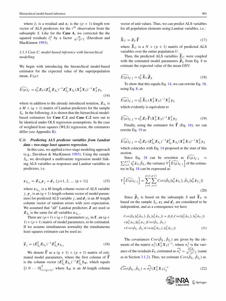
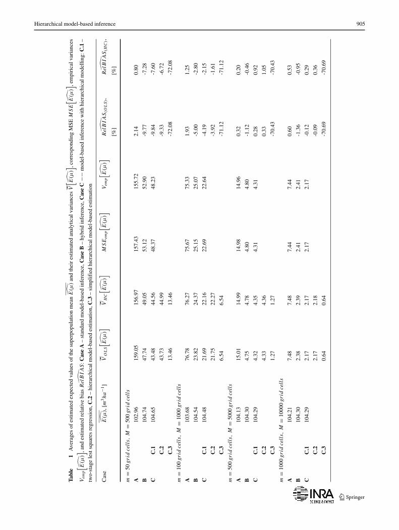
As expected, the accuracy of the model-based estimatorwith hierarchical modeling (Case C) increased as samplesizes in the two phases increased. The estimator is at leastapproximately unbiased, because for every group of sam-

ple sizes MSEemp

[

E(μ)]

≈ Vemp

[

E(μ)]

. The Landsat

variables had less predictive power than ALS metrics in pre-diction GSV; hence, the accuracy of the Case B estimatoris higher than the Case A estimator. However, includingwall-to-wall Landsat auxiliary information improved theaccuracy compared to using ALS sample data alone, i.e., theMSE of Case C is lower than the MSE of Case B (Table 1).

Comparing the performances of the Case C.3 varianceestimator and the hierarchical model-based variance estima-tor of Case C.2, we observed that ignoring the uncertaintydue to the GSV-ALS model leads to underestimation of thevariance by about 70 % (Table 1).

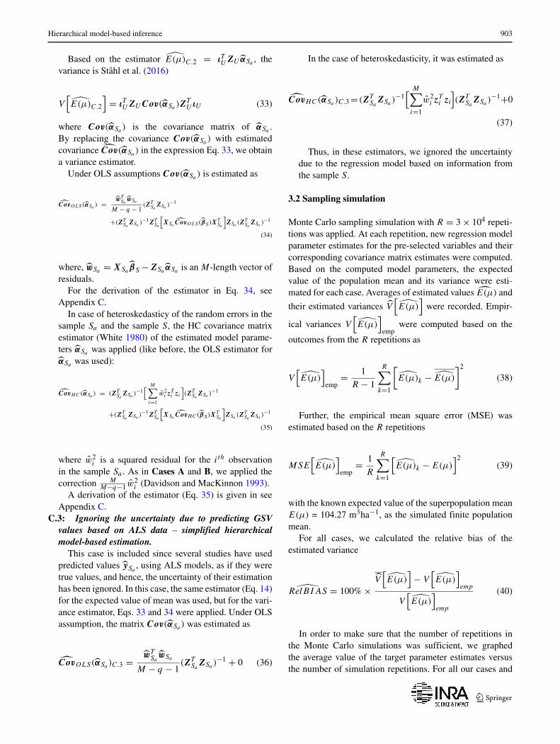
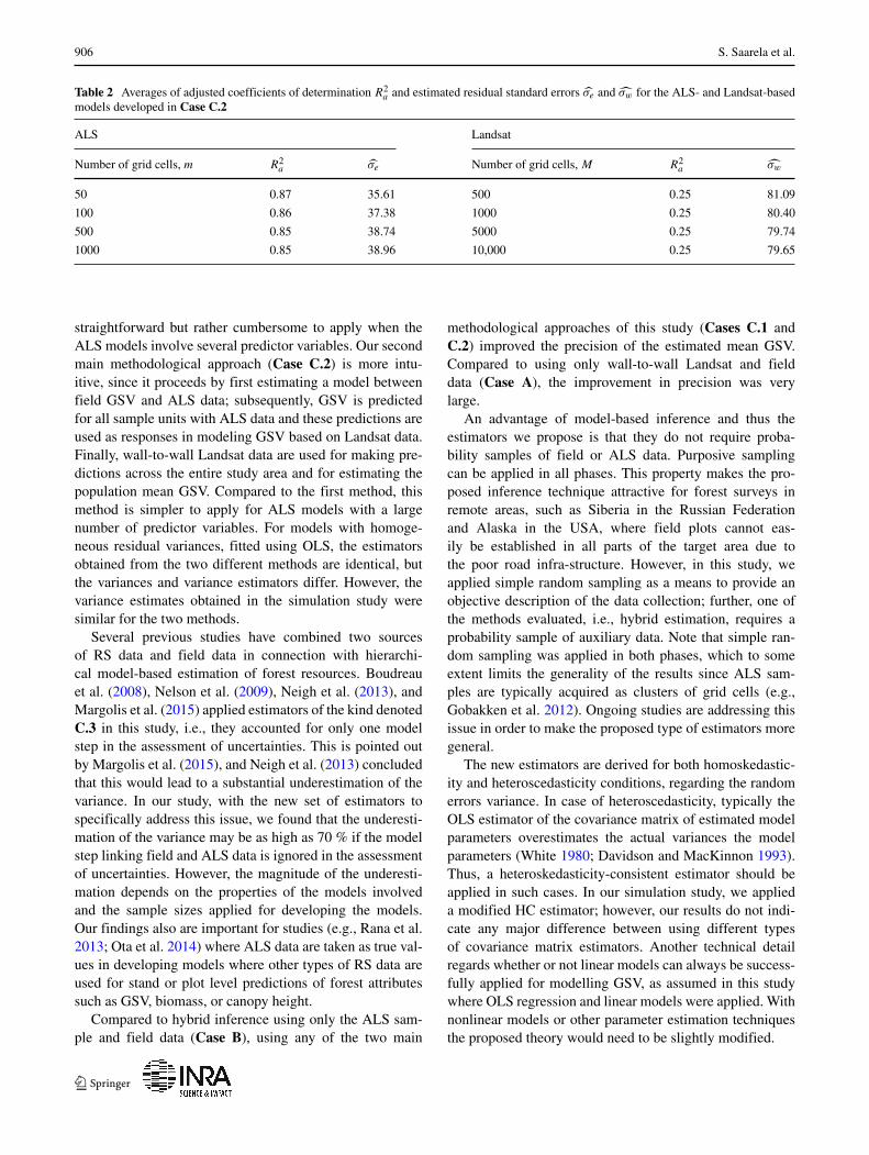
In Table 2, we present examples of the goodness of fit ofthe models used in the Case C.2 (and C.3). From Table 2,

it can be observed that the goodness of fit was substantiallybetter for the ALS models compared to the Landsat models.

5 Discussion

In this study, we have presented and evaluated novel esti-mators and their corresponding variance estimators formodel-based inference using three sources of informationand hierarchically nested models, for applications in for-est inventory combining RS and field data. The estimatorswere evaluated through Monte Carlo simulation, for thecase of estimating the population mean GSV. The esti-mators and the variance estimators were found to be atleast approximately unbiased, unless in the Case C.3 wherethe uncertainty of one of the models was ignored. Theprecision of the estimators depended on the number ofobservations used for developing the models involved; theuncertainties due to both model steps involved were foundto substantially contribute to the overall uncertainty of theestimators.

Our first main methodological approach (Case C.1) useswall-to-wall Landsat data to predict the ALS predictor vari-ables involved when regressing field-measured GSV as aresponse variable on ALS data. In this way, we emulatedwall-to-wall ALS data, which were used for estimatingthe population mean across the study area. The method is

Hierarchical model-based inference 905

Tabl

e1

Ave

rage

sof

estim

ated

expe

cted

valu

esof

the

supe

rpop

ulat

ion

mea

n E(μ

)an

dth

eir

estim

ated

anal

ytic

alva

rian

ces

V[

E(μ

)]

,cor

resp

ondi

ngM

SEM

SE

[

E(μ

)]

,em

piri

calv

aria

nces

Vem

p

[

E(μ

)]

,and

estim

ated

rela

tive

bias

R

elB

IA

S:C

ase

A–

stan

dard

mod

el-b

ased

infe

renc

e,C

ase

B–

hybr

idin

fere

nce,

Cas

eC

−−m

odel

-bas

edin

fere

nce

with

hier

arch

ical

mod

ellin

g:C

.1–

two-

stag

ele

stsq

uare

sre

gres

sion

,C.2

–hi

erar

chic

alm

odel

-bas

edes

timat

ion,

C.3

–si

mpl

ifie

dhi

erar

chic

alm

odel

-bas

edes

timat

ion

Cas

e E(μ

),[m

3ha

−1]

VO

LS

[

E(μ

)]

VH

C

[

E(μ

)]

MSE

em

p

[

E(μ

)]

Vem

p

[

E(μ

)]

R

elB

IA

S(O

LS),

R

elB

IA

S(H

C),

[%]

[%]

m=

50grid

cells,

M=

500

grid

cells

A10

2.96

159.

0515

6.97

157.

4315

5.72

2.14

0.80

B10

4.74

47.7

449

.05

53.1

252

.90

-9.7

7-7

.28

CC

.110

4.65

43.4

844

.56

48.3

748

.23

-9.8

4-7

.60

C.2

43.7

344

.99

-9.3

3-6

.72

C.3

13.4

613

.46

-72.

08-7

2.08

m=

100

grid

cells,

M=

1000

grid

cells

A10

3.68

76.7

876

.27

75.6

775

.33

1.93

1.25

B10

4.54

23.8

224

.37

25.1

525

.07

-5.0

0-2

.80

CC

.110

4.48

21.6

922

.16

22.6

922

.64

-4.1

9-2

.15

C.2

21.7

522

.27

-3.9

2-1

.61

C.3

6.54

6.54

-71.

12-7

1.12

m=

500

grid

cells,

M=

5000

grid

cells

A10

4.13

15.0

114

.99

14.9

814

.96

0.32

0.20

B10

4.30

4.75

4.78

4.80

4.80

-1.1

2-0

.46

CC

.110

4.29

4.32

4.35

4.31

4.31

0.28

0.92

C.2

4.33

4.36

0.33

1.05

C.3

1.27

1.27

-70.

43-7

0.43

m=

1000

grid

cells,

M=

1000

0grid

cells

A10

4.21

7.48

7.48

7.44

7.44

0.60

0.53

B10

4.30

2.38

2.39

2.41

2.41

-1.3

6-0

.95

CC

.110

4.29

2.17

2.17

2.17

2.17

-0.1

20.

29

C.2

2.17

2.18

-0.0

90.

36

C.3

0.64

0.64

-70.

69-7

0.69

906 S. Saarela et al.

Table 2 Averages of adjusted coefficients of determination R2a and estimated residual standard errors σe and σw for the ALS- and Landsat-based

models developed in Case C.2

ALS Landsat

Number of grid cells, m R2a σe Number of grid cells, M R2

a σw

50 0.87 35.61 500 0.25 81.09

100 0.86 37.38 1000 0.25 80.40

500 0.85 38.74 5000 0.25 79.74

1000 0.85 38.96 10,000 0.25 79.65

straightforward but rather cumbersome to apply when theALS models involve several predictor variables. Our secondmain methodological approach (Case C.2) is more intu-itive, since it proceeds by first estimating a model betweenfield GSV and ALS data; subsequently, GSV is predictedfor all sample units with ALS data and these predictions areused as responses in modeling GSV based on Landsat data.Finally, wall-to-wall Landsat data are used for making pre-dictions across the entire study area and for estimating thepopulation mean GSV. Compared to the first method, thismethod is simpler to apply for ALS models with a largenumber of predictor variables. For models with homoge-neous residual variances, fitted using OLS, the estimatorsobtained from the two different methods are identical, butthe variances and variance estimators differ. However, thevariance estimates obtained in the simulation study weresimilar for the two methods.

Several previous studies have combined two sourcesof RS data and field data in connection with hierarchi-cal model-based estimation of forest resources. Boudreauet al. (2008), Nelson et al. (2009), Neigh et al. (2013), andMargolis et al. (2015) applied estimators of the kind denotedC.3 in this study, i.e., they accounted for only one modelstep in the assessment of uncertainties. This is pointed outby Margolis et al. (2015), and Neigh et al. (2013) concludedthat this would lead to a substantial underestimation of thevariance. In our study, with the new set of estimators tospecifically address this issue, we found that the underesti-mation of the variance may be as high as 70 % if the modelstep linking field and ALS data is ignored in the assessmentof uncertainties. However, the magnitude of the underesti-mation depends on the properties of the models involvedand the sample sizes applied for developing the models.Our findings also are important for studies (e.g., Rana et al.2013; Ota et al. 2014) where ALS data are taken as true val-ues in developing models where other types of RS data areused for stand or plot level predictions of forest attributessuch as GSV, biomass, or canopy height.

Compared to hybrid inference using only the ALS sam-ple and field data (Case B), using any of the two main

methodological approaches of this study (Cases C.1 andC.2) improved the precision of the estimated mean GSV.Compared to using only wall-to-wall Landsat and fielddata (Case A), the improvement in precision was verylarge.

An advantage of model-based inference and thus theestimators we propose is that they do not require proba-bility samples of field or ALS data. Purposive samplingcan be applied in all phases. This property makes the pro-posed inference technique attractive for forest surveys inremote areas, such as Siberia in the Russian Federationand Alaska in the USA, where field plots cannot eas-ily be established in all parts of the target area due tothe poor road infra-structure. However, in this study, weapplied simple random sampling as a means to provide anobjective description of the data collection; further, one ofthe methods evaluated, i.e., hybrid estimation, requires aprobability sample of auxiliary data. Note that simple ran-dom sampling was applied in both phases, which to someextent limits the generality of the results since ALS sam-ples are typically acquired as clusters of grid cells (e.g.,Gobakken et al. 2012). Ongoing studies are addressing thisissue in order to make the proposed type of estimators moregeneral.

The new estimators are derived for both homoskedastic-ity and heteroscedasticity conditions, regarding the randomerrors variance. In case of heteroscedasticity, typically theOLS estimator of the covariance matrix of estimated modelparameters overestimates the actual variances the modelparameters (White 1980; Davidson and MacKinnon 1993).Thus, a heteroskedasticity-consistent estimator should beapplied in such cases. In our simulation study, we applieda modified HC estimator; however, our results do not indi-cate any major difference between using different typesof covariance matrix estimators. Another technical detailregards whether or not linear models can always be success-fully applied for modelling GSV, as assumed in this studywhere OLS regression and linear models were applied. Withnonlinear models or other parameter estimation techniquesthe proposed theory would need to be slightly modified.

Hierarchical model-based inference 907

Although some simplifying assumptions were made, wesuggest that the proposed set of estimators (Cases C.1and C.2) has a potential to substantially contribute to thedevelopment of new techniques for large-area forest sur-veys, utilizing several sources of auxiliary information inconnection with model-based inference.

Open Access This article is distributed under the terms of theCreative Commons Attribution 4.0 International License (http://creativecommons.org/licenses/by/4.0/), which permits unrestricteduse, distribution, and reproduction in any medium, provided you giveappropriate credit to the original author(s) and the source, provide alink to the Creative Commons license, and indicate if changes weremade.

Appendix A: Reference data

A.1 Study site

To demonstrate the validity of our estimators, we chose theKuortane area in the southern Ostrobothnia region of west-ern Finland as study site. The main reason for this was theavailability of data from earlier studies that have been con-ducted in the same region (e.g., Saarela et al. 2015b, 2016).The area has a size of approximately 30,000 ha of which20,941 ha are covered by forests with Pinus sylvestris beingthe main tree species. Picea abies and Betula spp. usuallyoccur as mixtures. The remaining parts of the landscape areformed by peat lands and open mires on higher elevations,and agricultural fields and water bodies at lower elevationsand terrain depressions, respectively.

A.2 Field data

Field data were collected in 2006 using a systematic sampleof circular field plots that were arranged in clusters. Eachcluster consisted of 18 plots with a radius of 9 m, and thesample covered all land use types. For this study, however,only plots in forest areas were considered for further analy-sis. The distance between plots in a cluster was 200 m andthe distance between clusters was 3500 m. In total, mea-surements from 441 forest field plots were available. GSVvalues per hectare were calculated for each field plot follow-ing the Finnish National Forest Inventory (NFI) procedure(Tomppo et al. 2008). Plots with GSV values of zero wereomitted.

At all trees with a diameter at breast height (dbh) largerthan 5 cm the following variables were observed: dbh, treestory class, and tree species. Tree height was measured forone sample tree per plot and species, while height for theremaining trees was predicted using models from Veltheim(1987). For calculating GSV, which is our variable of inter-est, individual tree models from Laasasenaho (1982) were

applied. Individual tree volumes were then aggregated onthe plot level and expanded to per hectare values.

A.3 ALS data

ALS of the study area was conducted in July 2006 usingan Optech 3100 laser scanning system. The average fly-ing altitude above terrain was 2000 m. The mean footprintdiameter was 60 cm and the average point density was 0.64echoes m−2. Altogether, 19 north-south oriented flight lineswere flown using a side overlap of about 20 %. The pointcloud was normalized to terrain height using a digital ter-rain model generated with the Orientation and Processingof Airborne Laser Scanning data (OPALS) software (Pfeiferet al. 2014) from the same data, and divided along a grid of16x16 m large cells. For each cell and field plot the heightvalues of laser echoes were used to calculate several metricsrelated to observed values of GSV. Four metrics were cal-culated with the FUSION software (McGaughey 2012), andused for this study: maximum height observation (hmax); the80th percentile of the distribution of height values (h80); thecanopy relief ratio (CRR); and the number of returns above2 m divided by the total number of returns as a measure forcanopy cover (pveg). For details about the ALS data, seeSaarela et al. (2015a).

A.4 Landsat data

Landsat 7 ETM+ orthorectified (L1T) multi-spectralimagery data were downloaded from U.S. Geological Sur-vey (2014). The images were acquired in June 2006. Foreach field plot and grid cell, digital numbers of spectralvalues from the green (B20), red (B30), and shortwave infra-red (B50) bands were extracted using the nearest neighbourre-sampling method in ArcGIS software (ESRI 2011).

Appendix B: Weighted least squares regressionestimator for the model-based inference in CaseC.1

In the case of applying weighted least squares estimatorfor heteroskedasticity removal in Case C.1, the estimator(Eq.(8)) will have the following form

βS = (XTS G−1

S XS)−1XTS G−1

S yS (41)

where GS is a m × m diagonal matrix with weight elementsin the diagonal and zeros outside of the diagonal.

The estimator [corresponding to Eq. 16] will be

γ j = (ZTSa

H−1Saj

ZSa )−1ZT

SaH−1

SajxSaj

(42)

where H Sajis a M × M diagonal matrix with weight ele-

ments in the diagonal and zeros outside of the diagonal for

908 S. Saarela et al.

j th ALS variable over sample Sa , and xSajis an M-length

column vector of j th ALS variable.Thus, estimator for the expected value of the superpopu-

lation mean estimation in Case C.1 will be

E[μC.1]WLS =

ιTUZU

⎛

⎜

⎜

⎜

⎜

⎜

⎜

⎜

⎜

⎝

(

γ (p+1) = (ZTSa

H−1Sa (p+1)

ZSa )−1ZT

SaH−1

Sa (p+1)xSa (p+1)

)T

(

γ p = (ZTSa

H−1Sap

ZSa )−1ZT

SaH−1

SapxSap

)T

.

.

.(

γ 2 = (ZTSa

H−1Sa2

ZSa )−1ZT

SaH−1

Sa2xSa2

)T

(

γ 1 = (ZTSa

H−1Sa1

ZSa )−1ZT

SaH−1

Sa11M

)T

⎞

⎟

⎟

⎟

⎟

⎟

⎟

⎟

⎟

⎠

T

×(XTS G−1

S XS)−1XTS G−1

S yS (43)

Appendix C Proof of the hierarchical model-basedvariance estimators in Case C.2.

C.1 General derivation

For each element in the sample Sa , there are two models:yi = xiβ + ei with e ∼ N(σ 2

e , 0) and xiβ = ziα +wi withw ∼ N(σ 2

w, 0), where yi is GSV value, xi is an (p + 1)-length row vector of ALS predictor variables, zi is a (q +1)-length row vector of Landsat predictor variables, and ei

and wi are independent and identically distributed (i.i.d.)random errors for the ith observation. Combining these twomodels, we can develop a composite model:

xiβ = ziα + wi

yi − ei = ziα + wi

yi = ziα + wi + ei (44)

That is, in vector notation the regression model appliedin Case C.2 is

ySa= ZSaα + wSa + eSa (45)

For deriving an estimator for the covariance matrix of theestimated model parameters αSa , we modify Eq. 32 as:

αSa = (ZTSa

ZSa )−1ZT

SaXSa (X

TS XS)−1XT

S yS

= (ZTSa

ZSa )−1ZT

SaXSa (X

TS XS)−1XT

S (XSβ + eS)

= (ZTSa

ZSa )−1ZT

SaXSa (X

TS XS)−1XT

S XSβ

+(ZTSa

ZSa )−1ZT

SaXSa (X

TS XS)−1XT

S eS

Knowing that (XTS XS)−1XT

S XS = I (m×m) in the firstterm of the expression, we obtain:

αSa = (ZTSa

ZSa )−1ZT

SaXSaβ

+(ZTSa

ZSa )−1ZT

SaXSa (X

TS XS)−1XT

S eS

Recalling from Eq. 44 that XSaβ = ZSaα + wSa , wemodify further to obtain:

αSa = (ZTSa

ZSa )−1ZT

Sa(ZSaα + wSa )

+(ZTSa

ZSa )−1ZT

SaXSa (X

TS XS)−1XT

S eS

= (ZTSa

ZSa )−1ZT

SaZSaα + (ZT

SaZSa )

−1ZTSa

wSa

+(ZTSa

ZSa )−1ZT

SaXSa (X

TS XS)−1XT

S eS

Knowing that (ZTSa

ZSa )−1ZT

SaZSa = I (M×M), we

obtain:

αSa = α + (ZTSa

ZSa )−1ZT

SawSa

+(ZTSa

ZSa )−1ZT

SaXSa (X

TS XS)−1XT

S eS

Moving α to the left side of the expression, we get

αSa − α = (ZTSa

ZSa )−1ZT

SawSa

+(ZTSa

ZSa )−1ZT

SaXSa (X

TS XS)−1XT

S eS (46)

Now, we derive the estimator for the covariance of αSa :

Cov(αSa ) = E[

(αSa − α)(αSa − α)T]

= E[

(

(ZTSa

ZSa )−1ZT

SawSa + (ZT

SaZSa )

−1ZTSa

XSa (XTS XS)−1XT

S eS

)

×(

(ZTSa

ZSa )−1ZT

SawSa + (ZT

SaZSa )

−1ZTSa

XSa (XTS XS)−1XT

S eS

)T]

= E[

(ZTSa

ZSa )−1ZT

SawSa

(

(ZTSa

ZSa )−1ZT

SawSa

)T

+(ZTSa

ZSa )−1ZT

SawSa

(

(ZTSa

ZSa )−1ZT

SaXSa (X

TS XS)−1XT

S eS

)T

+(ZTSa

ZSa )−1ZT

SaXSa (X

TS XS)−1XT

S eS

(

(ZTSa

ZSa )−1ZT

SawSa

)T

+(ZTSa

ZSa )−1ZT

SaXSa (X

TS XS)−1XT

S eS

(

(ZTSa

ZSa )−1ZT

SaXSa (X

TS XS)−1XT

S eS

)T]

= (ZTSa

ZSa )−1ZT

SaE

[

wSawTSa

]

ZSa (ZTSa

ZSa )−1 + (ZT

SaZSa )

−1ZTSa

E[

wSaeTS

]

XS(XTS XS)−1XT

SaZSa (Z

TSa

ZSa )−1

+(ZTSa

ZSa )−1ZT

SaXSa (X

TS XS)−1XT

S E[

eSwTSa

]

ZSa (ZTSa

ZSa )−1

+(ZTSa

ZSa )−1ZT

SaXSa (X

TS XS)−1XT

S E[

eSeTS

]

XS(XTS XS)−1XT

SaZSa (Z

TSa

ZSa )−1

Hierarchical model-based inference 909

Assuming that wSa and eS are independent and uncor-related, and knowing that E[wSa ] = 0 and E[eSa ] = 0,

we have E[

wSaeTS

]

= E[

eSwTSa

]

= E[

wSa

]

E[

eS

]

= 0.

Thus,

Cov(αSa ) = (ZTSa

ZSa )−1ZT

SaE

[

wSawTSa

]

ZSa (ZTSa

ZSa )−1

+(ZTSa

ZSa )−1ZT

SaXSa (X

TS XS)−1XT

S E[

eSeTS

]

XS(XTS XS)−1XT

SaZSa (Z

TSa

ZSa )−1

= (ZTSa

ZSa )−1ZT

Sa�ZSa (Z

TSa

ZSa )−1

+(ZTSa

ZSa )−1ZT

SaXSa (X

TS XS)−1XT

S XS(XTS XS)−1XT

SaZSa (Z

TSa

ZSa )−1 (47)

where � is a covariance matrix of errors wSa and is acovariance matrix of errors eS .

C.2 Under homogeneous random errors

Under the general OLS assumptions � = σ 2wI (M×M),

where σ 2w is estimated as σ 2

w = wSa wTSa

M−q−1 , where wSa =XSa

βS − ZSa αSa is an M-length column vector of resid-uals over sample Sa . Thus, first part of Eq. 47, i.e.,

(ZTSa

ZSa )−1ZT

Sa�ZSa (Z

TSa

ZSa )−1, can be estimated as

(ZTSa

ZSa )−1ZT

Sa

[

σw2I (M×M)

]

ZSa (ZTSa

ZSa )−1

= wSa wTSa

M − q − 1(ZT

SaZSa )

−1

In the second term of Eq. 47, is estimated asσ 2

e I (m×m) = eS eTS

m−q−1I (m×m), where eS = yS − XSβS is

an m-length column vector of residuals over the sample S.Thus, the second term can be estimated as

(ZTSa

ZSa )−1ZT

SaXSa (X

TS XS)−1XT

S

[ eS eTS

m − q − 1I (m×m)

]

XS(XTS XS)−1XT

SaZSa (Z

TSa

ZSa )−1

= (ZTSa

ZSa )−1ZT

SaXSa

[ eS eTS

m − q − 1(XT

S XS)−1]XTSa

ZSa (ZTSa

ZSa )−1

We can see that the expression[ eS eT

S

m−q−1 (XTS XS)−1

]

is infact the estimator of the covariance matrix of the estimatedmodel parameters βS (Eq. 12). Therefore, we can write theestimator of Cov(αSa ) as

CovOLS (αSa ) = wSa wTSa

M − q − 1(ZT

SaZSa )

−1

+(ZTSa

ZSa )−1ZT

Sa

[

XSaCovOLS(βS)XT

Sa

]

ZSa (ZTSa

ZSa )−1

(48)

C.3 Under heteroskedasticity

In the case of heteroskedasticity, we followed the theo-retical framework developed by White (1980). Thus, theexpression ZT

Sa�ZSa in the first term of Eq. 47 can be esti-

mated as∑M

i=1 w2i z

Ti zi ; correspondingly, in the second term

the expression XTS XS can be estimated as

∑mi=1 e2

i xTi xi .

Further, the second term of Eq. 47 can be estimated as

(ZTSa

ZSa )−1ZT

SaXSa (X

TS XS)−1[

m∑

i=1

e2i x

Ti xi

]

(XTS XS)−1XT

SaZSa (Z

TSa

ZSa )−1

We can see that (XTS XS)−1

[ ∑mi=1 e2

i xTi xi

]

(XTS XS)−1

is in fact the heteroskedasticity-consistent estimator ofthe covariance matrix of the estimated model parametersβS (Eq. 13). Therefore, the heteroskedasticity-consistentcovariance matrix estimator for the estimated model param-eters αSa is

CovHC(αSa ) = (ZTSa

ZSa )−1

[M

∑

i=1

w2i z

Ti zi

]

(ZTSa

ZSa )−1

+(ZTSa

ZSa )−1ZT

Sa

[

XSaCovHC(βS)XT

Sa

]

ZSa (ZTSa

ZSa )−1

(49)

References

Aas K, Czado C, Frigessi A, Bakken H (2009) Pair-copula construc-tions of multiple dependence. Insurance: Math Econ 44:182–198

Boudreau J, Nelson RF, Margolis HA, Beaudoin A, Guindon L, KimesDS (2008) Regional aboveground forest biomass using airborneand spaceborne LiDAR in Qebec. Rem Sens of Envir 112:3876–3890

Cassel C-M, Sarndal CE, Wretman JH (1977) Foundations of infer-ence in survey sampling. (Book) Wiley

Chambers R, Clark R (2012) An introduction to model-based surveysampling with applications. (Book) OUP

910 S. Saarela et al.

Core Team R (2015) R: A language and environment for statisticalcomputing r foundation for statistical computing, Vienna, Austria

Corona P, Fattorini L, Franceschi S, Scrinzi G, Torresan C (2014)Estimation of standing wood volume in forest compartmentsby exploiting airborne laser scanning information: model-based,design-based, and hybrid perspectives. Can J of For Res 44:1303–1311

Davidson R, MacKinnon JG (1993) Estimation and inference ineconometrics. OUP

Ene LT, Næsset E, Gobakken T, Gregoire TG, Stahl G, Nelson R(2012) Assessing the accuracy of regional LiDAR-based biomassestimation using a simulation approach. Rem Sens of Env123:579–592

ESRI (2011) ArcGIS Desktop: Release 10 Redlands, SA: Environmen-tal Systems Research Institute

Gobakken T, Næsset E, Nelson RF, Bollandsas OM, Gregoire TG,Stahl G, Holm S, Ørka HO, Astrup R (2012) Estimating biomassin Hedmark County, Norway using national forest inventory fieldplots and airborne laser scanning. Rem Sens of Env 123:443–456

Grafstrom A, Saarela S, Ene LT (2014) Efficient sampling strategiesfor forest inventories by spreading the sample in auxiliary space.Can J of For Res 44:1156–1164

Gregoire TG (1998) Design-based and model-based inference in sur-vey sampling: appreciating the difference. Can J of For Res28:1429–1447

Gregoire TG, Valentine HT (2008) Sampling strategies for naturalresources and the environment. (Book) CRC Press

Gregoire TG, Stahl G, Næsset E, Gobakken T, Nelson R, Holm S(2011) Model-assisted estimation of biomass in a LiDAR samplesurvey in Hedmark County, Norway. Can J of For Res 41:83–95

Laasasenaho J (1982) Taper curve and volume functions for pine,spruce and birch [Pinus sylvestris Picea abies, Betula pendula,Betula pubescens]. Communicationes Instituti Forestalis Fenniae(Finland)

Margolis HA, Nelson RF, Montesano PM, Beaudoin A, Sun G,Andersen H-E, Wulder M (2015) Combining satellite LiDAR,airborne lidar and ground plots to estimate the amount and dis-tribution of aboveground biomass in the boreal forest of northAmerica. Can J of For Res 45:838–855

Massey A, Mandallaz D, Lanz A (2014) Integrating remote sens-ing and past inventory data under the new annual design of theSwiss National Forest Inventory using three-phase design-basedregression estimation. Can J of For Res 44:1177–1186

Matern B (1960) Spatial Variation: Stochastic Models and Their Appli-cation to Some Problems in Forest Survey and Other SamplingInvestigations. (Book) Esselte

McGaughey RJ (2012) FUSION/LDV: Software for LIDAR data anal-ysis and visualization. Version 3.10. USDA Forest Service. PacificNorthwest Research Station. Seattle, WA. http://www.fs.fed.us/eng/rsac/fusion/. Accessed: 24 August 2012

McRoberts RE, Nelson MD, Wendt DG (2002) Stratified estimationof forest area using satellite imagery, inventory data, and the k-Nearest Neighbors technique. Rem Sens of Env 82:457–468

McRoberts RE (2006) A model-based approach to estimating forestarea. Rem Sens of Env 103:56—66

McRoberts RE (2010) Probability- and model-based approaches toinference for proportion forest using satellite imagery as ancillarydata. Rem Sens of Env 114:1017—1025

Neigh CS, Nelson RF, Sun G, Ranson J, Montesano PM, Margolis HA(2011) Moving Toward a Biomass Map of Boreal Eurasia based onICESat GLAS, ASTER GDEM, and field measurements: Amount,Spatial distribution, and Statistical Uncertainties. In: AGU FallMeeting Abstracts 2011 Dec (Vol. 1, p. 07)

Neigh CS, Nelson RF, Ranson KJ, Margolis HA, Montesano PM, SunG, Kharuk V, Næsset E, Wulder MA, Andersen H-E (2013) Taking

stock of circumboreal forest carbon with ground measurements,airborne and spaceborne lidar. Rem Sens of Env 137:274—287

Nelsen RB (2006) An introduction to copulas. (Book) SpringerNelson RF, Boudreau J, Gregoire TG, Margolis H, Næsset E,

Gobakken T, Stahl G (2009) Estimating Quebec provincial forestresources using ICESat/GLAS. Can J of For Res 39:862—881

Ota T, Ahmed OS, Franklin SE, Wulder MA, Kajisa T, Mizoue N,Yoshida S, Takao G, Hirata Y, Furuya N, Sano T (2014) Estima-tion of airborne lidar-derived tropical forest canopy height usinglandsat time series in Cambodia. Rem Sens 6:10750–10772

Pfeifer N, Mandlburge G, Otepka J, Karel W (2014) OPALS—a frame-work for airborne laser scanning data analysis. Computers, Envand Urban Syst 45:125–136

Rana P, Tokola T, Korhone L, Xu Q, Kumpula T, Vihervaara P,Mononen L (2013) Training area concept in a two-phase biomassinventory using airborne laser scanning and RapidEye satellitedata. Rem Sens 6:285–309

Saarela S, Grafstrom A, Stahl G, Kangas A, Holopainen M, TuominenS, Nordkvist K, Hyyppa J (2015a) Model-assisted estimation ofgrowing stock volume using different combinations of LiDAR andLandsat data as auxiliary information. Rem Sens of Env 158:431–440

Saarela S, Schnell S, Grafstrom A, Tuominen S, Nordkvist K, HyyppaJ, Kangas A, Stahl G (2015b) Effects of sample size and modelform on the accuracy of model-based estimators of growing stockvolume. Can J of For Res 45:1524–1534

Saarela S, Grafstrom A, Stahl G (2015c). Three-phase model-basedestimation of growing stock volume utilizing Landsat, LiDAR andfield data in large-scale surveys. Full Proceedings, SilviLaser 2015- ISPRS Geospatial Week: invited session Estimation, inference,and uncertainty, Sept. 27-30, 2015, La Grande-Motte, France.

Saarela S, Schnell S, Tuominen S, Balazs A, Hyyppa J, Grafstrom A,Stahl G (2016) Effects of positional errors in model-assisted andmodel-based estimation of growing stock volume. Rem Sens ofEnv 172:101–108

Sarndal CE, Swensson B, Wretman J (1992) Model Assisted SurveySampling. (Book) Springer

Schepsmeier U, Stoeber J, Brechmann EC, Graeler B, Nagler MT,Suggests TSP (2015) Package xVineCopula

Stahl G, Holm S, Gregoire TG, Gobakken T, Næsset E, Nelson R(2011) Model-based inference for biomass estimation in a liDARsample survey in Hedmark County, Norway. Can J of For Res41:96–107

Stahl G, Heikkinen J, Petersson H, Repola J, Holm S (2014) For Sc60:3–13

Stahl G, Saarela S, Schnell S, Holm S, Breidenbach J, Healey SP,Patterson PL, Magnussen S, Næsset E, McRoberts RE, GregoireTG (2016) Use of models in large-area forest surveys: comparingmodel-assisted, model-based and hybrid estimation. For Ecosyst3:1—11

Tomppo E (2006) The Finnish national forest inventory. In: ForestInventory (Book) 179–464, 194. Springer

Tomppo E, Haakana M, Katila M, Perasaari J (2008) Multi-sourcenational forest inventory—methods and applications. (Book) Man-aging Forest Ecosystems 18

U.S. Geological Survey (2014). Landsat Missions. http://landsat.usgs.gov/index.php/. Accessed: 28 March 2011

Veltheim T (1987) Pituusmallit mannylle, kuuselle ja koivulle. [Heightmodels for pine, spruce and birch]. Master’s thesis Department ofForest Resources Management. University of Helsinki, Finland

Wulder MA, White J, Nelson RF, Næsset E, Ørka HO, Coops NC,Hilker T, Bater CW, Gobakken T (2012) Lidar sampling for large-area forest characterization: a review. Rem Sens of Env 121:196–209

White H (1980) A heteroskedasticity-consistent covariance matrixestimator and a direct test for heteroskedasticity. Econometrica: Jof the Econometric Society 817–838