hierarchical modeling of multidimensional data … · hierarchical modeling of multidimensional...
TRANSCRIPT
Multidimensional Hierarchical Modeling : Tome 1 Page 1
HIERARCHICAL MODELING
OF MULTIDIMENSIONAL DATA
IN REGULARLY DECOMPOSED SPACES
TOME 1 : MAIN PRINCIPLES
(1984 – 1988)
- 2016 -
Olivier Guye

Multidimensional Hierarchical Modeling : Tome 1 Page 2
Multidimensional Hierarchical Modeling : Tome 1 Page 3
Table of Contents
Introduction ........................................................................................................................................... 11
I - Background ........................................................................................................................................ 13
II – Hierarchical modeling of numerical data ........................................................................................ 15
II.1 - Presentation .............................................................................................................................. 15
II.2 – Sequential allocation: the linear lists ....................................................................................... 17
II.3 – Indexed allocation: the linked lists ........................................................................................... 18
II.4 - Emulation of a 2k-tree by a binary tree ..................................................................................... 19
II.5 – Memory requirements and arithmetic features of 2k-trees..................................................... 20
II.6 – Geometric interpretation of 2k-trees ....................................................................................... 21
II.7 – Editing distance between trees ................................................................................................ 22
III – Generation of trees modeling multidimensional data sets ............................................................ 25
III.1 - Representation of a vector ....................................................................................................... 25
III.2 - Generation of the tree of a set of vectors ................................................................................ 27
III.3 – Tree access operators and associated algorithmic.................................................................. 28
III.4 – Boolean operations on trees .................................................................................................... 29
III.5 – Inductive limit computations ................................................................................................... 31
IV – Geometric transforms .................................................................................................................... 35
IV.1 – Tree of a polytope ................................................................................................................... 35
IV.2 – Homographic transformation of a 2k-tree .............................................................................. 40
V - Segmentation ................................................................................................................................... 45
V.1 – Adjacencies search ................................................................................................................... 45
V.2 - Labeling of connected components .......................................................................................... 52
VI – Attribute calculus ........................................................................................................................... 55
VI.1 – Generalized moments and Eigen trees ................................................................................... 55
VI.2 – Pattern recognition ................................................................................................................. 60

Multidimensional Hierarchical Modeling : Tome 1 Page 4
Conclusion ............................................................................................................................................. 65
Bibliography ........................................................................................................................................... 67
Glossary ................................................................................................................................................. 75
Annex : hierarchical modeling algorithms ............................................................................................. 93
1. Data structure management ......................................................................................................... 93
1.1. Deletion of any data structure .............................................................................................. 94
1.2. Deletion of a structure of list type ........................................................................................ 94
1.3. Deletion of a structure of tree type ...................................................................................... 95
1.4. Copy of any data structure .................................................................................................... 96
1.5. Copy of a structure of list type .............................................................................................. 96
1.6. Copy of a structure of tree type ............................................................................................ 97
1.7. Length of any data structure ................................................................................................. 98
1.8. Length of a structure of list type ........................................................................................... 98
1.9. Length of a structure of tree type ......................................................................................... 99
2. Tree generation by vector addition ......................................................................................... 101
2.1. Addition of an integer vector to a tree................................................................................ 102
2.2. Addition of a normalized real vector to a tree .................................................................... 103
3. Boolean operations ..................................................................................................................... 105
3.1. Assertion of a binary tree .................................................................................................... 106
3.2. Negation of a binary tree .................................................................................................... 107
3.3. Union of two binary trees ................................................................................................... 108
3.4. Intersection of two binary trees .......................................................................................... 109
3.5. Exclusion of two binary trees .............................................................................................. 110
3.6. Difference of two binary trees ............................................................................................ 111
4. Handling of slices parallel to the axes ......................................................................................... 113
4.1. Extraction of a slice parallel to the axes .............................................................................. 114
4.2. Insertion of a slice parallel to the axes ................................................................................ 115

Multidimensional Hierarchical Modeling : Tome 1 Page 5
5. Building of the tree of a polyhedron ........................................................................................... 117
5.1. Building of the tree of a polyhedron defined by its vertices and its faces .......................... 118
5.2. Intersection evaluation of two convex polyhedrons ........................................................... 119
5.3. Position evaluation of a polyhedron compared to a hyperplane ....................................... 121
5.4. Vertex-based polyhedron division into two half-polyhedrons............................................ 122
5.5. Face-based polyhedron division into two half-polyhedrons ............................................... 123
6. Tree homogenous transformation .............................................................................................. 125
6.1. Computation of the transformed image of a tree according to a homogenous
transformation ................................................................................................................................ 126
6.2. Computation of the transformed image of a tree according to a homogenous
transformation (fast transform) ...................................................................................................... 129
7. Complements to geometric transforms ...................................................................................... 133
7.1. Computation of the symmetrical tree of a tree .................................................................. 134
7.2. Removal of hidden parts in a tree along a given dimension ............................................... 135
7.3. Tree traversal with node removal according to the elimination direction ......................... 136
7.4. Accumulation of planes orthogonal with the viewing axis in order to perform a projection
138
8. Searching adjacencies ................................................................................................................. 141
8.1. Searching adjacencies among the space objects ................................................................ 142
8.2. Initialization of the symmetries search according to a given symmetry vector ................. 143
8.3. Searching symmetries according to a given symmetry vector ............................................ 144
9. Tree labeling and extraction of segment trees ........................................................................... 147
9.1. Connected component labeling in a tree ............................................................................ 147
9.2. Search of adjacency classes in atree ................................................................................... 148
9.3. Connected component analysis .......................................................................................... 149
9.4. Labeling a tree ..................................................................................................................... 150
9.5. Building the segment trees from the connected components of a labeled tree ................ 151
9.6. Extraction of a connected component from a tree ............................................................. 152
Multidimensional Hierarchical Modeling : Tome 1 Page 6
10. Computation of the generalized moment list of a tree .......................................................... 153
10.1. Computation of the moment list of a tree ...................................................................... 154
10.2. Initialization of the moment list of the unitary space ..................................................... 156
10.3. Computation of a child moment list ................................................................................ 157
10.4. Cumulative node children moments ........................................................................... 160
11. Centering and normalizing a generalized moments list .......................................................... 161
11.1. Generation of the centered list from a moment list ....................................................... 162
11.2. Generation of the moment normalized list and the rotation matrix .............................. 164
11.3. Generation of the moment normalized list ..................................................................... 166
12. Generation of an Eigen tree .................................................................................................... 167
12.1. Generation of the Eigen tree of a tree ............................................................................ 168
12.2. Generation of the Eigen tree of a tree (fast version) ...................................................... 170
Multidimensional Hierarchical Modeling : Tome 1 Page 7
Table of Figures
Figure 1 : Quaternary tree of a planer binary image ......................................................................... 16
Figure 2 : Decomposition of a tridimensional binary image into octants ....................................... 17
Figure 3 : Example of linking based on simple filiation .................................................................... 19
Figure 4 : Representation of a quaternary tree by a binary tree ..................................................... 19
Figure 5 : Format of a normalized vector .......................................................................................... 25
Figure 6 : Circular linked list of a vector ............................................................................................ 26
Figure 7 : Binary tree structure .......................................................................................................... 28
Figure 8 : Representation of a polytope ............................................................................................. 36
Figure 9 : Particular transformed figures of a hypercube ................................................................ 37
Figure 10 : Recursive dividing of a cube ............................................................................................ 38
Figure 11 : Division of a polytope ....................................................................................................... 39
Figure 12 : Calculation of the homographic image of a set ............................................................... 42
Figure 13 : Adjacency degree according to the used metric space .................................................. 46
Figure 14 : Looking for a common ancestor in a quaternary tree ................................................... 46
Figure 15 : Looking for 1d -adjacencies in a 4-tree represented by a binary tree .......................... 47
Figure 16 : Looking for ∞d -adjacencies in a binary tree .................................................................. 49
Figure 17 : Spectral pattern recognition ............................................................................................ 61
Figure 18 : Data base of the Eigen trees ............................................................................................. 62
Figure 19 : Correlative pattern recognition ....................................................................................... 63

Multidimensional Hierarchical Modeling : Tome 1 Page 8

Multidimensional Hierarchical Modeling : Tome 1 Page 9
Table list
Table 1 : Correspondence between list and tree operators ............................................................. 29

Multidimensional Hierarchical Modeling : Tome 1 Page 10

Multidimensional Hierarchical Modeling : Tome 1 Page 11
Introduction
The works presented hereinafter have been carried out in the framework of a mid-term study initiated
by the Centre Electronique de l’Armement and led by ADERSA, a company of research under contract
(authorization ANVAR n°B7911050W).
ADERSA was at those times a small and middle size enterprise carrying out applied research works in
the field of continuous process control. It has been created by Dr Jacques Richalet, who is considered as
one of the pioneers of model-based predictive control and who received the Nordic Process Control
Award in 2007 for his significant contributions in process control delivered during all his scientific
career. ADERSA has so developed several different methodologies in the field of model-based predictive
control that can apply to fast process control (closed-loop control in robotics) as well as to slow
processes (batch processing in the petro-chemical industry). In addition to these two basic fields,
ADERSA has developed some other some other ones linked to research sectors as economic modeling,
failure diagnosis, image analysis and problem solving, relying on similar techniques.
On its own side the CELAR was already implied in the design of flight simulators and foresaw that next
command and control systems should rely on a more advanced modeling of operation theaters and
would need the use of new tools for problem solving in order to carry out missions of different natures:
−−−− the knowledge of modeling multidimensional numerical objects determines the design of
modern systems in a lot of domains ;
−−−− design, computer-aided manufacturing robotics, image analysis and synthesis, pattern
recognition, decision making, cartography, databases ;
−−−− the needs in capture, processing, visualization and transmission of information of bi- or
tridimensional nature are known, but also exist for multidimensional data.
On its side, ADERSA has just developed a new modeling technique relying on a piecewise multiple
regression based on a recursive division of a data set orthogonally to the main inertia axis with the
hyperplane passing by the gravity center of the points cloud. The result of this dividing process
organized the data to be modeled into a binary tree where the neighboring data are gathered into sub-
sets modeled by a single linear model respecting a given approximation error.
In the framework of the proposed study, the CELAR was willing that the interest was rather focused on
regular division techniques that are easier to developed and that may have a wider usage spectrum than
the piecewise multiple regression :
−−−− the principles of regular hierarchical decomposition was already applied with success in
bi- and tridimensional spaces in the form of quadtrees and octtrees ;
−−−− it seemed that these methods can be extended to spaces of any dimension for indexing
data in a multidimensional database by using a kind of kd-tree.
These study works have been carried out in the course of two research contracts CELAR-ADERSA n°
005/41/84 and n°004/41/88 and then have been at the origin of several other works dealing with the
evaluation of this methodology in different application domains.
The results shown in the present document are mainly dealing on the works performed during the first
study. They have been the subject of a publication in two parts.
Multidimensional Hierarchical Modeling : Tome 1 Page 12
[1] J. Richalet, A. Rault, R. Pouliquen. Identification des processus par la méthode du modèle. Théorie des
Systèmes, Volume 4, Gordon & Breach, 1971.
[2] J. Richalet. Pratique de la commande prédictive. Adersa, Hermès, 1993.
[3] B. Tardieu. Caractérisation des systèmes non-linéaires par la méthode du fichier-modèle. Thèse de
doctorat de l’Université Paris 6, 1981.
[4] B. Kientz. Modélisation et simulation des systèmes dynamiques non-linéaires par la méthode du
fichier-modèle. Thèse de doctorat de l’Université Paris 6, 1981.
[5] Ph. Villoing. Classification ascendante hiérarchique et indices de similarité sur données qualitatives
nominales selon l’algorithme de vraisemblance du lien. Thèse de 3è cycle, Université de Rennes 1, 1980.
[6] O. Guye, J.-P. Dumoulin, F. Plain, Ph. Villoing, Modélisation hiérarchique de données
multidimensionnelles dans des espaces régulièrement décomposés : Modélisation et transformation
géométrique. Revue Scientifique et Technique de la Défense – 2è trimestre 1990.
[7] O. Guye, J.-P. Dumoulin, F. Plain, Ph. Villoing, Modélisation hiérarchique de données
multidimensionnelles dans des espaces régulièrement décomposés : Reconnaissance des formes par
2k-arbres. Revue Scientifique et Technique de la Défense – 3è trimestre 1990.

Multidimensional Hierarchical Modeling : Tome 1 Page 13
I - Background
The usage of the "divide and conquer" paradigm has allowed to develop algorithms satisfying optimal
bounds for some classical problems as sorting or the computation of a convex hull ([KNUTH 73], [AHO
74], [PREPARATA 77], [PREPARATA 84]). It consists in decomposing a problem that can be directly
solved into sub-problems and iterating this approach until that all the problems have been solved. When
the problem to be solved is divided in two others, the data structure used for data management is a
binary tree.
For solving the problem of the hidden parts removal when a tridimensional object is displayed on a flat
screen, WARNOCK has built a quaternary tree in applying this approach for managing the visible parts
of an object ([WARNOCK 69], [SUTHERLAND 74B], [NEWMAN 75]). In this respect, he is considered as
the inventor of this data structure; he is more known for his participation to the design of the
typographic language POSTSCRIPT and to the foundation of ADOBE enterprise.
The first main reference which is usually highlighted is the paper of KLINGER et DYER ([KLINGER 76])
dealing with the analysis of this data structure and its properties of symmetry. These works about the
identification of symmetries will go in depth with the collaboration of ALEXANDRIDIS ([ALEXANDRIDIS
78, 84]), and will initiate significant works about the search of adjacencies and the labeling of connected
components
The remarkable properties of quaternary trees are then highlighted, it is a data structure :
−−−− whose compression rate is at least equal to run length coding ([DYER 82]);
−−−− that can be easily used for implementing Boolean operators, a scaling by step of 2, a
translation and a rotation by step of 90° ([OLIVER 83a, 86b]).
The quaternary trees are implemented according two different representation schemes on computers:
linked lists or linear codes. It is in this last scheme that the smallest data size can be reached, but also
where the algorithmic constraints are the most severe (the access to one piece of information needs to
visit the whole data code).
The linear codes can be divided into two classes:
−−−− tree codes, where all the nodes of the tree are coded according to a given path;
−−−− leaf codes where only terminal nodes are coded and gathered into a single collection.
According their production, two researchers can be distinguished: SAMET of Maryland University and
GARGANTINI in Canada. GARGANTINI has studied quaternary trees and their tridimensional extension,
the octernary trees, modeled by leaf codes ([GARGANTINI 82a - 86b]). SAMET has mainly focused his
efforts on quaternary trees modeled by linked lists ([SAMET 79 - 85e]).
These two researchers have mainly solved the problem of the adjacency search and the labeling of
connected components. SAMET has developed a procedure for computing the median axes of a set
([SAMET 82b], [SAMET 83]) and has implemented a cartographic information system based on these
last data structures ([SAMET 84c]).
Multidimensional Hierarchical Modeling : Tome 1 Page 14
Under the supervision of ROSENFELD, it has been established at Maryland University an authentic
school on the study of hierarchical data structures in image analysis ([ROSENFELD 80 -84b]). Many
searchers have so collaborated with SAMET: DYER in adjacency search ([DYER 82]), RANADE in
filtering and attributes calculation ([RANABE 81a - 82]), SHNEIER ([SCNEIER 81a - 8 lb]) and
TAMMINEN ([TAMMINEN 84a - 84b]).
It is not very convenient to apply linear transforms on trees: scaling, translation and rotation of any
angle. HUNTER et STEIGLITZ have analyzed the issue ([HUNTER 79a - 79b]) and MEAGHER will solve it
by including also the perspective for implementing a display system for tomographic images
([MEAGHER 80 - 82c]). These works will be carried on leaf codes by VAN LIEROP ([VAN LIEROP 86]).
They allow to provide a new tool for modeling the configuration space of a mobile robot and to solve the
problem of obstacle avoidance ([FAVERJON 84], [LOZANO-PEREZ 85], [HONG 85]).
YAU and SRIHARI have studied the reconstruction of tomographic images from parallel slices, the
extraction of randomly placed slices, the building of a convex hull ([SRIHARI 81], [YAU 81 - 84]).
BENTLEY successfully dealt with the tree-like management of multidimensional numerical databases
([BENTLEY 75 - 80]). YAU and SRIHARI analyzed the possibility to model images of any dimension
([YAU 83]). CHAUDHURI studied the multidimensional trees as a classification and pattern recognition
technique ([CHAUDHURI 85]). In statistical data analysis, several comparisons have been made
between the PEANO-HILBERT scanning and partitioning methods.
In image compression, higher compression rates have been reached in comparison with previous
methods ([PAVEL 85], [KUNT 87]). In finite elements, quaternary and octernary trees have been used in
order to automatically generate meshes ([YERRI 83], [SHEPARD 85a - 85b]). Several authors pointed
out that this modeling structure enables to parallelize algorithms based on them.
Two synthesis books describe the results obtained with quaternary or octernary trees and pyramids
([TANIMOTO 80], [ROSENFELD 84b]).

Multidimensional Hierarchical Modeling : Tome 1 Page 15
II – Hierarchical modeling of numerical data
II.1 - Presentation
The principle consists in representing the numerical object to be modeled by a fixed-shape box at the
highest level, then in dividing this box into sub-boxes according to a procedure defined in advance and in
applying recursively this dividing principle upon each sub-box either until finding boxes of similar value,
or until having reached the desired modeling precision.
Let us consider a planar binary image, it can be divided into four quadrants:
−−−− north-west,
−−−− north-east,
−−−− south-east,
−−−− south-west.
Each quadrant may have a binary uniform color (0 or 1) or not. The quadrants that have not got a
uniform color are once more divided.
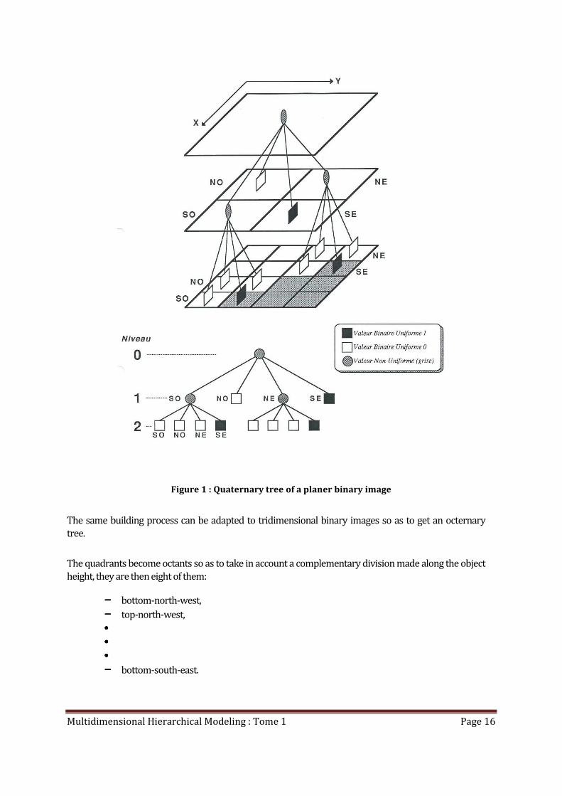
The underneath figure illustrates this dividing process and is showing that a graph of outer degree 4
(children number of a node) is generated in such a way: a quaternary tree.
Multidimensional Hierarchical Modeling : Tome 1 Page 16
Figure 1 : Quaternary tree of a planer binary image
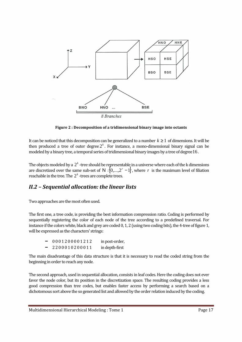
The same building process can be adapted to tridimensional binary images so as to get an octernary
tree.
The quadrants become octants so as to take in account a complementary division made along the object
height, they are then eight of them:
−−−− bottom-north-west,
−−−− top-north-west,
••••
••••
••••
−−−− bottom-south-east.
Multidimensional Hierarchical Modeling : Tome 1 Page 17
Figure 2 : Decomposition of a tridimensional binary image into octants
It can be noticed that this decomposition can be generalized to a number 1≥k of dimensions. It will be
then produced a tree of outer degreek2 . For instance, a mono-dimensional binary signal can be
modeled by a binary tree, a temporal series of tridimensional binary images by a tree of degree16.
The objects modeled by a k2 -tree should be representable in a universe where each of the k dimensions
are discretized over the same sub-set of Ν :{ }12,...,0 −r, where r is the maximum level of filiation
reachable in the tree. The k2 -trees are complete trees.
II.2 – Sequential allocation: the linear lists
Two approaches are the most often used.
The first one, a tree code, is providing the best information compression ratio. Coding is performed by
sequentially registering the color of each node of the tree according to a predefined traversal. For
instance if the colors white, black and grey are coded 0, 1, 2 (using two coding bits), the 4-tree of figure 1,
will be expressed as the characters’ strings:
−−−− 0 0 0 1 2 0 0 0 0 1 2 1 2 in post-order,
−−−− 2 2 0 0 0 1 0 2 0 0 0 1 1 in depth-first
The main disadvantage of this data structure is that it is necessary to read the coded string from the
beginning in order to reach any node.
The second approach, used in sequential allocation, consists in leaf codes. Here the coding does not ever
favor the node color, but its position in the discretization space. The resulting coding provides a less
good compression than tree codes, but enables faster access by performing a search based on a
dichotomous sort above the so generated list and allowed by the order relation induced by the coding.

Multidimensional Hierarchical Modeling : Tome 1 Page 18
The coding alphabet used for the 4-trees is (0, 1, 2, 3, X}, where 0, 1, 2, 3 refer to the four quadrants of
decomposition and X the un-development of a terminal node at an intermediate level inside the tree.
Code generation is performed by duplication of the code of a non-terminal node to be decomposed and
concatenation of the quadrant number of decomposition. By noticing that the code of terminal nodes are
including those of their fathers, these ones are not kept in the resulting list. Restarting from the example
of figure 1, the leaf code produced according to this method would be, if (SO, NO, NE, SE} is coded by (0,
1, 2, 3) :
−−−− (03, 23, 3X} by coding black nodes,
−−−− (00, 01, 02, 1X, 20, 21, 22} by coding white nodes.
Each one of these lists are ordered according to used quaternary alphabet and the applied function of
composition. The processed trees are no more complete At the opposite, each node is including in its
coding the path that links it to the tree root. The quaternary coding has an octernary equivalent for
octernary trees
II.3 – Indexed allocation: the linked lists
In a tree, there are two partial order relations:
−−−− filiation order,
−−−− and sibling order.
The filiation order is usually implemented at first in tree-like lists.
If it is planned to manage a tree according this single order, it is necessary to allocate to each tree node,
as many filiation links as the maximum number of children that it may have.
For enabling only downwards moves, it will be needed:
−−−− two successors for a binary tree, usually named left and right sons
−−−− four successors for a 4-tree,
−−−− k2 successors for a k2 -tree.
For enabling also upwards moves, only one complementary pointer is needed whatever can be the tree:
a father link.
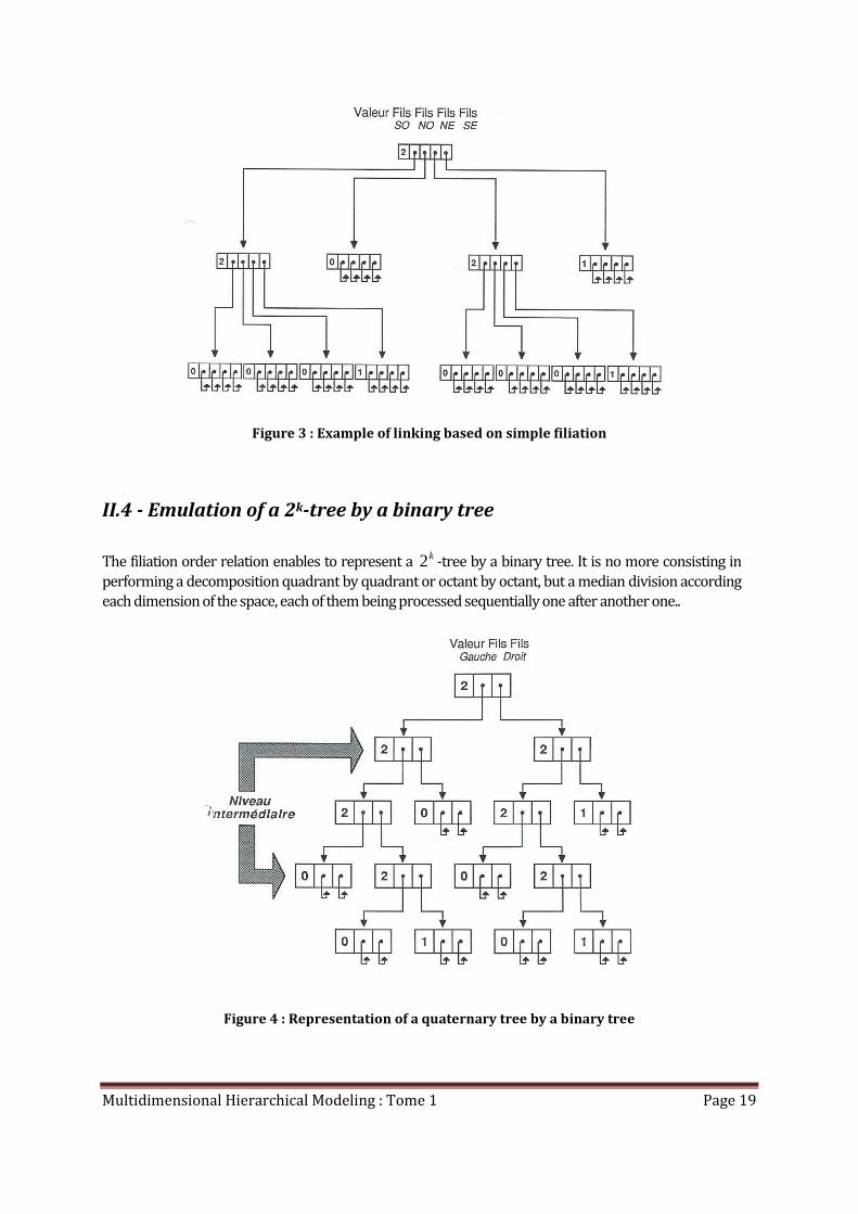
Restarting from the example of figure 1, it would be got the linked lists shown in figure 3. On this
example, it can be noticed that more than a half of memory usage is dedicated to the links of the children
of the terminal nodes. These data do not hold any meaning power and consist in a loss of memory space
but is necessary for insuring the consistency of the building. Usually, terminal nodes are implemented in
another way in order to minimize memory occupation.
Multidimensional Hierarchical Modeling : Tome 1 Page 19
Figure 3 : Example of linking based on simple filiation
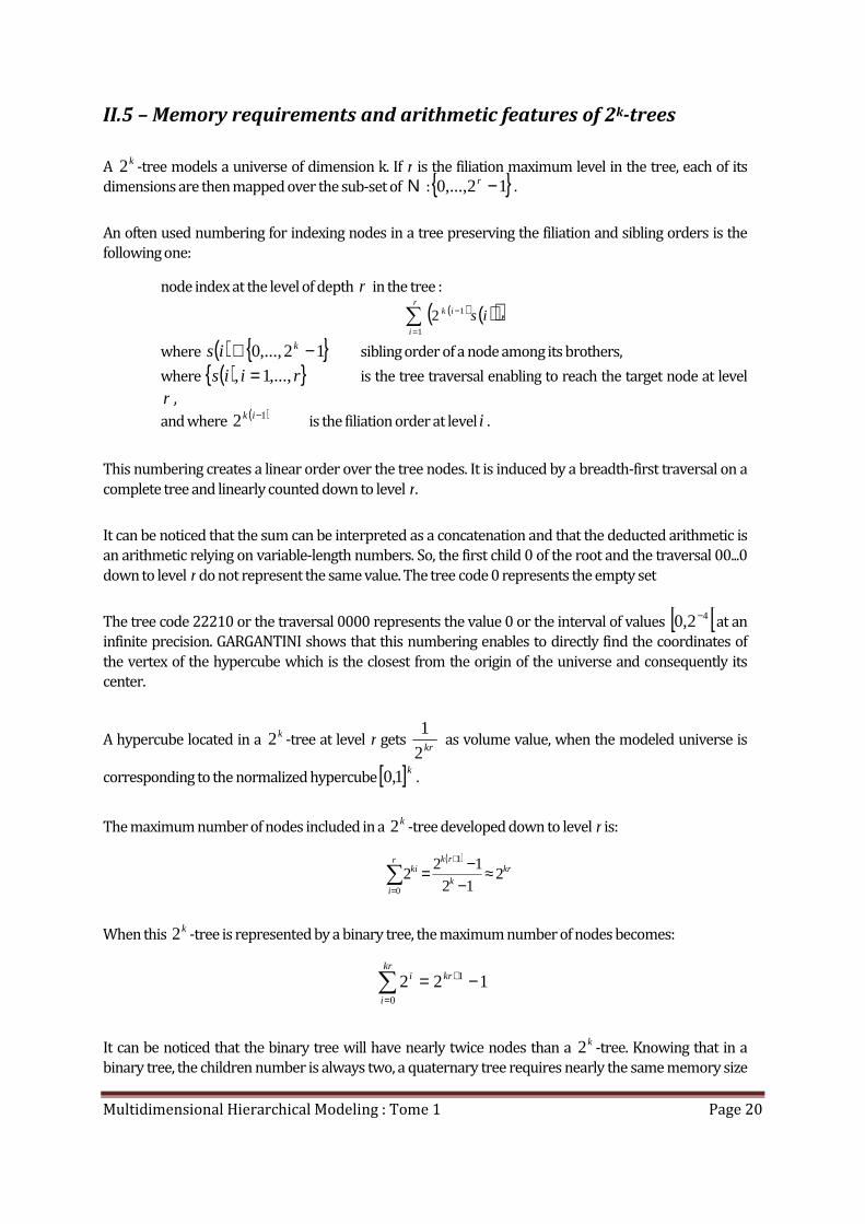
II.4 - Emulation of a 2k-tree by a binary tree
The filiation order relation enables to represent a k2 -tree by a binary tree. It is no more consisting in
performing a decomposition quadrant by quadrant or octant by octant, but a median division according
each dimension of the space, each of them being processed sequentially one after another one..
Figure 4 : Representation of a quaternary tree by a binary tree
Multidimensional Hierarchical Modeling : Tome 1 Page 20
II.5 – Memory requirements and arithmetic features of 2k-trees
A k2 -tree models a universe of dimension k. If r is the filiation maximum level in the tree, each of its
dimensions are then mapped over the sub-set of Ν :{ }12,...,0 −r.
An often used numbering for indexing nodes in a tree preserving the filiation and sibling orders is the
following one:
node index at the level of depth r in the tree :
( ) ( )( )∑=
−r
i
ik is1
12 ,
where ( ) { }12,...,0 −∈ kis sibling order of a node among its brothers,
where ( ){ }riis ,...,1, = is the tree traversal enabling to reach the target node at level
r ,
and where ( )12 −ik
is the filiation order at level i .
This numbering creates a linear order over the tree nodes. It is induced by a breadth-first traversal on a
complete tree and linearly counted down to level r.
It can be noticed that the sum can be interpreted as a concatenation and that the deducted arithmetic is
an arithmetic relying on variable-length numbers. So, the first child 0 of the root and the traversal 00...0
down to level r do not represent the same value. The tree code 0 represents the empty set
The tree code 22210 or the traversal 0000 represents the value 0 or the interval of values [ [42,0 −at an
infinite precision. GARGANTINI shows that this numbering enables to directly find the coordinates of
the vertex of the hypercube which is the closest from the origin of the universe and consequently its
center.
A hypercube located in a k2 -tree at level r gets
kr2
1 as volume value, when the modeled universe is
corresponding to the normalized hypercube[ ]k1,0 .
The maximum number of nodes included in a k2 -tree developed down to level r is:
( )kr
r
ik
rkki 2
12
122
0
1
≈−
−=∑=
+
When this k2 -tree is represented by a binary tree, the maximum number of nodes becomes:
∑=
+ −=kr
i
kri
0
1 122
It can be noticed that the binary tree will have nearly twice nodes than a k2 -tree. Knowing that in a
binary tree, the children number is always two, a quaternary tree requires nearly the same memory size
Multidimensional Hierarchical Modeling : Tome 1 Page 21
than its representation by a binary tree and, for any space of dimension k > 3, a binary tree will need less
memory than a k2 -tree implemented using a linked list.
II.6 – Geometric interpretation of 2k-trees
The k2 -trees are applied on multidimensional binary spaces. SRIHARI is seeing them as the
representation of the indicator function of objects belonging to the space to be modeled.
After having decomposed the corresponding space, this one appears as a set of unitary elements V
above which the modeled object is represented by the function { } { }1,0: →vf such as:
−−−− the object is the set ( ){ }1/ == vfvS ,
−−−− the background of the universe on which the object is described is the set
( ){ }0/ == vfvS .
So as to take in account multi-valued data, the representation can be extended to the following
formalism:
let nfff ,...,, 21 functionals defined on( )muuu ,...,, 21 , it can be defined the indicator function:
( ) ( )( ) { }1,0,...,,,...,,...,,,,...,,: 2121121 →mmmm uuufuuufuuuδ
where the value 1 is taken when the (m + n)-uplet exists and the value 0 at the opposite.
The set ( ){ }1/ == vvS δ will be the modeled numerical object and ( ){ }0/ == vvS δ the universe
background.
The tree-like modeling assumes that it is possible to regularly divide the object according each of these
dimensions:
−−−− either on the sub-set of the natural integers { }12...,,1,0 −r,
−−−− either on the sub-set of rational numbers
−
r
r
r 2
12...,,
2
1,0
or any variation between these two representations.
The function δ is then defined on the set approximated at the precision r
mn
r
r
r
+
−
2
12,...,
2
1,0 of
the unitary hypercube [ [ mn+1,0 .
By distinguishing no more the functionals from the variables on which they are applying, a k2 -tree will
describe an object belonging to the digital universe
k
r
r
r
−
2
12...,,
2
1,0
So a multilevel bi-dimensional image will have as indicator function:
( ) { }1,0min,, →escenceluyxδ and a 8-tree as model.
Multidimensional Hierarchical Modeling : Tome 1 Page 22
Likewise a colored bi-dimensional image will be similarly modeled by a 52 -tree so as to take in account
its three fundamental components.
To emulate a k2 -tree with a binary tree results to some modifications on this scheme. Actually the
support of the indicator function developed at the precision r is still not represented by the set :
k
r
r
r
−
2
12...,,
2
1,0 , but by
−
kr
kr
kr 2
12...,,
2
1,0
on the unitary segment [ [1,0 .
It is due to the fact that the division is not applied in parallel on the k dimensions of the space, but
sequentially one dimension after the other one. So the crossing from the precision r to 1+r is
performed by examining the k2 possible values of:
( )2/...,,2/,2/ 21 kuuu after having gone through those of the previous levels.
On a binary tree, this same operation consists in evaluating the number:
kkuuuu 2/...2/2/ 2
21 +++= .
A node index located at the precision r in the tree will get as value in a k2 -tree:
( ) ( )( )∑=
−r
i
ik is1
12
where ( ) { }12...,,0 −∈ kis is the sibling order of a node among its brothers ;
and where ( )12 −ik
is the filiation order at level i .
In the case of a binary tree, the node index at the depth r will have as value:
( )( )∑=
r
i
i is1
2 where ( ) { }1,0∈is
II.7 – Editing distance between trees
The problem is settled in a lexicographic manner by calculating the minimal cost enabling to transform a
tree A into a new one B. At each tree node is associated a label, and for editing a tree, only three
operations are allowed:
−−−− change the label of a tree node,
−−−− insert a sub-tree into a tree,
−−−− delete a sub-tree from a tree.
Each operation gets a positive cost.
Multidimensional Hierarchical Modeling : Tome 1 Page 23
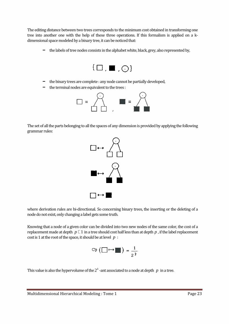
The editing distance between two trees corresponds to the minimum cost obtained in transforming one
tree into another one with the help of these three operations. If this formalism is applied on a k-
dimensional space modeled by a binary tree, it can be noticed that:
−−−− the labels of tree nodes consists in the alphabet white, black, grey, also represented by,
−−−− the binary trees are complete : any node cannot be partially developed,
−−−− the terminal nodes are equivalent to the trees :
The set of all the parts belonging to all the spaces of any dimension is provided by applying the following
grammar rules:
where derivation rules are bi-directional. So concerning binary trees, the inserting or the deleting of a
node do not exist, only changing a label gets some truth.
Knowing that a node of a given color can be divided into two new nodes of the same color, the cost of a
replacement made at depth 1+p in a tree should cost half less than at depth p , if the label replacement
cost is 1 at the root of the space, it should be at level p :
This value is also the hypervolume of thek2 -ant associated to a node at depth p in a tree.

Multidimensional Hierarchical Modeling : Tome 1 Page 24
Knowing that the binary trees are sentences of infinite length and that it is consequently possible to
directly compare them node by node, the minimal cost transform is unique, it is the one that changes
node by node the labels of differently colored nodes between them along a parallel traversal of the two
trees.
Concerning the replacement cost described above, the cost of this transform is equal to the mass of the
exclusive or of the two modeled sets, that is also the Lebesgue measure of the difference of the two sets
in another words the Hausdorff distance applied on sets modeled by k2 -trees :
( )BABAd ⊕= (), µ
That is also the weighted extension of the Hamming distance applied on tree codes.
The topology induced by the k2 -trees is less thin than the metric topologies commonly used. In fact if
the values 0 and 1/8 have got 1/8 as distance measure, the values 3/8 and 4/8 or 2/8 and 5/8 will get
7/8 as distance measure. It is only depending on the height of the common ancestor of these values in a
tree, which is providing the property of ultrametricity to this distance.
The Hausdorff distance is an ultrametric distance that does not enable to measure the distance between
two points of a space, but the distance between two parts of this same space.
Multidimensional Hierarchical Modeling : Tome 1 Page 25
III – Generation of trees modeling multidimensional data sets
III.1 - Representation of a vector
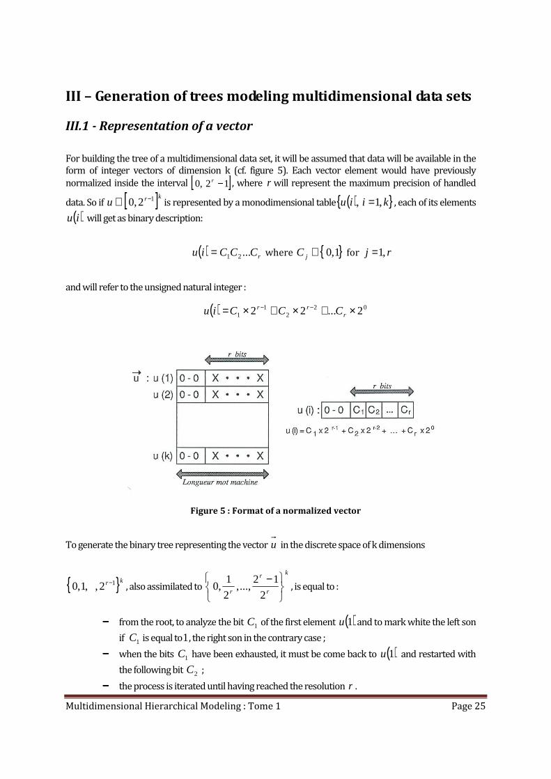
For building the tree of a multidimensional data set, it will be assumed that data will be available in the
form of integer vectors of dimension k (cf. figure 5). Each vector element would have previously
normalized inside the interval [ ]12,0 −r , where r will represent the maximum precision of handled
data. So if [ ]kru 12,0 −∈ is represented by a monodimensional table ( ){ }kiiu ,1, = , each of its elements
( )iu will get as binary description:
( ) rCCCiu ...21= where { }1,0∈jC for rj ,1=
and will refer to the unsigned natural integer :
( ) 022
11 2...22 ×+×+×= −−
rrr CCCiu
Figure 5 : Format of a normalized vector
To generate the binary tree representing the vector u in the discrete space of k dimensions
{ }kr 12,,1,0 −, also assimilated to
k
r
r
r
−
2
12...,,
2
1,0 , is equal to :
−−−− from the root, to analyze the bit 1C of the first element ( )1u and to mark white the left son
if 1C is equal to1, the right son in the contrary case ;
−−−− when the bits 1C have been exhausted, it must be come back to ( )1u and restarted with
the following bit 2C ;
−−−− the process is iterated until having reached the resolution r .
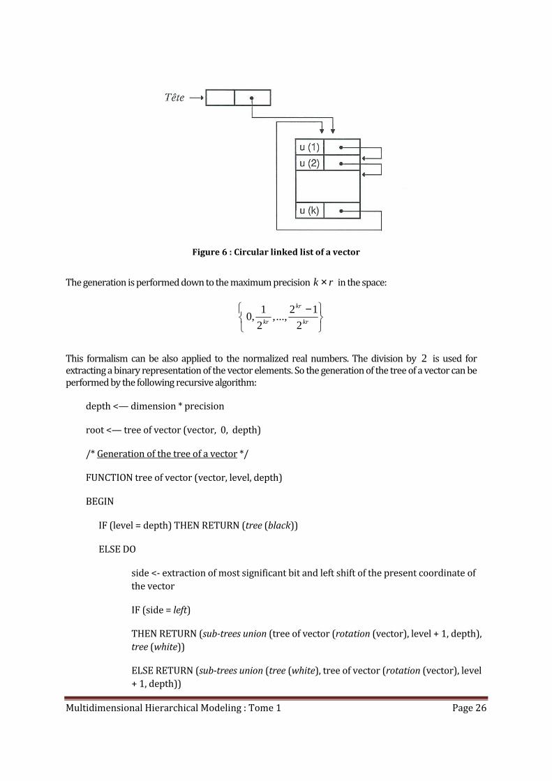
Multidimensional Hierarchical Modeling : Tome 1 Page 26
Figure 6 : Circular linked list of a vector
The generation is performed down to the maximum precision rk × in the space:
−
kr
kr
kr 2
12...,,
2
1,0
This formalism can be also applied to the normalized real numbers. The division by 2 is used for
extracting a binary representation of the vector elements. So the generation of the tree of a vector can be
performed by the following recursive algorithm:
depth <— dimension * precision
root <— tree of vector (vector, 0, depth)
/* Generation of the tree of a vector */
FUNCTION tree of vector (vector, level, depth)
BEGIN
IF (level = depth) THEN RETURN (tree (black))
ELSE DO
side <- extraction of most significant bit and left shift of the present coordinate of
the vector
IF (side = left)
THEN RETURN (sub-trees union (tree of vector (rotation (vector), level + 1, depth),
tree (white))
ELSE RETURN (sub-trees union (tree (white), tree of vector (rotation (vector), level
+ 1, depth))
Multidimensional Hierarchical Modeling : Tome 1 Page 27
END
END
III.2 - Generation of the tree of a set of vectors
By modifying the previous algorithm, it is possible to generate the tree modeling a set of vectors. Each
vector represents a realization of the indicator function that has been previously described. That is to
say that a vector ( )kuuuu ...,,, 21= will be an element of ( ){ }1/ == uuS δ .
The new proposed algorithm does not create the tree of a vector, but enriches an existing tree with the
realizations of a set of vectors. Enriching this structure consists in generating the path or the part of the
path, which is still described in the tree, when the circular list of a vector is analyzed.
The initialization of a tree generation is performed by creating a white colored tree. This procedure
generates a tree with only two white nodes, which is the set ( ){ }0/ =∀= uuU δ and which is
representing the empty universe of any dimension and at any precision. The initialization implies that
whatever is S , any path belonging to S is already registered in the tree. So only the black paths that are
still not described should be generated.
The merging of black symmetrical paths, on the return of recursive calls, enables to aggregate the
uniformly colored nodes.
root <- tree (white)
depth <- dimension * precision
CALL addition of a vector (root, vector, 0, depth)
/* Addition of a vector to a tree */
PROCEDURE addition of a vector (root, vector, level, depth)
BEGIN
IF (level = depth) ALORS blackening (root)
ELSE DO
side <- extraction of most significant bit and left shift of the current coordinate of the
vector
IF (terminal (root)) THEN fission (root)
CALL addition of a vector (child (root, side), rotation (vector), level + 1, depth)
merge (root)
END
Multidimensional Hierarchical Modeling : Tome 1 Page 28
END
This procedure of generation of the tree of a multidimensional data set by enriching a structure shows
different advantages:
−−−− it enables to take in account overcrowded data sets ;
−−−− it is compatible with ordered or not data flows.
III.3 – Tree access operators and associated algorithmic
The algorithmic applied on k2 -trees, which is followed, is built on the recursive calculus. It takes in favor
depth-first traversal of tree-like structures. It follows the definition of a tree proposed by KNUTH who
was understanding it as the recursive concatenation of sub-trees. So any recursive operator will fit to the
root of a tree, as well as to each of its nodes.
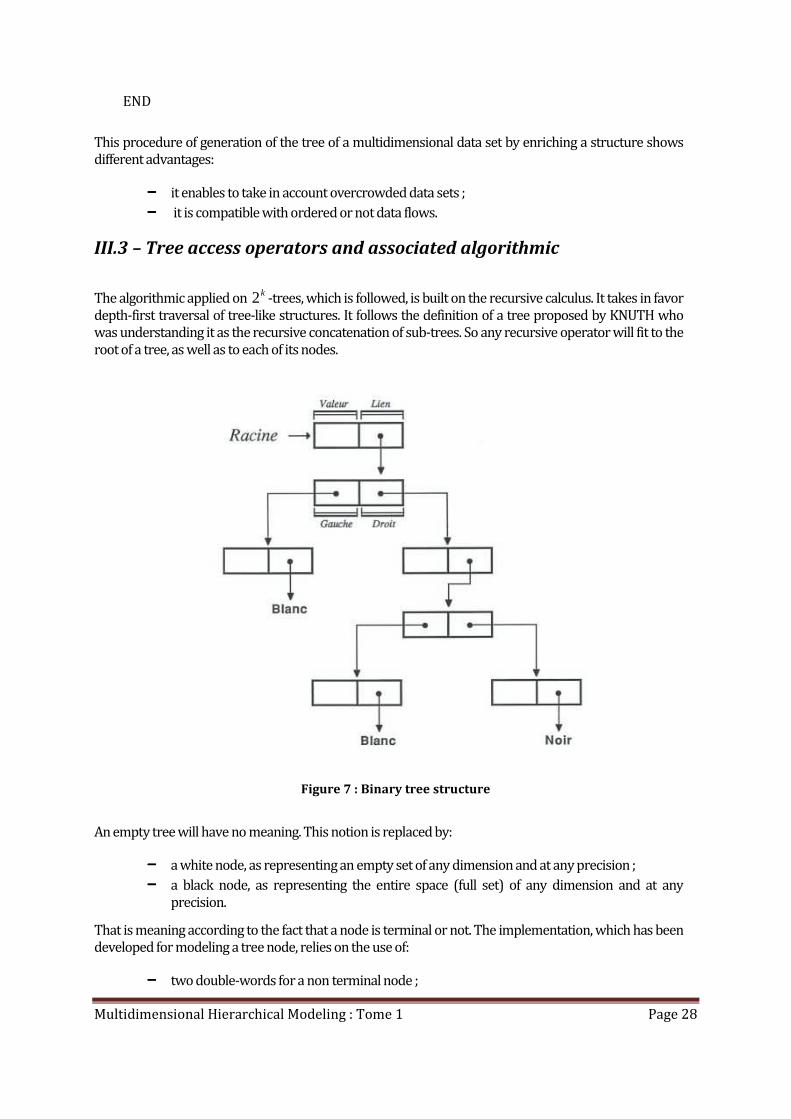
Figure 7 : Binary tree structure
An empty tree will have no meaning. This notion is replaced by:
−−−− a white node, as representing an empty set of any dimension and at any precision ;
−−−− a black node, as representing the entire space (full set) of any dimension and at any
precision.
That is meaning according to the fact that a node is terminal or not. The implementation, which has been
developed for modeling a tree node, relies on the use of:
−−−− two double-words for a non terminal node ;

Multidimensional Hierarchical Modeling : Tome 1 Page 29
−−−− a single double-word for a terminal node.
The first double-word is holding the addresses of the left and right sons of a node (the sub-trees).
Concerning a terminal node, this second word is useless because the white and black addresses are
auto-referring in the implemented addressing system. Knowing that any node in a tree is the root of a
new tree, it will be applied the word of root for appointing the address of a node in a tree.
For processing trees, it will be used depth-first traversals. So, the provision of a tree according to
whichever used operator can be performed with only two complementary ways:
−−−− by node fission, if the generation is performed during the descent of recursive calls ;
−−−− by node merge, if the generation is performed during the return of recursive calls.
A node deletion in a tree does not exist as it. It is replaced by the removal of the children sub-trees and
the setting at terminal state of the father node.
In addition, so as to minimize the extension of a tree, a merging operator enables to transform a tree in
which the two sons are iso-colored into a terminal node of the same color.
The it is possible to make an analogy between classical list operators and those that can apply on binary
trees, this one is shown in the table underneath.
List operators Tree operators
Create a list Create a tree of a given color (white/black)
Is empty a list? Is terminal a node ?
Next in the list Child of a given side (left/right)
Insert an element in a list Fission of a node into two others or union of two sub-trees
Delete an element in a list Merge a non terminal node
Delete a list Destruction of a tree
Table 1 : Correspondence between list and tree operators
III.4 – Boolean operations on trees
A lot of algorithms implementing Boolean operations on 4-trees or 8-trees have been published. The
Boolean operations on k2 -trees are performed according to the rules of the set theory.
Multidimensional Hierarchical Modeling : Tome 1 Page 30
Let be two k-dimensional sets 1S and 2S , represented by the binary trees, )( 1Stree and ( )2Stree . The
Boolean operations « and », « or », « exclusive or » and « not » are defined according to the following
manner:
−−−− )( 1Stree and ( )2Stree )( 3Stree→ / 213 SSS ∩=
−−−− )( 1Stree or ( )2Stree )( 3Stree→ / 213 SSS ∪=
−−−− )( 1Stree xor ( )2Stree )( 3Stree→ ) / 213 SSS ⊕=
−−−− not )( 1Stree )( 3Stree→ / 13 SS =
When the sets are representing objects of k dimensions, the Boolean operation "and" will perform the
intersection of the hypervolumes describing the objects, the operation "or" their union.
As terminal nodes of a binary tree have been implemented using auto-referring values, no troubles will
appear when paths of unequal lengths will be compared between two trees. This feature enables to
compare two trees built with two different precisions and to produce a new tree at a precision that can
be once more different from its operands. It makes available in addition to provide an assertion operator
that builds a copy of the operand tree but at a different precision from that used for its generation.
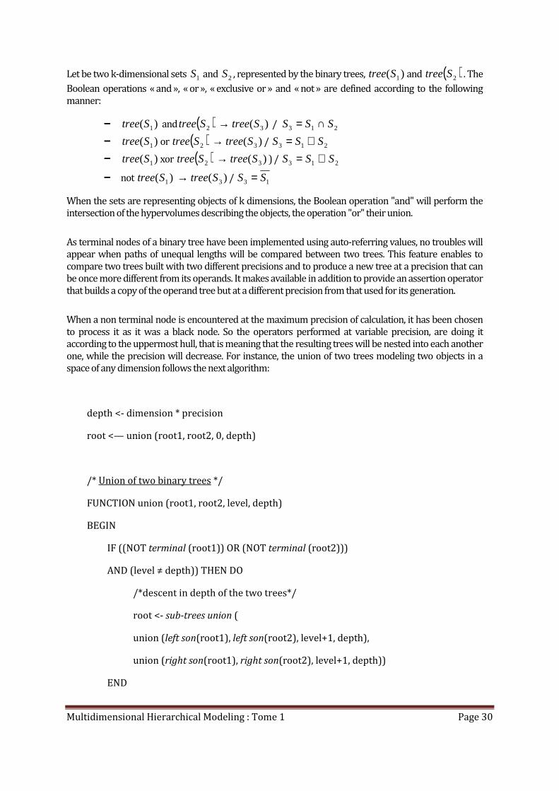
When a non terminal node is encountered at the maximum precision of calculation, it has been chosen
to process it as it was a black node. So the operators performed at variable precision, are doing it
according to the uppermost hull, that is meaning that the resulting trees will be nested into each another
one, while the precision will decrease. For instance, the union of two trees modeling two objects in a
space of any dimension follows the next algorithm:
depth <- dimension * precision
root <— union (root1, root2, 0, depth)
/* Union of two binary trees */
FUNCTION union (root1, root2, level, depth)
BEGIN
IF ((NOT terminal (root1)) OR (NOT terminal (root2)))
AND (level ≠ depth)) THEN DO
/*descent in depth of the two trees*/
root <- sub-trees union (
union (left son(root1), left son(root2), level+1, depth),
union (right son(root1), right son(root2), level+1, depth))
END

Multidimensional Hierarchical Modeling : Tome 1 Page 31
ELSE DO
/*union of the two reached nodes*/
IF ((white(root1)) AND (white(root2)))
THEN RETURN (tree (white))
ELSE RETURN (tree (black))
END
/*merge of children nodes when going up in the tree*/
merge (root)
RETURN (root)
END
III.5 – Inductive limit computations
In order to implement a procedure that will preserve the topological organization and the ability of
directly comparing trees between themselves, an initial topological structuring must be defined over the
spaces including any data of kR .
At first, it must be noticed that using a tree for modeling a data set of [ ]k1,0 , it leads to give it a structure
of Borel algebra. This structure is built on the atoms made from the k2 -ants resulting from the meshing
of [ ]k1,0 down to the precision r .
For each point of[ ]k1,0 , it can be combined a fundamental neighborhood system made from the atom
which is including it and the set of k2 -ants linked to the fatherly nodes of the tree branch which allows
to reach this node from the tree root: it will be got in such a way a series of nested parts whose union
will make up the unitary hypercube.
They are these fundamental neighborhood systems that, by symmetries analysis that they are sharing
between themselves, will enable to deduce from the modeled sets the properties that they are sharing
under the 1d and ∞d metric topologies and to transform them while respecting these ones.
Each k2 -ant of [ ]k1,0 whose precision is included between 1 and r , that is belonging to a branch of
the initial tree, makes up in its turn a Borel algebra down to an intermediate precision and is included in
the original Borel algebra and shares the same topology restricted to this sub-set.
Multidimensional Hierarchical Modeling : Tome 1 Page 32
In a similar manner, any algebra built as a union of an appropriate number of translated [ ]k1,0 so as
this one appears as homothetic to [ ]k1,0 will preserve once more the initial topology of[ ]k1,0 , deduced
from its neighborhood system.
So it can be propose an approach for building trees such as kR is the inductive limit of the algebras
homothetic to the unitary hypercube and such as the topologies of these algebras remain compliant
with those of their sub-algebras, that is meaning that a sub-algebra will always appear as a branch of the
tree of an algebra.
The implemented building method has been adapted from the tree generation by enrichment. The
approach is the following one, when a vector is added to an existing tree:
−−−− if the vector is not included in the initial space then the new bounds of the right space
holding the vector are computed an the tree is extended up to these new bounds ;
−−−− the vector is normalized according to these bounds, then added to the data already present
in the tree.
Computing new bounds, it is to determine the coordinates of the hypercube homothetic of a power of 2
of the previous hypercube, which is holding both this hypercube as well as the new data vector. These
coordinates are valued at:
−−−− in integer numbers :
{ }( )dxxdx iii /,min min,min, =
{ }( ) 11/,min max,max, −+= dxxdx iii
−−−− in real numbers :
{ } dxxdx iii /,min min,min, ⋅=
{ } dxxdx iii /,max max,max, ⋅=
−−−− where ( )ii xxd min,max,2log2 −= for { }ki ...,,1∈
−−−− where { } { }kiix ...,,1∈ is the data vector, and { } { }ii xx max,min, , the ends of the first diagonal of
the hypercube ;
−−−− and where et are the floor and ceiling operators for converting a floating point
number into an integer one.
These computations are implemented by an iterative procedure which is converging towards the
satisfying of these equalities.
The generation of a tree in inductive limit needs to keep always some complementary information: the
bounds of the space in which has been built the k2 -tree. These bounds are the vertices of the hypercube
of the tree decomposition, which is also the referring hypercube of the set modeled by the tree.
Until now the k2 -trees have always been built in the unitary hypercube of the space at k dimensions.
Building in inductive limit enables to build trees in any translated of a homothetic copy of the unitary
hypercube. For actually comparing two trees generated into two different referring hypercubes, it is
necessary to know these ones.

Multidimensional Hierarchical Modeling : Tome 1 Page 33
When the k2 -trees are brought together with their referring hypercubes, then it can be performed
Boolean operations on them, even if their hypercubes are not equal. By comparison of the operand
referring hypercubes, it can be know which hypercube is including them and how to extend the
operands to this new hypercube. The two trees having been extended up to this new space, the Boolean
operation is applied and provides a resulting tree which referring hypercube is the hypercube
computed from those belonging to the operands.

Multidimensional Hierarchical Modeling : Tome 1 Page 34
Multidimensional Hierarchical Modeling : Tome 1 Page 35
IV – Geometric transforms
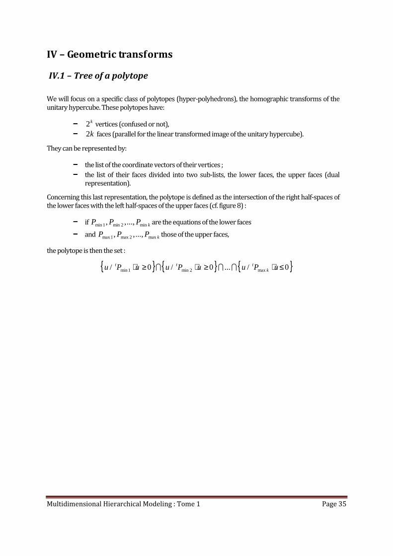
IV.1 – Tree of a polytope
We will focus on a specific class of polytopes (hyper-polyhedrons), the homographic transforms of the
unitary hypercube. These polytopes have:
−−−− k2 vertices (confused or not),
−−−− k2 faces (parallel for the linear transformed image of the unitary hypercube).
They can be represented by:
−−−− the list of the coordinate vectors of their vertices ;
−−−− the list of their faces divided into two sub-lists, the lower faces, the upper faces (dual
representation).
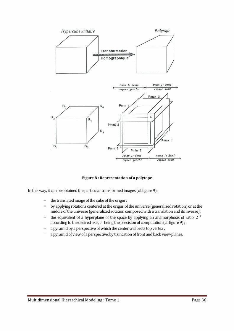
Concerning this last representation, the polytope is defined as the intersection of the right half-spaces of
the lower faces with the left half-spaces of the upper faces (cf. figure 8) :
−−−− if kPPP min2min1min ...,,, are the equations of the lower faces
−−−− and kPPP max2max1max ...,,, those of the upper faces,
the polytope is then the set :
{ } { } { }0/...0/0/ max2min1min ≤⋅≥⋅≥⋅ uPuuPuuPu kttt
III
Multidimensional Hierarchical Modeling : Tome 1 Page 36
Figure 8 : Representation of a polytope
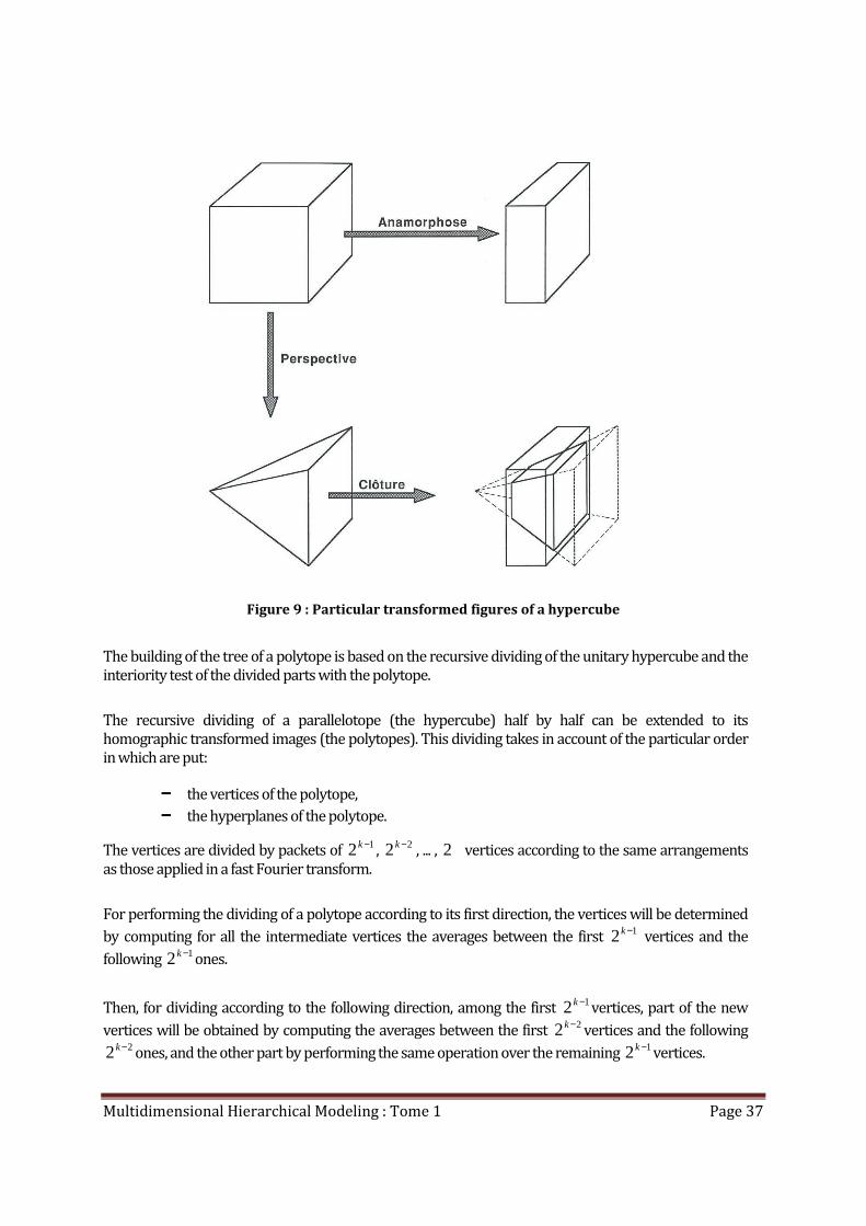
In this way, it can be obtained the particular transformed images (cf. figure 9):
−−−− the translated image of the cube of the origin ;
−−−− by applying rotations centered at the origin of the universe (generalized rotation) or at the
middle of the universe (generalized rotation composed with a translation and its inverse) ;
−−−− the equivalent of a hyperplane of the space by applying an anamorphosis of ratio r−2
according to the desired axis, r being the precision of computation (cf. figure 9) ;
−−−− a pyramid by a perspective of which the center will be its top vertex ;
−−−− a pyramid of view of a perspective, by truncation of front and back view-planes.
Multidimensional Hierarchical Modeling : Tome 1 Page 37
Figure 9 : Particular transformed figures of a hypercube
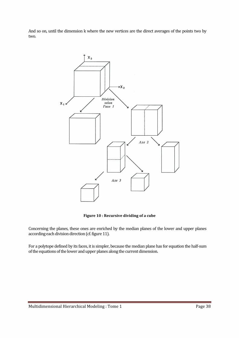
The building of the tree of a polytope is based on the recursive dividing of the unitary hypercube and the
interiority test of the divided parts with the polytope.
The recursive dividing of a parallelotope (the hypercube) half by half can be extended to its
homographic transformed images (the polytopes). This dividing takes in account of the particular order
in which are put:
−−−− the vertices of the polytope,
−−−− the hyperplanes of the polytope.
The vertices are divided by packets of 12 −k,
22 −k, ... , 2 vertices according to the same arrangements
as those applied in a fast Fourier transform.
For performing the dividing of a polytope according to its first direction, the vertices will be determined
by computing for all the intermediate vertices the averages between the first 12 −k vertices and the
following 12 −kones.
Then, for dividing according to the following direction, among the first 12 −kvertices, part of the new
vertices will be obtained by computing the averages between the first 22 −k
vertices and the following 22 −k
ones, and the other part by performing the same operation over the remaining 12 −kvertices.
Multidimensional Hierarchical Modeling : Tome 1 Page 38
And so on, until the dimension k where the new vertices are the direct averages of the points two by
two.
Figure 10 : Recursive dividing of a cube
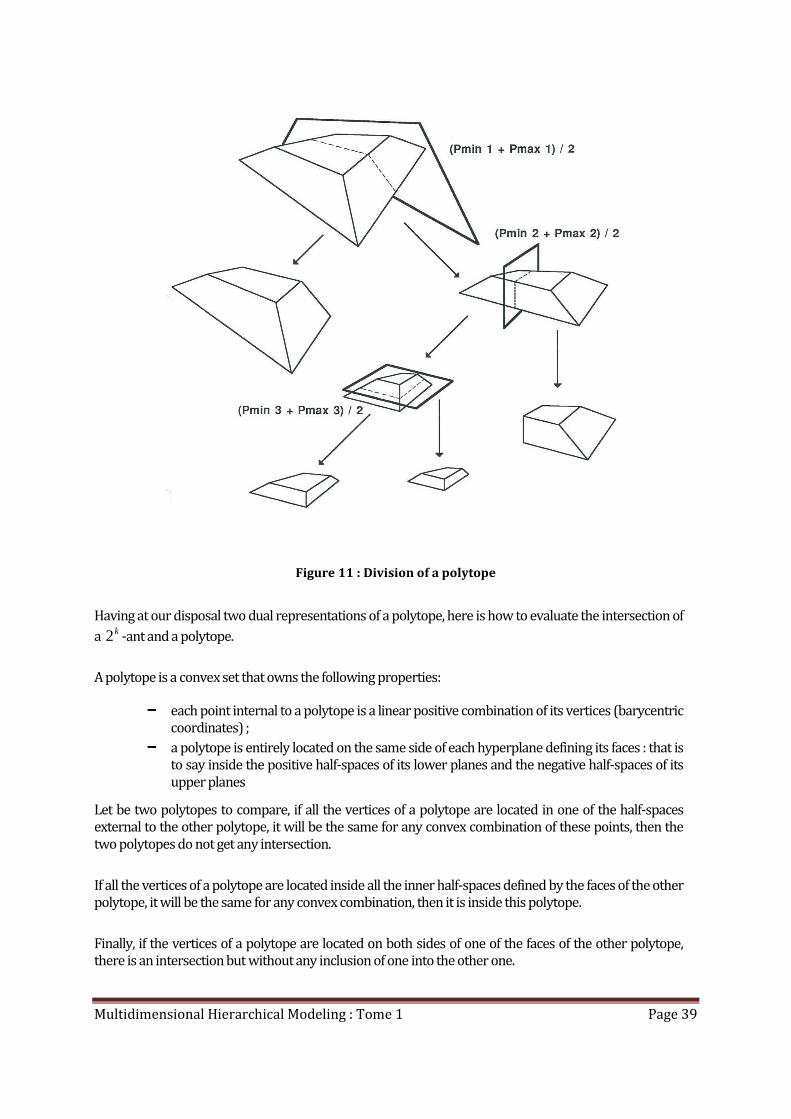
Concerning the planes, these ones are enriched by the median planes of the lower and upper planes
according each division direction (cf. figure 11).
For a polytope defined by its faces, it is simpler, because the median plane has for equation the half-sum
of the equations of the lower and upper planes along the current dimension.
Multidimensional Hierarchical Modeling : Tome 1 Page 39
Figure 11 : Division of a polytope
Having at our disposal two dual representations of a polytope, here is how to evaluate the intersection of
a k2 -ant and a polytope.
A polytope is a convex set that owns the following properties:
−−−− each point internal to a polytope is a linear positive combination of its vertices (barycentric
coordinates) ;
−−−− a polytope is entirely located on the same side of each hyperplane defining its faces : that is
to say inside the positive half-spaces of its lower planes and the negative half-spaces of its
upper planes
Let be two polytopes to compare, if all the vertices of a polytope are located in one of the half-spaces
external to the other polytope, it will be the same for any convex combination of these points, then the
two polytopes do not get any intersection.
If all the vertices of a polytope are located inside all the inner half-spaces defined by the faces of the other
polytope, it will be the same for any convex combination, then it is inside this polytope.
Finally, if the vertices of a polytope are located on both sides of one of the faces of the other polytope,
there is an intersection but without any inclusion of one into the other one.
Multidimensional Hierarchical Modeling : Tome 1 Page 40
By recursively dividing the unitary hypercube and comparing the result with the initial polytope, it can
be directly generated the tree of this polytope while coloring in black the inclusions, in grey the
intersections to be developed and in white the lacks of intersection.
IV.2 – Homographic transformation of a 2k-tree
Analytically, a hyperplane is the set of points:
{ }∗∈=⋅∈ EvuvEu t ,0/
i.e., by decomposing u in its reference system and v in its dual basis:
∈=⋅∈ ∑=
∗
kiii EvuvEu
,1
,0,
One of the main interests of this analytic representation is the following one: if a bijective map f is
applied on a set of points E , it is equivalent to perform the inverse map 1−f on
∗E .
So the homographic transformed image of a polytope gets:
−−−− as vertices, the direct transformed images of its vertices ;
−−−− as faces, the inverse transformed images of the parametric expressions of its faces.
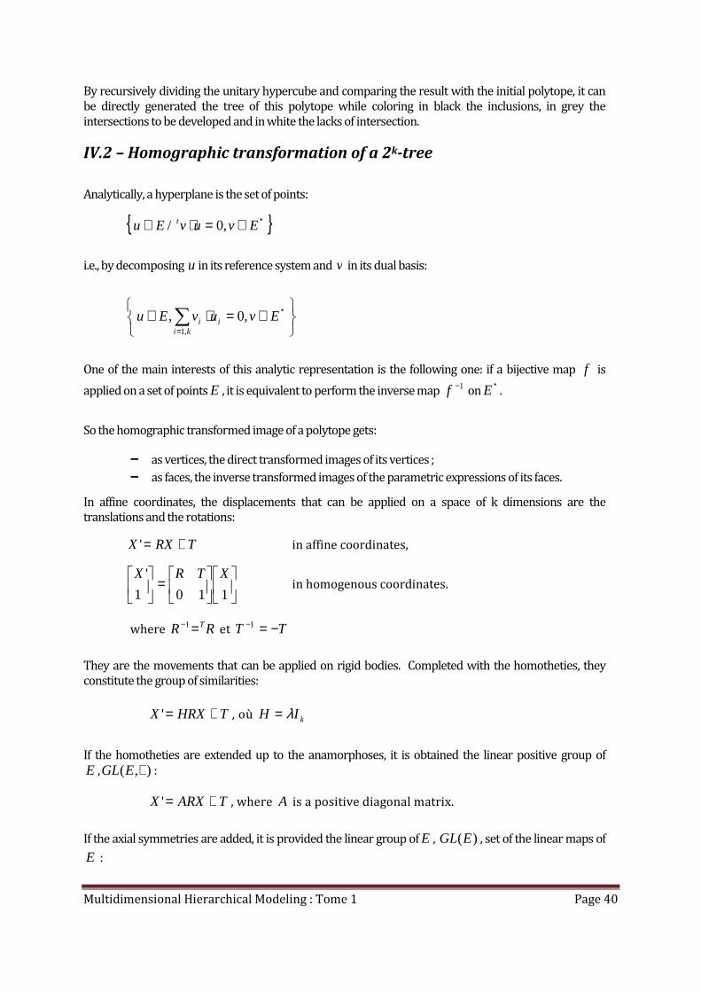
In affine coordinates, the displacements that can be applied on a space of k dimensions are the
translations and the rotations:
TRXX +=' in affine coordinates,
=
1101
' XTRX in homogenous coordinates.
where RR T=−1 et TT −=−1
They are the movements that can be applied on rigid bodies. Completed with the homotheties, they
constitute the group of similarities:
THRXX +=' , où kIH λ=
If the homotheties are extended up to the anamorphoses, it is obtained the linear positive group of
E , ),( +EGL :
TARXX +=' , where A is a positive diagonal matrix.
If the axial symmetries are added, it is provided the linear group of E , )(EGL , set of the linear maps of
E :
Multidimensional Hierarchical Modeling : Tome 1 Page 41
TARXX +=' , where kIS =2, i.e. SS =−1
If the space is described in homogenous coordinates, the linear group, completed with perspectives,
constitutes the projective linear group )(EPGL :
=
W
X
P
TSAR
W
XT 1'
', where PP −=−1
It gathers all the maps en in homogenous coordinates that can be applied on E , the maps being
geometrically together equivalent by a multiplicative factor. They are homographies.
For a space described in affine coordinates, the homographic transformations are not linear. They are
needing at the end of a transformation to normalize the homogenous coordinates with the help of the
weight of the (k+1)-th coordinate in order to able to come back to affine coordinates.
The process of recursive dividing of a polytope can be also applied on the calculation of the homographic
transformation of a tree. Actually, the middle of a line segment is in harmonic division with the ends of
this line segment and the point at the infinite according to the direction of the line segment (their cross-
ratio is valued at 1− ). The cross-ratio of four points remains unchanged by any homography.
By duality, two hyperplanes, their median hyperplane and the hyperplane at the infinite constitute a
harmonic bundle.
Then there will be an equivalence between the homographic images of the decompositions of an
hypercube and the recursive decompositions of the homographic image of the same hypercube.
To avoid the computation of the homographic transformed images of k2 -ants inside the initial space, it
can be noticed that it will be got a same tree as the tree of the transformed set by decomposing the initial
set into the inverse image of the unitary hypercube of the image space. Actually, the vertices of a regular
division of the unitary hypercube of the image space and their inverse images will be in bijective
correspondence for this transformation.
For computing the image tree resulting from this transform, it is then equal to decompose the
transformed set inside the unitary cube as well as to decompose the initial set inside the inverse image
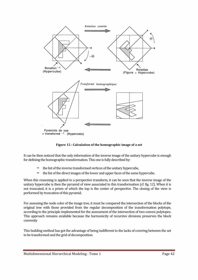
of this same cube. For instance, the figure 12 shows this fact for a rotation of a given angle: the
decomposition of the transformed image by the given rotation is bijective with the decomposition of the
initial set in the inverse image of the unitary hypercube (bijection enlightened by the hatched part in a
same quadrant of decomposition).
Multidimensional Hierarchical Modeling : Tome 1 Page 42
Figure 12 : Calculation of the homographic image of a set
It can be then noticed that the only information of the inverse image of the unitary hypercube is enough
for defining the homographic transformation. This one is fully described by:
−−−− the list of the inverse transformed vertices of the unitary hypercube,
−−−− the list of the direct images of the lower and upper faces of the same hypercube.
When this reasoning is applied to a perspective transform, it can be seen that the inverse image of the
unitary hypercube is then the pyramid of view associated to this transformation (cf. fig. 12). When it is
not truncated, it is a prism of which the top is the center of perspective. The closing of the view is
performed by truncation of this pyramid.
For assessing the node color of the image tree, it must be compared the intersection of the blocks of the
original tree with those provided from the regular decomposition of the transformation polytope,
according to the principle implemented for the assessment of the intersection of two convex polytopes.
This approach remains available because the harmonicity of recursive divisions preserves the block
convexity
This building method has got the advantage of being indifferent to the lacks of covering between the set
to be transformed and the grid of decomposition.

Multidimensional Hierarchical Modeling : Tome 1 Page 43
Finally, the calculation of the homographic image starts with the building of the tree of the transformed
polytope. The building is driven by the search of common black nodes between the set to be
transformed and the tree of the transformed polytope, which is restricting the calculation of the
transformed image to the only nodes concerned by the transformation inside a tree of any precision.

Multidimensional Hierarchical Modeling : Tome 1 Page 44
Multidimensional Hierarchical Modeling : Tome 1 Page 45
V - Segmentation
V.1 – Adjacencies search
The concept of neighborhood in a metric space is relying on the use of a distance in this space. The most
commonly used distances are:
−−−− ( ) iiki
yxYXd −==∞
,1max, ,
−−−− ( ) ∑=
−=ki
ii yxYXd,1
1 , ,
−−−− ( )2
,12 ,
−= ∑
= kiii yxYXd , Euclidean distance.
Inside a meshed metric space, two points X and Y will be adjacent or neighbors, if they are distant of
one resolution unit of the space. That is to say that they must satisfy to the relation:
YX dℜ : YX ≠ and ( ) 1, ≤YXd in{ }kr 12...,,1,0 −,
or again :
YX dℜ : YX ≠ and ( )r
YXd2
1, ≤ in
k
r
r
r
−
2
12...,,
2
1,0 .
So the set of neighbors of X in { }kr 12...,,1,0 −will be the unitary ball:
( ) { } ( ){ }1,/12...,,1,01, ≤≠−∈= YXdetXYYXBkr
d ,
And in
k
r
r
r
−
2
12...,,
2
1,0 ,it will be the ball of highest resolution
rd XB
2
1, .
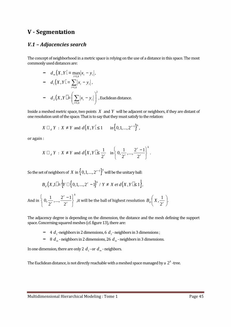
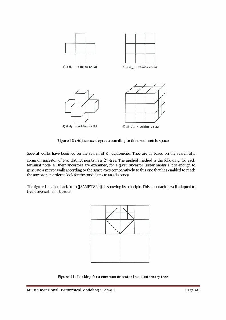
The adjacency degree is depending on the dimension, the distance and the mesh defining the support
space. Concerning squared meshes (cf. figure 13), there are:
−−−− 4 1d -neighbors in 2 dimensions, 6 1d - neighbors in 3 dimensions ;
−−−− 8 ∞d - neighbors in 2 dimensions, 26 ∞d - neighbors in 3 dimensions.
In one dimension, there are only 2 1d - or ∞d - neighbors.
The Euclidean distance, is not directly reachable with a meshed space managed by a k2 -tree.
Multidimensional Hierarchical Modeling : Tome 1 Page 46
Figure 13 : Adjacency degree according to the used metric space
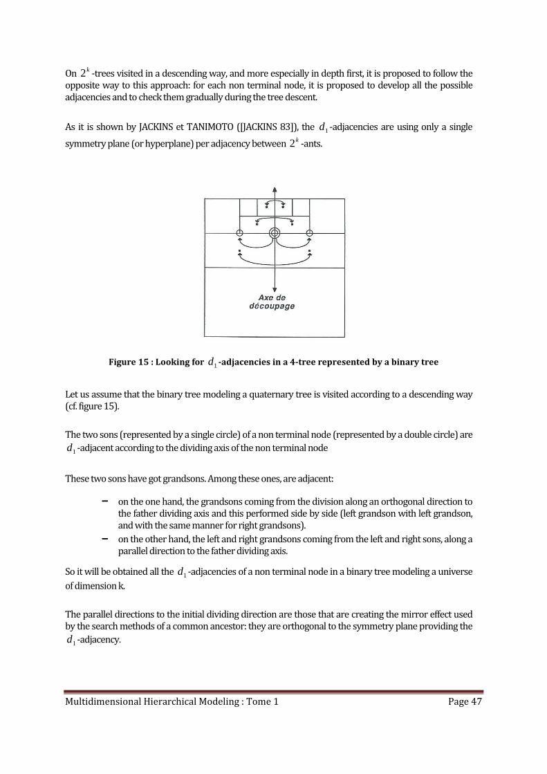
Several works have been led on the search of 1d -adjacencies. They are all based on the search of a
common ancestor of two distinct points in a k2 -tree. The applied method is the following: for each
terminal node, all their ancestors are examined, for a given ancestor under analysis it is enough to
generate a mirror walk according to the space axes comparatively to this one that has enabled to reach
the ancestor, in order to look for the candidates to an adjacency.
The figure 14, taken back from ([SAMET 82a]), is showing its principle. This approach is well adapted to
tree traversal in post-order.
Figure 14 : Looking for a common ancestor in a quaternary tree
Multidimensional Hierarchical Modeling : Tome 1 Page 47
On k2 -trees visited in a descending way, and more especially in depth first, it is proposed to follow the
opposite way to this approach: for each non terminal node, it is proposed to develop all the possible
adjacencies and to check them gradually during the tree descent.
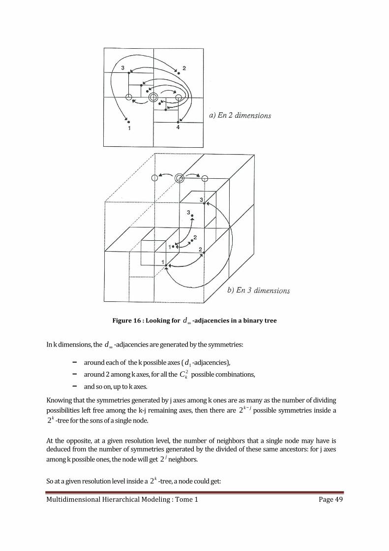
As it is shown by JACKINS et TANIMOTO ([JACKINS 83]), the 1d -adjacencies are using only a single
symmetry plane (or hyperplane) per adjacency between k2 -ants.
Figure 15 : Looking for 1d -adjacencies in a 4-tree represented by a binary tree
Let us assume that the binary tree modeling a quaternary tree is visited according to a descending way
(cf. figure 15).
The two sons (represented by a single circle) of a non terminal node (represented by a double circle) are
1d -adjacent according to the dividing axis of the non terminal node
These two sons have got grandsons. Among these ones, are adjacent:
−−−− on the one hand, the grandsons coming from the division along an orthogonal direction to
the father dividing axis and this performed side by side (left grandson with left grandson,
and with the same manner for right grandsons).
−−−− on the other hand, the left and right grandsons coming from the left and right sons, along a
parallel direction to the father dividing axis.
So it will be obtained all the 1d -adjacencies of a non terminal node in a binary tree modeling a universe
of dimension k.
The parallel directions to the initial dividing direction are those that are creating the mirror effect used
by the search methods of a common ancestor: they are orthogonal to the symmetry plane providing the
1d -adjacency.

Multidimensional Hierarchical Modeling : Tome 1 Page 48
Only SAMET has been interested in looking for ∞d -adjacencies and this study has been performed on
quaternary trees.
In a universe of dimension k, the ∞d -adjacencies are including the 1d -adjacencies, which is meaning
those produced by the adjacencies around a dividing axis among k possible ones. They can be
completed with the adjacencies created by the connections generated by two or more than two axes
among the k possible ones, that is to say by the combination of two or more than two symmetry planes
or hyperplanes.
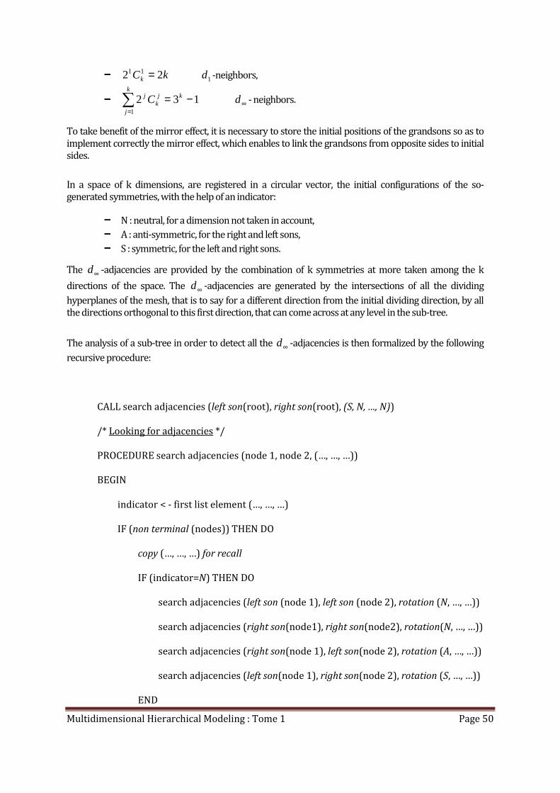
So, as it is shown on figure 16.a) in two dimensions:
−−−− after two dividing steps, the furthest nodes coming from the sons are adjacent;
−−−− all the grandsons, coming from a further division according to each of the two axes, are
adjacent, right and left grandsons coming from the left and right sons (mirror effect).
In three dimensions (cf. figure 16. b) ; the same situation occurs:
−−−− for the two diving axes (link 1 with 2), the third one does not play any role,
−−−− for the three axes (link 1 with 3),
−−−− and for the first and the last dimensions, even if it is not displayed on the figure.
Multidimensional Hierarchical Modeling : Tome 1 Page 49
Figure 16 : Looking for ∞d -adjacencies in a binary tree
In k dimensions, the ∞d -adjacencies are generated by the symmetries:
−−−− around each of the k possible axes ( 1d -adjacencies),
−−−− around 2 among k axes, for all the 2kC possible combinations,
−−−− and so on, up to k axes.
Knowing that the symmetries generated by j axes among k ones are as many as the number of dividing
possibilities left free among the k-j remaining axes, then there are jk −2 possible symmetries inside a
k2 -tree for the sons of a single node.
At the opposite, at a given resolution level, the number of neighbors that a single node may have is
deduced from the number of symmetries generated by the divided of these same ancestors: for j axes
among k possible ones, the node will get j2 neighbors.
So at a given resolution level inside a k2 -tree, a node could get:
Multidimensional Hierarchical Modeling : Tome 1 Page 50
−−−− kCk 22 11 = 1d -neighbors,
−−−− ∑=
−=k
j
kjk
j C1
132 ∞d - neighbors.
To take benefit of the mirror effect, it is necessary to store the initial positions of the grandsons so as to
implement correctly the mirror effect, which enables to link the grandsons from opposite sides to initial
sides.
In a space of k dimensions, are registered in a circular vector, the initial configurations of the so-
generated symmetries, with the help of an indicator:
−−−− N : neutral, for a dimension not taken in account,
−−−− A : anti-symmetric, for the right and left sons,
−−−− S : symmetric, for the left and right sons.
The ∞d -adjacencies are provided by the combination of k symmetries at more taken among the k
directions of the space. The ∞d -adjacencies are generated by the intersections of all the dividing
hyperplanes of the mesh, that is to say for a different direction from the initial dividing direction, by all
the directions orthogonal to this first direction, that can come across at any level in the sub-tree.
The analysis of a sub-tree in order to detect all the ∞d -adjacencies is then formalized by the following
recursive procedure:
CALL search adjacencies (left son(root), right son(root), (S, N, …, N))
/* Looking for adjacencies */
PROCEDURE search adjacencies (node 1, node 2, (…, …, …))
BEGIN
indicator < - first list element (…, …, …)
IF (non terminal (nodes)) THEN DO
copy (…, …, …) for recall
IF (indicator=N) THEN DO
search adjacencies (left son (node 1), left son (node 2), rotation (N, …, …))
search adjacencies (right son(node1), right son(node2), rotation(N, …, …))
search adjacencies (right son(node 1), left son(node 2), rotation (A, …, …))
search adjacencies (left son(node 1), right son(node 2), rotation (S, …, …))
END
Multidimensional Hierarchical Modeling : Tome 1 Page 51
IF (indicator=S) THEN
search adjacencies (right son(node 1), left son(node 2), rotation(S, …, …))
IF (indicator=A) THEN
search adjacencies (left son(node 1), right son(node 2), rotation(A, …, …))
restore stored vector
END
ELSE store the adjacencies of terminal nodes
END
It can be come back to the 1d -adjacencies by deleting the combinations of symmetry axes:
CALL search adjacencies (left son(root), right son(root), (S, N, …, N))
/* Looking for adjacencies */
PROCEDURE search adjacencies (node 1, node 2, (…, …, …))
BEGIN
indicator < - first list element (…, …, …)
IF (non terminal (nodes)) THEN DO
copy (…, …, …) for recall
IF (indicator=N) THEN DO
search adjacencies (left son (node 1), left son (node 2), rotation (N, …, …))
search adjacencies (right son(node1), right son(node2), rotation(N, …, …))
END
IF (indicator=S) THEN
search adjacencies (right son(node 1), left son(node 2), rotation(S, …, …))
restore stored vector
END
ELSE store the adjacencies of terminal nodes
END
Multidimensional Hierarchical Modeling : Tome 1 Page 52
V.2 - Labeling of connected components
Two adjacent points YX , , according to an unspecified distance, will be 1-connected. If there is a path of
n-1 adjacent points enabling to join X to Y , then X and Y will be n- connected.
A set of points will be a connected set, if whatever are two points X and Y belonging to this set, there is
a path of an unknown length enabling to join X to Y in this set. In other words, a set V will be
connected if :
⇔ℜ∈∀ YXVYX c,, either YX = ,
or { } 1,1 / ZXVZ cnii ℜ⊂∃ = , 1,1,1 −=ℜ + niZZ ici , YZ cn ℜ .
The relation of connectivity cℜ is an equivalence relation.
Let be V , some set, a partition of V is a decomposition of V into n separate sub-sets iV , as their union
reconstitutes V :
−−−− jiji ≠∀ /, ∅≠∩ ji VV ;
−−−− ini
VV ∪=
=,1
.
A predicate P will a Boolean function over the set of the parts of some set V :
{ }falsetrueVPP i ,)(: ∈ and VVi ⊂
A segmentation of V according to the predicate P is a partition { } niiV ,1= of V such as:
−−−− { } trueVPni i =∈∀ )(,1 ,
−−−− and { } falseVVPjinji ji =∪≠∈∀ )(,,1,
Let be ℜ an equivalence relation on V , an equivalence class of ℜ over the set V will be a sub-set ℜV of
V such as :
−−−− ℜ∈∀ VYX , YXV ℜ:
The set of the equivalence classes of a set V for a relation ℜ constitutes a partition of V .
The equivalence classes for the connectivity relation cℜ will be named connected components.
Knowing that a multidimensional discrete space can be represented by its indicator function
{ } { }1,0: →Vδ , it will be then provided a segmentation of V by the predicate P of iso-coloring :
trueVP =)( if )()(,, YXVYX δδ =∈∀ over the set of connected components of V .

Multidimensional Hierarchical Modeling : Tome 1 Page 53
The adjacency analysis having been performed on the binary tree modeling a space of k dimensions, it is
now possible to discover the connected components of this space and to label each terminal node with
the label of the component to which it is belonging.
Two algorithms have been designed for implementing a recursive labeling over k2 -trees. There is the
one developed by SAMET ([SAMET 81a]) which is relying on an algorithm described by ([KNUTH 73]),
and the other one developed by GARGANTINI ([GARGANTINI 82c])
The SAMET algorithm is based on the notion of adjacency tree.
The method followed by GARGANTINI is easier to deal with but not easily parallelisable. It relies on the
numbering of all the connected points belonging to a newly detected component:
−−−− when a new component is detected, it is loaded up with the point that has enabling its
discover and all its neighbors, and these ones are stored in a queue for their further
processing ;
−−−− when one point has been examined, it is checked if the queue is not empty, if it is true, the
next point to be examined is caught from the queue before looking for a new starting point
in the tree, in order to exhaust the former detected component).
At last, the tree being labeled, it is then possible to compute the list of the segment-trees, that is to extract
from the labeled tree, the trees of all the connected components and to link them into a single list : the
forest of the segment-trees.

Multidimensional Hierarchical Modeling : Tome 1 Page 54
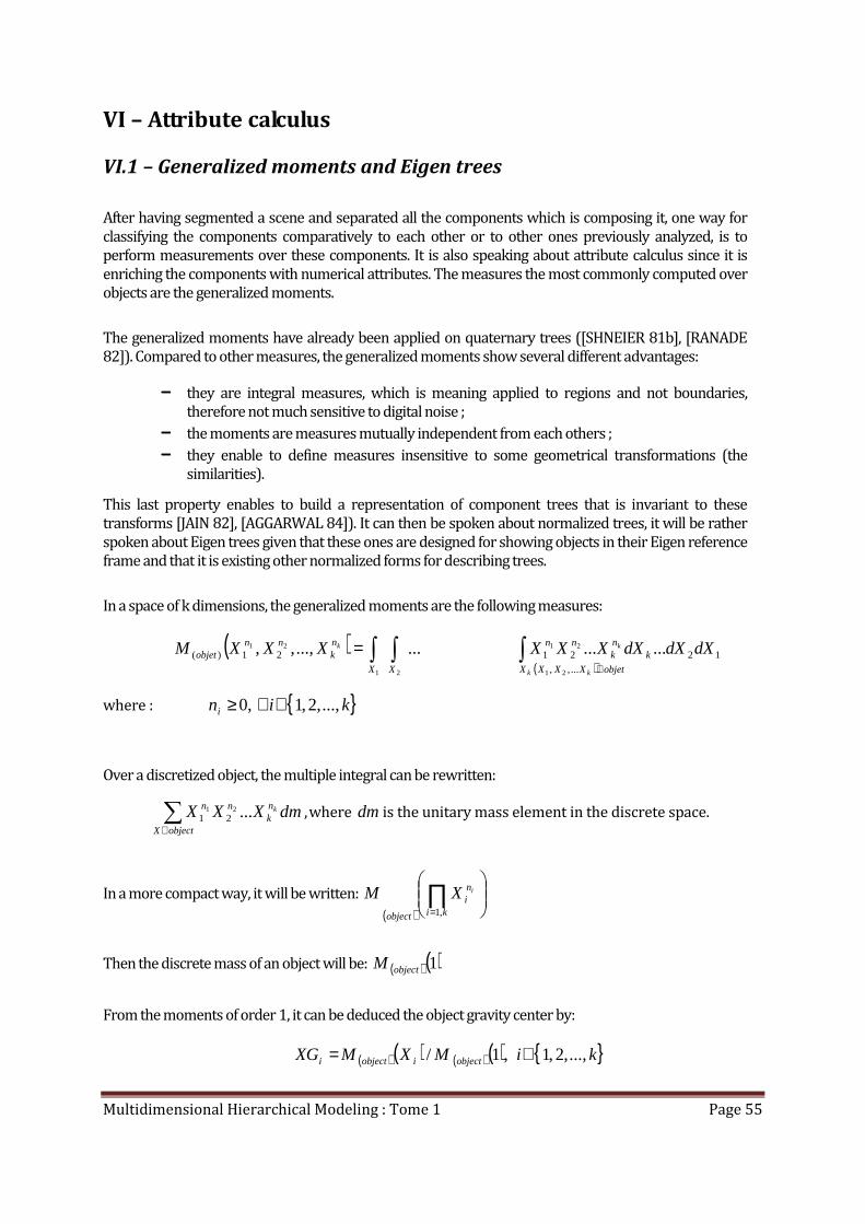
Multidimensional Hierarchical Modeling : Tome 1 Page 55
VI – Attribute calculus
VI.1 – Generalized moments and Eigen trees
After having segmented a scene and separated all the components which is composing it, one way for
classifying the components comparatively to each other or to other ones previously analyzed, is to
perform measurements over these components. It is also speaking about attribute calculus since it is
enriching the components with numerical attributes. The measures the most commonly computed over
objects are the generalized moments.
The generalized moments have already been applied on quaternary trees ([SHNEIER 81b], [RANADE
82]). Compared to other measures, the generalized moments show several different advantages:
−−−− they are integral measures, which is meaning applied to regions and not boundaries,
therefore not much sensitive to digital noise ;
−−−− the moments are measures mutually independent from each others ;
−−−− they enable to define measures insensitive to some geometrical transformations (the
similarities).
This last property enables to build a representation of component trees that is invariant to these
transforms [JAIN 82], [AGGARWAL 84]). It can then be spoken about normalized trees, it will be rather
spoken about Eigen trees given that these ones are designed for showing objects in their Eigen reference
frame and that it is existing other normalized forms for describing trees.
In a space of k dimensions, the generalized moments are the following measures:
( )( )∫∫∫
∈
=objetXXXX
knk
nn
XX
nk
nnobjet
kk
kk dXdXdXXXXXXXM...,,
122121)(
21
21
21
21 ............,,,
where : { }kini ...,,2,1,0 ∈∀≥
Over a discretized object, the multiple integral can be rewritten:
∑∈objectX
nk
nn dmXXX k...2121 , where dm is the unitary mass element in the discrete space.
In a more compact way, it will be written:
( )
∏= ki
ni
object
iXM,1
Then the discrete mass of an object will be: ( ) ( )1objectM
From the moments of order 1, it can be deduced the object gravity center by:
( ) ( ) ( ) ( ) { }kiMXMXG objectiobjecti ...,,2,1,1/ ∈=
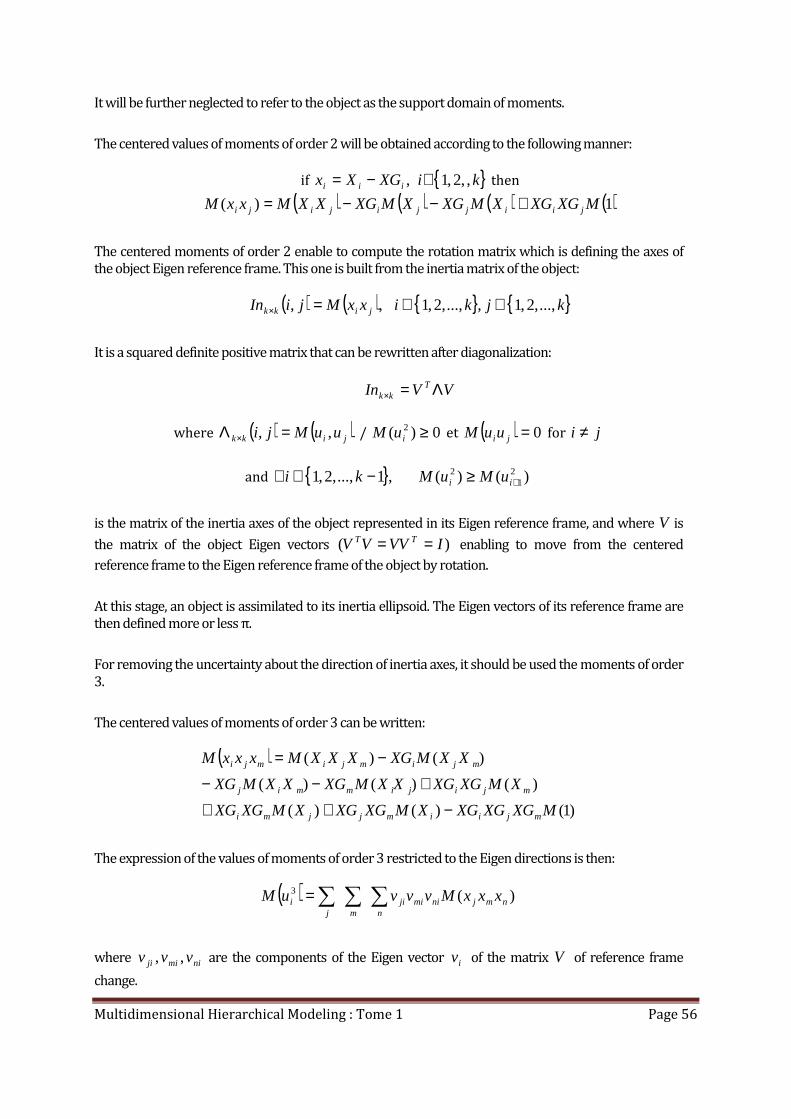
Multidimensional Hierarchical Modeling : Tome 1 Page 56
It will be further neglected to refer to the object as the support domain of moments.
The centered values of moments of order 2 will be obtained according to the following manner:
if { }kiXGXx iii ,,2,1, ∈−= then
( ) ( ) ( ) ( )1)( MXGXGXMXGXMXGXXMxxM jiijjijiji +−−=
The centered moments of order 2 enable to compute the rotation matrix which is defining the axes of
the object Eigen reference frame. This one is built from the inertia matrix of the object:
( ) ( ) { } { }kjkixxMjiIn jikk ...,,2,1,...,,2,1,, ∈∈=×
It is a squared definite positive matrix that can be rewritten after diagonalization:
VVIn Tkk Λ=×
where ( ) ( )jikk uuMji ,, =Λ × / 0)( 2 ≥iuM et ( ) 0=jiuuM for ji ≠
and { } )()(,1...,,2,1 21
2+≥−∈∀ ii uMuMki
is the matrix of the inertia axes of the object represented in its Eigen reference frame, and where V is
the matrix of the object Eigen vectors )( IVVVV TT == enabling to move from the centered
reference frame to the Eigen reference frame of the object by rotation.
At this stage, an object is assimilated to its inertia ellipsoid. The Eigen vectors of its reference frame are
then defined more or less π.
For removing the uncertainty about the direction of inertia axes, it should be used the moments of order
3.
The centered values of moments of order 3 can be written:
( )
)1()()(
)()()(
)()(
MXGXGXGXMXGXGXMXGXG
XMXGXGXXMXGXXMXG
XXMXGXXXMxxxM
mjiimjjmi
mjijimmij
mjimjimji
−++
+−−
−=
The expression of the values of moments of order 3 restricted to the Eigen directions is then:
( ) ∑∑∑=n
nmjnimijimj
i xxxMvvvuM )(3
where nimiji vvv ,, are the components of the Eigen vector iv of the matrix V of reference frame
change.
Multidimensional Hierarchical Modeling : Tome 1 Page 57
The moments of order 3 restricted to the Eigen directions )( 3iuM are the asymmetries of the object
according each of its Eigen axes. They are measuring the object eccentricity along each axis.
The uncertainty of the axis directions is removed by orientating the axes in the direction of the strongest
eccentricity, that is to say in such a meaning where:
{ }kiuM i ...,,2,1,0)( 3 ∈∀≥
That is by replacing iv by its opposite iv− in the matrix V of reference frame change,
when 0)( 3 <iuM .
In such a way, it has been got the matrix of translation, rotation for a displacement of the object tree in its
Eigen reference frame described in homogenous coordinates:
−=
1101
XXGVU T
For obtaining a representation invariant to any scaling, it is only needed to normalize the coordinates
with respect to the main inertia axis:
−=
110
)(
1
121
XXGVuM
U T
This representation might take in account different scaling factors according each axis, but it would not
get any reality concerning rigid body mechanics.
Under1L , all the black nodes observed at any precision in a tree are compact and close sub-sets
of[ [k1,0 .
The binary tree of a set of [ [k1,0 is then a countable compact covering of this set. It is finite when it is
examined at a finite precision. So any measure calculated on the binary tree of a set will be equal to the
sum of measures calculated over each compact sub-set of this covering.
Therefore, it will be possible to compute hierarchically the moments linked to each grey or black nodes
of the tree and to sum them up on the tree traversal return at every non terminal node the contribution
of each terminal node in order to deduce the measures of the object modeled by the tree.
It will be now described a recursive method for the calculus of generalized moments on the blocks
visited during the traversal of a tree representing an object on[ [k1,0 .
To the tree nodes are associated parallelepipeds with edges parallel to the axes:

Multidimensional Hierarchical Modeling : Tome 1 Page 58
[ [ [ [ [ ['''''2
'2
''1
'1 ,,, kk xxxxxx ××× L
That will be assimilated under 1L with:
[ ] [ ] [ ]'''''2
'2
''1
'1 ,,, kk xxxxxx ××× L
And that will be written as:
[ ]∏= ki
ii xx,1
''' ,
These blocks have got for generalized moments:
[ ]( )∏∏
=
++
=
−
+=
∏=
ki
n
i
n
iiki
ni
xx
iii
kiii
xxn
XM,1
1'1''
,1, 1
1
,1
'''
In a binary tree at precision p , a terminal node will get for moment :
[ ]( )11
,1,1, 1
1
,1
++
==
−
+=
∏∏∏
=
iii
kiidig
nig
nid
ki iki
ni
xx
xxn
XM
If the support domain [ ]∏= ki
idig xx,1
, is divided according to jx into sub-sets of same size, it will be got
the following values:
[ ]( )∏∏
≠=
++++
=
+ −+
−
++
=
∏≠= ji
ki
nig
nid
i
njg
n
jdjg
jki
ni
xxxx
x
iij
j
i
jiki
idigjdjg
jg
xxn
xxx
nxM
,1
111
1
,1,2
, 1
1
21
1
,1
Knowing that:
111
011
1
1
2
1
2+−+
+
=++
++
−=−
+∑ jj
j
jj
j
j
njg
mnjd
mjg
n
m
mnn
njg
n
jdjg xxxCxxx
and that:
11
01
1 2)11( ++
=+
+ ==+ ∑ j
j
j
j nn
m
mn
nC
It can be written :
Multidimensional Hierarchical Modeling : Tome 1 Page 59
[ ]
∏∏=
+
≠=
ki
ni
xxxx
x
i
jiki
idigjdjg
jg
xM,1
,2
,,1
[ ]
∏×
−×= ∏∑
=
−
+
+
=+
+
=ki
ni
knj
xx
mjg
j
jn
mn
mn
ij
kiidig
j
j
j xxMxn
nC
,1,1
1
01
1
,1
1
2
Likewise:
[ ]
∏∏=
+
≠=
ki
ni
xxxxx
i
jiki
idigjdjdjg
xM,1
,,2 ,1
[ ]
∏×
−×= ∏∑
=
−
+
+
=+
+
=ki
ni
knj
xx
mjd
j
jn
mn
mn
ij
kiidig
j
j
j xxMxn
nC
,1,1
1
01
1
,1
1
2
For lightening the presentation, it will thereafter only be taken in account of the dividing interval for
displaying the support application domains.
The development of these expressions concerning the generalized moments gives:
At order 0:
( ) [ ]( )( )12
11 ,
2,
jdjgjdjgjg
xxxxx
MM =
+
( ) [ ]( )( )12
11 ,
,2
jdjgjd
jdjgxx
xxx
MM =
+
At order 1:
( ) [ ]( )( )ixxixxx
XMXMjdjgjdjg
jg
,
2, 2
1=
+
( ) [ ]( )( )ixxix
xxXMXM
jdjgjd
jdjg,
,2
2
1=
+
( ) [ ]( )( ) [ ]( )( )14
1
4
1,,
2,
jdjgjdjgjdjgjg
xxjgjxxjxxx
MxXMXM +=
+
( ) [ ]( )( ) [ ]( )( )14
1
4
1,,
,2
jdjgjdjgjd
jdjgxxjdjxxj
xxx
MxXMXM +=
+
And so on until the order 3.
Multidimensional Hierarchical Modeling : Tome 1 Page 60
After having determined the moments of each black k2 -ant of the tree describing the object, the object
moments are then equal to:
( ) ∑ ∏∏∈− ==
=
objectantblack ki
ni
ki
niobject
k
ii XXM2 ,1,1
Computed up to the order 3, the generalized moments provide after centering and normalization:
−−−− at the order 0, the hypervolume of the component,
−−−− at the order 1, its gravity center,
−−−− at the order 2, its inertia axes,
−−−− at the order 3, the signature of its reference frame and its asymmetries according to every
axes.
So the calculus of generalized moments allows to settle a component building invariant to linear positive
transformations that might apply on the component in affine geometry, its Eigen tree.
VI.2 – Pattern recognition
After the centering and the normalization of the moment list of a component, this one is linked to a
vector of measures independent of similarities and symmetries, its attributes:
( ) ( ) ( ) ( )( )331
221 ,,,,, kk uMuMuMuM LL ,
where :
1)( 21 =uM or 0)( 2 >iuM et 0)( 3 >iuM
Therefore the component could be represented by a vector of 12 −k measures.
For implementing a procedure of pattern recognition relying on this representation, it must be built a
learning set made from n experiences:
( ){ } nivf ii ,1,, = ,
where iv is the attribute vector of the i -th experience and if the label attributed to the experience by a
teacher coming from a finite set of possible interpretations (supervised learning).
A procedure of hierarchical classification enables then to classify according to the Hausdorff distance
each new observation expressed using this new form of representation, over the partition of the
interpretations.
In the case of k2 -trees, the learning step consists in building the chromatic tree of dimension 2k-1
modeling the set ( ){ }ii vf , .
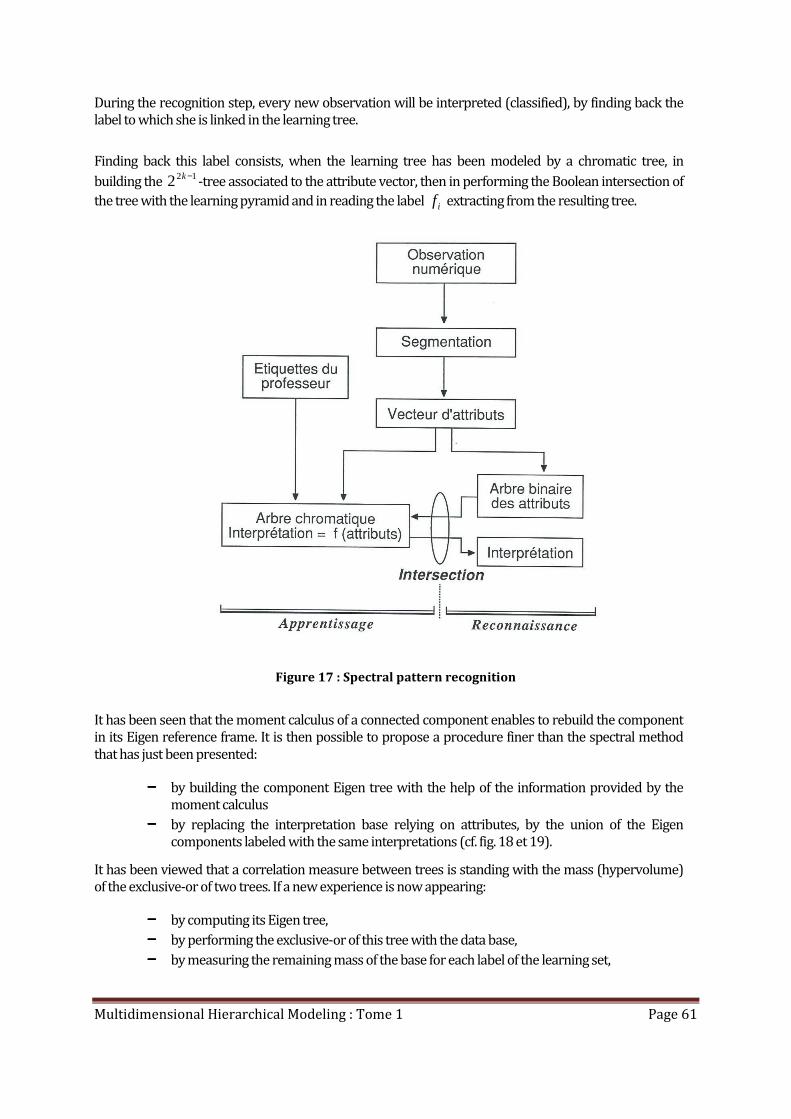
Multidimensional Hierarchical Modeling : Tome 1 Page 61
During the recognition step, every new observation will be interpreted (classified), by finding back the
label to which she is linked in the learning tree.
Finding back this label consists, when the learning tree has been modeled by a chromatic tree, in
building the 122 −k-tree associated to the attribute vector, then in performing the Boolean intersection of
the tree with the learning pyramid and in reading the label if extracting from the resulting tree.
Figure 17 : Spectral pattern recognition
It has been seen that the moment calculus of a connected component enables to rebuild the component
in its Eigen reference frame. It is then possible to propose a procedure finer than the spectral method
that has just been presented:
−−−− by building the component Eigen tree with the help of the information provided by the
moment calculus
−−−− by replacing the interpretation base relying on attributes, by the union of the Eigen
components labeled with the same interpretations (cf. fig. 18 et 19).
It has been viewed that a correlation measure between trees is standing with the mass (hypervolume)
of the exclusive-or of two trees. If a new experience is now appearing:
−−−− by computing its Eigen tree,
−−−− by performing the exclusive-or of this tree with the data base,
−−−− by measuring the remaining mass of the base for each label of the learning set,
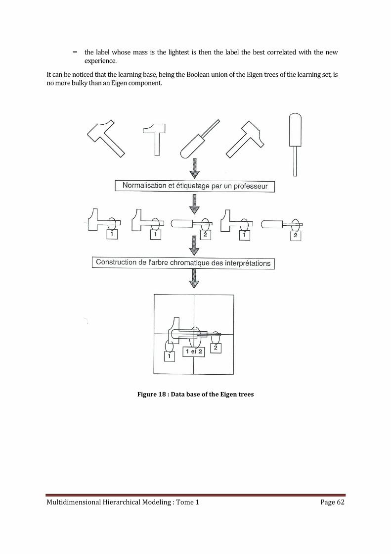
Multidimensional Hierarchical Modeling : Tome 1 Page 62
−−−− the label whose mass is the lightest is then the label the best correlated with the new
experience.
It can be noticed that the learning base, being the Boolean union of the Eigen trees of the learning set, is
no more bulky than an Eigen component.
Figure 18 : Data base of the Eigen trees
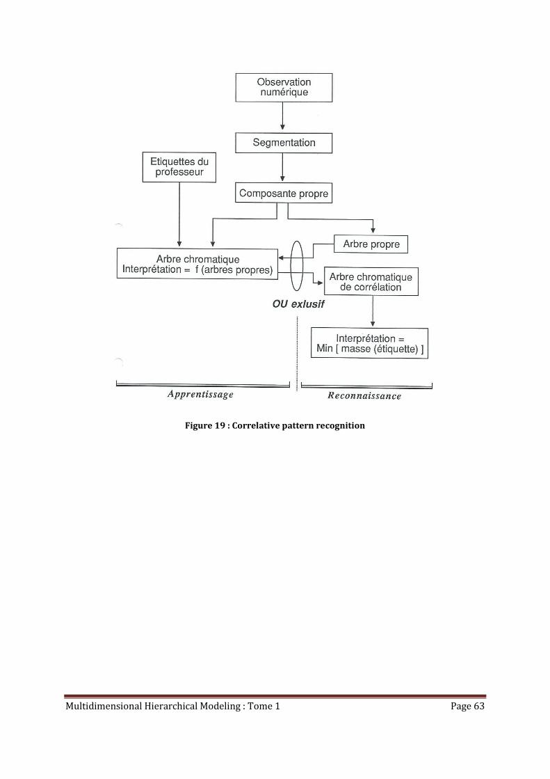
Multidimensional Hierarchical Modeling : Tome 1 Page 63
Figure 19 : Correlative pattern recognition

Multidimensional Hierarchical Modeling : Tome 1 Page 64
Multidimensional Hierarchical Modeling : Tome 1 Page 65
Conclusion
This presentation about k2 -trees modeled by binary trees has shown that the results obtained by the
past on quaternary and octernary trees can be extended to spaces of any dimension.
The proposed tree building method is compatible with disorderly and overcrowded data streams.
Its inductive limit extension enables to avoid any previous normalization of the data, while insuring the
comparability of trees generated independently the ones from the others.
The computation of the homographic transform of a k2 -tree has clarified the properties of convex
analysis needed for performing such a transformation, used by some authors in spaces of two or three
dimensions.
As it has been widely pointed out, the calculus of attributes based on the generalized moments enables
to:
−−−− localize in position and in orientation, an object in its observation space ;
−−−− deduce a vector of measures invariant to similarities ;
−−−− propose for each object a description independent from its observation space, its Eigen
tree.
It has been described the principles of segmentation relying on two distances 1d et ∞d induced by the
structure of mesh associated to k2 -trees.
These principles enable to define the notion of object as a connected component. According to this
approach, they enable to implement perception procedures of objects without any recovering in affine
geometry.
Two methods of unsupervised pattern recognition have been described.
A third unsupervised one can be designed in introducing a supplementary segmentation stage applied
in the attribute space in the case of the spectral pattern recognition: the membership class is the
connected component reached after the learning phase.
These techniques mix several different approaches commonly met in statistical data analysis:
−−−− Bayesian, where the tree of a connected component modeled a probability distribution ;
−−−− by partitioning while proposing two segmentation methods ;
−−−− by hierarchical classification knowing that the representation model is driven by an
ultrametric distance, the Hausdorff distance;
−−−− factorial analysis, by the means of generalized moments.
In the framework of the mid-term study which has enabled to perform these works, some other aspects
of the question have been also studied:

Multidimensional Hierarchical Modeling : Tome 1 Page 66
−−−− the computation of the convex hull of a multidimensional object (checking the linear
separation of classes) ;
−−−− the insertion, the extraction of manifolds parallel to the reference frame(parallel slices) ;
−−−− the homotopic transformations (erosion, dilation, median filtering) ;
−−−− the calculus of the integral equation system of a continuous manifold by approximation
with variable order polynomials and the building of the atlas of maps of a piecewise
continuous manifold;
−−−− the search of Hamiltonian paths on data sets (Peano-Hilbert scanning) ;
−−−− the recognition of patterns partially hidden in projective geometry by building dual trees ;
−−−− the analysis of parallel architecture computers agreeing with this kind of algorithmic
(mainly parallel architectures based on multiple interconnection networks).
Multidimensional Hierarchical Modeling : Tome 1 Page 67
Bibliography
[AHO 74] A.V. AHO, J.E. HOPCROFT, J.D. ULLMAN: The Design and Analysis of
Computer Algorithms; Addison-Wesley Publishing Company, 1974.
[ABEL 84a] D.J. ABEL: A B+Tree Structure for Large Quadtrees ; CGIP 27, 19,31, 1984.
[ABEL 84b] D.J. ABEL: Comments On "Detection of Connectivity for Regions
Represented by Linear Quadtrees"; Comp. & Maths. WITH Appls., Vol. 10,
N° 2, 1984.
[ABEL 85] D.M. MARK, D.J. ABEL: Linear Quadtrees from Vector Representations of
Polygons; IEEE Tr. on PAMI, Vol. 7, N° 3, May 1985.
[AGGARWAL 84] C.H. CHIEN, J.K. AGGARWAL: A Normalized Quadtree Representation;
CGIP 26, 331-346, 1984.
[AHUJA 83] N. AHUJA: On Approaches to Polygonal Decomposition for Hierarchical
Image Representation; CGIP 24, 200-214, 1983.
[AHUJA 84] N. AHUJA, C. NASH: Octree Representations of Moving Objects; CGIP 26,
206-216, 1984.
[ALEXANDRIDIS 78] N. ALEXANDRIDIS, A. KLINGER: Picture Decomposition, Tree Data-
Structures, and Identifying Directional Symmetries as Node
Combinations; CGIP 8, 43-77, 1978.
[ALEXANDRIDIS 84] F.W. BURTON, J.G. KOLLIAS, N.A. ALEXANDRIDIS: An Implementation of the Exponential Pyramid Data Structure with Application to Determination of Symmetries in Pictures; CGIP 25, 218-225, 1984.
[ALEXANDRONOV 84] V.V. ALEXANDRONOV, N.D. GORSKY, S.N. MYSKO: Recursive Pyramids and Their Use for Image Coding; Pattern Recognition Letters 2, 301-310, 1984.
[BALLARD 82] D.H. BALLARD, C.M. BROWN: Computer vision; Prentice Hall, 1982.
[BENTLEY 75] J.L. BENTLEY: Multidimensional Binary Search Trees Used for Associative
Searching; CACM, Vol. 18, N° 9, September 1975.
[BENTLEY 80] J.L. BENTLEY: Multidimensional Divide-and-Conquer; CACM, Vol. 23, N° 4,
April 1984.
[BURTON 85] F.W. BURTON, V.J. KOLLIAS, J.G. KOLLIAS: Expected and Worst Case
Storage Requirements for Quadtrees; Patter Recognition Letters 3, 131-
135, 1985.
[CHAUDHURI 85] B.B. CHAUDHURI: Applications of Quadtree, Octree, and Binary Tree Decomposition Techniques to Shape Analysis and Pattern Recognition; IEEE Tr. on PAMI, Vol. 7, N° 6, November 1985.
[CYGANSKI 85] D. CYGANSKI, J.A. ORR: Application of Tensor Theory to Object Recognition and Orientation Determination; IEEE Tr. on PAMI, Vol. 7, N° 6, November 1985.
Multidimensional Hierarchical Modeling : Tome 1 Page 68
[DYER 80] C.R. DYER: Computing the Euler Number of an Image from its Quadtree; CGIP 13, 270-276, 1980.
[DYER 82] C.R. DYER: The Space Efficiency of Quadtrees; CGIP 19, 335-348, 1982.
[FAVERJON 84] B. FAVERJON: Obstacle Avoidance Using an Octree in the Configuration Space
of a Manipulator; IEEE 1984, 504-512.
[GARGANTINI 82a] I. GARGANTINI: An Effective Way to Represent Quadtrees; CACM, Vol. 25, N° 12, December 1982.
[GARGATNTINI 82b] I. GARGANTINI: Linear Octrees for Fast Processing of Three-Dimensional Objects; CGIP 20, 365-374, 1982.
[GARGANTINI 82c] I. GARGANTINI: Detection of Connectivity for Regions Represented by Linear Quadtrees; Comp. and Math. with Appls, Vol. 8, N° 4, 1982.
[GARGANTINI 83a] I. GARGANTINI: Translation, Rotation and Superposition of Linear Quadtrees; Int. J. Man-Machine Studies 18, 253-263, 1983.
[GARGANTINI 83b] I. GARGANTINI, G. LAM: An Approximation to the 3D Border; Proc. Soc. Photo. Inst. Eng. SPIE, Genève, 98-103, 1983.
[GARGANTINI 83c] I. GARGANTINI: The Use of Linear Quadtrees in A Numerical Problem; SIAM J. Numer. Anal, Vol. 20, N° 6, December 1983.
[GARGANTINI 84a] H.H. ATKINSON, I. GARGANTINI, M.V.S. RAMANATH: Determination of the 3D Border by Repeated Elimination of Internal Surfaces; Computing 32, 279-295, 1984.
[GARGANTINI 84b] I. GARGANTINI, H.H. ATKINSON: Linear Quadtrees: A Blocking Technique
For Contour Filling; Pattern Recognition, Vol. 17, N° 3, 1984.
[GARGANTINI 86a] H.H. ATKINSON, I. GARGANTINI, T.R.S. WALSH: Filling by Quadrants for Octants; CGIP 33, 138-155, 1985.
[GARGANTINI 86b] I. GARGANTINI, T.R. WALSH, O.L. WU: Viewing Transformations of Voxel-Based Objects via Octrees ; IEEE CG & A., October 1986.
[GOSHTASBY 85] A. GOSHTASBY: Template Matching in Rotated Images; IEEE Tr. on PAMI, Vol. 7, N° 3, May 1985.
[HAMMING 50] R.W. HAMMING: Error Detecting and Error Correcting Codes; Bell System Tech. L, 29, 147-160, 1950.
[HERBERT 85] F. HERBERT: Solid Modeling for Architectural Design using Octpaths; Computer and Graphics, Vol. 9, N° 2, 1985.
[HONG 85] T.-H. HONG, M. SHNEIER: Describing a Robot's Workspace Using a Sequence of Views from a Moving Camera; IEEE Tr. on PAMI, Vol. 7 , N° 6, November 1985.
[HOROWITZ 76] S.L. HOROWITZ, T. PAVLIDIS: Picture Segmentation by a Tree Traversal Algorithm; Journal of the ACM, Vol. 23, N° 2, April 1976.
[HUNTER 79a] G.M. HUNTER, K. STEIGLITZ: Operations on Images Using Quadtrees; IEEE Tr. PAMI, Vol. 1, N° 2, April 1979.
Multidimensional Hierarchical Modeling : Tome 1 Page 69
[HUNTER 79b] G.M. HUNTER, K. STEIGLITZ: Linear Transformation of Pictures Represented by Quadtree; CGIP, N° 10, 289 - 296, 1979.
[JACKINS 80] C.L. JACKINS, S.L. TANIMOTO: Oct-Trees and Their Use in Representing Three-Dimensional Objects; CGIP 14, 249-270, 1980.
[JACKINS 83] C.L. JACKINS, S.L. TANIMOTO: Quad-Trees, Oct-Trees, and K-Trees: A Generalized Approach to Recursive Decomposition of Euclidean Space; IEEE Tr. on PAMI, Vol. 5, September 1983.
[JAIN 82] M. LI, W.I. GROSKY, R. JAIN: Normalized Quadtrees with Respect to Translation; CGIP 20, 72-81, 1982.
[JONES 84] L.P. JONES, S.S. IYENGAR: Space and Time Efficient Virtual Quadtrees; IEEE Tr. on PAMI, Vol. 6, N° 2, March 1984.
[KLINGER 76] A. KLINGER, C.R. DYER: Experiments on Picture Representation Using Regular Decomposition; CGIP 5, 68-105, 1976.
[KLINGER 79] A. KLINGER, M.L. RHODES: Organization and Access of Image Data by Areas; IEEE Tr. PAMI, Vol. 1 N° 1, January 1979.
[KNUTH 73] D.E. KNUTH: The Art of Computer Programming: Fundamental Algorithms, Vol. 1, Addison-Wesley, 1973.
[KUNT 87] M. KUNT, M. BENARD, R. LEONARDI: Recent Results in High Compression Image Coding; IEEE Tr. on CAS, Vol. 34, N° 11, November 1987.
[LEE 86] C.-H. LEE: Recursive Region Splitting at Hierarchical Scope of Views; CGIP 33, 237-258, 1986.
[LIBERA 86] F.D. LIBERA, F. GOSEN: Using B-trees to Solve Geographic Range Queries; The Computer Journal, Vol. 29, N° 2, 1986.
[LOZANO-PEREZ 85] R.A. BROOKS, T. LOZANO-PEREZ: A Subdivision Algorithm in Configuration Space for Find path with Rotation; IEEE Tr. on SMC, Vol. 15, N° 2, March/April 1985.
[MEAGHER 80] Octree encoding: A new technique for the representation and display of arbitrary 3-D objects by computer; IPL - TR - 80-111, Image Processing Lab., Electrical and Systems Engineering Dept., Rensselaer Polytechnic Institute, October 1980.
[MEAGHER 82a] D. MEAGHER: Geometric Modeling Using Octree Encoding; CGIP, N° 19, 129-147, 1982.
[MEAGHER 82b] D. MEAGHER: Octree Generation, Analysis and Manipulation; IPL - TR - 82-027, Image Processing Lab., Electrical and Systems Engineering Dept., Rensselaer Polytechnic Institute, April 1982.
[NEWMAN 73] N.M. NEWMAN, R.F. SPROULL: Principles of Interactive Computer Graphics; New York, Mc Graw-Hill, 1973.
[OLIVER 83a] M.A. OLIVER, N.E. WISEMAN: Operations on Quadtree Encoded Images; The Computer Journal, Vol. 26, N° 1, 1983.
Multidimensional Hierarchical Modeling : Tome 1 Page 70
[OLIVER 83b] M.A. OLIVER, N.E. WISEMAN: Operations on Quadtree Leaves and Related Images; The Computer Journal, Vol. 26, N° 4, 1983.
[PAVEL 85] Y. COHEN, M.S. LANDY, M. PAVEL: Hierarchical Coding of Binary Images; IEEE Tr. on PAMI, Vol. 7, N° 3, May 1985.
[PAVLIDIS 77] T. PAVLIDIS: Structural Pattern Recognition; Springer-Verlag, 1977.
[PAVLIDIS 78] T. PAVLIDIS: A Review of Algorithms for Shape Analysis; CGIP 7, 243-258, 1978.
[PAVLIDIS 82] T. PAVLIDIS: Algorithms for Graphics and Image Processing; Computer Science Press, 1982.
[PREPARATA 84] D.T. LEE, F.P. PREPARATA: A Computational Geometry; IEEE Tr. on Computers, Vol. 33, N° 12, December 1984.
[PREPARATA 85] F.P. PREPARATA, M.I. SHAMOS: Computational Geometry: An Intro-duction; Springer-Verlag, 1985.
[RANADE 81a] S. RANADE: Use of Quadtrees for Edge Enhancement; IEEE Tr. SMC, Vol. 11, N° 5, May 1981.
[RANADE 81b] S. RANADE, M. SHNEIER: Using Quadtrees to Smooth Images; IEEE Tr. SMC, Vol. 11, N° 5, MAY 1981.
[RANADE 82] S. RANADE, A. ROSENFELD, H. SAMET: Shape Approximation Using Quadtrees; Pattern Recognition, Vol. 15, N° 1, 1982.
[ROSENFELD 70] A. ROSENFELD: Connectivity in Digital Pictures; Journal of the ACM, Vol. 17, N° 1, January 1970.
[ROSENFELD 82a] A. ROSENFELD, A.C. KAK: Digital Picture Processing; Academic Press 1982.
[ROSENFELD 82b] A.Y. WU, T.H. HONG, A. ROSENFELD: Threshold Selection Using Quadtrees; IEEE Tr. PAMI, Vol. 4, N° 1, January 1982.
[ROSENFELD 83b] A. ROSENFELD: Quadtrees and Pyramids Hierarchical Representation of Images; in Pictorial Data Analysis, ED: R.M. HARALICK; NATO ASI Series, Computer and Systems Sciences N° 4, 1983.
[ROSENFELD 84a] A. ROSENFELD: Image Analysis: Problems, Progress and Prospects; Pattern Recognition, Vol. 17, N° 1, 1984.
[ROSENFELD 84b] Ed: A. ROSENFELD: Multiresolution Image Processing and Analysis; Springer-Verlag, 1984.
[SAMET 79] H. SAMET: Region Representation: Raster-to-Quadtree Conversion; Computer Science TR-766, University of Maryland, College Park, Maryland, May 1980.
[SAMET 80a] H. SAMET: Region Representation: Boundary Codes from Quadtrees; CGIP 13, 88-93, 1980.
[SAMET 80b] H. SAMET: Region Representation: Quadtrees from Boundary Codes; CACM, Vol. 23, N° 3, March 1980.
Multidimensional Hierarchical Modeling : Tome 1 Page 71
[SAMET 80c] C.R. DYER, A. ROSENFELD, H. SAMET: Region Representation: Boundary Codes from Quadtrees; CACM, Vol. 23, N° 3, March 1980.
[SAMET 81a] H. SAMET: Connected Component Labelling Using Quadtrees; J. ACM 28, 487-501, 1981.
[SAMET 81b] H. SAMET: Computing Perimeters of Regions in Images Represented by Quadtree; IEEE Tr. PAMI, Vol. 3, N° 6, November 1981.
[SAMET 82a] H. SAMET: Neighbor Finding Techniques for Images Represented by Quadtrees; CGIP 18, 37-57, 1982.
[SAMET 82b] H. SAMET: Distance Transform for Images Represented by Quadtrees; IEEE Tr. PAMI, Vol. 4, N° 3, May 1982.
[SAMET 83] H. SAMET: A Quadtree Medial Axis Transform; CACM, Vol. 26, N° 9, September 1983.
[SAMET 84a] H. SAMET: Algorithms for the Conversion of Quadtrees to Rasters; CGIP 26, 1-16, 1984.
[SAMET 84b] H. SAMET, R.E. WEBBER: On Encoding Boundaries with to Quadtrees; IEEE Tr. on PAMI, Vol. 6, N° 3, May 1984.
[SAMET 84c] H. SAMET, A. ROSENFELD, C.A. SHAFFER, R.E. WEBBER: A Geographic Information System Using Quadtrees; Pattern Recognition, Vol. 17, N° 6, 1984.
[SAMET 84d] H. SAMET: The Quadtree and Related Hierarchical Data Structures; Computing Surveys, Vol. 16, N° 2, June 1984.
[SAMET 84e] H. SAMET, M. TAMMINEN: Experiences with New Image Component Algorithms; EUROGRAPHICS 84, Elsevier Science Publishers B.V., 239-249, 1984.
[SAMET 85a] H. SAMET: A Top-Down Quadtree Traversal Algorithm; IEEE Tr. On PAMI, Vol. 7, N° 1, January 1985.
[SAMET 85b] H. SAMET, M. TAMMINEN: Computing Geometric Properties of Images Represented by Linear Quadtrees; IEEE Tr. on PAMI, Vol. 7, N° 2, March 1985.
[SAMET 85c] H. SAMET: Reconstruction of Quadtrees from Quadtree Medial Axis Transforms; CGIP 29, 311-328, 1985.
[SAMET 85d] H. SAMET: Data Structures for Quadtree Approximation and Compression; CACM, Vol. 23, N° 9, September 1985.
[SAMET 85e] H. SAMET, C.A. SHAFFER: A Model for the Analysis of Neighbor Finding in Pointer-Based Quadtrees; IEEE Tr. on PAMI, Vol. 7, N° 6, November 1985.
[SHEPARD 85a] M.S. SHEPARD, N.A.B. YEHIA, G.S. BURD, T.J. WEIDNER: Computational Strategies for Non linear and Fracture Mechanics problems: Automatic Crack Propagation Tracking; Computers & Structures, Vol. 20, N° 1, 1985.
Multidimensional Hierarchical Modeling : Tome 1 Page 72
[SHEPARD 85b] M.A. YERRY, M.S. SHEPARD: Trends in Engineering Software and Hardware: Automatic Mesh Generation for Three-Dimensional Solids ; Computers & Structures, Vol. 20, N° 1, 1985.
[SHNEIER 81a] M. SHNEIER: Path-Length Distances for Quadtrees; Information Sciences 23, 49-67, 1981.
[SHNEIER 81b] M. SHNEIER: Calculations of Geometric Properties Using Quadtrees; CGIP 16, 296-302, 1981.
[SIMON 80] J.C. SIMON, J. QUINQUETON: On the Use of a PEANO Scanning in Image Processing; in Issues in Digital Image Processing, Ed.: R.M. HARALICK, J.C. SIMON; NATO ASI SERIES, APPLIED SCIENCE N° 34, 1980.
[SRIHARI 81] S.N. SRIHARI: Representation of Three-Dimensional Digital Images; Computing Surveys, Vol. 13, N° 4, December 1981.
[SRIHARI 82] S.N. SRIHARI: Hierarchical Data Structures and Progressive Refinement of 3-D Images; 1982 IEEE?
[SRIHARI 84] D.M. HARDAS, S.N. SRIHARI: Progressive Refinement of 3-D Images Using Coded Binary Trees: Algorithms and Architecture; IEEE Tr. on PAMI, Vol. 6, N° 6, November 1984.
[SUK 83] M. SUK, N.M. CHUNG: A New Image Segmentation Technique Based on Partition Mode Test; Pattern Recognition, Vol. 16, N° 5, 1983.
[SUTHERLAND 74b] I.E. SUTHERLAND, R.F. SPROULL, R.A. SCHUMACKER: A Characterization of Ten Hidden-Surface Algorithms; ACM Computing Surveys, Vol. 6, N° 1, 1974.
[TAMMINEN 84a] M. TAMMINEN: Comment on Quad-and-Octrees; CACM, Vol. 27, N° 3, March 1984.
[TAMURA 84] H. TAMURA, N. YOKOYA: Image Database Systems: a Survey; Pattern Recognition, Vol. 17, N° 17, 1984.
[TANIMOTO 75] S. TANIMOTO, T. PAVLIDIS: A Hierarchical Data Structure for Picture Processing; CGIP 4, 104_119, 1975.
[TANIMOTO 80] S. TANIMOTO, A. KLINGER (Eds): Structured Computer Vision: Machine Perception through Hierarchical Computation; Academic Press, NY, 1980.
[TARJAN 84] D. HAREL, R.E. TARJAN: Fast Algorithms for Finding Nearest Common Ancestors; SIAM J. Comput., Vol. 13, N° 2, May 1984.
[VAN LIEROP 86] M.L.P. VAN LIEROP: Geometric Transformations on Picture Represented by Leafcodes; CGIP 33, 81-98, 1986.
[WARNOCK 69] J.E. WARNOCK: A Hidden-Surface Algorithm for Computer Generated Half-Tone Pictures, TR-4-15, University of UTAH, 1969.
[WOODWARK 82] J.R WOODWARK: The Explicit Quadtree as a Structure for Computer Graphics; The Computer Journal, Vol. 25, N° 2, 1982.
[WOODWARK 84] J.R. WOODWARK: Compressed Quadtrees; The Computer Journal, Vol. 27, N° 3, 1984.

Multidimensional Hierarchical Modeling : Tome 1 Page 73
[YAU 81] M.M. YAU, S.N. SRIHARI: Digital Convex Hulls from Hierarchical Data Structures; CMCCS 81/ACCMO 81.
[YAU 83] M.M. YAU, S.N. SRIHARI: A Hierarchical Data Structure for Multidimensional Digital Images; CACM, Vol. 26, N° 7, July 1983.
[YAU 84] M.M. YAU: Generating Quadtrees of Cross Sections from Octrees; CGIP 27, 211-238, 1984.
[YERRI 83] M.A. YERRI, M.S. SHEPARD: A Modified Quadtree Approach to Finite Element Mesh Generation; IEEE CG & A, January/February 1983.
[ZAHN 71] C.T. ZAHN: Graph-Theoretical Methods for Detecting and Describing Gestalt Clusters; IEEE Tr. on Computers, Vol. 20, N° 1, January 1971.
[ZUCKER 76] S.W. ZUCKER: Region Growing Childhood and Adolescence; CGIP 5, 382-399, 1976.

Multidimensional Hierarchical Modeling : Tome 1 Page 74
Multidimensional Hierarchical Modeling : Tome 1 Page 75
Glossary
adjacency : direct link between two points of a graph, proximity relation in discrete
geometry, the most often deducted from the distance used on the space of interest
(cf. distance, neighborhood, connectivity).
aggregation : method in statistical analysis that enables to gather data sets or to compute
measures over these sets (aggregating indicators used for instance in the building of
dashboards).
Boolean algebra : set algebra, all the operations that can be the result of a combination of
elementary set operations (assertion, negative, union, intersection, exclusion,
difference).
Borel algebra : set made from all the parts of a space that are enclosed for the algebraic
operations that can be applied on – if the number of applied operations is countable
then it is a sigma-algebra. The sigma-algebras are at the foundation of the theories of
measure and probabilities– in the present case, they are semi-open intervals coming
from the regular decomposition of the unitary space down to a finite integer precision
for a Borel algebra and a sigma-algebra when the precision is approaching the
infinite.
relational algebra : all the operations that can apply on a data set and which made from the
combination of a finite number of elementary relational operations (union,
intersection, jointure, Cartesian product,...).
algorithm : computing procedure applying the one after the other a finite number of simple
computing rules enabling to perform a complex function – it can be distinguished
sequential algorithms from parallel ones where the order followed for processing
operations and data is not the same.
altimetry : technique for measuring altitudes, by extension the set of altitudes regularly
sampled on a planar cartographic support.
analysis : decomposition of a whole into its parts (cf. synthesis)
factor analysis : statistical data analysis technique based on the search and the visualization
of data according to their first factors (main inertial axes of the data cloud).
image analysis : all the image decomposition techniques into elementary subsets, that are
functional values regularly sampled on planar supports.
linear analysis : mathematical analysis technique focusing on the decomposition of
functions at first differential order in multidimensional spaces and on their handling
using matrix algebra, enabling for instance to directly solve inverse systems.
spatial analysis : part of statistical analysis which is dealing with random systems evolving
within space.
Multidimensional Hierarchical Modeling : Tome 1 Page 76
statistical analysis : analysis of random systems containing a large number of elements, in
which it is tried to distinguish exogenous factors from endogenous ones with the help
of several observations on a same event.
structural analysis : part of systems analysis dealing with the decomposition of systems into
subsystems and the study of exchanges that they may have between them using
exchanges matrices or interconnection graphs.
time-series analysis : part of statistical analysis which is dealing with random systems
evolving with time.
approximation : numerical method enabling to reproduce a data set with a given error -
usually its upper bound is controlled, and it provides a mathematical model which is
fitting to an initial data set.
archiving : gather, classify and preserve pieces of information.
first level archiving : archiving of new pieces of information in a raw format without
applying any processing
second level archiving : archiving of old or of compressed pieces of information.
attitude : orientation information about an object in its frame of reference : in the plane,
angle of the main inertia axis with the abscissa axis of the reference frame; in the
space, matrix of object Euler angles in its reference frame.
attributes : measures computed on the whole set of data defining an object (they are also
called characteristics) ; they enable to apply statistical pattern recognition
techniques for identifying objects.
attributes in differential geometry: measures applying on surface data (in other words
functions evolving according to a planar support), as the surface mean, the tangent
plane, the curvature tensor.
attributes in discrete geometry : measures applying on volume data (in other words
functions evolving according to a tridimensional support), as the generalized
moments, the inclosing rectangle, the form factor.
attributes in statistical analysis : measures applying on object populations from which can
be inferred a mean vector, a variance-covariance matrix, etc...
authentication : pattern recognition process where it is not tried to identify a shape, but
only to confirm that it is the right one that it is expected to find (the plausibility of a
proposed label for an observed shape is only checked).
Eigen axes : or also axes of inertia, they enable to assimilate an object with its inertia
ellipsoid and provide information about the attitude of an object around its gravity
center; they are deduced from its generalized moments and enable to define the
Eigen frame of reference of an object.

Multidimensional Hierarchical Modeling : Tome 1 Page 77
median axes : set of points that are at equal distance from the borders of an object ; it is a
topological description that can vary according to the used distance, also named the
skeleton of an object.
principal axes : they are the axes that are gathering the main part of inertia among all the
Eigen axes, in statistical data analysis, they enable to reduce the observing space
down to a sub-space of lower dimension and to observe data with losing only a small
part of the information (descriptive analysis).
boundary : set of points belonging to a connected component that are both connected to the
inside and the outside of the component.
cataloging : identifying, indexing and summarizing information.
characteristics : attributes.
classes : sub-sets sharing the same property.
classification : defining classes.
computer architecture classification : Flynn has settled a computer architecture
classification relying on the degree of multiplicity of instruction and data streams
(SISD, MISD, SIMD MIMD), to which can be linked a programming model named
SPMD that can apply on the two different situations of massive parallelism (SIMD,
SPMD over MIMD architecture).
hierarchical classification : classification methods leading to the building of nested
partitions, usually modeled by tree-like structures where parts can be compared
between them using an ultrametric distance.
partitioning-based classification : classification methods based on the building of a
partition over a data set.
supervised classification : to set up classes where the way how to classify is shown by a
teacher, this one labels a learning set with the labels of the expected classes.
thematic classification : from multispectral image analysis in remote sensing, classification
of luminescence vectors of images points, so as to attempt and to recover the
physical nature of elements covering the ground (snow, water, fields, forests, urban
areas,...).
unsupervised classification: to set up classes where the way how to classify is straightly
computed using a classification method without the help of a teacher for labeling a
learning set.
compactness : for a shape, it is a state which is similar to some neighborhoods or to a small
union of neighborhoods belonging to the topology of the descriptive space – in
planar image analysis, the compactness of an object can be measured with the help of
form factor which is the ratio of the object surface on the square of its perimeter : the
closer to one it is, the more compact the form is.

Multidimensional Hierarchical Modeling : Tome 1 Page 78
connected component : subset made from connected points(equivalence class according to a
relation of connectivity or adjacency).
homogeneous component : subset of data of same kind.
compression : action enabling to reduce the size of an information set (analysis) ; the original
set is retrieved by decompression (synthesis).
lossless compression : compression method for which it is sure to retrieve the whole
original information, it is usually similar to perform a format conversion.
lossy compression : compression method for which it is not sure that at decompression time
original information can be retrieved without any loss.
asynchronous computer : parallel architecture computer where each processor has at its
disposal a control unit applying on its own instruction stream, enabling to perform
different programs over the data set to be processed.
synchronous computer : parallel architecture computer where all the processors share a
same control unit applying on the instruction stream, implying the performance of a
single program simultaneously on all over the data set to be processed.
high-performance computing : performance of algorithms where numerical computing is
prevailing (first instance, solving high-dimensional differential equation systems).
parallel computing : performance of algorithms on specific architecture computers, favoring
parallel processing on similar computing units enabling to decrease their processing
time.
vector computing : performance of algorithms on specific architecture computers, favoring
the parallel processing of given arithmetic operations for data appearing under the
form of numerical vectors.
connectivity : link or straight relation between two points in a set ; usually proximity relation
in a metric space, neighborhood relation in a discrete space.
contour : boundary of an object in the plane ; it has the property to be visited only once and
using only one way (border following).
format conversion : operation enabling to convert a data set from one data format to another
one.
thematic conversion : during or after a thematic classification, operation enabling to convert
a multispectral image into a thematic image whose pseudo-colors depict the theme
linked to the luminescence vectors identified during the classification step.
connectivity degree : number of elements to which an element can be related.
expansion degree : rank up to which a function can be approximated using a limited
expansion (degree 0, constant function - degree 1, linear - degree 2, quadric - degree
3, cubic).

Multidimensional Hierarchical Modeling : Tome 1 Page 79
singularity degree : expansion degree for which a function cannot be approximated in a
given location of its support – its functional or its differential tensor up to this degree
is not locally continuous.
intrinsic dimension : roughly, dimension of the space in which an object can be mapped
using a continuous transform in such a way that it would recover a main part of this
space; so the intrinsic dimension of a point is zero, the value for a curve is one, and
two for a surface – using piecewise linear fitting, these elements correspond to points,
lines and surfaces in cartography.
distance : measure enabling to value the proximity of two points (metric) or two point sets
(ultrametric), print a particular topology over the corresponding space and rely on a
specific mesh, when this space is discretized.
metric distance : usually on the dk distances(k-th root of the sum of the p-th power of the
absolute value of the coordinates difference), three from them are the most useful, d1
and d∞ that can be discretized on regularly sampled meshes according to each
dimension of the space and d2 that can be discretized in the plane using a hexagonal
mesh.
ultrametric distance : a main focus is applied on Haussdorf or Hamming distances, which are
compliant with regular meshes built using d1 and d∞, and generate over these spaces
rougher topologies, but for which a partition can be hierarchically handled (for
instance by using trees of degree 2k).
division : resolution principle used by the algorithms that are following the "divide and
conquer" paradigm which consists in decomposing a problem into sub-problems
when they cannot be straightly solved; it prints out a hierarchical structure over the
processed data for solving the corresponding problem (a quick sort, a fast Fourier
transform or the building of a convex hull are following this method in order to
provide algorithms optimal in computing time).
epigraph : half-space above a curve or a surface.
expansion : operation enabling to extend a discrete data set so as to produce a continuous
covering of the support space – this operation includes an hypothesis concerning the
data distribution – used at degree 0 for building a continuous covering of a labeled
space during a statistical learning.
convolutional filtering : numerical filtering of a signal based on the use of a convolution
operator, which degree enables to perform or an integration operation, either a
derivative operation on the numerical data.
topological filtering : or morphological filtering, based on the recursive use of two basic
transform, erosion and dilatation – it applies on binary data (support space) or on
multi-valued data (functional space).
forest : collection of un-connected graphs, the more often trees representing connected
components of the space.
Multidimensional Hierarchical Modeling : Tome 1 Page 80
polygon filling : format conversion enabling to transform a vectorized representation model
into a cellular representation model.
garbage-collector : process enabling to reorganize the free space of a variable-legnth
memory allocation system.
analytic geometry : specific field of geometry which is focused on the handling of geometric
shapes using analytic expansions, that is to decompose forms into primitives
(approximation using expansions in series for representing curves or surfaces).
computational geometry : specific field of geometry which is dealing with algorithms
enabling to extract and to transform geometrical structures registered in numerical
data sets.
constructive geometry : synthesis of geometrical objects by using algebraic combinations
(with the help of Boolean operations completed with some affine transformations) of
complex geometric shapes.
differential geometry : extension of analytic geometry where the coefficients implied in series
expansion are interpreted as local differential operators and with whose help it is
possible to extract attributes for locally characterizing the analyzed shape.
discrete geometry : all the properties and the transformations induced by the sampling of a
geometrical shape sampled over a regular mesh or not – they are mainly
neighborhood properties and topological transformations (connected components,
erosion-dilation, inside-border-outside).
projective geometry : all the techniques that allow numerical data to be projected into a sub-
space; two specific case should be particularly noticed, the one in perspective
geometry where it is tried to know what can be observed from a given viewpoint of
the space and the other one dealing with information reduction in statistical data
analysis where it is only tried to project data from the initial observation space into
the principal sub-space associated to the gravity center and to the inertial properties
of its data cloud – in the first case, a homography is used, in the second one it is an
orthography (viewpoint placed at the infinite).
homotopy : continuous transformation in topology.
hypograph : half-space under a curve or a surface.
distribution hypothesis : assumed form of the statistical distribution of numerical data when
certain statistical data analysis techniques are used (for instance the factor analysis
techniques data should obey to the Gaussian distribution hypothesis) – the
distribution hypothesis is replaced by a hypothesis of topological structuring of the
observed space for the methods relying on topological analysis.
identification : fit the coefficients of a parametric model to a numerical data set, or classify an
observation according to an already known classification.

Multidimensional Hierarchical Modeling : Tome 1 Page 81
generalized image : superposition of different models of data representation in order to
describe a digital image (cellular representation, segmentation, decomposition into
geometrical structures, relational organization of homogeneous components).
monochrome image : image digitized according a single luminous frequency.
multichrome image : image digitized according several luminous frequencies, where each
radiometric contribution is kept in a differentiated manner so as to form a collection
of digital images.
panchromatic image : image digitized according several luminous frequencies, but where
only the union of these responses are kept into a single digital image.
pseudo-color image : cellular image where the value of a picture element does not represent
a luminescence but the label of a connected component to which belongs the
luminescence or a vector of luminescence for a multispectral image.
hashing-based index : way of managing information based on the direct algebraic
transformation of the binary representation of this same information – it is quck
manner for retrieving pieces of information, by enabling both distribution holes and
reference collisions in the storage space.
linear index : way of managing information based on the information sort and its sequential
access - for retrieving a piece of information, it is nearly necessary to visit all them all,
at the opposite this addressing system does not create any hole or collision.
hierarchical index : way of managing information based on the information sort and the
hierarchical access to it - for retrieving a piece of information, only a branch of the
indexing tree must be visited – if this system does not produce any collision, reaching
a minimum time access needs to dynamically reorganize the addressing index in
order to keep a balanced tree
dynamic index : tree-like index, computed every time when the information is updated so as
to obtain a minimal time access to the information – the reorganization time of the
index is increasing with the size of the information to be retrieved and may become
unaffordable in massive data management.
static index : tree-like index, statically defined at the generation of the data set and left un-
modified when the information is updated – access time is under-optimal, but no
computing time is required for a data reorganization, this kind of indexing better fits
to massive data management.
indexing : method for storing some data into a data set.
cartographic information : planar representation or result of a planar projection applied on
a geographic information.
geographic information : information which is about the Earth description.

Multidimensional Hierarchical Modeling : Tome 1 Page 82
geometric information : information about the description of objects in the spaces where
they are observed or represented.
interpretation : word used in the restricted meaning of classifying, that is to link a label to an
observation (descriptive meaning, but not explaining).
invariance : invariance to geometric transforms, property that should verify measures
applied on objects in order to enable the use of statistical analysis techniques so as to
classify them, if it is not the case the localization information must systematically
linked to the object to be registered – it is difficult to check it in projective spaces and
it can only be certified when observation points are nearly at the infinite (enough
distance is needed for globally recognize a shape).
labeling : action which consists in putting labels (marking) on experiments and which is
performed after the partitioning of a set in order to classify data.
learning : step in pattern recognition where it is tried to tune a process in pattern
recognition, usually by showing what to do on a data set chosen in advance.
localization : act enabling to locate in position and in attitude an object in its observation
space.
data base management : all the means enabling to record, to update, and to access according
to various query schemes to a set of digital data.
data file management : all the means enabling to record, to update, and to access according to
various query schemes to a set of digital data for which the organization is explicit.
data file management : all the means enabling to record, to update, and to access according to
various query schemes to a set of digital data lying on a specific physical medium as a
computer disk.
massive data management : all the means enabling to record digital data set whose size is
very higher than those that are commonly handled.
geometric match : describes the fact that it is possible to move from one approximant to its
neighbor one on their common boundary, continuously up to their approximation
degree (or nearly) – this property may usefully apply when the modeled surface is
regular.
matching : in structural pattern recognition, procedure enabling to find an isomorphism (a
strong correspondence) between two sub-graphs of two graphs.
Lebesgue measure: measure that matches with the volumes of the Cartesian products of
bounded intervals from R into nR . This measure is at the foundation of the
calculation of Lebesgue integral, which is defined as the limit value of two series made
from the products of two layered functions bordering a piece-wise continuous
function and converging at the infinite towards a single finite value.
Multidimensional Hierarchical Modeling : Tome 1 Page 83
similarity measure : comparison measure between two pieces of information inducing a pre-
ordering over a collection of numerical data, technique used in statistical analysis
enabling to sort the answers according to a plausibility order after a query by
example applied over a numerical data base.
global memory : process enabling to address in a single step and to access at the whole or a
part of the memory belonging to a multiprocessor system.
memory addressing : in the framework of a partitioned memory system, shared or
distributed, it provides global addressing by using contiguous, interlaced addressing
or any other strategy mixing these two approaches (especially by shuffling address
bits).
memory granule : smallest unit that can be allocated in a mapped memory or a virtual
memory – when the length of this one is fixed, it is theoretically not necessary to use a
garbage-collector for re-organizing the free memory (that is not fully right for data
handled on a disk).
mapped memory : memory divided into fixed length units, named pages, enabling to
implement a memory allocation mechanism without any re-organization and a fast
addressing system working by address translation.
segmented memory : memory that can be divided into variable-length segments, enabling to
implement a memory allocation mechanism needing a periodic re-organization of its
free space.
virtual memory : process enabling to address and to access a memory volume which size is
bigger than the one physically accessible by a processor – it uses a secondary memory
with which it communicates by granules exchange.
mesh : topological structuring made from the discretization of a numerical data set over a
support space – when the discretization is applied at a fixed step over all the support
axes, a regular mesh is produced from which partial storing orders or visiting paths
can be extracted from the data (for instance, a grid) – at the contrary, only a proximity
information can be kept (for instance, a Delaunay triangulation).
parallel programming model : methods used for programming on parallel computers – two
from them are more quoted : data-driven programming on SIMD architecture and
message-passing programming on MIMD architecture.
generalized moments : integral measures performed on objects enabling to provide
mutually independent measures, as pieces of information about their localization in
the observation space and values invariant with similarities – computed by
integrating monomials on the object supports, developed up to a given degree.
multidimensional : the fact to be described in a space of several dimensions – two in image
analysis, three in the real space, several in statistical data analysis or in operations
research.
Multidimensional Hierarchical Modeling : Tome 1 Page 84
multiresolution : the fact to describe a signal as a continuous series of representations
observed at different resolutions evolving according to a given geometrical law.
multiscale : the fact to be described at different scales of representation (macro-, meso-,
micro-scale) – enables to distinguish the interactions according to their ranges in
structural analysis.
multispectral : the fact to be decomposed, for a signal, over a basis of elementary signals,
usually characterized by an own frequency, whose re-composition enables to render
the initial signal
navigation : ability to move oneself inside a numerical data base regarding a given frame of
reference
neighborhood : set of points adjacent to a given point, its shape varies according the topology
used for describing the space.
interconnection network : data exchange system in a parallel architecture computer,
allowing all the processors (distributed system) or all the processors and all the
memories (shared system) to simultaneously communicate with respect to some
constraints linked to the topology of the interconnection network (regular accesses
without any addressing conflict).
object : set of homogeneous data about which can be performed an interpretative process
observation : information capture about the presence of objects inside a given space(with the
help of a perception system).
algebraic operation : sequence of several elementary operations that can be expressed using
a formal language.
Boolean operation : operation applying on sets and providing a new set.
inductive limit operation : operation from which it can be deduced the reference frame of
the expected result knowing those of its operands when it is applied to bounded
spaces.
geometric operation : geometric transform of one set into another one – troubles may be
encountered when it implies a re-sampling of data belonging to discrete sets.
topologic operation : continuous transform of the shape of an object, enabling to preserve
the connectivity degree of its graph.
optimization : numerical method enabling to localize the optimum (minimum or maximum)
of a function – used in approximation in order to reduce the error between the data
and the numerical models used to fit them.
constrained optimization : special case in optimization, where the search is applied on a
restrictive domain of the support representing the constraints to be respected – used
Multidimensional Hierarchical Modeling : Tome 1 Page 85
in some given fields of operations research, especially for solving problems of finite
resources allocation.
order : way to arrange elements comparatively between each other – rank of an element in a
list of elements.
orientation : attitude of an object around a position in a given space, measured relatively to
the axes of a reference frame.
parallelization : act making executable an algorithm whatever it may be sequential or
parallel on a parallel computer - act to be distinguished from the design of parallel
algorithms: in the first case, it is a translating task, in the second one it is a design
task.
partitioning : division of a set into several sub-sets.
data partitioning : distribution of a data set over several memory units.
active perception : information capture about an environment by applying some action on it
- usually by emitting a signal and by analyzing the signal sent back due to the
interaction of the former signal with the environment to be observed.
passive perception : information capture about an environment without applying any action
on it – the analysis is restricted to natural signals produced by the environment to be
observed.
perspective : deformation generated on a space when it is observed from a given point.
piecewise : decomposition of a function support so as to enable its fitting with serial
developments of low-degree functions.
planimetry : planar projection of the whole set of geometrical structures lying on a given
terrain.
planisphere : result of the projection of a sphere on a plane – in practice, map representing
the two terrestrial or celestial hemispheres.
control points : support points on which are lying the approximants belonging to a piecewise
regular approximation of a surface - usually the support vertices of the approximant
in the used mesh.
fitting polynomial : polynomial approximating a data collection over a mesh element – the
fitting is usually applying without any error with the data collection.
position : location where an object is standing in a space.
precision : detail measure, measure of the smallest element taken in account – it can so be
distinguished the capture precision of observations, from the calculation precision for
the operators that can be applied on these observations, from the representation or

Multidimensional Hierarchical Modeling : Tome 1 Page 86
modeling precision which corresponds to the precision used to keep in memory these
observations.
variable precision : property of operations that can be applied at any precision, that are able
to process numerical objects roughly as well as in a detailed manner – this property
influences the processing time of these operations and enables to develop des
operators working in controlled time.
primitive : set of functions or simple shapes on which a geometrical object can decomposed –
when it is dealing with the boundary of an object, it is a function set that enables to
approximate the boundary with a piecewise description – usually line segments for a
planar shape (linear approximation).
projection : operation enabling to transfer a data set from a space of a given dimension to a
space of a lower dimension
proximity : order relation induced by a distance over a discrete data set.
pseudo-color / theme : label connected to a class of radiometric vectors in a multispectral
image – when is connected an explanation of physical nature to the class, then it is a
theme.
query : search for an information expressed by using a question, a request.
query by address : request made by telling where is put the awaited information.
query by example : request made by showing what kind of information is sought.
content-based query : close to the query by example, in the meaning that is tried to rebuild
the pieces of information that should be in the data management system.
structured query : request written using an algebraic language describing the relations that
should share the simple elements of the answer.
approximate reasoning : perform plausibility calculations about the happening of given
events by managing distinctly the facts that can occur with those that cannot occur.
geometric reasoning : solve geometrically geometrically referenced problems.
operations research : mathematical field connected to statistical data analysis which is
focused on solving problems rather than describing them, by especially relying on
constrained optimization and on graph theory.
recognition : step in pattern recognition where a recognition procedure is enabled to retrieve
the classification or the labeling that has been stored after a learning step – two main
approaches can be distinguished : the statistical pattern recognition which is a global
approach based on attributes computing and on statistical classification, and the
structural pattern matching which a local approach based on primitives computing
and on graph matching.
Multidimensional Hierarchical Modeling : Tome 1 Page 87
geometric rectification : corrective action of the geometry of a remote sensing image in
order to counterbalance satellite movements along its trajectory relatively to the
observed scene.
radiometric rectification : sensors correction according to known parameters with regards
to their individual operating behavior; it is usually performed an inter-sensor
equalization.
recording : register a piece of information for keeping it in such a way enabling to further
render it.
reduction : operation enabling to reduce the size of a data set, without losing or with losing
part of the information – the statistic data analysis tries by decreasing the dimension
of the descriptive space or by identifying equivalence classes (quotient spaces) to
implement techniques of problem reduction.
reference frame : geometric frame enabling to localize itself in a space with its bounds along
each dimension when the space is bounded – these data are used to define all the
geometric transforms that enable to move and to turn itself in this space.
capture reference frame : reference frame linked to the space in which signals coming from
the observation space are received (the plane for images).
Eigen reference frame : reference frame linked to the analyzed object.
observation reference frame : reference frame linked to the space where are lying the
observer and the observed object (tridimensional, for the world in which we are
moving and looking at).
principal reference frame : reference frame linked to the first inertia axes of a numerical
data set.
support reference frame : reference frame linked to the support space of a functional :
reference frame linked to the signals which are digitalized (mono- / multi-chromatic
signals for an image).
universal reference frame : reference frame enabling to merge several partial observations
performed in a same observation space from different points of view.
region : connected points set having the same intrinsic dimension as its description space –
inside and boundary of a connected component.
regular : in approximation theory, characterizes a curve or a surface that can be modeled by
an expansion in limited series – the continuity order of an original object is not
always known, at the opposite the order of its singularities or irregularities can be
retrieved by looking at its responses when differential operators are applied on it -
otherwise, due to their regularity, a curve or a surface can be approximated by
piecewise polynomials of low degree.
Multidimensional Hierarchical Modeling : Tome 1 Page 88
regularization : approximation method used in presence of locally singular data ; the
problem is usually solved by using a variational frame where smoothing constraints
are introduced in the error to minimize.
hidden parts removal : operation enabling to remove all the parts of an observed object
that cannot be viewed by an observer located at a given point: this operation applies
when is displayed on a flat screen a tridimensional scene viewed in perspective, or
when the visibility graph related to an observation system placed on a digital
terrain model.
data representation : a same data set can be represented using different manners – for
turning from one representation format into another one, it is necessary to perform a
format conversion procedure – according to the processing to be applied on the data
set, its duration varies with the concerned representation formats.
boundary-based representation : representation model where a data set is described by its
boundary (for instance, the contour of an object or the vectorization of a shape).
region-based representation : representation model where a data set is described for all the
information which is inside or on its boundary (for instance, all the cellular
representations or the trees of degree 2k).
surface-based representation : representation model where a data set is described by
surfaces from which is only kept an expression in the form of a piecewise polynomial
approximation (triangulated surface).
volume-based representation : representation model where a data set is directly described
in its representation space (matrices of volume elements, trees of degree 2k).
cellular representation : representation model where the data are values sampled over a
regular mesh and are handled as tables or matrices (images, altimetries).
vectorized representation : representation model where a data set is described by curves
from which is only kept an expression in the form of a piecewise linear approximation
(vectors or line segments).
sampling-resampling : discretization of a set of continuous data, usually performed by using
a fixed-length step on each dimension of the function and its support during their
capture; meshed data may be highly altered by a geometric transform – vectorized
data better cope with these transforms than cellular data.
scale : the evolution of a complex system can be observed at different resolution scales:
global, median and local (macro-, meso-, micro-scale) – the high- and mid-scales are
usually got by data aggregation – the interactions between subsets are observed
according to their range at the corresponding scale: for instance statistical pattern
recognition is only focused only global phenomena applying on object shapes, at the
opposite structural pattern recognition is only focused on the local configuration of
primitives coming from the decomposition of the same shapes.
Multidimensional Hierarchical Modeling : Tome 1 Page 89
magnitude scale : the size of data sets handled in numerical data archiving can be huge –
each scale needs its own data recording, updating and querying functions – by
cascading them, it is then possible to act in an interoperable manner between the
different levels of data description – these scales are currently related between
them by factors of thousands in physical systems.
segment : connected component produced by a segmentation.
segmentation : search of connected components satisfying to a given predicate (for instance,
the isocoloration predicate in image analysis).
shape : object structure.
simple shape : simple geometric structure – in the plane, the contour of such an object can be
represented by a piecewise linear approximation.
complex shape : collection of simple geometric structures sharing proximity relations.
signaling : description intended to make known the existence of an information set.
similitude : geometric transform composed of translations, rotations and scaling.
singular : irregular, which is not regular.
sort : arrange a series of elements according to an order relation.
bounded space : all the data sets are presumed to be observed in spaces with finites bounds,
usually known (frame of reference) or computed (operations in inductive limits).
functional space : evolution domain of the observed data – for images, the luminescence or
the vector of radiometric response.
support space : space in which is spread data, which when it is discretized induces a mesh
over this space.
complex structure : arrangement of simple structures.
geometric structure : arrangement of geometric primitives.
relational structure : arrangement of structures, composed using a relational algebra
(notably sharing some given position relations).
simple structures : arrangement of parts into a set.
summarization : to reduce the information size while only keeping main information.
synthesis : re-composition of a whole from its parts (operation inverse to the analysis).
distributed memory system : parallel architecture system where the memories are locally
linked to the processors and where the communications are only established between
the processors.
Multidimensional Hierarchical Modeling : Tome 1 Page 90
partitioned memory system : parallel architecture system that can be decomposed into
autonomous sub-systems enabling several users or applications to use it
simultaneously without any interference.
shared memory system : parallel architecture system where the memories are globally
accessible to all the processors and where the communications can be established
between processors and memories.
neighborhood system : way for nesting neighborhoods in each point of a space and inducing
a new topology over this space (for instance, multiresolution operations and
hierarchical classification that induce an ultrametric topology).
thesaurus : normalized information directory enabling to perform a classification (in the case
of image cataloging, it is built from the classification of geometrical shapes after a
thematic conversion).
thickness : smallest diameter of an object – when an object is analyzed with a precision of the
same range than its thickness, its intrinsic dimension may become lower (object of
unitary thickness).
thinning : topological operation enabling to erode a set while preserving the connectivity
order of its points – the infinite iteration provides its median set.
topology : study of geometrical properties that can be preserved using continuous
deformations.
address translation : field-based addressing system enabling to quickly localize a memory
granule in a bank memory and/or a multistage memory system (main - auxiliary), and
to re-compute a physical address from a virtual address.
tree : computer data structure and directed graph of a unitary input degree in graph theory.
complete tree : tree whose all branches are fully developed (for instance, pyramidal trees).
balanced tree : tree developed in such a way that all its branches are nearly all developed
down to the same depth and consequently providing the fastest accesses to the data
of a given set.
binary tree : tree of degree 2, enabling to model a finite data set belonging to a bounded
space of dimension 1.
quadtree : tree of degree 4, enabling to model by regular decomposition a finite data set
belonging to a bounded space of dimension 2.
octtree : : tree of degree 8, enabling to model by regular decomposition a finite data set
belonging to a bounded space of dimension 3.
tree of degree 2k : tree enabling to model by regular decomposition a finite data set
belonging to a bounded space of dimension k.

Multidimensional Hierarchical Modeling : Tome 1 Page 91
pyramidal tree: tree of degree 2k, where all the branches are developed down to its
maximum precision for modeling data.
vectorization : piecewise linear approximation of a linear structure or the contour of a
surface structure.

Multidimensional Hierarchical Modeling : Tome 1 Page 92

Multidimensional Hierarchical Modeling : Tome 1 Page 93
Annex : hierarchical modeling algorithms
1. Data structure management
addstr : address of the structure to be processed
succ : successor in a list
lftson : left son of a node in a tree
rgtson : right son of a node in a tree
lftlgt : length of left sub-tree
rgtlgt : length of right sub-tree
Multidimensional Hierarchical Modeling : Tome 1 Page 94
1.1. Deletion of any data structure
PROCEDURE kddest(addstr)
BEGIN
/* analysis of its type and call of the associated deletion operator */
IF (tree type(addstr)) THEN DO
CALL kddebt(addstr)
delete root(addstr)
END
ELSE IF ((linear list type(addstr)) OR (circular list type(addstr)))
THEN CALL kddeli(addstr)
END
1.2. Deletion of a structure of list type
PROCEDURE kddeli(addstr)
BEGIN
IF (circular list type(addstr)) THEN convert the circular list into a linear list
/* list traversal and deletion of sub-structures */
succ <- link(addstr)
WHILE (NOT nil(succ)) DO
IF (NOT simple variable (succ)) THEN CALL kddest(value(succ))
succ <- link(succ)
END
/*effective deletion of the list*/
IF (NOT nil(succ)) THEN delete list(addstr)
END
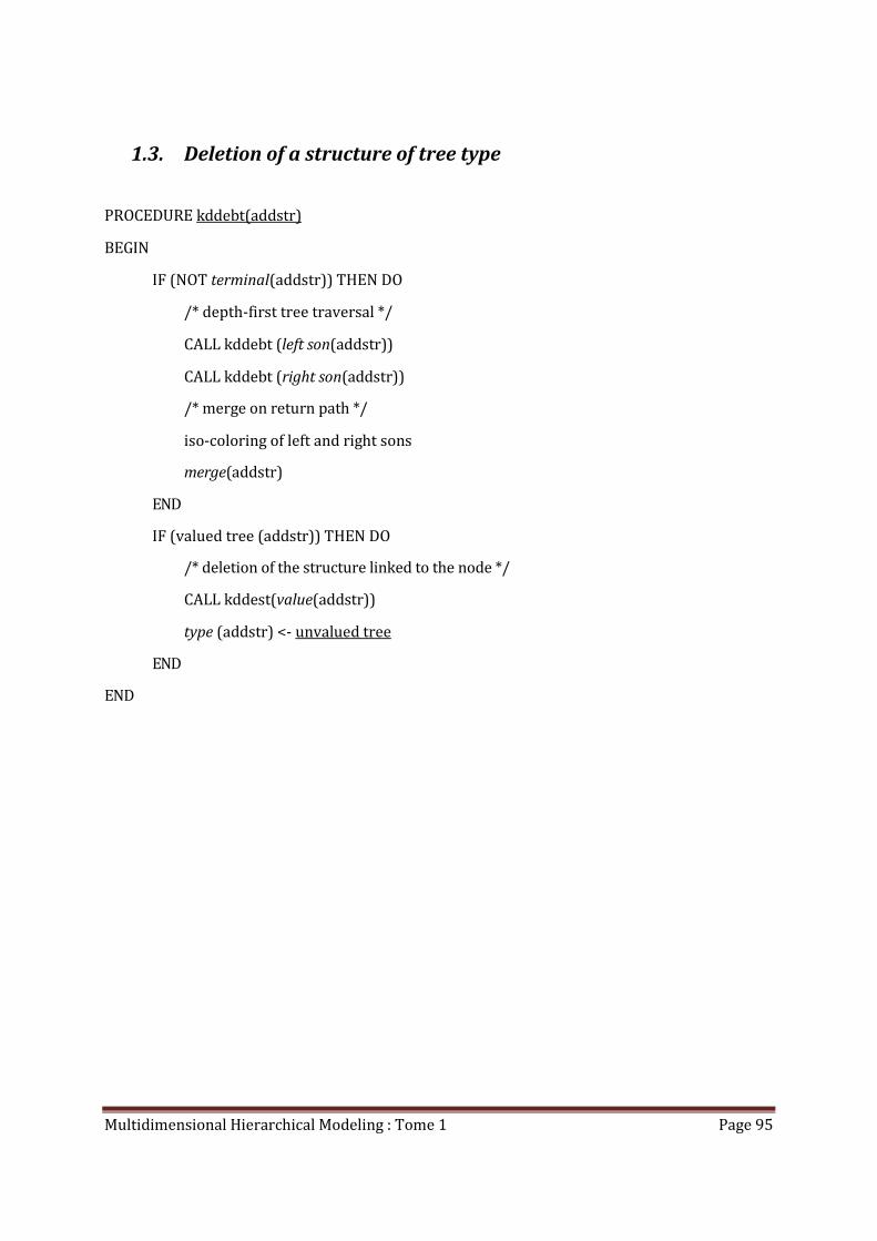
Multidimensional Hierarchical Modeling : Tome 1 Page 95
1.3. Deletion of a structure of tree type
PROCEDURE kddebt(addstr)
BEGIN
IF (NOT terminal(addstr)) THEN DO
/* depth-first tree traversal */
CALL kddebt (left son(addstr))
CALL kddebt (right son(addstr))
/* merge on return path */
iso-coloring of left and right sons
merge(addstr)
END
IF (valued tree (addstr)) THEN DO
/* deletion of the structure linked to the node */
CALL kddest(value(addstr))
type (addstr) <- unvalued tree
END
END
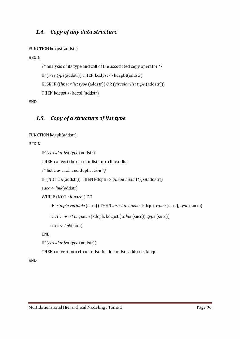
Multidimensional Hierarchical Modeling : Tome 1 Page 96
1.4. Copy of any data structure
FUNCTION kdcpst(addstr)
BEGIN
/* analysis of its type and call of the associated copy operator */
IF (tree type(addstr)) THEN kddpst <- kdcpbt(addstr)
ELSE IF ((linear list type (addstr)) OR (circular list type (addstr)))
THEN kdcpst <- kdcpli(addstr)
END
1.5. Copy of a structure of list type
FUNCTION kdcpli(addstr)
BEGIN
IF (circular list type (addstr))
THEN convert the circular list into a linear list
/* list traversal and duplication */
IF (NOT nil(addstr)) THEN kdcpli <- queue head (type(addstr))
succ <- link(addstr)
WHILE (NOT nil(succ)) DO
IF (simple variable (succ)) THEN insert in queue (kdcpli, value (succ), type (succ))
ELSE insert in queue (kdcpli, kdcpst (value (succ)), type (succ))
succ <- link(succ)
END
IF (circular list type (addstr))
THEN convert into circular list the linear lists addstr et kdcpli
END
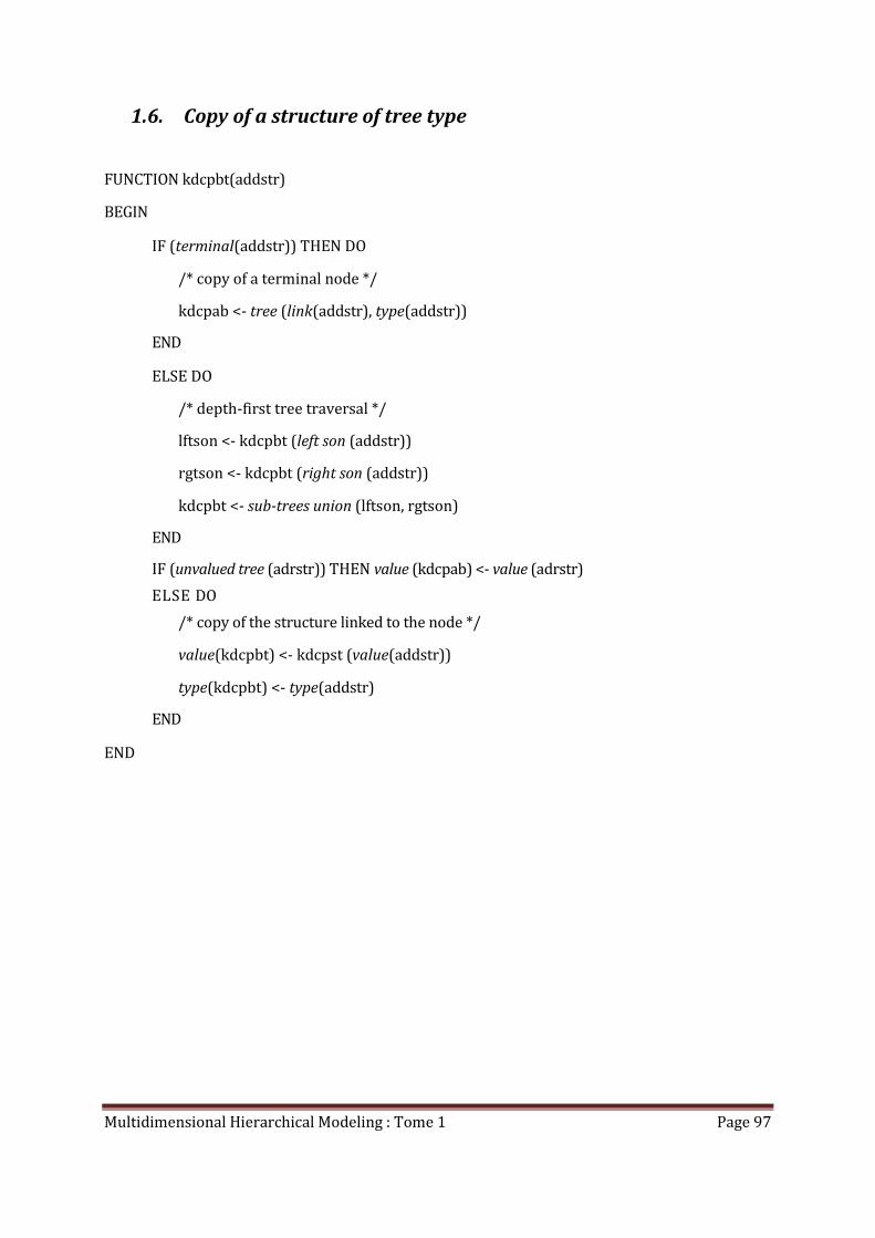
Multidimensional Hierarchical Modeling : Tome 1 Page 97
1.6. Copy of a structure of tree type
FUNCTION kdcpbt(addstr)
BEGIN
IF (terminal(addstr)) THEN DO
/* copy of a terminal node */
kdcpab <- tree (link(addstr), type(addstr))
END
ELSE DO
/* depth-first tree traversal */
lftson <- kdcpbt (left son (addstr))
rgtson <- kdcpbt (right son (addstr))
kdcpbt <- sub-trees union (lftson, rgtson)
END
IF (unvalued tree (adrstr)) THEN value (kdcpab) <- value (adrstr)
ELSE DO
/* copy of the structure linked to the node */
value(kdcpbt) <- kdcpst (value(addstr))
type(kdcpbt) <- type(addstr)
END
END
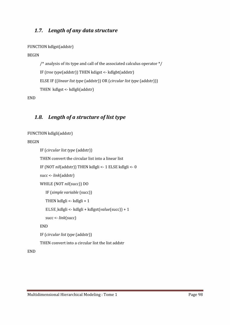
Multidimensional Hierarchical Modeling : Tome 1 Page 98
1.7. Length of any data structure
FUNCTION kdlgst(addstr)
BEGIN
/* analysis of its type and call of the associated calculus operator */
IF (tree type(addstr)) THEN kdigst <- kdlgbt(addstr)
ELSE IF ((linear list type (addstr)) OR (circular list type (addstr)))
THEN kdlgst <- kdlgli(addstr)
END
1.8. Length of a structure of list type
FUNCTION kdlgli(addstr)
BEGIN
IF (circular list type (addstr))
THEN convert the circular list into a linear list
IF (NOT nil(addstr)) THEN kdlgli <- 1 ELSE kdlgli <- 0
succ <- link(addstr)
WHILE (NOT nil(succ)) DO
IF (simple variable (succ))
THEN kdlgli <- kdlgli + 1
ELSE kdlgli <- kdlgli + kdlgst(value(succ)) + 1
succ <- link(succ)
END
IF (circular list type (addstr))
THEN convert into a circular list the list addstr
END

Multidimensional Hierarchical Modeling : Tome 1 Page 99
1.9. Length of a structure of tree type
FUNCTION kdlgbt(addstr)
BEGIN
IF (terrninal (addstr)) THEN kdlgbt <- 1
ELSE DO
/* depth-first tree traversal */
lftlgt <- kdlgbt (left son (addstr))
rgtlgt <- kdlgbt (right son (addstr))
kdlgbt <- lftlgt + rgtlgt +1
END
IF (valued tree (addstr)) THEN DO
/* length calculus of the structure linked to the node */
kdlgbt <- kdlgbt + kdlgst(value(addstr))
END
END

Multidimensional Hierarchical Modeling : Tome 1 Page 100

Multidimensional Hierarchical Modeling : Tome 1 Page 101
2. Tree generation by vector addition
root : root of the tree to be enriched
vecthd : head of the integer vector to be added
vector: head of the real vector to be added
dimens : dimension of the modeling space
precis : computation precision
depth : computation depth
level : level reached in the tree
side: descent side in the tree
minroo : minimum coordinates list of the root
maxroo : maximum coordinates list of the root
xmin : minimum coordinate of the root
xmax : maximum coordinate of the root
xvec : vector coordinate to be added
xctr : center coordinate of the root

Multidimensional Hierarchical Modeling : Tome 1 Page 102
2.1. Addition of an integer vector to a tree
PROCEDURE kdaivt(root ,vecthd, dimens, precis)
BEGIN
/* initialization of computing parameters */
depth <- dimens * precis, level <- 0
/* recursive computing unit */
PROCEDURE kdaivt (root, vecthd , level)
BEGIN
IF (level=depth) THEN blacken (root)
ELSE DO
/* tree descent driven by the vector coordinates */
side <- extraction of most significant bit of current coordinate,
right binary shift of this one,
and coordinate circular shift of vector(vecthd)
IF (terminal(root)) THEN fission(root)
CALL kdaivt(son(root, side), vecthd, level + 1)
merge (root)
END
EN D
EN D
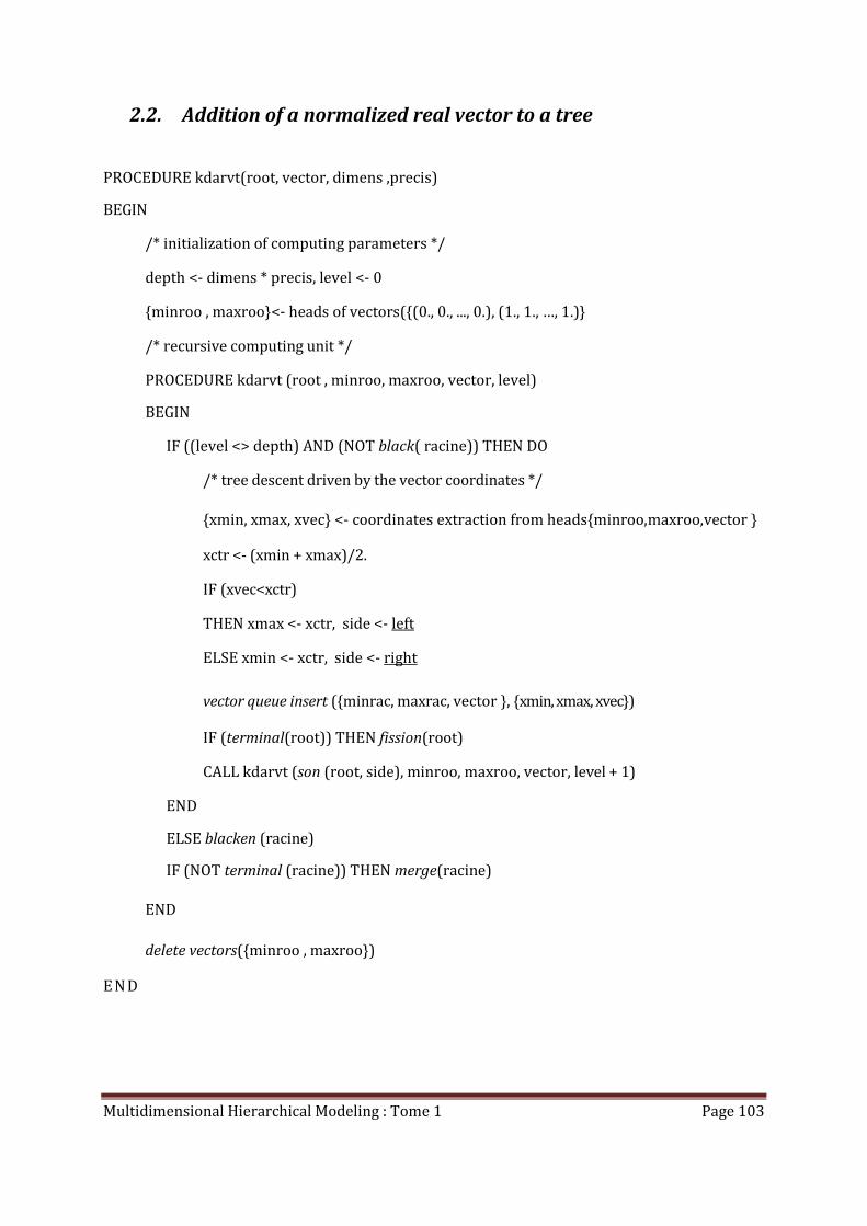
Multidimensional Hierarchical Modeling : Tome 1 Page 103
2.2. Addition of a normalized real vector to a tree
PROCEDURE kdarvt(root, vector, dimens ,precis)
BEGIN
/* initialization of computing parameters */
depth <- dimens * precis, level <- 0
{minroo , maxroo}<- heads of vectors({(0., 0., ..., 0.), (1., 1., …, 1.)}
/* recursive computing unit */
PROCEDURE kdarvt (root , minroo, maxroo, vector, level)
BEGIN
IF ((level <> depth) AND (NOT black( racine)) THEN DO
/* tree descent driven by the vector coordinates */
{xmin, xmax, xvec} <- coordinates extraction from heads{minroo,maxroo,vector }
xctr <- (xmin + xmax)/2.
IF (xvec<xctr)
THEN xmax <- xctr, side <- left
ELSE xmin <- xctr, side <- right
vector queue insert ({minrac, maxrac, vector }, {xmin, xmax, xvec})
IF (terminal(root)) THEN fission(root)
CALL kdarvt (son (root, side), minroo, maxroo, vector, level + 1)
END
ELSE blacken (racine)
IF (NOT terminal (racine)) THEN merge(racine)
END
delete vectors({minroo , maxroo})
E N D

Multidimensional Hierarchical Modeling : Tome 1 Page 104
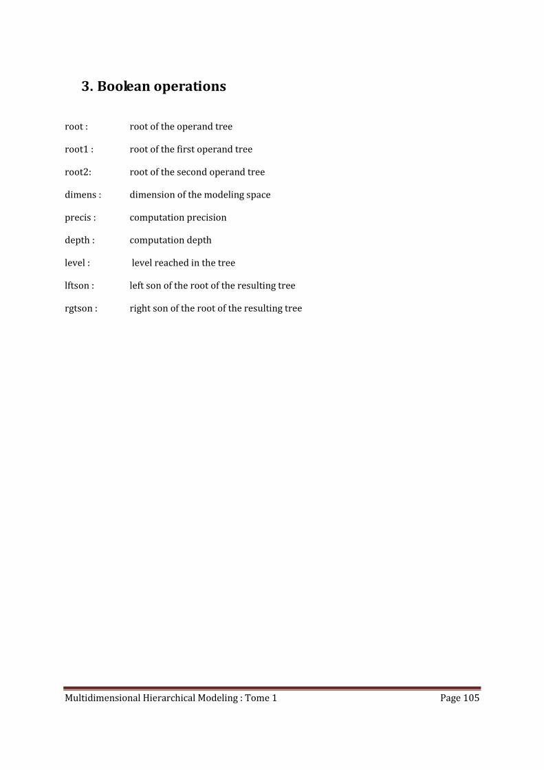
Multidimensional Hierarchical Modeling : Tome 1 Page 105
3. Boolean operations
root : root of the operand tree
root1 : root of the first operand tree
root2: root of the second operand tree
dimens : dimension of the modeling space
precis : computation precision
depth : computation depth
level : level reached in the tree
lftson : left son of the root of the resulting tree
rgtson : right son of the root of the resulting tree

Multidimensional Hierarchical Modeling : Tome 1 Page 106
3.1. Assertion of a binary tree
FUNCTION kdass(racine, dimens, precis)
BEGIN
/* initialization of computing parameters */
depth <- dimens * precis, level <- 0
/* recursive computing unit */
FUNCTION kdass(root, level)
BEGIN
IF ((NOT terminal (root)) AND (level <> depth)) THEN DO
/* depth-first tree traversal */
lftson <- kdass(left son(root), level + 1)
rgtson <- kdass(right son(root), level + 1)
kdass <- sub-trees union(lftson, rgtson)
END
ELSE DO
/* assertion of the node reached in the tree */
IF (white (root))
THEN kdass <- tree (white)
ELSE kdass <- tree (black)
END
/* merge of sons’ nodes on return path */
IF (NOT terminal (kdass)) THEN merge (kdass)
END
EN D
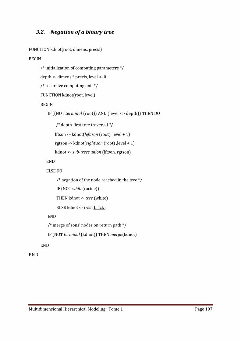
Multidimensional Hierarchical Modeling : Tome 1 Page 107
3.2. Negation of a binary tree
FUNCTION kdnot(root, dimens, precis)
BEGIN
/* initialization of computing parameters */
depth <- dimens * precis, level <- 0
/* recursive computing unit */
FUNCTION kdnot(root, level)
BEGIN
IF ((NOT terminal (root)) AND (level <> depth)) THEN DO
/* depth-first tree traversal */
lftson <- kdnot(left son (root), level + 1)
rgtson <- kdnot(right son (root) ,level + 1)
kdnot <- sub-trees union (lftson, rgtson)
END
ELSE DO
/* negation of the node reached in the tree */
IF (NOT white(racine))
THEN kdnot <- tree (white)
ELSE kdnot <- tree (black)
END
/* merge of sons’ nodes on return path */
IF (NOT terminal (kdnot)) THEN merge(kdnot)
END
EN D
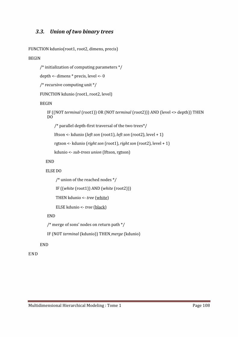
Multidimensional Hierarchical Modeling : Tome 1 Page 108
3.3. Union of two binary trees
FUNCTION kdunio(root1, root2, dimens, precis)
BEGIN
/* initialization of computing parameters */
depth <- dimens * precis, level <- 0
/* recursive computing unit */
FUNCTION kdunio (root1, root2, level)
BEGIN
IF ((NOT terminal (root1)) OR (NOT terminal (root2))) AND (level <> depth)) THEN DO
/* parallel depth-first traversal of the two trees*/
lftson <- kdunio (left son (root1), left son (root2), level + 1)
rgtson <- kdunio (right son (root1), right son (root2), level + 1)
kdunio <- sub-trees union (lftson, rgtson)
END
ELSE DO
/* union of the reached nodes */
IF ((white (root1)) AND (white (root2)))
THEN kdunio <- tree (white)
ELSE kdunio <- tree (black)
END
/* merge of sons’ nodes on return path */
IF (NOT terminal (kdunio)) THEN merge (kdunio)
END
EN D
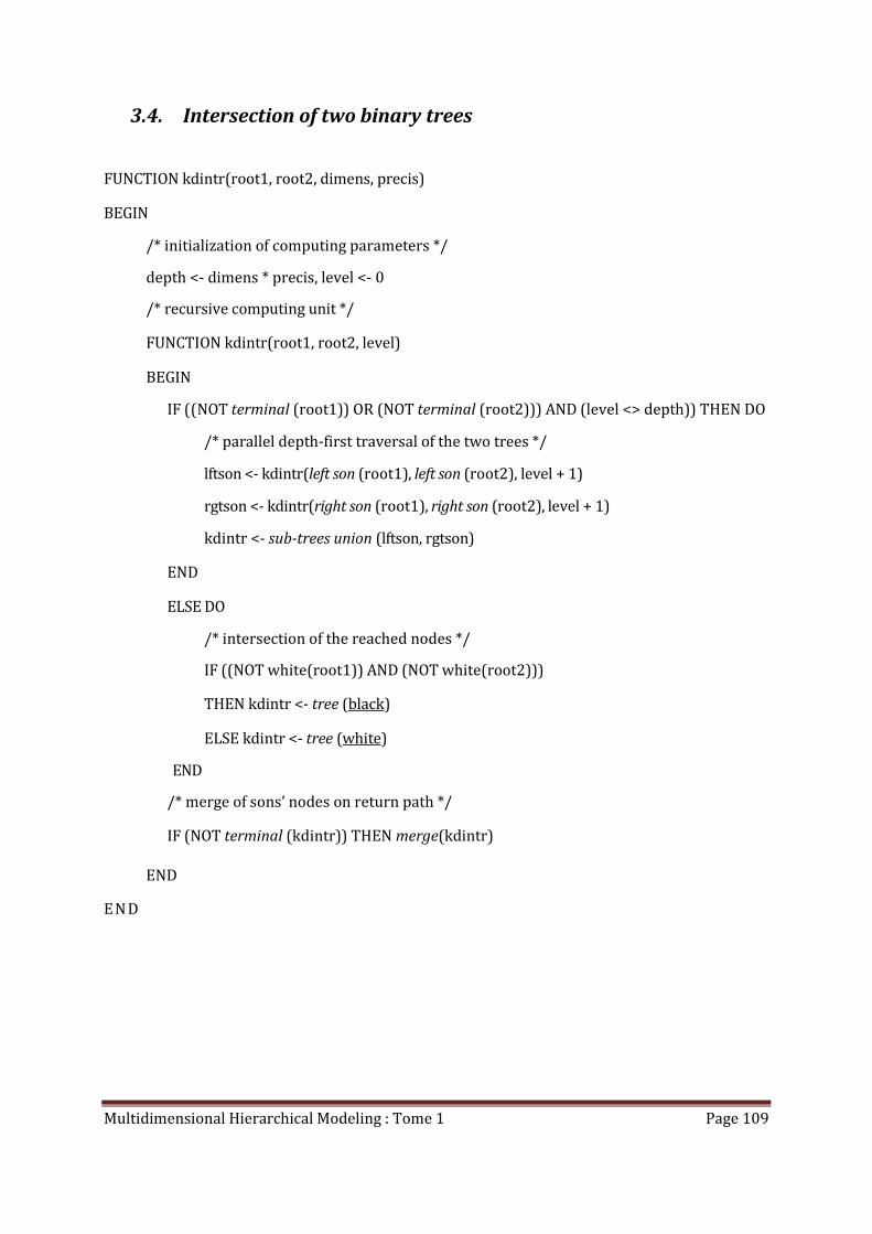
Multidimensional Hierarchical Modeling : Tome 1 Page 109
3.4. Intersection of two binary trees
FUNCTION kdintr(root1, root2, dimens, precis)
BEGIN
/* initialization of computing parameters */
depth <- dimens * precis, level <- 0
/* recursive computing unit */
FUNCTION kdintr(root1, root2, level)
BEGIN
IF ((NOT terminal (root1)) OR (NOT terminal (root2))) AND (level <> depth)) THEN DO
/* parallel depth-first traversal of the two trees */
lftson <- kdintr(left son (root1), left son (root2), level + 1)
rgtson <- kdintr(right son (root1), right son (root2), level + 1)
kdintr <- sub-trees union (lftson, rgtson)
END
ELSE DO
/* intersection of the reached nodes */
IF ((NOT white(root1)) AND (NOT white(root2)))
THEN kdintr <- tree (black)
ELSE kdintr <- tree (white)
END
/* merge of sons’ nodes on return path */
IF (NOT terminal (kdintr)) THEN merge(kdintr)
END
EN D
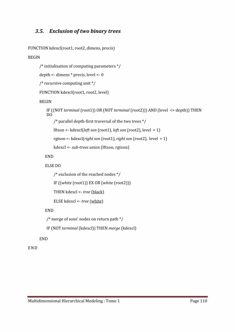
Multidimensional Hierarchical Modeling : Tome 1 Page 110
3.5. Exclusion of two binary trees
FUNCTION kdexcl(root1, root2, dimens, precis)
BEGIN
/* initialization of computing parameters */
depth <- dimens * precis, level <- 0
/* recursive computing unit */
FUNCTION kdexcl(root1, root2, level)
BEGIN
IF ((NOT terminal (root1)) OR (NOT terminal (root2))) AND (level <> depth)) THEN DO
/* parallel depth-first traversal of the two trees */
lftson <- kdexcl(left son (root1), left son (root2), level + 1)
rgtson <- kdexcl(right son (root1), right son (root2), level + 1)
kdexcl <- sub-trees union (lftson, rgtson)
END
ELSE DO
/* exclusion of the reached nodes */
IF ((white (root1)) EX OR (white (root2)))
THEN kdexcl <- tree (black)
ELSE kdexcl <- tree (white)
END
/* merge of sons’ nodes on return path */
IF (NOT terminal (kdexcl)) THEN merge (kdexcl)
END
EN D
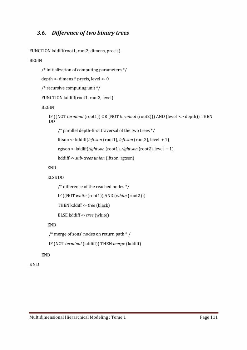
Multidimensional Hierarchical Modeling : Tome 1 Page 111
3.6. Difference of two binary trees
FUNCTION kddiff(root1, root2, dimens, precis)
BEGIN
/* initialization of computing parameters */
depth <- dimens * precis, level <- 0
/* recursive computing unit */
FUNCTION kddiff(root1, root2, level)
BEGIN
IF ((NOT terminal (root1)) OR (NOT terminal (root2))) AND (level <> depth)) THEN DO
/* parallel depth-first traversal of the two trees */
lftson <- kddiff(left son (root1), left son (root2), level + 1)
rgtson <- kddiff(right son (root1), right son (root2), level + 1)
kddiff <- sub-trees union (lftson, rgtson)
END
ELSE DO
/* difference of the reached nodes */
IF ((NOT white (root1)) AND (white (root2)))
THEN kddiff <- tree (black)
ELSE kddiff <- tree (white)
END
/* merge of sons’ nodes on return path * /
IF (NOT terminal (kddiff)) THEN merge (kddiff)
END
EN D

Multidimensional Hierarchical Modeling : Tome 1 Page 112

Multidimensional Hierarchical Modeling : Tome 1 Page 113
4. Handling of slices parallel to the axes
spacro : root of the space to be processed
dimesp : dimension of the modeled space
slicro : root of the slice to be inserted
dimslc : dimension of the slice space
slvcro : tree root of the slice coordinates vector
codslc : dimension of the tree of the slice coordinates (codimension of the slice in the space to be processed)
slcvec : vector head of the slice axes (for each coordinate of the space to be processed, it indicates if the axis is a slice axis or not)
precis : computation precision
slaxis : axis in the process of analysis belonging to the slice axes vector
depth : computation depth
level : level reached in the tree
lftson : left son in the slice
rgtson : right son in the slice
intrsc : intersection of the slice with the slice coordinates
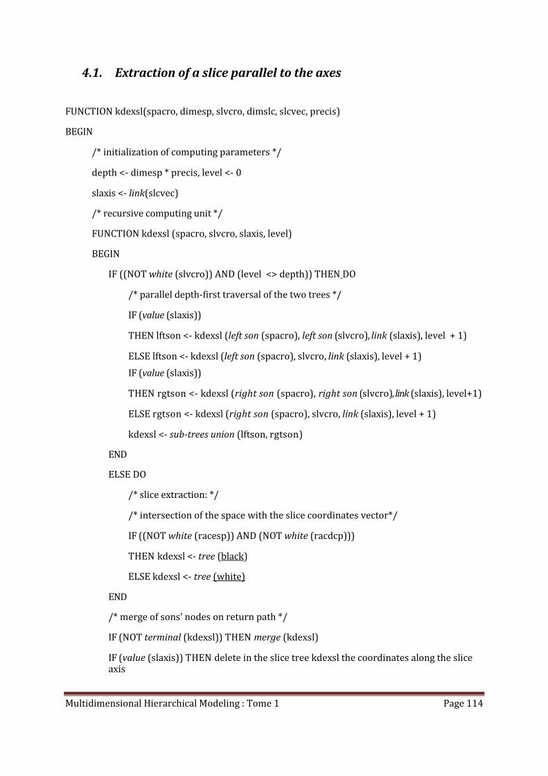
Multidimensional Hierarchical Modeling : Tome 1 Page 114
4.1. Extraction of a slice parallel to the axes
FUNCTION kdexsl(spacro, dimesp, slvcro, dimslc, slcvec, precis)
BEGIN
/* initialization of computing parameters */
depth <- dimesp * precis, level <- 0
slaxis <- link(slcvec)
/* recursive computing unit */
FUNCTION kdexsl (spacro, slvcro, slaxis, level)
BEGIN
IF ((NOT white (slvcro)) AND (level <> depth)) THEN DO
/* parallel depth-first traversal of the two trees */
IF (value (slaxis))
THEN lftson <- kdexsl (left son (spacro), left son (slvcro), link (slaxis), level + 1)
ELSE lftson <- kdexsl (left son (spacro), slvcro, link (slaxis), level + 1)
IF (value (slaxis))
THEN rgtson <- kdexsl (right son (spacro), right son (slvcro), link (slaxis), level+1)
ELSE rgtson <- kdexsl (right son (spacro), slvcro, link (slaxis), level + 1)
kdexsl <- sub-trees union (lftson, rgtson)
END
ELSE DO
/* slice extraction: */
/* intersection of the space with the slice coordinates vector*/
IF ((NOT white (racesp)) AND (NOT white (racdcp)))
THEN kdexsl <- tree (black)
ELSE kdexsl <- tree (white)
END
/* merge of sons’ nodes on return path */
IF (NOT terminal (kdexsl)) THEN merge (kdexsl)
IF (value (slaxis)) THEN delete in the slice tree kdexsl the coordinates along the slice axis
Multidimensional Hierarchical Modeling : Tome 1 Page 115
EN D
E N D
4.2. Insertion of a slice parallel to the axes
PROCEDURE kdinsl(spacro, slicro, dimslc, slvcro, codslc, slcvec, precis)
BEGIN
/* initialization of computing parameters */
depth <- (dimslc + codslc) * precis, level <- 0
slaxis <- link (slcvec)
/* recursive computing unit */
PROCEDURE kdinsl (spacro, slicro, slvcro, slaxis, level)
BEGIN
IF ((NOT white( slicro)) AND (level <> depth)) THEN DO
/* parallel depth-first traversal of the three trees */
IF (value (slaxis))
THEN CALL kdinsl (left son ((spacro), slicro, left son (slvcro), link (slcvec), level + 1)
ELSE CALL kdinsl (left son (spacro), left son (slicro), slvcro, link (slcvec), level + 1)
IF (value (slaxis))
THEN CALL kdinsl (right son (spacro), slicro, right son (slvcro), link (slcvec), level + 1)
ELSE CALL kdinsl (right son (spacro), right son (slicro), slvcro, link (slcvec), level + 1)
E N D

Multidimensional Hierarchical Modeling : Tome 1 Page 116
ELSE DO
IF (level=depth) THEN DO
IF (NOT terminal (spacro)) THEN put at terminal state the sub-tree spacro
/* slice insertion: */
/* computation of the intersection of the slice with the slice coordinates vector */
IF ((NOT white (slicro)) AND (NOT white (slvcro)))
THEN intrsc <- black
ELSE intrsc <- white
/* union of the space with the result of the intersection */
IF ((white (spacro)) AND (white (intrsc)))
THEN whiten (spacro)
ELSE blacken (spacro)
E N D
END
/* merge of sons’ nodes on return path */
IF (NOT terminal (spacro)) THEN merge (spacro)
END
E N D
Multidimensional Hierarchical Modeling : Tome 1 Page 117
5. Building of the tree of a polyhedron
polyed : list of the polyhedron vertices
minhyp : list of the polyhedron lower faces
maxhyp : list of the polyhedron higher faces
dimens : dimension of the modeled space
precis : computation precision
depth : computation depth
level : level reached in the tree
{polspc, minspc, maxspc} : vertices and faces of a block coming from the regular dividing de
of the modeled space
inters : intersection indicator of two polyhedrons
incp12 : inclusion of the first polyhedron into the second one
incp21 : inclusion of the second polyhedron into the first one
{polye1, minhp1, maxhp1} : vertices and faces of the first polyhedron
{polye2, minhp2, maxhp2} : vertices and faces of the second polyhedron
nudim : number of the processed dimension
nulspc : inclusion indicator of a polyhedron into a hyper-plane
negspc : inclusion indicator of a polyhedron into a negative half-space
posspc : inclusion indicator of a polyhedron into a positive half-space
hyplan : hyper-plane partitioning the spce onto two half-spaces
nuvert : vertex number
order : butterfly size
nubut : bufferfly number
dimhom : dimension of the space in homogenous coordinates
nuplan : plane number in the faces list
Multidimensional Hierarchical Modeling : Tome 1 Page 118
{pollft, minlft, maxlft} : vertices and faces of the left half-polyhedron
{polrgt, minrgt, maxrgt} : vertices and faces of the right half-polyhedron
5.1. Building of the tree of a polyhedron defined by its vertices and
its faces
FUNCTION kdpolt(polyed, minhyp, maxhyp, dimens, precis)
BEGIN
/* building initialization */
/* computation of the vertices and the faces of the block linked to the root */
polspc <- unitary space vertices (dimens)
minspc <- unitary space lower hyperplanes (dimens)
maxspc <- unitary space higher hyperplanes (dimens)
depth <- dimens * precis, level <- 0
/* recursive computing unit */
FUNCTION kdpolt ([polyed, minhyp, maxhyp,] polspc, minspc, maxspc, level)
BEGIN
/* hierarchical traversal of the inside and the boundary of the polyhedron */
intersection evaluation of the block linked to the node and of the polyhedron (polspc, minspc, maxspc, polyed, minhyp, maxhyp)
IF ((level <> depth) AND ((intersection) AND (block ⊄ polyhedron))) THEN DO
/* the block linked to the node is on the boundary of the polyhedron */
{pollft, polrgt} <- vertex-based polyhedron division (polspc)
{minlft , maxlft, minrgt, maxrgt}<- face-based polyhedron division (minspc, maxspc)
lftson<- kdpolt (pollft, minlft, maxlft , level + 1)
rgtson <- kdpolt (polrgt, minrgt, maxrgt, level + 1)
kdpolt <- sub-trees union (lftson, rgtson)
merge (kdcvap)
END
Multidimensional Hierarchical Modeling : Tome 1 Page 119
ELSE DO
/*covering at the required precision or inclusion of the block linked to the node into the polyhedron*/
IF (((level = depth) AND (intersection)) OR (block ⊂ polyhedron))
THEN kdpolt <- tree (black).
ELSE kdpolt <- tree (white)
END
delete block {polspc, minspc, maxspc}
END
END
5.2. Intersection evaluation of two convex polyhedrons
PROCEDURE kdiecp(inters, incp12, incp21, polye1, minhp1, maxhp1, polye2, minhp2,
maxhp2, dimens)
BEGIN
/* the intersection is not validated when all the vertices of a polyhedron belong to the half-space related to one of the hyperplanes belonging to the other polyhedron */
/* a polyhedron is included into the other polyhedron, when all its vertices belong to the internal half-spaces defined by the hyperplanes of the other polyhedron */
inters <- true
/* examination of the faces of the first polyhedron */
Incp12 <- true
/* examination of the lower hyperplanes of the first polyhedron */
FOR nudim = 1 TO dimens DO
position evaluation of a polyhedron compared to a hyperplane (polye2, minhp1(nudim), inside hyperplane, left space, right space)
/* the left space is outside the poylhedron, the right space is inside*/
IF (NOT inside hyperplane) THEN DO
IF (NOT right space) THEN incp12 <- false
IF (left space) THEN inters <- false
END
Multidimensional Hierarchical Modeling : Tome 1 Page 120
END
/* examination of the higher hyperplanes of the first polyhedron */
FOR nudim = 1 TO dimens DO
position evaluation of a polyhedron compared to a hyperplane (polye2, maxhp1(nudim), inside hyperplane, left space, right space)
/* the left space is inside the polyhedron, the right space is outside */
IF (NOT inside hyperplane) THEN DO
IF (NOT left space) THEN incp12 <- false
IF (right space) THEN inters <- false
END
END
/* examination of the faces of the second polyhedron */
incp21 <- true
/* examination of the lower hyperplanes of the second polyhedron */
FOR nudim = 1 TO dimens DO
position evaluation of a polyhedron compared to a hyperplane (polye1, minhp2(nudim), inside hyperplane, left space, right space)
IF (NOT inside hyperplane) THEN DO
IF (NOT right space) THEN incp21 <- false
IF (left space) THEN inters <- false
END
END
/* examination of the higher hyperplanes of the second polyhedron */
FOR nudim = 1 TO dimens DO
position evaluation of a polyhedron compared to a hyperplane (polye1, maxhp2(nudim), inside hyperplane, left space, right space)
IF (NOT inside hyperplane) THEN DO
IF (NOT left space) THEN alors incp21 <- false
IF (right space) THEN alors inters <- false
END
END
overriding of inclusion indicators when not any intersection
Multidimensional Hierarchical Modeling : Tome 1 Page 121
END
5.3. Position evaluation of a polyhedron compared to a hyperplane
PROCEDURE kdpohp(nulspc, negspc, posspc, polyed, hyplan, dimens)
BEGIN
/*test initialization */
nulspc, negspc, posspc <- true
/* examination of polyhedron vertices */
FOR nuvert = 1 TO 2**dimens DO
posit <- 0.
/* examination of vertex coordinates */
FOR nudim = 1 TO dimens DO
posit <- posit + (polyed(nuvert, nudim) * hyplan(nudim))
END
posit <- posit + hyplan(nudim + 1)
IF (posit=0.) THEN nulspc <- false
IF (posit>0.) THEN negspc <- false
IF (posit<0.) THEN posspc <- false
E N D
END
Multidimensional Hierarchical Modeling : Tome 1 Page 122
5.4. Vertex-based polyhedron division into two half-polyhedrons
PROCEDURE kddivp(polyed, pollft, poldrt, order, dimens)
BEGIN
/* update of the size of decomposition butterfly lattices */
nudim <- dimens – LOG2(order)
nudim <- MOD(nudim + 1, dimens) + 1
order <- 2**(dimens - nudim)
/* polyhedron analysis according butterflies of order vertices */
FOR nubut = 1 TO MOD(2**dimens, order) DO
/* division of the butterfly vertices */
FOR nuvert = ((nubut - 1) * order) TO (nubut * order) DO
nuver1 <- nuvert
nuver2 <- nuvert + order
/* coordinates division */
FOR nudim = 1 TO dimens DO
pollft(nuver1, nudim) <- polyed (nuver1, nudim)
polrgt(nuver2, nudim)
<- (polyed (nuver1, nudim) + polyed (nuver2, nudim))/2.
polrgt (nusom1, nudim) <- pollft (nuver2, nudim)
polrgt (nusom1, nudim) <- polyed (nuver2, nudim)
E N D
EN D
EN D
EN D
Multidimensional Hierarchical Modeling : Tome 1 Page 123
5.5. Face-based polyhedron division into two half-polyhedrons
PROCEDURE kddivh(minhyp, maxhyp, minlft, maxlft, minrgt, maxrgt, npldiv, dimens)
BEGIN
/*space dimension in homogenous coordinates*/
dimhom <- dimens + 1
/* polyhedron division in two halves separated by the median hyperplane of the npldiv-th lower and higher faces */
FOR nuplan = 1 TO dimhom DO
/* division of polyhedron faces */
FOR nudim = 1 TO dimhom DO
/* division of faces into homogenous coordinates */
minlft(nuplan, nudim) <- minhyp(nuplan, nudim)
IF (nuplan=npldiv) THEN DO
maxlft(nuplan, nudim) <- (minhyp(nuplan,
nudim)+maxhyp(nuplan, nudim))/2.
minrgt(nuplan, nudim) <- maxlft(nuplan, nudim)
END
ELSE DO
maxlft(nuplan, nudim) <- maxhyp(nuplan ,nudim)
minrgt(nuplan, nudim) <- minhyp(nuplan, nudim)
END
maxrgt(nuplan, nudim) <- maxhyp(nuplan, nudim)
END
END
END

Multidimensional Hierarchical Modeling : Tome 1 Page 124

Multidimensional Hierarchical Modeling : Tome 1 Page 125
6. Tree homogenous transformation
root : root of the tree to be transformed
polyed : list of the polyhedron vertices
minhyp : list of the polyhedron lower faces
maxhyp : list of the polyhedron higher faces
dimens : space dimension
prec1 : analysis precision
prec2 : building precision
polybt : tree of the transformation polyhedron
trfroo : root of the transformed tree
depth : computation depth
level : level reached in the tree
{polroo, minroo, maxroo} : vertices and faces of the block linked to a node
{pollft, minlft, maxlft} : left half-polyhedron
{polrgt, minrgt, maxrgt} : right half-polyhedron
{polblo, minblo, maxblo} : vertices and faces coming from a terminal node
Multidimensional Hierarchical Modeling : Tome 1 Page 126
6.1. Computation of the transformed image of a tree according to a
homogenous transformation
FUNCTION kdthom(root, polyed, minhyp, maxhyp, dimens ,prec1, prec2)
BEGIN
kdthom <- tree (white)
polybt <- tree of the polyhedron (polyed, minhyp, maxhyp)
analysis and non linear transform of the tree (root, kdthom, polybt, polyed, minhyp, maxhyp, dimens, prec1, prec2)
delete tree (polybt)
EN D
/* Analysis of a tree in order to further compute its transformed release by a non linear transformation*/
PROCEDURE kdanlt(root, trfroo, polybt, polyed, minhyp, maxhyp, dimens, prec1, prec2)
BEGIN
/* analysis initialization */
depth <- dimens * prec1, level <- 0
polroo <- unitary space vertices (dimens)
minroo <- unitary space lower hyperplanes (dimens)
maxroo <- unitary space higher hyperplanes (dimens)
/* recursive computing unit */
PROCEDURE kdanlt (root, polybt, polroo, minroo, maxroo,[ trfroo, polyed, minhyp, maxhyp,] level)
BEGIN
/*search of black terminal nodes included in the polyhedron/*
IF ((level <> depth) AND (NOT white (polybt)) AND (NOT white (root)))
THEN DO

Multidimensional Hierarchical Modeling : Tome 1 Page 127
IF ((NOT terminal (polybt)) OR (NOT terminal (root)))
THEN DO
/*parallel depth-first traversal of the tree to be transformed and the tree of the polyhedron*/
{pollft, polrgt} <- vertex-based polyhedron division (polroo)
{minlft, maxlft, minrgt, maxrgt} <- face-based polyhedron division (minroo,
maxroo)
appel kdanlt (left son (root), left son (polybt), pollft, minlft, maxlft, level + 1)
appel kdanlt (right son (root), right son (polybt), poldrt, minrgt, maxrgt, level + 1)
END
ELSE DO
/* black block included in the polyhedron */
decomposition of the block in the resulting space(trfroo, polyed, minhyp, maxhyp, polroo, minroo, maxroo, dimens, prec2)
END
END
ELSE DO
/* analysis resolution reached */
IF ((NOT white (polybt)) AND (NOT white (root)))
THEN decomposition of the block in the resulting space (trfroo, polyed, minhyp, maxhyp, polroo, minroo, maxroo, dimens, prec2)
END
/* tree traversal return path */
delete polyhedron {polroo, minroo, maxroo}
END
END
Multidimensional Hierarchical Modeling : Tome 1 Page 128
/* Decomposition of a terminal block in the image space of a geometric transformation */
PROCEDURE kdgtbl(root, polyed, minhyp, maxhyp, polblo, minblo, maxblo, dimens, precis)
BEGIN
/* decomposition initialization */
depth <- dimens * precis, level <-0
/* recursive computing unit */
PROCEDURE kdtgbl(root, polyed, minhyp, maxhyp,[polblo, minblo, maxblo,] level)
BEGIN
intersection evaluation of the terminal block with the transform polyhedron (polblo, minblo, maxblo, polyed, minhyp, maxhyp)
IF ((level <> depth) AND (NOT black (root))AND ((intersection) AND (polyhedron ⊄ block))) THEN DO
/* the transform polyhedron is not included in the terminal block, it will then divided into two halves */
{pollft, polrgt} <- vertex-based polyhedron division (polyed)
{minlft, maxlft, minrgt, maxrgt} <- face-based polyhedron division (minhyp, maxhyp)
IF (terminal(root)) THEN fission (root)
CALL kdgtbl (left son (root), pollft, minlft, maxlft, level + 1)
CALL kdgtbl (right son (root), polrgt, minrgt, maxrgt, level + 1)
END
ELSE DO
/* the polyhedron included in the block is a black node of the transformed tree */
IF ((NOT black (root))AND (intersection)) THEN blacken (root)
END
/* tree traversal return path */
IF (NOT terminal (root)) THEN merge (root)
IF (level<>0) THEN delete polyhedron(polyed,minhyp, maxhyp)
END
END
Multidimensional Hierarchical Modeling : Tome 1 Page 129
6.2. Computation of the transformed image of a tree according to a
homogenous transformation (fast transform)
FUNCTION kdfthm(root, polyed, minhyp, maxhyp, dimens, prec1, prec2)
BEGIN
polybt <- tree of the polyhedron (polyed, minhyp, maxhyp)
kdfthm <- tree (white)
value(kdfthm) <- {polyed, minhyp, maxhyp}
analysis and non linear transform of the tree, fast transform (racine, kdfthm, polybt, dimens, prec1, prec2)
devaluate tree (kdfthm)
delete tree (polybt)
f in
/* Analysis of a tree in order to further compute its transformed release by a non linear
transformation (fast transform)*/
PROCEDURE kdfanl(root, trfroo, polybt, dimens, prec1, prec2)
This procedure is identical to kdanlt, apart that:
− the transformation polyhedron {polyed ,minhyp, maxhyp} do not more appear
explicitly among the call parameters, because it is stored in the root of the
transformed tree;
− the block decomposition in the image space is replaced by its fast version.
Multidimensional Hierarchical Modeling : Tome 1 Page 130
/* Decomposition of a terminal block in the image space of a geometric transformation (fast
version)*/
PROCEDURE kdfgtb(root, polblo, minblo, maxblo, dimens, precis)
BEGIN
/* decomposition initialization */
depth <- dimens * precis, level <-0
/* recursive computing unit */
PROCEDURE kdtgbr( racine ,[polblo , minblo , maxblo] level)
BEGIN
{polyed, minhyp, maxhyp} <- value(racine)
intersection evaluation of the terminal block with the transform polyhedron (polblo, minblo, maxblo, polyed, minhyp, maxhyp)
IF ((level <> depth) AND (NOT black (root)) AND ((intersection) AND (pyhedron ⊄ block))) THEN DO
/* the transform polyhedron is not included in the terminal block */
IF (terminal (root)) THEN DO
merge (root)
/*division of the transform polyhedron into two halves, and store them into the root children*/
{pollft, polrgt} <- vertex-based polyhedron division (polyed)
{minlft, maxlft, minrgt, maxrgt} <- face-based polyhedron division (minhyp, maxhyp)
value(left son(root)) <- { pollft, minlft, maxlft}
value(right son(root)) <- { polrgt, minrgt, maxrgt}
END
ELSE update the division order of a polyhedron
CALL kdfgtb (left son (root), level + 1)
CALL kdfgtb (right son (root), level + 1)
END

Multidimensional Hierarchical Modeling : Tome 1 Page 131
ELSE DO
/* the polyhedron included in the block is a black node of the transformed tree */
IF ((NOT black (root)) AND (intersection)) THEN blacken (root)
END
/*tree traversal return path*/
IF (NOT terminal (root)) THEN merge and children devaluation (root)
END
END

Multidimensional Hierarchical Modeling : Tome 1 Page 132
Multidimensional Hierarchical Modeling : Tome 1 Page 133
7. Complements to geometric transforms
root : root of the tree to be transformed
symvec : symmetry axes vector
dimens : dimension of the modeling space
precis : computation precision
symaxi : symmetry axis under analysis
depth : computation depth
level : level reached in the tree
dimelm : dimension of elimination
root1 : root of a minimal sub-tree
root2 : root of a non minimal sub-tree
visroo : visible node in the tree
dimvis : dimension associated to the vision axis
lftson : left son of the root
rgtson : right son of the root
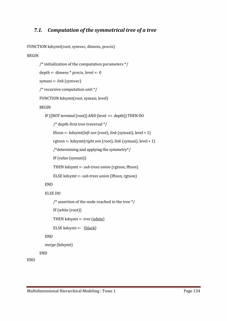
Multidimensional Hierarchical Modeling : Tome 1 Page 134
7.1. Computation of the symmetrical tree of a tree
FUNCTION kdsymt(root, symvec, dimens, precis)
BEGIN
/* initialization of the computation parameters */
depth <- dimens * precis, level <- 0
symaxi <- link (symvec)
/* recursive computation unit */
FUNCTION kdsymt(root, symaxi, level)
BEGIN
IF ((NOT terminal (root)) AND (level <> depth)) THEN DO
/* depth-first tree traversal */
lftson <- kdsymt(left son (root), link (symaxi), level + 1)
rgtson <- kdsymt(right son (root), link (symaxi), level + 1)
/*determining and applying the symmetry*/
IF (value (symaxi))
THEN kdsymt <- sub-trees union (rgtson, lftson)
ELSE kdsymt <- sub-trees union (lftson, rgtson)
END
ELSE DO
/* assertion of the node reached in the tree */
IF (white (root))
THEN kdsymt <- tree (white)
ELSE kdsymt <- (black)
END
merge (kdsymt)
END
END
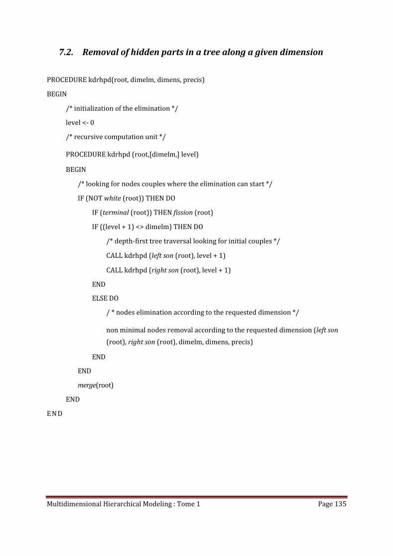
Multidimensional Hierarchical Modeling : Tome 1 Page 135
7.2. Removal of hidden parts in a tree along a given dimension
PROCEDURE kdrhpd(root, dimelm, dimens, precis)
BEGIN
/* initialization of the elimination */
level <- 0
/* recursive computation unit */
PROCEDURE kdrhpd (root,[dimelm,] level)
BEGIN
/* looking for nodes couples where the elimination can start */
IF (NOT white (root)) THEN DO
IF (terminal (root)) THEN fission (root)
IF ((level + 1) <> dimelm) THEN DO
/* depth-first tree traversal looking for initial couples */
CALL kdrhpd (left son (root), level + 1)
CALL kdrhpd (right son (root), level + 1)
END
ELSE DO
/ * nodes elimination according to the requested dimension */
non minimal nodes removal according to the requested dimension (left son
(root), right son (root), dimelm, dimens, precis)
END
END
merge(root)
END
EN D
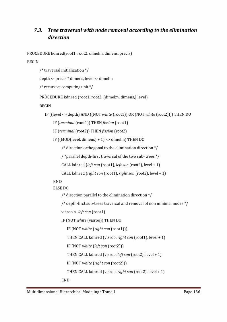
Multidimensional Hierarchical Modeling : Tome 1 Page 136
7.3. Tree traversal with node removal according to the elimination
direction
PROCEDURE kdnred(root1, root2, dimelm, dimens, precis)
BEGIN
/* traversal initialization */
depth <- precis * dimens, level <- dimelm
/* recursive computing unit */
PROCEDURE kdnred (root1, root2, [dimelm, dimens,] level)
BEGIN
IF ((level <> depth) AND ((NOT white (root1)) OR (NOT white (root2)))) THEN DO
IF (terminal (root1)) THEN fission (root1)
IF (terminal (root2)) THEN fission (root2)
IF ((MOD(level, dimens) + 1) <> dimelm) THEN DO
/* direction orthogonal to the elimination direction */
/ *parallel depth-first traversal of the two sub- trees */
CALL kdnred (left son (root1), left son (root2), level + 1)
CALL kdnred (right son (root1), right son (root2), level + 1)
END
ELSE DO
/* direction parallel to the elimination direction */
/* depth-first sub-trees traversal and removal of non minimal nodes */
visroo <- left son (root1)
IF (NOT white (visroo)) THEN DO
IF (NOT white (right son (root1)))
THEN CALL kdnred (visroo, right son (root1), level + 1)
IF (NOT white (left son (root2)))
THEN CALL kdnred (visroo, left son (root2), level + 1)
IF (NOT white (right son (root2)))
THEN CALL kdnred (visroo, right son (root2), level + 1)
END
Multidimensional Hierarchical Modeling : Tome 1 Page 137
visroo <- right son (root1)
IF (NOT white (visroo)) THEN DO
IF (NOT white (left son (root2)))
THEN CALL kdnred (visroo, left son (root2), level + 1)
IF (NOT white (right son (root2)))
THEN CALL kdnred (visroo, right son (root2), level + 1)
END
visroo <- left son (root2)
IF (NOT white (visroo)) THEN DO
IF (NOT white (right son (root2)))
THEN CALL kdnred (visroo, right son (root2), level + 1)
END
END
END
ELSE DO
/* removal of the hidden node */
IF (NOT white (root1)) THEN whiten (root2)
END
/* tree traversal return path */
merge(root1)
merge (root2)
END
END
Multidimensional Hierarchical Modeling : Tome 1 Page 138
7.4. Accumulation of planes orthogonal with the viewing axis in
order to perform a projection
FUNCTION kdplvi(root, dimvis, dimens ,precis)
BEGIN
/* projection initialization */
depth <- dimens * precis, level <- 0
/* recursive computing unit */
FUNCTION kdplvi(root,[dimvis, dimens,] level)
BEGIN
IF ((level <> depth) AND (NOT terminal (root))) THEN DO
/* depth-first traversal of the initial tree */
lftson <- kdplvi(left son (root), level + 1)
rgtson <- kdplvi(right son (root), level + 1)
/* projection computation */
IF ((MOD(level, dimens) + 1) = dimvis) THEN DO
/* projection according to the requested dimension*/
IF ((white (lftson) OR (white (rgtson)) THEN DO
IF ((white (lftson)) THEN DO
kdplvi <- rgtson
delete (lftson)
END
ELSE DO
kdplvi <- lftson
delete tree(rgtson)
END
END
Multidimensional Hierarchical Modeling : Tome 1 Page 139
ELSE DO
/* union of sub-trees */
kdplvi <- kdunio(lftson, rgtson, dimens, precis)
delete (lftson)
delete (rgtson)
END
END
ELSE sub-trees union (lftson, rgtson)
/* tree traversal return path */
merge(kdplvi)
END
ELSE DO
/*assertion of the node reached in the initial tree*/
IF (NOT white (root))
THEN kdplvi <- tree (black)
ELSE kdplvi <- tree (white)
END
END
END

Multidimensional Hierarchical Modeling : Tome 1 Page 140
Multidimensional Hierarchical Modeling : Tome 1 Page 141
8. Searching adjacencies
root : root of the tree to be processed
root1, root2 : symmetrical nodes in the tree
symmat : symmetry matrix
dimens : space dimension
precis : computation precision
depth : computation depth
level : level reached in the tree
symma2 : copy of the symmetry matrix
symvec : symmetry vector
symaxi : symmetry axis
remain : remainder of an Euclidean division
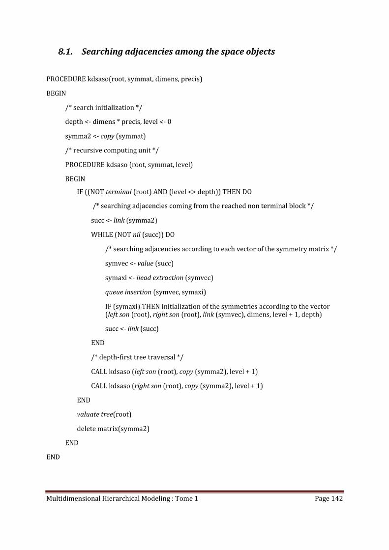
Multidimensional Hierarchical Modeling : Tome 1 Page 142
8.1. Searching adjacencies among the space objects
PROCEDURE kdsaso(root, symmat, dimens, precis)
BEGIN
/* search initialization */
depth <- dimens * precis, level <- 0
symma2 <- copy (symmat)
/* recursive computing unit */
PROCEDURE kdsaso (root, symmat, level)
BEGIN
IF ((NOT terminal (root) AND (level <> depth)) THEN DO
/* searching adjacencies coming from the reached non terminal block */
succ <- link (symma2)
WHILE (NOT nil (succ)) DO
/* searching adjacencies according to each vector of the symmetry matrix */
symvec <- value (succ)
symaxi <- head extraction (symvec)
queue insertion (symvec, symaxi)
IF (symaxi) THEN initialization of the symmetries according to the vector (left son (root), right son (root), link (symvec), dimens, level + 1, depth)
succ <- link (succ)
END
/* depth-first tree traversal */
CALL kdsaso (left son (root), copy (symma2), level + 1)
CALL kdsaso (right son (root), copy (symma2), level + 1)
END
valuate tree(root)
delete matrix(symma2)
END
END
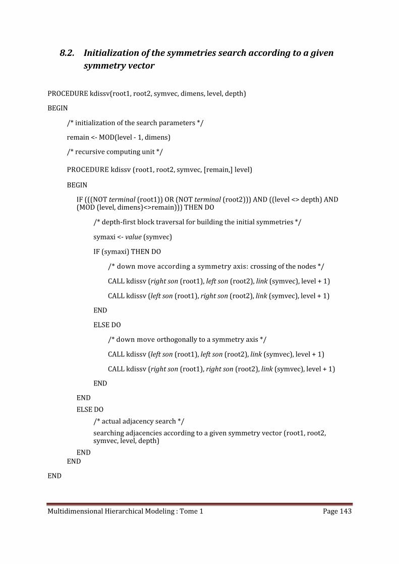
Multidimensional Hierarchical Modeling : Tome 1 Page 143
8.2. Initialization of the symmetries search according to a given
symmetry vector
PROCEDURE kdissv(root1, root2, symvec, dimens, level, depth)
BEGIN
/* initialization of the search parameters */
remain <- MOD(level - 1, dimens)
/* recursive computing unit */
PROCEDURE kdissv (root1, root2, symvec, [remain,] level)
BEGIN
IF (((NOT terminal (root1)) OR (NOT terminal (root2))) AND ((level <> depth) AND (MOD (level, dimens)<>remain))) THEN DO
/* depth-first block traversal for building the initial symmetries */
symaxi <- value (symvec)
IF (symaxi) THEN DO
/* down move according a symmetry axis: crossing of the nodes */
CALL kdissv (right son (root1), left son (root2), link (symvec), level + 1)
CALL kdissv (left son (root1), right son (root2), link (symvec), level + 1)
END
ELSE DO
/* down move orthogonally to a symmetry axis */
CALL kdissv (left son (root1), left son (root2), link (symvec), level + 1)
CALL kdissv (right son (root1), right son (root2), link (symvec), level + 1)
END
END
ELSE DO
/* actual adjacency search */
searching adjacencies according to a given symmetry vector (root1, root2, symvec, level, depth)
END
END
END
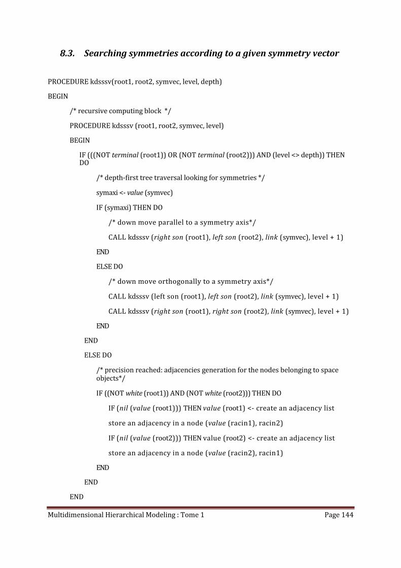
Multidimensional Hierarchical Modeling : Tome 1 Page 144
8.3. Searching symmetries according to a given symmetry vector
PROCEDURE kdsssv(root1, root2, symvec, level, depth)
BEGIN
/* recursive computing block */
PROCEDURE kdsssv (root1, root2, symvec, level)
BEGIN
IF (((NOT terminal (root1)) OR (NOT terminal (root2))) AND (level <> depth)) THEN DO
/* depth-first tree traversal looking for symmetries */
symaxi <- value (symvec)
IF (symaxi) THEN DO
/* down move parallel to a symmetry axis*/
CALL kdsssv (right son (root1), left son (root2), link (symvec), level + 1)
END
ELSE DO
/* down move orthogonally to a symmetry axis*/
CALL kdsssv (left son (root1), left son (root2), link (symvec), level + 1)
CALL kdsssv (right son (root1), right son (root2), link (symvec), level + 1)
END
END
ELSE DO
/* precision reached: adjacencies generation for the nodes belonging to space objects*/
IF ((NOT white (root1)) AND (NOT white (root2))) THEN DO
IF (nil (value (root1))) THEN value (root1) <- create an adjacency list
store an adjacency in a node (value (racin1), racin2)
IF (nil (value (root2))) THEN value (root2) <- create an adjacency list
store an adjacency in a node (value (racin2), racin1)
END
END
END

Multidimensional Hierarchical Modeling : Tome 1 Page 145
END

Multidimensional Hierarchical Modeling : Tome 1 Page 146

Multidimensional Hierarchical Modeling : Tome 1 Page 147
9. Tree labeling and extraction of segment trees
root : root of the labeled tree
adclls : list of the adjacency classes of the tree
bucket : bucket where are stored the adjacent nodes of a component
incpls list of the inside points of a component
adjque : queue of nodes adjacent to a current node
cncpnu : connected component number
cncomp : connected component
cptroo : root of a component tree (segment tree)
lftson : left son of a node
rgtson : right son of a node
9.1. Connected component labeling in a tree
FUNCTION kdcclb(root)
BEGIN
kdcclb <-- create list of connected components
search of adjacency classes (root, kdcclb)
tree labeling (kdcclb)
END
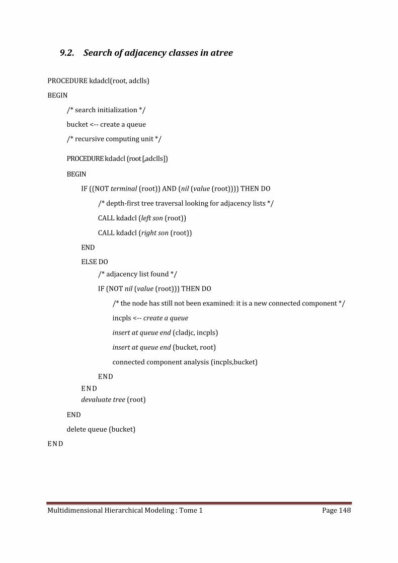
Multidimensional Hierarchical Modeling : Tome 1 Page 148
9.2. Search of adjacency classes in atree
PROCEDURE kdadcl(root, adclls)
BEGIN
/* search initialization */
bucket <-- create a queue
/* recursive computing unit */
PROCEDURE kdadcl (root [,adclls])
BEGIN
IF ((NOT terminal (root)) AND (nil (value (root)))) THEN DO
/* depth-first tree traversal looking for adjacency lists */
CALL kdadcl (left son (root))
CALL kdadcl (right son (root))
END
ELSE DO
/* adjacency list found */
IF (NOT nil (value (root))) THEN DO
/* the node has still not been examined: it is a new connected component */
incpls <-- create a queue
insert at queue end (cladjc, incpls)
insert at queue end (bucket, root)
connected component analysis (incpls,bucket)
END
E N D
devaluate tree (root)
END
delete queue (bucket)
EN D
Multidimensional Hierarchical Modeling : Tome 1 Page 149
9.3. Connected component analysis
PROCEDURE kdccan(incpls, bucket)
BEGIN
/* process adjacent nodes of the bucket until running out */
WHILE (NOT empty (bucket)) DO
/* move a node from the bucket into the connected component */
root <-- extract from queue head (bucket)
IF (NOT nil (value (root))) THEN insert at queue end (incpls, root)
/* scrutation des voisins du nœud transféré */
filadj <-- value (root)
WHILE (NOT empty (adjque)) DO
/* its neighbors are poured in the bucket */
insert at queue end (bucket, extract from queue head (adjque))
END
delete queue(adjque)
END
EN D

Multidimensional Hierarchical Modeling : Tome 1 Page 150
9.4. Labeling a tree
PROCEDURE kdtlab(adclls)
BEGIN
/* scrutinizing connected components registered in the adjacency class list */
cncpnu <-- 0
cncomp <-- link (adclls)
WHILE (NOT nil (cncomp)) DO
cncpnu <-- cncpnu + 1
incpls <-- value (cncomp)
/* labeling of the inside of the connected component */
WHILE (NOT empty (incpls)) DO
root <-- extract from queue head (incpls)
value (root) <-- cncpnu
END
delete queue (incpls)
erase its references in the structure (cncomp)
cncomp <-- link (cncomp)
E N D
EN D
Multidimensional Hierarchical Modeling : Tome 1 Page 151
9.5. Building the segment trees from the connected components of a
labeled tree
PROCEDURE kdbsgt(cladjc,racine)
BEGIN
/* scrutinizing the connected components registered in the adjacency class list */
cncpnu <-- 0
cncomp <-- link (adclls)
WHILE (NOT nil (cncomp)) DO
/* building the tree of the current connected component */
cncpnu <-- cncpnu + 1
cptroo <-- extraction of a connected component from a tree (root, cncpnu)
/* hanging of the segment tree in the adjacency class list */
value (cncomp) <-- cptroo
EN D
E N D
Multidimensional Hierarchical Modeling : Tome 1 Page 152
9.6. Extraction of a connected component from a tree
FUNCTION kdexcc(root, cncomp)
BEGIN
/* recursive computing unit */
FUNCTION kdexcc(root [ ,cncomp])
BEGIN
IF ((NOT terminal (root)) AND (nil (value (root))))
THEN DO
/* depth-first tree traversal searching labeled nodes */
lftson <-- kdexcc (left son (root))
rgtson <-- kdexcc (right son (root))
kdexcc <-- sub-trees union (lftson, rgtson)
END
ELSE DO
/*create a black node when the node label is corresponding to the searched component*/
IF (value (root) = cncomp)
THEN kdexcc <-- tree (black)
ELSE kdexcc <-- tree (white)
END
/* tree traversal return path */
IF ((NOT terminal (kdexcc)) THEN merge (kdexcc)
EN D
E N D

Multidimensional Hierarchical Modeling : Tome 1 Page 153
10. Computation of the generalized moment list of a tree
root : root of the tree
dimens : dimension of the modeling space
precis : computation precision
depth : computation depth
level : level reached in the tree
minroo : minimum coordinates list of the root
maxroo : maximum coordinates list of the root
{ minson, maxson} : min. et max. coordinates list of a son
nudim : coordinate number
{nudim1, nudim2, nudim3} : coordinate numbers
{x1 , x2, x3} : simple, squared, cubic value of a coordinate
x : coordinate
ncoord : number of the block dividing coordinate
moment : moment list
index : computation or table index
momroo: moment list of the root
{momlft, momrgt} : moment lists of left and right sons
Multidimensional Hierarchical Modeling : Tome 1 Page 154
10.1. Computation of the moment list of a tree
FUNCTION kdmomt (root, dimens, precis)
BEGIN
/* moments computation initialization */
{minroo, maxroo} <-- vector {(0., 0., ..., 0.),(1.,1., ..., 1.)}
momroo<-- moment list of the unitary space (dimens)
value(root) <-- momroo
depth <-- precis * dimens, level <-- 0
/* recursive computing unit */
PROCEDURE kdmomt (root, minroo, maxroo, level)
BEGIN
IF ((NOT terminal (root)) AND (level <> depth)) THEN DO
/* computation of the left node moments */
minson <-- copy (minroo), maxson <-- copy (maxroo)
nudim <-- MOD(level, dimens) + 1
momroo<-- value (root)
value (left son (root)) <-- child moment list computation (momroo, nudim, minroo(nudim), dimens)
maxson(nudim) <-- (minroo(nudim) + maxroo(nudim))/2.
CALL kdmomt (left son (root), minson, maxson, level + 1)
/* computation of the right node moments */
minson <-- copy (minroo), maxson <-- copy (maxroo)
nudim <-- MOD(level, dimens) + 1
momroo<-- value (root)
value (right son (root)) <-- child moment list computation (momroo, nudim, maxroo(nudim), dimens)
minson(nudim) <-- (minroo(nudim) + maxroo(nudim))/2.
CALL kdmomt (right son (root), minson, maxson, level + 1)
/* evaluation of the tree moments on return path */
cumulative children moments (root)

Multidimensional Hierarchical Modeling : Tome 1 Page 155
END
END
/* moment list retrieval */
kdmomt <-- value (root)
value(root) <-- nil
END
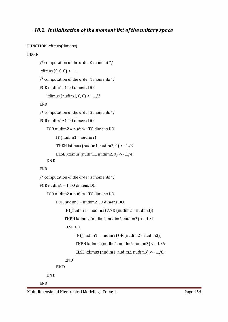
Multidimensional Hierarchical Modeling : Tome 1 Page 156
10.2. Initialization of the moment list of the unitary space
FUNCTION kdimus(dimens)
BEGIN
/* computation of the order 0 moment */
kdimus (0, 0, 0) <-- 1.
/* computation of the order 1 moments */
FOR nudim1=1 TO dimens DO
kdimus (nudim1, 0, 0) <-- 1./2.
END
/* computation of the order 2 moments */
FOR nudim1=1 TO dimens DO
FOR nudim2 = nudim1 TO dimens DO
IF (nudim1 = nudim2)
THEN kdimus (nudim1, nudim2, 0) <-- 1./3.
ELSE kdimus (nudim1, nudim2, 0) <-- 1./4.
EN D
END
/* computation of the order 3 moments */
FOR nudim1 = 1 TO dimens DO
FOR nudim2 = nudim1 TO dimens DO
FOR nudim3 = nudim2 TO dimens DO
IF ((nudim1 = nudim2) AND (nudim2 = nudim3))
THEN kdimus (nudim1, nudim2, nudim3) <-- 1./4.
ELSE DO
IF ((nudim1 = nudim2) OR (nudim2 = nudim3))
THEN kdimus (nudim1, nudim2, nudim3) <-- 1./6.
ELSE kdimus (nudim1, nudim2, nudim3) <-- 1./8.
END
END
EN D
END
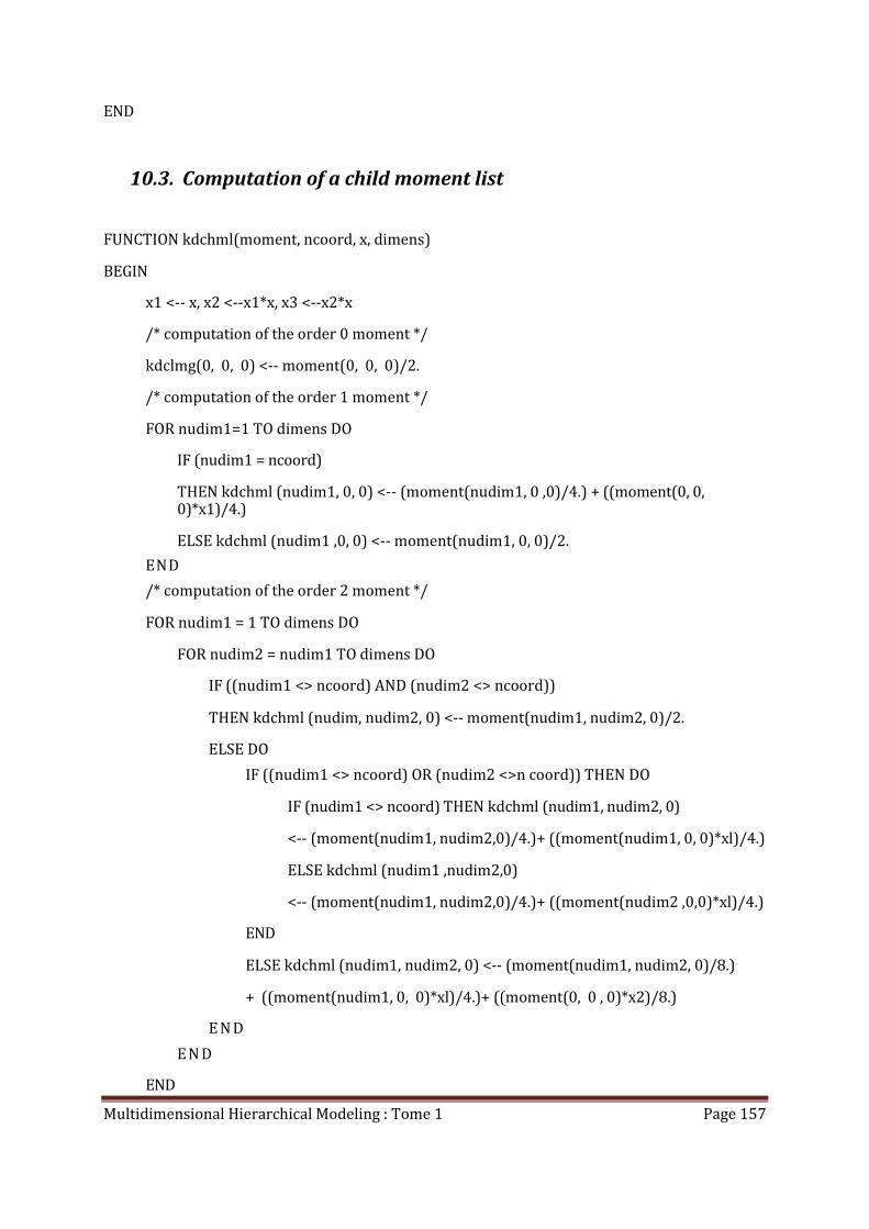
Multidimensional Hierarchical Modeling : Tome 1 Page 157
END
10.3. Computation of a child moment list
FUNCTION kdchml(moment, ncoord, x, dimens)
BEGIN
x1 <-- x, x2 <--x1*x, x3 <--x2*x
/* computation of the order 0 moment */
kdclmg(0, 0, 0) <-- moment(0, 0, 0)/2.
/* computation of the order 1 moment */
FOR nudim1=1 TO dimens DO
IF (nudim1 = ncoord)
THEN kdchml (nudim1, 0, 0) <-- (moment(nudim1, 0 ,0)/4.) + ((moment(0, 0, 0)*x1)/4.)
ELSE kdchml (nudim1 ,0, 0) <-- moment(nudim1, 0, 0)/2.
END
/* computation of the order 2 moment */
FOR nudim1 = 1 TO dimens DO
FOR nudim2 = nudim1 TO dimens DO
IF ((nudim1 <> ncoord) AND (nudim2 <> ncoord))
THEN kdchml (nudim, nudim2, 0) <-- moment(nudim1, nudim2, 0)/2.
ELSE DO
IF ((nudim1 <> ncoord) OR (nudim2 <>n coord)) THEN DO
IF (nudim1 <> ncoord) THEN kdchml (nudim1, nudim2, 0)
<-- (moment(nudim1, nudim2,0)/4.)+ ((moment(nudim1, 0, 0)*xl)/4.)
ELSE kdchml (nudim1 ,nudim2,0)
<-- (moment(nudim1, nudim2,0)/4.)+ ((moment(nudim2 ,0,0)*xl)/4.)
END
ELSE kdchml (nudim1, nudim2, 0) <-- (moment(nudim1, nudim2, 0)/8.)
+ ((moment(nudim1, 0, 0)*xl)/4.)+ ((moment(0, 0 , 0)*x2)/8.)
E N D
E N D
END
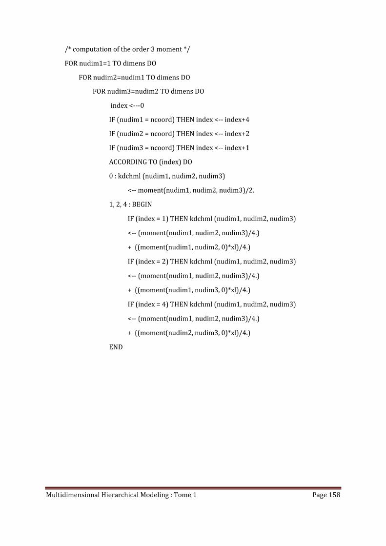
Multidimensional Hierarchical Modeling : Tome 1 Page 158
/* computation of the order 3 moment */
FOR nudim1=1 TO dimens DO
FOR nudim2=nudim1 TO dimens DO
FOR nudim3=nudim2 TO dimens DO
index <---0
IF (nudim1 = ncoord) THEN index <-- index+4
IF (nudim2 = ncoord) THEN index <-- index+2
IF (nudim3 = ncoord) THEN index <-- index+1
ACCORDING TO (index) DO
0 : kdchml (nudim1, nudim2, nudim3)
<-- moment(nudim1, nudim2, nudim3)/2.
1, 2, 4 : BEGIN
IF (index = 1) THEN kdchml (nudim1, nudim2, nudim3)
<-- (moment(nudim1, nudim2, nudim3)/4.)
+ ((moment(nudim1, nudim2, 0)*xl)/4.)
IF (index = 2) THEN kdchml (nudim1, nudim2, nudim3)
<-- (moment(nudim1, nudim2, nudim3)/4.)
+ ((moment(nudim1, nudim3, 0)*xl)/4.)
IF (index = 4) THEN kdchml (nudim1, nudim2, nudim3)
<-- (moment(nudim1, nudim2, nudim3)/4.)
+ ((moment(nudim2, nudim3, 0)*xl)/4.)
END
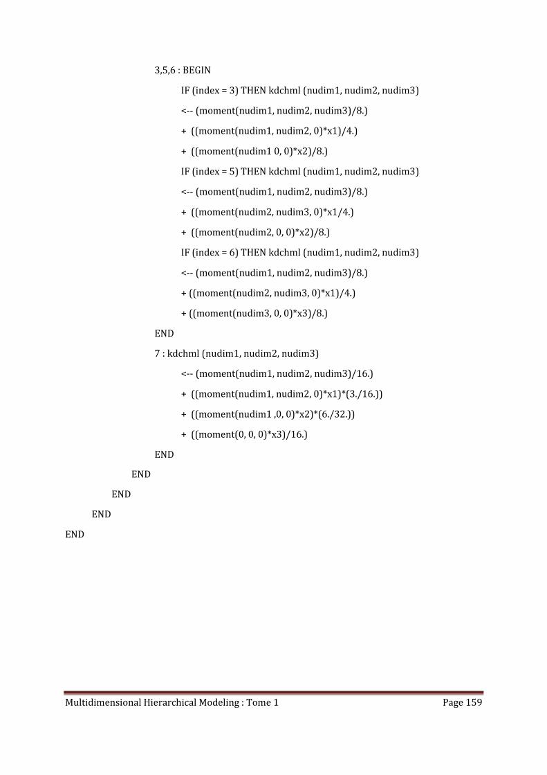
Multidimensional Hierarchical Modeling : Tome 1 Page 159
3,5,6 : BEGIN
IF (index = 3) THEN kdchml (nudim1, nudim2, nudim3)
<-- (moment(nudim1, nudim2, nudim3)/8.)
+ ((moment(nudim1, nudim2, 0)*x1)/4.)
+ ((moment(nudim1 0, 0)*x2)/8.)
IF (index = 5) THEN kdchml (nudim1, nudim2, nudim3)
<-- (moment(nudim1, nudim2, nudim3)/8.)
+ ((moment(nudim2, nudim3, 0)*x1/4.)
+ ((moment(nudim2, 0, 0)*x2)/8.)
IF (index = 6) THEN kdchml (nudim1, nudim2, nudim3)
<-- (moment(nudim1, nudim2, nudim3)/8.)
+ ((moment(nudim2, nudim3, 0)*x1)/4.)
+ ((moment(nudim3, 0, 0)*x3)/8.)
END
7 : kdchml (nudim1, nudim2, nudim3)
<-- (moment(nudim1, nudim2, nudim3)/16.)
+ ((moment(nudim1, nudim2, 0)*x1)*(3./16.))
+ ((moment(nudim1 ,0, 0)*x2)*(6./32.))
+ ((moment(0, 0, 0)*x3)/16.)
END
END
END
END
END

Multidimensional Hierarchical Modeling : Tome 1 Page 160
10.4. Cumulative node children moments
PROCEDURE kdcucm(root)
BEGIN
/* retrieval of father and children moment lists */
momroo <-- value (root)
momlft<-- value (left son (root))
momrgt <-- value (right son (root))
/* scrutinizing of the three lists and cumulative children moments into father’s ones */
FOR index = 0 TO (C1dimens + C2
dimens + C3dimens) DO
IF (white (left son (root))) THEN momlft(index) <-- O.
IF (white (right son (root))) THEN monrgt(index) <-- O.
momroo(index) <-- momlft(index) + momrgt(index)
END
/* devaluation of the children nodes */
delete list (momlft)
delete list (momrgt)
value (left son (root)) <-- nil
value (right son (root)) <-- nil
END
Multidimensional Hierarchical Modeling : Tome 1 Page 161
11. Centering and normalizing a generalized moments
list
moment : moment list to be processed
momnor : normalized moment list
matrot : generalized rotation matrix in homogenous coordinates
dimens : dimension of the modeling space
nudim : coordinate number
nudim1 : first coordinate number
nudim2 : second coordinate number
nudim3 : third coordinate number
vectr : vector of the gravity center
hypvol : tree hypervolume
matsym : inertia matrix extracted from the moment list
matvpr : matrix of Eigen vectors of the tree Eigen reference frame
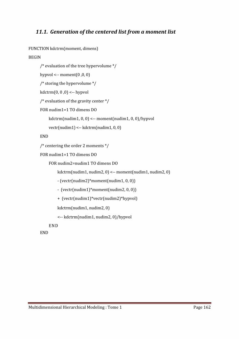
Multidimensional Hierarchical Modeling : Tome 1 Page 162
11.1. Generation of the centered list from a moment list
FUNCTION kdctrm(moment, dimens)
BEGIN
/* evaluation of the tree hypervolume */
hypvol <-- moment(0 ,0, 0)
/* storing the hypervolume */
kdctrm(0, 0 ,0) <-- hypvol
/* evaluation of the gravity center */
FOR nudim1=1 TO dimens DO
kdctrm(nudim1, 0, 0) <-- moment(nudim1, 0, 0)/hypvol
vectr(nudim1) <-- kdctrm(nudim1, 0, 0)
END
/* centering the order 2 moments */
FOR nudim1=1 TO dimens DO
FOR nudim2=nudim1 TO dimens DO
kdctrm(nudim1, nudim2, 0) <-- moment(nudim1, nudim2, 0)
- (vectr(nudim2)*moment(nudim1, 0, 0))
- (vectr(nudim1)*moment(nudim2, 0, 0))
+ (vectr(nudim1)*vectr(nudim2)*hypvol)
kdctrm(nudim1, nudim2, 0)
<-- kdctrm(nudim1, nudim2, 0)/hypvol
END
END
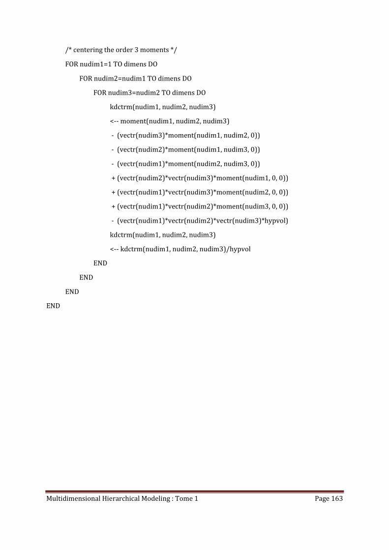
Multidimensional Hierarchical Modeling : Tome 1 Page 163
/* centering the order 3 moments */
FOR nudim1=1 TO dimens DO
FOR nudim2=nudim1 TO dimens DO
FOR nudim3=nudim2 TO dimens DO
kdctrm(nudim1, nudim2, nudim3)
<-- moment(nudim1, nudim2, nudim3)
- (vectr(nudim3)*moment(nudim1, nudim2, 0))
- (vectr(nudim2)*moment(nudim1, nudim3, 0))
- (vectr(nudim1)*moment(nudim2, nudim3, 0))
+ (vectr(nudim2)*vectr(nudim3)*moment(nudim1, 0, 0))
+ (vectr(nudim1)*vectr(nudim3)*moment(nudim2, 0, 0))
+ (vectr(nudim1)*vectr(nudim2)*moment(nudim3, 0, 0))
- (vectr(nudim1)*vectr(nudim2)*vectr(nudim3)*hypvol)
kdctrm(nudim1, nudim2, nudim3)
<-- kdctrm(nudim1, nudim2, nudim3)/hypvol
END
END
END
END

Multidimensional Hierarchical Modeling : Tome 1 Page 164
11.2. Generation of the moment normalized list and the rotation
matrix
PROCEDURE kdnrmr(moment, momnor, matrot, dimens)
BEGIN
/* copying out volume and gravity center coordinates*/
momnor(0, 0, 0) <-- moment(0, 0, 0)
FOR nudim1=1 TO dimens DO
momnor(nudim1, 0, 0) <-- moment(nudim1, 0, 0)
END
/* building and diagonalization of the inertia matrix */
FOR nudim1=1 TO dimens DO
FOR nudim2=nudim1 TO dimens DO
matsym(nudim1, nudim2) <-- moment(nudim1, nudim2, 0)
END
END
compute Eigen values and vectors (matsym, matvpr, dimens)
/* inertia axes computation */
FOR nudim=1 TO dimens DO
momnor(nudim, nudim, 0) <-- matsym(nudim, nudim)
END
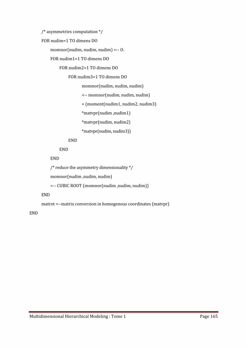
Multidimensional Hierarchical Modeling : Tome 1 Page 165
/* asymmetries computation */
FOR nudim=1 TO dimens DO
momnor(nudim, nudim, nudim) <-- O.
FOR nudim1=1 TO dimens DO
FOR nudim2=1 TO dimens DO
FOR nudim3=1 TO dimens DO
momnor(nudim, nudim, nudim)
<-- momnor(nudim, nudim, nudim)
+ (moment(nudim1, nudim2, nudim3)
*matvpr(nudim ,nudim1)
*matvpr(nudim, nudim2)
*matvpr(nudim, nudim3))
END
END
END
/* reduce the asymmetry dimensionality */
momnor(nudim ,nudim, nudim)
<-- CUBIC ROOT (momnor(nudim ,nudim, nudim))
END
matrot <--matrix conversion in homogenous coordinates (matvpr)
END

Multidimensional Hierarchical Modeling : Tome 1 Page 166
11.3. Generation of the moment normalized list
FUNCTION kdnrmg(moment, dimens)
This function is analogous to kdnrmr, except that:
− the generalized rotation matrix is not retrieved;
− the uncertainty about the directions of Eigen axes is removed giving back positive
asymmetries.
Multidimensional Hierarchical Modeling : Tome 1 Page 167
12. Generation of an Eigen tree
root : root of the tree to be transformed
momnor : tree centered and reduced moment list
matrot : rotation matrix associated to the Eigen reference frame
dimens : dimension of the modeled space
prec1 : analysis precision
prec2 : computation precision
nudim : coordinate number
vect : work vector
{mdtr, mitr } direct and inverse translation matrices
{mdan, mian} : direct and inverse homothety matrices
{mdcr, micr} : direct and inverse rotation centering matrices
mirt : inverse rotation matrices
{mart ,mtra} : direct and inverse transformation matrices
{polesp, minesp, maxesp} : unitary space polyhedron
{ polyed, minhyp, maxhyp} : transformation polyhedron
homotr : homogenous transformed tree
tabsym : table of symmetries (signature of the Eigen reference frame)
vecsym : symmetry vector
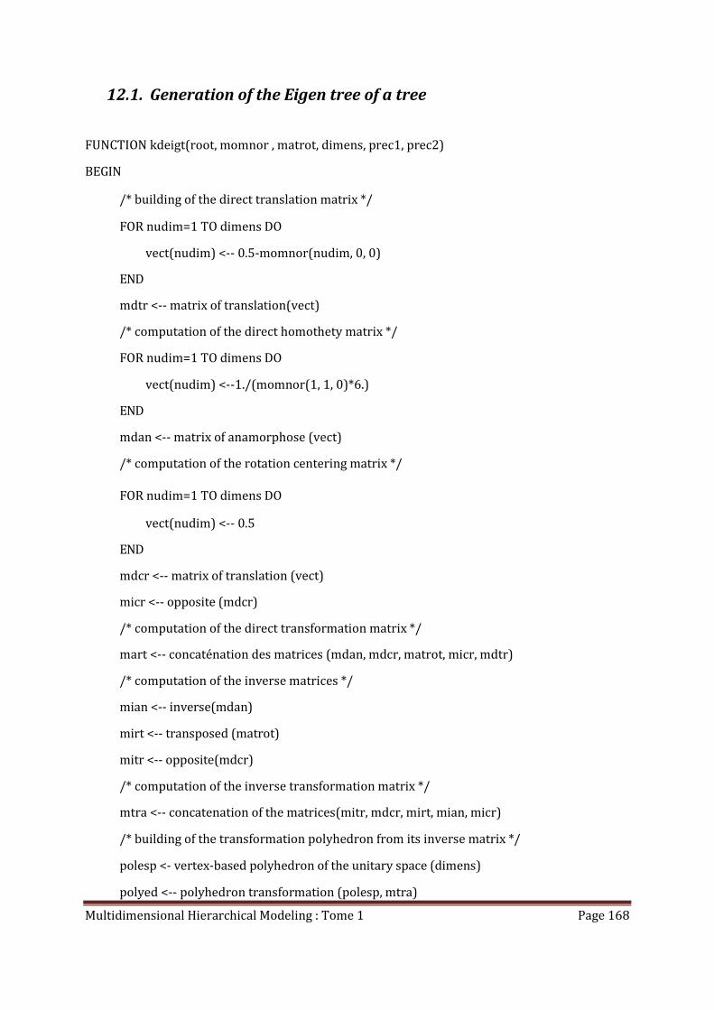
Multidimensional Hierarchical Modeling : Tome 1 Page 168
12.1. Generation of the Eigen tree of a tree
FUNCTION kdeigt(root, momnor , matrot, dimens, prec1, prec2)
BEGIN
/* building of the direct translation matrix */
FOR nudim=1 TO dimens DO
vect(nudim) <-- 0.5-momnor(nudim, 0, 0)
END
mdtr <-- matrix of translation(vect)
/* computation of the direct homothety matrix */
FOR nudim=1 TO dimens DO
vect(nudim) <--1./(momnor(1, 1, 0)*6.)
END
mdan <-- matrix of anamorphose (vect)
/* computation of the rotation centering matrix */
FOR nudim=1 TO dimens DO
vect(nudim) <-- 0.5
END
mdcr <-- matrix of translation (vect)
micr <-- opposite (mdcr)
/* computation of the direct transformation matrix */
mart <-- concaténation des matrices (mdan, mdcr, matrot, micr, mdtr)
/* computation of the inverse matrices */
mian <-- inverse(mdan)
mirt <-- transposed (matrot)
mitr <-- opposite(mdcr)
/* computation of the inverse transformation matrix */
mtra <-- concatenation of the matrices(mitr, mdcr, mirt, mian, micr)
/* building of the transformation polyhedron from its inverse matrix */
polesp <- vertex-based polyhedron of the unitary space (dimens)
polyed <-- polyhedron transformation (polesp, mtra)
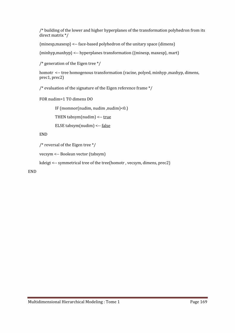
Multidimensional Hierarchical Modeling : Tome 1 Page 169
/* building of the lower and higher hyperplanes of the transformation polyhedron from its direct matrix */
{minesp,maxesp} <-- face-based polyhedron of the unitary space (dimens)
{minhyp,maxhyp} <-- hyperplanes transformation ({minesp, maxesp}, mart)
/* generation of the Eigen tree */
homotr <-- tree homogenous transformation (racine, polyed, minhyp ,maxhyp, dimens, prec1, prec2)
/* evaluation of the signature of the Eigen reference frame */
FOR nudim=1 TO dimens DO
IF (momnor(nudim, nudim ,nudim)<0.)
THEN tabsym(nudim) <-- true
ELSE tabsym(nudim) <-- false
END
/* reversal of the Eigen tree */
vecsym <-- Boolean vector (tabsym)
kdeigt <-- symmetrical tree of the tree(homotr , vecsym, dimens, prec2)
END

Multidimensional Hierarchical Modeling : Tome 1 Page 170
12.2. Generation of the Eigen tree of a tree (fast version)
FUNCTION kdfeit(root, momnor, matrot, dimens, precl, prec2)
This function is analogous to kdeigt, except that:
- the tree homogenous transform is replaced by its fast version.