hierarchical phrase-based translation with weighted finite-state
TRANSCRIPT

Hierarchical Phrase-based
Translation with Weighted
Finite-State Transducers
Universidade de Vigo
Departamento de Teoría do Sinal e Comunicacións
AuthorGonzalo Iglesias
AdvisorsAdrià de Gispert
Eduardo R. Banga
2010“DOCTOR EUROPEUS”


Departamento de Teoría do Sinal e ComunicaciónsUniversidade de Vigo
SPAIN
Ph.D Thesis Dissertation
Hierarchical Phrase-based Translationwith Weighted Finite-State Transducers
Author: Gonzalo Iglesias
Advisors: Adrià de GispertEduardo R. Banga
January 2010


TESIS DOCTORAL
Hierarchical Phrase-based Translationwith Weighted Finite-State Transducers
Autor: Gonzalo IglesiasDirectores:Adrià de Gispert
Eduardo R. Banga
TRIBUNAL CALIFICADOR
Presidente: Dr. D.
Vocales:
Dr. D.
Dr. D.
Dr. D.
Secretario: Dr. D.
CALIFICACIÓN:
Vigo, a de de .


“An idle mind is the Devil’s seedbed”
Tad Williams


Esta tesis se la dedico a mis padres y a Aldara.


Acknowledgements
This work has been supported by Spanish Government researchgrantBES-2007-15956, project AVIVAVOZ (TEC2006-13694-C03-03) and projectBUCEADOR (TEC2009-14094-C04-04). Also supported in part by the GALE pro-gram of the Defense Advanced Research Projects Agency, Contract No. HR0011-06-C-0022.


Abstract
This dissertation is focused in the Statistical Machine Translation field (SMT),
particularly in hierarchical phrase-based translation frameworks. We first study and
redesign hierarchical models using several filtering techniques. Hierarchical search
spaces are based on automatically extracted translation rules. As originally defined
they are too big to handle directly without filtering. In thisthesis we create more
space-efficient models, aiming at faster decoding times without a cost in perfor-
mance. We propose more refined strategies such as pattern filtering and shallow-n
grammars. The aim is to reduce a priori the search space as much as possible without
losing performance (or even improving it), so that search errors will be avoided.
We also propose a new algorithm in the hierarchical phrase-based machine
translation framework, calledHiFST. For the first time, as far as we are aware,
an SMT system combines successfully knowledge from two other research
areas simultaneously:parsing, and weighted finite-state technology. In this way
we are able to build a more efficient decoding tool, taking theadvantages of
both worlds: the capability of deep syntax reordering with parsing, and the
compact representation and powerful semiring operations of weighted finite-
state transducers. Combined with our findings for hierarchical grammars, we are
able to build search-error free translation systems with state-of-the-art performance.
Keywords: HiFST, SMT, hierarchical phrase-based decoding, parsing,CYK,
WFSTs, transducers.


Resumen
Objetivos
Esta tesis se centra en dos objetivos relacionados con el conocido problema
computacional de la búsqueda, en el marco de la traducción defrases jerárquicas.
Por un lado, queremos definir un espacio de hipótesis lo más compacto y completo
posible; por el otro, procuramos un nuevo algoritmo que ejecute la búsqueda sobre
dicho espacio de la forma más eficiente posible.
Los sistemas de traducción de frases jerárquicas[Chiang, 2007] utilizan
gramáticas incontextuales síncronas que se inducen automáticamente a partir de un
corpus bilingüe de texto, sin conocimiento lingüístico previo. La idea subyacente
es que los dos idiomas pueden representarse con una estructura sintáctica común,
lo que permite un sistema de traducción con gran capacidad para realizar reorde-
namientos de palabras a larga distancia.
Es importante destacar que dicha gramática define el espaciode hipótesis en el
que estaremos buscando nuestra traducción. En consecuencia, modelamos indirec-
tamente el espacio de hipótesis elaborando estrategias querefinen adecuadamente
la gramática. Una vez tenemos esta gramática preparada, se utiliza un analizador
para obtener, dada una oración del lenguaje fuente, un conjunto de posibles análisis
sintácticos representados como secuencias de reglas oderivaciones. Usando esta
información, es posible construir listas de hipótesis de traducción con sus respec-
tivos costes. Esta organización en listas de hipótesis constituye una limitación habi-
tual de los decodificadores jerárquicos. Como demostraremos a lo largo de la di-
sertación, resulta más eficiente utilizar representaciones más compactas, como son
lascelosías. A continuación, describimos los objetivos de esta tesis:

IV
1. Proponemos un nuevo algoritmo de traducción de frases jerárquicas, llama-
do HiFST. Esta herramienta utiliza los conocimientos de tres áreas de in-
vestigación:análisis sintáctico, máquinas de estados finitosy, por supuesto,
traducción automática. Existen bastantes aportaciones previas en el campo
de traducción estadística con máquinas de estados finitos, por una parte; y
con algoritmos de análisis sintáctico, por la otra. Pero porprimera vez, que
sepamos, un sistema de traducción automática combina la capacidad de re-
ordenamiento de los algoritmos de análisis sintáctico con la representación
compacta y eficiente de celosías implementadas mediante transductores que
permiten el uso sencillo de operaciones complejas como minimización, deter-
minización, composición, etc.
2. Refinamos los modelos jerárquicos utilizando varias técnicas de filtrado. Los
espacios de búsqueda se basan en reglas jerárquicas de traducción extraí-
das automáticamente. La gramática inicial es demasiado grande como para
utilizar directamente sin filtrar. En esta tesis vamos a buscar modelos más
eficientes, con vistas a tiempos más rápidos de decodificación sin pérdida
de calidad. En concreto, en vez del filtrado habitual por número mínimo de
instancias de reglas extraídas del corpus de entrenamiento(mincount), pro-
ponemos estrategias más refinadas, como el filtrado de patrones y las gramáti-
casshallow-N . El objetivo es reducir a priori el espacio de búsqueda lo más
posible sin perder calidad (o incluso mejorando), para evitar los errores de
búsqueda derivados de podas en modelos durante su proceso deconstrucción.
En resumen, estos objetivos pueden englobarse en uno único yambicioso: la
construcción de un sistema que traduzca con la mayor calidadposible, capaz de
alcanzar el estado del arte, incluso para tareas de traducción a gran escala, que
requieren de enormes cantidades de datos.
Organización de la Tesis
A continuación exponemos la estructura de la tesis:
En el Capítulo 1 motivamos e introducimos esta disertación.
En el Capítulo 2 sentamos las bases deHiFST. Se introducen los transduc-
tores de estados finitos, y explicamos mediante ejemplos diversas operaciones

V
posibles (unión, concatenación, composición, ...). También describimos el al-
goritmo CYK y realizamos una revisión histórica del análisis sintáctico como
problema computacional.
El Capítulo 3 se dedica a la traducción estadística. Despuésde una introduc-
ción histórica se describen los conceptos fundamentales para el estado del arte
de la traducción estadística, tal como la entendemos hoy en día.
Ya en el Capítulo 4 centramos esta disertación en los sistemas de traduc-
ción jerárquica. Específicamente se describen los detallesde implementación
de un decodificador de poda hipercúbica (HCP) y proponemos mejoras a la
aplicación estándar. También describimos unos cuantos experimentos de con-
traste con otro traductor basado en frases, del que derivamos conclusiones
importantes para el espacio de búsqueda jerárquica en el capítulo siguiente.
Este capítulo termina con una revisión de las aportaciones más importantes
durante estos años al campo de la traducción estadística de frases jerárquicas.
El Capítulo 5 se concentra en la creación eficiente de espacios de búsqueda
definidos a través de las gramáticas jerárquicas. Se introducen los patrones
como un concepto clave para aplicar filtrados selectivos. Mostramos cómo
construir estas gramáticas combinando diversas técnicas de filtrado. Además,
introducimos nuevas variantes como la familia de gramáticasshallow-N . Eva-
luamos nuestro método con una serie de experimentos para la tarea de traduc-
ción de árabe a inglés.
En el Capítulo 6 presentamosHiFST. Se explican en detalle los algoritmos
de traducción, que utilizan transductores. Describimos dos métodos de ali-
neación para el proceso de optimización. Evaluamos nuestrotraductor con
una batería de experimentos para tres tareas de traducción,empezando con
un contraste entreHiFST y HCP para árabe-inglés y chino-inglés. También
incluimos experimentos conHiFST para gramáticasshallow-N , descritas en
el capítulo anterior.
El Capítulo 7 extrae las conclusiones más importantes de la tesis y propone
varias líneas futuras.
A continuación describimos con más detalle esta tesis. En primer lugar expli-
caremos la traducción basada en frases jerárquicas. Luego plantearemos algunas es-

VI
trategias para filtrar gramáticas; finalmente expondremos los detalles más relevantes
de nuestro nuevo sistema de traducción, denominadoHiFST.
Traducción basada en Frases Jerárquicas
Gramáticas Síncronas
El problema de la traducción estadística basada en frases semodela como una
gramática incontextual síncrona, que es simplemente un conjunto R = Rr de
reglasRr : N → 〈γr,αr〉 / pr, dondepr es la probabilidad de esta regla síncrona y
γ, α ∈ (N ∪ T)∗ son las frases (secuencias de terminales y no terminales) para la
lengua origen y la frase en la lengua destino, respectivamente.N ∈ N es cualquier
no terminal (constituyente o categoría).
gramática estándar jerárquicaS→〈X,X〉 regla ‘glue’ 1S→〈S X,S X〉 regla ‘glue’ 2X→〈γ,α,∼〉 , γ, α ∈ X ∪T+ reglas jerárquicas
Cuadro 1: Reglas de una gramática estándar jerárquica.T es el conjunto de termi-nales (palabras).
Más específicamente, el Cuadro 1 resume el tipo de reglas utilizadas por una
gramática jerárquica. Solo se admiten dos no terminalesS oX, constituyentes abs-
tractos, es decir, sin ningún significado sintáctico. La gramática incluye un par de
reglas especiales llamadas reglas ‘glue’[Chiang, 2007], que permiten la concate-
nación de las frases jerárquicas. Cada regla de cabeceraX nos indica que la frase
jerárquicaα es la traducción deγ (con una cierta probabilidad). Las reglas con
cabeceraX pueden a su vez incorporar en el cuerpo un número arbitrario de no
terminalesX, que se pueden traducir en cualquier orden. Siempre ha de existir el
mismo número deX para la frase origen que para la frase destino. La forma en que
se reordenan los no terminales se establece formalmente mediante∼, una función
biyectiva que relaciona los no terminales del la frase de lengua origen y los no termi-
nales de la frase de lengua destino de cada regla. Para reglasconcretas,∼ no se usa;
en su lugar, los no terminales llevan un subíndice que marcanla correspondencia,
como puede verse en la siguiente regla jerárquica con dos no terminales:
X → 〈 X2 en X1 ocasiones , on X1 occasions X2〉

VII
Cuando para una regla se cumple queγ, α ∈ T+, es decir, que no existe ningún
no terminal en la regla, entonces estamos ante una frase puramente léxica, que cons-
tituye el núcleo de cualquier sistema de traducción basado en frases.
Las reglas se extraen a partir de un corpus paralelo de textosen ambos idiomas
de interés. Dicha extracción se aplica con una serie de restricciones, como por ejem-
plo que no se permiten más de dos no terminales en una frase jerárquica. El heurís-
tico se describe con más detalle en la Sección 4.2. Las probabilidades de las frases
jerárquicas se obtienen contando el número de apariciones relativas en el corpus de
entrenamiento como se indica en la Sección 3.5.
Decodificador de Poda Hipercúbica
Figura 1: Decodificador de poda hipercúbica (HCP).
El decodificador de poda hipercúbica es probablemente la opción más exten-
dida hoy en día para manejar gramáticas síncronas. Funcionaen dos etapas, como
puede verse en la Figura 1. En la primera etapa se realiza un análisis sintáctico
monolingüe aplicado a la oración que se quiere traducir. Al acabar dicho análisis
tendremos acceso a las reglas que se han aplicado con éxito, através de una reji-
lla de celdas(N, x, y): N es un no terminal cualquiera,x = 1, . . . , J representa
la posición en la oración origen (que contieneJ palabras) ey = 1, . . . , J repre-
senta un número de palabras consecutivas que abarca una celda. Además tenemos
una serie de punteros especiales llamadosbackpointers, que relacionan los no ter-
minales de las reglas jerárquicas con sus respectivas celdas dependientes. En la Sec-
ción 2.3.1 se explica el proceso y detalles del algoritmo de análisis, una variante de
un CYK modificado[Chappelier and Rajman, 1998]. En la segunda etapa se aplica
el algoritmok-best[Chiang, 2007] combinado con poda hipercúbica para obtener
las hipótesis de traducción. Para ello empezamos por la celda superior(S, 1, J), y
recorremos el resto de las celdas de la rejilla CYK siguiendolos backpointersque

VIII
Figura 2: HCP construye el espacio de búsqueda mediante listas de hipótesis, ana-lizando reglas almacenadas en la rejilla CYK.
hemos creado con la primera etapa. En cada celda revisamos las reglas aplicables y
construimos las listas de hipótesis correspondientes, ordenadas por coste. Estas lis-
tas pueden podarse si se cumplen determinadas condiciones,para lo que se utiliza
la técnica de poda hipercúbica descrita en la Sección 4.3.2.Al final, en la celda más
alta, tenemos una lista de hipótesis de traducción para todala oración, como puede
verse en la Figura 2.
En la Sección 4.3 se proporcionan más detalles acerca de su funcionamiento.
Aunque este método es muy eficaz e introduce mejoras en la traducción si se com-
para con sistemas de traducción basados en frases, el hecho de construir el espacio
de búsqueda mediante listas de hipótesis es una limitación que inevitablemente lleva
a errores de búsqueda.
En la Sección 4.4 proponemos dos mejoras a la implementaciónde HCP:
Un método más eficiente de gestión de la memoria que denominamossmart
memoization.
Una extensión en el algoritmo de poda hipercúbica para reducir el número
de errores de búsqueda y mejorar así la calidad de traducción. Esta técnica la
denominamosSpreading Neighourhood Exploration.

IX
Estrategias para Filtrar Gramáticas
Patrones de Reglas
Ya hemos visto que las reglas jerárquicas de una gramática tienen la forma X→
〈γ,α〉. Tantoγ comoα se componen de no terminales (categorías) y subsecuencias
de terminales (palabras), que llamamos indistintamenteelementos. En la fuente está
permitido un máximo de dos no terminales consecutivos. Estose explica con más
detalle en la Sección 4.2. Las reglas jerárquicas pueden clasificarse atendiendo a su
número de no terminales, Nnt, y su número de elementos, Ne. Hay 5 clases posibles
asociadas a las reglas jerárquicas: Nnt.Ne=1.2,1.3,2.3,2.4,2.5. El patrón correspon-
diente a las frases no jerárquicas se asocia a Nnt.Ne=0.1.
Es fácil reemplazar las secuencias de terminales de cada regla por un único
símbolo ‘w’. Esto es útil para clasificar reglas, ya que cualquier regla pertenecerá
siempre a algún patrón, mientras que un patrón agrupa una cantidad arbitraria de
reglas. Presentamos a continuación unos ejemplos de reglasde árabe a inglés con
sus patrones correspondientes. El árabe se escribe con codificación Buckwalter.
Patrón 〈wX1 , wX1w〉 :
〈w+ qAl X1 , theX1 said〉
Patrón 〈wX1w , wX1〉 :
〈fy X1 kAnwn Al>wl , on decemberX1〉
Patrón 〈wX1wX2 , wX1wX2w〉 :
〈Hl X1 lAzmp X2 , aX1 solution to theX2 crisis〉
Al abstraernos de las palabras concretas estamos capturando su estructura y el
tipo de reordenamiento de palabras que codifican los no terminales. Los patrones
son interesantes porque podrían capturar una cierta cantidad de información sin-
táctica que ayude, por ejemplo, a guiar un filtrado más selectivo. En total, incluido
el patrón correspondiente a las frases léxicas (〈w,w〉, Nnt.Ne=0, 1), existen 66 pa-
trones posibles.
Como mostraremos en la Sección 5.4.2, algunos patrones incluyen muchas más
reglas que otros. Por ejemplo, patrones con dos no terminales (Nnt = 2) contienen
muchas más reglas que patrones con un único no terminalNnt = 1. Lo mismo se
puede decir de los patrones con dos no terminales monótonos respecto a sus homó-
logos reordenados. Esto es particularmente cierto para patrones idénticos (el patrón
de la frase origen coincide con el patrón de la frase destino). Por ejemplo, el pa-

X
trón 〈wX1wX2w,wX1wX2w〉 contiene más de la tercera parte de todas las reglas
de la gramática. En cambio, su homólogo reordenado〈wX1wX2w,wX2wX1w〉 sólo
representa escasamente el0, 2%.
Para fijar ideas, describimos a continuación algunos conceptos que manejaremos
a lo largo de esta disertación:
Un patrón es una generalización de cualquier regla por reescritura del lado
derecho de sus subsecuencias de terminales. Típicamente, se sustituye por la
letraw. Los no terminales no se modifican.
Un patrón fuentees la parte de un patrón que se corresponde a la fuente de
la regla síncrona. Unpatrón destinoes la parte del patrón que se corresponde
con la parte destino de una regla síncrona.
Hablaremos depatrones jerárquicossi se corresponden a reglas jerárquicas.
Solo existe un patrón que se corresponde a todas las frases, ypor lo tanto lo
llamaremos elpatrón de frase.
Un patrón se diceidénticosi el patrón fuente y el patrón destino coinciden.
Por ejemplo,〈wX1,wX1〉 es un patrón idéntico.
Un patrón se dicemonótonosi los no terminales de fuente y destino se es-
criben con el mismo orden (incluyendo subíndices). De lo contrario, se dice
que es unpatrón reordenado. Por ejemplo, 〈wX1wX2w,wX1wX2w〉 es un
patrón monótono, mientras que〈wX1wX2w,wX2wX1〉 es unpatrón reorde-
nado.
Construcción Eficaz de una Gramática
En la Sección 5.4.3 vemos que los patrones monótonos no parecen útiles para
mejorar la traducción. En particular, nos encontramos con que los patrones idén-
ticos, especialmente con dos no terminales, podrían ser perjudiciales. Por último,
vemos que la aplicación por separado de filtradosmincountes una estrategia fácil
que puede ser muy eficaz.
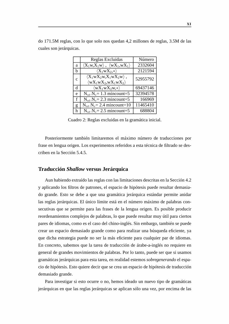
Basándonos en estos resultados construimos una gramática inicial mediante la
exclusión de ciertos patrones (idénticos y monótonos), y aplicando filtrosmincount
como se recoge en el Cuadro 2. En total, con este procedimiento estamos excluyen-
XI
do 171.5M reglas, con lo que solo nos quedan 4,2 millones de reglas, 3.5M de las
cuales son jerárquicas.
Reglas Excluidas Númeroa 〈X1w,X1w〉 , 〈wX1,wX1〉 2332604b 〈X1wX2,∗〉 2121594
〈X1wX2w,X1wX2w〉 ,c〈wX1wX2,wX1wX2〉
52955792
d 〈wX1wX2w,∗〉 69437146e Nnt.Ne= 1.3 mincount=5 32394578f Nnt.Ne= 2.3 mincount=5 166969g Nnt.Ne= 2.4 mincount=10 11465410h Nnt.Ne= 2.5 mincount=5 688804
Cuadro 2: Reglas excluidas en la gramática inicial.
Posteriormente también limitaremos el máximo número de traducciones por
frase en lengua origen. Los experimentos referidos a esta técnica de filtrado se des-
criben en la Sección 5.4.5.
Traducción Shallow versus Jerárquica
Aun habiendo extraído las reglas con las limitaciones descritas en la Sección 4.2
y aplicando los filtros de patrones, el espacio de hipótesis puede resultar demasia-
do grande. Esto se debe a que una gramática jerárquica estándar permite anidar
las reglas jerárquicas. El único límite está en el número máximo de palabras con-
secutivas que se permite para las frases de la lengua origen.Es posible producir
reordenamientos complejos de palabras, lo que puede resultar muy útil para ciertos
pares de idiomas, como es el caso del chino-inglés. Sin embargo, también se puede
crear un espacio demasiado grande como para realizar una búsqueda eficiente, ya
que dicha estrategia puede no ser la más eficiente para cualquier par de idiomas.
En concreto, sabemos que la tarea de traducción de árabe-a-inglés no requiere en
general de grandes movimientos de palabras. Por lo tanto, puede ser que si usamos
gramáticas jerárquicas para esta tarea, en realidad estemossobregenerandoel espa-
cio de hipótesis. Esto quiere decir que se crea un espacio de hipótesis de traducción
demasiado grande.
Para investigar si esto ocurre o no, hemos ideado un nuevo tipo de gramáticas
jerárquicas en que las reglas jerárquicas se aplican sólo una vez, por encima de las

XII
cuales hay que aplicar la regla ‘glue’. Denominamosgramáticas shallowa estas
gramáticas, por comparación con las gramáticas jerárquicas habituales1, en las que
el límite de anidamiento se establece indirectamente a través de un número máximo
de palabras consecutivas (típicamente 10-12 palabras).
Las reglas utilizadas para una gramáticashallow pueden expresarse como se
muestra en el Cuadro 3.
Gramática ShallowS→〈X,X〉 regla ‘glue’ 1S→〈S X,S X〉 regla ‘glue’ 2V→〈s,t〉 reglas léxicasX→〈γ,α,∼〉 , γ, α ∈ V ∪T+ reglas jerárquicas
Cuadro 3: Reglas de una gramática jerárquicashallow.
La Figura 3 muestra una gramática jerárquica definida por seis reglas. Para la
oración que queremos traducirs1s2s3s4 existen dos árboles de análisis posibles, que
se corresponden a las derivacionesR1R4R3R5 y R2R1R3R5R6. Cada árbol muestra
también la traducción correspondiente.
Al comparar los dos árboles vemos que el de la izquierda saca una traducción
más reordenada, a través de las reglas jerárquicasR3 y R4, anidadas sobreR5.
Esto puede ser interesante para la traducción entre ciertospares de lenguas que
requieren reordenamientos más agresivos, pero en pares de lenguas más cercanos
crearía hipótesis innecesarias.
R1: S→〈X ,X〉R2: S→〈S X ,S X〉R3: X→〈X s3,t5 X〉R4: X→〈X s4,t3 X〉R5: X→〈s1 s2,t1 t2〉R6: X→〈s4,t7〉
Figura 3: Ejemplo de traducción jerárquica con dos árboles de análisis sintáctico queusan diferentes anidamientos de reglas para la misma oración de entradas1s2s3s4.
Para evitarlo, podemos reescribir la gramática de la siguiente manera:
1Que consecuentemente a veces denominamos en inglésfull hierarchical grammars.

XIII
1. Se sustituye el no terminalX de la parte derecha de las reglas por un no
terminalV enR3, R4:
R3:X→〈V s3,t5 V 〉
R4:X→〈V s4,t3 V 〉
2. Las reglas léxicas (frases) se aplican en celdasV . Por lo tanto:
R5:V→〈s1 s2,t1 t2〉
R6:V→〈s4,t7〉
Con estas sencillas modificaciones estamos evitando que se aniden reglas
jerárquicas sobre otras reglas que no sean frases léxicas, es decir, reglas que so-
lo traducen secuencias de palabras. Por lo tanto, ahora la hipótesis de traducción
t3t5t1t2 no puede ser generada. En este sentido, lo que estamos haciendo es filtrar
todas aquellas derivaciones que anidan reglas jerárquicasmás de una vez.
En la Sección 5.4.4 contrastamos calidad y velocidad de una gramáticashallow
y otra tradicional para la tarea de traducción de árabe a inglés utilizando el decodi-
ficador HCP, descrito en la Sección 4.3. Mientras que la calidad se mantiene, la
velocidad de traducción aumenta considerablemente.
Extensiones a las Gramáticas Shallow
Las gramáticas son muy flexibles. Se pueden definir muchas variaciones, dando
lugar cada una de ellas a un espacio de hipótesis diferente.
Por ejemplo, hemos visto que limitar el numero máximo de anidamientos de las
reglas a uno es una buena estrategia para la tarea de traducción de árabe a inglés.
También puede considerarse la posibilidad de limitar ciertas reglas en la etapa de
análisis a un ámbito definido por un mínimo y un máximo de palabras consecutivas.
O, si se detecta un problema concreto con un modelo para una tarea específica de
traducción, se podrían añadir reglasad hocpara permitir que el decodificador en-
cuentre la hipótesis correcta. Al final, el objetivo es construir de manera eficiente el
espacio de búsqueda necesario para cada tarea de traducción.
En resumen, en esta tesis se proponen las siguientes estrategias de diseño para
obtener espacios de búsqueda más eficientes:
1. Gramáticasshallow-N . Esta técnica es una extensión natural de las gramáti-
casshallow, y básicamente limita los anidamientos a un número arbitrario N .

XIV
El Cuadro 4 muestra gramáticasshallow-N conN = 1, 2. Cuanto mayor sea
N , más cerca estará de una gramática jerárquica estándar. La descripción de-
tallada puede hallarse en la Sección 5.6. Experimentos paraestas gramáticas
pueden encontrarse en la Sección 6.6.2.
2. Concatenación de frases jerárquicas a niveles bajos. Aumentamos el espacio
de búsqueda al permitir que ciertas frases jerárquicas se concatenen directa-
mente. El procedimiento se explica en detalle en la Sección 5.6.2. Experimen-
tos con esta extensión se realizan en la Sección 6.5.2.
3. Filtrado por número de palabras consecutivas. Es una técnica sencilla de fil-
trado que se puede aplicar durante la etapa de análisis sintáctico. Se impone
que ciertas reglas se apliquen solo si cubren un intervalo entre un número
mínimo y uno máximo de palabras consecutivas. Esta técnica se explica en la
Sección 5.6.3; los experimentos pueden encontrarse en la Sección 6.6.2.
gramática reglas incluidasS-1 S→〈X1,X1〉 S→〈SX1,SX1〉 reglas ‘glue’
X0→〈γ,α〉 , γ, α ∈ T+ frases léxicasX1→〈γ,α,∼〉 , γ, α ∈ X0 ∪T+ reglas jerárquicas de nivel 1
S-2 S→〈X2,X2〉 S→〈SX2,SX2〉 reglas ‘glue’X0→〈γ,α〉 , γ, α ∈ T+ frases léxicasX1→〈γ,α,∼〉 , γ, α ∈ X0 ∪T+ reglas jerárquicas de nivel 1X2→〈γ,α,∼〉 , γ, α ∈ X1 ∪T+ reglas jerárquicas de nivel 2
Cuadro 4: Reglas para una gramáticashallow-N , conN = 1, 2.
Traducción Jerárquica con Celosías
En esta sección hablaremos del nuevo decodificador que denominamosHiFST.
En términos generales, este decodificador funciona de una manera muy similar a un
decodificador de poda hipercúbica. Sin embargo, en lugar de construir las listas en
cada celda de la rejilla CYK, construimos celosías que contienen todas las posibles
traducciones de la frase origen cubierto por dicha celda. Demanera similar a HCP,
en la celda superior obtendremos la celosía con hipótesis detraducción para toda
la oración de entrada. La Figura 4 muestra un ejemplo de traducción para el que
XV
se usan celosías en vez de listas. A priori, vemos que esto podría ser beneficioso
porque:
1. Las celosías son representaciones mucho más compactas deun espacio que
contiene lask mejores hipótesis. Esto se traduce en espacios de búsqueda más
grandes, menos errores de búsqueda y listas más ricas de hipótesis que pueden
conducir a una mejor optimización enMinimum Error Training[Och, 2003]
y mejorrescoring.
2. Las celosías implementadas como transductores (WFSTs) tienen la ventaja de
aceptar cualquier operación definida sobre elsemianillode los WFSTs. Esto
es, podemos realizar determinización, minimización, composición, etcétera.
Ya en la Sección 4.5 contrastamos HCP con un traductor (implementado con
celosías) basado en frases que prácticamente carece de errores de búsqueda. Pese
a que el experimento se realiza sobre un espacio de búsqueda sencillo, detectamos
un número notable de errores de búsqueda con HCP. Esto nos sugiere que para
gramáticas más complejas tendremos más errores de búsqueda.
Puesto que las celosías representan hipótesis de una maneramucho más com-
pacta que las listas, las necesidades de poda serán menores;por lo tanto se puede
afirmar que mediante el uso de celosías estamos trabajando enla práctica con un
espacio de búsqueda que es un superconjunto del creado por eldecodificador de la
poda hipercúbica. Pero las ideas subyacentes de ambos decodificadores son exac-
tamente las mismas, ya que los dos han de analizar la frase de origen y almacenan
subconjuntos del espacio de búsqueda que, guiados por losbackpointersa través de
la rejilla de celdas CYK, se van combinando hasta crear el conjunto de traducciones
correspondientes a la oración de entrada.
Concluimos esta sección presentando una visión general de este nuevo decodi-
ficador, llamadoHiFST, representado en la Figura 5.
HiFST funciona en tres etapas:
1. El algoritmo de análisis CYK se aplica a la frase de origen.Se construye
una rejilla que almacena el uso de reglas y losbackpointersnecesarios para
obtener las posibles derivaciones.
2. Utilizando losbackpointers, se inspeccionan de forma recursiva las celdas re-
levantes de la rejilla. En cada celda construimos una celosía con las hipótesis

XVI
Figura 4: HiFST construye el mismo espacio de búsqueda utilizando celosías.
Figura 5: El sistema de traducciónHiFST.

XVII
de traducción. Una vez acabado el algoritmo tendremos en la celda supe-
rior la celosía que contiene todas las traducciones disponibles para la oración
de origen. Como veremos, por una cuestión de eficiencia no se construye la
celosía de palabras de una sola pasada, sino que se utilizan punteros a celosías
inferiores. En un segundo paso se realiza la expansión para obtener el espacio
completo de hipótesis. En cualquier caso, la poda durante laconstrucción de
la celosía de traducción puede ser necesaria en esta etapa.
3. Una vez que tenemos la celosía de traducciones para toda lafrase de entrada,
se aplica el modelo de lenguaje. Las hipótesis 1-best (correspondiente a la
ruta con menor coste) serán usadas para la evaluación. No obstante, se suele
aplicar una poda menos estricta a la celosía de traducción, lo que permite al-
macenar cientos de miles de hipótesis que serán útiles para etapas posteriores
derescoringo combinación de sistemas.
Algoritmo de Construcción de Celosías
Cada celda(N, x, y) de la rejilla CYK contiene un conjunto de índices de reglas
R(N, x, y). Para un índicer/Rr ∈ R(N, x, y), la reglaN → 〈γr,αr〉 se ha usado
al menos en una derivación que pasa por esta celda.
Para cada reglaRr, r ∈ R(N, x, y) construimos una celosíaL(N, x, y, r), para
lo que utilizamos la traducción de la regla, que consiste en una serie deelementos(o
combinación arbitraria de terminales y no terminales) consecutivos,αr = αr1...α
r|αr |.
Estas celosías se construyen por concatenación de pequeñascelosías asociadas a
cada elementoαri . Si este elemento es una palabra o terminal, la celosía es trivial
(dos estados unidos por un arco que codifica la palabra traducida). Si por el contrario
es un no terminal, entonces existe unbackpointer(creado durante el análisis CYK)
que permite crear (recursivamente) una celosíaL(N ′, x′, y′) a nivel inferior, de la
que depende de esta regla.
La Figura 6 muestra el algoritmo recursivo que empleaHiFST para construir
la celosía en cada celda. El algoritmo utiliza memoización (memoization): si una
celosía asociada a una celda ya existe, entonces se ha guardado y solo toca devolver-
la (línea 2). De lo contrario, hay que construirla primero. Para todas las reglas, se
revisa cada elemento de la traducción (líneas 3 y 4). Si es terminal (línea 5), se cons-
truye el aceptor trivial descrito anteriormente. De lo contrario (línea 6) se devuelve
la celosía asociada a subackpointer(líneas 7 y 8). La celosía para la regla com-

XVIII
pleta se construye por concatenación de las celosías para cada elemento (línea 9).
La celosía para cada celda se construye por unión de las celosías asociadas a todas
las reglas que aplican en dicha celda (línea 10). Finalmente, se reduce su tamaño
mediante operaciones estándar de transductores (líneas 11, 12 y 13), descritas en la
Sección 2.2.2.
1 función buildFst(N,x,y)2 if ∃ L(N, x, y) returnL(N, x, y)3 for r ∈ R(N, x, y), Rr : N → 〈γ,α〉4 for i = 1...|α|5 if αi ∈ T , L(N, x, y, r, i) = A(αi)6 else7 (N ′, x′, y′) = BP (αi)8 L(N, x, y, r, i) = buildFst(N ′, x′, y′)9 L(N, x, y, r)=
⊗
i=1..|α|L(N, x, y, r, i)
10 L(N, x, y) =⊕
r∈R(N,x,y) L(N, x, y, r)
11 fstRmEpsilonL(N, x, y)12 fstDeterminizeL(N, x, y)13 fstMinimizeL(N, x, y)14 returnL(N, x, y)
Figura 6: Pseudocódigo del algoritmo recursivo que construye el espacio de búsque-da.
A continuación introduciremos un detalle de implementación muy relevante que
denominamos traducción demorada. La Sección 6.3 explica este y otros detalles al-
gorítmicos, incluyendo la poda durante la construcción de la celosía de traducción
(Sección 6.3.4.2) o la estrategia de borrado de palabras (Sección 6.3.5). La Sec-
ción 6.4 explica qué pasos son necesarios para realizar optimización con MET.
Traducción Demorada
La inclusión directa de celosías de nivel inferior conduce en muchos casos a
una explosión de memoria. Para evitarlo, construimos las celosías usando unos ar-
cos especiales que sirven como punteros a dichas celosías denivel inferior. Una
vez acabado el algoritmo de construcción de la celosía de traducción, la celosía
L(S, 1, J) asociada a la celda superior contiene punteros a celosías defilas infe-
riores. Entonces utilizamos una única operaciónfstreplace[Allauzenet al., 2007]
que expande recursivamente la celosía sustituyendo los punteros por sus correspon-
dientes celosías, hasta que no queda ningún puntero y, por lotanto, el espacio de

XIX
hipótesis solo contiene palabras. A esta técnica la denominamos traducción de-
morada (delayed translation).
Figura 7: Técnica de traducción demorada (Delayed Translation) durante la cons-trucción de las celosías.
Para entender mejor esta técnica y su necesidad, consideremos una situación
hipotética como la representada en la Figura 7: estamos ejecutando el algoritmo de
construcción de celosías y ya hemos construido una celosía de una de las celdas
de la fila1 en la red de CYK (L1). En algún punto de la ejecución tenemos que
construir una celosía nuevaL3 correspondiente la fila3, y que requiere a través
de diversas reglas la celosíaL1, de jerarquía inferior. Dado que hay más de un
puntero en la celosíaL3, L1 podría repetirse más de una vez enL3. Es fácil prever
el riesgo de explosión por crecimiento exponencial del número de estados. Para
resolver este problema, se usa un arco especial enL3 que apunta aL1, con lo que se
demorala construcción de hipótesis de traducción hasta el final, cuando se realiza la
expansión de las celosías. En conjunto, este procedimientocontrola el tamaño de las
celosías asociadas a las celdas de la rejilla CYK que visitamos durante el algoritmo
de construcción de la celosía final de traducción.
Es importante destacar que ciertas operaciones estándar enestas WFSTs
—como la reducción de tamaño sin pérdida a través de determinización y
minimización— todavía se pueden realizar. Debido a la existencia de múltiples re-

XX
0
1t1
2g(X,1,2)
3g(X,1,1)
5
g(X,3,1)
7
t2
g(X,3,1)
4t10
6t10
g(X,3,1)
g(X,1,1)
0
3g(X,1,1)
2g(X,1,2)
1
t1
4
g(X,3,1)
t10
6
g(X,3,1)
t2
5t10
g(X,1,1)
Figura 8: Ejemplo de aplicación de operaciones WFST para celosías con traduc-ción demorada. En este caso se muestra un transductor antes [arriba] y después deminimizar [abajo].
glas jerárquicas que comparten las mismas dependencias a través de susbackpoin-
ters, estas operaciones pueden reducir considerablemente el tamaño de una celosía
con arcos puntero; la Figura 8 muestra un pequeño ejemplo. Sibien la reducción de
número de estados puede ser importante, no es posible eliminar completamente la
redundancia, ya que pueden aparecer hipótesis duplicadas una vez expandidos los
arcos puntero, identificados como una funcióng.
Experimentos conHiFST
Para esta tesis usamos el traductorHiFST con tres tareas de traducción dife-
rentes:
Árabe a inglés. La descripción detallada de los experimentos, resultados y
correspondientes discusiones se encuentran en la Sección 6.5. En particular,
contrastamos la calidad de nuestro sistema de traducción depoda hipercúbi-
ca conHiFST. Cabe destacar queHiFST es capaz de construir el espacio de
hipótesis de la gramáticashallow-1 sin necesidad de poda, debido a la com-
pacidad de las celosías. En este contexto se realiza una búsqueda exacta de
la mejor hipótesis de traducción, lo que justifica las mejoras de calidad intro-

XXI
ducidas porHiFST. Asimismo,HiFST es parte del sistema ganador del NIST
2009, enviado por el departamento de ingeniería de la Universidad de Cam-
bridge (CUED) para esta tarea de traducción. También estudiamos siHiFST
puede mejorar utilizando probabilidades marginales (semianillo logarítmico).
Chino a inglés. En la Sección 6.6 se describen en detalle estos experimentos,
que incluyen un contraste con HCP; las conclusiones son similares pese a que
ahora es necesario realizar traducción jerárquica estándar y se realiza poda
durante la construcción de la celosía de traducción. En estasección también se
experimenta con las gramáticasshallow-N y se estudian diversos parámetros
de poda durante la construcción de la celosía de traducción para ver cómo
afecta en velocidad y calidad.
Castellano a inglés. En la Sección 6.7 se muestran algunos experimentos en
que vemos queHiFST es capaz de obtener calidades comparables al estado
del arte utilizandoHiFST con gramáticasshallow.
Conclusiones
En esta tesis nos centramos en dos aspectos fundamentales dela traducción
automática estadística: el diseño deespacio de hipótesisy el algoritmo de búsqueda,
en el marco de decodificación de frases jerárquicas.
El Capítulo 5 se ocupa del diseño eficiente de espacios de hipótesis. Para ello
proponemos diversas técnicas, entre las que cabe destacar muy especialmente las
gramáticasshallow, que limitan directamente la anidación de reglas, con la idea
de evitar problemas de sobregeneración y ambigüedad que surgen de espacios de
búsqueda demasiado grandes, lo que conduce a errores de búsqueda durante la cons-
trucción del espacio de hipótesis.
El Capítulo 4 y el Capítulo 6 se ocupan del problema algorítmico. En primer
lugar, desarrollamos un decodificador de poda hipercúbica.Proponemos dos pe-
queñas mejoras, llamadassmart memoizationy spreading neighbourhood explo-
ration, que tratan de llegar a una mayor eficiencia en términos de usode memoria y
de rendimiento, respectivamente.
Además, este traductor nos sirve de referencia para el nuevosistema de tra-
ducciónHiFST, explicado en detalle a lo largo del Capítulo 6. Utiliza celosías que

XXII
contienen hipótesis de traducción, implementadas mediante máquinas de estados
finitos. Para ello empleamos la libreríaOpenFSTde Google[Allauzenet al., 2007].
Este nuevo algoritmo puede verse como una evolución de HCP, en que se utilizan
celosías en vez de listas de hipótesis, lo que lleva a mayor eficiencia y compacidad
en la representación de las mismas en memoria. Al implementar estas celosías me-
diante transductores (WFSTs) tenemos la ventaja añadida decontar con operaciones
estándar como minimización, determinización, composición, etcétera, que simplifi-
can considerablemente la implementación de dicho algoritmo.
UtilizandoHiFST con nuestras gramáticasshallowconseguimos crear espacios
de hipótesis exactos, lo que implica que evitamos errores debúsqueda que provienen
de podar durante el proceso mismo de la construcción del espacio de hipótesis.
Hemos visto que es posible obtener con una gramáticashallow-1 una calidad si-
milar a una gramática tradicional jerárquica para ciertos pares de traducción en que
no es necesario reordenar excesivamente las palabras. Además, al tratarse de un
espacio de búsqueda lo suficientemente pequeño como para queHiFST evite podas
durante la construcción del espacio de hipótesis, la velocidad de traducción aumenta
considerablemente.

Contents
1. Introduction 1
1.1. Motivation . . . . . . . . . . . . . . . . . . . . . . . . . . . . . . . 1
1.2. Objectives . . . . . . . . . . . . . . . . . . . . . . . . . . . . . . . 4
1.3. Thesis Organization . . . . . . . . . . . . . . . . . . . . . . . . . . 5
2. Foundations 9
2.1. Introduction . . . . . . . . . . . . . . . . . . . . . . . . . . . . . . 9
2.2. Finite-State Technology . . . . . . . . . . . . . . . . . . . . . . . . 10
2.2.1. Semirings . . . . . . . . . . . . . . . . . . . . . . . . . . . 13
2.2.1.1. Weighted Finite-state Transducers . . . . . . . . 14
2.2.2. Standard Weighted Finite-state Operations . . . . . . .. . 16
2.2.2.1. Inversion . . . . . . . . . . . . . . . . . . . . . . 16
2.2.2.2. Concatenation . . . . . . . . . . . . . . . . . . . 16
2.2.2.3. Union . . . . . . . . . . . . . . . . . . . . . . . 17
2.2.2.4. Epsilon Removal . . . . . . . . . . . . . . . . . . 18
2.2.2.5. Determinization and Minimization . . . . . . . . 18
2.2.2.6. Composition . . . . . . . . . . . . . . . . . . . . 20
2.3. Parsing . . . . . . . . . . . . . . . . . . . . . . . . . . . . . . . . 21
2.3.1. CYK Parsing . . . . . . . . . . . . . . . . . . . . . . . . . 23
2.3.1.1. Implementation . . . . . . . . . . . . . . . . . . 25
2.3.2. Some Historical Notes on Parsing . . . . . . . . . . . . . . 27
2.3.3. Relationship between Parsing and Automata . . . . . . . .29
2.4. Conclusions . . . . . . . . . . . . . . . . . . . . . . . . . . . . . . 31

XXIV Contents
3. Machine Translation 33
3.1. Introduction . . . . . . . . . . . . . . . . . . . . . . . . . . . . . . 33
3.2. Brief Historical Review . . . . . . . . . . . . . . . . . . . . . . . . 34
3.2.1. Interlingua Systems . . . . . . . . . . . . . . . . . . . . . . 35
3.2.2. Transfer-based systems . . . . . . . . . . . . . . . . . . . . 35
3.2.3. Direct Systems . . . . . . . . . . . . . . . . . . . . . . . . 36
3.3. Performance . . . . . . . . . . . . . . . . . . . . . . . . . . . . . . 37
3.3.1. Automatic Evaluation Metrics . . . . . . . . . . . . . . . . 38
3.3.2. Human Evaluation Metrics . . . . . . . . . . . . . . . . . . 40
3.4. Statistical Machine Translation Systems . . . . . . . . . . .. . . . 41
3.4.1. Language Model . . . . . . . . . . . . . . . . . . . . . . . 42
3.4.2. Maximum Entropy Frameworks and MET . . . . . . . . . . 43
3.4.3. Model Estimation and Optimization . . . . . . . . . . . . . 43
3.4.4. Word Alignment and Translation Unit . . . . . . . . . . . . 45
3.5. Phrase-Based systems . . . . . . . . . . . . . . . . . . . . . . . . . 48
3.5.1. TTM . . . . . . . . . . . . . . . . . . . . . . . . . . . . . 50
3.5.2. The n-gram-based System . . . . . . . . . . . . . . . . . . 51
3.6. Syntactic Phrase-based systems . . . . . . . . . . . . . . . . . . .. 52
3.7. Reranking and System Combination . . . . . . . . . . . . . . . . . 53
3.8. WFSTs for Translation . . . . . . . . . . . . . . . . . . . . . . . . 54
3.9. Conclusions . . . . . . . . . . . . . . . . . . . . . . . . . . . . . . 54
4. Hierarchical Phrase-based Translation 57
4.1. Introduction . . . . . . . . . . . . . . . . . . . . . . . . . . . . . . 57
4.2. Hierarchical Phrase-Based Translation . . . . . . . . . . . .. . . . 58
4.3. Hypercube Pruning Decoder . . . . . . . . . . . . . . . . . . . . . 60
4.3.1. General overview . . . . . . . . . . . . . . . . . . . . . . . 60
4.3.2. K-best decoding with Hypercube Pruning . . . . . . . . . . 62
4.3.2.1. Applying the Language Model . . . . . . . . . . 65
4.4. Two Refinements in the Hypercube Pruning Decoder . . . . . .. . 66
4.4.1. Smart Memoization . . . . . . . . . . . . . . . . . . . . . . 68
4.4.2. Spreading Neighbourhood Exploration . . . . . . . . . . . 68
4.5. A Study of Hiero Search Errors in Phrase-Based Translation . . . . 69
4.6. Related Work . . . . . . . . . . . . . . . . . . . . . . . . . . . . . 71
4.6.1. Hiero Key Papers . . . . . . . . . . . . . . . . . . . . . . . 72

Contents XXV
4.6.2. Extensions and Refinements to Hiero . . . . . . . . . . . . 72
4.6.3. Hierarchical Rule Extraction . . . . . . . . . . . . . . . . . 73
4.6.4. Contrastive Experiments and Other Hiero Contributions . . 74
4.7. Conclusions . . . . . . . . . . . . . . . . . . . . . . . . . . . . . . 74
5. Hierarchical Grammars 77
5.1. Introduction . . . . . . . . . . . . . . . . . . . . . . . . . . . . . . 77
5.2. Experimental Framework . . . . . . . . . . . . . . . . . . . . . . . 78
5.3. Preliminary Discussions . . . . . . . . . . . . . . . . . . . . . . . 79
5.3.1. Completeness of the Model . . . . . . . . . . . . . . . . . 79
5.3.2. Do We Actually Need the Complete Grammar? . . . . . . . 82
5.4. Filtering Strategies for Practical Grammars . . . . . . . .. . . . . 83
5.4.1. Rule Patterns . . . . . . . . . . . . . . . . . . . . . . . . . 83
5.4.2. Quantifying Pattern Contribution . . . . . . . . . . . . . . .87
5.4.3. Building a Usable Grammar . . . . . . . . . . . . . . . . . 92
5.4.4. Shallow versus Fully Hierarchical Translation . . . .. . . . 93
5.4.5. Individual Rule Filters . . . . . . . . . . . . . . . . . . . . 96
5.4.6. Revisiting Pattern-based Rule Filters . . . . . . . . . . .. . 98
5.5. Large Language Models and Evaluation . . . . . . . . . . . . . . .99
5.6. Shallow-N grammars and Extensions . . . . . . . . . . . . . . . . 100
5.6.1. Shallow-N Grammars . . . . . . . . . . . . . . . . . . . . 101
5.6.2. Low Level Concatenation for Struct. Long Dist. Movement 102
5.6.3. Minimum and Maximum Rule Span . . . . . . . . . . . . . 104
5.7. Conclusions . . . . . . . . . . . . . . . . . . . . . . . . . . . . . . 105
6. HiFST: Hierarchical Translation with WFSTs 107
6.1. Introduction . . . . . . . . . . . . . . . . . . . . . . . . . . . . . . 107
6.2. From HCP toHiFST . . . . . . . . . . . . . . . . . . . . . . . . . 108
6.3. Hierarchical Translation with WFSTs . . . . . . . . . . . . . . .. 111
6.3.1. Lattice Construction Over the CYK Grid . . . . . . . . . . 112
6.3.1.1. An Example of Phrase-based Translation . . . . . 113
6.3.1.2. An Example of Hierarchical Translation . . . . . 115
6.3.2. A Procedure for Lattice Construction . . . . . . . . . . . . 117
6.3.3. Delayed Translation . . . . . . . . . . . . . . . . . . . . . 118
6.3.4. Pruning in Lattice Construction . . . . . . . . . . . . . . . 121

XXVI Contents
6.3.4.1. Full Pruning . . . . . . . . . . . . . . . . . . . . 121
6.3.4.2. Pruning in Search . . . . . . . . . . . . . . . . . 122
6.3.5. Deletion Rules . . . . . . . . . . . . . . . . . . . . . . . . 123
6.3.6. Revisiting the Algorithm . . . . . . . . . . . . . . . . . . . 124
6.4. Alignment for MET optimization . . . . . . . . . . . . . . . . . . . 124
6.4.1. Alignment via Hypercube Pruning decoder . . . . . . . . . 127
6.4.2. Alignment via FSTs . . . . . . . . . . . . . . . . . . . . . 128
6.4.2.1. Using a Reference Acceptor . . . . . . . . . . . . 131
6.4.2.2. Extracting Feature Values from Alignments . . . 132
6.5. Experiments on Arabic-to-English . . . . . . . . . . . . . . . . .. 133
6.5.1. Contrastive Experiments with HCP . . . . . . . . . . . . . 134
6.5.1.1. Search Errors . . . . . . . . . . . . . . . . . . . 135
6.5.1.2. Lattice/k-best Quality . . . . . . . . . . . . . . . 136
6.5.1.3. Translation Speed . . . . . . . . . . . . . . . . . 136
6.5.2. Shallow-N Grammars and Low-level Concatenation . . . . 136
6.5.3. Experiments using the Log-probability Semiring . . .. . . 138
6.5.4. Experiments with Features . . . . . . . . . . . . . . . . . . 140
6.5.5. Combining Alternative Segmentations . . . . . . . . . . . .141
6.6. Experiments on Chinese-to-English . . . . . . . . . . . . . . . .. 142
6.6.1. Contrastive Translation Experiments with HCP . . . . .. . 143
6.6.1.1. Search Errors . . . . . . . . . . . . . . . . . . . 144
6.6.1.2. Lattice/k-best Quality . . . . . . . . . . . . . . . 144
6.6.2. Experiments with Shallow-N Grammars . . . . . . . . . . 144
6.6.3. Pruning in Search . . . . . . . . . . . . . . . . . . . . . . . 146
6.7. Experiments on Spanish-to-English Translation . . . . .. . . . . . 148
6.7.1. Filtering by Patterns and Mincounts . . . . . . . . . . . . . 150
6.7.2. Hiero Shallow Model . . . . . . . . . . . . . . . . . . . . . 150
6.7.3. Filtering by Number of Translations . . . . . . . . . . . . . 151
6.7.4. Revisiting Patterns and Class Mincounts . . . . . . . . . .. 151
6.7.5. Rescoring and Final Results . . . . . . . . . . . . . . . . . 152
6.8. Conclusions . . . . . . . . . . . . . . . . . . . . . . . . . . . . . . 152
7. Conclusions 155
Bibliography 159

List of Figures
1. Decodificador de poda hipercúbica (HCP). . . . . . . . . . . . . . .VII
2. HCP construye el espacio de búsqueda mediante listas de hipótesis. VIII
3. Ejemplo de traducción jerárquica. . . . . . . . . . . . . . . . . . .XII
4. HiFST construye el mismo espacio de búsqueda utilizando celosías. XVI
5. El sistema de traducciónHiFST. . . . . . . . . . . . . . . . . . . .XVI
6. Pseudocódigo del algoritmo recursivo. . . . . . . . . . . . . . . .. XVIII
7. Técnica de traducción demorada. . . . . . . . . . . . . . . . . . . .XIX
8. Aplicación de operaciones WFST con traducción demorada.. . . . XX
1.1. Research areas versus HiFST. . . . . . . . . . . . . . . . . . . . . . 5
2.1. Trivial finite automata. . . . . . . . . . . . . . . . . . . . . . . . . 12
2.2. Trivial finite transducer. . . . . . . . . . . . . . . . . . . . . . . . 13
2.3. Trivial weighted finite-state transducer. . . . . . . . . . .. . . . . 15
2.4. An inverted finite-state transducer. . . . . . . . . . . . . . . .. . . 17
2.5. A concatenation example. . . . . . . . . . . . . . . . . . . . . . . 17
2.6. Union example. . . . . . . . . . . . . . . . . . . . . . . . . . . . . 18
2.7. An epsilon removal example. . . . . . . . . . . . . . . . . . . . . 19
2.8. Determinization example. . . . . . . . . . . . . . . . . . . . . . . . 20
2.9. Minimization example. . . . . . . . . . . . . . . . . . . . . . . . . 21
2.10. Composition example. . . . . . . . . . . . . . . . . . . . . . . . . 22
2.11. Grid with rules and backpointers after the parser has finished. . . . . 26
2.12. A simple example of a Recursive Transition Network. . .. . . . . . 30
3.1. Triangle of Vauquois. . . . . . . . . . . . . . . . . . . . . . . . . . 34
3.2. Model Estimation. . . . . . . . . . . . . . . . . . . . . . . . . . . 44

XXVIII List of Figures
3.3. Parameter optimization and test translation. . . . . . . .. . . . . . 45
3.4. An example of word alignments. . . . . . . . . . . . . . . . . . . . 45
3.5. An example of phrases extracted from alignments in Figure 3.4. . . 48
3.6. An example of tuples extracted from alignments inf Figure 3.4. . . 51
3.7. An example of hierarchical phrases, from alignments inFigure 3.4. . 52
4.1. General flow of a hypercube pruning decoder (HCP). . . . . .. . . 61
4.2. Grid with rules and backpointers after the parser has finished. . . . . 63
4.3. Example of a hypercube of order 2. . . . . . . . . . . . . . . . . . . 65
4.4. Now a cost for each hypothesis has to be added on the fly. . .. . . . 66
4.5. Situation with 9 hyps extracted and the 10th hyp goes next. . . . . . 67
4.6. Spreading neighbourhood exploration within a hypercube. . . . . . 69
5.1. Model versus reality. . . . . . . . . . . . . . . . . . . . . . . . . . 79
5.2. Example of multiple translation sequences from a simple grammar. . 80
5.3. Example of multiple translation sequences from a simple grammar. . 95
5.4. Movement allowed by two grammars. . . . . . . . . . . . . . . . . 104
6.1. HCP builds the search space using lists. . . . . . . . . . . . . .. . 109
6.2. HiFST builds the same search space using lattices. . . . . . . . . . 110
6.3. TheHiFST decoder. . . . . . . . . . . . . . . . . . . . . . . . . . . 111
6.4. Translation rules, CYK grid and production of the translation lattice. 113
6.5. A lattice encoding two target sentences. . . . . . . . . . . . .. . . 115
6.6. Translation fors1s2s3, with rulesR3, R4, R6,R7,R8. . . . . . . . . 116
6.7. A lattice encoding four target sentences. . . . . . . . . . . .. . . . 117
6.8. Recursive Lattice Construction. . . . . . . . . . . . . . . . . . .. . 118
6.9. Delayed translation during lattice construction. . . .. . . . . . . . 119
6.10. Delayed translation WFST before and after minimization. . . . . . . 121
6.11. Pseudocode for Pruning in Search. . . . . . . . . . . . . . . . . .. 123
6.12. Transducers for filtering up to one or two consecutive deletions. . . 124
6.13. Recursive lattice construction, extended. . . . . . . . .. . . . . . . 125
6.14. Global pseudocode forHiFST. . . . . . . . . . . . . . . . . . . . . 125
6.15. Alignment is needed to extract features for optimization. . . . . . . 126
6.16. An example of a suffix array used on one reference translation. . . . 128
6.17. FST encoding simultaneously a rule derivation and thetranslation. . 129
6.18. FST encoding two different rule derivations for the same translation. 130

List of Figures XXIX
6.19. Construction of a substring acceptor. . . . . . . . . . . . . .. . . . 130
6.20. One arc from a rule acceptor that assignsK feature weights. . . . . 132
6.21. A rule acceptor that assignsK feature weights to each rule. . . . . . 133


List of Tables
1. Reglas de una gramática estándar jerárquica. . . . . . . . . . .. . . VI
2. Reglas excluidas en la gramática inicial. . . . . . . . . . . . . .. . XI
3. Reglas de una gramática jerárquicashallow. . . . . . . . . . . . . . XII
4. Reglas para una gramáticashallow-N , conN = 1, 2. . . . . . . . . XIV
2.1. A state matrix for a simple automaton . . . . . . . . . . . . . . . .11
2.2. Semiring examples. . . . . . . . . . . . . . . . . . . . . . . . . . . 14
2.3. Chomsky’s hierarchy (extended) . . . . . . . . . . . . . . . . . . .29
4.1. Contrast of grammars.T is the set of terminals. . . . . . . . . . . . 69
4.2. Phrase-based TTM and Hiero performance onmt02-05-tune . . . . 71
5.1. Hierarchical rule patterns (〈source,target〉) for mt02-05-tune(I). . . 84
5.2. Hierarchical rule patterns (〈source,target〉) for mt02-05-tune(II). . . 85
5.3. Hierarchical rule patterns (〈source,target〉) for mt02-05-tune(and III). 86
5.4. Scores for grammars using one single hierarchical pattern (I). . . . . 89
5.5. Scores for grammars using one single hierarchical pattern (II). . . . 90
5.6. Scores for grammars using one single hierarchical pattern (and III). . 91
5.7. Scores for grammars adding a single rule pattern to the new baseline. 91
5.8. Grammar configurations, with rules in millions. . . . . . .. . . . . 92
5.9. Rules excluded from the initial grammar. . . . . . . . . . . . .. . . 94
5.10. Rules contained in the standard hierarchical grammar. . . . . . . . . 94
5.11. Rules contained in the shallow hierarchical grammar.. . . . . . . . 95
5.12. Translation performance and time for full vs. shallowgrammars. . . 96
5.13. Impact of general rule filters on translation, time andnumber of rules. 97
5.14. Top five hierarchical 1-best rule usage. . . . . . . . . . . . .. . . . 98

XXXII List of Tables
5.15. Effect of pattern-based rule filters. . . . . . . . . . . . . . .. . . . 99
5.16. Arabic-to-English translation results. . . . . . . . . . .. . . . . . . 100
5.17. Rules contained in shallow-N grammars forN = 1, 2, 3. . . . . . . 102
6.1. Full and shallow grammars, including deletion rules. .. . . . . . . 124
6.2. Contrastive Arabic-to-English translation results after rescoring steps.135
6.3. Arabic-to-English translation results with various configurations. . . 137
6.4. Examples extracted from the Arabic-to-Englishmt02-05-tuneset. . 138
6.5. Arabic-to-English results with alternative semirings. . . . . . . . . . 139
6.6. Experiments with features. . . . . . . . . . . . . . . . . . . . . . . 141
6.7. Contrastive Chinese-to-English translation resultsafter rescoring. . . 143
6.8. Chinese-to-English translation results with variousconfigurations. . 145
6.9. Examples extracted from the Chinese-to-Englishtune-nwset. . . . 146
6.10. Chinese-to-English translation results for severalpruning strategies. 147
6.11. Parallel corpora statistics. . . . . . . . . . . . . . . . . . . . .. . 149
6.12. Rules excluded from grammarG. . . . . . . . . . . . . . . . . . . . 150
6.13. Performance of Hiero Full versus Hiero Shallow Grammars. . . . . 151
6.14. Performance of G1 when varying the filter by number of translations. 151
6.15. Contrastive performance with three slightly different grammars. . . 152
6.16. EuroParl Spanish-to-English translation results after rescoring steps. 152
6.17. Examples from the EuroParl Spanish-to-English dev2006 set. . . . . 153
Chapter 1Introduction
Contents1.1. Motivation . . . . . . . . . . . . . . . . . . . . . . . . . . . . 1
1.2. Objectives . . . . . . . . . . . . . . . . . . . . . . . . . . . . 4
1.3. Thesis Organization . . . . . . . . . . . . . . . . . . . . . . . 5
1.1. Motivation
Mankind has conflictive needs. One very good example of this is that there is an
undeniable demand for both local linguistic identity and global communication. But
conflict is the essence of dreams and creativity. Just to citetwo well known fantasy
and science-fiction examples, Tolkien’sCommon Tongueor Star Trek’scommon
translator amongst multiracial environments show the two standard utopian solu-
tions we are searching for in our real world. And this is no recent quest. Already in
the seventeenth century, Descartes and others proposed ideas for multilingual trans-
lation based on dictionaries with universal codes. We have come a long way since
then. Specially since the twentieth century, huge progresshas been accomplished
in every technology-related research field, of course including Machine Translation.
But even today we are far away from achieving a global multi-language translating
device.
Indeed, we are still very far from achieving good quality automatic translations
in global environments and many people would claim that thisis an impossible task.

2 Chapter 1. Introduction
On the other hand, the ever-growing popularity of Internet is one major cause of the
world globalisation, which is forcing us to break down the language barriers. And
even so, for instance, the efforts invested to develop Machine Translation technology
for minority languages are specially important for their survival or even revival. The
fact is that translation systems are now part of our life. Every day, thousands, even
millions of people navigate with their computers through the World Wide Web and
translate automatically pages from foreign languages. Even though these automatic
systems lack acceptable output quality, the key for successis that they actually are
very helpful tools for gisting. Only visionaries would haveimagined such a thing
twenty years ago. And this is due to the researchers’ work in many fields.
Researchers build models to imitate and better understand reality. As the re-
searchers further investigate these models they discover its flaws and its advantages
accumulating experiences and knowledge until a certain critical mass is reached.
Then this crucible of conflictive models will lead, as Kuhn suggests in his bookThe
Structure of the Scientific Revolutions, to discover or invent a revolutionary new
model that unifies many concepts of the previous incompatible ones.
The case of technology researchers is specially interesting, as instead of trying
to imitate reality, it is more like reinventing it, trying tobuild artifacts that could
make our life easier and thus effectively change our realityand our basic needs. In
the particular case of the Machine Translation research field, Popper’sfalsifiability
constantly reminds us that we are far away from solving the problem, as no matter
how good the proposed new model is, we are and will be — at leastfor a long time
— very far from this new reality we are looking for, this is, instantaneous multilin-
gual speech-to-speech translation. In the process of doingour best to bridge the gap,
there certainly is a whole lot of creativity involved, whichis quickly rewarded with
small but encouraging improvements, setting the appropriate grounds for a major
leap forward in the near future.
The challenge of designing a Statistical Machine Translation (SMT) system is a
particular instance in computational theory of the so-calledsearch problem; and as
such it is two-fold.
On one side there is thesearch model, which should match “reality" as closely
as possible. Indeed, such a thing is not a trivial task. Attempting to cover com-
pletely the reality we may feel tempted to build a loose model, which will contain
hypotheses that are replicated or do not belong to reality. In our context we call
these problemsspurious ambiguityandovergeneration, respectively. If we prefer

1.1. Motivation 3
to be conservative, we could build a tighter model, precisely attempting to avoid
overgeneration and spurious ambiguity. But if we fall too short, many real “good"
translations may not even exist in the model, which we call the undergeneration
problem.
Once the search problem is modeled, and as this model is expected to be in any
case far too big for precise investigation, we need a strategy capable of examining
selectively the hypotheses provided by the model and retrieve a correct solution or
set of solutions. This strategy is thesearch algorithm.
The search model and the search algorithm are tightly related. For instance, in
the context of the algorithm, looser models are much more difficult to traverse. Due
to hardware restrictions, pruning strategies are typically required, which in turn lead
to search errors in the model, and will impoverish the representation of reality.
In our particular case, we have to define and build the search space of interesting
possible translations on one hand and the necessary algorithms to handle appropri-
ately this search space, on the other. In both cases, today’shardware restrictions
are establishing the limits of feasibility and appropriateness for general worldwide
use. Even if we allow ourselves to trespass these limits and go far beyond (as re-
searchers actually do), we cannot just write down every single possible existing
word or phrase translation, include all the possible word reorderings and then just
make a tool to find the correct translation traversing every single hypothesis of the
model. Even if we had this information, we are not sure that wewould be able
to retrieve the best translation hypothesis. And even if we could do so, we do not
actually have the necessary hardware to perform the search in a reasonable time. So
we can only afford to define a set of constraints and hope not toharm (too much)
the final output.
In other words, when the researcher launches the SMT system on a sentence and
the expected translation does not appear on the output, one good reason could be
that the algorithm has made asearch errorbecause it has discarded orprunedout
at some point this translation from the search space. But another good reason could
be that the search space we are working with is too small and does not contain
at all this hypothesis, because the constraints to this model discards it from the
beginning. In this dissertation we advocate for tighter models and more efficient
algorithms to search across the model, with the global idea of attempting to avoid
as much as possible search errors. We will assess these propositions with adequate
experiments.

4 Chapter 1. Introduction
In the following sections, we detail the objectives and the organization of this
dissertation.
1.2. Objectives
This thesis focuses on the two aforementioned challenges related to the search
problem: the algorithm and search model. In our particular case, the problem is
to find, given a source sentence, the most probable translation, in the context of
hierarchical phrase-based frameworks.
Hierarchical phrase-based decoders, introduced by Chiang[2007], are based on
grammars automatically induced from a bilingual corpus with no prior linguistic
knowledge. The underlying idea is that both languages may berepresented with a
common syntactic structure, thus allowing a more informed translation capable of
powerful word reorderings. Importantly, the grammar itself defines the search space
in which we will be looking for our translation. So, in this case, in order to model
the search space we have to devise strategies that refine the grammar.
Provided with this grammar, a parser is used to build for a given sentence a set
of possible valid syntactical analyses represented as sequences of rules orderiva-
tions. Using this information, it is possible to build the translation hypotheses with
its respective costs. Several strategies and extensions for hierarchical decoding have
been presented in the Machine Translation literature, which rely on lists of partial
translation hypotheses. Having reached state-of-the-artperformance, this is a com-
mon limitation, as ideally it would be better to use more compact representations
such as lattices.
Concluding, the objectives of this dissertation are the following:
1. We propose a new algorithm in the hierarchical phrase-based framework,
calledHiFST. This tool uses knowledge from three research areas:parsing,
weighted finite-state technologyand, of course,machine translation. There
has been extensive work in the SMT field with weighted finite-state transduc-
ers on one hand and with parsing algorithms on the other hand.But for the
first time, to our knowledge, a Machine Translation system uses both to build
a more efficient decoding tool, taking the advantages of bothworlds: the capa-
bility of deep syntax reordering with parsing, and the compact representation
and powerful semiring operations of weighted finite-state transducers.

1.3. Thesis Organization 5
2. We study and redesign hierarchical models using several filtering techniques.
Hierarchical search spaces are based on automatically extracted translation
rules. As originally defined they are too big to handle directly without fil-
tering. In this thesis we create more space-efficient models, aiming at faster
decoding times without a cost in performance. Specifically,in contrast to tra-
ditionalmincountfiltering, we propose more refined strategies such as pattern
filtering and shallow-N grammars. The aim is to reduce a priori the search
space as much as possible without losing performance (or even improving it),
so that search errors will be avoided.
In brief, these could be rewritten as one single ambitious objective: to build a
translation system yielding as best output quality as possible, with powerful word
reordering strategies and capable of reaching state-of-the-art performance even for
large scale translation tasks involving huge amounts of data.
1.3. Thesis Organization
Figure 1.1: Research areas versus HiFST.
HiFST itself was born from a hierarchical hypercube pruning de-
coder[Chiang, 2007]. As it would not be possible to design HiFST without first
working on and understanding Chiang’s decoder, we feel it isalso not possible as
a reader to understand HiFST algorithms without first understanding how a hyper-
cube pruning decoder works. Figure 1.1 structures this dissertation. Chapter 2 and

6 Chapter 1. Introduction
Chapter 3 introduce the basics and state-of-the-art of the three research areas we are
relying on, represented by the respective columns. Chapter4 introduces the hierar-
chical phrase-based paradigm, represented by the architrave that lies on top of the
parsing and machine translation columns. Chapter 5, represented by the pediment,
will deal with the the search space problem; and, finally, we reach the acroterion,
representing Chapter 6, which is devoted to the algorithmicsolution. The last chap-
ter concludes this dissertation. In more detail, the outline is the following:
In Chapter 2, we set the foundations for HiFST. We introduce weighted finite-
state transducers (WFST) defined over semirings, and show different possible
WFST operations with a few examples. On the other side, we describe the
CYK algorithm and review historically the parsing field.
Chapter 3 is dedicated to overview Statistical Machine Translation. After a
historical introduction, we describe the fundamental concepts for the state-of-
the-art of statistical machine translation as we understand it today.
In Chapter 4, we focus in the framework of this dissertation:hierarchical
phrase-based decoding. We specifically describe the implementation details
of a hypercube pruning decoder and suggest improvements to the canonical
implementation, namelysmart memoizationand spreading neighbourhood
exploration. We also provide a few contrastive experiments with a phrase-
based decoder that will suggest meaningful conclusions forthe hierarchical
search space in the following chapter. This chapter ends with a review of the
main contributions during these years to hierarchical phrase-based systems.
Chapter 5 deals with search spaces defined by hierarchical grammars. We
introduce rule patterns as a means to apply selective filterings and build usable
grammars that will define our hierarchical search space. We show how to
build these grammars with several filtering techniques and assess our method
with extensive experimentation. We also introduce theshallow-N grammars.
In Chapter 6,HiFST is introduced. We describe in detail the algorithms for
translation using weighted finite-state transducers. We introduce the concept
of delayed translation, a key aspect of the decoder. Two alignment methods
for Minimum Error Training optimization are discussed. We assess our find-
ings with extensive experimentation on three translationstasks, starting with

1.3. Thesis Organization 7
a contrastive experimentation for Arabic-to-English and Chinese-to-English
of the hypercube pruning decoder and HiFST. We provide experiments using
HiFST with shallow-N grammars, introduced in the previous chapter.
Chapter 7 reviews the conclusions drawn from the dissertation, proposes se-
veral lines for future research and concludes.


Chapter 2Foundations
Contents2.1. Introduction . . . . . . . . . . . . . . . . . . . . . . . . . . . 9
2.2. Finite-State Technology . . . . . . . . . . . . . . . . . . . . . 10
2.3. Parsing . . . . . . . . . . . . . . . . . . . . . . . . . . . . . . 21
2.4. Conclusions . . . . . . . . . . . . . . . . . . . . . . . . . . . . 31
2.1. Introduction
Our decoderHiFST is a consequence of three great research fields converging:
finite-state technology, parsing and machine translation.In order to establish the
necessary foundations to understand algorithms underlying HiFST, this chapter will
be devoted to an introduction of the first two fields. Machine Translation will be
introduced in the next chapter.
In detail, the outline of this chapter is the following: Section 2.2 introduces
weighted finite-state transducers (WFST) based on semirings, after which standard
WFST operations are described, such as Union, Concatenation, Determinization or
Composition. Section 2.3 introduces the CYK parsing schemaand an overview of
the tabular implementation to be used in both the hypercube pruning decoder and
HiFST. A historical overview of parsing is also provided. This chapter ends with
a brief comparison between both research fields, in which automata alternatives to
the CYK algorithm are introduced.

10 Chapter 2. Foundations
2.2. Finite-State Technology
Before computers even existed, Alan Turing proposed in 1936a model of al-
gorithmic computation as an abstract machine with a finite control and an infinite
input/output tape. The Turing machine was so simple it couldonly read a symbol on
the tape, write a different symbol on the tape, change state,and move left or right.
But this simple model is capable of performing any algorithmrun by a computer
today. He certainly was laying the first brick of finite-statemachine theory, as he
had designed the king of all finite-state automata, on the topof Chomsky’s hierar-
chy [Jurafsky and Martin, 2000]. But it has been only during the last twenty years
that finite-state technology has been succesfully applied to tasks such as speech
recognition, POS-tagging or machine translation, mainly using finite-state automata
or transducers, the least powerful of all finite-state machines. In this section we de-
scribe the basics of finite-state technology. We will start defining automata and
transducers. Then we will define semirings, which allow effective weight integra-
tion. With this mathematical artifact, it is possible to devise efficient methods for
complex weighted transducers to handle ambiguity. Finallywe will describe a few
standard finite-state operations that are used inHiFST.
A finite-state automaton is a 5-tupleQ, q0,F,Σ,T, with:
Q, a finite set of N statesq0 to qN−1.
q0, thestart state.
F, a set of final states.F ⊂ Q.
Σ, a set of words used to label arc transitions between states.
T, the set of transitions,T ⊂ Q× (Σ ∪ ǫ)×Q. More specifically,t ∈ T
is defined by a previous statep(t), the next staten(t) and an input wordi(t).
In other words, for a given a stateq ∈ Q and an input symboli ∈ Σ ∪ ǫ,
the transitiont = (q, i, n(t)) leads to the next staten(t).
Table 2.1 is a state matrix that fully describes a trivial automaton. The words
accepted and the states are in the header and the left column of the table, respec-
tively. The automaton begins at state0. Whenever it receives a word, it will inspect
the matrix looking into the row corresponding to state0. If the word received is
“I”, the matrix indicates that the automaton may proceed to state1. Any other word

2.2. Finite-State Technology 11
I ate many potatoes0S 1 - - -1 - 2 -2 - - 2 3
3F - - - -
Table 2.1: A state matrix for a simple automaton that implements the regular lan-guage defined by /I ate (many )+potatoes/. S and F mark the start and the finalstate.
would be rejected. Similarly, at state1 only the word “ate” will be accepted and
the automaton goes to state2. At this state there are two possible word allowed.
The automaton will accept any number of “many” because this transition keeps the
automaton in state2. If the word “potatoes” is received the automaton will shiftto
the final state3. Thus, the automaton has accepted a sequence of words from the
start state0 to the final state3 aswell-formedsentences. The automaton can either
be regarded as an acceptor or a generator. Actually, this automaton is defining very
compactly a simple grammar that allows to generate an infinite number of sentences
out of a very reduced set of words:
I ate potatoes
I ate many potatoes
I ate many many potatoes
I ate many many many potatoes
I ate many many many many potatoes
...
In general, the set of (possibly infinite) inputsentencesaccepted by any finite-
state machine is called aLanguage. As the example shows, these sentences are
generated with a finite set ofwordsobeying certain rules that describe ourgrammar.
We could theoretically use our finite-state automaton to either recognise or
generate this language. This means that the finite-state automaton itself is an
equivalent model of this language. Formally, it is said thatboth are isomor-
phic [Jurafsky and Martin, 2000]. In general, finite-state automata are isomorphic

12 Chapter 2. Foundations
with the so-called regular languages[Kleene, 1956]; in other words, for any regu-
lar grammar there exists an automaton capable of only accepting those sentences
that comply with this grammar. The example above could correspond to a regular
language described implicitly by the grammar contained in the following regular
expression:/I ate (many )+potatoes/1.
A more practical way of representing automata (and transducers) is with directed
graphs: a finite set of nodes together with a set of directed arcs between pairs of
nodes, as shown in Figure 2.1. These nodes are the states, typically represented as
circles, whereas arcs (represented with arrows) are transitions between these states.
State0 is by conventionq0. A state with two concentric circumferences is final.
0 1I
2a t e
many
3pota toes
Figure 2.1: Trivial finite automata.
A finite-state transducer may be defined as a 6-tupleQ, q0,F,Σ,∆,T with:
Q, a finite set ofN statesq0, ..., qN−1.
q0, the start state.
F, a set of final states.F ⊂ Q.
Σ, a finite set of words corresponding to the input transition labels.
∆, a finite set of words corresponding to the output transitionlabels.
T, a set of transitions,T ⊂ Q×(Σ∪ǫ)×(∆∪ǫ)×Q . More specifically, a
transitiont is defined by a previous statep(t) and the next staten(t); an input
word i(t), and an output wordo(t). In other words, for a given a stateq ∈ Q
and an input symboli ∈ Σ ∪ ǫ, the transitiont = (q, i, o(t), n(t)) leads to
the next staten(t).
1A reader with some experience in the field will no doubt noticethat this regular grammar and thefinite-state automaton, although outputing the same language are are not exactly identical as the unitfor the regular expression is the letter and the unit for the automaton is the word. Hence the regularexpression takes into account white spaces. In the context of Machine Translation it seems sound todescribe automatons in terms of words and sentences that build languages, rather than simple letters(and their sequences).

2.2. Finite-State Technology 13
0 1Yo:I
2comía:ate
muchas:many
3pata tas :po ta toes
Figure 2.2: Trivial finite transducer.
Figure 2.2 shows a simple example. Now we have input words in Spanish and
output words in English represented within the transitions. In other words, a trans-
ducer has the intrinsic power oftransducingor translating. Whenever the transducer
shifts from one state to another, it will print the output word, if any. So, as a result,
not only will it accept the Spanish sentence “Yo comía muchaspatatas”, but it will
print the English translation “I ate many potatoes”. Alternatively, a transducer can
be seen as a bilingual generator of Spanish/English sentences.
The reader should note that every finite-state automaton canbe seen as a finite-
state transducer for which in each word pair the input word and the output word
coincide2.
2.2.1. Semirings
In machine translation, as in many other computational linguistic problems, we
have to deal with ambiguity. In other words, we will be actually modelling trans-
ducers with more than one translation for a given input sentence. We attempt to
model correctly these ambiguities by assigning costs with (hopefully) sensible cri-
teria in order to extract the correct hypothesis. To achievethis we first need to
extend our transducers to assign weights for each path. But different applications
may require different kind of weights (e.g. probability versus costs). This is where
semirings come in, as they provide a very solid basis for weighted finite-state trans-
ducers. Semirings for finite-state machines were introduced by Kuich et al.[1986]
and popularized by Mohri et al.[2000].
A semiring(K,⊕,⊗, 0, 1) consists of a setK, over which two operations are
defined:
K-addition (⊕): an associative and commutative operation with identity0.
2There are different conventions in the literature. This oneis quite convenient as it is followedby the OpenFst library[Allauzenet al., 2007] .

14 Chapter 2. Foundations
K-product (⊗): an associative operation with identity1 and anihilator0.
By definition,K-product distributes overK-addition3.
While the definition of semirings may look somewhat harsh andexcessively for-
mal, the very interesting fact is precisely that usual FST operations to be explained
later on in this section (union, concatenation, determinization, etc.) over finite-state
transducers are easily defined in terms of abstract semiringoperations. In other
words: changing the actual semiring (for instance, using probabilities instead of
costs in a transducer) will not enforce changes in the algorithms of the finite-state
transducers. Several practical semiring examples are shown in Table 2.2.1, adapted
from [Mohri, 2004].
SEMIRING SET ⊕ ⊗ 0 1
Boolean 0, 1 ∨ ∧ 0 1Probability R+ + × 0 1
Log −∞,+∞ − log(e−a + e−b) + +∞ 0Tropical −∞,+∞ min + +∞ 0
Table 2.2: Semiring examples.
A typical one is the set of real numbers with addition and multiplication. This
is actually used for the so-calledprobability semiring (R+,+,×, 0, 1), when the
weights associated to each arc are to be regarded as probabilities. Instead of prob-
abilities we could prefer to work with log-probabilities orcosts. The so-calledlog-
probability semiring is ([−∞,+∞],− log(e−a + e−b),+,+∞, 0).
Thetropical semiring([−∞,+∞], min,+,+∞, 0) is a useful simplification in
which the⊗ operator discards all but the lowest cost, such as is done by the Viterbi
algorithm.
2.2.1.1. Weighted Finite-state Transducers
A weighted finite-state transducerT over a semiringK is a 7-tuple
Q, q0,F,Σ,∆,T, ρ, with:
Q, a finite set ofN statesq0, ..., qN−1.
q0, the start state.
3A semiring is a ring that may lack negation, in other words,⊕ has no anhilator.

2.2. Finite-State Technology 15
F,a set of final states.F ⊂ Q.
Σ, a finite set of words corresponding to the input transition labels.
∆, a finite set of words corresponding to the output transitionlabels.
T, a set of weighted transitions,T ⊂ Q×(Σ∪ǫ)×(∆∪ǫ)×K×Q. More
specifically, a weighted transitiont is defined by a previous statep(t) and the
next staten(t); an input wordi(t), an output wordo(t) and a weightw(t). In
other words, for a given a stateq ∈ Q and an input symboli ∈ Σ ∪ ǫ, the
transitiont = (q, i, o(t), n(t), w(t)) leads to the next staten(t) with weight
w(t).
ρ : F → K, the final weight function.
Again, we will consider weighted finite-state automata to bea particular case
of weighted finite-state transducers, in which the input language and the output
language coincide.
A sentences will be accepted by a weighted finite-state transducer if (and only
if) there is a successful pathπ labeled with:
i(π) = i(t1)i(t2)...i(tn) = s
with t1, . . . , tn ∈ T . For such a path, its weight is calculated in the following way:
w(π) = w(t1)⊗ w(t2)⊗ ...⊗ w(tn)⊗ ρ(n(tn))
In other words, the weight of any path in the transducer in a semiring K is the
K-product of weights of each transition and the weight of the final state. Consider
the transducer in Figure 2.3, built using a tropical semiring.
0 1Yo:I
2como:eat /0.5
comía:ate/1.5
muchas:many/0.35
3calabazas:pumpkins
pata tas :po ta toes
Figure 2.3: Trivial weighted finite-state transducer.
This transducer contains a path with the following Spanish sentence: “Yo como
muchas muchas patatas”. For this path, the costw(π) would be:

16 Chapter 2. Foundations
w(π) = 0.5⊗ 0.35⊗ 0.35 = 0.5 + 0.35 + 0.35 = 1.2
.
Of course, the same sentence could be recognized/generatedby following more
than one path in a transducer. In this case, theK-addition over all these paths is
applied. Consider the functionP (A,B, s, t) to return all the paths in a transducer
between any two set of statesA ⊂ Q andB ⊂ Q accepting a sentences ∈ Σ∗
and transducing a sentencet ∈ ∆∗. Then we can define|T |(s, t) as the weight
considering all the pathsπ from the start stateq0 to any final state inF, accepting a
sentences and transducing to sentencet, as shown in Equation 2.1.
|T |(s, t) =⊕
π∈P (q0,F,s,t)
w(π)⊗ ρ(n(π)) (2.1)
2.2.2. Standard Weighted Finite-state Operations
One of the great advantages of working with weighted finite-state transducers
is that they support many standard operations. Next we studybriefly the most im-
portant operations used within the core algorithms ofHiFST, which are inversion,
concatenation, union, determinization, minimization andcomposition. For simpli-
city we will assume to work over the tropical semiring.
2.2.2.1. Inversion
This operation simply switches input and output languages.An example can be
seen in Figure 2.4. More formally: given a transducerT that transducess ∈ Σ∗ into
t ∈ ∆∗ with a weight|T |(s, t), the inverted transducerT −1 will transduce fromt
to s with the same weight:
|T |(s, t) = |T −1|(t, s)
2.2.2.2. Concatenation
Consider two transducersT1, associated toΣ1,∆1 andT2, associated toΣ2,∆2.
The transducerT is a concatenation ofT1, T2, which is expressed asT = T1 ⊗ T2.
This means that ifT1 acceptss1 ∈ Σ∗1 generatingt1 ∈ ∆∗
1 andT2 acceptss2 ∈ Σ∗2

2.2. Finite-State Technology 17
0 1I:Yo
2eat:como/0.5
ate:comía/1.5
many:muchas/0.35
3pumpkins:calabazas
pota toes :pata tas
Figure 2.4: An inverted finite-state transducer, respect totransducer in Figure 2.3.
generatingt2 ∈ ∆∗2, thenT acceptss1s2 generatingt1t2 with the weight defined by
Equation 2.2.
|T |(s1s2, t1t2) =⊕
π∈P (q0,F,s1s2,t1t2)
|T1|(s1, t1)⊗ |T2|(s2, t2) (2.2)
Figure 2.5 (bottom) is a trivial example of concatenation between two trans-
ducers from Figure 2.4 and Figure 2.5 (top). The resulting transducer now accepts
sentences that are concatenations of the sentences accepted by the two transducers,
so for instance the sentence “I eat many many pumpkins with peas” is a valid in-
put for this transducer (which will of course produce the corresponding translation).
The Openfst library[Allauzenet al., 2007] performs this operation by adding one
single epsilon transition.
0 1with:con
and:y/2.72
peas:guisantes
0 1I:Yo
2eat:como/0.5
ate:comía/1.5
many:muchas/0.35
3pumpkins:calabazas
pota toes :pata tas4
< e p s > : < e p s >5
with:con
and:y/2.76
peas:guisantes
Figure 2.5: A concatenation example.
2.2.2.3. Union
Consider two transducersT1, associated to vocabulariesΣ1, ∆1 andT2, asso-
ciated toΣ2, ∆2. The transducerT is a union ofT1, T2, which is expressed as
T = T1 ⊕ T2. This means that ifT1 acceptss1 generatingt1 andT2 acceptss2
generatingt2, thenT acceptss1 or s2 generatingt1 or t2, respectively. In particu-
lar, for a source sentences generating a target sentencet, the weight is defined by
Equation 2.3:

18 Chapter 2. Foundations
|T |(s, t) = |T1|(s, t)⊕ |T2|(s, t) (2.3)
All the sentences accepted by any of the two transducers willbe accepted by
the union of both. Figure 2.6 shows the resulting transducer(bottom) when the top
transducer and the bottom transducer from Figure 2.5 are unioned. The Openfst
library uses epsilon transitions to perform efficiently this operation.
0 1I:Yo/3.2
I :<eps>2
drank:bebí/3.5
drink:bebo/1.53
wine:vino
beer :cerveza
0
1I:Yo
7< e p s > : < e p s >
2eat:como/0.5
ate:comía/1.5
8
I:Yo/3.2
I :<eps>
many:muchas/0.35
3
pumpkins:calabazas
pota toes :pata tas4
< e p s > : < e p s >5
with:con
and:y/2.76
peas:guisantes
9drank:bebí/3.5
drink:bebo/1.5
1 0wine:vino
beer :cerveza
Figure 2.6: Union example.
2.2.2.4. Epsilon Removal
A critical aspect of finite-state transducers is the number of epsilon transitions
it contains, i.e. transitions with empty input and/or output words. From a practical
perspective, an excessive number of epsilon transitions isdangerous, as there is a
risk of memory explosion, especially with complex operations such as determiniza-
tion, composition and minimization. On the other hand, it ispossible to perform
certain operations such as union and concatenation very efficiently by inserting ep-
silon transitions, as is done in the Openfst library. Hence the convenience of this
transducer operation, that yields an equivalent epsilon-free transducer. The generic
epsilon removal algorithm is described by Mohri[2000a]. Figure 2.7 illustrates this
operation applied to the transducer in Figure 2.6.
2.2.2.5. Determinization and Minimization
Efficient algorithms for these operations on weighted transducers have been pro-
posed since the late 90s[Mohri, 1997; Mohri, 2000b; Allauzenet al., 2003].
A weighted transducer is deterministic if no two transitions leaving any state
share the same input label. A transducer is determinizable if the determinization

2.2. Finite-State Technology 19
0
6I:Yo/3.2
I :<eps>
1I:Yo
7drink:bebo/1.5
drank:bebí/3.5
2ate:comía/1.5
eat :como/0.5
many:muchas/0.35
3pota toes :pata tas
pumpkins:calabazas
4with:con
and:y/2.75
peas:guisantes
8beer :cerveza
wine:vino
Figure 2.7: An epsilon removal example.
algorithm applied to this transducer halts in a finite amountof time. If this is so, the
determinized transducer is equivalent to the original one,as they associate the same
output sentence and weight to each input sentence. In particular, any unweighted
non-deterministic automaton is determinizable. Interestingly, this operation is the
finite-state equivalent tohypotheses recombination. In other words, if the same
sentence can be accepted through different paths (presumably with different costs),
it is guaranteed that the determinized transducer will onlycontain one unique path
for the same sentence. As for the final weight, this will depend on the semiring. For
instance, the tropical semiring will simply leave the path with the lowest cost, but
the log-probability semiring would compute the exact probability for the same path
(log(e−a + e−b)). Such a simplification with the tropical semiring leads to faster
implementations at the cost of losing weight mass.
In practice, there exists an important limitation to determinization and minimiza-
tion in the Openfst library[Allauzenet al., 2007]4: transducers must befunctional,
this is, each input string must be transduced to a unique output string. So for in-
stance the finite-state transducer from Figure 2.7 is not determinizable, and hence it
cannot be minimized.
In these cases there are other ways of approximating determinization and min-
imization that will usually be enough for our practical needs. For instance, in this
one, as the problem comes from the output epsilon from state0 to state6, it could be
enough to simply invert the transducer, determinize, minimize and then invert back
again. A more practical approach for complex transducers consists of converting
the transducer into an automata by using a special mapping bijective function that
appropriately encodes input/output labels. This automatais determinizable (and
minimizable). After applying these operations, and as we encoded with a bijective
function we can therefore decode the labels to obtain an equivalent transducer. It is
4This is a well known issue, up to Openfst version 1.1.

20 Chapter 2. Foundations
0
6Yo/3.2
7bebo/1.5
bebí/2.5
1
Yo
bebo/1.5
bebí/2.5
8cerveza
vino
2comía/1.5
como/0.5
muchas/0 .35
3pa ta tas
calabazas
4y/2.7con
5guisantes
0
1
Yo
2bebí/2.5
bebo/1.5
bebí/5.7
bebo/4.7
3comía/1.5
como/0.5
4vino
cerveza
muchas/0 .35
5pa ta tas
calabazas6
y/2.7
con7
guisantes
Figure 2.8: Determinization example. If applied to the top automaton, this opera-tion will output the bottom automaton, which remains equivalent to the top one.
not guaranteed that this transducer will actually be determinized (nor minimal), but
this approximation is an effective approach for transducers. Figure 2.8 illustrates
determinization over an automaton that is a projection of the output language from
Figure 2.7.
A deterministic weighted transducer is minimized if there is no other equivalent
transducer with less number of states. Importantly, only determinized transducers
are susceptible of minimization, this is why the limitationdescribed previously to
transducer determinization affects minimization too. Figure 2.9 shows an example
of minimization applied to the automaton in Figure 2.8.
2.2.2.6. Composition
Consider two transducersT1, associated toΣ, Ω; andT2, associated toΩ, ∆.
The transducerT is a composition ofT1 with T2, which is expressed asT = T1 T2.
This means that ifT1 acceptss generatingx andT2 acceptsx generatingt, thenT
acceptss generatingt. The weight is defined by Equation 2.4:
|T |(s, t) =⊕
|T1|(s, x) |T2|(x, t) (2.4)

2.3. Parsing 21
0
1
Yo/0.5
2bebí/2.5
bebo/1.5
bebí/5.2
bebo/4.2
3
comía/1
como
6vino
cerveza
muchas/0 .35
4pa ta tas
calabazas 5
y/2.7
con guisantes
Figure 2.9: Minimization example.
Composition is very useful in NLP to apply context dependency models, for
instance with language models, to be introduced in Section 3.4.15.
We show a simple example of composition in Figure 2.10, in which the top
flower shaped FST is composed with the bottom automaton in Figure 2.8. This
flower FST shows two simple reasons for which composition maybe very useful.
In first place, by composing with this filter we discard all thesentences that contain
the Spanish word “calabazas”. We also force transductions,for instance on the
Spanish word “muchas” into “pocas”. This is reflected in the bottom transducer of
Figure 2.10. Finally, this transduction adds a new cost to all the sentences in the
original automaton containing the Spanish word “muchas”.
There are very recent contributions in this research field tomake this particu-
lar operation more efficient. For instance, the problem of composing more than
two transducers is tackled by Allauzen and Mohri[2008; 2009]; and severalcom-
position filtersare proposed to speed up efficiency in terms of speed and memory
usage[Allauzenet al., 2009], which is conceptually an extension to the built-in ep-
silon filter for the composition operation[Mohri et al., 2000].
2.3. Parsing
The Parsing Field is a very important area in Natural Language Processing. We
do not intend to cover it here extensively. Rather, our goal is to provide a clear view
5The reader should note that language model backoffs[Jurafsky and Martin, 2000] may be ap-proximated by epsilon transitions, but the best option withthe Openfst library is to usefailure tran-sitions. Indeed, for a given state, a failure transition accepts anyword not accepted by any other arc,without consuming the transition. This is consistent with the language model backoff. In contrast,an epsilon will accept any word without consuming it, even ifthere exists another arc that actuallyaccepts this word.

22 Chapter 2. Foundations
0
muchas:pocas/2.5Yo:Yo
guisantes:guisantescon:con
comía:comíacomo:comobebí:bebí
bebo:bebopa ta tas :pa ta tasvino:hidromielcerveza:agua
y:y
0
1
Yo:Yo
2bebí:bebí/2.5
bebo:bebo/1.5
bebí:bebí/5.7
bebo:bebo/4.7
3
comía:comía/1.5
como:como/0.5
4vino:hidromiel
cerveza:agua
muchas:pocas/2.85
5pa ta tas :pa ta tas
6y:y/2.7
con:con7
guisantes:guisantes
Figure 2.10: Composition example. The top transducer has been composed withthe bottom automaton from Figure 2.8. The result is depictedhere in the bottomtransducer.
of how the underlying parsing algorithm inHiFST works. We put this into context
with a brief overview of contributions to this field spanningmore than fifty years.
Finally, we relate parsing to finite-state technologies.
To parseis to search for an underlying structure in well formed sentences ac-
cording to a grammar, defined as a set of rules encompassing some kind of syntactic
knowledge about a given language. Of course, parsing as a computational problem
relies heavily on this linguistic knowledge. Unfortunately, there is no global consen-
sus on how syntax analysis from a linguistic point of view must be performed. Tra-
ditionally, it has been considered that a sentence could be recursively broken down
into smaller and smallerconstituentsaccording to these rules, until constituents are
no bigger than words. This idea of hierarchical constituency was formalized into
phrase-structure grammarsby the famous linguist Noam Chomsky[1965]. Dur-
ing these decades the Syntax field has evolved considerably,for instance searching
for the one theory that explains syntax structure of any language, through the X-
bar theory, Government and Binding or the Minimalist program [Jackendoff, 1977;

2.3. Parsing 23
Chomsky, 1981; Chomsky, 1995]. Other linguists advocate fordependency gram-
mars, introduced by Lucien Tesnière[1959], in which words are organized hierar-
chally, attending to the relationship between pairs of words (head or dependent).
From these and other linguistic pillars6 several theories and practical implementa-
tions arised — further refining, discussing or extending these theories, and quite
frequently blurring the line between linguists and engineers. For instance, a prac-
tical implementation of dependency grammars with some refined ideas was intro-
duced in the 90s by Sleator and Temperley[1993]. A modern and very sophis-
ticated extension to the original PSGs is the head-driven phrase structure gram-
mars [Pollard and Sag, 1994]. Other powerful extensions are tree adjoining gram-
mars [Joshiet al., 1975; Joshi, 1985; Joshi and Schabes, 1997], and combinatory
categorial grammars[Steedman and Baldridge, 2007]. It is clear that there is a
plethora of linguistic formalisms that are yet to be fully exploited in Machine Trans-
lation.
2.3.1. CYK Parsing
In this section we will introduce the parsing algorithm usedfor HiFST. It is a
variant of the classic bottom-up technique CYK by Cocke[1969], Younger[1967]
and Kasami[1965], who discovered the algorithm independently in the early 60s
[Kay and Fillmore, 1999; Jurafsky and Martin, 2000] and can be considered as the
head of a broad family of algorithms proposed in the parsing literature.
This CYK family of algorithms relies on context-free grammars (CFG), which
we will define as a 4-tupleG = N,T, S,R, with:
N: a set of non-terminal elements.
T: a set of terminal elements,N ∩T = ∅.
S: the start symbol and the grammar generator,S ∈ N.
R = Rr: a set of rules that obey the following syntax:N → γ, where
N ∈ N andγ ∈ (N ∪T)∗ is a string of incoming terminal and non-terminal
symbols.
6For instance, there are other linguistic theories more concerned of functions in the sentence,such as subject or object, etc. A good example is the Functional Grammar[Dik, 1997].

24 Chapter 2. Foundations
To provide quick insight into our particular instance of thebasic algorithm,
closer to that of Chappelier[1998], we will rely on the methodologies pre-
sented by the so-calledParsing schemata[Sikkel, 1994; Sikkel and Nijholt, 1997;
Sikkel, 1998] and deductive proof systems[Shieberet al., 1995; Goodman, 1999],
which are very similar methods for generalization of any parsing algorithm defined
in a constructive way, allowing to leave aside implementation details like data and
control structures. Aparsing schemapresents the parsing solution as a deductive
system applied to abstract items originated by a sentence, aset of inference rules
and an item goal.
The core of anyparsing schemais the abstractitem, as it defines by itself the
important characteristics of the required parsing algorithm. In our case, any CYK
item contains three elements: the category or non-terminal, an index that relates this
item to a word in the sentence, and another index that informshow many words of a
given sentence is this item spanning. An example of one item could be(NP, 3, 5),
which means that we have a noun phrase (NP ) spanning 5 words from the third
word of a sentence.
It is important to remember that items only exist in parsing time. Any deductive
proof system has an initialization that creates a set of items and an inference stage.
During this stage this set of initial items is allowed to instantiate new items accord-
ing to the sentence and a few inference rules. There is a goal in this procedure that
must be reached during the inference stage. Let us consider asentences1s2...sJ ,
si ∈ T ∀i. The goal is one special item, which typically is(S, 1, J), meaning that
we have found a CYK item for the non terminalS (for sentence) that spans the
whole sentence, i.e. explains syntactically the sentence as a whole and hence the
sentence iswell-formed.
Let us consider the following grammar defined withT = s1, s2, s3, N =
S,X and a set of rulesR:
R1: X → s1s2s3
R2: X → s1s2
R3: X → s3
R4: S → X
R5: S → S X

2.3. Parsing 25
For this grammar, we could take all the rules based exclusively on words and
establish them as our hypotheses:
X → sx+y−1x
(X, x, y)
This means that if we have a sequence of wordssx+y−1x for which there is a rule
X → sx+y−1x , we can create an item(X, x, y). Additionally, we could have two
kinds of inference rules:
S → X, (X, x, y)
(S, x, y)
S → S X, (S, x, y′)(X, x+ y′, y − y′)
(S, x, y)
For instance, the second inference rule tells us that if we have two contiguous
items(S, 1, 3) and(X, 4, 2), by using the ruleS → S X we can derive a new item
(S, 1, 5). Let us consider thatJ = 3, i.e. our sentence iss1s2s3. Then, the target
item we will be looking for is:
(S, 1, 3)
In the initial stage, hypotheses items(X, 3, 1),(X, 1, 2) and(X, 1, 3) are created
using rulesR3, R2 andR1, respectively. Now the parser has to search among every
item in order to discover if it can make use of any rule that will insert more items,
which, in turn, will allow more rules to be applied and so on; this process will
continue systematically until no more items can be derived (if the goal item has
not been found, the analysis would fail). For the first iteration, we derive(S, 3, 1),
(S, 1, 2) and(S, 1, 3) usingR4. We have already derived here our goal item(S, 1, 3).
In the second iteration we find that we can useR5 to derive yet again(S, 1, 3). At
this point, no more items can be derived and the parsing algorithm must stop.
2.3.1.1. Implementation
A typical way of implementing a CYK parser is using a tabular version of the
algorithm, which is based on a tridimensional grid of cells.These cells are defined
by the non-terminal, the position in the sentence (denoted by x, the width) and
the span of a substring in the sentence (denoted byy, its height). Therefore, each
cell of the grid is uniquely identified as(N, x, y) which spanssx+y−1x , and thus is

26 Chapter 2. Foundations
Figure 2.11: Grid with rules and backpointers after the parser has finished.
equivalent to the items described earlier. The practical goal is to find all the possible
derivations of rules that apply to(S, 1, J).
The parser first initializes the grid (i.e. bottom row) and then traverses the grid
bottom-up through all the cells of each row, checking whether any rule applies. If
so, the rule is stored in that cell. In this fashion, in the first row it will find that only
R3 applies for(X, 3, 1). In the second rowR2 for (X, 1, 2) andR4 for (S, 1, 2).
Finally, in the uppermost cell the parser finds thatR1 applies for(X, 1, 3), whilst
for (S, 1, 3)R4 andR5 are proved. Figure 2.11 shows the grid for this sentence with
all the rules that apply. Note that in practice, S elements inderivations covering
the whole sentence exist only within the leftmost column of the grid: for instance,
(S, 3, 1) is actually derived, but the reader may verify that no rule inupper cells will
use this cell with this grammar. Therefore we can represent here the grid in two
dimensions with a special subdivision for the first column.
It should be noted that if we only stored the rules we would have a CYK recog-
nizer, i.e. it would not be possible to recover any derivation, because given a cell and
its rules it is not clear where are its dependencies. For thisreason, backpointers are
required: they are represented in Figure 2.11 with arrows, from each rule to lower
cells. Backpointers could point to lower rules7, but pointing to the lower cell im-
plies a lossless rule recombination that greatly reduces the number of backpointers
required, yielding in turn a much faster analysis.
This toy grammar does not contain lexicalized rules following Chiang’s con-
straints[2007]. For instance, le us assume now we have the following lexicalized
rules, which will be needed for our SMT systems:
R6: X → s17For instance this is the case in the parser of the Intersection Model, see[Chiang, 2007].

2.3. Parsing 27
R7: X → Xs2X
These two rules should add a new derivation, but the previousad hoctoy infer-
ence system would not be able to handle it because it lacks more general inference
rules. A complete inference system, generalized to any kindof hierarchical rules
(M,N, P being any non-terminals∈ N) could be described as:
M → sx1−1x Nsx+y−1
y1: w, (N, x1, y1 − x1) : w1
(M,x, y) : ww1
M → sx1−1x N sx2−1
y1P sx+y−1
y2: w, (N, x1, y1 − x1) : w1 (P, x2, y2 − x2) : w2
(M,x, y) : ww1w2
Weights (w) are also included to show how they are handled within the inference
rules. For instance, consider that we have two items(X, 1, 1) and(X, 3, 1) spanning
s1 ands3, respectively.R7 is a particular instance ofM → sx1−1x N sx2−1
y1 P sx+y−1y2 ,
in which sx1−1x andsx+y−1
y2are empty strings. Then we could apply the second in-
ference rule and create a new item(X, 1, 3). The weight for this new item combines
the weight of the rulewR7 with the weight of the itemsw(X,1,1) andw(X,3,1). In other
words,w(X,1,3) = wR7 w(X,1,1) w(X,3,1).
2.3.2. Some Historical Notes on Parsing
The first known algorithm in the parsing literature is a simple bottom-up tech-
nique proposed by Yngve[1955]. Since then, a wide variety of algorithms have been
proposed, augmented and refined, and many could be used in machine translation8.
A significant contribution is the LR algorithm[Knuth, 1965], still used nowadays
for compilers to perform syntax analysis of source code. Twovery influential con-
tributions are the Earley Algorithm[1970] and the CYK algorithm[Cocke, 1969;
Younger, 1967; Kasami, 1965], which solved the parsing problem for context-free
grammars in cubic time. Whereas the CYK algorithm is a bottom-up technique
primarily defined for a special type of grammars calledChomsky Normal Gram-
mars, the Earley algorithm proceeds in a top-down fashion. For many years there
has been rivalry between top-down and bottom-up techniques, which can be traced
down through many publications.
Interestingly, this evolved into more global views. For instance these algo-
rithms turned to be instances of the so-called chart parsingframework, introduced8As well as other very different research fields. For instance, CYK algorithms are used nowadays
in genetics.

28 Chapter 2. Foundations
by Kay [1986b; 1986a]. Deductive proof systems would provide a very solid and
mathematical backbone, for instance,[Shieberet al., 1995; Goodman, 1999] and
specially [Sikkel, 1994; Sikkel and Nijholt, 1997; Sikkel, 1998].
During the 90s the parsing field gave a big leap. For instance,Black intro-
duced history-based parsing[Black et al., 1993] and Charniak combined succes-
fully Maximum Entropy inspired models for parsing[1999]. The so-called Collins’
parser[1999] has been regarded in the present decade as a reference in the parsing
field [Bikel, 2004].
In the meantime, the evolution of syntactic frameworks led to new advances
in the parsing research field. Credit goes to Martin Kay[1979] for the idea of
using unification with natural languages. Although some interesting discussion
about feature structures will be found in[Harman, 1963] and [Chomsky, 1965],
Kay has also established formally feature structures as thelinguistic knowl-
edge representation[Knight, 1989] for unification-based approaches to natural
language parsing[Carpenter, 1992]. The basic idea is that when productions
are applied, there could be constraints that must agree9. It is precisely this
agreement that is conveniently expressed by means of well-known mathemat-
ical tools like generalization, matching and, mostly, unification [Knight, 1989;
Jurafsky and Martin, 2000]. There are quite a number of initiatives with its
own historical evolution based on unification, for instancethe PATR sys-
tems[Shieber, 1992], or Definite Clause Grammars[Pereira and Warren, 1986] –
typically implemented in Prolog-like languages. More modern systems would
use attribute-value matrices (AVMs) to represent featuresand unification, such as
Lexical Functional Grammars[Kaplan and Bresnan, 1982] and –most importantly–
Head-driven Phrase Structure Grammars[Pollard and Sag, 1994] which is seem-
ingly evolving into a new framework called Sign-Based Construction Gram-
mar[Sag, 2007].
Yet another important strand in this research area ischunk parsing10. The first
attempt in this area is usually credited to[Church, 1988]. In opposition to full
parsing, chunk parsing does not try to find complete and structured parses of a
9For example, consider the following two NP phrases constructed by means of a determiner anda noun: la niña, la niño. Both would satisfy a simple production or constituent-based rule likeNP → DetN . But it is obvious that the second phrase is not really a correct nominal phrasebecause gender agreement (feminine forla and masculine forniño) fails between the determiner andthe noun. Other simple traits that typically require agreement are number and person.
10Sometimes calledshallow or partial parsing, in contrast tofull or deep parsingalgorithms, suchas CYK or Earley.

2.3. Parsing 29
sentence. Instead, the aim is a shallow analysis, trying firstly to identify basic
chunks. Chunk parsing is faster and more robust11. It has been argumented that
chunks are psycholinguistically natural and related to some prosodic patterns in
human speech[Abney, 1991]. Algorithms valid for POS-tagging have been suc-
cesfully applied to this task. Examples are the influential transformational learn-
ing [Brill, 1995; Ramshaw and Marcus, 1995; Vilain and Day, 2000]12, markovian
parsers[Skut and Brants, 1998], memory-based learning[Daelemanset al., 1999],
support vector machines[Sang, 2000; van Halterenet al., 1998] or boost-
ing [Carreras and Màrquez, 2001; Patrick and Goyal, 2001], just to cite a few.
For contributions filling the gap between chunk parsing and full parsing, for
instance see[Sang, 2002]. Very interesting too is the Constraint Grammar formal-
ism [Karlsson, 1990; Karlssonet al., 1995; Bick, 2000], which attempts to tackle
the inherent ambiguity in constituent syntax with a new a POS-tag style notation for
each word including a syntactic functional (full) analysis.
2.3.3. Relationship between Parsing and Automata
Type Machine Grammar0 Turing Machine Unrestricted1 Linear Bounded Context-Sensitive- Nested Stack Indexed- Embedded PDA Tree Adjoining2 ND-PDA Context-free3 FSA Regular
Table 2.3: Chomsky’s hierarchy (extended). The right column shows the typeof grammar/language. The Turing Machine is capable of generating any languagewith an unrestricted grammar (rulesα → β). Each grammar is strictly a subsetof higher levels. Context-sensitive grammars are defined byrules such asαNβ →αγβ. Rules belonging to Context-free grammars follow the formN → γ. Regulargrammars only incorporate words on the right or on the left, for instance with rulesN → wM .
11Faster, because complete parsing algorithms like CYK and Earley have a worst-case perfor-mance ofO(n3), while chunk parsing may be accomplished in linear time. Additionally, shallowparsing can perform better in noisy conditions, say, for instance, utterances in natural speaking orsimply POS tagging mistakes.
12It is an error-driven learning algorithm. The key idea is to discover in which order a finite set ofrules must be applied in order to minimize an objective function, such as an error count using a truthreference such as a parsed corpus.

30 Chapter 2. Foundations
Parsing theory and automata theory are actually related through Chomsky’s hier-
archy, shown in Table 2.3. Context-free grammars are one step above regular gram-
mars, for which a few finite-state tools have been freely available for years, such as
theAT&T fsmtoolsand theOpenfst library[Allauzenet al., 2007], The Xerox finite-
state Tool[Beesley and Karttunen, 2003], just to cite a few. This has not been the
case of push-down automata (PDA), the context-free equivalent machine13. Never-
theless, the main reason for whichHiFST is mixing parsing and finite-state machine
technology is no doubt historic: as it will be explained in following chapters,HiFST
is an evolution or generalization of the hypercube pruning decoder[Chiang, 2007].
1)
0 1I
2a t e
3X
2)
0
many
1pota toes
3)
0 1I
2a t e
3< e p s >
many
4pota toes
5< e p s >
Figure 2.12: A simple example of a Recursive Transition Network.
An interesting alternative is the use of recursive transition networks, which can
be seen as an extension to finite-state transducers in which transitions act as point-
ers to other (sub-)transducers, allowing a recursive substitution. It is compelling
because it is a very simple extension to finite-state transducers. Actually,HiFST
relies on this procedure for a technique calleddelayed translation(see Chapter 6).
For instance, consider the three transducers in Figure 2.12. The topmost one (a) is
13Obviously, nor higher levels. Indeed, deciding whether a sentence belongs to a context sen-sitive language is considered a PSPACE-complete problem. Different subsets of the context-sensitive language have been proposed, such as the mildly context-sensitive grammars (seeTAG [Joshiet al., 1975] or CCG[Steedman and Baldridge, 2007].

2.4. Conclusions 31
encoding a sentence “i ate X”. We could use this special transition named X to subs-
titute it by the middle transducer (b). The operation is efficiently carried out in the
Openfst library[Allauzenet al., 2007] by adding epsilon transitions to the second
transducer, as shown in the bottom transducer (c). Importantly, in this particular
implementation a recursive replacement of many levels would add many epsilons
and thus requires special attention as it has a severe impactin memory and speed.
2.4. Conclusions
In this chapter we have introduced finite-state transducersover semirings and
context-free grammar parsing, specifically with the CYK algorithm. Providing the
reader with this basic knowledge is indispensable to get to understand howHiFST
works. We have explained the semiring as a level of abstraction that allows algo-
rithms to be defined independently of how weights are used (costs, probabilities, ...).
Several operations for transducers have been explained, including practical issues
related to epsilons in the Openfst library[Allauzenet al., 2007]. The basic CYK
algorithm is the head of a vast family of algorithms. We used the parsing schema as
a tool to introduce how it works and we described a tabular implementation adapted
to our needs for hierarchical decoding. The reader has also been briefly introduced
to the parsing research field.
In the following chapter we will provide the reader with an overview of statisti-
cal machine translation.

Chapter 3Machine Translation
Contents3.1. Introduction . . . . . . . . . . . . . . . . . . . . . . . . . . . 33
3.2. Brief Historical Review . . . . . . . . . . . . . . . . . . . . . 34
3.3. Performance . . . . . . . . . . . . . . . . . . . . . . . . . . . 37
3.4. Statistical Machine Translation Systems . . . . . . . . . . .. 41
3.5. Phrase-Based systems . . . . . . . . . . . . . . . . . . . . . . 48
3.6. Syntactic Phrase-based systems . . . . . . . . . . . . . . . . . 52
3.7. Reranking and System Combination . . . . . . . . . . . . . . 53
3.8. WFSTs for Translation . . . . . . . . . . . . . . . . . . . . . 54
3.9. Conclusions . . . . . . . . . . . . . . . . . . . . . . . . . . . . 54
3.1. Introduction
This chapter is dedicated to Machine Translation. After a historic introduction,
we explain in Section 3.3 why is the machine translation taskso difficult and discuss
alternative evaluation metrics. Then we get to describe in Section 3.4 the fundamen-
tal concepts of Statistical Machine Translation, attempting to provide the reader a
general overview of the typical pipeline flow. We also introduce phrase-based sys-
tems in Section 3.5 and syntax-based systems in Section 3.6.In Section 3.7 we
describe reranking and system combination for statisticalmachine translation; fi-
nally, we review the usage of WFSTs for translation in Section 3.8, after which we
conclude.

34 Chapter 3. Machine Translation
3.2. Brief Historical Review
The first practical ideas for machine translation can be traced back to 1933, when
Smirnov-Troyanski filed a patent of translation in three stages: linguistic analysis,
linguistic transformation into the target language and linguistic generation. The
main idea endures today.
The first public demonstration of machine translation took place at the Univer-
sity of Georgetown in 1954. It was a Russian-English system with a very restrictive
domain (around 250 words). At the time, an exceedingly optimistic view of the ma-
chine translation problem and the political context favoured a strong investment of
the United States government. But these high expectations would not last long. The
Bar-Hillel Report[1960] and the Alpac Report[1966] in the 60s indicated that high
quality machine translation was neither feasible nor economically reasonable. Thus
Machine Translation research almost disappeared throughout the rest of the decade.
But in the 1970s, investments from Canada and Europe helped machine translation
leap forward. Two French-English translation systems,Météo(for weather forecast
translation) andSystranwere at the time a great success. Many machine transla-
tion projects appeared, such asAriane, from the Grenoble University; the European
projectEurotra; Metal (University of Texas),RossetaandDLT. It was the time of
the so-called transfer-based and interlingua systems. Butthese systems – based on
rules crafted by linguists – had a costly development and robustness under noisy
conditions was an issue.
Figure 3.1: Triangle of Vauquois.
In general rule-based translation systems share two steps of the translation pro-
cess: analysis, and generation. The analysis is that stage in which the source text

3.2. Brief Historical Review 35
is analyzed with whatever linguistic tools available, whilst in the generation step
the final translation process is carried out, taking into account whatever linguistic
information there is available. These systems use grammarsdeveloped with the
aid of linguist expertise. According to the quantity of linguistic information used,
these translation systems are typically classified asdirect, transfer-basedor inter-
lingua. The general idea is depicted in the triangle of Vauquois[1985], shown in
Figure 3.1. Systems that translate from source to target along the base of the triangle
do not make use of any kind of analysis, or very scarcely (direct translation). Those
that climb the hill to reach the topmost vertex of the triangle are somewhat utopian
systems making use of every possible linguistic analysis (syntactic, semantic, prag-
matic...), to define a global conceptual representation of any language. This abstract
representation is namedinterlingua. In the middle we can find the more realistic
transfer-based translations systems.
3.2.1. Interlingua Systems
The great drawback is that, realistically speaking, a global interlingua for any
language in the world is probably impossible to obtain, or atleast we are certainly
very far from doing so. So analyzers and generators are very costly to develop,
specially taking into account that human experts would needto agree on pragmatics,
semantics, syntax, etcetera. This said, it is also true thatif this problem could be
bypassed interlingua systems are the most efficient for multilanguage environments:
for a translation system withn languages each new language only requires two new
translation modules in order to make it translatable to any other language – instead
of 2n modules for direct or transfer-based systems.
Attempts to implement interlingua systems have obtained success in very lim-
ited domains with low robustness at non-grammatical input.Examples of interlin-
gua systems at the time were theDLT project,NESPOLE!, C-STAR, Verbmobiland
FAME.
3.2.2. Transfer-based systems
These systems use different levels of analysis/generation(syntax parsing, se-
mantics, ...), traditionally by means of rules typed by experts. Additionally, for each
language pair it is required a set of transference rules, which translate linguistically
structured data from one language to another. The analysis step maps the source

36 Chapter 3. Machine Translation
sentence to linguistically structured data. And conversely, the generation step maps
the target structured data into the final translated sentence. These systems have been
applied quite successfully within many commercial MT systems. Transfer-based
examples areMETALandEUROTRA.
3.2.3. Direct Systems
The first generation of machine translation systems weredirect, with very poor
performance. Transfer-based systems quickly surpassed their performance. But
in many senses, pure statisticalcorpora-basedsystems are a step back to direct
systems, as they also require no linguistic knowledge whatsoever, with the clear
advantage of allowing fully automatic development.
Statistical machine translation kicked off in the early 90sdue in part
to the key results provided by the T. J. Watson center ([Brownet al., 1990;
Brownet al., 1993]). The model proposed in these articles is an analogy to the
noisy channel: a message transmitted in English through this noisy channel gets
somehow transformed into a message in the foreign language.And therefore, the
receiver tries to recover the English message (translated message) from the noisy
one (original message). Actually, to translate a source sentences in the original
language consists of searching a sentencet such that:
t = argmaxtp(t|s) = argmaxtp(s|t)p(t) (3.1)
wherep(s|t) is the translation model andp(t) models the target language. This
may not seem linguistically very intuitive, but it is a common approach to statistical
problems, inspired on cryptography and information theory[Shannon, 1948]. The
translation model, to be introduced in Section 3.4, is viewed as a set of word align-
ments estimated with the so-called IBM models, which envisages formally concepts
like fertility and reordering, even for a pair of very different languages. These mod-
els are estimated over parallel corpora, this is, bilingualcorpora aligned sentence
by sentence. From this turning point, some strands of research arose quite natu-
rally. Among them, word alignment limitations motivated the search for translation
systems based on other translation units more complex than words, with the idea
that this approach could model much better word reorderingsthan words alone.
The first successful translation unit was the phrase. Combined with log-linear mod-
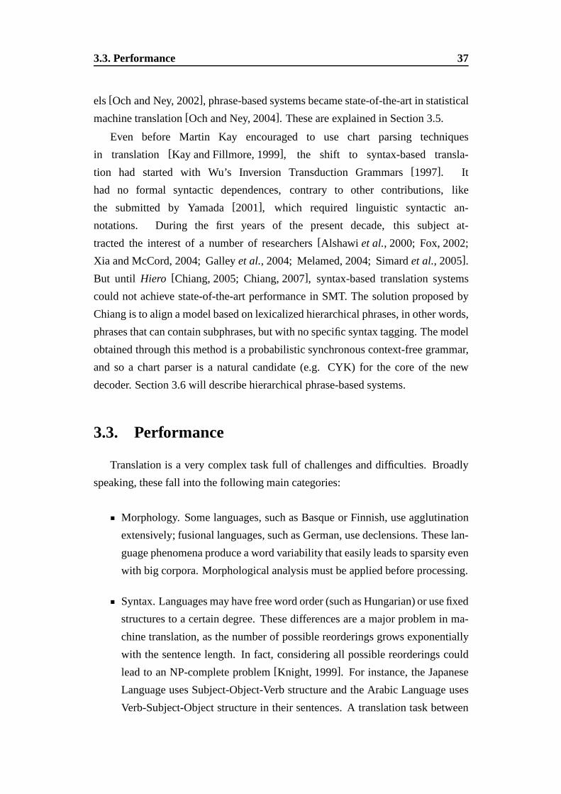
3.3. Performance 37
els[Och and Ney, 2002], phrase-based systems became state-of-the-art in statistical
machine translation[Och and Ney, 2004]. These are explained in Section 3.5.
Even before Martin Kay encouraged to use chart parsing techniques
in translation [Kay and Fillmore, 1999], the shift to syntax-based transla-
tion had started with Wu’s Inversion Transduction Grammars[1997]. It
had no formal syntactic dependences, contrary to other contributions, like
the submitted by Yamada[2001], which required linguistic syntactic an-
notations. During the first years of the present decade, thissubject at-
tracted the interest of a number of researchers[Alshawiet al., 2000; Fox, 2002;
Xia and McCord, 2004; Galleyet al., 2004; Melamed, 2004; Simardet al., 2005].
But until Hiero [Chiang, 2005; Chiang, 2007], syntax-based translation systems
could not achieve state-of-the-art performance in SMT. Thesolution proposed by
Chiang is to align a model based on lexicalized hierarchicalphrases, in other words,
phrases that can contain subphrases, but with no specific syntax tagging. The model
obtained through this method is a probabilistic synchronous context-free grammar,
and so a chart parser is a natural candidate (e.g. CYK) for thecore of the new
decoder. Section 3.6 will describe hierarchical phrase-based systems.
3.3. Performance
Translation is a very complex task full of challenges and difficulties. Broadly
speaking, these fall into the following main categories:
Morphology. Some languages, such as Basque or Finnish, use agglutination
extensively; fusional languages, such as German, use declensions. These lan-
guage phenomena produce a word variability that easily leads to sparsity even
with big corpora. Morphological analysis must be applied before processing.
Syntax. Languages may have free word order (such as Hungarian) or use fixed
structures to a certain degree. These differences are a major problem in ma-
chine translation, as the number of possible reorderings grows exponentially
with the sentence length. In fact, considering all possiblereorderings could
lead to an NP-complete problem[Knight, 1999]. For instance, the Japanese
Language uses Subject-Object-Verb structure and the Arabic Language uses
Verb-Subject-Object structure in their sentences. A translation task between

38 Chapter 3. Machine Translation
Japanese and Arabic would require to move the verb from the beginning of
the sentence to the end or vice versa.
Semantics. The semantic problem is two-fold:
• Word sense. Words, idioms and even proper names depend on thecon-
text, which in most cases allows to disambiguate correctly.
• Sublanguages. It is not the same to translate religious texts than newspa-
pers. Novels, textbook and legal documents fall into different domains.
This affects vocabulary (i.e. consider technical versus poetic texts), style
(passive versus active voice), etcetera. Unfortunately, amachine trans-
lation system that works reasonably well for one sublanguage will not
necessarily work well for another.
Phonetics. Names often require transliteration, rather than translation, and
thus it is required to obtain an orthographic solution for the phonetically clo-
sest pronunciation of a foreign word[Menget al., 2001].
These problems account for the enormous ambiguity involvedin a translation
task and hence the difficulty to obtain reasonable quality, specifically in certain lan-
guage pairs such as Chinese-to-English1. But even so, there is yet another very
serious problem in this task: how can we measure quality? Automatic metrics de-
pend on (at least ) one reference. But this represents a smallsubset of all the possible
correct translations to a given source sentence, as even expert humans do not trans-
late in the same way. So it is not easy to ensure that an automatic metric correlates
to human judgements. There is an ongoing discussion in the research community
over automatic and human metrics, both to be introduced in the next subsections.
3.3.1. Automatic Evaluation Metrics
Many automatic metrics contrasting hypotheses against oneor more references
have been proposed to evaluate translation tasks, such as Word Error Rate, Posi-
tion Independent Rate, BLEU[Papineniet al., 2001], TER[Snoveret al., 2006] or
GTM [Turianet al., 2003] among others. But almost ten years after its conception,
1Not to forget the availability of parallel corpora, which depends on the interest of the communityor funders. For instance, there are loads of data for Chinese-to-English, but it would probably be verydifficult to obtain even a few hundreds of sentences for a Japanese-Galician translation system.
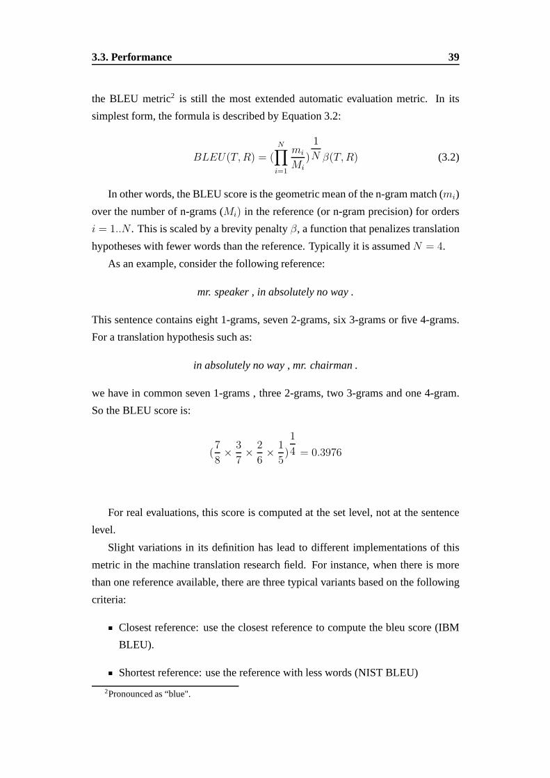
3.3. Performance 39
the BLEU metric2 is still the most extended automatic evaluation metric. In its
simplest form, the formula is described by Equation 3.2:
BLEU(T,R) = (N∏
i=1
mi
Mi)
1
N β(T,R) (3.2)
In other words, the BLEU score is the geometric mean of the n-gram match (mi)
over the number of n-grams (Mi) in the reference (or n-gram precision) for orders
i = 1..N . This is scaled by a brevity penaltyβ, a function that penalizes translation
hypotheses with fewer words than the reference. Typically it is assumedN = 4.
As an example, consider the following reference:
mr. speaker , in absolutely no way .
This sentence contains eight 1-grams, seven 2-grams, six 3-grams or five 4-grams.
For a translation hypothesis such as:
in absolutely no way , mr. chairman .
we have in common seven 1-grams , three 2-grams, two 3-grams and one 4-gram.
So the BLEU score is:
(7
8×
3
7×
2
6×
1
5)
1
4 = 0.3976
For real evaluations, this score is computed at the set level, not at the sentence
level.
Slight variations in its definition has lead to different implementations of this
metric in the machine translation research field. For instance, when there is more
than one reference available, there are three typical variants based on the following
criteria:
Closest reference: use the closest reference to compute thebleu score (IBM
BLEU).
Shortest reference: use the reference with less words (NISTBLEU)
2Pronounced as “blue".

40 Chapter 3. Machine Translation
Average reference: Once computed for all the references, compute the mean.
BLEU has received many criticisms in these years. Among them, in one inter-
esting paper written by Callison-Burch and Osborne[2006] there is an extensive
discussion concerning the use of BLEU for Machine Translation, and concrete ex-
amples are shown in which it does not correlate with human judgement. One impor-
tant reason for this could be that while maximum entropy systems use BLEU as the
optimization metric, rule-based machine translations systems do not. In conclusion,
it is suggested that the BLEU score should be used restrictedto several scenarios,
as for instance a comparison between very similar systems.
Many other automatic metrics have been proposed along this decade to over-
throw BLEU. For instance, theNIST metric [Doddington, 2002] is a variant of
BLEU that assigns different value to each matching n-gram according to informa-
tion gain statistics. It has less sensitivity to brevity penalty. Scoring range goes
from 0 to ∞. METEOR[Banerjee and Lavie, 2005] is a harmonic mean of uni-
gram precision and recall. Other metrics areORANGE[Lin and Och, 2004], and
ROUGE[Lin, 2004].
Another one commonly used nowadays is the Translation Edit Rate metric
(TER), a variant of the well known word error rate (WER) metric, which counts
the minimum number of insertions, deletions and substitutions needed to go from a
candidate sentence to the reference sentence. TER also counts shifts of continuous
blocks in the hypothesis.
TER(T,R) =Ins+Del + Sub+ Shft
N(3.3)
For the previous example, it would be required to shift 4 times and make one
substitution. So the TER score is:
0 + 0 + 1 + 4
8= 0.625
3.3.2. Human Evaluation Metrics
Once the references have been defined for a given test set, automatic evalu-
ations are easy and quite cheap. The main problem with automatic metrics is
their correlation to human evaluation. In contrast, human evaluation is a dif-
ficult challenge, due to the intrinsic subjectiveness of thetask. Despite seve-
ral different attempts (for instance, binary contrast preference and preference

3.4. Statistical Machine Translation Systems 41
reranking[Callison-Burchet al., 2008]) traditionally human judgement has focused
mainly on two aspects:
Fluency. Indicates naturalness of the sentence to a native speaker.
Adequacy. Indicates correctness of a candidate sentence compared toa refer-
ence.
Generally these kind of evaluations use trivial grades (e.g. from 1 to 5 ). De-
ciding the grade that applies for each case is itself a very subjective exercise, which
further complicates trying to establish common criteria for a group of judges.
One interesting alternative in the machine translation literature consists of us-
ing HTER [Snoveret al., 2006; Snoveret al., 2009], which is based on the TER
formula presented in Equation 3.3 and thus shares its advantages and weakness;
it has been claimed that used adequately it correlates better to human judgement
than BLEU[Callison-Burch, 2009]. The idea is that a human edits the translated
sentence from the system in such way that the edited version must be correct and
contain the complete original meaning from the source sentence. Actually, this idea
is applicable to any other automatic metric (i.e. Human METEOR, Human BLEU,
etcetera).
3.4. Statistical Machine Translation Systems
Equation 3.1 expresses that the translation problem has twobasic components,
being the first a translation model and the second one a language model. The trans-
lation model assigns weights for any source word translatedto any target word,
whereas the language model assigns better weights to more fluent hypotheses3. A
decoder will output translation hypotheses with final weights corresponding to the
contributions of both the translation and the language model. We expect the trans-
lation hypothesis with the best weight to be the best translation. Nowadays state-of-
the-art systems tend to use maximum entropy frameworks, which allow to represent
the translation model as a log-combination of models or features.
In order to learn these models, it is required two kind of corpora. For the lan-
guage model a typical monolingual corpus is enough. For the translation model, it
3So this fundamental equation has itself a correspondence with adequacy (translation model) andfluency (language model).
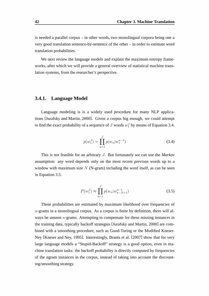
42 Chapter 3. Machine Translation
is needed a parallel corpus – in other words, two monolingualcorpora being one a
very good translation sentence-by-sentence of the other – in order to estimate word
translation probabilities.
We next review the language models and explain the maximum entropy frame-
works, after which we will provide a general overview of statistical machine trans-
lation systems, from the researcher’s perspective.
3.4.1. Language Model
Language modeling is is a widely used procedure for many NLP applica-
tions [Jurafsky and Martin, 2000]. Given a corpus big enough, we could attempt
to find the exact probability of a sequence ofJ wordswJ1 by means of Equation 3.4.
p(wJ1 ) =
J∏
n=1
p(wn|wn−11 ) (3.4)
This is not feasible for an arbitraryJ . But fortunately we can use theMarkov
assumption: any word depends only on the most recent previous words up to a
window with maximum sizeN (N-gram) including the word itself, as can be seen
in Equation 3.5.
P (wJ1 ) ≈
J∏
n=1
p(wn|wn−1n−N+1) (3.5)
These probabilities are estimated by maximum likelihood over frequencies of
n-grams in a monolingual corpus. As a corpus is finite by definition, there will al-
ways be unseenn-grams. Attempting to compensate for these missing instances in
the training data, typically backoff strategies[Jurafsky and Martin, 2000] are com-
bined with a smoothing procedure, such as Good-Turing or theModified Kneser-
Ney [Kneser and Ney, 1995]. Interestingly, Brants et al.[2007] show that for very
large language models a “Stupid-Backoff" strategy is a goodoption, even in ma-
chine translation tasks: the backoff probability is directly computed by frequencies
of the ngram instances in the corpus, instead of taking into account the discount-
ing/smoothing strategy.

3.4. Statistical Machine Translation Systems 43
3.4.2. Maximum Entropy Frameworks and Minimum Error
Training
By using log-linear combination we can combine a set of featuresfm(s, t) that
contribute differently according to weightsλm, as described by Equation 3.6.
tI1 = argmax
M∑
m=1
λm fm(sJ1 , t
I1)
(3.6)
Weights are optimized, for instance with Minimum Error Training [Och, 2003],
using as the objective function an automatic metric such as BLEU. The strategy
provides significant gains over uniform weights. Typical features used to train a
maximum entropy model in this research field are translationmodels in both direc-
tions, the word penalty (to compensate language models tendency to assign better
scores to shorter sentences), a phrase or rule insertion penalty, lexical features4 and,
of course, the target language model. Many contributions inthe research field are
based on the design of new features acting assoft constraintsto the model. The
Minimum Error Training procedure is limited in the amount offeatures it can han-
dle. To overcome this limitation, the Margin Infused Relaxed Algorithm has been
proposed for this optimization task[Chianget al., 2009].
3.4.3. Model Estimation and Optimization
Statistical Machine Translation models are estimated overlarge collections of
data, including at least a parallel and a monolingual corpus. Most of the transla-
tion models are defined by the kind of translation unit used: these could be words,
sequences of words or more complex syntactically based units. In any case, once
the models have been calculated an optimization strategy isrequired to combine
adequately all these models into one unique global model. Only then we can test
the performance of our system. Summing up, the Statistical Machine Translation
problem has two differentiated parts:
1. Models Estimation
2. Optimization
Figure 3.2 depicts a general overview of the models estimation. In general, two
kind of corpora are used for this purpose: parallel (alignedsentence-by-sentence)4Based on IBM model 1.

44 Chapter 3. Machine Translation
Figure 3.2: Model Estimation.
and (target) monolingual, which we assume here to be concordantly tokenized. The
target language model is estimated from both the target sideof the parallel corpus
and the monolingual corpus. From the parallel corpus we haveto estimate the trans-
lation units. Which kind of translation units we are considering to extract is related
to the kind of statistical machine system we are actually using to decode. In state-of-
the-art systems the translation unit is typically more complex than aligned words.
It should be noted too that many models or features are uniquely determined by
these translation units (such as the forward and backward translation models). Nev-
ertheless, information from word alignments is used in order to build these more
complex translation units, so word alignments are typically extracted in a first pass.
The general procedure will be described in Section 3.4.4.
Before we can test our system we must find a set of weights that will balance
our models in the best way possible. For this the typical solution is Minimum Error
Training[Och, 2003]. The main idea is the following: using an initial set of weights,
we perform a translation over a development set. By means of an automatic metric,
the optimization looks for a new set of weights for which it expects the system to
perform better. This expectation must be tested with a new translation, which in turn
leads to a new optimization and so on until the optimization converges according to
a certain criterion (typically related to the BLEU score). As shown in Figure 3.3,
once the optimization is over we can test the system with the final weights, using

3.4. Statistical Machine Translation Systems 45
automatic and/or human metrics.
Figure 3.3: Parameter optimization and test translation.
3.4.4. Word Alignment and Translation Unit
A key characteristic of actual Machine Translation systemsis the translation
unit, which determines not only how the translation must be performed, but it also
requires a special extraction algorithm from the parallel corpora (with the corre-
sponding weights). The most naive system would use only aligned words as the
translation unit. An example of word alignments is shown in Figure 3.4.
Figure 3.4: An example of word alignments.
The word alignment mathematical process is described by Brown et al.[1990;
1993]. The basic idea consists of defining a hidden variablea(s, t) to model the
alignment between sentences, so we can extend the translation model from Equa-
tion 3.1 into Equation 3.7.

46 Chapter 3. Machine Translation
p(s|t) =∑
a
p(s, a|t) (3.7)
In other words, given a target sentencet the global probability of having trans-
lated from a source sentences is the sum of the probabilities restricted to each
possible set of alignments that allow this particular translation. For each alignment,
considering that we haveJ source words andI target words, i.e.s = sJ1 , a = aJ1
andt = tI1, theexactalignment equation is defined by:
p(s, a|t) = p(J |t)J∏
j=1
p(aj |aj−11 , sj−1
1 , J, t)p(sj|aj1, s
j−11 , J, t) (3.8)
From a generative point of view, Equation 3.8 suggests that if we had to translate
from target to source we would first decide the size of the source sentence, then
create the next alignment from a target word and finally create the next source word.
Equation 3.8 is actually not tractable for a fully automaticprocess. But as-
sumptions applied to Equation 3.8 lead to a series of models of growing complexity
commonly referred to in the literature as theIBM models. Five were proposed in
this influential paper by Brown et al.[1993]:
Model 1 is the simplest of all. Considers that alignment probabilities follow
a uniform distribution.
Model 2 makes the alignments dependent of position in the source. Vogel et
al. refined this model into the so-calledHMM alignment model[1996], which
adds a first order dependency on the alignment of the previousword.
Model 3 introducesfertility i.e. allows a target word to generate more than
one source word with a certain probability.
Models 4 and 5 refine fertility.
These models can be estimated using the Expectation-Maximization algo-
rithm [Dempsteret al., 1977]. As each model is actually a refinement of the pre-
vious one, the parameters extracted from model 1 is used to estimate model 2 and
so on, in order to ensure convergence. There are tools freelyavailable that esti-
mate the word alignments, such as GIZA++[Och and Ney, 2000] and the MTTK
toolkit [Deng and Byrne, 2006], which estimates word alignments using a word-to-
phrase model.

3.4. Statistical Machine Translation Systems 47
Word alignments have a direction (i.e. word links are in practice 1-to-N in
each direction). In order to calculate the translation unitmodels, word align-
ments in both directions are required. To do this, although several strategies have
been proposed and discussed in the SMT literature (i.e. union, intersection, re-
fined[Och and Ney, 2003] and grow-final-diag[Koehnet al., 2007] ), the union of
both alignments is typically applied.
During this decade more complex translation units have beenproposed success-
fully:
Phrases: sequences of consecutive words. Used by phrase-based models such
as TTM[Blackwoodet al., 2008] and Moses[Koehnet al., 2007]. These will
be explained in Section 3.5.
Tuples: a subset of phrases. Used by n-gram based models such
as Marie [Cregoet al., 2005; Mariñoet al., 2006] inspired on a trans-
lation system based on finite-state transducers developed by Casacu-
berta[Casacuberta, 2001; Casacuberta and Vidal, 2004]. See Section 3.5.2.
Syntactic phrases: an extension to phrases. These may contain gaps to be
filled with other phrases in a recursive fashion. These gaps may have linguis-
tically syntactic meaning or not. The phrases for the lattercase usually are re-
ferred to ashierarchical phrasesor hiero phrases; and are widely used within
hierarchical phrase-based decoders[Chiang, 2007; Iglesiaset al., 2009c]. Hi-
ero phrases will be introduced in Section 3.6 and expanded inChapter 4.
Other syntactic units. In contrast to the string-to-stringtranslation units de-
scribed before, it has been proposed several SMT systems using more com-
plex translation units involving trees and operations withtrees, either on
source or target. These systems, not having yet reached state-of-the-art re-
sults for large scale translation tasks, promise new strands of research in
the near future. It is worth citing here tree-to-tree modelssuch as data ori-
ented translation[Poutsma, 2000], translation with synchronous tree adjoin-
ing grammars[Shieber, 2007] and with packed forests[Liu et al., 2009]. Ya-
mada and Knight[2001], Galley et al.[2006], Graehl and Knight[2008],
Nguyen et al.[2008] and Zhang et al.[2009] have been working on tree-to-
string models.

48 Chapter 3. Machine Translation
In general, translation units are extracted using the word alignments previously
obtained with IBM models 1-5, with symmetrization, although it should be noted
that alternative methods have been proposed in the literature, such as word align-
ments based on Stochastic Inversion Transduction Grammars[Saers and Wu, 2009].
The translation model to use in each case will be defined by relative counts of these
translation units instead of the word alignment probabilities. Tuples, phrases and
hierarchical phrases will be reviewed in more detail in the following sections.
3.5. Phrase-Based systems
In the context of Statistical Machine Translation, phrases[Ochet al., 1999;
Koehnet al., 2003] are simply bitext sequences of words. The phrase alignment
process departs from the word alignments and builds every possible bitext sequence
up to a maximum number of source wordsPW , provided that it containscom-
pletelyall the word alignments. Figure 3.5 shows the phrases extracted from the
word alignments in Figure 3.4.
comida # foodchina # chinese
quisiéramos # would likequisiéramos # we would like
comprar # to buyquisiéramos comprar # would like to buy
quisiéramos comprar # we would like to buycomida china # chinese food
comprar comida china # to buy chinese foodquisiéramos comprar comida china # would like to buy chinesefood
quisiéramos comprar comida china # we would like to buy chinese food
Figure 3.5: An example of phrases extracted from alignmentsin Figure 3.4.
For instance, Figure 3.5 shows all the possible phrases extracted from word
alignments for a Spanish-English bi-sentence. In this example, it is not possible to
extract the phrase
quisiéramos comprar # would like to
becausecomprar is aligned to a word that is not in the phrase (buy). On the other
hand, ifPW = 3 then the phrase extraction algorithm would disallow:
quisiéramos comprar comida china# we would like to buy chinese food
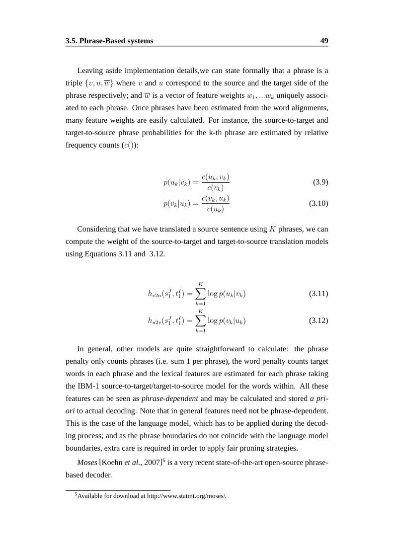
3.5. Phrase-Based systems 49
Leaving aside implementation details,we can state formally that a phrase is a
triple v, u, w wherev andu correspond to the source and the target side of the
phrase respectively; andw is a vector of feature weightsw1, ...wk uniquely associ-
ated to each phrase. Once phrases have been estimated from the word alignments,
many feature weights are easily calculated. For instance, the source-to-target and
target-to-source phrase probabilities for the k-th phraseare estimated by relative
frequency counts (c()):
p(uk|vk) =c(uk, vk)
c(vk)(3.9)
p(vk|uk) =c(vk, uk)
c(uk)(3.10)
Considering that we have translated a source sentence usingK phrases, we can
compute the weight of the source-to-target and target-to-source translation models
using Equations 3.11 and 3.12.
hv2u(sJ1 , t
I1) =
K∑
k=1
log p(uk|vk) (3.11)
hu2v(sJ1 , t
I1) =
K∑
k=1
log p(vk|uk) (3.12)
In general, other models are quite straightforward to calculate: the phrase
penalty only counts phrases (i.e. sum 1 per phrase), the wordpenalty counts target
words in each phrase and the lexical features are estimated for each phrase taking
the IBM-1 source-to-target/target-to-source model for the words within. All these
features can be seen asphrase-dependentand may be calculated and storeda pri-
ori to actual decoding. Note that in general features need not bephrase-dependent.
This is the case of the language model, which has to be appliedduring the decod-
ing process; and as the phrase boundaries do not coincide with the language model
boundaries, extra care is required in order to apply fair pruning strategies.
Moses[Koehnet al., 2007]5 is a very recent state-of-the-art open-source phrase-
based decoder.
5Available for download at http://www.statmt.org/moses/.

50 Chapter 3. Machine Translation
3.5.1. TTM
The Transducer Translation Model(TTM) is a phrase-based SMT system im-
plemented with Weighted Finite-State transducers using standard WFST operations
with the Openfst library[Allauzenet al., 2007]. It is formulated as a generative
source-channel model for phrase-based translation in which a series of stochastic
transformations of a target sentence (via translation, reordering, and so on) lead to
a source sentence. Note that in this model the source (English) and target (foreign)
are swapped. Anad hocdecoder is not needed in this case, as the model is simply
designed as a composition of the following models/transducers.
G: Contains the source language model implemented as a finite-state automa-
ton using failure transitions for exact implementation.
W : The unweighted source phrase segmentation, maps phrases to words.
R: Phrase translation and reordering models.
Φ: Target phrase insertion6
Ω: The unweighted target phrase segmentation. It maps from words to
phrases.
Word and Phrase Penalties.
If T contains the input sentence (or input lattice) we wish to translate, then the
translation lattice is obtained via WFST composition:
L = G W R Φ Ω T (3.13)
Modularity is one of its best advantages, as each model is easy to work with
separately, and adding new models is fairly straightforward. For instance,R itself
is a composition of a basic phrase translation model with a reordering model, such
as Maximum-Jump-1 (MJ1)[Kumar and Byrne, 2005], that allows phrases to jump
either left or right to a maximum distance of one phrase.

3.5. Phrase-Based systems 51
quisiéramos # would likecomprar # to buy
comida china # chinese food
Figure 3.6: An example of tuples extracted from alignments inf Figure 3.4.
3.5.2. The n-gram-based System
This system models the translation problem within the maximum-entropy
framework as a language model of a particular bilanguage composed of translation
units (tuples), and thus theMarkovassumption is used to simplify the calculation of
weights, as shown in Equation 3.14.
p(T, S) =
K∏
k=1
p((t, s)k|(t, s)k−N+1, ..., (t, s)k−1) (3.14)
Tuples, which are a subset of phrases, are extracted from many-to-many word
alignments according to the following restrictions[Cregoet al., 2004]:
Tuples are the set of shortest phrases for a monotonic segmentation.
A unique, monotonous segmentation of each sentence pair is produced.
No word in a tuple is aligned to words outside of it.
No smaller tuples can be extracted without violating the previous constraints
Tuples with empty source sides are not allowed.
Figure 3.6 shows the tuple extraction for a pair of sentenceswith word align-
ments. In contrast to phrase extraction, the tuple extraction does not have a risk of
explosion and thus there is no need of controlling the size ofthe tuples. In general
this should benefit translation for similar languages, as tuples are able to handle
short reorderings defined by the word alignments within. Fordistant reorderings,
tuples big enough to contain these word reorderings are required. Hence, tuple
sparseness makes the system more likely to fail[Mariñoet al., 2006].
This strategy requires a special decoder. There is an open-source tool avail-
able namedMarie7 [Cregoet al., 2005], that decodes monotonically using a beam-
search with pruning and hypothesis recombination. Pruningis applied to translation
6This corresponds to phrase deletions from source (foreign)to target (English)7Available for download at http://gps-tsc.upc.es/veu/soft/soft/marie/.

52 Chapter 3. Machine Translation
hypotheses for the same number of source words to ensure a fair competition be-
tween hypotheses.
3.6. Syntactic Phrase-based systems
Syntactic phrase-based systems extend the definition of thephrase into a quadru-
pleγ, α, w,∼. Now γ andα are sequences of words with an arbitrary number of
gaps8, and∼ is a bijective function that maps gaps between source (γ) and target
(α). These gaps point recursively to other phrases, synchronized across both lan-
guages. Gaps could have a syntactic meaning, i.e. phrases underlying actually yield
a syntactic function (NP, VP, etc). If they do not, we call these phraseshierarchical.
Consequently, the systems that use these kind of phrases fall into the category of
hierarchical phrase-based systems. Figure 3.7 shows the hierarchical phrases cor-
responding to the word alignments in Figure 3.4. Gaps for hierarchical systems are
typically indicated with the capital letterX. Estimating hierarchical models is very
similar to estimating phrase-based models as we still have the language model and
a set of weights that are uniquely defined by the translation units.
comida # food...
quisiéramos comprar comida china # we would like to buy chinese foodX china # chineseXX china #X food
quisiéramosX # would likeXquisiéramosX # we would likeX
X comprar #X to buyX1 comprarX2 china #X1 to buy chineseX2
...
Figure 3.7: An example of hierarchical phrases extracted from alignments in Fig-ure 3.4.
The hierarchical phrase-based models were introduced by Chiang[2005] using
synchronous context-free grammars as the framework basis for the translation units.
The decoder typically involves at least a monolingual context-free parser with a
second pass to build the translation search space, althoughChiang also proposed
the use of a bilingual parser, hence constructing the translation search space in only
one pass. Hierarchical decoding will be explained in more detail in Chapter 4.
8Typically limited up to two gaps.

3.7. Reranking and System Combination 53
3.7. Reranking and System Combination
It is not uncommon nowadays in natural language processing to rerank or
rescore in a second stage the lattice or n-best lists of hypotheses produced by a
system. Statistical machine translation reranking strategies have been described
in [Shenet al., 2004; Ochet al., 2004] for oracle studies, and implemented for in-
stance with lattices by Blackwood et al.[2008] for large scale translation tasks. One
practical reason to do this is typically that the decoder itself depending on its partic-
ular architecture and hardware restrictions can handle reasonably language models
up to a given maximum threshold size9. Once the decoder has finished, the list of
hypotheses are rescored by taking away the language model costs assigned by the
decoder and reapplying language model costs estimated overlarge-scale corpora,
and containing higher-ordern-grams.
Another widespread strategy in natural language processing is to combine the
output of many decoders and choose the best hypotheses according to certain crite-
ria, relying on the fact that, appropriately done, it will take advantage in many cases
of the strengths of each individual system avoiding their weaknesses. This proce-
dure is calledsystem combination. In particular, it has become a notable current
trend in statistical machine translation.
For instance, Minimum Bayes risk decoding is widely used to rescore and
improve hypotheses produced by individual systems[Kumar and Byrne, 2004;
Trombleet al., 2008; de Gispertet al., 2009b]. More aggressive system combi-
nation techniques that synthesize entirely new hypothesesfrom those of con-
tributing systems can give even greater translation improvements[Simet al., 2007;
Rostiet al., 2007; Fenget al., 2009]. It is now commonplace to note that even the
best available individual SMT system can be significantly improved upon by such
techniques. In turn, both reranking and system combinationburden the underlying
SMT systems with the requirement of producing large collections of candidate hy-
potheses that are simultaneously diverse and of good quality, instead of the single
1-best hypothesis considered for performance evaluation.
9As a good example of how using the language model affects speed, Chiang[2007] contrasts ahierarchical system that does not apply language models (the -LM decoder) with two other systemsthat use only a3-gram language model. The difference in terms of speed (and of course performance)is quite notable.

54 Chapter 3. Machine Translation
3.8. WFSTs for Translation
There is extensive work in using Weighted Finite-State Transducers for machine
translation. For instance, Bangalore and Riccardi[2002] present the translation
task as a composition of a translation lattice with a reordering lattice, although no
performance in terms of BLEU scores are presented in this paper. Casacuberta
and Vidal [2004] describe inference techniques for weighted transducers applied
to machine translation. To overcome reordering limitations, Matusov et al.[2005]
propose source sentence word reordering in training and translation.
Kumar et al. develop the Translation Template Model[2006], a full phrase-
based translation system with constrained phrase-based reordering, yielding re-
spectable performance on large bitext translation tasks. This system has also been
used successfully for speech translation[Mathias and Byrne, 2006].
Graehl and Knight[2008] motivate the usage of tree-to-string transducers.
Tromble et al.[2008] develop a lattice implementation of a Minimum-Bayes Risk
system, used for rescoring and system combination, with consistent gains in perfor-
mance.
3.9. Conclusions
The Machine Translation field is very active nowadays and attracts the interest
of many researchers, as can be seen by the number of contributions to important
conferences and journals10 or various workshops for MT shared tasks11. In this
chapter we have presented a very brief overview of this field.After a historic review
and discussing the problem of performance, we have described the basic framework
for most of the state-of-the-art SMT systems today. The translation unit is key to the
design of both the search space and the decoding algorithm. As such, it determines
the kind of SMT system. Many features depend uniquely on the translation unit;
other features have other dependencies. Among the latter ones, a good example
is the language model. Hierarchical phrase-based decodersare based on a transla-
tion unit (hierarchical phrases) conceived as variant of other translation units called
“phrases" in which gaps are now also considered instead of words alone. In the next
10For instance, see the ACL conferences and journal papers, http://aclweb.org/anthology-new/.11For instance, the NIST (http://www.itl.nist.gov/iad/mig/tests/mt/) and the ACL workshop
(http://www.statmt.org/wmt09/).

3.9. Conclusions 55
chapter we get into the details of a special kind of hierarchical decoder based on the
well known hypercube pruning technique.


Chapter 4Hierarchical Phrase-based Translation
Contents4.1. Introduction . . . . . . . . . . . . . . . . . . . . . . . . . . . 57
4.2. Hierarchical Phrase-Based Translation . . . . . . . . . . . . 58
4.3. Hypercube Pruning Decoder . . . . . . . . . . . . . . . . . . 60
4.4. Two Refinements in the Hypercube Pruning Decoder . . . . 66
4.5. A Study of Hiero Search Errors in Phrase-Based Translation 69
4.6. Related Work . . . . . . . . . . . . . . . . . . . . . . . . . . 71
4.7. Conclusions . . . . . . . . . . . . . . . . . . . . . . . . . . . . 74
4.1. Introduction
In this chapter we introduce hierarchical phrase-based translation. After a gen-
eral overview in Section 4.2, we get into the details of our hypercube pruning de-
coder1 in Section 4.3 using the k-best algorithm[Chiang, 2007]. We describe tech-
niques to reduce memory usage and search errors in hierarchical phrase-based trans-
lation in Section 4.4. Memory usage can be reduced in hypercube pruning through
smart memoization, and spreading neighbourhood exploration can be used to re-
duce search errors. In Section 4.5, we show that search errors still remain even
when implementing simple phrase-based translation due to the use of k-best lists.
We discuss this issue with a contrastive experiment, for which we use as a golden
1Although the original name iscube pruning, we will use the prefixhyper- as the algorithmactually builds hypercubes of different orders to prune.

58 Chapter 4. Hierarchical Phrase-based Translation
reference another phrase-based system. After reviewing inSection 4.6 the state of
the art for hierarchical phrase-based translation, we conclude.
4.2. Hierarchical Phrase-Based Translation
Hierarchical phrase-based translation[Chiang, 2005] has emerged as one of the
dominant current approaches to statistical machine translation. Hiero translation
systems incorporate many of the strengths of phrase-based translation systems, such
as feature-based translation and strong target language models, while also allowing
flexible translation and movement based on hierarchical rules extracted from aligned
parallel text. The approach has been widely adopted and reported to be competitive
with other large-scale data driven approaches, e.g.[Zollmannet al., 2008].
Basically, Hiero systems use phrase-based rules equivalent to traditional phrase-
based translation and hierarchical rules that model reordering, guided by a parser:
the underlying idea is that both languages have very similar‘syntactic’ trees. Pars-
ing may be monolingual (i.e. using rules over the source language) or bilingual
(synchronous rules for both the source and the target language). If the parsing is
bilingual, target hypotheses are built at the parsing stage, whereas a monolingual
parse delays this hypotheses generation to a second step. Inboth cases, hypotheses
generation must be guided by the target language model.
As introduced in Section 3.6, the translation units for the hierarchical model,
which we callhiero phrases, can be seen as an extension to normal phrases. As
such, they can be defined as a quadrupleγ, α, w,∼, with γ andα mixing words
and gaps, whereas∼ relates gaps between source and target. The hiero phrase ex-
traction procedure is a heuristic method that departs from the word alignments. In
first place, the usual phrases〈sji , tj′
i′ 〉 are extracted. Then, for each candidate hiero
phrase it is inspected whether there exists a subsequence ofaligned terminals in
both source and target that correspond to any phrase〈sji , tj′
i′ 〉. If this is the case,
the terminal subsequence in both source and target are replaced by a non-terminal
X. In other words, if we have a candidate〈γ1sjiγ2, α1t
j′
i′α2〉 and we have derived
the phrase〈sji , tj′
i′ 〉, then we can derive〈γ1Xkγ2, α1Xkα2〉. This candidate is added
and the search for new candidates keeps going until no more hiero phrases can be
derived. This extraction obeys the following constraints to avoid excessive redun-
dancy[Chiang, 2007]:

4.2. Hierarchical Phrase-Based Translation 59
1. Unaligned words are not allowed at the edge of (hierarchical) phrases.
2. Initial phrases are limited to a length of 10 words on either side.
3. Hierarchical rules with up to two non-terminals are allowed.
4. Non-terminals on the source side are not allowed to be adjacent.
5. Rules are limited on the source side to a string of five elements, consider-
ing an element as either a non-terminal or a subsequence of terminals (see
Chapter 5).
6. Rules must be lexicalized, i.e. they must contain at leastone pair of aligned
words.
In brief, the model derived in this way builds on phrase-based systems in the
sense that it takes the advantage of their local word reordering power. But even
more, it provides special lexicalized phrases with gaps that must point to other
phrases (possibly pointing to other phrases, etcetera), thus yielding a very pow-
erful reordering model. It should be noted that in principleit is possible to use
gap phrases with non hierarchical systems, i.e. in extendedphrase-based sys-
tems[Galley and Manning, 2008] or tuple-based systems[Crego and Yvon, 2009].
On the other hand, only hierarchical decoders are capable ofhandling the full power
conveyed by these rules, expressed in a special type of bilingual grammars that
transduce context-free grammars, to be explained in Section 4.3.2. Chiang intro-
duced threeHiero strategies[Chiang, 2007]:
-LM decoder: The system translates in three steps. The first step is devoted to
parsing the source sentence with a modified CYK algorithm, whilst the second
step traverses the derivations in order to build different translation hypotheses.
For this, Chiang describes his k-best algorithm with memoization. Language
Model is incorporated via rescoring as a third step. As thereis pruning in
search without the language model, it yields the worst performance, although
it is also the fastest system.
Intersection decoder: The slowest solution, as it builds translations in one
single pass during parsing, and therefore is effectively using a grammar with
rules that bind both source and target phrases. The languagemodel is ‘inter-
sected’ with the grammar, inspired by Wu’s similar idea of combining brack-
eting transduction grammars with bigram models[1996].
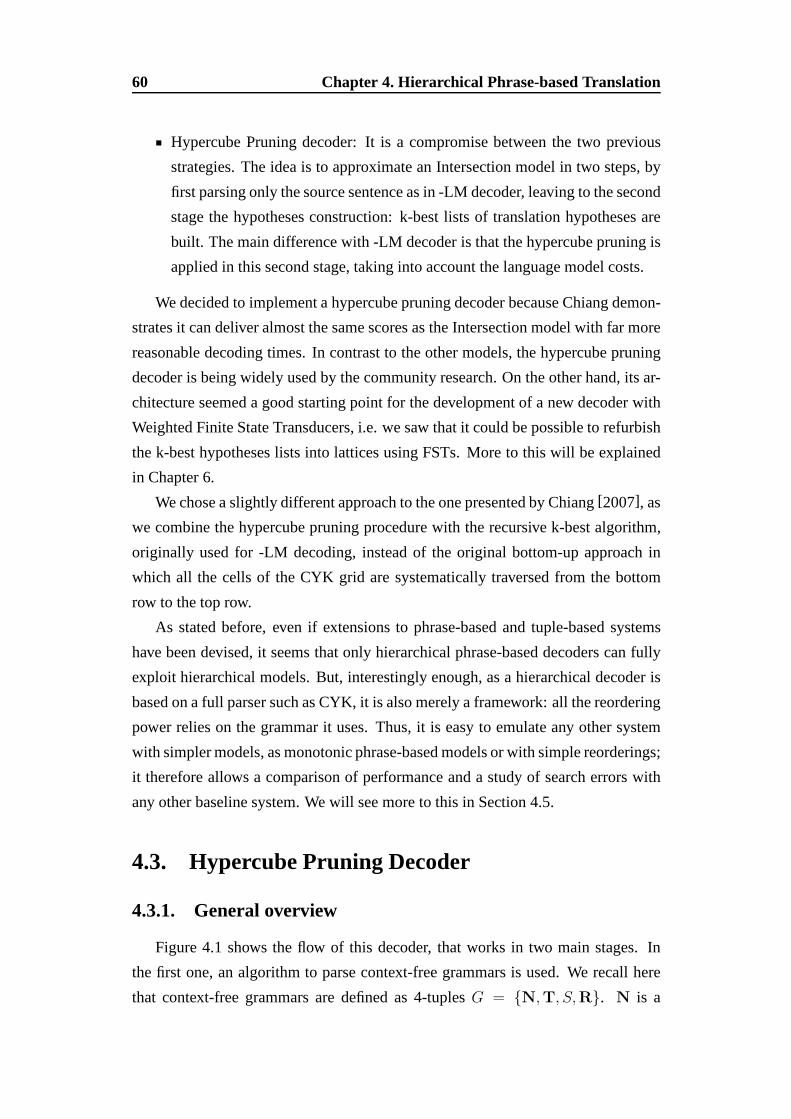
60 Chapter 4. Hierarchical Phrase-based Translation
Hypercube Pruning decoder: It is a compromise between the two previous
strategies. The idea is to approximate an Intersection model in two steps, by
first parsing only the source sentence as in -LM decoder, leaving to the second
stage the hypotheses construction: k-best lists of translation hypotheses are
built. The main difference with -LM decoder is that the hypercube pruning is
applied in this second stage, taking into account the language model costs.
We decided to implement a hypercube pruning decoder becauseChiang demon-
strates it can deliver almost the same scores as the Intersection model with far more
reasonable decoding times. In contrast to the other models,the hypercube pruning
decoder is being widely used by the community research. On the other hand, its ar-
chitecture seemed a good starting point for the developmentof a new decoder with
Weighted Finite State Transducers, i.e. we saw that it couldbe possible to refurbish
the k-best hypotheses lists into lattices using FSTs. More to this will be explained
in Chapter 6.
We chose a slightly different approach to the one presented by Chiang[2007], as
we combine the hypercube pruning procedure with the recursive k-best algorithm,
originally used for -LM decoding, instead of the original bottom-up approach in
which all the cells of the CYK grid are systematically traversed from the bottom
row to the top row.
As stated before, even if extensions to phrase-based and tuple-based systems
have been devised, it seems that only hierarchical phrase-based decoders can fully
exploit hierarchical models. But, interestingly enough, as a hierarchical decoder is
based on a full parser such as CYK, it is also merely a framework: all the reordering
power relies on the grammar it uses. Thus, it is easy to emulate any other system
with simpler models, as monotonic phrase-based models or with simple reorderings;
it therefore allows a comparison of performance and a study of search errors with
any other baseline system. We will see more to this in Section4.5.
4.3. Hypercube Pruning Decoder
4.3.1. General overview
Figure 4.1 shows the flow of this decoder, that works in two main stages. In
the first one, an algorithm to parse context-free grammars isused. We recall here
that context-free grammars are defined as 4-tuplesG = N,T, S,R. N is a

4.3. Hypercube Pruning Decoder 61
Figure 4.1: General flow of a hypercube pruning decoder (HCP).
set of non-terminal elements andT is a set of terminal elements,N ∩ T = ∅;
S ∈ N is the start symbol and the grammar generator,R = Rr is a set of
rules that obey the following syntax:N → γ, whereN ∈ N andγ is a string of
incoming terminal and non-terminal symbols,γ ∈ (N ∪ T)∗. We use a variant
of the well known CYK algorithm[Cocke, 1969; Younger, 1967; Kasami, 1965;
Chappelier and Rajman, 1998], already introduced in Section 2.3.1. Three impor-
tant characteristics should be noted:
1. Although this is a translation problem with a source and a target, hypercube
pruning decoders usemonolingual parsersexclusively on the source side.
2. Hypotheses recombination is performed, so rule backpointers point to lower
cells rather than rules within these lower cells. This has noconsequence in
terms of search errors.
3. Following the restrictions introduced in Section 4.2, the number of words
spanned by hierarchical phrases is limited to a fixed threshold (i.e. 10). No
other pruning or filtering strategy is applied. This means that, within this max-
imum span constraint, the complete search space ofall possible derivations is
built over the CYK grid.
In the second stage, the hypotheses search space is built by following the back-
pointers of the CYK grid. A special pruning procedure calledhypercube pruning
(hcp)2 is applied. We organize the surviving hypotheses into k-best lists. Once this
stage is finished, the topmost cell is expected to contain a k-best list of the best
translation hypotheses according to the model.
2The whole decoder is named after this pruning algorithm, which of course may be used in othervery different systems.

62 Chapter 4. Hierarchical Phrase-based Translation
As Section 2.3.1 has already explained the CYK algorithm corresponding to the
first stage, we next introduce the k-best algorithm with hypercube pruning, corre-
sponding to the second stage.
4.3.2. K-best decoding with Hypercube Pruning
Hiero decoders work on the assumption that a very similar ‘syntactic’ structure
for source and target exist. Speaking in general terms:
Both source and target are parsable, each on its respective context-free gram-
mar. Both grammars share the same non-terminals.
If we parse both source and target independently we obtain two forests. Ex-
amining both we could find a set of structurally very similar trees between
source and target, i.e. created by very similar derivations, being the main
difference in the number and order of words.
If we reorganize these derivations into pairs of source and target rules in which
the right-hand side of the source rule is a translation of theright-hand side of
the target rule and the number of non-terminals coincide, wehave asynchro-
nizedderivation over both languages.
Synchronous context-free grammarsdescribe efficiently this idea of two context-
free grammars that share the same non-terminals with rules ‘synchronized’ along
source and target sequences. A synchronous context-free grammar consists of a set
R = Rr of rulesRr : N → 〈γr,αr〉 / pr, wherepr is the probability of this
synchronous rule andγ, α ∈ (N ∪ T )∗. Following Chiang, we callS → 〈X,X〉
andS → 〈S X,S X〉 ‘glue rules’. The translation weights for each rule are derived
from the frequency count of hiero phrases〈γr, αr〉 found in the training corpus, by
means of the heuristic method described in Section 4.2.
Let us now extend the CYK example in Section 2.3.1 by rewriting rulesR1 to
R5 as:
R1: X → 〈s1 s2 s3,t1 t2〉
R2: X → 〈s1 s2,t7 t8〉
R3: X → 〈s3,t9〉
R4: S → 〈X,X〉

4.3. Hypercube Pruning Decoder 63
Figure 4.2: Grid with rules and backpointers after the parser has finished.
R5: S → 〈S X,S X〉
We have now added a second part to the right hand side of the rules, binding
source phrases to target phrases. For instance, informallyR1 tells us thatX →
s1s2s3 andX → t1t2 both exist and they actually must co-ocurr. A bigger and
more realistic grammar would allow multiple translations;so, for instance, the target
phraset1t2 could appear in many synchronous rules as a translation of many other
source phrases.
The analysis depicted in Figure 4.2 — copied from Figure 2.11— is still valid,
as we recall we are using a monolingual parser. So now that theparsing stage
is completed, we are ready to build the translation hypotheses. Starting from cell
(S, 1, 3) it is easy to do so by traversing its backpointers. In this case we have two
derivations:
With R4 ⇒ R1. Translation ist1t2.
R5 ⇒ (R4 ⇒ R2, R3): Translation ist7t8t9.
The k-best algorithm uses this idea. Traversing the backpointers from the high-
est cell we can now explore the target side of the rules and build translation hypothe-
ses. The k-best algorithm starts at the highest cell and checks recursively each rule
for dependencies (i.e. through backpointers from its non-terminals), solving these
ones first. Of course, in a real situation there will be many rules in each cell. Thus
we have to consider reducing the search space: this is performed via hypercube
pruning, which is related to Huang and Chiang’s lazy algorithm[2005].
Hypercubes only represent a small part of the search space defined by candidate
rules (and its dependencies) belonging to the same class. Inour system, two rules

64 Chapter 4. Hierarchical Phrase-based Translation
in the same cell belong to the same class if they share the samesource side of the
rule, and its backpointers (i.e. they point to the same lowercells). In other words,
hypercubes only represent the search space defined by alternative translations to the
same source — which may or may not include non-terminals. A cell could contain
two or more hypercubes, which must compete in the extractionof the list of best
hypotheses.
Let us assume that at some point we want to build partial translation hypotheses
using a set of candidate rules belonging to the same class. Asthese candidate rules
share common cell backpointers, we also have access to all possible partial transla-
tions already built that can feed these candidate rules. Thus we can organize it into
a hypercube with one of its axes defined by this set of candidate rules. The other
axes are defined by candidate dependencies that could apply to the non-terminals
of these rules, i.e. partial translation hypotheses from lower cells, backpointed by
these rules. For a set of candidate rules withNntdependencies, the order — number
of axes — of this hypercube will beNnt+ 1. Thus, for a set of phrase-based rules
(without dependencies, as there are no non-terminals) we only have a row (order
1); for rules with one non-terminal we have a square (order 2), and with two non-
terminals we have a cube (order 3). Note that following Chiang’s restrictions we do
not use more than two non-terminals in the right-hand side ofthe rule. So we never
build hypercubes of an order bigger than 3.
If rules and derivations are sorted by costs (in Figure 4.3, monotonic increasing
rightwards and downwards), and provided that the cost of each hypothesis is the
sum of costs of a rule and its dependencies, this monotonicity is also guaranteed
through each axis. It is possible to build and extract only a fixed number of candidate
hypotheses with the best costs, avoiding calculations of all the hypotheses of the
search space. This is exact for costs known a priori (i.e. previously calculated for
the rules and dependencies). Figure 4.3 depicts an example for a rule with only one
dependency. In this ideal case, the procedure is very simple:
Initialize a priority queue with the topmost leftmost square representing the
best hypothesis.
Repeat until a k-best list is obtained:
• Extract the best hypothesis from the priority queue.

4.3. Hypercube Pruning Decoder 65
Figure 4.3: Example of a hypercube of order 2, before and after extracting thethird best hypothesis. Eachri represents a rule with its cost; eachdi represents adependency (partial translation belonging to the list backpointed by the rule) withits cost. White squares are hypotheses not inspected yet, dark gray squares arehypotheses already extracted and gray squares are hypotheses in the priority queue.
• Add neighbouring hypotheses to the last best candidate, onefor each
axis of the hypercube, to the priority queue.
As this priority queue can be seen graphically as a frontier in the hypercube, we
call this queue thefrontier queue.
4.3.2.1. Applying the Language Model
Unfortunately, language model costs depend on each new hypothesis and must
be added on the fly with the cost determined by words in the rulecombined with
its dependencies. As a result, final costs differ significantly. This has the risk of
breaking monotonicity, which may lead to search errors, as can be seen in Figure
4.4. We will discuss this in more detail in Section 4.5.
As stated before, each hypercube has an associated priorityqueue which points
to the candidates, ordered by costs that must include the language model. Each
time the next best hypothesis is retrieved from the hypercube, it is automatically
deleted from the frontier queue, and in turn the neighbours through each of the axis
of the hypercube are added. Ideally the frontier queue will contain an ever-growing
universe of candidates with costs that include the languagemodel, thus reducing the
risk of search errors. Nevertheless, it may happen that these neighbours are in the
frontier queue or have already been chosen as candidates. Infact, search errors are
related to the shrinkage of the frontier queues.
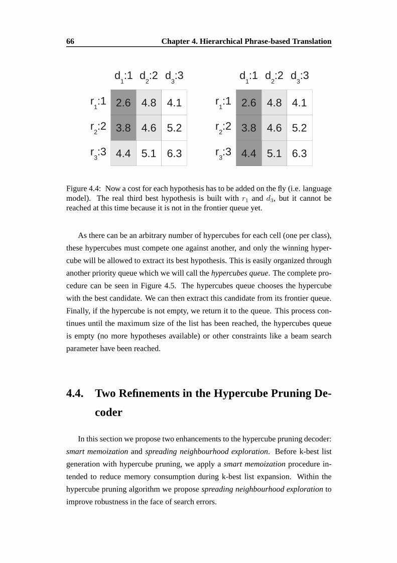
66 Chapter 4. Hierarchical Phrase-based Translation
Figure 4.4: Now a cost for each hypothesis has to be added on the fly (i.e. languagemodel). The real third best hypothesis is built withr1 and d3, but it cannot bereached at this time because it is not in the frontier queue yet.
As there can be an arbitrary number of hypercubes for each cell (one per class),
these hypercubes must compete one against another, and onlythe winning hyper-
cube will be allowed to extract its best hypothesis. This is easily organized through
another priority queue which we will call thehypercubes queue. The complete pro-
cedure can be seen in Figure 4.5. The hypercubes queue chooses the hypercube
with the best candidate. We can then extract this candidate from its frontier queue.
Finally, if the hypercube is not empty, we return it to the queue. This process con-
tinues until the maximum size of the list has been reached, the hypercubes queue
is empty (no more hypotheses available) or other constraints like a beam search
parameter have been reached.
4.4. Two Refinements in the Hypercube Pruning De-
coder
In this section we propose two enhancements to the hypercubepruning decoder:
smart memoizationandspreading neighbourhood exploration. Before k-best list
generation with hypercube pruning, we apply asmart memoizationprocedure in-
tended to reduce memory consumption during k-best list expansion. Within the
hypercube pruning algorithm we proposespreading neighbourhood explorationto
improve robustness in the face of search errors.

4.4. Two Refinements in the Hypercube Pruning Decoder 67
Figure 4.5: Hypothetic situation where 9 hypotheses have been extracted (darkgray squares) and the 10th-best hypothesis goes next. At stage (a), hypercubes areordered in the hypercubes queue by its best reachable hypothesis in the respectivefrontier queues (light gray squares). In this case, hypercube containing hypothesiswith cost 2 is the winner and is extracted. Then, at stage(b), this hypothesis isextracted and two more are added to the frontier queue. Now its best hypothesishas cost 4. Finally, at stage(c) this hypercube is inserted again in the hypercubesqueue, after which the hypercubes queue points to another hypercube with the besthypothesis (cost 3) and the process continues as in stage(a).

68 Chapter 4. Hierarchical Phrase-based Translation
4.4.1. Smart Memoization
One key aspect of the k-best algorithm is its memoization, a dynamic program-
ming technique that consists of calculating partial results once and store for reusing
many times. In this particular case, we calculate once listsof partial translation hy-
potheses associated to each cell of the CYK grid and store forlater use. But, if these
stored lists are big, it also implies strong memory requirements. With smart memo-
ization we alleviate this issue taking advantage of the k-best algorithm itself. After
the parsing stage is completed, it is possible to make a very efficient first sweep
through the backpointers of the CYK grid to count how many times each cell will
be accessed by the k-best generation algorithm. When the k-best list generation is
running, the number of times each cell is visited is logged sothat, as each cell is
visited for the last time, the k-best list associated with each cell is deleted. This
continues until the one k-best list remaining at the top of the chart spans the entire
sentence.
Summing up, smart memoization is a simple garbage collecting procedure that
yields substantial memory reductions for longer sentences. For instance, for the
longest sentence in the tuning set described in Section 4.5 (105 words in length),
smart memoization reduces memory usage during the hypercube pruning stage from
2.1GB to 0.7GB. For average length sentences of approximately 30 words, memory
reductions of 30% are typical.
4.4.2. Spreading Neighbourhood Exploration
When a hypothesis is extracted from a frontier queue, the frontier queue is up-
dated by searching through the neighbourhood of the extracted item in the hyper-
cube to find novel hypotheses to add; if no novel hypotheses are found, that queue
necessarily shrinks. This shrinkage can lead to search errors. Chiang[2007] only
explores the next neighbour through each axis. As shown in Figure 4.6, we require
that new candidates must be added by exploring a neighbourhood which spreads
from the last extracted hypothesis. Each axis of the hypercube is searched (here, to
a depth of 20) until a novel hypothesis is found. In this way, we try to guarantee that
Nnt+1 candidates will always be added to the frontier queue every time a candidate
has been chosen.
Chiang [2007] describes an initialization procedure in which these frontier
queues would be seeded with a single candidate per axis; we initialize each frontier

4.5. A Study of Hiero Search Errors in Phrase-Based Translation 69
Figure 4.6: Spreading neighbourhood exploration within a hypercube, just beforeand after extraction of the item C. Grey squares represent the frontier queue; blacksquares are candidates already extracted. Chiang would only consider adding itemsX to the frontier queue, so the queue would shrink. Spreadingneighbourhood ex-ploration adds candidates S to the frontier queue.
queue to a depth ofbNnt+1, where Nnt is the number of non-terminals in the deriva-
tion andb is a search parameter set throughout to 10. By starting with deep frontier
queues and by forcing them to grow during search we attempt toavoid search errors
by ensuring that the universe of items within the frontier queues does not decrease
as the k-best lists are filled.
4.5. A Study of Hiero Search Errors in Phrase-Based
Translation
We have already hinted in this chapter that the reordering power of a hierarchical
decoder depends solely on the grammar it is using. The grammar is a set of rules
that can be conveniently manipulated. So instead of building standard hierarchical
models we can easily introduce slight modifications, or evenbuild very different
models, with simpler reorderings. This makes it possible tocontrast the hierarchical
decoder with other phrase-based systems.
HIERO MONOTONE HIERO MJ1 HIEROX → 〈V2V1,V1V2〉 X → 〈γ,α〉
X → 〈V ,V 〉 γ, α ∈ (X ∪T)+
X → 〈s,t〉 V → 〈s,t〉s, t ∈ T+ s, t ∈ T+
Table 4.1: Contrast of grammars.T is the set of terminals.

70 Chapter 4. Hierarchical Phrase-based Translation
In particular, in this section we compare the hypercube pruning decoder to
the TTM [Kumaret al., 2006], a phrase-based SMT system implemented with
Weighted Finite-State Transducers[Allauzenet al., 2007]. The system implements
either a monotone phrase order translation, or an MJ1 (maximum phrase jump of
1) reordering model[Kumar and Byrne, 2005]. Relative to the complex move-
ment and translation allowed by Hiero and other models, MJ1 is clearly infe-
rior [Dreyeret al., 2007]; MJ1 was developed with efficiency in mind so as to run
with a minimum of search errors in translation and to be easily and exactly realized
via WFSTs. Even for the large models used in an evaluation task, the TTM system
is reported to run largely without pruning[Blackwoodet al., 2008].
The Hiero decoder can easily be made to implement Monotone phrase-based
or with MJ1 reordering by allowing only a restricted set of rules in addition to the
usual glue rule, as shown in the left-hand column and the middle column, respec-
tively of Table 4.1, where both are contrasted to the standard hierarchical grammar.
Constraining Hiero in this way makes it possible to compare its performance to the
exact WFST TTM implementation and to identify any search errors made by Hiero.
For experiments in Arabic-to-English translation reported in this section
we use all allowed parallel corpora in the NIST MT08 Arabic Constrained
Data track (∼150M words per language). Parallel text is aligned with
MTTK [Deng and Byrne, 2006; Deng and Byrne, 2008]. We use a development set
mt02-05-tuneformed from the odd numbered sentences of the NIST MT02 through
MT05 evaluation sets. Themt02-05-tuneset has 2,075 sentences. Features ex-
tracted from the alignments and used in translation are in common use: target lan-
guage model, source-to-target and target-to-source phrase translation models, word
and rule penalties, number of usages of the glue rule, source-to-target and target-to-
source lexical models, and three rule count features inspired by Bender et al.[2007].
MET [Och, 2003] iterative parameter estimation under IBM BLEU is performedon
the development set. The English language used model is a 4-gram estimated over
the parallel text and a 965 million word subset of monolingual data from the English
Gigaword Third Edition. BLEU score is obtained withmteval-v11b3.
Table 4.2 shows the lowercased IBM BLEU scores obtained by the systems for
mt02-05-tunewith monotone and reordered search, and with MET-optimizedpa-
rameters for MJ1 reordering. For Hiero, an N-best list depthof 10,000 is used
throughout. In the monotone case, all phrase-based systemsperform similarly al-
3See ftp://jaguar.ncsl.nist.gov/mt/resources/mteval-v11b.pl.

4.6. Related Work 71
though Hiero does make search errors. For simple MJ1 reordering, the basic Hiero
search procedure makes many search errors and these lead to degradations in BLEU.
Spreading neighbourhood expansion reduces the search errors and improves BLEU
score significantly but search errors remain a problem. Search errors are even more
apparent after MET. This is not surprising, given thatmt02-05-tuneis the set over
which MET is run: MET drives up the likelihood of good hypotheses at the expense
of poor hypotheses, but search errors often increase due to the expanded dynamic
range of the hypothesis scores.
Monotone MJ1 MJ1+METBLEU SE BLEU SE BLEU SE
a 44.7 - 47.2 - 49.1 -b 44.5 342 46.7 555 48.4 822c 44.7 77 47.1 191 48.9 360
Table 4.2: Phrase-based TTM and Hiero performance onmt02-05-tunefor TTM(a), Hiero (b), Hiero with spreading neighbourhood exploration (c). SE is the num-ber of Hiero hypotheses with search errors.
To sum up, our contrastive experiments prove that spreadingneighbourhood
exploration is a simple yet useful technique to reduce search errors. Nevertheless,
the hypercube pruning decoder is able to perform far more complex reorderings, so
it is expected that search errors may be an issue, particularly as the search space
grows to include the complex long-range movement allowed bythe hierarchical
rules. Importantly, these findings suggest too that a more compact representation
than the k-best lists would improve the hierarchical as lesspruning in searchwould
be required (see discussion in Section 5.3) and thus search errors would be reduced.
4.6. Related Work
Hiero translation systems incorporate many of the strengths of phrase-based
translation systems, such as feature-based translation and strong target language
models, while also allowing flexible translation and movement based on hierarchi-
cal rules extracted from aligned parallel text. In order to put our work into context,
in this section we classify and examine contributions, mainly the ones related to
hierarchical phrase-based translation.

72 Chapter 4. Hierarchical Phrase-based Translation
4.6.1. Hiero Key Papers
Chiang [2005] introduces hierarchical decoding and presents results in
Mandarin-to-English translation. Chiang[2007] explains hierarchical decoding
with three different strategies: the -LM decoder, the Intersection decoder and the
hypercube pruning decoder. The Intersection decoder applies decoding in one sin-
gle pass using the synchronous context-free grammar, whereas the other two divide
the problem in two steps. The first step parses the source sentence and the sec-
ond step retrieves the target translation hypotheses. While the -LM decoder prunes
in search without a language model, the hypercube pruning decoder includes the
language models costs thus applying a more effective pruning strategy that yields
results comparable to the Intersection decoder in faster times. Results are provided
for Chinese-to-English. This paper is probably the most extensive one publicly
available for the research community.
4.6.2. Extensions and Refinements to Hiero
Huang and Chiang[2007] offer several refinements to hypercube pruning to
improve translation speed, i.e. they use a heuristic that attempts to reduce the k-best
within each node. In this work, their enhanced hypercube pruning system is used
for a Pharaoh-like decoder ([Koehn, 2004]) and a tree-to-string (syntax-directed)
decoder.
Li and Khudanpur[2008] report significant improvements in translation speed
by taking unseen n-grams into account within hypercube pruning to minimize lan-
guage model requests. They also propose to use distributed language model servers,
suggesting that the same strategy could be used with the synchronous grammar.
Dyer et al. [2008] extend the translation of source sentences to translation of
input lattices following the algorithm described by Chappelier et al. [1999] that
inserts alternative source words into higher cells of the CYK grid.
The Syntax-Augmented Machine Translation system[Zollmannet al., 2006] in-
corporates target language syntactic constituents in addition to the synchronous
grammars used in translation. Thus, the SAMT system allows many non-terminals
for more meaningful syntactic information. Interestingly, the system uses different
kind of prunings, even during parsing, and uses a ‘Lazier than lazy k-best’ strategy
instead of hypercube pruning.
Venugopal et al.[2007] introduce a Hiero variant with relaxed constraints for
4.6. Related Work 73
hypothesis recombination during parsing; speed and results are comparable to those
of hypercube pruning.
Shen et al.[2008] make use of target dependency trees and a target depen-
dency language model during decoding. Marton and Resnik[2008] exploit shal-
low correspondences of hierarchical rules with source syntactic constituents ex-
tracted from parallel text, an approach also introduced by Chiang [2005] and in-
vestigated by Vilar et al.[2008]. Chiang et al[2008] extend this work training
with coarse-grained and fine-grained features using the Margin Infused Relaxed Al-
gorithm [Crammer and Singer, 2003; Crammeret al., 2006] rather than traditional
MET [Och, 2003]. They also introduce what they define asstructural distortion
features, trying to model the influence of the non-terminal height on reorderings.
As yet another alternative approach, Venugopal et al.[2009] refine probabilistic
synchronous context-free grammars with soft non-terminalsyntactic labels.
In order to tackle constituent-boundary-crossing problems, Setiawan et
al. [2009] design special features based simply on the topological order of func-
tion words. Marton and Resnik also add features for constituent-boundary-
crossing synchronous rules and claim significant improvements[2008]. Zhang and
Gildea[2008] propose a multi-pass variant of a Hiero system as an alternative to
Minimum-Bayes Risk[Kumar and Byrne, 2004]. Finally, Blunsom et al.[2008]
discuss procedures to combine discriminative latent models with hierarchical SMT.
4.6.3. Hierarchical Rule Extraction
Zhang and Gildea[2006] propose binarization for synchronous grammars as a
means to control search complexity arising from more linguistically syntactic hi-
erarchical grammars. Zhang et al.[2008] describe a linear algorithm, a modified
version of shift-reduce, to extract phrase pairs organizedinto a tree from which
hierarchical rules can be directly extracted. Lopez[2007] extracts rules on-the-fly
from the training bitext during decoding, searching efficiently for rule patterns using
suffix arrays[Manber and Myers, 1990]. He et al.[2009] filter the rule extraction
using theC-valuemetric [Frantzi and Ananiadou, 1996], which takes into account
four factors: the length of the phrase, the frequency of thisphrase in the training
corpus, the frequency as a substring in longer phrases and the number of distinct
phrases that contain this phrase as a substring.

74 Chapter 4. Hierarchical Phrase-based Translation
4.6.4. Contrastive Experiments and Other Hiero Contributions
Chiang et al.[2005] contrast hierarchical decoding with phrase-based decoding
using patterns built on part-of-speech of source sequencesto analyze when and why
hierarchical decoding has better word reordering capabilities.
Zollman et al. [2008] compare phrase-based, hierarchical and syntax-
augmented decoders for translation of Arabic, Chinese, andUrdu into English, and
they find that attempts to expedite translation by simple schemes which discard rules
also degrade translation performance.
Lopez [2008] explores whether lexical reordering or the phrase discontiguity
inherent in hierarchical rules explain improvements over phrase-based systems.
Auli et al. [2009] contrast hierarchical and phrase-based models. Their ex-
periments suggest that the differences between both modelsare structurally quite
small and hence hypotheses ranking accounts for most of the differences in per-
formance. Lopez[2009] formulates theoretically the statistical translation problem
as a weighted deduction system that covers phrase-based andhierarchical models.
Although this is an abstract work, it shows that deductive logic could be in the fu-
ture a great practical framework for fair comparisons between both models and their
multiple variants, suggesting that in general it is quite difficult to track down the rea-
sons for which one system performs better than another when the implementation is
completely different. Hoang et al.[2009] extend Moses to build a common frame-
work for hierarchical, syntax-based and phrase-based models in order to facilitate
comparisons between these three models.
4.7. Conclusions
In this chapter we have described hierarchical phrase-based translation. In par-
ticular, we have described models and implementation of thehypercube pruning
decoder, which consists of two steps. The first step is a variant of the CYK parser
on the source side with hypotheses recombination and no pruning. The second step
is the k-best algorithm, which traverses each cell of the CYKgrid. In each cell,
a priority queue of hypercubes (the hypercubes queue) is used to extract the best
candidates. In turn, each hypercube implements the hypercube pruning procedure
by means of another priority queue calledfrontier queue.
We then present two enhancements to the basic decoder.Smart memoizationis

4.7. Conclusions 75
a garbage collecting procedure for more efficient memory usage. Spreading neigh-
bourhood explorationprevents many search errors by not only examining neigh-
bours next to the chosen item in the hypercube, but extendingthis search through
each axis to a fixed depth. We demonstrate this by using two simple phrase-based
systems almost free of search errors as a contrast for the hypercube pruning decoder.
As it is simple to reproduce strictly the search space of these systems with the ap-
propriate grammar, we perform a fair comparison of search errors. To end with this
chapter, we have introduced several papers that are relevant to hierarchical phrase-
based translation — already a successful research strand after only a few years, and
very attractive to MT researchers.
The experimental part and the enhancements to hypercube pruning pre-
sented in this chapter have partially motivated a paper in the EACL confer-
ence[Iglesiaset al., 2009c].
At this point we have two paths to follow. The first path is related to the fact that
a hierarchical decoder is as powerful as the grammar it is relying on. To modify the
grammar is trivial. Such a thing endows this framework with aflexibility we expect
to exploit with more informed strategies as a post-processing step to the initial rule
extraction described in Section 4.2. In this sense, up to nowwe have only scratched
the surface with the experimental part of this chapter. In Chapter 5 we will work
with several variations of a standard hierarchical grammar, attempting to design
more efficient search spaces.
The second path leads to a lattice implementation of a hierarchical decoder,
attempting to reduce search errors found for the hypercube pruning decoder even
for trivial models such as monotone phrase-based and MJ1. Wewill deal with this
in Chapter 6.


Chapter 5Hierarchical Grammars
Contents5.1. Introduction . . . . . . . . . . . . . . . . . . . . . . . . . . . 77
5.2. Experimental Framework . . . . . . . . . . . . . . . . . . . . 78
5.3. Preliminary Discussions . . . . . . . . . . . . . . . . . . . . . 79
5.4. Filtering Strategies for Practical Grammars . . . . . . . . . 83
5.5. Large Language Models and Evaluation . . . . . . . . . . . . 99
5.6. Shallow-N grammars and Extensions . . . . . . . . . . . . . 100
5.7. Conclusions . . . . . . . . . . . . . . . . . . . . . . . . . . . . 105
5.1. Introduction
We now face the problem of how to design the hierarchical search space we ac-
tually want to explore with both our hypercube pruning decoder andHiFST, to be
introduced in the next chapter. A hierarchical search spaceis defined by the sen-
tence we wish to translate and a synchronous context-free grammar, which basically
is a very big set of rules we have learnt from the training corpus. As imposing re-
strictions to the sentences we translate is completely out of the point, the only way
of attempting to model our search space in this context is to modify the grammar.
After describing in Section 5.2 the experimental framework, we discuss in Sec-
tion 5.3 a few key concepts we have to keep in mind as search space designers.
Several techniques will be described in order to analyze andreduce this grammar
in Section 5.4. We do this based on the structural propertiesof rules and develop

78 Chapter 5. Hierarchical Grammars
strategies to identify and remove redundant or harmful rules. We identify groupings
of rules based on non-terminals and their patterns and assess the impact on transla-
tion quality and computational requirements for each givenrule group. We find that
with appropriate filtering strategies rule sets can be greatly reduced in size without
impact on translation performance. We also describe a ‘shallow’ search through
hierarchical rules which greatly speeds translation without any effect on quality for
the Arabic-to-English translation task. We show rescoringexperiments for our best
configuration on Section 5.5. Finally we propose new grammars in Section 5.6. In
particular, in Section 5.6.1 we will extend this shallow configuration into a new type
of hierarchical grammars: theshallow-N grammars.
5.2. Experimental Framework
For translation experiments reported along this chapter inArabic-to-
English, alignments are generated with MTTK[Deng and Byrne, 2006;
Deng and Byrne, 2008] over all allowed parallel corpora in the NIST MT08
Arabic Constrained Data track(∼150M words per language). We use a develop-
ment setmt02-05-tuneformed from the odd numbered sentences of the NIST MT02
through MT05 evaluation sets; the even numbered sentences form the validation set
mt02-05-test. Themt02-05-tuneset has 2,075 sentences. For a comparative with
other translation systems, we use the NIST MT08 Arabic-to-English translation
task. Features extracted from the alignments and used in translation are in common
use: target language model, source-to-target and target-to-source phrase translation
models, word and rule penalties, number of usages of the gluerule, source-to-target
and target-to-source lexical models, and three rule count features inspired by
Bender et al.[2007]. MET [Och, 2003] iterative parameter estimation under IBM
BLEU is performed on the development set. The English language used model
is a 4-gram estimated over the parallel text and a 965 millionword subset of
monolingual data from the English Gigaword Third Edition. All the experiments
are performed with our hypercube pruning decoder (HCP) explained in Chapter 4.
BLEU score is obtained withmteval-v11b1. Experiments with other language pairs
will be shown in the next chapter.
1See ftp://jaguar.ncsl.nist.gov/mt/resources/mteval-v11b.pl.

5.3. Preliminary Discussions 79
5.3. Preliminary Discussions
5.3.1. Completeness of the Model
Figure 5.1: Model versus reality.
Researchers build models to imitate reality. But the contrast between model and
reality, depicted in Figure 5.1, is something that researchers should always keep in
mind, because we are (or should be) attempting to bridge the gap between both of
them. IfR is the reality andM is the model,R ∩M corresponds to the reality we
have successfully mimicked, whereasR − R ∩ M corresponds to that part of the
reality the model is not capable of generating. This is anundergenerationproblem.
Conversely,M−R∩M refers to the part of the model that does not correspond to the
reality. We call itovergeneration. Both terms have been used regularly in the Pars-
ing literature. It is not very common to find these terms in theStatistical Machine
Translation literature2. Interestingly, for instance papers from the rule-based system
developed for the Eurotra Project in the 80s used this term[Varile and Lau, 1988].
We advocate for the use of these terms as now many state-of-the-art MT sys-
tems embed parsers in the pipeline decoding process, so it would only seem natural
to keep coherence. As an example, in Figure 5.2 overgeneration occurs because
different derivations based on the same rules give rise to different translations. This
process is not necessarily a bad thing in that it allows new translations to be synthe-
sized from rules extracted from training data; a strong target language model, such
as a high order n-gram, is typically relied upon to discard unsuitable hypotheses.
2A very recent example is a paper proposed by Setiawan et al.[2009].The “Stochastic InversionTransducer Grammar" paper[Wu, 1997] does not use this term, but the author is clearly concernedabout the issue.

80 Chapter 5. Hierarchical Grammars
R1: X→〈s1 X ,A X〉R2: X→〈X s3,X C〉R3: X→〈s2,B〉
Figure 5.2: Example of multiple translation sequences froma simple grammar frag-ment showing variability in reordering in translation of the source sequences1s2s3.
However overgeneration does complicate translation in that many hypotheses are
introduced only to be subsequently discarded.
For instance, thinking in terms of overgeneration and undergeneration, com-
mon sense dictates that similar languages (such as Spanish-English) would probably
need smaller and simpler models than differently structured languages pairs (such
as Chinese-English) that require very long reorderings. Soif we use a Chinese-
to-English model as a Spanish-to-English model we will probably suffer of se-
vere overgeneration. And conversely, applying the Spanish-to-English model to
a Chinese-to-English task would probably lead to undergeneration problems.
So this suggests that perhaps we should build different models for different
translation tasks. Precisely one of the advantages of usinga parsing algorithm such
as CYK is that it relies on a grammar that could be easily manipulated. We have
already seen a good example of this flexibility in Chapter 4, in which two simple
grammars were built, corresponding to a monotone phrase-based model and an ex-
tended version that includes a trivial reordering scheme defined with a few extra
rules.
Researchers usually take their models to the limits. When this happens, usually
the search space gets too big for the hardware it is running on. In turn, this forces
to discard hypotheses in order to make the decoding process tractable. We use the
term pruning for this hypotheses discarding process. Depending on the decoder,
two kind of pruning procedures may be needed:
Final Prune. Once we have built a translation search space, it will probably
be far too big to handle, so this requires a pruning stage, which will be con-

5.3. Preliminary Discussions 81
cordant with the model itself (but not necessarily with reality). So we expect
that if the model is good enough the probability of undergenerating will be
small.
Search Pruneor Pruning in Search. The translation search space is so big
that we have to prune whilst we are building it. Pruning partial search spaces
is dangerous as it leads quite inevitably tosearch errors, i.e. to discard hy-
potheses that would turn out to be winning candidates. Not only do search
errors affect the best hypothesis. Typically we work with k-best hypotheses
or lattices — to incur in search errors is to degrade the quality of all these best
hypotheses the k-best list or lattice is encompassing.
For our purposes we will extend the concept of undergeneration to the final
translation proposed by any SMT decoder. In other words, if the decoder is not able
to generate the correct translation hypothesis, this couldbe due to two reasons. The
first one is simply the grammar: it lacks the power to generatethat hypothesis. This
is a problem of design in the sense that the grammar is completely definedbefore
the decoding stage. Hence, it should be relatively easy to define strategies to correct
this problem. However, by means of pruning in search the decoding procedure itself
may incur insearch errors. If due to these search errors good translation hypotheses
are discarded we have a spurious kind of undergeneration problem, very difficult to
control. No matter how powerful a decoder is, if forced to apply pruning in search
consequently there will be search errors producing undergeneration problems.
Related to overgeneration and undergeneration, another limitation we have to
face is thespurious ambiguity, another concept inherited from parsing, and already
discussed by Chiang[2007]. This phenomenon occurs when different derivations
lead to the same translation hypotheses. This is due in part to thehypercube prun-
ing procedure, which enumerates all distinct hypotheses to a fixed depth by means
of k-best hypotheses lists. If enumeration was not necessary, or if the lists could
be arbitrarily deep, there might still be many duplicate derivations but at least the
hypothesis space would not be impoverished. This problem may be partially alle-
viated by means of a hypotheses recombination strategy. Thebigger the size of the
list (or the lattice), the better. But indeed this is a costlyprocedure. In practice, due
to hardware restrictions it is not possible to avoid a weightmass loss, as we only
keep the best weight for the recombined hypotheses.
Concluding, as search space designers we would like to find grammars that build

82 Chapter 5. Hierarchical Grammars
tractable translation search spaces, of course containinggood translation hypothe-
ses, but as small as possible in order to avoid the spurious ambiguity and spurious
undergeneration produced by search errors. Of course, no sensible researcher will
lose 1 point BLEU just to avoid search errors — but at least conceptually, smaller
search spaces with no search errors seem a safer standing point for further improve-
ments. We feel that keeping this always in mind is a healthy exercise.
5.3.2. Do We Actually Need the Complete Grammar?
Large-scale hierarchical SMT involves automatic rule extraction from aligned
parallel text, model parameter estimation, and the use of hypercube pruning k-
best list generation in hierarchical translation. The number of hierarchical rules
extracted according to the procedure explained in Section 4.2 far exceeds the num-
ber of phrase translations typically found in aligned text.While this may lead to
improved translation quality, there is also the risk of lengthened translation times
and increased memory usage, along with possible search errors (as discussed be-
fore) due to the pruning procedures needed in search.
Interestingly, for instance Auli et al.[2009] suggest that limiting the number of
translations for the same source phrase does affect performance. But in fact, we feel
it is possible that discarding certain rules from this grammar is not harmful at all,
but even helps to improve the performance. It should be notedthat due to the nature
of the (hierarchical) phrase extraction, it is likely that the complete grammar should
overgenerate because it is not imposed as a restriction thatthe rules are actually
used in even one complete derivation of any sentence throughout the training set.
Thus perhaps an important number of these rules are actuallynoisy, lead to spurious
ambiguity and even harm the MET optimization procedure.
During rule extraction we obtain from alignments only thoserules that are rele-
vant to our given test set; for computation of backward translation probabilities we
log general counts of target-side rules but discard unneeded rules. Even with this
restriction, our initial grammar formt02-05-tuneexceeds 175M rules, of which only
0.62M are simple phrase pairs.
The question is whether all these rules are needed for translation. If the grammar
can be reduced without reducing translation quality, both memory efficiency and
translation speed can be increased. Previously published approaches to reducing
the grammar include: enforcing a minimum span of two words per non-terminal

5.4. Filtering Strategies for Practical Grammars 83
[Lopez, 2008], which would reduce our set to 115M rules; or a minimum count
(mincount) threshold[Zollmannet al., 2008], which would reduce our set to 78M
(mincount=2) or 57M (mincount=3) rules. Shen et al.[2008] describe the result of
filtering rules by insisting that target-side rules are well-formed dependency trees.
This reduces their grammar from 140M to 26M rules. This filtering leads to a
degradation in translation performance (see Table 2 of Shenet al. [2008]), which
they counter by adding a dependency LM in translation. As another reference point,
Chiang[2007] reports Chinese-to-English translation experiments based on 5.5M
rules.
Zollmann et al.[2008] report that filtering rules en masse leads to degradation
in translation performance. Rather than apply a coarse filtering, such as a mincount
for all rules, we now propose a more syntactic approach and further classify our
rules according to theirpatternand apply different filters to each pattern depending
on its value in translation. The premise is that some patterns are more important
than others.
5.4. Filtering Strategies for Practical Grammars
In this section we propose the following four filtering strategies in order to re-
duce the complete grammar:
1. Filtering by rule pattern.
2. Filtering by rule count.
3. Filtering by selective mincounts applied to groups of patterns (classes).
4. Filtering by rewriting hierarchical grammars as shallowgrammars.
The following subsections will study each type of filtering.
5.4.1. Rule Patterns
Hierarchical rulesX → 〈γ,α〉 are composed of non-terminals and subsequences
of terminals, any of which we callelements. In the source, a maximum of two
non-adjacent non-terminals is allowed, as explained in Section 4.2. Leaving aside
rules without non-terminals (i.e. phrase pairs as used in phrase-based translation),
rules can be classed by their number of non-terminals, Nnt, and their number of

84 Chapter 5. Hierarchical Grammars
elements, Ne. There are5 possible classes associated to hierarchical rules: Nnt.Ne=
1.2, 1.3, 2.3, 2.4, 2.5. The phrase-based pattern is associated to Nnt.Ne= 0.1.
Class Rule PatternNnt.Ne 〈source, target〉 Types % NSP
〈wX1 , wX1〉 1185028 0.68 51879〈wX1 , wX1w〉 153130 0.09 25525
1.2 〈wX1 , X1w〉 97889 0.06 16090〈X1w , wX1〉 72633 0.04 14710〈X1w , wX1w〉 106603 0.06 22470〈X1w , X1w〉 1147576 0.66 52659
〈wX1w , wX1〉 989540 0.57 5815761.3 〈wX1w , wX1w〉 32903522 18.79 12730783
〈wX1w , X1w〉 951116 0.54 597710〈X1wX2 , wX1wX2〉 178325 0.10 21307〈X1wX2 , wX1wX2〉 4840 0.00 3042〈X1wX2 , wX1wX2〉 64293 0.04 15236〈X1wX2 , wX1X2w〉 6644 0.00 3840〈X1wX2 , X1wX2〉 1554656 0.89 46429〈X1wX2 , X1wX2w〉 243280 0.14 25142〈X1wX2 , X1X2w〉 69556 0.04 15293
2.3 〈X2wX1 , wX1wX2〉 41529 0.02 8760〈X2wX1 , wX1wX2w〉 5706 0.00 2469〈X2wX1 , wX1X2〉 35641 0.02 11249〈X2wX1 , wX1X2w〉 9297 0.01 4536〈X2wX1 , X1wX2〉 39163 0.02 9886〈X2wX1 , X1wX2w〉 28571 0.02 7481〈X2wX1 , X1X2w〉 33230 0.02 9844
Table 5.1: Hierarchical rule patterns (〈source,target〉) classed by number of non-terminals (Nnt) and number of elements (Ne). Additionally, types (distinct rules),percentage (%) and NSP (number of source phrases per rule pattern) are shown foreach pattern in the grammar extracted formt02-05-tune.
Given any rule, it is easy to replace every sequence of terminals by a single
symbol ‘w’. This is useful to classify rules, as any rule belongs to only one pattern,
whereas patterns encompass many rules. Some examples of extracted rules and
their corresponding pattern follow, where Arabic is shown in Buckwalter encoding.

5.4. Filtering Strategies for Practical Grammars 85
Class Rule PatternNnt.Ne 〈source, target〉 Types % NSP
〈wX1wX2 , wX1wX2〉 26901823 15.36 8711914〈wX1wX2 , wX1wX2w〉 2534510 1.45 1427240〈wX1wX2 , wX1X2〉 744328 0.43 433902〈wX1wX2 , wX1X2w〉 1624092 0.93 1057591〈wX1wX2 , X1wX2〉 850860 0.49 470340〈wX1wX2 , X1wX2w〉 159895 0.09 121615〈wX1wX2 , X1X2w〉 10719 0.01 9808〈wX2wX1 , wX1wX2〉 349176 0.20 209982〈wX2wX1 , wX1wX2w〉 68333 0.04 51854〈wX2wX1 , wX1X2〉 172797 0.10 113305〈wX2wX1 , wX1X2w〉 131517 0.08 93973〈wX2wX1 , X1wX2〉 36144 0.02 28630〈wX2wX1 , X1wX2w〉 70063 0.04 56831
2.4 〈wX2wX1 , X1X2w〉 8172 0.00 7566〈X1wX2w , wX1wX2〉 79888 0.05 66482〈X1wX2w , wX1wX2w〉 1136689 0.65 674745〈X1wX2w , wX1X2〉 3709 0.00 3518〈X1wX2w , wX1X2〉 1984021 1.13 1257279〈X1wX2w , X1wX2〉 841467 0.48 451561〈X1wX2w , X1wX2w〉 26053969 14.88 853373〈X1wX2w , X1X2w〉 487070 0.28 320415〈X2wX1w , wX1wX2〉 97710 0.06 73306〈X2wX1w , wX1wX2w〉 106627 0.06 65005〈X2wX1w , X1X2〉 13774 0.01 12262〈X2wX1w , wX1X2w〉 180870 0.10 125180〈X2wX1w , X1wX2〉 27911 0.02 24044〈X2wX1w , X1wX2w〉 259459 0.15 178288〈X2wX1w , X1X2w〉 115242 0.07 80870
Table 5.2: Hierarchical rule patterns (continued) classedby number of non-terminals (Nnt) and number of elements (Ne). Additionally, types, percentage (%)and NSP (number of source phrases per rule pattern) are shownfor each pattern inthe grammar extracted formt02-05-tune.

86 Chapter 5. Hierarchical Grammars
Class Rule PatternNnt.Ne 〈source, target〉 Types % NSP
〈wX1wX2w , wX1wX2〉 2151252 1.23 1590126〈wX1wX2w , wX1wX2w〉 61704299 35.24 32926332〈wX1wX2w , wX1X2〉 4025 0.00 3896〈wX1wX2w , wX1X2w〉 3149516 1.80 2406883〈wX1wX2w , X1wX2〉 87944 0.05 81088〈wX1wX2w , X1wX2w〉 2330797 1.33 1679725
2.5 〈wX1wX2w , X1X2w〉 9313 0.01 8675〈wX2wX1w , wX1wX2〉 114852 0.07 98956〈wX2wX1w , wX1wX2w〉 275810 0.16 212655〈wX2wX1w , wX1X2〉 7865 0.00 7507〈wX2wX1w , wX1X2w〉 205801 0.12 161170〈wX2wX1w , X1wX2〉 6195 0.00 5956〈wX2wX1w , X1wX2w〉 90713 0.05 80661〈wX2wX1w , X1X2w〉 6149 0.00 5886
Table 5.3: Hierarchical rule patterns (continued) classedby number of non-terminals (Nnt) and number of elements (Ne). Additionally, types, percentage (%)and NSP (number of source phrases per rule pattern) are shownfor each pattern inthe grammar extracted formt02-05-tune.
Pattern〈wX1 , wX1w〉 :
〈w+ qAl X1 , theX1 said〉
Pattern〈wX1w , wX1〉 :
〈fy X1 kAnwn Al>wl , on decemberX1〉
Pattern〈wX1wX2 , wX1wX2w〉 :
〈Hl X1 lAzmp X2 , aX1 solution to theX2 crisis〉
By ignoring the identity and the number of adjacent terminals, the rule pattern
represents a natural generalization of any synchronous rule, capturing its structure
and the type of reordering it encodes. Intuitively, we rely on patterns because we
are expecting them to be capturing some amount of syntactic information that could
help, for instance to guide a filtering procedure. Tables 5.1, 5.2 and 5.3 present all
the patterns extracted for the development setmt02-05-tuneand grouped into their
respective classes Nnt.Ne= 1.2, 1.3, 2.3, 2.4, 2.5 (left column). In total, including
the phrase-based pattern (〈w, w〉 or Nnt.Ne= 0.1) there are 66 possible rule patterns.
The three columns to the right show the number of distinct rules (types) found in the
development set, the percentage of types relative to the whole grammar (%) and the
number of source phrases per rule pattern, this is, how many hierarchical phrases

5.4. Filtering Strategies for Practical Grammars 87
does each pattern actually translate.
The table shows that some patterns have many more types than others. Pat-
terns with two non-terminals (Nnt=2) include many more types than patterns with
Nnt=1. Additionally, patterns with two non-terminals that also have a monotonic
relationship between source and target non-terminals are much more diverse than
their reordered counterparts. This is particularly notorious for identical patterns
(rule patterns with source pattern identical to target pattern). For instance, rule pat-
tern 〈wX1wX2w,wX1wX2w〉 contains by itself more than the third of all the rule
types (Table 5.3), whereas its reordered counterpart〈wX1wX2w,wX2wX1w〉 only
represents less than0.2%.
To clarify things, we formalize the previous ideas.
A rule pattern— or simply pattern — is a generalization of any rule by
rewriting in the right-hand side of the rule sequences of adjacent terminals
as one single letter. By convention this letter will bew (indicating word, i.e.
terminal string,w ∈ T+). Non-terminals are left untouched.
A source pattern is the part of the rule pattern corresponding to the source of
the synchronous rule. Similarly, a target pattern corresponds to the target of
the synchronous rule.
Rule patterns are calledhierarchical if they correspond to hierarchical rules.
There is only one pattern corresponding to all the phrase-based rules, and thus
we call it thephrase-based pattern.
A rule pattern is tagged asidenticalif the source pattern and the target pattern
are identical. For instance,〈wX1,wX1〉 is an identical rule pattern.
A rule pattern is tagged asmonotonic— or monotone— if the non-terminals
of the source and the target patterns have identical ordering. If not, this pattern
is called reordered. For instance, 〈wX1wX2w,wX1wX2w〉 is a monotone
pattern, whereas〈wX1wX2w,wX2wX1〉 is a reordered pattern.
5.4.2. Quantifying Pattern Contribution
In order to quantify the contribution of each pattern, we propose the following
experiment. We define grammars that combine the phrase-based rules with hierar-
chical rules belonging to a single pattern. Using a phrase-based configuration as the

88 Chapter 5. Hierarchical Grammars
baseline reference, it is easy to measure the contribution of each pattern alone by
comparing performance.
The results are shown in Tables 5.4, 5.5 and 5.6. These experiments have been
performed with no MET optimization and small k-best lists (i.e. k=100). In order
to speed up the translation system, these experiments are performed using shallow
grammars, its usage to be explained and justified in Section 5.4.4. The contribu-
tion of all these single patterns to phrase-based rules are measured as a difference
of BLEU scores, (seediff column). Class Nnt.Ne=0.1 represents the baseline score
with only phrase-based rules. The best contribution is provided by adding 64293
rules belonging to pattern〈X1wX2,wX1wX2〉, with an increase in performance
of 2.5 BLEU (see Table 5.4). It is followed closely by two patterns belonging
to class Nnt.Ne=1.2: 〈X1w,wX1〉 (adding +2.3 BLEU) and〈wX1,X1w〉 (adding
+2.2 BLEU). These patterns encompass 72633 and 97889 types respectively. On
the other hand, pattern〈X1wX2,X1wX2〉, encompassing more than 1.5 million
types, is not able to improve performance — actually the performance decreased
in −0.1 BLEU. Interestingly, we also find that many other rule patterns show no
improvements at all, for instance patterns〈X1w,X1w〉, 〈X2wX1,wX1wX2w〉 and
〈wX1,wX1〉.
All these results suggest that the importance of a rule pattern has nothing to do
with the number of rules it encompasses. Of course, a question that could arise is
whether these experiments act as an oracle for grammars combining different rule
patterns, as it could be possible that this combination of patterns would somehow
produce certain synergy that a single pattern is not able to reflect. To answer this
question, let us consider what would happen if we now take a new baseline consist-
ing of both the previous phrase-based grammar and rules belonging to the pattern
〈X1wX2,wX1wX2〉, which yielded the best improvement. We repeat the previous
experiment for a few selected patterns among those with the best contribution to
performance. Table 5.7 shows that the relative improvementof each pattern to the
new baseline, depicted in columndiff, is lower than the isolated contribution to the
pure monotone phrase-based grammar, probably due to spurious ambiguity.
In conclusion, these experiments suggest that the contribution of isolated rule
patterns to the phrase-based grammar are optimistic oracles of their overall im-
provement in a complex grammar, and perhaps this knowledge could be used to
build a practical grammar.

5.4. Filtering Strategies for Practical Grammars 89
Class Rule PatternNnt.Ne 〈source, target〉 Types BLEU diff
0.1 〈w , w〉 615190 44.3 -+ 〈wX1 , wX1〉 1185028 44.3 0+ 〈wX1 , wX1w〉 153130 46.1 +1.8
1.2 + 〈wX1 , X1w〉 97889 46.5 +2.2+ 〈X1w , wX1〉 72633 46.6 +2.3+ 〈X1w , wX1w〉 106603 45.5 +1.2+ 〈X1w , X1w〉 1147576 43.3 0
+ 〈wX1w , wX1〉 989540 45.1 +0.81.3 + 〈wX1w , wX1w〉 32903522 44.7 +0.3
+ 〈wX1w , X1w〉 951116 45.6 +1.3+ 〈X1wX2 , wX1wX2〉 178325 45.2 +0.9+ 〈X1wX2 , wX1wX2〉 4840 44.4 +0.1+ 〈X1wX2 , wX1wX2〉 64293 46.8 +2.5+ 〈X1wX2 , wX1X2w〉 6644 44.4 +0.1+ 〈X1wX2 , X1wX2〉 1554656 44.2 -0.1+ 〈X1wX2 , X1wX2w〉 243280 46.2 +1.9+ 〈X1wX2 , X1X2w〉 69556 44.4 +0.1
2.3 + 〈X2wX1 , wX1wX2〉 41529 44.4 +0.1+ 〈X2wX1 , wX1wX2w〉 5706 44.3 0+ 〈X2wX1 , wX1X2〉 35641 44.6 +0.3+ 〈X2wX1 , wX1X2w〉 9297 44.3 0+ 〈X2wX1 , X1wX2〉 39163 44.8 +0.5+ 〈X2wX1 , X1wX2w〉 28571 44.3 0+ 〈X2wX1 , X1X2w〉 33230 44.5 +0.2
Table 5.4: Scores for grammars using one single hierarchical pattern onmt02-05-tuneset (k=100). The right column (diff ) shows the improvement relative to thebaseline phrase-based grammar (Nnt.Ne=0.1).

90 Chapter 5. Hierarchical Grammars
Class Rule PatternNnt.Ne 〈source, target〉 Types BLEU diff
+ 〈wX1wX2 , wX1wX2〉 26901823 45.0 +0.7+ 〈wX1wX2 , wX1wX2w〉 2534510 44.7 +0.4+ 〈wX1wX2 , wX1X2〉 744328 45.0 +0.7+ 〈wX1wX2 , wX1X2w〉 1624092 44.6 +0.3+ 〈wX1wX2 , X1wX2〉 850860 45.3 +1.0+ 〈wX1wX2 , X1wX2w〉 159895 44.4 +0.1+ 〈wX1wX2 , X1X2w〉 10719 44.4 +0.1+ 〈wX2wX1 , wX1wX2〉 349176 44.6 +0.3+ 〈wX2wX1 , wX1wX2w〉 68333 44.4 +0.1+ 〈wX2wX1 , wX1X2〉 172797 44.4 +0.1+ 〈wX2wX1 , wX1X2w〉 131517 44.5 +0.2+ 〈wX2wX1 , X1wX2〉 36144 44.4 +0.1+ 〈wX2wX1 , X1wX2w〉 70063 44.4 +0.1
2.4 + 〈wX2wX1 , X1X2w〉 8172 44.4 +0.1+ 〈X1wX2w , wX1wX2〉 79888 44.4 +0.1+ 〈X1wX2w , wX1wX2w〉 1136689 44.5 +0.2+ 〈X1wX2w , wX1X2〉 3709 44.3 0+ 〈X1wX2w , wX1X2〉 1984021 44.7 +0.4+ 〈X1wX2w , X1wX2〉 841467 45.0 +0.7+ 〈X1wX2w , X1wX2w〉 26053969 45.0 +0.7+ 〈X1wX2w , X1X2w〉 487070 45.4 +1.1+ 〈X2wX1w , wX1wX2〉 97710 44.5 +0.2+ 〈X2wX1w , wX1wX2w〉 106627 44.4 +0.1+ 〈X2wX1w , X1X2〉 13774 44.4 +0.1+ 〈X2wX1w , wX1X2w〉 180870 44.4 +0.1+ 〈X2wX1w , X1wX2〉 27911 44.4 +0.1+ 〈X2wX1w , X1wX2w〉 259459 44.7 +0.4+ 〈X2wX1w , X1X2w〉 115242 44.4 +0.1
Table 5.5: Scores for grammars using one single hierarchical pattern onmt02-05-tuneset (k=100)(continued). The right column (diff ) shows the improvement rela-tive to the baseline phrase-based grammar(Nnt.Ne=0.1), in Table 5.4.

5.4. Filtering Strategies for Practical Grammars 91
Class Rule PatternNnt.Ne 〈source, target〉 Types BLEU diff
+ 〈wX1wX2w , wX1wX2〉 2151252 44.4 +0.1+ 〈wX1wX2w , wX1wX2w〉 61704299 44.5 +0.2+ 〈wX1wX2w , wX1X2〉 4025 44.3 0+ 〈wX1wX2w , wX1X2w〉 3149516 44.5 +0.2+ 〈wX1wX2w , X1wX2〉 87944 44.4 +0.1+ 〈wX1wX2w , X1wX2w〉 2330797 44.6 +0.3
2.5 + 〈wX1wX2w , X1X2w〉 9313 44.4 +0.1+ 〈wX2wX1w , wX1wX2〉 114852 44.4 +0.1+ 〈wX2wX1w , wX1wX2w〉 275810 44.4 +0.1+ 〈wX2wX1w , wX1X2〉 7865 44.3 0+ 〈wX2wX1w , wX1X2w〉 205801 44.4 +0.1+ 〈wX2wX1w , X1wX2〉 6195 44.3 0+ 〈wX2wX1w , X1wX2w〉 90713 44.4 +0.1+ 〈wX2wX1w , X1X2w〉 6149 44.3 0
Table 5.6: Scores for grammars using one single hierarchical pattern onmt02-05-tuneset (k=100)(continued). The right column (diff ) shows the improvement rela-tive to the baseline phrase-based grammar(Nnt.Ne=0.1), in Table 5.4.
Class Rule PatternNnt.Ne 〈source, target〉 Types BLEU diff
〈w,w〉 + 〈X1wX2 , wX1wX2〉 679483 46.8 -+ 〈wX1 , wX1w〉 153130 47.4 +0.6
1.2 + 〈wX1 , X1w〉 97889 47.3 +0.5+ 〈X1w , wX1〉 72633 46.9 +0.1
1.3 + 〈wX1w , wX1〉 951116 46.9 +0.12.3 + 〈X1wX2 , X1wX2w〉 243280 47.4 +0.62.4 + 〈wX1wX2 , X1wX2〉 850860 47.2 +0.42.5 + 〈wX1wX2w , X1wX2w〉 2330797 46.8 0
Table 5.7: Scores for grammars adding a single rule pattern to the new baselinewhich consists of phrase-based and〈X1wX2,wX1X2〉 rules. The right column(diff ) shows the improvement relative to the baseline grammar, now a combina-tion of phrase-based rules and a single hierarchical pattern ( 〈w,w〉 + 〈X1wX2,wX1wX2〉).

92 Chapter 5. Hierarchical Grammars
5.4.3. Building a Usable Grammar
Grammar Configuration rules BLEUG01 Phrase-based 0.62 44.7G02 G01 + Nnt.Ne=1.2 3.2 47.5G03 G02 + Nnt.Ne=1.3, mincount=5 5.8 47.8G04 G02 + Nnt.Ne=1.3 mincount= 10 4.4 47.7G05 G03 + Nnt.Ne=2.3 mincount=5 7.4 47.8G06 G05 - 2nt monotone rules 5.8 47.9G07 G06 + Nnt.Ne=2.5, mincount=5 8.6 47.9G08 G06 + Nnt.Ne=2.5, mincount=10 6.9 47.9G09 G07 - 2nt monotone rules 5.8 48.0G10 G08 - 2nt monotone rules 5.8 48.0G11 G09 + Nnt.Ne=2.4, mincount=10 15 48.0G12 G11 - 2nt monotone rules 5.9 47.9G13 G11 - 〈 wX1, wX1〉 13.5 48.3G14 G13 - 〈 X1w, X1w〉 12.8 48.4G15 G14 - 〈 X1wX2w, X1wX2w〉 8.6 48.5G16 G15 - 〈 wX1wX2, wX1wX2〉 4.2 48.5
Table 5.8: Grammar configurations, with rules in millions. IBM BLEU scores formt02-05-tuneset, obtained with k=10000.
In this section we show it is possible a greedy approach to building a grammar in
which rules belonging to a pattern are added to the grammar guided by the improve-
ments they yield onmt02-05-tunerelative to the monotone Hiero system described
in the previous chapter (k = 10000). The exploratory experiments are shown in
Table 5.8.
We start with a phrase-based grammar (G01) and buildG02 by adding the pat-
terns associated to Nnt.Ne= 1.2. The performance boosts up almost three points
(47.5 BLEU), suggesting that much of the reordering power of hierarchical gram-
mars can be found here. Then we buildG03 andG04 by adding patterns from
Nnt.Ne= 1.3 with two different mincount filterings,5 and10 respectively. Both
grammars improve slightly in perfomance. We useG03 to build the next grammar
G05, in which we add rules belonging to Nnt.Ne= 2.3 with a mincount filtering of
5. This grammar, with7.4 million rules, yields no improvement respect toG03; but
by discarding monotonic patterns in Nnt.Ne= 2.3 we get below6 million rules with
G06, even improving slightly in performance.
We follow a similar strategy for patterns belonging to Nnt.Ne= 2.5. We see
that adding these patterns directly does not affect perfomance (G07 andG08 versus

5.4. Filtering Strategies for Practical Grammars 93
G06) whilst the size of the grammar boosts up to8.6 million rules for mincount= 5.
Remarkably, by removing monotonic patterns from any of bothgrammarsG07 and
G08 we reach much smaller grammarsG09 andG10, with an improvement of0.1
BLEU.
Again, taking nowG09 as our new baseline, we include all the patterns in
Nnt.Ne= 2.4 filtered with mincount= 10. This new grammar,G11, contains 15 mil-
lion rules. Interestingly, removing monotonic patterns slightly reduced perfomance
(G12). At this point we further reduce the grammar size by extracting identical
rule patterns. Results with grammarsG13 to G16 show consistent improvements
by discarding more than10 million rules3. All these experiments are clearly sug-
gesting that in this multiple-pattern context certain patterns seem not to contribute
to any improvement due to spurious ambiguity. To be more specific, we draw out
a few practical conclusions. Firstly, we see that monotonicpatterns tend not to
help in many cases. In particular, we find that identical patterns, specially with two
non-terminals, could be harmful. Finally, we see that to apply separate mincount
filterings is an easy strategy that could be quite effective.Based on the previous
results, an initial grammar is built by excluding patterns reported in Table 5.9. In
total, 171.5M rules are excluded, for a remaining set of 4.2Mrules, 3.5M of which
are hierarchical. We acknowledge that adding rules in this way is less than ideal and
inevitably raises questions with respect to generality andrepeatability. In particular,
it is important not to forget that MET has not been applied forthese experiments, so
it is possible that these conclusions will not carry over to optimized scores, as MET
could perhaps encounter derivations that are now unreachable. We will assess the
validity of these conclusions with more experiments in Section 5.4.6. In our experi-
ence this is a robust approach, mainly because it is possibleto run many exploratory
experiments in a short time.
5.4.4. Shallow versus Fully Hierarchical Translation
Hierarchical phrase-based rules define a synchronous context-free grammar,
which describes a particular search space of translation candidates for a sentence.
Table 5.10 shows the type of rules included in a standard hierarchical phrase-based
3Experiments are presented in this order for historical reasons. The reader should note that itwould be possible and even reasonable to extract the identical patterns〈 wX1, wX1〉 and 〈 X1w,X1w〉 fromG02. We have confirmed this afterwards: such a grammar yields an improvement of 0.3BLEU with a grammar size under1 million rules.

94 Chapter 5. Hierarchical Grammars
Excluded Rules Typesa 〈X1w,X1w〉 , 〈wX1,wX1〉 2332604b 〈X1wX2,∗〉 2121594
〈X1wX2w,X1wX2w〉 ,c〈wX1wX2,wX1wX2〉
52955792
d 〈wX1wX2w,∗〉 69437146e Nnt.Ne= 1.3 w mincount=5 32394578f Nnt.Ne= 2.3 w mincount=5 166969g Nnt.Ne= 2.4 w mincount=10 11465410h Nnt.Ne= 2.5 w mincount=5 688804
Table 5.9: Rules excluded from the initial grammar.
standard hierarchical grammarS→〈X,X〉 glue rule 1S→〈S X,S X〉 glue rule 2X→〈γ,α,∼〉 , γ, α ∈ X ∪T+ hiero rules
Table 5.10: Rules contained in the standard hierarchical grammar.
grammar, whereT denotes the terminals (words) and∼ is a bijective function that
relates the source and target non-terminals of each rule. Whenγ, α ∈ T+, i.e.,
there is not any non-terminal in the rule, the rule is a standard phrase.
Even when applying the rule extraction constraints described in Section 4.2 and
filters mentioned in Section 5.4.3, the search space may growtoo large. This is be-
cause a standard hierarchical grammar allows non-terminalsX to recursively gen-
erate hierarchical rules without any other limitation thanthe requirement for rule
terminals to cover parts of the source sentence. This allowsplenty of word move-
ment during translation, which can be very useful for certain language pairs, such
as Chinese-English. On the other hand, this may create too big a search space for
efficient decoding, and may not be the optimum strategy for all language pairs. We
also know that Arabic-to-English translation task requires less word reorderings.
So it may be that if we use hierarchical grammars in this way for this task we are
actually overgenerating.
To investigate whether this is happening or not, we devised anew kind of hi-
erarchical grammars in which only pure phrases are allowed to be substituted into
non-terminals. This is, hierarchical rules will be appliedonly once before feed-
ing the glue rule, in contrast to ‘fully hierarchical’ grammars, in which the limit is
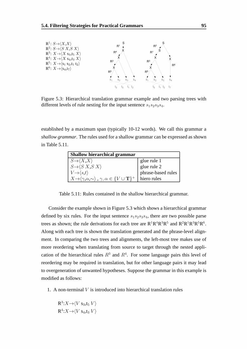
5.4. Filtering Strategies for Practical Grammars 95
R1: S→〈X ,X〉R2: S→〈S X ,S X〉R3: X→〈X s3,t5 X〉R4: X→〈X s4,t3 X〉R5: X→〈s1 s2,t1 t2〉R6: X→〈s4,t7〉
Figure 5.3: Hierarchical translation grammar example and two parsing trees withdifferent levels of rule nesting for the input sentences1s2s3s4.
established by a maximum span (typically 10-12 words). We call this grammar a
shallow grammar. The rules used for a shallow grammar can be expressed as shown
in Table 5.11.
Shallow hierarchical grammarS→〈X,X〉 glue rule 1S→〈S X,S X〉 glue rule 2V→〈s,t〉 phrase-based rulesX→〈γ,α,∼〉 , γ, α ∈ V ∪T+ hiero rules
Table 5.11: Rules contained in the shallow hierarchical grammar.
Consider the example shown in Figure 5.3 which shows a hierarchical grammar
defined by six rules. For the input sentences1s2s3s4, there are two possible parse
trees as shown; the rule derivations for each tree are R1R4R3R5 and R2R1R3R5R6.
Along with each tree is shown the translation generated and the phrase-level align-
ment. In comparing the two trees and alignments, the left-most tree makes use of
more reordering when translating from source to target through the nested appli-
cation of the hierarchical rulesR3 andR4. For some language pairs this level of
reordering may be required in translation, but for other language pairs it may lead
to overgeneration of unwanted hypotheses. Suppose the grammar in this example is
modified as follows:
1. A non-terminalV is introduced into hierarchical translation rules
R3:X→〈V s3,t5 V 〉
R4:X→〈V s4,t3 V 〉

96 Chapter 5. Hierarchical Grammars
2. Rules for lexical phrases are applied toV
R5:V→〈s1 s2,t1 t2〉
R6:V→〈s4,t7〉
These modifications exclude parses in which hierarchical translation rules generate
other hierarchical rules, except at the lexical phrase level. Consequently the left-
most tree of Figure 5.3 cannot be generated andt5t1t2t7 is the only allowable trans-
lation of s1s2s3s4. In this sense, reducing our grammar from a (fully) hierarchical
grammar to a shallow grammar is clearly a form of derivation filtering.
The experiment for Arabic-to-English in Table 5.12 contrasts performance and
speed of a traditional (fully) hiero search space with its reduced shallow grammar.
The decoder is HCP, described in Chapter 4. As can be seen, there is no impact on
BLEU, while translation speed increases by a factor of 7. Of course, these results
are specific to this Arabic-to-English translation task, and do not carry over to other
language pairs, such as Chinese-to-English translation (see Chapter 6). However,
the impact of this search simplification is easy to measure, and the gains can be
significant enough, that it is worth investigation even for languages with complex
long distance movement.
mt02-05- -tune -test
System Time BLEU BLEUHCP - full 14.0 52.1 51.5HCP - shallow 2.0 52.1 51.4
Table 5.12: Translation performance and time (in seconds per word) for full vs.shallow grammars.
5.4.5. Individual Rule Filters
Attempting to further speed up the system, we take our previous shallow
grammar as a baseline and we now filter hierarchical rules individually (not by
class) according to their number of translations, i.e. we limit the number of
translations of each individual source hierarchical phrase. More specifically, for
each fixedγ /∈ T+ (i.e. with at least 1 non-terminal), we define the following filters
over rulesX → 〈γ,α〉:

5.4. Filtering Strategies for Practical Grammars 97
Number of translations (NT). We keep theNT most frequentα’s, i.e. each
γ is allowed to have at mostNT rules.
Number of reordered translations (NRT). We keep theNRT most frequent
α’s with monotonic non-terminals and theNRT most frequentα’s with re-
ordered non-terminals.
Count percentage (CP). We keep the most frequentα’s until their aggregated
number of counts reaches a certain percentageCP of the total counts ofX →
〈γ,∗〉. Someγ’s are allowed to have moreα’s than others, depending on their
count distribution.
Results applying these filters with various thresholds are given in Table 5.13,
including number of rules and decoding time. As shown, all filters achieve at least a
50% speed-up in decoding time by discarding 15% to 25% of the baseline grammar
with 4.2 million rules. Remarkably, performance is unaffected whenapplying the
simpleNT andNRT filters with a threshold of 20 translations. Finally, theCP filter
behaves slightly worse for thresholds of 90% for the same decoding time. For this
reason, we selectNRT=20 as our general filter.
mt02-05- -tune -test
Filter Time Rules BLEU BLEUbaseline 2.0 4.20 52.1 51.4NT=10 0.8 3.25 52.0 51.3NT=15 0.8 3.43 52.0 51.3NT=20 0.8 3.56 52.1 51.4NRT=10 0.9 3.29 52.0 51.3NRT=15 1.0 3.48 52.0 51.4NRT=20 1.0 3.59 52.1 51.4CP=50 0.7 2.56 51.4 50.9CP=90 1.0 3.60 52.0 51.3
Table 5.13: Impact of general rule filters on translation (IBM BLEU), time (in sec-onds per word) and number of rules (in millions).
These findings are quite consistent with Table 5.14, which shows a surprisingly
low hierarchical rule usage for 1-best translations in the initial grammar for the
shallow configuration (Table 5.11). We discovered that onlyaround 3100 different
rules appear in the 1-best translation from a grammar more than one thousand times
bigger. Indeed, a closer look to the rule usage in 1-best alsoreveals that very few

98 Chapter 5. Hierarchical Grammars
Usage Foreign English44 17 X 16 16 X 1532 12 X 12 16 X 1518 X 459 12 12507 12 466 X 840 40399 84017 X 1070 717 X12 X 343 370 X
Table 5.14: Top five hierarchical 1-best rule usage with initial grammar configu-ration for mt02-05-tune. Numbers in source and target parts of each rule map tosource and target words respectively.
synchronous hierarchical rules with the same source phrasetranslate into different
target phrases, and the chosen translations are among the most probable ones in the
grammar extraction.
5.4.6. Revisiting Pattern-based Rule Filters
In order to assess that the greedy search is a valid procedure, in this subsection
we wish to revisit the decisions taken in building our first usable grammar. We first
reconsider whether reintroducing the monotonic patterns (originally excluded as
described in rows ’b’, ’c’, ’d’ in Table 5.9) affects performance. Results are given in
the upper rows of Table 5.15. For all classes, we find that reintroducing these rules
increases the total number of rules substantially, despitethe NRT=20 filter, but leads
to degradation in translation performance.
We next reconsider the mincount threshold values for Nnt.Ne classes 1.3, 2.3,
2.4 and 2.5 originally described in Table 5.9 (rows ’e’ to ’h’). Results under vari-
ous mincount cutoffs for each class are given in Table 5.15 (middle five rows). For
classes 2.3 and 2.5, the mincount cutoff can be reduced to 1 (i.e. all rules are kept)
with slight translation improvements. In contrast, reducing the cutoff for classes
1.3 and 2.4 to 3 and 5, respectively, adds many more rules withno increase in per-
formance. In the latter case there is a decreasing factor of 2, suggesting that the
system is handling plenty overgeneration and spurious ambiguity. We also find that
increasing the cutoff to 15 for class 2.4 yields the same results with a smaller gram-
mar. Finally, we consider further filtering applied to class1.2 with mincount 5 and
10 (final two rows in Table 5.15). The number of rules is largely unchanged, but
translation performance drops consistently as more rules are removed (undergener-
ation).

5.5. Large Language Models and Evaluation 99
mt02-05- -tune -test
Nnt.Ne Filter Time Rules BLEU BLEU
baselineNRT=20 1.0 3.59 52.1 51.42.3 +monotone 1.1 4.08 51.5 51.12.4 +monotone 2.0 11.52 51.6 51.02.5 +monotone 1.8 6.66 51.7 51.21.3 mincount=3 1.0 5.61 52.1 51.32.3 mincount=1 1.2 3.70 52.1 51.42.4 mincount=5 1.8 4.62 52.0 51.32.4 mincount=15 1.0 3.37 52.0 51.42.5 mincount=1 1.1 4.27 52.2 51.51.2 mincount=5 1.0 3.51 51.8 51.31.2 mincount=10 1.0 3.50 51.7 51.2
Table 5.15: Effect of pattern-based rule filters. Time in seconds per word. Rules inmillions.
Based on these experiments, we conclude that applying separate mincount
thresholds to the classes helps to control overgeneration and spurious ambiguity
whilst keeping optimal performance with a minimum size grammar.
5.5. Large Language Models and Evaluation
It is a common strategy in NLP to rerank lattices or n-best lists of translation
hypotheses with one or more steps in which stronger models are used. In this sec-
tion we report results of our shallow hierarchical system with the 2.5 mincount=1
configuration from Table 5.15, after including the following n-best list rescoring
steps.
Large-LM rescoring. We build sentence-specific zero-cutoff stupid-backoff
[Brantset al., 2007] 5-gram language models, estimated using∼4.7B words
of English newswire text, and apply them to rescore each 10000-best list.
Minimum Bayes Risk (MBR). We then rescore the first 1000-best hypotheses
with MBR, taking the negative sentence level BLEU score as the loss function
to minimize[Kumar and Byrne, 2004].
Table 5.16 shows results formt02-05-tune, mt02-05-test, the NIST subsets
from the MT06 evaluation (mt06-nist-nwfor newswire data andmt06-nist-ng

100 Chapter 5. Hierarchical Grammars
mt02-05-tune mt02-05-test mt06-nist-nw mt06-nist-ng mt08HCP+MET 52.2 / 41.6 51.5 / 42.2 48.4 / 43.6 35.3 / 53.2 42.5 / 48.6+rescoring 53.2 / 40.8 52.6 / 41.4 49.4 / 42.9 36.6 / 53.5 43.4 / 48.1
Table 5.16: Arabic-to-English translation results (lower-cased IBM BLEU / TER)with large language models and MBR decoding.
for newsgroup) andmt08, as measured by lowercased IBM BLEU and TER
[Snoveret al., 2006].
The mixed case NIST BLEU for our HCP system onmt08 is 42.5. This is
directly comparable to the official MT08 Constrained Training Track evaluation
results4. It is worth noting that many of the top entries make use of system combi-
nation; the results reported here are for single system translation.
5.6. Shallow-N grammars and Extensions
In this framework it is possible to define many types of grammars, each gram-
mar yielding a different search space. It could be possible to consider filtering in
the parsing stage, for instance according to word spans. We have also seen that lim-
iting the rule nesting to one was a good strategy for the Arabic-to-English task. So
relaxing this constraint for other translation tasks with more language reordering re-
quirements is another strategy worth trying. Or, if a particular problem in the model
is detected, we could addad hocrules to allow the decoder to find the correct hy-
potheses. In the end, the goal is to build efficiently the appropriate search space for
each translation task. In this section we propose the following strategies for more
efficient search space design.
1. Shallow-N grammars. This filtering technique is a natural extension toshal-
low grammars.
2. Low-level phrase concatenation. It augments the search space by allowing
certain hierarchical phrases to be concatenated.
3. Span filtering. This a simple filtering technique applied to the parser.
4See http://www.nist.gov/speech/tests/mt/2008/doc/mt08_official_results_v0.html for full re-sults.

5.6. Shallow-N grammars and Extensions 101
These strategies are described here for coherence with thischapter, although
experimentation will be made withHiFST, hence results and discussion will appear
in the next chapter.
5.6.1. Shallow-N Grammars
In order to face language pairs with greater word reorderingrequirements than
Arabic-to-English, we extend our shallow grammars to a slightly more complex
scheme in which we expect to avoid overgeneration and spurious ambiguity by
adapting rule nesting to the needs of the particular translation task.
A shallow-N translation grammar can be formally defined as :
1. the usual non-terminalS
2. a set of non-terminalsX0, . . . , XN
3. two glue rules:S → 〈XN ,XN〉 andS → 〈S XN ,S XN〉
4. hierarchical translation rules for levelsn = 1, . . . , N :
R: Xn→〈γ,α,∼〉 , γ, α ∈ Xn−1 ∪T+
with the requirement thatα andγ contain at least oneXn−1
5. translation rules which generate lexical phrases:
R: X0→〈γ,α〉 , γ, α ∈ T+
Table 5.17 illustrates the shallow grammars forN = 1, 2, 3. As is clear, with
largerN the expressive power of the grammar grows closer to that of full Hiero.
Shallow grammars are created by a trivial rewriting procedure of the full
grammar. In this context, the added requirement in condition (4) in the definition of
shallow-N grammars is included to avoid spurious ambiguity. To see theeffect of
this constraint, consider the following example with a source sentence ‘s1 s2’ and a
full grammar defined by these four rules:
R1: S→〈X,X〉
R2: X→〈s1 s2,t2 t1〉
R3: X→〈s1 X,X t1〉
R4: X→〈s2,t2〉We can easily rewrite these rules according to a shallow-1 grammar:

102 Chapter 5. Hierarchical Grammars
grammar rules includedS-1 S→〈X1,X1〉 S→〈SX1,SX1〉 glue rules
X0→〈γ,α〉 , γ, α ∈ T+ lexical phrasesX1→〈γ,α,∼〉 , γ, α ∈ X0 ∪T+ hiero rules level 1
S-2 S→〈X2,X2〉 S→〈SX2,SX2〉 glue rulesX0→〈γ,α〉 , γ, α ∈ T+ lexical phrasesX1→〈γ,α,∼〉 , γ, α ∈ X0 ∪T+ hiero rules level 1X2→〈γ,α,∼〉 , γ, α ∈ X1 ∪T+ hiero rules level 2
S-3 S→〈X3,X3〉 S→〈SX3,SX3〉 glue rulesX0→〈γ,α〉 , γ, α ∈ T+ lexical phrasesX1→〈γ,α,∼〉 , γ, α ∈ X0 ∪T+ hiero rules level 1X2→〈γ,α,∼〉 , γ, α ∈ X1 ∪T+ hiero rules level 2X3→〈γ,α,∼〉 , γ, α ∈ X2 ∪T+ hiero rules level 3
Table 5.17: Rules contained in shallow-N grammars forN = 1, 2, 3.
R1: S→〈X1,X1〉
R2: X1→〈s1 s2,t2 t1〉
R3: X1→〈s1 X0,X0 t1〉
R4: X0→〈s2,t2〉
There are two derivations R1R2 and R1R3R4 which yield an identical transla-
tion. However R2 would not be allowed under the constraint introduced here since
there is noX0 in the body of the rule.
5.6.2. Low Level Concatenation for Structured Long Distance
Movement
The basic formulation of shallow-N grammars allows only the upper-level non-
terminal categoryS to act within the glue rule. This can prevent some useful
long-distance movement, as might be needed to translate Arabic sentences in Verb-
Subject-Object order into English. It often happens that the initial Arabic verb re-
quires long distance movement, but the subject which follows can be translated in
monotonic order. For instance, consider the following Romanized Arabic sentence:
TAlb AlwzrA’ AlmjtmEyn Alywm fy dm$q <lY ...
(CALLED) (the ministers) (gathered) (today) (in Damascus)(FOR) ...
where the verb ’TAlb’ must be translated into English so thatit follows the transla-
tions of the five subsequent Arabic words ’AlwzrA’ AlmjtmEynAlywm fy dm$q’

5.6. Shallow-N grammars and Extensions 103
which are themselves translated monotonically. A shallow-1 grammar cannot gen-
erate this movement except in the relatively unlikely case that the five words fol-
lowing the verb can be translated as a single phrase. A more powerful approach is
to define grammars that allow low-level rules to form movablegroups of phrases.
Additional non-terminalsMk are introduced to allow successive generation ofk
non-terminalsXN−1 in monotonic order for both languages, whereK1 ≤ k ≤ K2.
These act in the same manner as the glue rule does in the uppermost level. Apply-
ingMk non-terminals at the N-1 level allows one hierarchical ruleto perform a long
distance movement over the tree headed byMk.
We further refine shallow-N grammars by specifying the allowable values ofk
for the successive productions of non-terminalsXN−1. There are many possible
ways to formulate and constrain these grammars. IfK2 = 1, then the grammar
is equivalent to the previous definition of shallow-N grammars, since monotonic
production is only allowed by the glue rule of level N. IfK1 = 1 andK2 > 1, then
the search space defined by the grammar is greater than the standard shallow-N
grammar as it includes structured long distance movement. Finally, if K1 > 1 then
the search space is different from standard shallow-N as theN level is only used
for long distance movement.
The introduction ofMk non-terminals redefines shallow-N grammars as:
1 the usual non-terminalS
2 a set of non-terminalsX0, . . . , XN
3 a set of non-terminalsMK1, . . . ,MK2 for K1 = 1, 2; K1 ≤ K2
4 two glue rules:S → 〈XN ,XN〉 andS → 〈S XN ,S XN〉
5 hierarchical translation rules for levelN :
R: XN→〈γ,α,∼〉 , γ, α ∈ MK1, . . . ,MK2 ∪T+
with the requirement thatα andγ contain at least oneMk
6 hierarchical translation rules for levelsn = 1, . . . , N − 1:
R: Xn→〈γ,α,∼〉 , γ, α ∈ Xn−1 ∪T+
with the requirement thatα andγ contain at least oneXn−1
7 translation rules which generate lexical phrases:
R: X0→〈γ,α〉 , γ, α ∈ T+

104 Chapter 5. Hierarchical Grammars
Figure 5.4: Movement allowed by two grammars: shallow-1, with K1 = 1, K2 = 3[left], and shallow-2, withK1 = 1,K2 = 3 [right]. Both grammars allow movementof the bracketed term as a unit. Shallow-1 requires that translation within the objectmoved be monotonic while shallow-2 allows up to two levels of reordering.
8 rules which generatek non-terminalsXN−1:
if K1 == 2 :
R: Mk→〈XN−1 Mk−1,XN−1 Mk−1,∼〉 , for k = 3, . . . , K2
R: M2→〈XN−1 XN−1,XN−1 XN−1〉
if K1 == 1 :
R: Mk→〈XN−1 Mk−1,XN−1 Mk−1,∼〉 , for k = 2, . . . , K2
R: M1→〈XN−1,XN−1〉
For example, with a shallow-1 grammar,M3 leads to the monotonic production
of three non-terminals X0, which leads to the production of three lexical phrase
pairs; these can be moved with a hierarchical rule of level 1.This is graphically
represented by the left-most tree in Figure 5.4. With a shallow-2 grammar,M2 leads
to the monotonic production of two non-terminals X1, a movement represented by
the right-most tree in Figure 5.4. This movement cannot be achieved with a shallow-
1 grammar.
5.6.3. Minimum and Maximum Rule Span
We parse the sentence to create the forest that describes thecompletesearch
space using a given grammar, intentionally avoiding any kind of filtering or prun-
ing. But of course, different filtering strategies could be applied here. We propose
two parameters that control the application of hierarchical translation rules in gen-
erating the search space. These two parameters namedhmaxandhminspecify the

5.7. Conclusions 105
maximum and minimum height at which any hierarchical translation rule can be ap-
plied in the CYK grid. In other words, the idea is that a hierarchical rule would only
be applied in cell(x, y) if hmin≤ y ≤hmax. In principle, these filters are expected
to be specially useful for shallow-N grammars, as they are set independently for
each non-terminal category of the grammar. With these experiments we hope to see
whether the span of these rules is significant. Besides the opportunity to speed up
the system, this knowledge could lead to new ideas for searchspace design.
5.7. Conclusions
This chapter has focused on efficient search space design forlarge-scale hi-
erarchical translation. We defined a general classificationof hierarchical rules,
based on their number of non-terminals, elements and their patterns, for refined
extraction and filtering. We have demonstrated that certainpatterns are of much
greater value in translation than others and that separate minimum count filters
should be applied accordingly. Some patterns were found to be redundant or harm-
ful, in particular identical patterns and many monotonic patterns. Moreover, we
show that the value of a pattern is not directly related to thenumber of rules
it encompasses, which can lead to discarding large numbers of rules that are ei-
ther overgenerating or producing spurious ambiguity, and consequently to dramatic
speed improvements. For a large-scale Arabic-to-English task, we show that shal-
low hierarchical decoding is as good as fully hierarchical search and that decod-
ing time is dramatically decreased. In addition, we describe individual rule fil-
ters based on the distribution of translations with furthertime reductions at no
cost in translation scores. This is in direct contrast to recent reported results in
which other filtering strategies lead to degraded performance [Shenet al., 2008;
Zollmannet al., 2008]. Finally, given our initial findings with shallow grammars,
we extend them to a new kind of hierarchical grammars called shallow-N gram-
mars, that attempt to control overgeneration and spurious ambiguity by imposing
a direct constraint to rule nesting. As this constraint filters derivations with longer
distance word reorderings, it should be adapted to each particular translation task.
We also propose low level concatenation and motivate the usefulness of this strat-
egy with an Arabic-English sentence. Finally, we propose tofilter rules by span in
the parser. Experiments for these new strategies have been realized withHiFSTand
thus results and discussion are postponed to the last sections of the next chapter.

106 Chapter 5. Hierarchical Grammars
The experiments reported in this chapter have partially motivated a paper in the
EACL conference[Iglesiaset al., 2009c]. In the next chapter we face the challenge
of implementing a more efficient search algorithm than the hypercube pruning de-
coder.

Chapter 6HiFST: Hierarchical Translation with
WFSTs
Contents6.1. Introduction . . . . . . . . . . . . . . . . . . . . . . . . . . . 107
6.2. From HCP to HiFST . . . . . . . . . . . . . . . . . . . . . . 108
6.3. Hierarchical Translation with WFSTs . . . . . . . . . . . . . 111
6.4. Alignment for MET optimization . . . . . . . . . . . . . . . . 124
6.5. Experiments on Arabic-to-English . . . . . . . . . . . . . . . 133
6.6. Experiments on Chinese-to-English . . . . . . . . . . . . . . 142
6.7. Experiments on Spanish-to-English Translation . . . . .. . 148
6.8. Conclusions . . . . . . . . . . . . . . . . . . . . . . . . . . . . 152
6.1. Introduction
Hypercube pruning decoders, already introduced in Chapter4, rely on hypothe-
ses lists to build the translation search space. Even thoughthis approach is very
effective and has been shown to produce improvements in translation, the reliance
on k-best lists is a limitation that inevitably leads to search errors. In this chapter,
we propose a new search algorithm. Whilst based on a similar hierarchical frame-
work, it uses lattices implemented with weighted finite-state transducers, yielding
more compact and efficient representations of bigger searchspaces and thus more

108 Chapter 6. HiFST: Hierarchical Translation with WFSTs
robust to search errors. By using WFSTs we also benefit from the semiring oper-
ations described in Chapter 2, as this simplifies considerably the implementation.
The outline of this chapter is the following: in Section 6.2 we motivate the shift
from the hypercube pruning decoder (HCP) toHiFST and we discuss the concep-
tual similarities and differences between both decoders. In Section 6.3 we describe
how this decoder can be easily implemented with WFSTs. For this we employ the
OpenFST libraries[Allauzenet al., 2007], as we make use of FST operations such
as composition, epsilon removal, determinization, minimization and shortest-path.
As the use of transducers currently forces us to perform a posterior alignment, we
also discuss two alignment methods for MET optimization in Section 6.4. In Sec-
tions 6.5 and 6.6 we report translation results in Arabic-to-English and Chinese-to-
English translation, respectively, and contrast the performance of lattice-based and
hypercube pruning hierarchical decoding. We will show that, compared to the hy-
percube pruning decoder (HCP), the main advantages are a significant reduction in
search errors, a simpler implementation, direct generation of target language word
lattices, and better integration with other statistical MTprocedures. For Chinese-
to-English and Arabic-to-English, we present contrastiveexperiments with our hy-
percube pruning decoder. We also contrast shallow-N grammars introduced in Sec-
tion 5.6 with full hiero grammars. We also present experiments for low-level phrase
concatenation and the log-probability semiring in Arabic-to-English, and pruning
strategies for Chinese-to-English.
Finally, Section 6.7 shows experiments for the Europarl Spanish-to-English
translation task, after which we conclude.
6.2. From HCP toHiFST
We have already explained that a hypercube pruning decoder works in two
steps (see Chapter 4). In the first step the sentence is parsed. In the second step,
we apply the k-best algorithm with hypercube pruning to build the hypotheses list.
As we traverse the backpointers we build in a bottom-up direction lists for each cell
in the grid containing partial translation hypotheses. These lists could be pruned if
certain conditions are met. At the end, in the topmost cell, we have a list of trans-
lation hypotheses. Figure 6.1 shows an example of what couldbe happening right
after the list for the topmost cell has been built.
In this chapter, we introduceHiFST. Broadly speaking, this decoder will work

6.2. From HCP to HiFST 109
Figure 6.1: HCP builds the search space using lists.
in a very similar fashion to the hypercube pruning decoder. However, rather than
building lists in each cell of the CYK grid, we build a single,minimal word lattice
containing all possible translations of the source sentence span covered by that cell.
In the upper-most cell we have our lattice that spans the whole source sentence and
consequently contains the translation hypotheses.
So in essence, as shows Figure 6.2, what we propose is to throwaway the k-best
lists and use lattices instead, implemented with WFSTs. Themotivation for this is:
1. Lattices are much more compact representations of a spacethan k-best lists.
This translates into bigger search spaces, less search errors and richer list of
hypotheses that can lead to better optimization and rescoring steps.
2. Lattices implemented as WFSTs have the advantage of usingany WFST op-
eration defined on the semiring. This is, we can perform determinization,
minimization, composition, etcetera.
As lattices represent hypotheses lists in a far more compactway, we can state
that by using lattices we are workingin practicewith a search space that is a super
set of the one created by the hypercube pruning decoder. But the underlying ideas
of both decoders are quite the same, as both parse the source sentence and store a
subset of the search space for each cell.
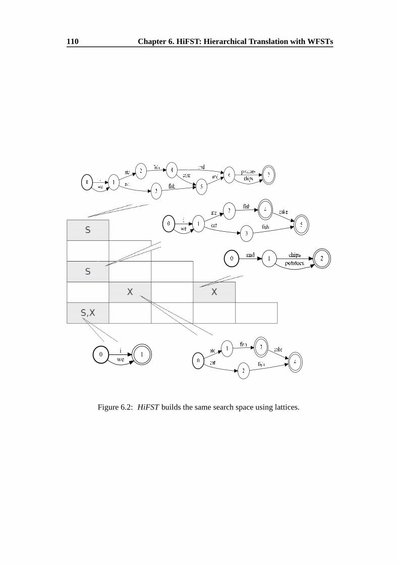
110 Chapter 6. HiFST: Hierarchical Translation with WFSTs
Figure 6.2: HiFST builds the same search space using lattices.

6.3. Hierarchical Translation with WFSTs 111
Figure 6.3: TheHiFST decoder.
We conclude this section by presenting an overview of this new decoder, called
HiFST, depicted in Figure 6.3. Ideally it works in three stages:
1. A parsing algorithm is applied to the source sentence, namely the CYK al-
gorithm, effectively building a grid that stores derivations and required back-
pointers for later use.
2. We build the translation lattice following the backpointers through the CYK
grid. As we will see, for efficiency we do not build in practicethe whole
lattice in one pass. Instead, a much more simpler lattice using pointers to
external lattices is built. In a second pass, the lattice is expanded into the
full lattice containing all the translation hypotheses. Wecall this procedure
delayed translation. Pruning in search may be required in this stage.
3. Once we have the translation lattice for the whole sentence, we apply the
language model. The 1-best (shortest path) corresponds to the hypothesis that
will be evaluated, although keeping the (pruned) translation lattice is useful
for posterior reranking/system combination steps.
In the next section we introduce the equations that govern the decoder. We ex-
plain how it works by following the example from Section 2.3.1. Then we describe
the algorithm, and further refine it with the delayed translation technique, pruning
in search and the deletion rules constraint.
6.3. Hierarchical Translation with WFSTs
The translation system is based on a variant of the CYK algorithm closely
related to CYK+[Chappelier and Rajman, 1998]. Parsing has been described in
Section 2.3. We keep backpointers and employ hypotheses recombination without

112 Chapter 6. HiFST: Hierarchical Translation with WFSTs
discarding rules, unless stated otherwise. The underlyingmodel is a synchronous
context-free grammar consisting of a setR = Rr of rulesRr : N → 〈γr,αr〉 / pr,
with ‘glue’ rules,S → 〈X,X〉 andS → 〈S X,S X〉. If a rule has probabilitypr,
it is transformed to a costcr; here we use the tropical semiring, socr = − log pr.
N denotes any non-terminal (S,X,V , etcetera),N ∈ N. T denotes the terminals
(words), and the grammar builds parse forests based on stringsγ, α ∈ N ∪ T+.
Each cell in the CYK grid is specified by a non-terminal symboland position in the
CYK grid: (N, x, y), which spanssx+y−1x on the source sentence.
In effect, the source language sentence is parsed using a context-free grammar
with rulesN → γ. The generation of translations is a second step that follows
parsing. For this second step, we describe a method to construct word lattices with
all possible translations that can be produced by the hierarchical rules. Construction
proceeds by traversing the CYK grid along the backpointers established in parsing.
In each cell(N, x, y) in the CYK grid, we build a target language word lattice
L(N, x, y). This lattice contains every translation ofsx+y−1x from every derivation
headed byN . These lattices also contain the translation scores on their arc weights.
The ultimate objective is the word latticeL(S, 1, J), which corresponds to all
the analyses that cover the source sentencesJ1 . Once this is built, we can apply a
target language model toL(S, 1, J) to obtain the final target language translation
lattice[Allauzenet al., 2003].
We use the approach of Mohri[2002] in applying WFSTs to statistical NLP. This
fits well with the use of the OpenFST toolkit[Allauzenet al., 2007] to implement
our decoder.
6.3.1. Lattice Construction Over the CYK Grid
In each cell(N, x, y), the set of rule indices used by the parser is denoted
R(N, x, y), i.e. for r ∈ R(N, x, y),N → 〈γr,αr〉 was used in at least one derivation
involving that cell.
For each ruleRr, r ∈ R(N, x, y), we build a latticeL(N, x, y, r). This lattice is
derived from the target side of the ruleαr by concatenating lattices corresponding
to the elements ofαr = αr1...α
r|αr |. If an αr
i is a terminal, creating its lattice is
straightforward. Ifαri is a non-terminal, it refers to a cell(N ′, x′, y′) lower in the
grid identified by the backpointerBP (N, x, y, r, i); in this case, the lattice used is

6.3. Hierarchical Translation with WFSTs 113
Figure 6.4: Translation rules, CYK grid fors1s2s3, and production of the translationlatticeL(S, 1, 3).
L(N ′, x′, y′). Taken together,
L(N, x, y, r) =⊗
i=1..|αr|
L(N, x, y, r, i) (6.1)
L(N, x, y, r, i) =
A(αi) if αi ∈ T
L(N ′, x′, y′) else(6.2)
whereA(t), t ∈ T returns a single-arc acceptor that accepts only the symbolt. The
latticeL(N, x, y) is then built as the union of lattices corresponding to the rules in
R(N, x, y):
L(N, x, y) =⊕
r∈R(N,x,y)
L(N, x, y, r)⊗ cr (6.3)
This slight abuse of notation indicates that the costcr is applied at the path level to
each latticeL(N, x, y, r); the cost can be added to the exit states, for example. This
could as well be done at Equation 6.1.
6.3.1.1. An Example of Phrase-based Translation
In Section 4.3.2 we used a toy example with the following rules:
R1: X → 〈s1 s2 s3,t1 t2〉
R2: X → 〈s1 s2,t7 t8〉
R3: X → 〈s3,t9〉
R4: S → 〈X,X〉

114 Chapter 6. HiFST: Hierarchical Translation with WFSTs
R5: S → 〈S X,S X〉
We will now reuse this example to explain how theHiFST works in practice.
Figure 6.4 depicts the state of the CYK grid after parsing with the rulesR1 toR5 for
translation of sentences1s2s3, and including backpointers, represented as arrows,
from non-terminals to lower-level cells. This is a phrase-based monotone translation
scenario asR1, R2, R3 lack non-terminals, whilstR4, R5 are the glue rules. How to
get to this situation has been explained in Section 2.3.1.
At this point, the system is ready to find translation hypotheses. We are inter-
ested in the upper-most S cell(S, 1, 3), as it represents the search space of translation
hypotheses covering the whole source sentence. The latticeL(S, 1, 3) for this cell
is easy to obtain by using Equations 6.1, 6.2 and 6.3 and traversing backpointers
similarly to the k-best algorithm, explained in Section 4.3.2. Two rules (R4, R5)
are in cell(S, 1, 3), so the latticeL(S, 1, 3) will be obtained by the union of the two
lattices found by the backpointers of these two rules:
L(S, 1, 3) = L(S, 1, 3, 4) ⊕ L(S, 1, 3, 5)
On the other hand,
L(S, 1, 3, 4) = L(X, 1, 3) = L(X, 1, 3, 1) = A(t1)⊗A(t2)
asL(S, 1, 3, 4) is determined byR4, pointing from(S, 1, 3) to (X, 1, 3), which in
turn is determined only byR1, a phrase-based rule. Therefore, we can build it
by concatenations, one arc per each target word in the rule. On the other hand, as
L(S, 1, 3, 5) depends solely onR5, its backpointers leading to(S, 1, 2) and(X, 3, 1),
L(S, 1, 3, 5) is simply a concatenation of two sublattices.
L(S, 1, 3, 5) = L(S, 1, 2)⊗L(X, 3, 1)
Again, lattices in(S, 1, 2) and(X, 3, 1) have to be calculated first. So:

6.3. Hierarchical Translation with WFSTs 115
0
1t 1
3t 7
2
t 2
4t 8
t 9
Figure 6.5: A lattice encoding two target sentences:t1t2 andt7t8t9.
L(S, 1, 2) = L(S, 1, 2, 4) = L(X, 1, 2) = L(X, 1, 2, 2) = A(t7)⊗A(t8)
and
L(X, 3, 1) = L(X, 3, 1, 3) = A(t9)
Substituting,
L(S, 1, 3, 5) = A(t7)⊗A(t8)⊗A(t9)
Finally we can obtain the lattice for(S, 1, 3):
L(S, 1, 3) = (A(t1)⊗A(t2))⊕ (A(t7)⊗A(t8)⊗A(t9))
whereL(S, 1, 3) corresponds to the lattice depicted in Figure 6.5.
6.3.1.2. An Example of Hierarchical Translation
Let us now study the complete scenario by considering three additional rules
R6, R7, R8:

116 Chapter 6. HiFST: Hierarchical Translation with WFSTs
R6: X → 〈s1,t20〉
R7: X → 〈X1 s2 X2,X1 t10 X2〉
R8: X → 〈X1 s2 X2,X2 t10 X1〉
These rules are hierarchical, i.e. they contain non-terminals in the right side.
Figure 6.6 shows the CYK grid for the same sentence, where only hierarchical
derivations have been considered. The reader should note that R7 andR8 share
the source part of the rule and only differ in the target part (i.e. different order of
non-terminals). The goal, once again, is to build a completelattice for(S, 1, 3):
L(S, 1, 3) = L(S, 1, 3, 4) ⊕ L(S, 1, 3, 5)
As we are considering results from the previous example, we can reuse
L(S, 1, 3, 5). For this reasonL(S, 1, 3, 5) is marked with brackets (). Thus, we
only have to calculateL(S, 1, 3, 4):
Figure 6.6: Translation fors1s2s3, with rulesR3, R4, R6,R7,R8.
L(S, 1, 3, 4) = L(X, 1, 3) = L(X, 1, 3, 1) ⊕ L(X, 1, 3, 7)⊕ L(X, 1, 3, 8)
Similarly,L(X, 1, 3, 1) is as obtained for the phrase-based example. So we only
have to find the lattices produced by the two hierarchical rules:

6.3. Hierarchical Translation with WFSTs 117
0
1
t 1
3t 7
5t 2 0
7
t 9
2
t 2
4t 8
6t 1 0
8t 1 0
t 9
t 9
t 2 0
Figure 6.7: A lattice encoding four target sentences:t1t2, t7t8t9, t9t10t20 andt20t10t9.
L(X, 1, 3, 7) = L(X, 1, 1, 6)⊗A(t10)⊗ L(X, 3, 1, 3) = A(t20)⊗A(t10)⊗A(t9)
L(X, 1, 3, 8) = A(t9)⊗A(t10)⊗A(t20)
As expected, the only difference between these two latticesis the order of con-
catenation. This is as easily applied to two naive arcsA(t9) andA(t20) as to full
lattices containing thousands of hypotheses. Indeed, thisprovides a taste of the
power and elegant flexibility of using semiring operations.Finally, the complete
lattice for(S, 1, 3) is:
L(S, 1, 3) = (A(t1)⊗A(t2))⊕
⊕ (A(t20)⊗A(t10)⊗A(t9))⊕ (A(t9)⊗A(t10)⊗A(t20))⊕
⊕ (A(t7)⊗A(t8)⊗A(t9))
whereL(S, 1, 3) now corresponds to the lattice depicted in Figure 6.7.
6.3.2. A Procedure for Lattice Construction
Figure 6.8 presents the algorithm used inHiFST to build the lattice for every
cell. The algorithm uses memoization: if a lattice for a requested cell already exists,

118 Chapter 6. HiFST: Hierarchical Translation with WFSTs
it is returned (line 2); otherwise it is constructed via Equations 6.1, 6.2 and 6.3.
For every rule, each element of the target side (lines 3,4) ischecked as terminal or
non-terminal (Equation 6.2). If it is a terminal element (line 5), a simple acceptor
is built. If it is a non-terminal (line 6), the lattice associated to its backpointer is
returned (lines 7 and 8). The complete latticeL(N, x, y, r) for each rule is built by
Equation 6.1 (line 9). The latticeL(N, x, y) for this cell is then found by union of all
the component rules (line 10, Equation 6.3); this lattice isthen reduced by standard
WFST operations (lines 11,12,13). It is important at this point to remove any epsilon
arcs which may have been introduced by the various WFST union, concatenation,
and replacement operations described in Section 2.2.2, as operations over finite-state
machines with too many epsilons may lead to memory explosion.
1 function buildFst(N,x,y)2 if ∃ L(N, x, y) returnL(N, x, y)3 for r ∈ R(N, x, y), Rr : N → 〈γ,α〉4 for i = 1...|α|5 if αi ∈ T , L(N, x, y, r, i) = A(αi)6 else7 (N ′, x′, y′) = BP (αi)8 L(N, x, y, r, i) = buildFst(N ′, x′, y′)9 L(N, x, y, r)=
⊗
i=1..|α|L(N, x, y, r, i)
10 L(N, x, y) =⊕
r∈R(N,x,y) L(N, x, y, r)
11 fstRmEpsilonL(N, x, y)12 fstDeterminizeL(N, x, y)13 fstMinimizeL(N, x, y)14 returnL(N, x, y)
Figure 6.8: Recursive Lattice Construction.
6.3.3. Delayed Translation
Equation 6.2 leads to the recursive construction of lattices in upper-levels of the
grid through the union and concatenation of lattices from lower levels. If Equa-
tions 6.1 and 6.3 are actually carried out over fully expanded word lattices, the
memory required by the upper lattices will increase exponentially.
To avoid this, we use special arcs that serve as pointers to the low-level lattices.
This effectively builds a skeleton of the desired lattice and delays the creation of
the final word lattice until a single replacement operation is carried out in the top
cell (S, 1, J). To make this exact, we define a functiong(N, x, y) that returns a

6.3. Hierarchical Translation with WFSTs 119
unique tag for each lattice in each cell, and use it to redefineEquation 6.2. With the
backpointer(N ′, x′, y′) = BP (N, x, y, r, i), these special arcs are introduced as:
L(N, x, y, r, i) =
A(αi) if αi ∈ T
A(g(N ′, x′, y′)) else(6.4)
The resulting latticesL(N, x, y) are a mix of target language words and lattice
pointers (Figure 6.9, top lattice). However, each still represents the entire search
space of all translation hypotheses covering the span.
At the upper-most cell, the latticeL(S, 1, J) contains pointers to lower-level lat-
tices. A single FST replace operation[Allauzenet al., 2007] recursively substitutes
all pointers by their lower-level lattices until no pointers are left, thus producing the
complete target word lattice for the whole source sentence.The use of the lattice
pointer arc was inspired by the ‘lazy evaluation’ techniques developed by Mohri
et al. [2000]. Its implementation uses the infrastructure provided by the OpenFST
libraries for delayed composition, etc.
Figure 6.9: Delayed translation during lattice construction.
As an example, consider a hypothetic situation depicted in Figure 6.9, in which
we are running the lattice construction. We have built a lattice for one of the cells of

120 Chapter 6. HiFST: Hierarchical Translation with WFSTs
row 1 in the CYK grid (L1). At some point in row3 we are building a new latticeL3
that requires through various hierarchical rules the lowerlatticeL1. This means that
L1 could be replicated more than once intoL3. It is easy to foresee the potential for
state exponential growth, as lattices at a higher rowj will probably require bothL3
andL1, which in turn will feed even higher rows, etcetera. To solvethis problem,
we use a single arc inL3 that points toL1, effectivelydelayingthe procedure of
building pure translation hypotheses until the expansion.This keeps under control
the size of lattices as we go up the CYK grid during the latticeconstruction.
Importantly, operations on these cell lattices — such as lossless size reduction
via determinization and minimization — can still be performed. Owing to the ex-
istence of multiple hierarchical rules which share the samelow-level dependen-
cies, these operations can greatly reduce the size of the skeleton lattice; Figure 6.10
shows the effect on the translation example. As stated, sizereductions can be sig-
nificant. However, not all redundancy is removed, since duplicate paths may arise
through the concatenation and union of sublattices with different spans.
One interesting issue is where to use and wherenot to use pointer arcs. As
explained in Chapter 2, several WFST operations are quite efficient due to the use
of epsilon arcs. Unfortunately, combining carelessly these operations introduces an
excessive number of epsilon arcs that very easily lead to intractable lattices. In many
cases, removing epsilons is enough. But the expansion is a single operation that
recursively traverses all the arcs substituting pointers to lower lattices by adding at
least two epsilons per substitution1. So, the issue is not only about making the lattice
construction fast, but delivering a tractable skeleton forposterior steps. We decide
which cell lattice will be replaced by a single arc dependingon the non-terminal
this cell is associated to. The reader should note that, as a rule of thumb, theS
cell lattices should never be replaced by pointer arcs, as they are used recursively
many times for each translation hypothesis. A lattice construction doing so would
return a minimal FST of two states binded by one single pointer arc, from which
the complete search space lattice (possibly with millions of derivations) must be
created, including at least twice as many epsilons as glue rules used within each
derivation.
1See Section 2.3.3. There could be more than two epsilons if there is more than one finite state.

6.3. Hierarchical Translation with WFSTs 121
0
1t1
2g(X,1,2)
3g(X,1,1)
5
g(X,3,1)
7
t2
g(X,3,1)
4t10
6t10
g(X,3,1)
g(X,1,1)
0
3g(X,1,1)
2g(X,1,2)
1
t1
4
g(X,3,1)
t10
6
g(X,3,1)
t2
5t10
g(X,1,1)
Figure 6.10: Delayed translation WFST with derivations from Figure 1 and Figure2 before [t] and after minimization [b].
6.3.4. Pruning in Lattice Construction
As introduced in Section 5.3, there are two pruning strategies we can apply:Full
PruningandPruning in Search. We now explain how each strategy is implemented
in HiFST.
6.3.4.1. Full Pruning
The final translation latticeL(S, 1, J) can grow very large after the pointer arcs
are expanded. We therefore apply a word-based language model, via WFST com-
position, and perform likelihood-based pruning[Allauzenet al., 2007] based on the
combined translation and language model scores. For directevaluation we simply
need the 1-best hypotheses; for posterior reranking steps bigger search spaces are
required. As stated previously, this kind of pruning will strictly take out the worst
hypotheses of the search space. In this sense it is predictable and any undergenera-
tion problems it could produce is due to an incorrect search space modeling.

122 Chapter 6. HiFST: Hierarchical Translation with WFSTs
6.3.4.2. Pruning in Search
Pruning can also be performed on sublattices during search.This is an undesired
situation in which the search space grows so big that the onlyway to handle it with
our hardware resources is to discard hypotheses, at the riskof search errors that will
lead to spurious undergeneration problems, very difficult to control.
In order to have as much control as possible over this situation,HiFST follows
the strategy described next. We define a condition demandingthat certain events,
when running the decoder, must occur jointly in order to trigger the search pruning
procedure on the minimized latticeL(N, x, y). These events are three:
1. The specific non-terminalN accepts pruning.
2. The cell(N, x, y) spans a minimum number of words.
3. The number of states of the minimized lattice exceeds a minimum threshold.
For example, a conditionX, 5, 1000 means that a transducer spanning five
source words from anX cell will be pruned if it has1000 states or more. We
typically add one more parameter to set the likelihood pruning, i.e. X, 5, 1000, 9
would prune hypotheses with a cost that exceeds9 respect to the 1-best hypothesis.
The same non-terminal may accept different configurations.For instance, we could
trigger pruning for a fully hierarchical grammar ifX cell lattices spanning2 words
exceed 1000 states,X cell lattices spanning5 words exceed 10000 states andX cell
lattices spanning10 words exceed 100000 states. For grammars with more types of
non-terminals, more possible configurations are available.
This offers a fine-grained strategy for pruning, with the objective of no more
than doing it in order to obtain a feasible output to compute.
In terms of implementation, we expand any pointer arcs and apply a word-based
language model via composition. The resulting lattice is then reduced by likelihood-
based pruning, after which the language model scores are removed, as shown in
Figure 6.11.
Interestingly, pruning in search not only risks performance by means of search
errors. These can be more or less controlled with an adequatepruning configura-
tion. But it has a severe impact on speed. If this procedure isfrequently triggered,
decoding times will increase considerably. Conversely, ifpruning in search is not
needed, the translation stage could be quite fast, unless the final lattice is so big that

6.3. Hierarchical Translation with WFSTs 123
1 function pruneInSearch(L)2 fstReplaceL3 ApplyLM L4 fstPruneL5 RemoveLML6 returnL
Figure 6.11: Pseudocode for Pruning in Search.
composing and posterior pruning/shortest-path is too slow. We will discuss several
pruning experiments in Section 6.6.3.
6.3.5. Deletion Rules
It has been experimentally found that statistical machine translation systems
tend to benefit from allowing a small number of deletions. In other words, allowing
some input words to be ignored (untranslated, or translatedto NULL) can improve
translation output. For this purpose, we want to add to our grammar a deletion rule
for each source-language word, i.e. synchronous rules withthe target side set to a
special tag identifying the null word.
In practice, this represents a huge increase in the search space as any number of
consecutive words can be left untranslated. To control thisundesired situation, we
apply two strategies:
1. Inspired by the shallow grammar approach, we insert the deletion rules in such
a way that they will not be used as non-terminals for higher hierarchical rules.
In other words, each deletion rule is generated by a non-terminal that can
only feed the high glue rule used to buildS by non-lexicalized non-terminal
concatenation. Table 6.1 shows both full and shallow hierarchical grammars
modified to allow deletion rules in this way2.
2. We limit the number of consecutive deleted words. This is done by standard
composition with an unweighted transducer that maps any word to itself, and
up to k NULL tokens toǫ arcs. In Figure 6.12 this simple transducer for
k = 1 andk = 2 is drawn. Composition of the lattice in each cell with this
transducer filters out all translations with more thank consecutive deleted
words.
2Out-of-vocabulary words (OOVs) are coded in a very similar way.

124 Chapter 6. HiFST: Hierarchical Translation with WFSTs
Hiero Hiero ShallowV → 〈γ,α〉 X → 〈γs,αs〉X → 〈V ,V 〉 X → 〈V ,V 〉
X → 〈si,NULL〉 V → 〈s,t〉,X → 〈si,NULL〉γ, α ∈ (X ∪T)+ s, t ∈ T+; γs, αs ∈ (V ∪T)+
Table 6.1: Full and shallow grammars, including deletion rules.
word:wordNULL:ǫ
word:word
10word:word
NULL:ǫ
word:word
word:word
NULL :ǫ102
Figure 6.12: Transducers for filtering up to one [left] or two[right] consecutivedeletions.
6.3.6. Revisiting the Algorithm
Taking into account previous subsections, we now show in Figure 6.13 the ex-
tended recursive algorithm for lattice construction, which includes pruning, delayed
translation and deletion rules. To be more precise, after minimizing the lattice we
filter out consecutive nulls (line 14). If the joint conditions (i.e. non-terminal, num-
ber of states threshold and minimum word span) for search pruning are met (sp-
conditions, line 15), then we trigger the pruning procedurein Figure 6.11. Finally,
this lattice is stored and the function returns a trivial lattice consisting of two states
binded by a pointer arc (pointing to the stored lattice), if allowed for this cell (pa-
conditions, line 16). If not, the complete lattice is returned. The output is a lattice,
which opens up the possibility of applying more powerful models in rescoring (see
Sections 6.5, 6.6, and 6.7).
In Figure 6.14 we provide the reader with the global perspective for a full trans-
lation of the sentence.
6.4. Alignment for MET optimization
As introduced in Section 3.4.2, MET optimization[Och, 2003] is typically used
within maximum entropy frameworks to optimize a vector withthe scaling factors
assigned to each feature,λ = (λ1, . . . , λn). If we are not going to apply this opti-
mization step, the most efficient way in translation is to keep only one single cost,

6.4. Alignment for MET optimization 125
1 function buildFst(N,x,y)2 if ∃ L(N, x, y) returnL(N, x, y)3 for r ∈ R(N, x, y), Rr : N → 〈γ,α〉4 for i = 1...|α|5 if αi ∈ T , L(N, x, y, r, i) = A(αi)6 else7 (N ′, x′, y′) = BP (αi)8 L(N, x, y, r, i) = buildFst(N ′, x′, y′)9 L(N, x, y, r)=
⊗
i=1..|α|L(N, x, y, r, i)
10 L(N, x, y) =⊕
r∈R(N,x,y) L(N, x, y, r)
11 fstRmEpsilonL(N, x, y)12 fstDeterminizeL(N, x, y)13 fstMinimizeL(N, x, y)14 filterConsecutiveNullsL(N, x, y)15 if (sp-conditions) pruneInSearchL(N, x, y)16 if (pa-conditions) return pointer toL(N, x, y)17 returnL(N, x, y)
Figure 6.13: Recursive lattice construction, extended.
1 function HiFst(sentence)2 parsesentence→ CYK grid with topmost cell(S, 1, J)3 L =buildFst(S, 1, J)4 expandLatticeL5 ApplyLM L6 fstPruneL7 returnL
Figure 6.14: Global pseudocode forHiFST.
obtained by summing all the feature costs multiplied by their respective scaling fac-
tors. For optimization we must keep a vector of costs representing each individual
feature contribution to the overall score. Ideally, for optimization we would like
to extend our decoder to be able to do this in one single pass. We would like to
build a transducer that represents the mapping from all possible rule derivations to
all possible translations — in the same conditions as the decoding explained above,
and containing costs vectors instead of single costs. We would even be content with
single costs, as if we know the derivations we can still recover this information. But
creating this transducer, which maps derivations to translations, is not feasible for
large translation search spaces. The solution is to make a second pass thatalignsto
a translation reference provided by the first pass decoding.Such a strategy has also
been followed for other WFST-based translation systems[Blackwoodet al., 2008].

126 Chapter 6. HiFST: Hierarchical Translation with WFSTs
This is depicted in Figure 6.15.
Figure 6.15: Alignment is needed to extract features for optimization.
In Section 3.6 we said that a translation unit coincides witha rule of synchronous
context-free grammars. We now express such a rule as:
N → γ, α, c,∼
with N ∈ N; γ,α ∈ N ∪ T, andc = (c1, ...cK) is a vector of costs that depend
on each particular translation unit,K = |c|.
Assume that we are given a source sentences and a target sentencet, previously
suggested by our decoder with costcst. We carry out bilingual decoding under the
hiero grammar using the translation sentencet as a constraint. This produces the
set oftreesthat can generate the sentence pairs, t. This is the standard alignment
procedure: we already know the translation and its overall cost, but we wish to find
out more details (i.e. feature costs) concerning the particular tree that generated it.
Each treeT is defined uniquely by a derivation of rulesRr1 , . . . , Rrn and thus the
final cost vector (without scaling) for this tree can be defined as in Equation 6.5:
cT =∑
∀rj
crj (6.5)
wherej iterates over all rules of this particular derivation. These final cost vec-
tors are used to train theλ within the maximum entropy framework. Formally ex-
pressed, for a given set of scaling factorsλ the overall costc for a given derivation
is obtained, as shows Equation 6.6, with the scalar product of λ and the vector of

6.4. Alignment for MET optimization 127
costs corresponding to the features of this derivation. Ideally, c = cst.
c = λ · cT =
K∑
i=1
λicTi =
K∑
i=1
λi
∑
∀rj
crji (6.6)
In the general case, we use as a reference a fixed number of possible translation
hypotheses (i.e. typically 1000 hypotheses). Typically, the aligner will find the best
derivation that leads to a reference translation hypothesis, which is the derivation
we are looking for unless the best derivation has been discarded in the decoder due
to search errors in translation. Having found in this way allthe feature costs, we can
proceed to optimize. In the context of hierarchical decoding, the MET optimization
problem[Och, 2003] consists of searching a new vectorλ′, attempting to change
the costs for each treeT , aiming to reorder translation hypotheses. Typically, the
goal is to align the combined models to the BLEU metric, whichis our case.
We now describe two alternative implementations of the aligner.
6.4.1. Alignment via Hypercube Pruning decoder
By default, HCP is already able to carry through the originalcost vectors, needed
for MET optimization. So we modified our hypercube pruning decoder in order
to work in alignment mode. The hypercube size is set to infinite, i.e. no prun-
ing at all is required. The decoding process is guided by means of a suffix array
search[Manber and Myers, 1990] that provides access to every possible valid sub-
string within the reference translations. This allows to discard partial translation
hypotheses that are not substrings of the complete reference sentences. The suffix
array search is a standard solution typically used to searchpartial substrings within
a big corpus. It is very efficient as for initialization and memory usage: only an
extra set of indices is required apart from the translation references. Figure 6.16
provides an overview of how it is implemented.
Due to the constrained search space, the aligner makes no search errors. This
guarantees that the best derivation for the aligned hypothesis is always obtained. If
the decoder has produced, due to a search error, the same output with a worst deriva-
tion (i.e. with a worst cost), there will be a cost mismatch that could lead to reranked
hypotheses. This could harm the MET procedure. In general, special care has to be
taken to ensure that both the aligner and the decoder use the same constraints. For
instance, ifHiFST only allows to delete one consecutive word but the hypercube

128 Chapter 6. HiFST: Hierarchical Translation with WFSTs
pruning decoder does not have the same constraint, it will eventually produce alter-
native derivations with two or more consecutive words deleted. If they yield a better
cost these will be chosen with the risk of harming the MET optimization.
For full hierarchical translation, the alignment step is roughly 8 times faster
than decoding. In contrast, alignment and decoding yield similar speeds for shallow
grammars.
Figure 6.16: An example of a suffix array used on one referencetranslation. Wordsare mapped to an array of indices by alphabetical order. Search of word sequencesis performed with a binary search. For instance, the search will find hypothetictranslation candidates ‘boy’, ‘boy ate’ and ‘boy ate potatoes’ at index3, but will notfind a translation candidate ‘boy ate fish and chips’.
6.4.2. Alignment via FSTs
In this subsection we propose a solution to the alignment problem using FSTs.
Consider again the example in Section 6.3.1 (Figures 6.4 and6.6). Only one deriva-
tion leads to the target sentencet20t10t9: R4R7R6R3. Figure 6.17 shows a trans-
ducer that encodes simultaneously this rule derivation (input language of the trans-
ducer) and its translation (output language). More generally, we can represent the
mappings from rule derivations to translation sequences asa transducer. Figure 6.18
shows two different derivations that lead to the same translation.
In order to construct this, we introduce two modifications into lattice construc-
tion over the CYK grid described in Section 6.3.1:
1. In each cell we build transducers that map rule derivations to the translation

6.4. Alignment for MET optimization 129
R4 : ǫ R3 : t9ǫ : t10R7 : ǫ R6 : t2010 32 54
Figure 6.17: FST encoding simultaneously a rule derivationR4R7R6R3 and thetranslationt20t10t9.
hypotheses they produce. In other words, the transducer output strings are
all possible translations of the source sentence span covered by that cell; the
input strings are all the rule derivations that generate those translations. The
rule derivations are expressed as sequences of rule indicesr given the set of
rulesR = Rr.
2. As these transducers are built they are composed with acceptors for subse-
quences of the reference translations so that any translations not present in
the given set of reference translations are removed. In effect, this replaces
the general target language model used in translation with an unweighted au-
tomaton that accepts only substrings belonging to the translation reference. It
is functionally equivalent to the suffix array solution proposed for alignment
with the modified hypercube pruning decoder.
For alignment, Equations 6.1 and 6.2 are redefined as:
L(N, x, y, r) = AT (r, ǫ)⊗
i=1..|αr|
L(N, x, y, r, i) (6.7)
L(N, x, y, r, i) =
AT (ǫ, αi) if αi ∈ T
L(N ′, x′, y′) otherwise(6.8)
whereAT (r, t), Rr ∈ R, t ∈ T returns a single-arc transducer that accepts the
symbolr in the input language (rule indices) and the symbolt in the output language
(target words). The weight assigned to each arc is the same inalignment as in
translation. With these definitions the goal latticeL(S, 1, J) is now a transducer
with rule indices in the input symbols and target words in theoutput symbols. A
simple example is given in Figure 6.18 where two rule derivations for the translation
t5t8 are represented by the transducer.

130 Chapter 6. HiFST: Hierarchical Translation with WFSTs
R5 : ǫ R6 : t5
R3 : t5
R1 : ǫ
R1 : ǫR2 : ǫ R4 : t8
ǫ : t8
1
0
32
5
4
76
Figure 6.18: FST encoding two different rule derivationsR2R1R3R4 andR1R5R6,for the same translationt5t8. The input sentence iss1s2s3 while the grammar con-sidered here contains the following rules: R1: S→〈X,X〉, R2: S→〈S X,S X〉 , R3:X→〈s1,t5〉, R4: X→〈s2 s3,t8〉, R5: X→〈s1 X s3,X t8〉 and R6: X→〈s2,t5〉.
t1
t3
t2t4
1
0 32
ǫt2ǫ
t3
ǫ
t4
ǫt1
1
0 32
4
Figure 6.19: Construction of a substring acceptor. An acceptor for the stringst1t2t4andt3t4 [left] and its substring acceptor [right]. In alignment thesubstring acceptorcan be used to filter out undesired partial translations via standard FST compositionoperations.

6.4. Alignment for MET optimization 131
6.4.2.1. Using a Reference Acceptor
As we are only interested in those rule derivations that generate the given target
references, we can discard non-desired translations via standard FST composition
of the lattice transducer with the given reference acceptor. In principle, this would
be done in the upper-most cell of the CYK, once the complete source sentence has
been covered. However, keeping track of all possible rule derivations and all pos-
sible translations until the last cell may not be computationally feasible for many
sentences. It is more desirable to carry out this filtering inlower-level cells while
constructing the lattice over the CYK grid so as to avoid storing an increasing num-
ber of undesired translations and derivations in the lattice. To do so we compose
cell lattices with a reference acceptor to cut off translations not containing strictly
substrings of the references. We follow a similar strategy to that ofsearch pruning:
any cell lattice is susceptible of being composed with the reference acceptor to cut
off translations not containing strictly substrings of thereferences. We use as joint
triggers for this procedure the non-terminal, the number ofstates and the word span
size.
As for the reference lattice itself, it is just an unweightedautomaton that ac-
cepts all possible substrings of each target reference string. For instance, given the
reference stringt1t2 . . . tJ , we build an acceptor for all substringsti . . . tj , where
1 ≤ i ≤ j ≤ J . This reference acceptor will accept correctly the complete refer-
ence strings at the uppermost cell if the start and the end of the sentence are marked
with unique tags that cannot appear in any other position of the sentence. Other-
wise, in the upper-most cell we would have to compose with a reference acceptor
that only accepts complete reference strings. Given a lattice of target references, the
unweighted substring acceptor is built as follows:
1. change all non-initial states into final states
2. add one initial state and addǫ arcs from it to all other states
Figure 6.19 shows an example of a substring acceptor for the two references
t1t2t4 andt3t4. The substring acceptor also accepts an empty string, accounting for
those rules that delete source words,i.e., translate into NULL. In some instances the
final composition with the reference acceptor might return an empty lattice. If this
happens there is no rule sequence in the grammar that can generate the given source
and target sentences simultaneously.

132 Chapter 6. HiFST: Hierarchical Translation with WFSTs
6.4.2.2. Extracting Feature Values from Alignments
The term∑
∀rjcrji from Equation 6.6 is the contribution of theith feature to
the overall translation score for that parse. These are the quantities that need to be
extracted from alignment lattices for use in optimization procedures such as MET
for estimation of each scaling factorλi.
So far, the procedure described in this section produces alignment lattices with
scores consistent with the total parse score. Further stepsmust be taken to factor
this overall score to identify the contribution due to individual features or transla-
tion rules. We introduce a rule acceptor that accepts sequences of rule indices, such
as the input sequences of the alignment transducer, and assigns weights in the form
of K-dimensional vectors. Each component of the weight vector corresponds to the
feature value for that rule. Arcs have the form0Rr/wr
−→ 0 wherewr = [cr1, . . . , crK ].
An example of composition with this rule acceptor is given inFigure 6.20 to il-
lustrate how feature scores are mapping to components of theweight vector. The
same operations can be applied to the (unweighted) alignment transducer on a much
larger scale to extract the statistics needed for minimum error rate training.
r/[cr1, . . . , crK ]
0
R5 : ǫ R6 : t5
R3 : t5
R1 : ǫ
R1 : ǫR2 : ǫR4 : t8/[c
T11 . . . cT1K ]
ǫ : t8/[cT21 . . . cT2K ]
1
0
32
5
4
76
Figure 6.20: One arc from a rule acceptor that assigns a vector of K featureweights to each rule [top] and the result of composition withthe transducer ofFigure 6.18 (after weight-pushing) [bottom]. The components of the finalK-dimensional weight vector agree with the feature weights ofthe derivation relatedto a specific parse tree, e.g.cT1i = c2i + c1i + c3i + c4i for i = 1 . . .K.
In HiFST, given the upper most cell alignment transducer obtained as described
in the previous section, this is simply achieved by replacing each arc weight with a
vector of weights; for instance, via composition with a ruleacceptor that assigns a

6.5. Experiments on Arabic-to-English 133
vector ofK feature costs[cr1, cr2, . . . , c
rK ] to each rule indexr. Figure 6.21 shows an
example of this rule acceptor when considering only three rule indices.
0
AAAAAAAAAAAAAAA
BBBBBBBBBBBBBBB
CCCCCCCCCCCCCCC3/[c31, c32, . . . , c
3K ]
2/[c21, c22, . . . , c
2K ]
1/[c11, c12, . . . , c
1K ]
Figure 6.21: A rule acceptor that assigns a vector ofK feature weights to each rule.
FST projection to the output symbols can be used then to discard the rule indices,
so that the resulting lattice is an acceptor containing all the paths that generated any
of the reference translationswith separate feature contributions, as expressed by the
vectors of weights associated to each arc.
Typically, MET optimization is performed considering the best derivation that
generated each reference translation. This is obtained by determinizing the acceptor
described above in the tropical semiring,i.e. finding the Viterbi probability associ-
ated to each distinct translation. However, in this framework alternative approaches
could be followed, such as determinizing in the log semiring, i.e. using marginal
probabilities instead. It should be also noted that, in order to apply determiniza-
tion correctly, each weight must be scaled appropriately, so we still obtain the same
overall weight for each derivation. But applying or removing these scaling factors
is a fairly trivial operation within the OpenFST framework.
6.5. Experiments on Arabic-to-English
Consistently with experiments in Chapter 4, In this sectionwe report experi-
ments on the NIST MT08 (and MT09) Arabic-to-English translation task. For trans-
lation model training we use all allowed parallel corpora inthe NIST MT08 Arabic
track (∼150M words per language). Alignments are generated over theparallel data
with MTTK [Deng and Byrne, 2006; Deng and Byrne, 2008]. The following fea-
tures are extracted and used in translation: target language model, source-to-target
and target-to-source phrase translation models, word and rule penalties, number of
usages of the glue rule, source-to-target and target-to-source lexical models, and

134 Chapter 6. HiFST: Hierarchical Translation with WFSTs
three rule count features inspired by Bender et al.[2007]. The initial English lan-
guage model is a 4-gram estimated over the parallel text and a965 million word
subset of monolingual data from the English Gigaword Third Edition. In addition
to the MT08 set itself, we use a development setmt02-05-tuneformed from the odd
numbered sentences of the NIST MT02 through MT05 evaluationsets; the even
numbered sentences form the validation setmt02-05-test. Themt02-05-tuneset has
2,075 sentences. It contains newswire, with four references. BLEU scores are ob-
tained withmteval-v133. Standard MET[Och, 2003] iterative parameter estimation
under IBM BLEU is performed on the corresponding development set extracting
features as explained in previous sections.
After translation with optimized feature weights, we carryout the two following
rescoring steps.
Large-LM rescoring. We build sentence-specific zero-cutoff stupid-backoff
[Brantset al., 2007] 5-gram language models, estimated using∼4.7B words
of English newswire text, and apply them to rescore either 10000-best lists
generated by HCP or word lattice generated by HiFST.
Minimum Bayes Risk (MBR). We rescore the first 1000-best hypothe-
ses with MBR[Kumar and Byrne, 2004], or the lattice with Lattice MBR
(LMBR) [Trombleet al., 2008], taking the negative sentence level BLEU
score as the loss function.
6.5.1. Contrastive Experiments with HCP
We now contrast our two hierarchical phrase-based decoders. The first decoder,
HCP, is the hypercube pruning decoder implemented as described in Chapter 4. The
second decoder, HiFST, is the lattice-based decoder implemented with weighted
finite-state transducers as described in the previous sections. For the HCP system,
feature contributions are logged during decoding and MET isperformed afterwards.
For theHiFSTsystem, we obtain a k-best list from the translation latticeand extract
each feature score with HCP in alignment mode, as described in Section 6.4.1.
The grammar is built following the filtering strategies explained in Section 5.4.
We translate Arabic-to-English with shallow hierarchicaldecoding as defined in
Table 5.11,i.e. only phrases are allowed to be substituted into non-terminals.
3See ftp://jaguar.ncsl.nist.gov/mt/resources/mteval-v13.pl.

6.5. Experiments on Arabic-to-English 135
decoder mt02-05-tune mt02-05-test mt08a HCP 52.5 51.9 42.8
+5g 53.4 52.9 43.5+5g+MBR 53.6 53.0 43.6
b HiFST 52.5 51.9 42.8+5g 53.6 53.2 43.9+5g+MBR 54.0 53.7 44.2+5g+LMBR 54.3 53.7 44.8
Decoding time in secs/word: 1.1 for HCP; 0.5 for HiFST.
Table 6.2: Contrastive Arabic-to-English translation results (lower-cased IBMBLEU) after first-pass decoding and subsequent rescoring steps. Decoding timereported formt02-05-tune. Both systems are optimized using MET over the k-bestlists generated by HCP.
The hypercube pruning decoder employs k-best lists of depthk=10000. Using
deeper lists results in excessive memory and time requirements. In contrast, the
WFST-based decoder, HiFST, requires no search pruning during lattice construction
for this task and the language model is not applied until the lattice is fully built at
the upper-most cell of the CYK grid.
Table 6.2 shows results formt02-05-tune, mt02-05-testandmt08, as measured
by lowercased IBM BLEU4) and TER[Snoveret al., 2006]. MET parameters are
optimized for the HCP decoder. As shown in rows ‘a’ and ‘b’, results after MET
are comparable.
6.5.1.1. Search Errors
Since both decoders use exactly the same features, we can measure their search
errors on a sentence-by-sentence basis. A search error is assigned to one of the
decoders if the other has found a hypothesis with lower cost.Formt02-05-tune, we
find that in 18.5% of the sentencesHiFST finds a hypothesis with lower cost than
HCP. In contrast, HCP never finds any hypothesis with lower cost for any sentence.
This is as expected: theHiFST decoder requires no pruning prior to applying the
language model, so the search is exact. This means that for this translation task
HiFST is able to avoid spurious undergeneration due to search errors.
4It should be noted that scores in Chapter 5 have been obtainedwith a different version of thebleu scorer. This accounts for the difference with HCP scores in Table 5.16.

136 Chapter 6. HiFST: Hierarchical Translation with WFSTs
6.5.1.2. Lattice/k-best Quality
Rescoring results are different for hypercube pruning and WFST-based de-
coders. Whereas HCP improves by 0.9 BLEU,HiFST improves over 1.5 BLEU.
Clearly, search errors in HCP not only affect the 1-best output but also the quality
of the resulting k-best lists. For HCP, this limits the possible gain from subse-
quent rescoring steps such as large language models and MBR.Importantly, using
LMBR [Trombleet al., 2008] as a scoring step on top ofHiFST yields an improve-
ment on all sets respect to MBR. This is yet another piece of evidence of how k-best
list implementations are easily surpassed by lattices due to its efficient, more com-
pact and richer representation of the search space.
6.5.1.3. Translation Speed
HCP requires an average of 1.1 seconds per input word.HiFST cuts this time
by half, producing output at a rate of 0.5 seconds per word. Itproves much more
efficient to process compact lattices containing many hypotheses rather than to inde-
pendently processing each one of them in k-best form. Again,this is due toHiFST
being able to avoid pruning in search: for both decoders thisis a costly operation.
The mixed case NIST BLEU for theHiFST system onmt08 is 42.9. This is
directly comparable to the official MT08 Constrained Training Track evaluation
results5. As in the previous chapter, the reader should note that manyof the top
entries make use of system combination, whilst the results reported here are for
single system translation.
6.5.2. Shallow-N Grammars and Low-level Concatenation
In Section 5.6.1 we proposed a new family of grammars as an alternative to the
standard hierarchical grammar: the shallow-N grammars. In these kind of gram-
mars, the rule nesting is controlled with a fixed thresholdN . We already know that
a shallow (shallow-1) grammar is comparable in performance to a full grammar in
the Arabic-to-English translation task. In this section wecontrast this with the per-
formance of a shallow-2 grammar. We also study whether low-level concatenation
helps to overcome some specific long distance reordering problems in Arabic-to-
English, explained in Section 5.6.2. In brief, low-level concatenation is a refinement
5See http://www.nist.gov/speech/tests/mt/2008/doc/mt08_official_results_v0.html for full re-sults.

6.5. Experiments on Arabic-to-English 137
grammar time mt02-05-tune mt02-05-test mt08HiFST shallow-1 0.8 52.7 52.0 42.9
+(K1,K2) = (1, 3) 1.3 52.6 51.9 42.8+(K1,K2) = (1, 3), vo 0.9 52.7 52.1 42.9shallow-2 4.2 52.7 51.9 42.6+(K1,K2) = (2, 3), vo 1.8 52.8 52.2 43.0
+5g shallow-1 - 53.9 53.4 44.9+(K1,K2) = (1, 3), vo - 54.1 53.6 45.0shallow-2+(K1,K2) = (2, 3), vo
- 54.2 53.8 45.0
Table 6.3: Arabic-to-English translation results (lower-cased IBM BLEU) with vari-ous grammar configurations. Decoding time reported in seconds per word formt02-05-tune.
to shallow-N grammars through which (hierarchical) phrases are first concatenated
or grouped into a bigger single phrase, which could be reordered at higher levels.
This will happen if for a given context we have a hierarchicalrule that allows this
movement with grouped phrases. In this case, the objective is to allow structured
long distance movement for verbs. Table 6.3 reports these experiments6.
Results are shown in first-pass decoding (‘HiFST’ rows), and in rescoring with a
larger 5gram language model for the most promising configurations (‘5gram’ rows).
Decoding time is reported for first-pass decoding only; rescoring time is negligible
by comparison.
As shown in the upper part of Table 6.3, translation under ashallow-2 gram-
mar does not improve relative to ashallow-1 grammar, although decoding is much
slower. This suggests that the additional hypotheses generated when allowing a
hierarchical depth of two are overgenerating and/or producing spurious ambigu-
ity in Arabic-to-English translation. By contrast the shallow grammars that allow
long distance movement for verbs only (shallow-1+(K1,K2) = (1, 3), vo and shallow-
2+(K1,K2) = (2, 3), vo), perform slightly better thanshallow-1 grammar at a similar
decoding time. Performance differences increase when the larger 5-gram is applied
(Table 6.3, bottom). This is expected given that these grammars add valid transla-
tion candidates to the search space with similar costs; a language model is needed
to select the good hypotheses among all those introduced. Examples for Arabic-to-
6We note that the scores in row ’shallow-1’ do not match those of row ’b’ in Table 6.2 whichwere obtained with a slightly simplified version ofHiFST and optimized according to the 2008NIST implementation of IBM BLEU; here we use the 2009 implementation by NIST.

138 Chapter 6. HiFST: Hierarchical Translation with WFSTs
English translation are shown in Table 6.4.
Arabic EnglishwzrA’ Albyp AlErb yTAlbwn b+<glAq mfAEl dymwnp Al<srAyly
arab environment ministers call forthe closure of israeli dimona reactor
AlqAhrp 1-11 ( <f b ) - TAlbwzrA’ Albyp AlErb AlmjtmEynAlywm Al>rbEA’ b+ rEAyp Al-jAmEp AlErbyp <lY <glAq mfAEldymwnp Al<srAyly w+ wqf An-thAkAt <srAyl l+ Albyp lA symAsrqp w+ tlwyv mSAdr AlmyAhAlflsTynyp .
shallow-1:cairo 11-1 (afp) - called arab en-vironment ministers, gathered todaywednesday under the auspices of thearab league to close the israeli di-mona reactor and stop the violationsby israel of the environment in partic-ular theft and pollution of palestinianwater sources.shallow-2+(K1,K2) = (2, 3), vo):cairo 11-1 (afp) - arab environmentministers, gathered today demandedwednesday under the auspices of thearab league to close the israeli di-mona reactor and stop the violationsby israel of the environment in partic-ular theft and pollution of palestinianwater sources.
w+ yqdr AlxbrA’ Al>jAnb >n<srAyl tmtlk b+ fDlh $HnAt tkfylmA byn mp w 002 r>s nwwyp l+SwAryx Twylp AlmdY
foreign experts estimate that israelhas by virtue of shipments sufficientfor between 100 and 200 nuclear war-heads for long-range missiles.
Table 6.4: Examples extracted from the Arabic-to-Englishmt02-05-tuneset. Ara-bic is written using Buckwalter encoding. For the second sentence we show trans-lations with and without low-level concatenation, in orderto assess how low-levelconcatenation moves the verb that begins the arabic sentence to build a SVO Englishsentence (TAlb translated ascalled/demanded).
6.5.3. Experiments using the Log-probability Semiring
As has been discussed earlier, the translation model in hierarchical phrase-based
machine translation allows for multiple derivations of a target language sentence.
Each derivation corresponds to a particular combination ofhierarchical rules that
builds a particular bilingual tree. It has been argued that the correct approach in
translation hypotheses recombination is to accumulate translation probability by
summing over the scores of all derivations[Blunsomet al., 2008]. In the world

6.5. Experiments on Arabic-to-English 139
semiring mt02-05-tune mt02-05-test mt08tropical HiFST 52.8 52.2 43.0
+5g 54.2 53.8 44.9+5g+LMBR 55.0 54.6 45.5
log HiFST 53.1 52.6 43.2+5g 54.6 54.2 45.2+5g+LMBR 55.0 54.6 45.5
Table 6.5: Arabic-to-English results (lower-cased IBM BLEU) when determinizingthe lattice at the upper-most CYK cell with alternative semirings.
of weighted transducers, this is equivalent to determinizing on the log-probability
semiring, introduced in Section 2.2.1. The use of WFSTs on this semiring al-
lows the sum over alternative derivations of a target stringto be computed effi-
ciently. Determinization applies the⊕ operator to all paths with the same word
sequence[Mohri, 1997]. When applied in the log semiring, this operator computes
the sum of two paths with the same word sequence asx⊕ y = −log(e−x + e−y) so
that the probabilities of alternative derivations can be summed.
However, computing this sum for each of the many translationcandidates ex-
plored during hierarchical decoding is computationally difficult, as this has to be
done repeatedly for each cell of the CYK grid. We already encounter severe mem-
ory problems with sentences of circa 25 words, using a shallow-1 grammar.
For this reason the translation probability is commonly computed using the
Viterbi max-derivation approximation. This is the approach taken in the previous
sections in which translations scores were accumulated under the tropical semiring
explained in Section 2.2.1, and equivalent to the hypotheses recombination strategy
of taking the best cost in our hypercube pruning decoder.
As explained before, computing the true translation probability with the hierar-
chical decoder would require the same operation to be repeated in every cell during
decoding, which is very time consuming. To investigate whether using the log-
probability semiring could actually improve performance or not, we perform trans-
lation experiments over the log semiring only with the top cell (final) translation lat-
tice. So it is still an approximation to the true translationprobability. Note that the
translation lattice was generated with a language model andso the language model
costs must be removed before determinization to ensure thatonly the derivation
probabilities are included in the sum. After determinization, the language model
is reapplied and the 1-best translation hypothesis can be extracted from the logarc

140 Chapter 6. HiFST: Hierarchical Translation with WFSTs
determinized lattices.
Table 6.5 compares translation results obtained using the tropical semiring
(Viterbi likelihoods) and the log semiring (marginal likelihoods). First-pass trans-
lation shows small gains in all sets: +0.3 and +0.4 BLEU formt02-05-tuneand
mt02-05-test, and +0.2 formt08. These gains show that the sum over alternative
derivations can be easily obtained inHiFST simply by changing semiring and that
these alternative derivations are beneficial to translation. The gains carry through to
the large language model 5-gram rescoring stage but after LMBR the final BLEU
scores are unchanged. The hypotheses selected by LMBR are inalmost all cases
exactly the same regardless of the choice of semiring. This may be due to the
fact that our current marginalization procedure is only an approximation to the true
marginal likelihoods, since the log semiring determinization operation is applied
only in the upper-most cell of the CYK grid and MET training isperformed using
regular Viterbi likelihoods.
6.5.4. Experiments with Features
One of the advantages of working with maximum entropy modelsis that it is
quite natural to include a new feature or set of features intothe model. Generally
speaking, these features are frequently designed to improve performance based on
certain phenomena observed by the researcher. Combined with MET optimization,
these features may act assoft constraintsto the search space, attempting to boost
or penalize certain derivations. This is in contrast to other strategies like filtering,
which are sometimes calledhard constraints.
In this section we show experiments with three new features inspired on Chi-
ang’s ongoing work with MIRA[2008]. As explained in Section 5.4.3, we have
seen that many monotonic patterns tend not to improve the performance. Although
we have filtered out most of the rules belonging to these patterns, some monotonic
patterns still remain (i.e. monotonic patterns belonging to Nnt.Ne=2.4). We now
apply a new binary feature to these remaining patterns: it will be set to one if the
pattern is monotonic. We call it themonotonic feature. Conversely, we have seen
in Sections 5.4.2 and 5.4.3 that reordered patterns containeffective rules within
the grammar. Thus, we add a binaryreordering featurethat attempts to boost hi-
erarchical rules belonging to reordered patterns. Finally, we devise a feature that
contributes to the model with the gaussian probability of the source word span of

6.5. Experiments on Arabic-to-English 141
each non-terminal for each hierarchical rule found to applyduring translation. For
this we need to extract previously the mean and the variance of word spans for each
non-terminal associated to every hierarchical rule in the training set (note that in
practice rules only contain up to two non-terminals in the right-hand side of the
rule). The results are shown in Table 6.6.
Hiero Model mt02-05-tune mt02-05-testshallow-1 +monnt 52.7 52.0shallow-1 +monnt +reont 52.7 52.0shallow-2 +monnt +reont 52.7 52.0shallow-1 +gaussian 52.7 52.0
Table 6.6: Experiments with features for a gaussian model ofsource word spans atwhich rules are applied, and for monotonic and reordered patterns.
First, we combine shallow-1 with the monotonic feature (monnt). Then we try
it also with the reordering feature (reont). We also shifted to a shallow-2 grammar
for these two features. Unfortunately, none of these experiments succeeded in im-
proving performance. It may be that the remaining monotonicpatterns are actually
useful or that for translations tasks with little word reordering requirements these
features cannot boost/penalize one type of patterns or another. As a sidenote, we
also tried to use a fine-grained strategy, in which four extrascaling factors are ap-
plied to monotonic and reordered patterns respectively (adding a total of eight fine-
grained scaling factors). Which one of these four scaling factors is fired depends
on the word span of the rule, as suggested by Chiang[2008]. For this experiment
we failed to optimize under MET, probably due to an excessivenumber of features
(22). Finally, we tried a shallow-1 grammar combined with the gaussian feature, in
which we also find no gains in performance for this task.
6.5.5. Combining Alternative Segmentations
HiFST was used within the hybrid system sent by the Cambridge University
Engineering Department to the NIST MT 2009 Workshop. This system uses three
alternative morphological decompositions of the Arabic text. For each decom-
position an independent set of hierarchical rules is obtained from the respective
parallel corpus alignments. The decompositions were generated by the MADA
toolkit [Habash and Rambow, 2005] with two alternative tokenization schemes,

142 Chapter 6. HiFST: Hierarchical Translation with WFSTs
and by the Sakhr Arabic Morphological Tagger, developed by Sakhr Software
in Egypt. Finally, LMBR is used to combine hypotheses of the three segmen-
tations. In line with the findings of de Gispert et al.[2009b], we find signifi-
cant gains from combining k-best lists with respect to usingany one segmentation
alone[de Gispertet al., 2009a].
For MT09, the mixed case BLEU-4 is 48.3, which ranks first in the Arabic-to-
English NIST 2009 Constrained Data Track7.
6.6. Experiments on Chinese-to-English
In this section we report experiments on the NIST MT08 Chinese-to-English
translation task. For translation model training, we use all available data for the
GALE 2008 evaluation8, approximately 250M words per language. Word align-
ments are generated with MTTK[Deng and Byrne, 2006; Deng and Byrne, 2008].
In addition to the MT08 set itself, we use a development settune-nwand a validation
settest-nw. These contain a mix of the newswire portions of MT02 throughMT05
and additional developments sets created by translation within the GALE program.
The tune-nwset has 1,755 sentences. We use 4 references. The usual standard fea-
tures are extracted and used in translation: target language model, source-to-target
and target-to-source phrase translation models, word and rule penalties, number of
usages of the glue rule, source-to-target and target-to-source lexical models, and
three rule count features inspired by Bender et al.[2007]. The initial English lan-
guage model is a 4-gram estimated over the parallel text and a965 million word sub-
set of monolingual data from the English Gigaword Third Edition. Translation per-
formance is evaluated using the BLEU score[Papineniet al., 2001] implemented
by mteval-v13, used for the NIST 2009 evaluation9.
After translation with feature weights optimized with MET[Och, 2003], we
carry out as rescoring steps a large language model rescoring and Minimum-Bayes
Risk, in the same conditions as for the Arabic-to-English task. Additionally, our
filtering strategies consist of considering only the 20 mostfrequent rules with the
same source side, excluding identical patterns and many monotonic patterns, and
applying several class mincount filterings, as described inSection 5.4.
7See http://www.itl.nist.gov/iad/mig/tests/mt/2009/ResultsRelease for full MT09 results.8See http://projects.ldc.upenn.edu/gale/data/catalog.html.9See ftp://jaguar.ncsl.nist.gov/mt/resources/mteval-v13.pl.

6.6. Experiments on Chinese-to-English 143
decoder MET k-best tune-nw test-nw mt08a HCP HCP 32.8 33.1 –b HCP 32.9 33.4 28.2
+5g HiFST 33.4 33.8 28.7+5g+MBR 33.6 34.0 28.9
c HiFST 33.1 33.4 28.1+5g HiFST 33.8 34.3 29.0+5g+MBR 34.0 34.6 29.5+5g+LMBR 34.5 34.9 30.2
Table 6.7: Contrastive Chinese-to-English translation results (lower-cased IBMBLEU) after first-pass decoding and subsequent rescoring steps. The MET k-bestcolumn indicates which decoder generated the k-best lists used in MET optimiza-tion.
6.6.1. Contrastive Translation Experiments with HCP
In this section we contrast performance of both our decoderswithin this com-
plex translation task. As it requires plenty long-distanceword reordering, we trans-
late Chinese-to-English with full hierarchical decoding,i.e. hierarchical rules are
allowed to be substituted repeatedly into non-terminals. We consider a maximum
span of 10 words for the application of hierarchical rules and only glue rules are
allowed at upper levels of the CYK grid.
Again, the HCP decoder employs k-best lists of depthk = 10000. TheHiFST
decoder has to apply pruning in search, so that any lattice inthe CYK grid is pruned
if it covers at least 3 source words and contains more than 10kstates. The likelihood
pruning threshold relative to the best path in the lattice is9. This is a very broad
threshold so that very few paths are discarded.
Table 6.7 shows results fortune-nw, test-nwandmt08, as measured by lower-
cased IBM BLEU and TER. The first two rows show results for HCP when using
MET parameters optimized over k-best lists produced by HCP (row ‘a’) and by
HiFST (row ‘b’). We find that using the k-best list obtained by theHiFST decoder
yields better parameters during optimization. Tuning on the HiFST k-best lists im-
proves the HCP BLEU score, as well. We find consistent improvements in BLEU;
TER also improves overall, although less consistently.

144 Chapter 6. HiFST: Hierarchical Translation with WFSTs
6.6.1.1. Search Errors
In this case, asHiFST is using the ‘fully’ hierarchical model, pruning in search
cannot be avoided10. Nevertheless, measured over thetune-nwdevelopment set,
HiFST finds a hypothesis with lower cost in 48.4% of the sentences. In contrast,
HCP never finds any hypothesis with a lower cost for any sentence, indicating that
the described pruning strategy forHiFST is much broader than that of HCP. HCP
search errors are more frequent for this language pair. Thisis due to the larger
search space required in fully hierarchical translation; the larger the search space,
the more search errors will be produced by the hypercube pruning decoder.
6.6.1.2. Lattice/k-best Quality
The lattices produced byHiFSTyield greater gains in language model rescoring
than the k-best lists produced by HCP. Including the subsequent MBR rescoring,
translation improves as much as 1.4 BLEU, compared to 0.7 BLEU with HCP. If
instead of MBR we use LMBR then the improvement boosts up to 2.1 BLEU. The
mixed case NIST BLEU for theHiFST system onmt08 is 27.8, comparable to
official results in the UnConstrained Training Track of the NIST 2008 evaluation.
6.6.2. Experiments with Shallow-N Grammars
The shallow-N grammars, introduced in Section 5.6.1, attempt to avoid over-
generation by imposing a direct restriction on the number oftimes rules may be
nested (N). This could be specially relevant for Chinese-to-English, as we want to
see whether the full hierarchical grammar is actually required or by reducing the
search space limiting rule recursivity we could at least expect to achieve the same
performance. We also combine shallow-N grammars with the CYK filtering tech-
niques introduced in Section 5.6.3:hminandhmax, which discards rules under or
over certain spans in the CYK grid.
Table 6.8 shows contrastive results in Chinese-to-Englishtranslation for full hi-
erarchical and shallow-N (N=1,2,3) grammars11. Unlike Arabic-to-English transla-
tion, Chinese-to-English translation improves as the hierarchical depth of the gram-
10For a comparison with the shallow grammar for Chinese-to-English, see Section 6.6.2.11We note that the scores in row ’full hiero’ do not match those of row ’c’ in Table 6.7 which were
obtained with a slightly simplified version ofHiFST and optimized according to the 2008 NISTimplementation of IBM BLEU; here we use the 2009 implementation by NIST.

6.6. Experiments on Chinese-to-English 145
mar is increased, i.e. for largerN . Decoding time also increases significantly. The
shallow-1 grammar constraints that worked well for Arabic-to-English translation
are clearly inadequate for this task; performance degradesby approximately 1.0
BLEU relative to the full hierarchical grammar.
grammar time tune-nw test-nw mt08 (nw)HiFST shallow-1 0.7 33.6 33.4 32.6
shallow-2 5.9 33.8 34.2 32.7+hmin=5 5.6 33.8 34.1 32.9+hmin=7 4.0 33.8 34.3 33.0shallow-3 8.8 34.0 34.3 33.0+hmin=7 7.7 34.0 34.4 33.1+hmin=9 5.9 33.9 34.3 33.1+hmin=9,5,2 3.8 34.0 34.3 33.0+hmin=9,5,2+hmax=11 6.1 33.8 34.4 33.0+hmin=9,5,2+hmax=13 9.8 34.0 34.4 33.1full hiero 10.8 34.0 34.4 33.3
+5g shallow-1 - 34.1 34.5 33.4shallow-2 - 34.3 35.1 34.0shallow-3 - 34.6 35.2 34.4+hmin=9,5,2 - 34.5 34.8 34.2full hiero - 34.5 35.2 34.6
Table 6.8: Chinese-to-English translation results (lower-cased IBM BLEU ) withvarious grammar configurations and search parameters. Decoding time reported inseconds per word fortune-nw.
However, we find that translation under the shallow-3 grammar yields perfor-
mance nearly as good as that of the full hiero grammars; translation times are shorter
and yield degradations of only 0.1 to 0.3 BLEU. Translation can be made signif-
icantly faster by constraining the shallow-3 search space withhmin= 9, 5, 2 for
X2,X1 andX0 respectively; translation speed is reduced from 10.8 s/w to3.8 s/w
at a degradation of 0.2 to 0.3 BLEU relative to full Hiero.
Shallow-3 grammars describe a restricted search space but appear to have ex-
pressive power in Chinese-to-English translation that is very similar to what is used
from a full Hiero grammar. As we have a bigger set of non-terminals, instead of
building the original hierarchical cell lattice for a givenword span, now we build
several lattices, each one associated to its respective non-terminal. This allows for
more effective pruning strategies during lattice construction. We note also thathmax
values greater than 10 yield little improvement. As shown inthe five bottom rows of

146 Chapter 6. HiFST: Hierarchical Translation with WFSTs
Table 6.8, differences between grammar configurations tendto carry through after 5-
gram rescoring. In summary, a shallow-3 grammar and filtering withhmin= 9, 5, 2
lead to a0.4 degradation in BLEU relative to full Hiero. As a final contrast, the
mixed case NIST BLEU-4 for theHiFST system onmt08is 28.6. This result is ob-
tained under the same evaluation conditions as the official NIST MT08 Constrained
Training Track12. A few translation examples are shown in Table 6.9.
Table 6.9: Examples extracted from the Chinese-to-Englishtune-nwset.
6.6.3. Pruning in Search
The Chinese-to-English translation task requires grammars capable of express-
ing long-distance word reorderings. This has been seen in the previous subsec-
12See http://www.nist.gov/speech/tests/mt/2008/doc/mt08_official_results_v0.html for full MT08results.

6.6. Experiments on Chinese-to-English 147
tion, in which we show that shallow-1 grammars, being search-error free models
for HiFST, do not reach the same performance as full hierarchical grammars. Un-
fortunately, full hierarchical grammars build search spaces far too big forHiFST to
be able to handle without using pruning in search. In this subsection we study a few
different pruning-in-search strategies following criteria defined in Section 6.3.4.2,
in order to understand how they affect the performance and speed ofHiFST. Results
are shown in Table 6.10.
Pruning Strategy tune-nw test-nw time prunesa X,5,100,9,V,3,100,9 33.8 34.2 6.6 16.8b X,5,1000,9,V,3,1000,9 34.0 34.4 5.9 8.3c X,5,1000,9,V,3,10000,9 34.0 34.4 14.3 8.5d X,5,1000,9,V,3,10000,7 33.7 34.1 12.7 7.8e X,5,10000,9,V,3,10000,9 34.0 34.4 13.2 5.1f X,5,10000,9,V,4,10000,9 33.9 34.4 13.7 5.1g X,7,10000,9,V,6,10000,9 34.0 34.4 13.3 5.1h V,7,10000,9 — — — —i X,6,10000,9,V,7,10000,9 — — — —j X,6,1000,9,V,7,10000,9 34.0 34.4 15.8 7.6k X,6,1000,9,V,8,10000,9 34.0 34.4 31.5 7.5
Table 6.10: Chinese-to-English translation results for several pruning strategies ap-plied to full hierarchical decoding (lower-cased IBM BLEU). Time is measured inseconds per word fortest-nw. The columnprunesinforms of the number of times(per word) that pruning in search has been applied under thisconfiguration. Cellsmarked with — are not feasible due to hardware constraints.
As a baseline, we first forceHiFST to apply pruning in any X,V cells if FSTs
exceed 100 states, starting with cells that span 3 source words (experimenta). As
the number of states required to trigger the pruning strategy increases by a factor
of ten, we see that the mean number of prunings per word decreases dramatically,
leading to a small improvement and faster decoding (experiment b). Increasing
again by a factor of ten (experimentc) seems not to have an impact in the mean
number of pruning events or performance for the 1-best translation hypothesis. But
this does affect speed: it decreases by a factor of more than two. Decreasing the
pruning threshold from 9 to 7 (experimentc versusd) speeds up the system, at the
cost of 0.3 BLEU.
In experimentse tog we increase the minimum number of source words spanned
byX andV cell lattices to 7 and 6, respectively. Performance does notchange, and
the mean pruning in search is reduced to 5.1 per word for the three experiments. We

148 Chapter 6. HiFST: Hierarchical Translation with WFSTs
find the reason to be that pruning is fired for a minimum of 6 source words, as in
practice the number of states only surpasses 10000 states when this span is reached.
There is a strong relationship between the number of states of lattices and the source
word span, which is quite expected. On the other hand, for this grammarX lattices
simply map fromV lattices. We confirm that it is very unlikely for a prunedV
lattice to be bigger than 10000 states. In fact, even transducers with millions of
states are reduced by likelihood pruning to much smaller lattices counting no more
than a few thousands of states. Summing up, using the condition V,6,10000,9 would
be equivalent to any of these experiments.
In conditionh we push up the minimum number of source words to 7 and take
away theX condition. This means that each translation lattice for sixsource words,
which was pruned in the previous experiments, is used now directly by theS lattices
at higher word spans, for which no pruning strategy is defined. Consequently, the
complexity carries over to the full pruning stage describedin Section 6.3.4.1, which
is applied to the whole search model after the lattice construction has finished, pro-
ducing peaks of memory usage. In this case, for the biggest sentence of thetune-nw
set, which has circa 130 words, the memory usage reached 14 gigabytes. This is a
completely impractical scenario. So we can consider now several strategies to con-
trol this issue. In experimentsi andj we apply again theX constraint. This time,
however, we apply it to cells that span at least 6 words. In this way, we guarantee
that all lattices feedingS are actually pruned, althoughV lattices spanning 6 words
remain intact, and may be used by higherV lattices (up to 10 words). In this sense,
X lattices could serve well as a practical pruning frontier. Experimenti reduces
memory usage of the biggest sentence to 11 gigabytes. As thisis still impractical,
we further reduce the minimum number of states to 1000 in experimentj, for which
the usage is now under 6 gigabytes, and it is feasible to translate. Unfortunately, we
find no improvements for the 1-best translation. Increasingthe number of words to
8 in the condition forV lattices does not improve performance either (experiment
k), but speed is roughly cut down to half, due to the extra complexity in the final
pruning procedure.
6.7. Experiments on Spanish-to-English Translation
In this section we present results on the Spanish-to-English translation
shared task of the ACL 2008 Workshop on Statistical Machine Translation,

6.7. Experiments on Spanish-to-English Translation 149
WMT [Callison-Burchet al., 2008]. The parallel corpus statistics are summa-
rized in Table 6.11. Specifically, throughout all our experiments we use the Eu-
roparl dev2006and test2008sets for development and test, respectively. BLEU
score is computed usingmteval-v11b13. against one reference. The training
sentences words vocabES
1.30M38.2M 140k
EN 35.7M 106k
Table 6.11: Parallel corpora statistics.
was performed using lower-cased data. Word alignments weregenerated us-
ing GIZA++ [Och, 2003] over a stemmed14 version of the parallel text. Af-
ter unioning the Viterbi alignments, the stems were replaced with their origi-
nal words, and phrase-based rules of up to five source words inlength were ex-
tracted[Koehnet al., 2003]. Hierarchical rules with up to two non-contiguous non-
terminals in the source side are then extracted applying therestrictions described in
Section 4.2.
The Europarl language model is a Kneser-Ney[1995] smoothed default cutoff
4-gram back-off language model estimated over the concatenation of the Europarl
and News language model training data.
As usual, minimum error training under BLEU is used to optimize the feature
weights of the decoder with respect to thedev2006development set. We obtain a
k-best list from the translation lattice and extract each feature score with an aligner
variant of a k-best hypercube pruning decoder. This variantproduces very efficiently
the most probable rule segmentation that generated the output hypothesis, along
with each feature contribution. The usual features are optimized.
In order to work with a reasonably small grammar – yet competitive in perfor-
mance, we apply the filtering strategies successfully used for Chinese-to-English
and Arabic-to-English translation tasks, which are pattern and mincount-per-class
filtering, filtering by number of translations per source side and the hierarchical
shallow model, successful for Arabic-to-English task. Specifically, we expect the
shallow model to work reasonably well on this task too, as translating from Spanish
to English requires a very small amount of reordering.
13See ftp://jaguar.ncsl.nist.gov/mt/resources/mteval-v11b.pl.14We used snowball stemmer, available at http://snowball.tartarus.org.

150 Chapter 6. HiFST: Hierarchical Translation with WFSTs
6.7.1. Filtering by Patterns and Mincounts
Even after applying the rule extraction constraints described in Section 4.2, our
initial grammarG for dev2006exceeds 138M rules, of which only 1M are simple
phrase-based rules. With the procedure described in Section 5.4 we reduce the size
of the initial grammar.
Excluded Rules Types〈X1w,X1w〉 , 〈wX1,wX1〉 1530797
〈X1wX2,∗〉 737024〈X1wX2w,X1wX2w〉 ,〈wX1wX2,wX1wX2〉
41600246
〈wX1wX2w,∗〉 45162093Nnt.Ne= 1.3 mincount=5 39013887Nnt.Ne= 2.4 mincount=10 6836855
Table 6.12: Rules excluded from grammarG.
Our first working grammar was built by excluding patterns reported in Ta-
ble 6.12 and limiting the number of translations per source-side to 20. In brief, we
have filtered out identical patterns (corresponding to rules with the same source and
target pattern) and some monotonic non-terminal patterns (rule patterns in which
non-terminals do not reorder from source to target). Identical patterns encompass
a large number of rules and we have not been able to improve performance by us-
ing them in other translation tasks. Additionally, we have also applied mincount
filtering to Nnt.Ne=1.3 and Nnt.Ne=2.4.
6.7.2. Hiero Shallow Model
We have already seen in Sections 5.4.4 and 6.6.2 the impact this grammar has
in terms of speed as it reduces drastically the size of the search space, compared to
a full grammar. Whether it has a negative impact on performance or not depends on
each translation task: for instance, it was not useful for Chinese-to-English, as this
task takes advantage of nested rules to find better reorderings encompassing a large
number of words. On the other hand, a Spanish-to-English translation task is not
expected to require big reorderings: thus, as a premise it isa good candidate for this
kind of grammars. In effect, Table 6.13 shows that a hierarchical shallow grammar
yields the same performance as full hierarchical translation.

6.7. Experiments on Spanish-to-English Translation 151
Hiero Model dev2006 test2008Shallow 33.7/7.85 33.7/7.88
Full 33.6/7.85 33.7/7.88
Table 6.13: Performance of Hiero Full versus Hiero Shallow Grammars.
6.7.3. Filtering by Number of Translations
Filtering rules by a fixed number of translations per source-side (NT ) allows
faster decoding with the same performance. As stated before, the previous experi-
ments for this task used a convenient baseline filtering of 20translations. As can be
seen in previous sections, this has been a good threshold forthe NIST 2008/2009
Arabic-to-English and Chinese-to-English translation tasks. In Table 6.14 we com-
pare performance of our shallow grammar with different filterings, i.e. by 30 and
40 translations respectively. Interestingly, the grammarwith 30 translations yields a
slight improvement, but widening to 40 translations does not improve the translation
system in performance.
NT dev2006 test200820 33.7/7.85 33.7/7.8830 33.6/7.85 33.8/7.9040 33.6/7.85 33.7/7.88
Table 6.14: Performance of G1 when varying the filter by number of translations,NT.
6.7.4. Revisiting Patterns and Class Mincounts
In order to review the grammar design decisions taken in Section 6.7.1, and as-
sess their impact in translation quality, we consider threecompeting grammars, i.e.
G1, G2 andG3. G1 is the shallow grammar withNT = 20 already used (base-
line). G2 is a subset ofG1 (3.65M rules) with mincount filtering of 5 applied to
Nnt.Ne= 2.3 and Nnt.Ne= 2.5. With this smaller grammar (3.25M rules) we would
like to evaluate if we can obtain the same performance.G3 (4.42M rules) is a su-
perset ofG1 where the identical pattern〈X1w,X1w〉 has been added. Table 6.15
shows translation performance with each of them. Decrease in performance forG2
is not surprising. These rules filtered out fromG2 belong to reordered non-terminal
rule patterns (Nnt.Ne= 2.3 and Nnt.Ne= 2.5) and some highly lexicalized mono-

152 Chapter 6. HiFST: Hierarchical Translation with WFSTs
tonic non-terminal patterns from Nnt.Ne= 2.5, with three subsequence of words.
More interesting is the comparison betweenG1 andG3, where we see that this
extra identical rule pattern produces a degradation in performance.
dev2006 test2008G1 33.6/7.85 33.7/7.88G2 33.5/7.84 33.7/7.88G3 33.1/7.79 33.1/7.81
Table 6.15: Contrastive performance with three slightly different grammars.
6.7.5. Rescoring and Final Results
After translation with optimized feature weights, we carryout the two following
rescoring steps to the output latticeLarge-LM rescoringandMinimum Bayes Risk
(MBR). Table 6.16 shows results for our best Hiero model so far (using G1 with
NT = 30) and subsequent rescoring steps. Gains from large languagemodels
are more modest than MBR, possibly due to the domain discrepancy between the
EuroParl and the additional newswire data. Table 6.17 contains examples extracted
from dev2006. Scores are state-of-the-art, comparable to the top submissions in the
WMT08 shared-task results[Callison-Burchet al., 2008].
dev2006 test2008HiFST 33.6/7.85 33.8/7.90+5gram 33.7 /7.90 33.9/7.95+5gram+MBR 33.9 /7.90 34.2/7.96
Table 6.16: EuroParl Spanish-to-English translation results (lower-cased IBMBLEU / NIST) after MET and subsequent rescoring steps
6.8. Conclusions
In this chapter we have introduced a novel lattice-based decoder for hierarchical
phrase-based translation, which has achieved state-of-the-art performance. It is eas-
ily implemented using Weighted Finite State Transducers. We find many benefits in
this approach to translation. From a practical perspective, the computational opera-
tions required are easily carried out using standard operations already implemented

6.8. Conclusions 153
Spanish EnglishEstoy de acuerdo con él en cuanto alpapel central que debe conservar en elfuturo la comisión como garante delinterés general comunitario.
I agree with him about the central rolethat must be retained in the future thecommission as guardian of the gen-eral interest of the community.
Por ello, creo que es muy importanteque el presidente del eurogrupo -quenosotros hemos querido crear- con-serve toda su función en esta materia.
I therefore believe that it is very im-portant that the president of the eu-rogroup - which we have wanted tocreate - retains all its role in this area.
Creo por este motivo que el métododel convenio es bueno y que en el fu-turo deberá utilizarse mucho más.
I therefore believe that the method ofthe convention is good and that in thefuture must be used much more.
Table 6.17: Examples from the EuroParl Spanish-to-Englishdev2006 set.
in general purpose libraries, as is the case of Openfst[Allauzenet al., 2007]. From a
modeling perspective, the compact representation of multiple translation hypotheses
in lattice form requires less pruning in hierarchical search. The result is fewer search
errors and reduced overall memory usage relative to hypercube pruning over k-best
lists. We also find improved performance of subsequent rescoring procedures. In
direct comparison to k-best lists generated under hypercube pruning, we find that
MET parameter optimization, rescoring with large languagemodels and MBR de-
coding are all improved when applied to translations generated by the lattice-based
hierarchical decoder.
Lattice rescoring and Minimum Bayes Risk show that results are not only better
for the 1-best hypothesis as the BLEU score suggests, but forthe k-best hypotheses
too. Using LMBR instead of MBR we even find more gains. This is due to the fact
that LMBR works with the whole lattice instead of only a k-best.
The fact that better MET parameters for both decoders can be found using the
HiFST hypotheses, is yet another piece of evidence in this direction. Finally, we
must stress the inherent advantages of working with a finite-state transducer frame-
work like OpenFST, which allowed us to make a really simple design for the new
decoder based on well known standard operations (e.g. union, concatenation and
composition, among others).
Although with shallow hierarchical translation for Arabicit has proved impres-
sively faster decoding times than the hiero decoder for 10000-best, in fully hierar-
chical scenario theHiFST is slower due to local pruning, necessary to keep the size
of the lattices tractable. Without doubt, this is one very important issue to tackle

154 Chapter 6. HiFST: Hierarchical Translation with WFSTs
with the new decoder.
This chapter has motivated a paper in the NAACL-HLT’09 confer-
ence[Iglesiaset al., 2009a] and the SEPLN’09 conference[Iglesiaset al., 2009b].

Chapter 7Conclusions
In this dissertation two main aspects of Statistical Machine Translation under
the hierarchical phrase-based decoding framework have been focused: thesearch
space designand thesearch algorithm.
As for the search space problem, in Chapter 5 we have proposedseveral strate-
gies attempting to create efficient search spaces. The goal is to model the reality
with models as tight as possible, avoiding overgeneration,spurious ambiguity and
pruning in search, that causes search errors. Search errorsin the model lead to spu-
rious undergeneration, very difficult to control. Thus, a key design idea is to search
for models as precise as possible in order to avoid this nastybehaviour; and from
this standing point, to look for strategies that widen the search space in the correct
direction. In practice, this is not always possible, but it is a healthy exercise to at
least keep this in mind in the long run. In this sense we feel itis important to stress
thateachtranslation task (or set of translation tasks) will requirea specific search
space design. Among these strategies, we have proposed and experimented with
pattern filterings, mincount class filterings and individual rule filterings.
In particular, we find pattern filtering a very successful strategy to reduce the
grammar size with a more informed approach than global mincount filtering. By
combining pattern filtering with mincount filtering to patterns or groups of patterns
we easily obtain tractable grammars that yield state-of-the-art performance. On the
other hand, we expected pattern structures to show more special linguistic evidence
unique to each translation task; our experimentation suggests that this is most likely
not to be the case. It seems that very similar pattern filtering strategies may work
well for any language pair, not only for the three translation tasks described in this
dissertation.

156 Chapter 7. Conclusions
We have introduced shallow grammars. They can be seen as a derivation filtering
respect to full hierarchical grammars, in which all derivations with rule nesting over
one hierarchical rule are discarded. Shallow grammars for Arabic-to-English and
Spanish-to-English yield state-of-the-art performance.
We have extended this grammar into the shallow-N grammars, in which deriva-
tions with rule nesting exceeding a thresholdN are discarded. Additionally, we
have introduced low-level concatenation, strategy intended for certain reordering
problems found in the Arabic-to-English task.
As for the algorithmic part, firstly we implemented a hypercube pruning de-
coder as described in Chapter 4, which we have used as a baseline. We proposed
two minor improvements, namelysmart memoizationand spreading neighbour-
hood, which reach more efficiency in terms of memory usage and performance, re-
spectively. In particular, we find that spreading neighbourhood does reduce search
errors, although it is not possible to eliminate them completely even in a simple
scenario such as monotonic phrase-based translation. Thisis due to the k-best list
implementation. In a second stage, to overcome the main limitations caused by the
use of k-best lists, we presented a new hierarchical decodernamedHiFST, which
extends the hypercube pruning decoder by using weighted finite-state transducers
to build translation lattices. This is based on Openfst, a powerful open-source fi-
nite state library[Allauzenet al., 2007]. HiFST is capable of creating bigger search
spaces because the lattice representation is far more compact and efficient than the
k-best lists of a hypercube pruning decoder. The design of the lattice based decoder
is simpler too, as it is using powerful and efficient WFST operations that avoid the
complexity that must be handled explicitly, for instance, by the hypercube pruning
decoder. In each cell of the CYK grid, we build a target language word lattice.
This lattice contains every translation of the source wordsspanned by this cell. It is
implemented with weighted transducers, mainly using unions and concatenations.
Additionally, delayed translationis used to control exponential growth of memory
usage. This technique consists of building skeleton lattices that mix target words
with special pointer arcs to other lattices. Interestingly, weighted transducer op-
erations such as determinization and minimization discardno hypothesis in skele-
ton lattices. Thus, partial hypotheses recombination is efficiently performed at this
level.
Our experiments combiningHiFST and our search space models have shown
a great success: for Arabic-to-English and Spanish-to-English we are capable of

157
reaching state-of-the-art performance by using the shallow grammar instead of a
fully hierarchical grammar, thus proving that hierarchical grammars, although suit-
able for translation tasks with great needs for plenty word reordering, clearly pro-
duce overgeneration and spurious ambiguity for closer translation tasks such as
Spanish-to-English and Arabic-to-English. Using a shallow grammar,HiFST is
capable of creating a hierarchical search space without search errors, i.e. the search
is exactand thus we avoid completely spurious undergeneration.
As for Chinese-to-English, this task requires plenty word reordering and a shal-
low grammar yields a performance that is far from the state ofthe art. By us-
ing shallow-N grammars we have found that it is possible to build smaller models
that almost bridge the gap in terms of performance, cutting down by three the de-
coding times, in respect to crude fully hierarchical grammars. Nevertheless, these
shallow-N grammars require search pruning too, thus search errors arenot com-
pletely avoided and there is still room for improvement.
In contrast to its very important advantages, one interesting aspect ofHiFST is
that it requires a complex strategy for optimizing. The strategy requires a second
pass ofHiFST or HCP in alignment mode, in which the translation lattice isused
as a reference, with the goal of obtaining the independent feature scores, required
to optimize the scaling factors for MET. As the alignment procedure always obtains
the best scores for these hypotheses, when pruning in searchis required a search
error inHiFST may actually force reranked alignments. It may be possible that this
affects optimization.
Interestingly, we have seen that experiments withHiFST on the log-probability
semiring are not possible yet due to hardware limitations, but preliminary experi-
ments in Section 6.5.3 using only the final translation lattice show that we could
achieve important gains, specially for big sentences.
Future Work
Statistical Machine Translation, as we already said in the introduction, is far
from reaching its objectives.HiFST is a state-of-the-art decoder, but there is still a
lot of space for improvement. We next present the lines we would like to investigate
in the future.
1. We aim for new strategies to further reduce the complexityof the hierarchical

158 Chapter 7. Conclusions
grammars for the Chinese-to-English translation task keeping or improving
state-of-the-art performance. As explained previously, this task is a com-
plex one. Fully hierarchical models achieve state-of-the-art performance. We
have not yet found a model capable of such a performance avoiding com-
pletely search errors. In particular, we believe the hierarchical phrase-based
translation unit extraction algorithm should be reviewed,as it does not actu-
ally guarantee that every single rule is required at least once in the training
data. This may be leading to the usual overgeneration/spurious ambiguity
problems, very difficult to tackle afterwards in such a context as hierarchical
decoding.
2. One interesting line of research is to add more features, such as many soft
syntactically motivated constraints proposed in the Machine Translation liter-
ature. The goal is to head towards a discriminative synchronous translation
model[Blunsomet al., 2008] full of features. For this, the MET optimizing
strategy, traditional in the MT research community, must bereviewed, as it
cannot handle too many features. One possible alternative worth investigat-
ing would be the MIRA optimization[Chianget al., 2009].
3. We hope to perform in the near future translation experiments when more
efficient transducer operations for the log-probability semiring are available.
4. We would like to devise a hierarchical decoder that uses a pure finite-state
solution. So far,HiFST requires a traditional parsing algorithm such as CYK.
For instance, we could remove this algorithm and substituteit for an alter-
native with the same performance on large scale translationtasks. Theoreti-
cally, a push-down automata would be a context-free grammarequivalent. We
feel, though, that using Recursive Transition Networks (RTN) is more likely
the path to success, as it is a natural evolution from our present work and
the lattice expansion used for the delayed translation technique introduced in
Chapter 6 is based precisely on the same idea.

Bibliography
[Abney, 1991] S. P. Abney. Parsing by chunks. In Robert C. Berwick, Steven P. Ab-ney, and Carol Tenny, editors,Principle-Based Parsing: Computation and Psy-cholinguistics, pages 257–278. 1991.
[Allauzen and Mohri, 2008] Cyril Allauzen and Mehryar Mohri. 3-way composi-tion of weighted finite-state transducers. InProceedings of CIAA, pages 262–273,2008.
[Allauzen and Mohri, 2009] Cyril Allauzen and Mehryar Mohri. N-way composi-tion of weighted finite-state transducers.International Journal of Foundations ofComputer Science, 20(4):613–627, 2009.
[Allauzenet al., 2003] Cyril Allauzen, Mehryar Mohri, and Brian Roark. General-ized algorithms for constructing statistical language models. InProceedings ofACL, pages 557–564, 2003.
[Allauzenet al., 2007] Cyril Allauzen, Michael Riley, Johan Schalkwyk, WojciechSkut, and Mehryar Mohri. OpenFst: A general and efficient weighted finite-statetransducer library. InProceedings of CIAA, pages 11–23, 2007.
[Allauzenet al., 2009] Cyril Allauzen, Michael Riley, and Johan Schalkwyk. Ageneralized composition algorithm for weighted finite-state transducers. InPro-ceedings of INTERSPEECH, 2009.
[ALPAC, 1966] ALPAC. Languages and machines: computers in translation andlinguistics. Technical report, the Automatic Language Processing AdvisoryCommittee, Division of Behavioral Sciences, National Academy of Sciences,National Research Council. Washington, D.C.(Publication1416.) 124pp, 1966.
[Alshawiet al., 2000] Hiyan Alshawi, Shona Douglas, and Srinivas Bangalore.Learning dependency translation models as collections of finite-state head trans-ducers.Computational Linguistics, 26(1):45–60, 2000.
[Auli et al., 2009] Michael Auli, Adam Lopez, Hieu Hoang, and Philipp Koehn. Asystematic analysis of translation model search spaces. InProceedings of WMT,pages 224–232, 2009.

160 BIBLIOGRAPHY
[Banerjee and Lavie, 2005] Satanjeev Banerjee and Alon Lavie. METEOR: An au-tomatic metric for MT evaluation with improved correlationwith human judg-ments. InProceedings of the ACL Workshop on Intrinsic and Extrinsic Eval-uation Measures for Machine Translation and/or Summarization, pages 65–72,2005.
[Bangaloreet al., 2002] Srinivas Bangalore, Giusseppe Riccardi, and Riccardi G.Stochastic finite-state models for spoken language machinetranslation.MachineTranslation, 17:165–184(20), 2002.
[Bar-Hillel, 1960] Y. Bar-Hillel. The present state of automatic translation of lan-guages.Advances in Computers, pages 91–163, 1960.
[Beesley and Karttunen, 2003] Kenneth R. Beesley and Lauri Karttunen.Finitestate morphology. CSLI Publications, 2003.
[Benderet al., 2007] Oliver Bender, Evgeny Matusov, Stefan Hahn, Sasa Hasan,Shahram Khadivi, and Hermann Ney. The RWTH Arabic-to-English spokenlanguage translation system. InProceedings of ASRU, pages 396–401, 2007.
[Bergeret al., 1996] Adam L. Berger, Stephen Della Pietra, and Vincent J. DellaPietra. A maximum entropy approach to natural language processing.Computa-tional Linguistics, 22(1):39–71, 1996.
[Bick, 2000] Eckhard Bick.The Parsing System Palavras. PhD thesis, Departmentof Linguistics, University of Arhus, DK, 2000.
[Bikel, 2004] Daniel M. Bikel. On the parameter space of generative lexicalizedstatistical parsing models. PhD thesis, 2004.
[Black et al., 1993] Ezra Black, Frederick Jelinek, John D. Lafferty, David M.Magerman, Robert L. Mercer, and Salim Roukos. Towards history-based gram-mars: Using richer models for probabilistic parsing. InProceedings of ACL,pages 31–37, 1993.
[Blackwoodet al., 2008] Graeme Blackwood, Adrià de Gispert, Jamie Brunning,and William Byrne. Large-scale statistical machine translation with weightedfinite state transducers. InProceedings of FSMNLP, pages 27–35, 2008.
[Blunsomet al., 2008] Phil Blunsom, Trevor Cohn, and Miles Osborne. A discrim-inative latent variable model for statistical machine translation. InProceedingsof ACL-HLT, pages 200–208, 2008.
[Brantset al., 2007] Thorsten Brants, Ashok C. Popat, Peng Xu, Franz J. Och, andJeffrey Dean. Large language models in machine translation. In Proceedings ofEMNLP-ACL, pages 858–867, 2007.
[Brill, 1995] Eric Brill. Transformation-based error-driven learning and natural lan-guage processing: A case study in part-of-speech tagging.Computational Lin-guistics, 21(4):543–565, 1995.

BIBLIOGRAPHY 161
[Brown et al., 1990] Peter F. Brown, John Cocke, Stephen Della Pietra, VincentJ. Della Pietra, Frederick Jelinek, John D. Lafferty, Robert L. Mercer, and Paul S.Roossin. A statistical approach to machine translation.Computational Linguis-tics, 16(2):79–85, 1990.
[Brown et al., 1993] Peter F. Brown, Vincent J. Della Pietra, Stephen A. DellaPietra, and Robert L. Mercer. The mathematics of statistical machine transla-tion: parameter estimation.Computational Linguistics, 19(2):263–311, 1993.
[Callison-Burch and Osborne, 2006] Chris Callison-Burch and Miles Osborne. Re-evaluating the role of BLEU in machine translation research. In Proceedings ofEACL, pages 249–256, 2006.
[Callison-Burchet al., 2008] Chris Callison-Burch, Cameron Fordyce, PhilippKoehn, Christof Monz, and Josh Schroeder. Further meta-evaluation of machinetranslation. InProceedings of WMT, pages 70–106, 2008.
[Callison-Burch, 2009] Chris Callison-Burch. Fast, cheap, and creative: Evaluatingtranslation quality using Amazon’s Mechanical Turk. InProceedings of EMNLP,pages 286–295, 2009.
[Carpenter, 1992] B. Carpenter. The Logic of Typed Feature Structures. Num-ber 32 in Cambridge Tracts in Theorical Computer Science. Cambridge Univer-sity Press, 1992.
[Carreras and Màrquez, 2001] X. Carreras and L. Màrquez. Boosting trees forclause splitting. InProceedings of CoNLL, 2001.
[Casacuberta and Vidal, 2004] Francisco Casacuberta and Enrique Vidal. Machinetranslation with inferred stochastic finite-state transducers. Computational Lin-guistics, 30(2):205–225, 2004.
[Casacuberta, 2001] Francisco Casacuberta. Finite-state transducers for speech-input translation. InProceedings of ASRU, 2001.
[Chappelier and Rajman, 1998] Jean-Cédric Chappelier and Martin Rajman. Ageneralized CYK algorithm for parsing stochastic CFG. InProceedings of TAPD,pages 133–137, 1998.
[Chappelieret al., 1999] Jean-Cédric Chappelier, Martin Rajman, Ramón Aragüés,and Antoine Rozenknop. Lattice parsing for speech recognition. In Proceedingsof TALN, pages 95–104, 1999.
[Charniak, 1999] Eugene Charniak. A maximum-entropy-inspired parser. Techni-cal Report CS-99-12, 1999.
[Chianget al., 2005] David Chiang, Adam Lopez, Nitin Madnani, Christof Monz,Philip Resnik, and Michael Subotin. The hiero machine translation system: ex-tensions, evaluation, and analysis. InProceedings of HLT, pages 779–786, 2005.

162 BIBLIOGRAPHY
[Chianget al., 2008] David Chiang, Yuval Marton, and Philip Resnik. Onlinelarge-margin training of syntactic and structural translation features. InPro-ceedings of EMNLP, pages 224–233, 2008.
[Chianget al., 2009] David Chiang, Kevin Knight, and Wei Wang. 11,001 newfeatures for statistical machine translation. InProceedings of HLT-NAACL, pages218–226, 2009.
[Chiang, 2005] David Chiang. A hierarchical phrase-based model for statisticalmachine translation. InProceedings of ACL, pages 263–270, 2005.
[Chiang, 2007] David Chiang. Hierarchical phrase-based translation.Computa-tional Linguistics, 33(2):201–228, 2007.
[Chomsky, 1965] Noam Chomsky.Aspects of the Theory of Syntax. The MIT Press,Cambridge, 1965.
[Chomsky, 1981] Noam Chomsky.Lectures on Government and Binding. Foris,Dordrecht, 1981.
[Chomsky, 1995] Noam Chomsky. The Minimalist Program. MIT Press, Cam-bridge, 1995.
[Church, 1988] Kenneth Ward Church. A stochastic parts program and noun phraseparser for unrestricted text. InProceedings of ANLP, pages 136–143, 1988.
[Cocke, 1969] John Cocke.Programming languages and their compilers: Prelim-inary notes. Courant Institute of Mathematical Sciences, New York University,1969.
[Collins, 1999] M. Collins. Head-Driven Statistical Models for Natural LanguageParsing. PhD thesis, University of Pennsylvania, 1999.
[Crammer and Singer, 2003] Koby Crammer and Yoram Singer. Ultraconservativeonline algorithms for multiclass problems.Machine Learning Research, 3:951–991, 2003.
[Crammeret al., 2006] Koby Crammer, Ofer Dekel, Joseph Keshet, Shai Shalev-Shwartz, and Yoram Singer. Online passive-aggressive algorithms. MachineLearning Research, 7:551–585, 2006.
[Crego and Yvon, 2009] Josep M. Crego and François Yvon. Gappy translationunits under left-to-right SMT decoding. InProceedings of EAMT, 2009.
[Cregoet al., 2004] Josep M. Crego, José B. Mariño, and Adrià de Gispert. Finite-state-based and phrase-based statistical machine translation. In Proceedings ofICSLP, 2004.

BIBLIOGRAPHY 163
[Cregoet al., 2005] Josep M. Crego, José B. Mariño, and Adrià de Gispert. Anngram-based statistical machine translation decoder. InProceedings of INTER-SPEECH, 2005.
[Daelemanset al., 1999] W. Daelemans, S. Buchholz, and J. Veenstra. Memory-based shallow parsing, 1999.
[de Gispertet al., 2009a] A. de Gispert, G. Iglesias, G. Blackwood, J. Brunning,and W. Byrne. The CUED NIST 2009 Arabic-to-English SMT system. Presen-tation at the NIST MT Workshop, Ottawa, September 2009.
[de Gispertet al., 2009b] Adrià de Gispert, Sami Virpioja, Mikko Kurimo, andWilliam Byrne. Minimum bayes risk combination of translation hypotheses fromalternative morphological decompositions. InProceedings of NAACL-HLT, Com-panion Volume: Short Papers, pages 73–76, 2009.
[Dempsteret al., 1977] A. P. Dempster, N. M. Laird, and D. B. Rubin. Maximumlikelihood from incomplete data via the EM algorithm.Journal of the RoyalStatistical Society, Series B, 39(1):1–38, 1977.
[Deng and Byrne, 2006] Yonggang Deng and William Byrne. MTTK: an alignmenttoolkit for statistical machine translation. InProceedings of NAACL-HLT, pages265–268, 2006.
[Deng and Byrne, 2008] Yonggang Deng and William Byrne. HMM word andphrase alignment for statistical machine translation.IEEE Transactions on Au-dio, Speech, and Language Processing, 16(3):494–507, 2008.
[Dik, 1997] Simon C Dik. The Theory of Functional Grammar. De Gruyter Mou-ton, Berlin, 1997.
[Doddington, 2002] George Doddington. Automatic evaluation of machine transla-tion quality using n-gram co-occurrence statistics. InProceedings of HLT, pages138–145, 2002.
[Dreyeret al., 2007] Markus Dreyer, Keith Hall, and Sanjeev Khudanpur. Compar-ing reordering constraints for SMT using efficient BLEU oracle computation. InProceedings of SSST, NAACL-HLT / AMTA Workshop on Syntax andStructure inStatistical Translation, 2007.
[Dyeret al., 2008] Christopher Dyer, Smaranda Muresan, and Philip Resnik. Gen-eralizing word lattice translation. InProceedings of ACL-HLT, pages 1012–1020,2008.
[Earley, 1970] Jay Earley. An efficient context-free parsing algorithm.Communi-cations of the ACM, 13(2):94–102, 1970.
[Fenget al., 2009] Yang Feng, Yang Liu, Haitao Mi, Qun Liu, and Yajuan Lü.Lattice-based system combination for statistical machinetranslation. InPro-ceedings of EMNLP, pages 1105–1113, 2009.
164 BIBLIOGRAPHY
[Fox, 2002] H. Fox. Phrasal cohesion and statistical machine translation. In Pro-ceedings of EMNLP, 2002.
[Frantzi and Ananiadou, 1996] Katerina T. Frantzi and Sophia Ananiadou. Extract-ing nested collocations. InProceedings of ACL, pages 41–46, 1996.
[Galley and Manning, 2008] Michel Galley and Christopher D. Manning. A simpleand effective hierarchical phrase reordering model. InProceedings of EMNLP,pages 848–856, 2008.
[Galleyet al., 2004] Michel Galley, Mark Hopkins, Kevin Knight, and Daniel Mar-cu. What’s in a translation rule? InProceedings of NAACL-HLT, pages 273–280,2004.
[Galleyet al., 2006] Michel Galley, Jonathan Graehl, Kevin Knight, Daniel Marcu,Steve DeNeefe, Wei Wang, and Ignacio Thayer. Scalable inference and trainingof context-rich syntactic translation models. InProceedings of ACL, pages 961–968, 2006.
[Goodman, 1999] Joshua Goodman. Semiring parsing.Computational Linguistics,25(4):573–605, 1999.
[Graehlet al., 2008] Jonathan Graehl, Kevin Knight, and Jonathan May. Trainingtree transducers.Computational Linguistics, 34(3):391–427, 2008.
[Habash and Rambow, 2005] Nizar Habash and Owen Rambow. Arabic tok-enization, part-of-speech tagging and morphological disambiguation in one fellswoop. InProceedings of ACL, pages 573–580, 2005.
[Harman, 1963] G. H. Harman. Generative grammars without transformation rules:A defense of phrase structure.Language, 39(4):597–616, 1963.
[Heet al., 2009] Zhongjun He, Yao Meng, Yajuan Lü, Hao Yu, and Qun Liu. Re-ducing SMT rule table with monolingual key phrase. InProceedings of ACL-IJCNLP, Companion Volume: Short Papers, pages 121–124, 2009.
[Hoanget al., 2009] Hieu Hoang, Philipp Koehn, and Adam Lopez. A UnifiedFramework for Phrase-Based, Hierarchical, and Syntax-Based Statistical Ma-chine Translation. InProceedings of IWSLT, pages 152–159, 2009.
[Huang and Chiang, 2005] Liang Huang and David Chiang. Better k-best parsing.In Proceedings of IWPT, 2005.
[Huang and Chiang, 2007] Liang Huang and David Chiang. Forest rescoring:Faster decoding with integrated language models. InProceedings of ACL, pages144–151, 2007.
[Iglesiaset al., 2009a] Gonzalo Iglesias, Adrià de Gispert, Eduardo R. Banga, andWilliam Byrne. Hierarchical phrase-based translation with weighted finite statetransducers. InProceedings of NAACL-HLT, pages 433–441, 2009.

BIBLIOGRAPHY 165
[Iglesiaset al., 2009b] Gonzalo Iglesias, Adrià de Gispert, Eduardo R. Banga, andWilliam Byrne. The HiFST system for the europarl Spanish-to-English task. InProceedings of SEPLN, pages 207–214, 2009.
[Iglesiaset al., 2009c] Gonzalo Iglesias, Adrià de Gispert, Eduardo R. Banga, andWilliam Byrne. Rule filtering by pattern for efficient hierarchical translation. InProceedings of EACL, pages 380–388, 2009.
[Jackendoff, 1977] Ray Jackendoff.X-bar syntax: a study of phrase structure. MITPress, 1977.
[Joshi and Schabes, 1997] Aravind K. Joshi and Yves Schabes. Tree-adjoininggrammars. In G. Rozenberg and A. Salomaa, editors,Handbook of Formal Lan-guages, volume 3, pages 69–124. Springer, Berlin, New York, 1997.
[Joshiet al., 1975] Aravind Joshi, L.S. Levy, and M. Takahashi. Tree adjunct gram-mars.Journal of Computer and System Sciences, 10(1):136 – 163, 1975.
[Joshi, 1985] A. K. Joshi. Tree adjoining grammars: How much context-sensitivityis required to provide reasonable structural descriptions? In D. R. Dowty, L. Kart-tunen, and A. M. Zwicky, editors,Natural Language Parsing: Psychological,Computational, and Theoretical Perspectives, pages 206–250. Cambridge Uni-versity Press, Cambridge, 1985.
[Jurafsky and Martin, 2000] Daniel Jurafsky and James H. Martin.Speech andLanguage Processing: An Introduction to Natural Language Processing, Compu-tational Linguistics, and Speech Recognition. Prentice Hall PTR, Upper SaddleRiver, NJ, USA, 2000.
[Kaplan and Bresnan, 1982] R. M. Kaplan and J. Bresnan. Lexical-functionalgrammar: A formal system for grammatical representation. In J. Bresnan, ed-itor, The Mental Representation of Grammatical Relations, pages 173–281. MITPress, Cambridge, MA, 1982.
[Karlssonet al., 1995] Fred Karlsson, Atro Voutilainen, Juha Heikkila, and AtroAnttila. Constraint Grammar, A Language-independent System for Parsing Un-restricted Text. Mouton de Gruyter, 1995.
[Karlsson, 1990] Fred Karlsson. Constraint grammar as a framework for parsingrunning text. InProceedings of COLING, volume III, pages 168–173, 1990.
[Kasami, 1965] J. Kasami. An efficient recognition and syntax analysis algorithmfor context-free languages.Report AFCRL Air Force Cambridge Research Lab-oratory, Bedford, Mass, (758), 1965.
[Kay and Fillmore, 1999] Kay and Fillmore. Grammatical constructions and lin-guistic generalizations: the what’s x doing y? InConstruction Language 75,pages 1–33, 1999.

166 BIBLIOGRAPHY
[Kay, 1979] Martin Kay. Functional grammar. InProceedings of BLS, pages 142–158, 1979.
[Kay, 1986a] M Kay. Algorithm schemata and data structures in syntactic process-ing. Readings in natural language processing, pages 35–70, 1986.
[Kay, 1986b] Martin Kay. Parsing in functional unification grammar.Readings innatural language processing, pages 125–138, 1986.
[Kleene, 1956] S. Kleene.Representation of Events in Nerve Nets and Finite Au-tomata, pages 3–42. Princeton University Press, Princeton, N.J.,1956.
[Kneser and Ney, 1995] Reinhard Kneser and Herman Ney. Improved backing-offfor m-gram language modeling. InProceedings of ICASSP, volume 1, pages181–184, 1995.
[Knight, 1989] Kevin Knight. Unification: a multidisciplinary survey.ACM Com-puting Surveys, 21(1):93–124, 1989.
[Knight, 1999] Kevin Knight. Decoding complexity in word-replacement transla-tion models.Computational Linguistics, 25(4):607–615, 1999.
[Knuth, 1965] Donald E. Knuth. On the translation of languages from left toright.Information and Control, 8(6):607–639, 1965.
[Koehnet al., 2003] Philipp Koehn, Franz Josef Och, and Daniel Marcu. Statisticalphrase-based translation. InProceedings of NAACL-HLT, 2003.
[Koehnet al., 2007] Philipp Koehn, Hieu Hoang, Alexandra Birch, Chris Callison-Burch, Marcello Federico, Nicola Bertoldi, Brooke Cowan, Wade Shen, Chris-tine Moran, Richard Zens, Chris Dyer, Ondrej Bojar, Alexandra Constantin, andEvan Herbst. Moses: Open source toolkit for statistical machine translation. InProceedings of ACL, 2007.
[Koehn, 2004] Philip Koehn. Pharaoh: a beam search decoder for phrase-basedstatistical machine translation models. InProceedings of AMTA, 2004.
[Kuich and Salomaa, 1986] Werner Kuich and Arto Salomaa.Semirings, automa-ta, languages. Springer-Verlag, London, UK, 1986.
[Kumar and Byrne, 2004] Shankar Kumar and William Byrne. Minimum Bayes-risk decoding for statistical machine translation. InProceedings of NAACL-HLT,pages 169–176, 2004.
[Kumar and Byrne, 2005] Shankar Kumar and William Byrne. Local phrase re-ordering models for statistical machine translation. InProceedings of EMNLP-HLT, pages 161–168, 2005.

BIBLIOGRAPHY 167
[Kumaret al., 2006] Shankar Kumar, Yonggang Deng, and William Byrne. Aweighted finite state transducer translation template model for statistical machinetranslation.Natural Language Engineering, 12(1):35–75, 2006.
[Li and Khudanpur, 2008] Zhifei Li and Sanjeev Khudanpur. A scalable decoderfor parsing-based machine translation with equivalent language model statemaintenance. InProceedings of the ACL-HLT, Second Workshop on Syntax andStructure in Statistical Translation, pages 10–18, 2008.
[Lin and Och, 2004] Chin-Yew Lin and Franz Josef Och. ORANGE: a method forevaluating automatic evaluation metrics for machine translation. InProceedingsof COLING, page 501, 2004.
[Lin, 2004] Chin-Yew Lin. ROUGE: A package for automatic evaluation of sum-maries. InProceedings of ACL Workshop on Text Summarization BranchesOut,page 10, 2004.
[Liu et al., 2009] Yang Liu, Yajuan Lü, and Qun Liu. Improving tree-to-tree trans-lation with packed forests. InProceedings of ACL-IJCNLP-AFNLP, pages 558–566, 2009.
[Lopez, 2007] Adam Lopez. Hierarchical phrase-based translation with suffix ar-rays. InProceedings of EMNLP-CONLL, pages 976–985, 2007.
[Lopez, 2008] Adam Lopez. Tera-scale translation models via pattern matching. InProceedings of COLING, pages 505–512, 2008.
[Lopez, 2009] Adam Lopez. Translation as weighted deduction. InProceedings ofEACL, 2009.
[Manber and Myers, 1990] Udi Manber and Gene Myers. Suffix arrays: a newmethod for on-line string searches. InSODA ’90: Proceedings of the first annu-al ACM-SIAM symposium on Discrete algorithms, pages 319–327, Philadelphia,PA, USA, 1990. Society for Industrial and Applied Mathematics.
[Mariñoet al., 2006] José B. Mariño, Rafael E. Banchs, Josep M. Crego, Adriàde Gispert, Patrik Lambert, José A. R. Fonollosa, and Marta R. Costa-jussà.N-gram-based machine translation.Computational Linguistics, 32(4):527–549,2006.
[Marton and Resnik, 2008] Yuval Marton and Philip Resnik. Soft syntactic con-straints for hierarchical phrased-based translation. InProceedings of ACL-HLT,pages 1003–1011, 2008.
[Mathias and Byrne, 2006] Lambert Mathias and William Byrne. Statisticalphrase-based speech translation. InProceedings of ICASSP, 2006.
[Matusovet al., 2005] Evgeny Matusov, Stephan Kanthak, and Hermann Ney. Effi-cient statistical machine translation with constrained reordering. InProceedingsof EAMT, pages 181–188, 2005.

168 BIBLIOGRAPHY
[Melamed, 2004] I. Dan Melamed. Statistical machine translation by parsing. InIn Proceedings of ACL, page 653, 2004.
[Menget al., 2001] Helen M. Meng, Wai-Kit Lo, Berlin Chen, and Karen Tang.Generating phonetic cognates to handle named entities in english-chinese cross-language spoken document retrieval. InProceedings of ASRU, pages 311–314,2001.
[Mohri et al., 2000] Mehryar Mohri, Fernando Pereira, and Michael Riley. Thedesign principles of a weighted finite-state transducer library. Theoretical Com-puter Science, 231:17–32, 2000.
[Mohri et al., 2002] Mehryar Mohri, Fernando Pereira, and Michael Riley. Weight-ed finite-state transducers in speech recognition. InComputer Speech and Lan-guage, volume 16, pages 69–88, 2002.
[Mohri, 1997] Mehryar Mohri. Finite-state transducers in language and speech pro-cessing.Computational Linguistics, 23(2):269–311, 1997.
[Mohri, 2000a] Mehryar Mohri. Generic epsilon-removal and input epsilon-normalization algorithms for weighted transducers.International Journal ofFoundations of Computer Science, 2000.
[Mohri, 2000b] Mehryar Mohri. Minimization algorithms for sequential transduc-ers.Theoretical Computer Science, 234(1-2):177–201, 2000.
[Mohri, 2004] Mehryar Mohri. Weighted finite-state transducer algorithms: Anoverview.Formal Languages and Applications, 148:551–564, 2004.
[Nguyenet al., 2008] Thai Phuong Nguyen, Akira Shimazu, Tu-Bao Ho, Minh LeNguyen, and Vinh Van Nguyen. A tree-to-string phrase-basedmodel for statisti-cal machine translation. InProceedings of CoNLL, pages 143–150, 2008.
[Och and Ney, 2000] Franz Josef Och and Hermann Ney. Improved statisticalalignment models. InProceedings of ACL, 2000.
[Och and Ney, 2002] Franz Josef Och and Hermann Ney. Discriminative trainingand maximum entropy models for statistical machine translation. InProceedingsof ACL, 2002.
[Och and Ney, 2003] Franz Josef Och and Hermann Ney. A systematic comparisonof various statistical alignment models.Computational Linguistics, 29(1):19–51,2003.
[Och and Ney, 2004] Franz Josef Och and Hermann Ney. The alignment tem-plate approach to statistical machine translation.Computational Linguistics,30(4):417–449, 2004.

BIBLIOGRAPHY 169
[Ochet al., 1999] Franz Josef Och, Christoph Tillmann, Hermann Ney, andLehrstuhl Fiir Informatik. Improved alignment models for statistical machinetranslation. InUniversity of Maryland, College Park, MD, pages 20–28, 1999.
[Ochet al., 2004] Franz Josef Och, Daniel Gildea, Sanjeev Khudanpur, AnoopSarkar, Kenji Yamada, Alex Fraser, Shankar Kumar, Libin Shen, David Smith,Katherine Eng, Viren Jain, Zhen Jin, and Dragomir Radev. A smorgasbord of fea-tures for statistical machine translation. InProceedings of NAACL-HLT, pages161–168, 2004.
[Och, 2003] Franz J. Och. Minimum error rate training in statistical machine trans-lation. InProceedings of ACL, pages 160–167, 2003.
[Papineniet al., 2001] Kishore Papineni, Salim Roukos, Todd Ward, and Wei-JingZhu. BLEU: a method for automatic evaluation of machine translation. InPro-ceedings of ACL, pages 311–318, 2001.
[Patrick and Goyal, 2001] J. Patrick and I. Goyal. Boosted decision graphs for NLPlearning tasks. InProceedings of CoNLL, 2001.
[Pereira and Warren, 1986] F Pereira and D Warren. Definite clause grammars forlanguage analysis. pages 101–124, 1986. Previously printed in 1980, ArtificialInteligence 13,231-278.
[Pollard and Sag, 1994] Carl Pollard and Ivan A. Sag.Head-Driven Phrase Struc-ture Grammar. University of Chicago Press and CSLI Publications, Chicago,Illinois, 1994.
[Poutsma, 2000] Arjen Poutsma. Data-oriented translation. InProceedings ofCOLING, pages 635–641, 2000.
[Ramshaw and Marcus, 1995] Lance Ramshaw and Mitch Marcus. Text chunkingusing transformation-based learning. InProceedings of the Third Workshop onVery Large Corpora, pages 82–94, 1995.
[Ratnaparkhi, 1997] Adwait Ratnaparkhi. A linear observed time statistical parserbased on maximal entropy models. InProceedings of EMNLP, pages 1–10. 1997.
[Rostiet al., 2007] Antti-Veikko Rosti, Necip Fazil Ayan, Bing Xiang, Spyros Mat-soukas, Richard Schwartz, and Bonnie Dorr. Combining outputs from multiplemachine translation systems. InProceedings of NAACL-HLT, pages 228–235,2007.
[Saers and Wu, 2009] Markus Saers and Dekai Wu. Improving phrase-based trans-lation via word alignments from Stochastic Inversion Transduction Grammars.In Proceedings of NAACL-HLT/SSST, pages 28–36, 2009.
[Sag, 2007] Ivan Sag. Sign-based construction grammar: An informal synopsis.2007.

170 BIBLIOGRAPHY
[Sang, 2000] Erik F. Tjong Kim Sang. Noun phrase recognition by system combi-nation, 2000.
[Sang, 2002] E. Sang. Memory-based shallow parsing, 2002.
[Setiawanet al., 2009] Hendra Setiawan, Min Yen Kan, Haizhou Li, and PhilipResnik. Topological ordering of function words in hierarchical phrase-basedtranslation. InProceedings of the ACL-IJCNLP, pages 324–332, 2009.
[Shannon, 1948] C. E. Shannon. A mathematical theory of communication.Bellsystem technical journal, 27, 1948.
[Shenet al., 2004] Libin Shen, Anoop Sarkar, and Och. Discriminative rerankingfor machine translation. InProceedings of NAACL-HLT, pages 177–184, May2004.
[Shenet al., 2008] Libin Shen, Jinxi Xu, and Ralph Weischedel. A new string-to-dependency machine translation algorithm with a target dependency languagemodel. InProceedings of ACL-HLT, pages 577–585, 2008.
[Shieberet al., 1995] Stuart M. Shieber, Yves Schabes, and Fernando C.N. Pereira.Principles and implementation of deductive parsing.Journal of Logic Program-ming, 1-2:3–36, 1995.
[Shieber, 1992] S.M. Shieber.Constraint-Based Grammar Formalism. MIT Press,Cambridge, MA, 1992.
[Shieber, 2007] Stuart M. Shieber. Probabilistic synchronous tree-adjoining gram-mars for machine translation: the argument from bilingual dictionaries. InPro-ceedings of NAACL-HLT/SSST, pages 88–95, 2007.
[Sikkel and Nijholt, 1997] Klass Sikkel and Anton Nijholt. Parsing of context-freelanguages, 1997.
[Sikkel, 1994] Klass Sikkel. How to compare the structure of parsing algorithms.In Proceedings of ASMICS Workshop on Parsing Theory, pages 21–39, 1994.
[Sikkel, 1998] Klass Sikkel. Parsing schemata and correctness of parsing algo-rithms. Theoretical Computer Science, 1-2(199):87–103, 1998.
[Simet al., 2007] Khe Chai Sim, William Byrne, Mark Gales, Hichem Sahbi, andPhil Woodland. Consensus network decoding for statisticalmachine translationsystem combination. InProceedings of ICASSP, volume 4, pages 105–108, 2007.
[Simardet al., 2005] Michel Simard, Nicola Cancedda, Bruno Cavestro, MarcDymetman, Eric Gaussier, Cyril Goutte, Kenji Yamada, Philippe Langlais, andArne Mauser. Translating with non-contiguous phrases. InProceedings ofEMNLP-HLT, 2005.

BIBLIOGRAPHY 171
[Skut and Brants, 1998] Wojciech Skut and Thorsten Brants. Chunk tagger – sta-tistical recognition of noun phrases. InProceedings of the ESSLLI Workshop onAutomated Acquisition of Syntax and Parsing, Saarbrücken, Germany, 1998.
[Sleator and Temperley, 1993] D. D. Sleator and D. Temperley. Parsing Englishwith a link grammar. InThird International Workshop on Parsing Technologies,pages 277–292, 1993.
[Snoveret al., 2006] Matthew Snover, Bonnie J. Dorr, Richard Schwartz, LinneaMicciulla, and John Makhoul. A study of translation edit rate with targeted hu-man annotation. InProceedings of AMTA, pages 223–231, 2006.
[Snoveret al., 2009] Matthew Snover, Nitin Madnani, Bonnie Dorr, and RichardSchwartz. Fluency, adequacy, or HTER? Exploring differenthuman judgmentswith a tunable MT metric. InProceedings of WMT, pages 259–268, 2009.
[Steedman and Baldridge, 2007] Mark Steedman and Jason Baldridge. Combina-tory categorial grammar. Draft 5.0, April 2007.
[Tesniere, 1959] Lucien Tesniere.Elèments de Syntaxe Structurale. Librairie C.Klincksieck, Paris, 1959.
[Trombleet al., 2008] Roy Tromble, Shankar Kumar, Franz J. Och, and WolfgangMacherey. Lattice Minimum Bayes-Risk decoding for statistical machine trans-lation. InProceedings of EMNLP, pages 620–629, 2008.
[Turianet al., 2003] P. Turian, L. Shen, and D. Melamed. Evaluation of machinetranslation and its evaluation. InProceedings of the MT Summit IX, 2003.
[van Halterenet al., 1998] Hans van Halteren, Jakub Zavrel, and Walter Daele-mans. Improving data driven wordclass tagging by system combination. InProceedings of ACL-COLING, pages 491–497, 1998.
[Varile and Lau, 1988] Giovanni B. Varile and Peter Lau. Eurotra practical expe-rience with a multilingual machine translation system under development. InProceedings of ANLP, pages 160–167, 1988.
[Vauquois and Boitet, 1985] Bernard Vauquois and Christian Boitet. Automatedtranslation at grenoble university.Computational Linguistics, 11(1):28–36, 1985.
[Venugopalet al., 2007] Ashish Venugopal, Andreas Zollmann, and VogelStephan. An efficient two-pass approach to synchronous-CFGdriven statisticalMT. In Proceedings of HLT-NAACL, pages 500–507, 2007.
[Venugopalet al., 2009] Ashish Venugopal, Andreas Zollmann, Noah A. Smith,and Stephan Vogel. Preference grammars: Softening syntactic constraints toimprove statistical machine translation. InProceedings of HLT-NAACL, pages236–244, 2009.

172 BIBLIOGRAPHY
[Vilain and Day, 2000] Marc Vilain and David Day. Phrase parsing with rule se-quence processors: An application to the shared CoNLL task.In Proceedings ofCoNLL-LLL, pages 160–162. 2000.
[Vilar et al., 2008] David Vilar, Daniel Stein, and Hermann Ney. Analysing SoftSyntax Features and Heuristics for Hierarchical Phrase Based Machine Transla-tion. In Proceedings of IWSLT, pages 190–197, 2008.
[Vogelet al., 1996] Stephan Vogel, Hermann Ney, and Christoph Tillmann. HMM-based word alignment in statistical translation. InProceedings of COLING, pages836–841, 1996.
[Wu, 1996] Dekai Wu. A polynomial-time algorithm for statistical machine trans-lation. InProceedings of ACL, pages 152–158, 1996.
[Wu, 1997] Dekai Wu. Stochastic inversion transduction grammars and bilingualparsing of parallel corpora.Computational Linguistics, 23(3):377–403, 1997.
[Xia and McCord, 2004] Fei Xia and Michael McCord. Improving a statistical mtsystem with automatically learned rewrite patterns. InProceedings of COLING,2004.
[Yamada and Knight, 2001] Kenji Yamada and Kevin Knight. A syntax-based sta-tistical translation model. InProceedings of ACL, 2001.
[Yngve, 1955] Victor H. Yngve. Syntax and the problem of multiple meaning.InWilliam N. Locke and A. Donald Booth, editors,Machine Translation of Lan-guages, pages 208–226. MIT Press, Cambridge, MA, 1955.
[Younger, 1967] D. H. Younger. Recognition of context-free languages in timen3.Information and Control, 10(2):189–208, 1967.
[Zhang and Gildea, 2006] Hao Zhang and Daniel Gildea. Synchronous binarizationfor machine translation. InProceedings of HLT-NAACL, pages 256–263, 2006.
[Zhang and Gildea, 2008] Hao Zhang and Daniel Gildea. Efficient multi-pass de-coding for synchronous context free grammars. InProceedings of ACL-HLT,pages 209–217, 2008.
[Zhanget al., 2008] Hao Zhang, Daniel Gildea, and David Chiang. Extracting syn-chronous grammar rules from word-level alignments in linear time. InProceed-ings of COLING, pages 1081–1088, 2008.
[Zhanget al., 2009] Hui Zhang, Min Zhang, Haizhou Li, Aiti Aw, and Chew L.Tan. Forest-based tree sequence to string translation model. In Proceedings ofACL-IJCNLP-AFNLP, pages 172–180, 2009.
[Zollmannet al., 2006] Andreas Zollmann, Ashish Venugopal, Stephan Vogel, andAlex Waibel. The CMU-UKA Syntax Augmented Machine Translation Systemfor IWSLT-06. InProceedings of IWSLT, pages 138–144, 2006.

BIBLIOGRAPHY 173
[Zollmannet al., 2008] Andreas Zollmann, Ashish Venugopal, Franz Och, and JayPonte. A systematic comparison of phrase-based, hierarchical and syntax-augmented statistical MT. InProceedings of COLING, pages 1145–1152, 2008.