hierarchical production planning and scheduling with random demand and production failure

Annals of Operations Research 59(1995)259-280 259

Hierarchical production planning and scheduling with random demand and production failure

Mohammad Z. Meybodi

Division of Business and Economics, Indiana University Kokomo, Kokomo, IN 46904, USA

and

Bobbie L. Foote

School of Industrial Engineering, University of Oklahoma, Norman, OK 73019, USA

A multiple-objective hierarchical production planning and scheduling model is developed that integrates aggregate type decisions, family disaggregate decisions, lot- sizing and scheduling of the jobs. It is assumed that demand and production failure are subject to uncertainties. Stochastic programming with recourse using a constraint sample approximation method is used to incorporate random demand and production failure into the model. The model evaluates final production plans, updates the demand forecasts and proceeds on a rolling horizon manner. Experimental results show that it is sufficient to generate and incorporate into the aggregate type model a small sample of the stochastic constraints from an infinite set of scenarios. A heuristic scheduling algorithm provides detailed information regarding the progress of jobs through work centers. This information is extremely useful in resolving infeasibilities during the production process. Other features of the model are also reported.

Keywords: Hierarchical production planning and scheduling, uncertainties.

1. Introduction

Production planning in a typical manufacturing organization is a sequence of complex decisions. The complexity depends on a number of factors such as: number of products, product complexity, internal and external constraints, and the length of the planning horizon. During the last two decades, hierarchical production planning (HPP) methods have been used for solving such large production planning problems. The main idea in HPP is to decompose large problems into smaller subproblems, solve individual subproblems, and then link the results in a coordinated manner. To coordinate, decisions obtained at the higher levels impose constraints on the lower level decisions, and the decisions are often made on a rolling horizon basis (Baker [1]).

© LC. Baltzer AG, Science Publishers

260 M.Z. Meybodi, B.L. Foote, Hierarchical production planning and scheduling

Hax and Meal [13], Bitran and Hax [5], Hax and Golovin [12], and Bitran et al. [3,4] are major contributors to the theory and applications of HPP models. In the above works, the hierarchical structure consists of decision making at three levels. The first decision is made at the aggregate type level, then these decisions are disaggregated into families, and family decisions are disaggregated further into items. Applications of HPP models have been reported for a number of cases. Oliff and Burch [21] employed a three-level hierarchical model for production planning at Owen-Corning Fiberglass. They reported that implementation of the model has resulted in significant savings during the first two years operation. Liberatore and Miller [18] also applied the HPP model for planning at the American Olean Tile Company. Other applications of HPP models are also reported in [8] and [17].

Although successful applications of HPP methods have been reported for a number of cases, the methods have not been widely accepted by practitioners. The key factor contributing to the lack of acceptance of HPP models is that researchers are concerned with the generalities of modeling and often fail to address details that are critical for successful applications. Omission or ineffective treatment of the random variables, such as demand and production failure and inability to develop detailed schedules that are feasible with the aggregate plans and also practical for implementation, are two important problems with HPP models. Treatment of these problems is the focus of this study.

In this paper, demand and production failure are assumed to be random variables with known distribution. These random elements are incorporated into the aggregate type planning problem by modeling the problem as a two-stage decision model, also known as a stochastic program with recourse (SPWR). The two-stage model is a reasonable choice for modeling the stochastic aggregate planning problem because in the first stage a decision is made on the optimal production levels using mathematical programming models, and in the second stage decision analysis is used to determine the inventory or shortage levels as recourse quantities. For a good review of SPWR, interested readers may refer to Hansotia [11]. The infeasibility between aggregate and disaggregate decisions is addressed by incorporating a simple heuristic scheduling algorithm and implementing the decisions in a rolling horizon method.

Since its beginning in the mid-fifties, the main difficulty with SPWR has been the problem size, which grows rapidly as a function of the number of stochastic elements. For this reason, research on computational improvement has been a major focus. Strazicky [26] developed a special formulation of the two-stage recourse problem when the random right-hand side vector has a finite number of possible values. Strazicky solved the dual of this linear problem and showed that solving the dual of the linear program enables one to solve stochastic problems with a large number of possible values of the random vector. Bienstock and Shapiro [2] applied SPWR to strategic planning decisions regarding resource acquisition for an electric utility company. They constructed and solved a prototype model using Benders' decomposition method. Borison et al. [7] developed a stochastic programming model

M.Z. Meybodi, B.L. Foote, Hierarchical production planning and scheduling 261

for purchasing decisions in the face of uncertainties in fuel and operating costs. Their objective was to minimize total discounted costs. They used Lagrangian multiplier techniques to decompose the stochastic model into a series of deterministic models. Modiano [20] used SPWR models to analyze the impact of demand uncertainties in electric utility capacity planning.

Jagannathan [14] developed a deterministic equivalent for some inventory replenishment problems. However, his model is restricted to inventory replenishment problems, not complete production planning problems. Somlyody and Wets [25] used linear and nonlinear stochastic optimization models for lake management. The stochastic elements are modeled by a discrete distribution using random sampling.

A deterministic approximation to the capacitated stochastic production planning problem is presented by Bitran and Yanasse [6]. In this work, the authors showed that for most commonly used probability distributions of demands, the relative errors of demand estimates tend to be small. Chakravarty and Martin [9] used an item grouping procedure for coordinating period replenishment under stochastic demand. They showed the existence of some simplifying properties which enable them to model the grouping as a shortest path problem.

Saad [24] and Ershler et al. [I0] addressed the infeasibility issue between aggregate and disaggregate decisions of the HPP models. Saad proposed a goal programming model at the family disaggregation level, and Ershler et al. developed the necessary and sufficient conditions for achieving consistency between the aggregate plan and the disaggregate schedules.

The HPP model considered in this paper integrates aggregate type decisions, family disaggregate decisions, lot-sizing and scheduling of the jobs. The model incorporates random demand and production failure into the aggregate type model (ATM). To solve ATM, our sampling technique generates a small sample from an infinite set of scenarios. The lot-sizing and scheduling component of the model considers not only feasibility among the aggregate and disaggregate plans, but also available capacity and required capacity.

2. The HPP model

As in Bitran et al. [3], the product structure in this study consists of the following three levels:

(1) Items are the specific final products to be shipped to the customers. A given product may generate a large number of items differing in characteristics such as color, package, size, etc.

(2) Families are groups of items with common manufacturing set-up costs. Economically, it is desirable to manufacture jointly items belonging to the same family.


TT~I~roaAO Capacity or Reduce Load

T No I

Update D*~-4 Roll Horizon

InL Inv. I Fr, EOQ

Weekly D.G.

I

tt~GM

+

I, , ~FG

~ r y

[ ATM

I Aggregate Decisions

I F.,-;ly Decisions

~ Rough ap. Check I.

Adjust Capacity

Weekly F-,-~ly/ Item Pr~uetion, fBPF)

~ No

Figure I. Hierarchical production planning system. ATM: aggregate type model; IADF: initial aggregate demand forecast; FDM: family disaggregation model; LSM: lot-sizing and scheduling model; PFS: production failure simulator; EVAS: evaluation simulator; DG: demand generator; REGM: regression model; ADM: aggregate demand model; ADFG: aggregate demand forecast generator.

MoZ. Meybodi, B.L. Foote, Hierarchical production planning and scheduling 263

(3) Types are groups of families with similar costs per unit of production and similar seasonal demand patterns.

The hierarchical production planning and scheduling model is shown in figure 1. Given aggregate demand forecast and other input requirements, the process

starts by solving the aggregate type model (ATM). After solving ATM, the aggregate production levels for the first quarter are selected for further disaggregation. Decisions on family production levels are obtained using the family disaggregation model (FDM). Using a lot-sizing and scheduling heuristic, aggregate family production levels are further disaggregated into the item production levels. After accounting for production failure through the production failure simulator (PFS), a final weekly production level for each item is evaluated against randomly generated demand. At the end of each quarter, demand equations are updated by fitting regression lines to the past data. Using information on inventory or shortage at the end of each quarter, aggregate demand for product types are updated and the process is repeated for the next quarter.

2.1. AGGREGATE TYPE MODEL (ATM)

This is the highest level of production planning in an HPP system. Production decisions at this level provide an overall guideline for planning. They are concerned with finding the aggregate production quantity, size of the work force and inventory/ shortage levels necessary to respond to future demands. The planning horizon for ATM is a full year and production decisions are made on quatterly time periods.

It is assumed that minimization of total costs, work force stability and customer service are important criteria. The multiple-objective problem is formulated as a goal programming (GP) model. The goals in the order of priority are:

Goal 1: Minimization of total costs

The costs include inventory holding costs, shortage costs, overtime labor costs, and subcontracting costs. For simplicity, other costs, such as employee payrolls and costs due to regular utilization of production facilities, are assumed to be fixed and hence eliminated from the model.

Goal 2: Work force stability

This is interpreted as the minimization of changes in the work force level from one period to the next.

Goal 3: Maximization of customer service

Customer service is defined as the percentage of demand satisfied from the stock on hand. This goal is incorporated into the ATM indirectly by requiring an aggregate ending inventory target for any period to be equal to a proportion of the expected demand for the next period.

264 M.Z. Meybodi , B.L. Foote, Hierarch ica l produc t ion p lann ing a n d schedul ing

MODEL VARIABLES AND PARAMETERS

N

T =

W C =

K =

Xit =

r . =

I i t k =

S i t k --"

R t =

0 t =

H, =

F, =

M j t =

Ujt =

w , =

Vjt =

d i t k =

a I =

a2 =

a 3 =

/3 =

~ i t k =

a i =

t n i =

Pk = =

d~ =

d~ =

d~it =

d ~ i t =

C i =

Si =

0 t =

bit =

G 1 =

number of product types, number of periods in the planning horizon (i.e. four quarters),

total number of work centers, number of realizations of random parameters (i.e. scenarios),

production of type i in quarter t,

subcontracting of type i in quarter t, inventory of type i at the end of quarter t for the kth scenario,

shortage of type i at the end of quarter t for the kth scenario,

regular labor time (labor-day) used in quarter t,

overtime labor(-day) used in quarter t,

hiring level (labor-day) in quarter t,

firing level (labor-day) in quarter t, regular machine time (machine-day) used at work center j in quarter t,

overtime machine (machine-day) used at work center j in quarter t,

total regular labor (labor-day) available in quarter t,

regular machine time (machine-day) available at work center j in quarter t,

demand of type i in quarter t for the kth scenario,

percentage of regular labor time allowed for overtime,

percentage of regular machine time allowed for overtime,

percentage of in-house production allowed for subcontracting,

minimum ending inventory (as the percentage of demand in quarter t + 1) required at the end of quarter t to satisfy demand in quarter t + 1,

fraction of production failure of type i in quarter t for the kth scenario,

labor time (man-day) required to produce one unit of type i, machine time (machine-day) required to produce one unit of type i, probability of the kth scenario,

priority for goal j, j = 1, 2, 3,

underachievement of goal 1, overachievement of goal 1,

underachievement of goal 3 for type i at the end of quarter t,

overachievement of goal 3 for type i at the end of quarter t, inventory holding costs (dollar/unit/quarter) of type i, shortage costs (dollar/unit/quarter) of type i, overtime labor costs (labor-day) for quarter t, unit subcontracting costs of type i in quarter t,

desired level of total costs.


2.2. GOAL PROGRAMMING FORMULATION OF ATM

( P 1 )

M i n i m i z e

subjec t to

T N T - I

Z = PIM~ + P 2 E ( H t + F t ) + P 3 E E d 2 i , t= l i=! t = l

N T T T K

Z Z b i t y / t + Z o t o t + Z Z i--I t=l t= l t = l k--1

N

E Pk (cilitk + siSitk ) i=1

(1)

+ dl- - d ~ " = G1, (2)

Rt_ I + H t - F t = Rt, t= 1 ..... T, (3)

K k ~_~pklitk + d 2 i t - d ~ i t = f l K ~ P k d i t + l K , i = 1 . . . . . N ; t = l . . . . . T, (4) k=l k=i

(1 - )tit k )Xit + Yit + Sitk - Iitk - Sit-lk + Iit-lk = ditk,

i = 1 . . . . . N; t = l . . . . . T ; k = l . . . . . K, (5)

N

E aiXit <- Rt + Ot' t = 1 . . . . . T, (6) i=1

R t <_ Wt, t = 1 . . . . . T, (7)

O t <-- O~ 1Rt,

N WC E mi Xit <- E (Mj` + U jr ), i=! j = l

Mjt <- Vjt

Ujt < a2 Mjt,

t = 1 . . . . . T, (8)

t = 1 . . . . . T, (9 )

j = 1 ..... WC; t= 1 ..... T,

j = l . . . . . WC; t = l . . . . . T,

(lO)

(11)

Fit <_ a 3 Xit , i = 1 . . . . . N; t = 1 . . . . . T, (12)

Xit>-O, Y/t_>0, i = 1 . . . . . N; t = 1 . . . . . T, (13)

lit k >-- O, Sit k >_ 0, i = l . . . . . N ; t = l . . . . . T ; k = l . . . . . K, (14)

Rt>O, Ht>O, Ft>O, Or>O, t= l ..... T. (15)

In (P1) , (1) is the goa l ob j ec t i ve func t ion ; (2), (3) and (4) are goa l (sof t ) cons t ra in ts ; and (5) t h rough (15) are real (hard) const ra ints . Cons t ra in t (2) and the f irs t t e rm in


the objective function correspond to the first goal where overachievement of the total costs from a target level of G~ is minimized. Goal constraint (3) is a work force balance equation. This constraint and the second term in the objective function represent the second goal of work force stability by minimizing the amount of hiring and firing at any period. The third goal of maximizing customer service is defined as the expected inventory at the end of each period to be close to a certain proportion of the expected demand in the next period. Goal constraint (4) and the third term in the objective function represent this goal by minimizing any underachievement of the expected inventory from this target level. An alternative representation of equation (4) would be:

lit k +d2itk -d2 i t k = fldit+l k, i = 1 .. . . . N, t = 1 ..... T, k = 1 . . . . . K.

However, this would increase the number of constraints by the order of K. Since actual customer service is computed after complete disaggregation of production plans at the item level (i.e. EVAS simulator) and disaggregation is carried out in a rolling horizon manner, equation (4) is a reasonable representation of customer service at the aggregate level.

Constraint (5) is an inventory balance equation. In this equation, the parameters ~y and d are random variables; X and Y are the first-stage decision variables, and I and S are the second-stage (i.e. recourse) variables. Other constraints of the model are:

(6), (9) Limit on the use of work force and machines;

(7), (10) Limit on the availability of work force and machines;

(8), (I 1) Limit on the use of overtime work force and machines;

(12) Limit on subcontracting units;

(13), (14), (15) Non-negativity constraints.

2.3. FAMILY DISAGGREGATION MODEL (FDM)

FDM disaggregates type production decisions into family production decisions using a rolling horizon method (Baker [1]).

Feasibility between family production levels and the aggregate type production level is the main condition to be satisfied. That is, the sum of the production of the families belonging to a product type must be equal to the production level of the product type. Family production levels are obtained using the following formula:

YJ= ~jEJ(i) Eq[dj ] j~J(i) l j , (16)

where


Xi = production level of type i (obtained at the aggregate level),

Eq[dj] = expected quarterly demand for family j,

J(i) = set of family j in type i,

lj = inventory of family j,

Yj = total production level of family j.

Equation (16) is a simple model in which aggregate production level by type is disaggregated into its families based on the proportion of the expected demand and the initial inventory of each family.

2.4. LOT-SIZING AND SCHEDULING MODEL (LSM)

Given aggregate family production levels, the next task is to find a detailed schedule of the family lot-sizes on work centers. The objective of the scheduling step is to generate a production plan which is feasible in terms of available machine capacities and family production decisions. That is, the sum of the production of the items belonging to a family must be equal to the production level of that family. Feasibility must be maintained while minimizing shortage costs, inventory holding costs, and set-up costs. An important characteristic of the scheduling model is the relatively short-term horizon of the plan. While aggregate decisions are made on quarterly time periods, scheduling is done in a much smaller time period (weekly or daily). In this paper, quarterly periods were used for aggregate type decisions, monthly periods for family decisions, and daily periods for scheduling decisions.

2.5. LSM ASSUMPTIONS

It is assumed that production of the items in a product type occurs in the same department, a production process similar to a group technology flow layout. Also, it is assumed the production of the items requires only a single-stage operation. The single-stage operation can be justified by the existence of many real products which require only a single operation or the existence of a single bottleneck work center for which sequencing and scheduling is necessary. Other assumptions of the heuristic sequencing and scheduling are:

(1) Only a single-product family can be processed on a machine at a time.

(2) A set-up cost occurs whenever production changes from one product family to another.

(3) There is no set-up cost among the items within a family.

(4) Changeover from one product family to another causes no or negligible set- up time. The justification for this assumption is that the existence of buffer capacity does not cause the shutdown of the production process, or that set- ups are prepared by NC machines or other basic techniques.


(5) Family production levels are disaggregated into items based on the equalization of the run out times ( R O T ) [15].

(6) Limited machine capacities are available in each quarter.

(7) Minimization of shortage (tardiness) has the highest priority. This is followed by minimization of the inventory holding costs and set-up costs.

Notations

i = product type index,

J k N J(i) K ( j ) =

W C ( i ) =

m =

Yj. =

s j =

a j =

hj =

bj =

Em[dj] = I~ =

S & =

E[dk l =

R O T k =

R O T j =

J =

n t - -

=

p =

LFTjp =

LFjp =

product family index, product item index, number of product types, set of families in type i, set of items in family j, set of machines in work center i, machine index, current production level of family j*, set-up costs of family j, lot-size of family j, holding costs of family j (unit/period), shortage costs of family j (unit/period), expected monthly demand for family j, initial inventory of item k, safety stock of item k, expected demand of item k, run out time of item k, run out item of family j, family index with minimum R O T that should be produced first, number of days in month t, production cycle of family j, production cycle index, temporary lot-size for family j in cycle p, lot-size of family j in cycle p.

2.6. FAMILY LOT-SIZE

Since set-up costs occur when production is changed from one family to another, the problem of family lot-sizing becomes important. There are mixed results about the performance of singe-stage lot-sizing models. Wemmerlov [27] studied the behavior of various lot-sizing models in the presence of demand forecast error, and


he ranked the part period balancing (PPB) procedure at the top under stochastic demand and the EOQ model as one of the six most cost-effective methods under the same conditions. However, as Orlicky [22] pointed out, there is no guarantee that PPB performs better than any other lot-sizing method. In this paper, a modified EOQ model which allows incorporation of shortage cost in addition to expected demand, holding cost and set-up cost is used for the lot-sizing of the families. In addition to Wemmerlov's study, the use of this model is reasonable in a random demand environment because EOQ changes in proportion to the square root of the changes in demand.

The modified EOQ model has the following formulas [23]:

(2Era[dj]sj) (bj + hi) (17)

and

Tj = Em(dj] n t, (18)

where Tj is the production cycle time for family j. Tj is used for further scheduling computations in the heuristic scheduling model.

2.7. HEURISTIC SCHEDULING MODEL n

The progress of the heuristic scheduling model can be summarized in the following broad steps:

For each product type i:

Step 1. Find a family j ~ J(i) that must be scheduled first. This is done by computing the earliest run out time (ROT) for the families:

and

_ . [ lk - SSk l (19)

ROTj. = r m( R O r j ). (2O) J

The concept of earliest ROT is consistent with the earliest due date (EDD) rule in sequencing and scheduling. Ties are broken according to the shortest processing time (SPT) rule.

Step 2. If machine capacity is feasible, find a machine candidate m ~ WC(i) for processing family j*.

I)Due to space limitations, the detailed heuristic scheduling algorithm is not included. The algorithm is available from the authors upon request.


Step 3.

Step 4.

(1) If a machine m E WC(i) is idle before family j* EJ( i ) runs out, load family j* on machine m.

(2) If machine m ~ WC(i) is not idle at the time family j* ~ J(i) runs out, push preceding jobs on this machine backward until family j* can be loaded on time.

(3) If by pushing preceding jobs on machine m backward family j* still can not be loaded on time, then family j* is tardy.

Determine temporary family production lot. The temporary family production quantity is equal to the sum of the net requirement of the items in a family. That is, temporary production takes into consideration the initial inventory of the items in a family. The temporary family production quantity is computed using equation (21):

LFTj.p = ~ (Tj. - ROT~ ) [E(dt )] (21) k~K(j*) nt

Using equation (22), find the actual family production lot:

LFj.p = min ( LFTj.p, Yj, ). (22)

In equation (22), Yj, is updated at each production cycle.

2.8. PRODUCTION FAILURE SIMULATOR (PFS)

PFS takes the weekly production plans from LSM and generates non-defective weekly production plans. Non-defective production plans are computed using the following relationship:

X--~ = (I - (k)Xkt, (23) where

Xkt = actual production plan for item k in week t (output from LSM),

(k = production failure (fraction) of item k, 0 < ( < 1,

~'kt = non-defective production level for item k in week t.

In (23), it is assumed that (k is normally distributed with mean #k and standard deviation of cr k. For each Xkt, (k is generated using the modified Box and Muller procedure [16]. To prevent possible negative failures, generated negative production failures are truncated to zero.

2.9. EVALUATE SIMULATOR (EVAS)

EVAS takes the non-defective weekly production plan Xkt from PFS, weekly demand, initial inventory, unit holding costs and unit shortage costs for each item and


computes ending inventory or shortage (i.e. negative inventory) at the end of each week using the inventory balance equation (24):

Ikt = lkt-I + Xkt - dkt, (24) where

Ikt = inventory or shortage of item k at the end of week t,

~'~t = non-defective production level for item k in week t,

dkt = generated random demand for item k in week t.

The inventory or shortage at the end of week 13 is the inventory at the end of the quarter. These ending inventories are used to update the aggregate demand forecast for the next quarter. The EVAS also computes inventory and shortage costs for each week and cumulative costs for the quarter.

2.10. REGRESSION MODEL (REGM)

At the end of each quarter, the REGM module updates the demand equation for each item by fitting regression lines to the past data using a least-squares method. These updated demand equations are used to generate future demand forecasts.

2.11. AGGREGATE DEMAND MODEL (ADM)

Using the estimated demand equation for each item, ADM computes the aggregate demand equation for each product type. The aggregation is performed over product items and over time periods.

3. The experiments

A number of experiments were conducted to examine the performance of the HPP model under various input conditions. On solving aggregate production planning problems with random demand and production failure, Meybodi [19] concluded that stochastic programming with recourse (SPWR) usig sample constraint scenarios is a reasonable approach for solving practical stochastic production planning problems. Depending on the variability of the random variables, the solutions with sample sized of 45 to 60 were within 3 to 5 percent of the true optimum.

The objective of the experiments conducted in this study was to examine if there are differences between the performance of the HPP model when ATM is solved using:

1.

.

(a) the expected value of the random variables, (b) SPWR and a set of 45 constraint blocks in the first quarter;

(a) SPWR and a set of 45 contraint blocks in the first quarter, (b) SPWR and a set of 60 contraint blocks in the first quarter;


3. (a) SPWR and a set of 45 constraint blocks in the first quarter,

(b) SPWR and a set of 45 constraint blocks in each of the first two quarters;

4. (a) SPWR and a set of 60 constraint blocks in the first quarter,

(b) SPWR and a set of 60 constraint blocks in each of the first two quarters.

The experimental problem involves production planning of twelve product items over the next four quarters. Items are aggregated into eight families and four product types. The aggregation levels for the problem are shown in figure 2.

3.1.

r

Figure 2. Aggregation levels for the experimental problem. T = type; F = family; I = item.

DEMAND GENERATION

The weekly demand for product items is generated using the following equations:

dlt = 30 + 0.3t + zl,

d2t = 60 + 0.6t + z2,

d3t = 54 + 0.5t + z3,

d4t = 38 + 0.36t + z4,

d5t = 1 0 8 - t + z s ,

d6t = 85 - 0.8t + z6,


d7t = 54 + 27 sin(2n:t/52) + z7,

dst = 62 + 31 sin(27tt/52) + Zs,

d9t = 3 8 + z 9 ,

dlo t = 23 + Zl0,

dllt = 46 + z]l,

d12 t = 61.5 + z12, where

dit = weekly demand for item i in week t, t = 1 ..... 52, i = 1 ..... 12,

z/ = forecast error for item i, i = 1 ..... 12.

It was assumed that zi is distributed as normal with mean zero and standard deviation which is computed as (tta)(CV), where #a is the mean of the demand random variable and CV is assumed to be either 0.33 or 0.67, representing moderate and high variations, zi was generated using the modified Box and Muller method [16]. Given weekly demand for product items, ADM generates aggregate quarterly demand for each product type.

3.2. INITIAL INVENTORY

Initial inventory for each product item is generated uniformly between zero and 1.2 of the expected demand in the first quarter. Generated initial inventories for the twelve product times are, respectively, 192, 275, 385, 706, 238, 257, 538, 209, 317, 194, 382, and 511. Aggregation over items and families results in an initial inventory of 1558, 498, 747, and 1404 units for each product type, respectively.

3.3. PRODUCTION FAILURE

Production failure for each product type is assumed to be normally distributed with respective means of 7.5%, 10%, 12.5%, and 15%. The standard deviation for each product type is computes as or= (/z)(CV), where # is the mean and CV is the coefficient of variation.

3.4. COST COMPONENTS

Family set-up costs are assumed to be 100, 50, 200, 150, 50, 50, 100, and 100 dollars, respectively. Other cost components for the product items are:

shortage costs = $65/unit/quarter ($5/unit/week),

holdling costs = $6.5/unit/quarter ($0.5/unit/week),

subcontracting costs = $200/unit,

overtime costs = $30/hour.


3.5. LABOR AND MACHINE CAPACITY

Regular labor capacity for each quarter is assumed to be 875, 975, 975, and 1040 of labor days at eight hours per day. Also, regular machine capacity for each quarter is assumed to be 65 machine days at earch work center. Labor and machine productivities are given in table 1.

Table 1

Labor and machine productivities.

Labor productivity factor Work center productivity factor

Product type Labor-day/unit Work center Machine-day/unit

1 0.125 1 0.022

2 0.100 2 0.040

3 0.125 3 0.045

4 0.062 4 0.030

The experiments were implemented in the following manner:

Step 1.

Step 2.

Step 3.

Step 4.

A FORTRAN program generates normal random variables for demand and production failure using the modified Box and Muller method.

Using generated data in step 1 and other known parameters, a FORTRAN program calls prewritten LiNDO subroutines and generates the linear programming model (ATM).

The mainframe LINDO optimization package solves the linear programming model generated in step 2.

Other components of the model, such as FDM, LSM, PFS, EVAS, REGM and ADM, are written in FORTRAN.

Due to the unavailability of goal programming software, a sequential linear programming method was used to solve the goal programming model in step 3.

Four sets of experiments were conducted to answer the questions stated earlier. The objective of the first experiment was to evaluate the performance of the model when expected values were substituted for the random variables versus the first period modeled stochastically using a sample of 45 constraint blocks. In the second, third and fourth experiments, the objective was to analyze the impact of different levels of incorporating uncertainty (i.e. number of scenarios). The impact of 45 versus 60 constraint samples in the first quarter was studied in the second experiment. Single period versus two periods modeled stochastically with sample sizes of 45 and 60 were studied in the third and fourth experiments.


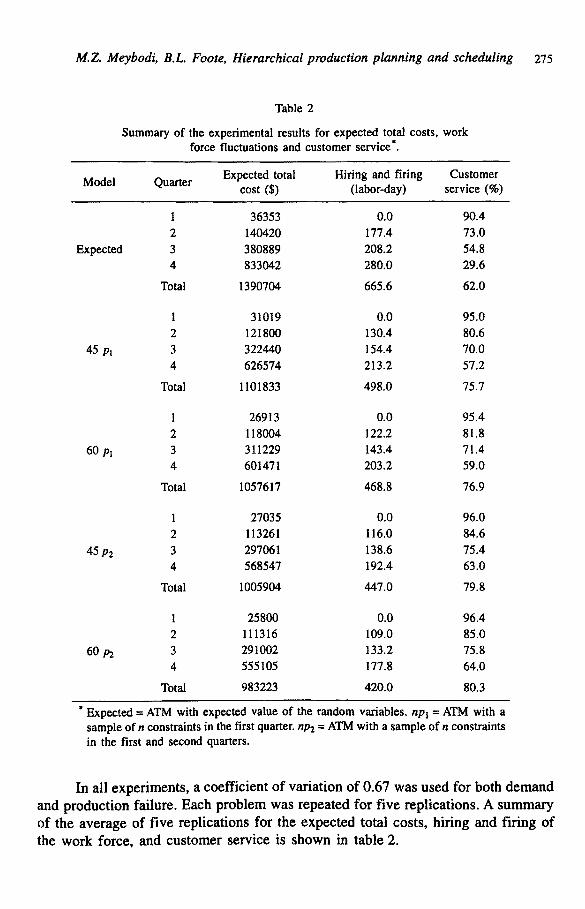
Table 2

Summary of the experimental results for expected total costs, work force fluctuations and customer service*.

Model Quarter Expected total Hiring and firing Customer cost ($) (labor-day) service (%)

1 36353 0.0 90.4 2 140420 177.4 73.0

Expected 3 380889 208.2 54.8 4 833042 280.0 29.6

Total 1390704 665.6 62.0

1 31019 0.0 95.0 2 121800 130.4 80.6

45 Pi 3 322440 154.4 70.0 4 626574 213.2 57.2

Total 1101833 498.0 75.7

1 26913 0.0 95.4 2 118004 122.2 81.8

60 Pl 3 311229 143.4 71.4 4 601471 203.2 59.0

Total 1057617 468.8 76.9

1 27035 0.0 96.0 2 113261 116.0 84.6

45 P2 3 297061 138.6 75.4 4 568547 192.4 63.0

Total 1005904 447.0 79.8

1 25800 0.0 96.4 2 111316 109.0 85.0

60 ,o2 3 291002 133.2 75.8 4 555105 177.8 64.0

Total 983223 420.0 80.3

* Expected = ATM with expected value of the random variables, npl = ATM with a sample of n constraints in the first quarter, np2 = ATM with a sample of n constraints in the first and second quarters.

In all exper iments , a coeff ic ient o f var ia t ion o f 0.67 was used for both d e m a n d

and produc t ion failure. Each p rob l em was repea ted fo r f ive repl icat ions. A s u m m a r y

o f the ave r age of f ive repl icat ions for the expec ted total costs , hir ing and f i r ing o f

the work force , and cus tomer service is shown in table 2.


From table 2, it is clear that SPWR with 45 sets of constraint samples outperforms the expected value approach. There is an improvement of 25% in the expected total costs, 25% in labor fluctuations, and a 22% improvement in customer service. Table 2 also shows that by modeling the first quarter with 60 constraint samples, there was an improvement of 4% in the expected total costs, 6% in labor fluctuations, and a 1.5% improvement in customer service over 45 constraint samples. The same small improvement is also true for the two-period stochastic modeling with sample sizes of 45 and 60 constraint sets. Table 2 also indicates that the expected total costs as well as labor fluctuations increase, and customer service declines from quarter 1 to quarter 4. This trend is due to initial inventory, a bottleneck at work centers 2 and 3, compounded forecast errors, and the fact that stochasticity in the last two quarters is not considered.

A set of statistical tests was applied to study the differences among the expected total costs, work force fluctuations, and customer service for each model. The test of hypotheses and the significant level from SAS output are summarized in table 3.

Table 3

Summary of the test of hypotheses.

Test no. H 0 HI H0 rejected?

1 #e - #45pl = 0 /'re - P45pl > 0 Yes (0.0004)*

2 0e - 045pl = 0 0e - 045pj > 0 Yes (0.0381)

3 ~,45pl - 2~ = 0 ~'4st, l - ~,e > 0 Yes (0.0002)

4 /z45pl -/Z6opl = 0 /Z4spl -/Z6Opl > 0 No (0.3710)

5 045pl - 06opl = 0 045pl - 06o~1 > 0 No (0.6460)

6 ~60pl - ~-4Spl = 0 A60pJ - ~45pt > 0 No (0.4677)

7 /.t45~l -/.t4sp2 = 0 /~4spl -/-t48,2 > 0 No (0.0514)

8 04spl - 045p2 = 0 04spl - 04sp: > 0 No (0.4210)

9 $48p2 - ~,4Spl = 0 245p 2 - 245,1 > 0 No (0.0756)

10 /.t6opl -/.t6op2 = 0 /Z6opl - g60~2 > 0 No (0.0792)

11 06o~1 - 060p2 = 0 060pl - 060p2 > 0 No (0.3962)

12 26Op2 - 2¢,op, = 0 ~ 2 - ~ot,, > 0 No (0.1086)

* (Signif icant level from SAS output.) /~ = expected total costs; 0 = work force f luctuation; :t = service level.

From table 3, the null hypothesis for the first three tests was rejected at the 0.05 significance level, which shows that the expected value approach was inferior in all criteria to the SPWR modeling. The null hypothesis for tests 4, 5, and 6 was not rejected at a significance level of 0.05, suggesting that the advantages gained by extending the number of samples from 45 to 60 in the first quarter is insignificant. Single period versus two-period stochastic models with 45 and 60 sample constraint


blocks were examined in tests 7 through 12. The null hypotheses for the expected total costs and customer service were not rejected at 0.05; however, they were rejected at the 0.10 significance level. This suggests that two-period stochastic modeling is better than single-period modeling. However, the number of samples in each period is not significant.

3.6. ANALYSIS OF VARIANCE (ANOVA)

A two-factor model was tested on each of the three criteria. The objective was to study if there is any interaction effect between the two factors of sample size and the number of stochastic periods. The factors were: 1 or 2 periods modeled stochastically and 45 or 60 constraint samples drawn from the constraint space. Tables 4, 5 and 6 show a summary of the ANOVA results for the three goals. In tables 4 - 6 , S Z is the sample size and N P is the number of periods.

Table 4

ANOVA results for total costs.

Source DF F value PR > F

SZ 1 1.36 0.2601 NP 1 9.27 0.0077 (SZ) (NP) 1 0.12 0.7355

Table 5

ANOVA results for hiring.


SZ 1 0.52 0.4824 NP 1 7.40 0.0152 (SZ) (NP) 1 0.00" 0.9960

*= truncated at two decimal points.

Table 4

ANOVA results for customer service.


SZ 1 0.51 0.4864 NP 1 7.40 0.0152 (SZ) (NP) 1 0.03 0.8749

From the above tables, there were no interaction effects between the two factors, and modeling two periods improved the expected total costs and the customer


service. Comparing this with the results of table 2, there is a marginal improvement in two-period modeling of about 5-8%. It is unlikely that extending the stochastic period beyond the two periods would give any significant improvement.

4. Conclusions

In this paper, a hierarchical production planning (HPP) and scheduling model was developed that integrates aggregate type decisions, family disaggregate decisions, lot-sizing and scheduling of the jobs. The model evaluates final production plans, updates the forecasts and proceeds on a rolling horizon basis. Random demand and production failure were explicitly incorporated into the aggregate type model. The incorporation of a simple heuristic scheduling algorithm is an important feature of the paper. The algorithm shows the actual progress of jobs through work centers and provides information regarding job tardiness, bottleneck work centers, and number of set-ups for each family. This information is useful for resolving production and capacity infeasibilities during the production process.

Incorporation of three criteria into the aggregate type problem is considered to be necessary for balancing the interests of the various decision-making functions in the organization. These criteria are: minimization of the total costs, minimization of the fluctuations in the level of work force, and maximization of the customer service. The aggregate problem is modeled as a goal program and solved using a sequential linear programming method.

A number of experiments were conducted to examine the performance of the HPP model. The primary objective of the experiments was to compare the performance of the constraint sample approximation method under different modeling complexities: (1) planning with 45 or 60 samples of constraint blocks in the aggregate type model; (2) one-period stochastic model or two-period stochastic model. Statistical t-tests and analysis of variance were used to study the differences among the different modeling procedures. The analysis of results indicated the following findings:

(I) The expected total cost associated with the expected value model is significantly greater than the expected total cost of the SPWR using the constraint sample approximation method. The main reason for the large difference is that the expected value approach basically neglects the distribution of the random variables and the magnitude of the competing costs.

(2) For the same reasons as in (1), the expected customer service for SPWR using the constraint sample approximation method is significantly greater than that obtained with the expected value model.

(3) The second objective of minimizing fluctuations in the level of work force is less sensitive to different policies than the other two objectives. The primary reason is mainly due to taking this objective directly from the aggregate goal program, while the other two objectives were computed after evaluation of the final disaggregate plans.


(4) Extending the number of samples of the stochastic constraints from 45 to 60 sets in the first quarter did not lead significantly (at the 0.05 level) to better production plans. This is mainly due to the normality assumption of the random variables, which suggests a set of 45 generated random vectors will likely estimate the complex possible scenarios in the future.

(5) The two-period stochastic model is significantly better than the single-period stochastic model, but there is no significant difference between the 45 or 60 sets of constraints.

(6) A large portion of the total costs is due to the bottleneck operations at work centers 2 and 3. Adding sufficient capacity to these work centers will greatly reduce the total costs and improve customer service.

References

[ 1 ] K.R. Baker, An experimental study of the effectiveness of rolling schedules in production planning, Dec. Sci. 8(1977)19-27.

[2] D. Bienstock and J.F. Shapiro, Optimizing resource acquisition decisions by stochastic programming, Manag. Sci. 34(1988)215-229.

[3] G.R. Bitran, E.A. Hans and A.C. Hax, Hierarchical production planning: A single stage system, Oper. Res. 29(1981)717-743.

[4] G.R. Bitran, E.A. Haas and A.C. Hax, Hierarchical production planning: A two stage system, Oper. Res. 30(1982)232-251.

[5] G.R. Bitran and A.C. Hax, On the design of hierarchical production planning systems, Dec. Sci. 8(1977)28-55.

[6] G.R. Bitran and H.H. Yanasse, Deterministic approximation to stochastic production problems, Oper. Res. 32(1984)999-1018.

[7] A.B. Borison, P.A. Morris and S.S. Oren, A state-of-the-world decomposition approach to dynamics and uncertainty in electric utility generation expansion planning, Oper. Res. 32(1984)1052-1068.

[8] M.R. Bowers and J.P. Jarvis, A hierarchical production planning and scheduling model, Dec. Sci. 23(1992)144-159.

[9] A. Chakranarty and G.E. Martin, Optimal multi-period inventory grouping for coordinated periodic replenishment under stochastic demand, Comp. Oper. Res. 15(1988)263-270.

[10] J. Ershler, G. Fontan and C. Mercer, Consistency of the disaggregation process in hierarchical planning, Oper. Res. 34(1986)464-469.

[11] B. Hansotia, Stochastic linear programming with recourse: A tutorial, Dec. Sci. 11(1980) 151-168.

[ 12] A.C. Hax and J.J. Golovin, Hierarchical production planning systems, in: Studies in Operations Management, ed. A.C. Hax (North-Holland, Amsterdam, 1978).

[13] A.C. Hax and H.C. Meal, Hierarchical integration of production planning and scheduling, in: Studies in Management Science, Logistics, ed. M.A. Geisler (North-Holland/American Elsevier, New York, 1975).

[14] R. Jagannathan, Linear programming with stochastic processes as parameters as applied to production planning, Ann. Oper. Res. 30(1991) 107-114.

[15] U.S. Karamarkar, Equalization of run out times, Oper. Res. 29(1981)757-762. [16] A.M. Law and W.D. Kelton, Simulation Modeling and Analysis, 2nd ed. (McGraw-Hill, 1991)

pp. 490-492. [17] G.K. Leong, M.D. Oliff and R.E. Markland, Improved hierarchical production planning, J. Oper.

Manag. 8(1989)90-114.


[18] J.J. Liberatore and T. Miller, A hierarchical production planning system, Interfaces 15(1985) 1-11.

[ 19] M.Z. Meybodi, Aggregate production planning and scheduling with multiple criteria and stochastic production events, Ph.D. Dissertation, School of Industrial Engineering, University of Oklahoma (1990), unpublished.

[20] E.M. Modiano, Derives demand and capacity planning under uncertainty, Oper. Res. 35(1987) 185-197.

[21] M.D. Oliff and E.E. Butch, Multiproduct production scheduling at Owen-Corning Fiberglass, Interfaces 15(1985)25-34.

[22] J.A. Orlicly, Material Requirement Planning (McGraw-Hill, New York, 1975). [23] D.T. Phillips, A. Ravindran and J. Solberg, Operations Research: Principles and Practice (Wiley,

1976). [24] G.H. Saad, Hierarchical production planning systems: Extensions and modifications, J. Oper.

Res. Soc. 41(1990)609-624. [25] L. Somlyody and R.J-B Wets, Stochastic optimization models for lake euthrophication management,

Oper. Res. 25(1988)660-681. [26] B. Strazicky, Some results concerning an algorithm for the discrete recourse problem, in: Stochastic

Programming, ed. M.A.H. Dempster (Academic Press, 1980). [27] U. Wemmerlov, The behavior of lot-sizing procedures in the presence of forecast errors, J. Oper.

Manag. 9(1989)37-47.

hierarchical production planning and scheduling with random demand and production failure

Documents