hierarchical production planning with demand constraints

Hierarchical production planning with demand constraintsq

Hong-Sen Yan*, Xiao-Dong Zhang, Min Jiang

Research Institute of Automation, Southeast University, Nanjing, Jiangsu 210096, China

Received 31 January 2003; revised 25 November 2003; accepted 7 January 2004

Abstract

This paper explores the hierarchical production planning (HPP) problem of flexible automated workshops

(FAWs), each of which has a number of flexible manufacturing systems (FMSs). The objective is to decompose

medium-term production plans (assigned to an FAW by ERP/MRP II) into short-term production plans (to be

executed by FMSs in the FAW) so as to minimize cost on the condition that demands have just been met. Herein,

the HPP problem is formulated by a linear programming model with the overload penalty different from the

underload penalty and with demand constraints. Since the scale of the model for a general workshop is too large to

be solved in the simplex method on a personal computer within acceptable time, Karmarkar’s algorithm and an

interaction/prediction algorithm, respectively, are used to solve the model, the former for the large scale problems

and the latter for the very large scale. With the help of the above-mentioned algorithms and HPP examples,

Karmarkar’s algorithm and the interaction/prediction algorithm are compared and analyzed, the results of which

show that the proposed approaches are quite effective and suitable for both ‘push’ and ‘pull’ production.

q 2004 Elsevier Ltd. All rights reserved.

Keywords: Flexible automated workshops; Flexible manufacturing systems; Hierarchical production planning; Karmarkar’s

algorithm; Interaction/prediction approach

1. Introduction

The problem of production planning for a flexible automated workshop (FAW) consisting of

flexible manufacturing systems (FMSs or cells) is important and worth studying. In a manufacturing

setting, production planning is essential to achieve efficient resource allocation over time in

meeting demands for finished products. Since the scope of PP problems generally prohibits a

monolithic modeling approach, a hierarchical production planning (HPP) approach has been widely

0360-8352/$ - see front matter q 2004 Elsevier Ltd. All rights reserved.

doi:10.1016/j.cie.2004.01.012

Computers & Industrial Engineering 46 (2004) 533–551www.elsevier.com/locate/dsw

q This manuscript was processed by Area Editor M. Dessouky.* Corresponding author. Tel.: þ86-25-8379-2418; fax: þ86-25-5771-2719.

E-mail address: [email protected] (H.-S. Yan).

http://www.elsevier.com/locate/dsw

advocated in the PP literature (Davis & Thompson, 1993). To model PP problems, the existing

hierarchical approaches usually employ the following concepts: (1) product disaggregation (Bitran,

Haas, & Hax, 1981; Bitran & Hax, 1977; Davis & Thompson, 1993; Graves, 1982; Hax & Meal,

1975; Newson, 1975; Saad, 1988; Simpson, 1999; Simpson & Erenguc, 1998; Yeh, Tarng, & Chen,

1988), (2) temporal decomposition (Karmarkar, 1988; Malakooti, 1989; Nguyen & Dupont, 1993;

Qiu & Burch, 1997; Tsubone, 1988), (3) process decomposition (Villa, 1989), and (4) event-

frequency decomposition (Akella, 1989; Gershwin, 1988; Kimemia & Gershwin, 1983). However,

those approaches are not quite suitable for the decomposition of medium-term production plans

(assigned to an FAW by ERP/MRP II short for enterprise resource planning/manufacturing resource

planning) into short-term production plans (to be executed by FMSs in the FAW). To be specific,

the product disaggregation only considers the structures of products instead of the organizational

structure of a manufacturing department. Although the process decomposition considers the

organizational structure of the manufacturing department, it only covers the manufacturing system

consisting of a forward chain of workshops. As the relationships among FMSs in an FAW are not

always serial or even very complicated, the process decomposition is inapplicable to the

decomposition of medium-term production plans for FAWs. And the temporal and event-frequency

decomposition do not consider the organizational structure of the manufacturing department as

such, either.

For this end, Yan (1997) and Yan and Jiang (1998) proposed two new approaches to the optimal

decomposition of production plans for FAWs with respect to delay interaction or not. By building up

linear quadratic models of PP problems and using interaction/prediction, their proposed approaches

optimally decompose medium-term production plans (assigned to an FAW by MRP II/CIMS short for

computer integrated manufacturing system) into short-term production plans (to be executed by FMSs in

the FAW) at a high speed. These approaches, combining the principles of both a temporal decomposition

and a process decomposition with the organizational structure of the FAW, are capable of solving very-

large-scale HPP problems. However, their overload and underload penalty are the same. In practice, the

wages for overtime are several times those for the usual hours and the underload only leads to the

decrease in the utilization of resources (such as men and equipment), so the overload penalty should be

much greater than the underload. Besides, only the manufacturers, that can agilely respond to and

completely satisfy users’ demands, can win a victory in the keen competition for markets, while the

overproduction will lead to the increase in finished-product inventory and production cost. No doubt, it is

desirable to just meet product demands without overproduction or underproduction. Thus, a linear

programming (LP) model with the overload penalty different from the underload penalty and with

demand constraints should be built up, for decomposing medium-term production plans (assigned to an

FAW by ERP/MRP II) into short-term production plans (to be executed by FMSs in the FAW). Because

the model for a general workshop is of thousands upon thousands of constraints and variables, it is

difficult to be solved by the simplex method on a personal computer within acceptable time. For this end,

we propose that Karmarkar’s algorithm and an interaction/prediction approach based on Karmarkar’s

algorithm, respectively, should be applied to solving the model, the former for the large scale problems

and the latter for the very large scale. The above-mentioned LP problem is also an HPP problem because

the Karmarkar’s algorithm and interaction/prediction approach based on Karmarkar’s algorithm for

solving it are in fact the methods to combine the principles of both a temporal decomposition and a

process one in HPP with the organizational structure of the FAW.

H.-S. Yan et al. / Computers & Industrial Engineering 46 (2004) 533–551534

2. Production planning model

An FAW under consideration in this paper is generalized from the flexible automated workshop of the

CIMS in the Chendu Aircraft Industry Company, which has two FMSs and two flexible direct numerical

control systems. To solve the general problem of HPP, we suppose that an FAW consists of a shop

computer, a material handling system (MHS), a tool handling system (THS), a shop testing and

monitoring system (STMS), and FMS12m. They are connected by a local area network (LAN), as shown

in Fig. 1. The shop computer manages the production of the FAW. Its main functions are: (1) receiving

medium-term production plans from ERP/MRP II and decomposing them into short-term production

plans (sent to the FMSs in the FAW); (2) from short-term production plans, developing tool requirement

plans (sent to the THS) and material requirement plans (sent to the MHS); and (3) reporting, in time, to

ERP/MRP II on error information, production situations and so on. Each of the FMSs in the FAW can

produce finished products or semi-finished products (which need sending to the successive FMSs for

further processing). The main functions of the FMSs are: (1) executing short-term production plans

coming from the shop computer, and (2) reporting to the shop computer on the error information and

production situations in time (Yan, Wang, Cui, & Zhang, 1997; Yan, Wang, Zhang, & Cui, 1998). The

layout of the FAW is shown in Fig. 2, in which the transfer of workpieces among FMSs and between

FMSs and the shop storage is described, with other details omitted.

The objective of HPP in the FAW is to obtain the lowest cost by simultaneously minimizing the

amount of in-process inventory, and the overload and underload on working centers over a finite horizon

of n time periods. Thus, the objective function of the HPP problem for the FAW can be described as

Fig. 1. Topologic structure of FAW’s LAN (Yan & Jiang, 1998).

Fig. 2. Layout of FAW (Yan & Jiang, 1998).

H.-S. Yan et al. / Computers & Industrial Engineering 46 (2004) 533–551 535

follows:

J ¼Xmi¼1

aTi xiðn þ 1Þ þ

Xn

k¼1

½aTi xiðkÞ þ bþT

i DþbiðkÞ þ b2Ti D2biðkÞ�

( )ð1Þ

where

m number of FMSs in an FAW.

n number of planning periods in a planning horizon H: H is generally a month or a week. A

planning period is shorter than H: A period is usually a week, a day or a shift.

mi number of working centers in FMSi:

ni number of types of workpieces which are manufactured by FMSi over H:

xiðkÞ in-process inventory of FMSi at the beginning of period k for k ¼ 1; 2;…; n þ 1: It is an ni

dimensional column vector.

DþbiðkÞ overload (or overtime) on working centers (NC machines, machining centers, etc.) of FMSi in

period k: It is an mi dimensional column vector.

D2biðkÞ underload (or idle time, undertime) on working centers of FMSi in period k: It is an mi


ai cost relative to an item of in-process inventory in FMSi: It is an ni dimensional column vector.

bþi cost coefficient related to overtime in FMSi: It is an mi dimensional column vector.

b2i cost coefficient related to idle resources (men, machines, etc.) in FMSi: It is an mi dimensional

column vector.

The FAW’s dynamic equation can be denoted by

xiðk þ 1Þ ¼ xiðkÞ2 uiðkÞ þ ziðkÞ þ GirðkÞ ð2aÞ

initial condition xið1Þ ¼ xi1 ð2bÞ

i ¼ 1; 2;…;m; k ¼ 1; 2;…; n

where

nf number of types of finished products which are processed by the FAW over H:

uiðkÞ workpieces (finished or semi-finished products) of planned production by FMSi in period k: It is

an ni dimensional column vector.

ziðkÞ number of semi-finished products which are sent from the other FMSs to FMSi in period k: It is

also known as interaction input and is an ni dimensional column vector.

rðkÞ input of blanks into the FAW in period k: It is an nf dimensional column vector. Each of its

components corresponds to products of a type.

Gi an ni £ nf Boolean matrix. It is an input matrix of FMSi:

Suppose that the time for transferring a workpiece between FMSs can be omitted. That is, as soon as a

semi-finished product has been processed by an FMS, it will be sent to another FMS. And it hardly takes


time to transfer the semi-finished product. Then the interaction equation can be represented by

ziðkÞ ¼Xmj¼1

LijujðkÞ ð3Þ

where

Lij an ni £ nj Boolean interaction matrix. It reflects the interaction between output of semi-finished

products from FMSj and input of semi-finished products into FMSi: The equation of a balance

between the load and the capacity of FMSi in period k is represented by

TiuiðkÞ2 DþbiðkÞ þ D2biðkÞ ¼ biðkÞ ð4Þ

where

Ti an mi £ ni matrix, the element at the jth row and the lth column of which represents the

processing time (it takes the jth working center in FMSi to process an item of workpieces of the

lth type).

biðkÞ processing time available to working centers of FMSi in period k: It is an mi dimensional column

vector.

The demand constraint of FMSi can be represented by

Xn

k¼1

CiuiðkÞ ¼ di ð5Þ

where

Ci an nf £ ni Boolean matrix. It is an output matrix of FMSi:

di demands for products out of FMSi over H: It is an nf dimensional column vector.

The output equations of products from the FAW can be described by

yðkÞ ¼Xmi¼1

yiðkÞ ð6Þ

yiðkÞ ¼ CiuiðkÞ ð7Þ

where

yðkÞ finished products of planned production by the FAW in period k: It is an nf dimensional column

vector whose jth ðj ¼ 1; 2;…; nÞ component is the yield of products of the jth type.

yiðkÞ finished products of planned production by FMSi in period k: It is a part of yðkÞ; and is also an nf



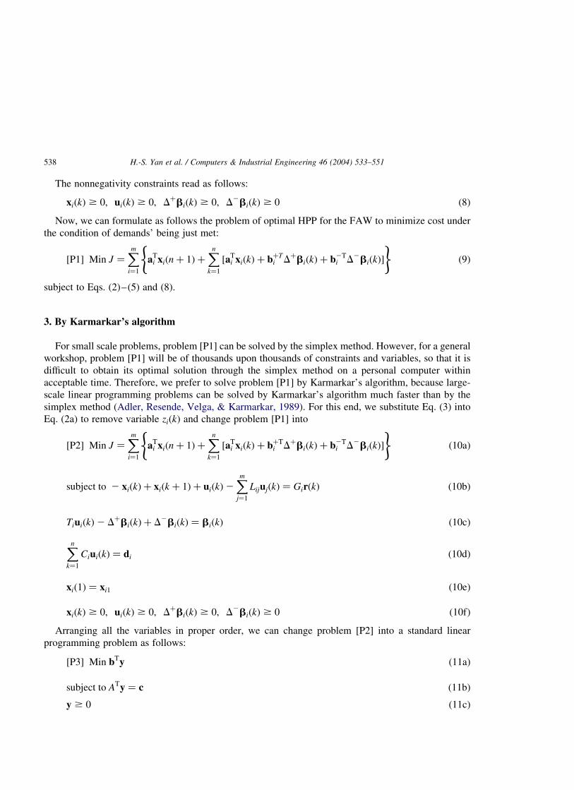
The nonnegativity constraints read as follows:

xiðkÞ $ 0; uiðkÞ $ 0; DþbiðkÞ $ 0; D2biðkÞ $ 0 ð8Þ

Now, we can formulate as follows the problem of optimal HPP for the FAW to minimize cost under

the condition of demands’ being just met:

½P1� Min J ¼Xmi¼1

aTi xiðn þ 1Þ þ

Xn

k¼1



( )ð9Þ

subject to Eqs. (2)–(5) and (8).

3. By Karmarkar’s algorithm

For small scale problems, problem [P1] can be solved by the simplex method. However, for a general

workshop, problem [P1] will be of thousands upon thousands of constraints and variables, so that it is

difficult to obtain its optimal solution through the simplex method on a personal computer within

acceptable time. Therefore, we prefer to solve problem [P1] by Karmarkar’s algorithm, because large-

scale linear programming problems can be solved by Karmarkar’s algorithm much faster than by the

simplex method (Adler, Resende, Velga, & Karmarkar, 1989). For this end, we substitute Eq. (3) into

Eq. (2a) to remove variable ziðkÞ and change problem [P1] into

½P2� Min J ¼Xmi¼1

aTi xiðn þ 1Þ þ

Xn

k¼1



( )ð10aÞ

subject to 2 xiðkÞ þ xiðk þ 1Þ þ uiðkÞ2Xmj¼1

LijujðkÞ ¼ GirðkÞ ð10bÞ

TiuiðkÞ2 DþbiðkÞ þ D2biðkÞ ¼ biðkÞ ð10cÞ

Xn

k¼1

CiuiðkÞ ¼ di ð10dÞ

xið1Þ ¼ xi1 ð10eÞ

xiðkÞ $ 0; uiðkÞ $ 0; DþbiðkÞ $ 0; D2biðkÞ $ 0 ð10fÞ

Arranging all the variables in proper order, we can change problem [P2] into a standard linear

programming problem as follows:

½P3� Min bTy ð11aÞ

subject to ATy ¼ c ð11bÞ

y $ 0 ð11cÞ


where A is a full rank m0 £ n0 matrix (where m0 $ n0), b and y are m0 dimensional column vectors, and c is

an n0 dimensional column vector.

Problem [P3] can be transformed into the corresponding dual linear programming problem and then

into a standard form suitable for being solved by Karmarkar’s algorithm I (Adler, Resende, Velga &

Karmarkar, 1989). Karmarkar’s algorithm provides an approach to the use of a nonlinear programming

method for solving linear programming problems by the implicit formulation of a logarithmic objective

function. Starting at an interior feasible solution x0; the algorithm generates a sequence of feasible

interior points {x1; x2;…; xk;…} with monotonically increasing objective values, terminating when a

stopping criterion is satisfied (Adler, Resende, Velga & Karmarkar, 1989). Thus, it is an interior point

method for linear programming. Since the algorithm requires that an initial interior feasible solution be

provided, a Phase I/Phase II scheme (Adler, Resende, Velga & Karmarkar, 1989) is used.

4. By interaction/prediction approach

The advantage of solving problem [P3] by Karmarkar’s algorithm is that the optimal solution can be

obtained. However, with the increase of FMSs, of working centers and of types of workpieces,

constraints and variables in problem [P3] will increase quickly, finally resulting in a failure to acquire the

optimal solution through Karmarkar’s algorithm on a personal computer within acceptable time. Thus,

the larger scale problems should be solved by the interaction/prediction approach based on Karmarkar’s

algorithm. Its basic ideas are: (1) by predicting interactions among FMSs, the FAW’s optimal HPP

problem [P1] is divided into m FMSs’ optimal PP sub-problems; (2) then solving each of the sub-

problems; and (3) improving the predictions and continuing the first two steps until the solution is

obtained. In the following, we shall go into details.

For any given z ¼ zp; problem [P1] can change into m FMSs’ optimal PP sub-problems. Thus, the

FMSi’s optimal PP sub-problem at the first level in the planning hierarchy becomes

½P4� Min Ji ¼ aTi xiðn þ 1Þ þ

Xn

k¼1


i DþbiðkÞ þ b2Ti D2biðkÞ� ð12aÞ

subject to 2 xiðkÞ þ xiðk þ 1Þ þ uiðkÞ ¼ zpi ðkÞ þ GirðkÞ ð12bÞ

TiuiðkÞ2 DþbiðkÞ þ D2biðkÞ ¼ biðkÞ ð12cÞ

Xn

k¼1

CiuiðkÞ ¼ di ð12dÞ

xið1Þ ¼ xi1 ð12eÞ

xiðkÞ $ 0; uiðkÞ $ 0; DþbiðkÞ $ 0; D2biðkÞ $ 0 ð12fÞ


Problem [P4] can be solved by Karmarkar’s algorithm in Section 3 to obtain uiðkÞ: Then zpi ðkÞ are

improved at the second level (coordination level) in the planning hierarchy by using

½zpi ðkÞ�lþ1 ¼

Xmj¼1

LijujðkÞ

24

35l

i ¼ 1; 2;…;m; k ¼ 1; 2;…; n ð13Þ

where l is the number of iterations.

From this, we can get the algorithm for solving the FAW’s optimal HPP problem [P1] as follows:

Algorithm 1. Interaction/prediction algorithm for FAW’s optimal HPP under the condition of demands’

being just met:

Step 1. At the coordination level, let l ¼ 1 and make conjectures upon initial values ziðkÞ ¼ zpi ðkÞ for

i ¼ 1; 2;…;m; k ¼ 1; 2;…; n: Then send them to the first level.

Step 2. Using Karmarkar’s algorithm, solve problem [P4] to obtain uiðkÞ ðk ¼ 1; 2;…; nÞ and xiðkÞ

ðk ¼ 2;…; n þ 1Þ; i ¼ 1; 2;…;m:

Step 3. Examine the norms kzpi ðkÞ2Pm

j¼1 LijujðkÞk2 in order to see whether they are all less than a very

little positive numeric. If they are, go to Step 5. Otherwise, go to Step 4.

Step 4. Using Eq. (13), update zpi ðkÞ: Let l ¼ l þ 1: Then go to Step 2.

Step 5. Stop iteration. Output short-term production plans upi ðkÞ to be executed by FMSi; finished pro-

ducts ypi ðkÞ of planned production by FMSi; in-process inventory xpi ðkÞ of FMSi and the lowest cost Jp:

By predicting interactions among FMSs, Algorithm 1 decomposes the FAW’s optimal HPP problem

into m FMS’s optimal PP sub-problems, reducing the complexity of the problem greatly and hence

speeding up the process of solving the problem. However, it cannot guarantee that the obtained solution

is optimal.

5. Computational experiments

Karmarkar’s algorithm in Section 3 and the interaction/prediction algorithm (Algorithm 1) in Section

4 have been implemented in VCþþ5.0. As A in Eq. (11b) is usually a large-scale sparse matrix, so only

nonzero elements of each column in A are stored by a single-chained-list structure in the implementation

of the two kinds of algorithms, to save the required storage space and to speed up the process of solving

the HPP problem. The search directions of Karmarkar’s algorithm can be computed by using the

improved Cholesky factorization method (an LU factorization method of symmetric positive definite

matrices) (Yuan, Zhang, Huang, & Wen, 1992) or by using the incomplete Cholesky factors as

preconditioners for a conjugate gradient method (for short, ICCG method) (Hu, 1991). The results

obtained after solving a number of HPP problems show that when the number of iterations of

Karmarkar’s algorithm is less than 12, the speed of computing search directions by the ICCG method is

faster than by the improved Cholesky factorization method, but when the number of iterations is greater

than 12, the speed by the former is usually slower or even far slower than by the latter. Thus, in the

implementation of the two kinds of algorithms, the ICCG method is adopted for the first 11 iterations and

the improved Cholesky factorization method adopted after the 11th iteration. In the following,


the application of, and the comparison between, the two kinds of algorithms are presented through

examples of HPP in FAWs.

In the following examples, the parameters of Karmarkar’s algorithm in Section 3 as well as

Karmarkar’s algorithm in Algorithm 1 are set as follows (Adler, Resende, Velga & Karmarkar, 1989). The

safety factor parameter is set tog ¼ 0:89 for the first 10 iterations andg ¼ 0:85 thereafter. Both algorithms

are terminated when the relative improvement in the objective function falls below 1 ¼ 1025: In phase I,

the value of the artificial variable cost defined in Eq. (4.7) (Adler, Resende, Velga & Karmarkar, 1989) is

determined by the constant m ¼ 105; the feasibility tolerance is set to 1f ¼ 0:01; and the condition xka , 0

satisfied by an interior feasible solution (Adler, Resende, Velga & Karmarkar, 1989) changes into xka , 10

ð10 ¼ 1026Þ: The diagonal update tolerance is set to d ¼ 0:1: In the implementation of the ICCG method,

the parameter v in the incomplete Cholesky factors is set to 0.6 and the termination tolerance of the

conjugate gradient algorithm is set to 1cg ¼ 10212 for the norm k·k1 (Hu, 1991).

The termination condition of Algorithm 1 is that each norm k·k2 in Step 3 is less than 0.1.

5.1. Push production

A push system produces finished or semi-finished products from the given production plan and the

given blanks input, i.e. pushing the production by the plan and the blanks input. Presented in the

following are 15 HPP examples (EX1 to EX15) for push production.

In Table 1, the results are obtained on a Pentium 2.4 GHz personal computer with 256 M memory

under Windows XP. The conditions of EX2 are the same as those of EX1 except that xi1 are zero vectors

and rðkÞ ¼ d=10 for k ¼ 1–10: The detailed conditions and results of EX1 are shown in Appendix A. On

average, Algorithm 1 is 56.49% faster than Karmarkar’s algorithm. But the optimal objective values for

Table 1

Comparative results of the two algorithms

Example FMS

number

Types of

part

Period

number

A in Eq. (11b) Karmarkar’s algorithm Algorithm 1

Row £ column Nonzero

elements

Running

time(s)

J* Running

time(s)

J*

EX1 5 6 10 700 £ 356 1502 3.391 554.600000 2.343 554.600000

EX2 5 6 10 700 £ 356 1502 3.391 216.950000 2.360 216.950000

EX3 6 20 10 2600 £ 1320 8342 83.360 370.900000 35.281 371.365648

EX4 8 30 10 2800 £ 1430 7211 61.500 87.993783 21.765 88.129604

EX5 4 4 40 2560 £ 1284 5544 179.828 46.300000 177.109 46.325144

EX6 4 6 40 2080 £ 1046 4745 65.390 38.000000 60.671 38.000000

EX7 4 6 40 2320 £ 1166 5223 88.891 39.500000 87.218 39.502345

EX8 4 6 40 2960 £ 1486 6859 199.563 53.600000 189.703 53.628352

EX9 5 6 40 2800 £ 1406 6062 142.062 867.800000 89.235 867.800000

EX10 4 6 40 2560 £ 1286 5702 108.047 330.400000 116.421 330.400000

EX11 5 7 40 3680 £ 1847 8457 375.438 98.200000 267.093 98.214338

EX12 4 10 40 4320 £ 2170 11,006 402.500 240.800000 355.828 240.804413

EX13 6 20 40 10,400 £ 5220 33,632 7923.781 1483.600000 3178.890 1483.695773

EX14 8 30 40 11,200 £ 5630 29,141 2863.016 352.000000 1349.109 352.002778


Algorithm 1 are, on the average, 0.03% greater than those for Karmarkar’s algorithm. Although

the numbers of part types and FMSs, and the size of matrix A; of EX4 (or alternatively EX14) are greater

than those of EX3 (or alternatively EX13), the total number of nonzero elements of the former is less

than that of the latter. This is because the total number of working centers used in all sequences of all part

types of EX4 (or alternatively EX14) is 156 less than that of EX3 (or alternatively EX13) so that in each

period the total nonzero elements in all matrixes Ti ði ¼ 1; 2;…; 8Þ of the former are 156 less than those

in all matrixes Ti ði ¼ 1; 2;…; 6Þ of the latter and in 10 (or alternatively 40) periods the total nonzero

elements of the former are 1560 (or alternatively 6240) less than those of the latter. Although the number

of part types (or alternatively FMSs) of EX6 (or alternatively EX9) is greater than that of EX5 (or

alternatively EX8), the size of matrix A of the former is smaller than that of the latter. This is becausePi ðni þ miÞ for EX6 (or alternatively EX9) is less than that for EX5 (or alternatively EX8). When the

conditions are the same as those in EX14 except for 50 planning periods in a planning horizon H;A in

Eq. (11b) becomes a full rank 14,000 £ 7030 matrix and has 36,451 nonzero elements, which is known

as EX15. However, we cannot run our software of Karmarkar’s algorithm for EX15 on a Pentium

2.4 GHz personal computer with 256 M memory under Windows XP because of insufficient virtual

memory, while we obtain the optimal solution with Jp ¼ 441:016893 after having run our software of

Algorithm 1 on EX15 under the same condition for 2632.969 s.

Problems [P2] and [P4] and examples EX1 to EX15 are for the case that rðkÞ is given, i.e. for ‘push’

production. If GirðkÞ in Eq. (10b) is moved to the left of Eq. (10b) and rðkÞ $ 0 is added to Eq. (10f),

then the optimal rpðkÞ can also be obtained by solving problem [P2], i.e. for ‘pull’ production.

5.2. Pull production

A pull system generates the blank requirements and produces finished or semi-finished products from

the given product demand plan, that is, pulling the production by demands. The following is an HPP

example for a pull system.

The conditions are the same as those in EX1 in ‘push’ production except that rðkÞ is not given

beforehand.

For Karmarkar’s algorithm, A in Eq. (11b) becomes a full rank 760 £ 356 matrix and has 1562

nonzero elements, which is different from EX1 in ‘push’ production because of the movement of GirðkÞin Eq. (10b) to the left of Eq. (10b). Having run our software of Karmarkar’s algorithm for 4.625 s on a

Pentium 2.4 GHz personal computer with 256M memory under Windows XP, we obtain the optimal

solution including Jp; upi ðkÞ; ypi ðkÞ; xp

i ðkÞ and rpðkÞ: The optimal objective value Jp is equal to

537.496481, which is 3.08% lower than that by Karmarkar’s algorithm in EX1 in ‘push’ production.

Having rounded rpðkÞ by

RpðkÞ ¼ round rpðkÞ þXk21

t¼1

ðrpðtÞ2 RpðtÞÞ

!ð14Þ

we get

Rpð1Þ ¼ ð0 2 4 10 0 4ÞT

RpðkÞ ¼ ð8 9 5 9 7 12ÞT for k ¼ 2–10


6. Conclusions

In this paper, we have addressed the HPP problem of flexible automated workshops. First of all, the

HPP problem is formulated by a linear programming model with the overload penalty different from the

underload penalty and with demand constraints. The objective is to decompose medium-term production

plans into short-term production plans and minimize cost under the condition of demands’ being just

satisfied. Because the scale of the model for a general workshop is too large to be solved by the simplex

method on a personal computer within acceptable time, Karmarkar’s algorithm and Algorithm 1 are

adopted for solving the model. With the help of the above-mentioned algorithms, some typical examples

of HPP have been studied, with the results showing that

(1) Karmarkar’s algorithm can guarantee the optimal solutions to HPP problems, but Algorithm 1

cannot;

(2) Algorithm 1 is on an average 56.49% faster than Karmarkar’s algorithm, but the optimal objective

values for Algorithm 1 are on an average 0.03% greater than those for Karmarkar’s algorithm;

(3) Karmarkar’s algorithm is suitable for solving large-scale problems, and Algorithm 1 for very-large-

scale ones;

(4) The proposed approaches are quite effective in that the optimal solutions of the very large scale HPP

problems with eight FMSs, 30 types of parts totalling 1960 and 50 planning periods in a planning

horizon H can be obtained by Algorithm 1 within 2632.969 s on a Pentium 2.4 GHz personal

computer with 256 M memory;

(5) The proposed approaches are very suitable for decomposing medium-term production plans into

short-term production plans so as to obtain the lowest cost under the condition of demands’ being

just satisfied.

The HPP problem [P3] and Step 2 in Algorithm 1 can also be solved by other interior point

methods for linear programming (Megiddo, Mizuno, & Tsuchiya, 1998; Renegar, 1988; Sturm &

Zhang, 1998) instead of by Karmarkar’s algorithm. However, since those methods have not been

demonstrated through a convincing number of computational experiments, we employ Karmarkar’s

algorithm to solve the HPP problems herein.

Problems [P2] and [P4] are for the case that rðkÞ is given, that is, for ‘push’ production. If

GirðkÞ in Eq. (10b) is moved to the left of Eq. (10b) and GirðkÞ in Eq. (12b) moved to the left of

Eq. (12b) and if rðkÞ $ 0 is added to Eqs. (10f) and (12f), then the optimal rpðkÞ can also be

obtained by solving problems [P2] and [P4], that is, for ‘pull’ production. And the optimal

objective values for ‘pull’ production are less than those for ‘push’ production under the same

conditions.

Only the number of workpieces of planned production by each FMS in each period is determined

through Karmarkar’s algorithm and Algorithm 1. To develop the real production plan to be executed

by each FMS in each period, we must add such parameters as part no, part priority, available

machine (or working center), NC program, processing time and tool to the number (Yan, Wang, Cui

& Zhang, 1997; Yan, Wang, Zhang & Cui, 1998).


Acknowledgements

This research was supported by the National Natural Science Foundation of China under grant

60443001 and by the National High Tech R&D Program of China under grant 863-511-943-005. We

thank Area Editor M. Dessouky, the anonymous referees and Professor Li Lu for valuable comments and

suggestions.

Appendix A. A detailed example

Without loss of generality, suppose that an FAW consists of five FMSs whose functions are

complementary. Each FMS is composed of several working centers whose functions are alike and/or

complementary. The week production plan (assigned to the FAW by ERP/MRP II) is shown in Table A1.

From Table A1, we know that there are six types of parts whose processing routes are flexible and are of

the property of job shop. Parts are sent to one of the available working centers for each sequence. It is a

5-day week. A workday is divided into two shifts. Times (excluding machine repairing times, etc.)

available to working centers each shift are shown in Table A2.

From Table A1 and Eq. (4), we obtain (Yan & Jiang, 1998):

T1 ¼

0:300 0 0:540 0:360

0:300 0 1:000 0:255

1:000 0:420 0:900 0:255

2664

3775 T2 ¼

0:630 0:225 0 0:330

0:780 0:780 0:450 0:810

0:540 0:225 0:400 0

1:200 0 0:400 0

26666664

37777775

T3 ¼

0:600 0:600 0:400

0:570 0:360 0

0:840 0:360 0

0:600 0 0:400

26666664

37777775 T4 ¼

0:900 0:560 0:285

1:300 0 0:285

0:600 0 0:420

2664

3775

T5 ¼

1:420 0:270 0 0

0:810 0 0:740 0:540

0 0:270 0:960 1:100

2664

3775

From Table A1 and Eqs. (2), (3) and (5), we get:

G1 ¼

0 1 0 0 0 0

0 0 1 0 0 0

0 0 0 0 0 0

0 0 0 0 1 0

26666664

37777775 ¼

ð1; 2Þ ¼ 1

ð2; 3Þ ¼ 1

ð4; 5Þ ¼ 1

ðotherÞ ¼ 0

26666664

37777775

4£6


Table A1

Week production plan

Part Sequence FMS Available working

centers

Lot Processing

time (h)

P1 5 3 WC31, WC34 80 1.20

10 WC32 0.57

15 WC33 0.84

20 4 WC42 1.30

25 WC41 0.90

30 WC43 0.60

35 2 WC22 0.78

40 WC23 0.54

45 WC21 0.63

50 WC24 1.20

P2 5 1 WC11, WC12 90 0.60

10 WC13 1.00

15 5 WC51 1.42

20 WC52 0.81

25 4 WC41 0.56

P3 5 1 WC13 60 0.42

10 2 WC21, WC23 0.45

15 WC22 0.78

20 5 WC51, WC53 0.54

P4 5 3 WC32, WC33 100 0.72

10 WC31 0.60

15 2 WC22 0.45

20 WC23, WC24 0.80

25 1 WC11 0.54

30 WC12 1.00

35 WC13 0.90

P5 5 1 WC11 70 0.36

10 WC12, WC13 0.51

15 5 WC52 0.74

20 WC53 0.96

25 4 WC41, WC42 0.57

30 WC43 0.42

P6 5 2 WC21 120 0.33

10 WC22 0.81

15 5 WC52 0.54

20 WC53 1.10

25 3 WC31, WC34 0.80


G2 ¼ð4; 6Þ ¼ 1

ðotherÞ ¼ 0

" #4£6

G3 ¼

ð1; 1Þ ¼ 1

ð2; 4Þ ¼ 1

ðotherÞ ¼ 0

2664

3775

3£6

G4 ¼ ½ðotherÞ ¼ 0�3£6 ¼ ½0�3£6 G5 ¼ ½0�4£6

L12 ¼ð3; 3Þ ¼ 1

ðotherÞ ¼ 0

" #4£4

L21 ¼ð2; 2Þ ¼ 1

ðotherÞ ¼ 0

" #4£4

L23 ¼ð3; 2Þ ¼ 1

ðotherÞ ¼ 0

" #4£3

L24 ¼ð1; 1Þ ¼ 1

ðotherÞ ¼ 0

" #4£3

L35 ¼ð3; 4Þ ¼ 1

ðotherÞ ¼ 0

" #3£4

L43 ¼ð1; 1Þ ¼ 1

ðotherÞ ¼ 0

" #3£3

L45 ¼

ð2; 1Þ ¼ 1

ð3; 3Þ ¼ 1

ðotherÞ ¼ 0

2664

3775

3£4

L51 ¼

ð1; 1Þ ¼ 1

ð3; 4Þ ¼ 1

ðotherÞ ¼ 0

2664

3775

4£4

L52 ¼

ð2; 2Þ ¼ 1

ð4; 4Þ ¼ 1

ðotherÞ ¼ 0

2664

3775

4£4

L11 ¼ L15 ¼ L22 ¼ L25 ¼ L55 ¼ ½0�4£4

L13 ¼ L14 ¼ L53 ¼ L54 ¼ ½0�4£3 L31 ¼ L32 ¼ L41 ¼ L43 ¼ ½0�3£4

L33 ¼ L34 ¼ L44 ¼ ½0�3£3 C1 ¼ð4; 3Þ ¼ 1

ðotherÞ ¼ 0

" #6£4

C2 ¼ð1; 1Þ ¼ 1

ðotherÞ ¼ 0

" #6£4

C3 ¼ð6; 3Þ ¼ 1

ðotherÞ ¼ 0

" #6£3

Table A2

Times available to working centers each shift

FMS Working center (unit: h)

1 2 3 4

1 14 21 28

2 14 28 14 21

3 21 7 14 7

4 14 14 7

5 14 14 21


C4 ¼

ð2; 2Þ ¼ 1

ð5; 3Þ ¼ 1

ðotherÞ ¼ 0

2664

3775

6£3

C5 ¼ð3; 2Þ ¼ 1

ðotherÞ ¼ 0

" #6£4

From Table A2 and Eq. (4), we have

b1ðkÞ ¼ ð14 21 28ÞT b2ðkÞ ¼ ð14 28 14 21ÞT

b3ðkÞ ¼ ð21 7 14 7ÞT b4ðkÞ ¼ ð14 14 7ÞT

b5ðkÞ ¼ ð14 14 21ÞT

for k ¼ 1; 2;…; 10:

From Table A1 and Eq. (5), we get

d1 ¼ ð0 0 0 100 0 0ÞT d2 ¼ ð80 0 0 0 0 0ÞT

d3 ¼ ð0 0 0 0 0 120ÞT d4 ¼ ð0 90 0 0 70 0ÞT

d5 ¼ ð0 0 60 0 0 0ÞT

d ¼X5

i¼1

di ¼ ð80 90 60 100 70 120ÞT

Let input of blanks into the FAW

rð1Þ ¼ ð0 0 0 1 0 3ÞT rð2Þ ¼ ð7 9 3 10 5 12ÞT

rðkÞ ¼ ð8 9 6 10 7 12ÞT for k ¼ 3–10

Let initial in-process inventory

x11 ¼ x21 ¼ x51 ¼ ð3 3 3 3ÞT x31 ¼ x41 ¼ ð3 3 3ÞT

Let coefficients in Eq. (1)

a1 ¼ ð2:500 2:500 8:925 2:500ÞT a2 ¼ ð16:025 3:550 5:800 2:500ÞT


a3 ¼ ð2:500 2:500 9:450ÞT a4 ¼ ð9:025 12:075 8:925ÞT

bþ1 ¼ bþ

4 ¼ bþ5 ¼ ð1 1 1 ÞT bþ

2 ¼ bþ3 ¼ ð1 1 1 1ÞT

b21 ¼ b2

4 ¼ b25 ¼ ð0:25 0:25 0:25ÞT b2

2 ¼ b23 ¼ ð0:25 0:25 0:25 0:25ÞT

For Karmarkar’s algorithm, A in Eq. (11b) becomes a full rank 700 £ 356 matrix and has 1502

nonzero elements. Having run our software of Karmarkar’s algorithm for 3.391 s on a Pentium 2.4 GHz

personal computer with 256 M memory under Windows XP, we obtain FMSs’ optimal shift production

plans, as shown in Tables A3–A7. For simplicity, each plan only shows the number of workpieces

(finished or semi-finished products) of planned production by the corresponding FMS every shift, that is,

upi ðkÞ for i ¼ 1; 2;…; 5; k ¼ 1; 2;…; 10:

From Tables A3–A7, we know thatP10

k¼1 ypi ðkÞ ¼P10

k¼1 Ciupi ðkÞ ¼ di for i ¼ 1; 2;…; 5: In the real

production situations, the numbers of workpieces of planned production by FMSs are usually integers.

Thus, unless all components of upi ðkÞ are integers, up

i ðkÞ can be rounded by

Upi ðkÞ ¼ round up

i ðkÞ þXk21

t¼1

ðupi ðtÞ2 Up

i ðtÞÞ

!ð15Þ

where Upi ðkÞ are integer vectors of workpieces of planned production by FMSi.

Table A3

FMS1’s shift production plans

Part Period

1 2 3 4 5 6 7 8 9 10

P2 3 9 9 9 9 9 9 9 9 9

P3 3 3 6 6 6 6 6 6 6 6

P4 10 10 10 10 10 10 10 10 10 10

P5 3 5 7 7 7 7 7 7 7 7

Table A4


Part Period

1 2 3 4 5 6 7 8 9 10

P1 9 7 8 8 8 8 8 8 8 8

P3 6 3 6 6 6 6 6 6 6 6

P4 7 10 10 10 10 10 10 10 10 10

P6 6 12 12 12 12 12 12 12 12 12


Besides, the optimal objective value Jp is 554.60. The number of iteration is 22. The in-process

inventories xpi ðkÞ read as follows:

xp1ðkÞ ¼ xp2ðkÞ ¼ xp

5ðkÞ ¼ ð0 0 0 0ÞT

xp3ðkÞ ¼ xp4ðkÞ ¼ ð0 0 0ÞT

for k ¼ 2; 3;…; 11:

Then, we make conjectures upon initial values

zp1ðkÞ ¼ zp2ðkÞ ¼ zp5ðkÞ ¼ ð20 20 20 20ÞT

zp3ðkÞ ¼ zp4ðkÞ ¼ ð20 20 20ÞT

for k ¼ 1; 2;…; 10:

Table A6


Part Period

1 2 3 4 5 6 7 8 9 10

P1 6 7 8 8 8 8 8 8 8 8

P2 9 9 9 9 9 9 9 9 9 9

P5 9 5 7 7 7 7 7 7 7 7

Table A7


Part Period

1 2 3 4 5 6 7 8 9 10

P2 6 9 9 9 9 9 9 9 9 9

P3 9 3 6 6 6 6 6 6 6 6

P5 6 5 7 7 7 7 7 7 7 7

P6 9 12 12 12 12 12 12 12 12 12

Table A5


Part Period

1 2 3 4 5 6 7 8 9 10

P1 3 7 8 8 8 8 8 8 8 8

P4 4 10 10 10 10 10 10 10 10 10

P6 12 12 12 12 12 12 12 12 12 12


Next, having run our software of Algorithm 1 on Example 1 under the same condition for 2.343 s, we

obtain the same Jp; upi ðkÞ; yp

i ðkÞ and xpi ðkÞ as those by Karmarkar’s algorithm. In this case, Algorithm 1 is

44.73% faster than Karmarkar’s algorithm.

References

Adler, I., Resende, M. G. C., Velga, G., & Karmarkar, N. (1989). An implementation of Karmarkar’s algorithm for linear

programming. Mathematical Programming, 44(3), 297–335.

Akella, R. (1989). Real time part dispatch in flexible assembly test and manufacturing systems. Operations research models in

flexible manufacturing systems, Wien: Springer, pp. 1–73.

Bitran, G. R., Haas, E. A., & Hax, A. C. (1981). Hierarchical production planning: A single state system. Operations Research,

29(4), 717–743.

Bitran, G. R., & Hax, A. C. (1977). On the design of hierarchical production planning systems. Decision Sciences, 8, 28–55.

Davis, W. J., & Thompson, S. D. (1993). Production planning and control hierarchy using a generic controller. IIE

Transactions, 25(4), 26–45.

Gershwin, S. B. (1988). A hierarchical framework for discrete event scheduling in manufacturing systems. Proceedings of

IIASA Conference on Discrete Event System: Models and Applications (Sopron, Hungary, 1987), Berlin: Springer,

pp. 197–216.

Graves, S. C. (1982). Using Lagrangian techniques to solve hierarchical production planning problems. Management Science,

28(3), 260–275.

Hax, A. C., & Meal, H. C. (1975). Hierarchical integration of production planning and scheduling. In M. A. Geisler (Ed.),

Studies in management sciences: Vol. I, logistics. New York: Elsevier, pp. 53–69.

Hu, J. G. (1991). Iterative solution of systems of linear algebraic equations. Beijing: Science Press, (in Chinese).

Karmarkar, U. S. (1988). A hierarchical scheduling system for the CIM environment. The Collection of Refereed Papers

Presented at the Ninth International Conference on Production Research (Cincinnati, Ohio, 1987), Amsterdam: Elsevier,

pp. 271–277.

Kimemia, J., & Gershwin, S. B. (1983). An algorithm for the computer control of a flexible manufacturing system. IIE

Transactions, 15(4), 353–362.

Malakooti, B. (1989). A gradient-based approach for solving hierarchical multi-criteria production planning problems.

Computers and Industrial Engineering, 16(3), 407–417.

Megiddo, N., Mizuno, S., & Tsuchiya, T. (1998). A modified layered-step interior-point algorithm for linear programming.

Mathematical Programming, 82(3), 339–355.

Newson, E. F. P. (1975). Multi-item lot size scheduling by heuristic, Part I: with fixed resources, Part II: with variable resources.

Management Science, 21(10), 1186–1203.

Nguyen, P. L., & Dupont, L. (1993). Production management of a steel manufacturing system: a hierarchical planning model.

Computers and Industrial Engineering, 25(1–4), 81–84.

Qiu, M. M., & Burch, E. E. (1997). Hierarchical production planning and scheduling in a multi-product, multi-machine

environment. International Journal of Production Research, 35(11), 3023–3042.

Renegar, J. (1988). A polynomial-time algorithm, based on Newton’s method, for linear programming. Mathematical

Programming, 40(1), 59–93.

Saad, G. H. (1988). An optimization approach for the disaggregation of aggregate production plans. Proceedings of the Second

International Conference on Expert Systems and the Leading Edge in Production Planning and Control (Charleston, SC,

1988), New York: North-Holland, pp. 305–318.

Simpson, N. C. (1999). Multiple level production planning in rolling horizon assembly environments. European Journal of

Operational Research, 114(1), 15–28.

Simpson, N. C., & Erenguc, S. S. (1998). Improved heuristic methods for multiple stage production planning. Computers and

Operations Research, 25(7/8), 611–623.

Sturm, J. F., & Zhang, S. (1998). An interior point method, based on rank-1 updates, for linear programming. Mathematical

Programming, 81(1), 77–87.


Tsubone, H. (1988). An analytical model for hierarchical production planning. The Collection of Refereed Papers Presented at

the Ninth International Conference on Production Research (Cincinnati, Ohio, 1987), Amsterdam: Elsevier, pp. 216–222.

Villa, A. (1989). Hierarchical architectures for production planning and control. Operations Research Models in Flexible

Manufacturing Systems, Wien: Springer, pp. 261–288.

Yan, H. S. (1997). An interaction/prediction approach to hierarchical production planning and control with delay interaction

equations. Computer Integrated Manufacturing Systems, 10(4), 309–320.

Yan, H. S., & Jiang, Z. J. (1998). An interaction/prediction approach to solving problems of hierarchical production planning in

flexible automation workshops. International Journal of Computer Integrated Manufacturing, 11(6), 513–523.

Yan, H. S., Wang, N. S., Cui, X. Y., & Zhang, J. G. (1997). Modeling, scheduling and control of flexible manufacturing systems

by extended high-level evaluation Petri nets. IIE Transactions, 29(2), 147–158.

Yan, H. S., Wang, N. S., Zhang, J. G., & Cui, X. Y. (1998). Modelling, scheduling and simulation of flexible manufacturing

systems using extended stochastic high-level evaluation Petri nets. Robotics and Computer-Integrated Manufacturing,

14(2), 121–140.

Yeh, H. M., Tarng, M. Y., & Chen, W. C. (1988). An iterative algorithm to solve hierarchical production planning problems.

The Collection of Refereed Papers Presented at the 9th International Conference on Production Research (Cincinnati,

Ohio, 1987), Amsterdam: Elsevier, pp. 209–215.

Yuan, W. P., Zhang, L. M., Huang, X. Q., & Wen, Z. C. (1992). Numerical Analysis. Nanjing, Jiangsu: Southeast University

Press (in Chinese).


hierarchical production planning with demand constraints

Documents