PSYCHOMETRIKA—VOL. 75, NO. 1, 33–57MARCH 2010DOI: 10.1007/S11336-009-9136-X

HIGH-DIMENSIONAL EXPLORATORY ITEM FACTOR ANALYSISBY A METROPOLIS–HASTINGS ROBBINS–MONRO ALGORITHM

LI CAI

UNIVERSITY OF CALIFORNIA, LOS ANGELES

A Metropolis–Hastings Robbins–Monro (MH-RM) algorithm for high-dimensional maximum mar-ginal likelihood exploratory item factor analysis is proposed. The sequence of estimates from the MH-RMalgorithm converges with probability one to the maximum likelihood solution. Details on the computerimplementation of this algorithm are provided. The accuracy of the proposed algorithm is demonstratedwith simulations. As an illustration, the proposed algorithm is applied to explore the factor structure un-derlying a new quality of life scale for children. It is shown that when the dimensionality is high, MH-RMhas advantages over existing methods such as numerical quadrature based EM algorithm. Extensions ofthe algorithm to other modeling frameworks are discussed.

Key words: stochastic approximation, SA, item response theory, IRT, Markov chain Monte Carlo,MCMC, numerical integration, categorical factor analysis, latent variable modeling, structural equationmodeling.

1. Introduction

Full-information Item Factor Analysis (IFA; Bock, Gibbons, & Muraki, 1988) has long beena useful tool for exploring the latent structure underlying educational and psychological tests. Itis also being increasing utilized in mental health and quality of life research due to a recent surgeof interest among researchers in the application of item response theory to develop standardizedmeasurement instruments for patient reported outcomes. A notable example is the National Insti-tutes of Health Patient Reported Outcomes Measurement Information System (PROMIS; Reeve,Hays, Bjorner, Cook, Crane, & Teresi, 2007). IFA proves to be crucial in these new domains ofapplication, yet despite recent advances in methods for fitting high-dimensional item responsetheory models, maximum marginal likelihood estimation in IFA remains a difficult numericalproblem. The biggest obstacle stems from the need to evaluate intractable high-dimensional in-tegrals in the likelihood function for the item parameters. Depending on how the integrals areapproximated, existing algorithms for maximum likelihood estimation in IFA can be groupedroughly into the following four classes.

The first class involves adaptive Gaussian quadrature. By replacing fixed-point quadraturerules with adaptive rules (Liu & Pierce, 1994; Naylor & Smith, 1982), approximations to thehigh-dimensional integrals impose significantly less computational burden. Adapting the quadra-ture nodes also stabilizes likelihood computations, because when the number of items is large

I thank the editor, the AE, and the reviewers for helpful suggestions. I am indebted to Drs. Chuanshu Ji, Robert Mac-Callum, and Zhengyuan Zhu for helpful discussions. I would also like to thank Drs. Mike Edwards and David Thissenfor supplying the data sets used in the numerical demonstrations. The author gratefully acknowledges financial supportfrom Educational Testing Service (the Gulliksen Psychometric Research Fellowship program), National Science Foun-dation (SES-0717941), National Center for Research on Evaluation, Standards and Student Testing (CRESST) throughaward R305A050004 from the US Department of Education’s Institute of Education Sciences (IES), and a predoctoraladvanced quantitative methods training grant awarded to the UCLA Departments of Education and Psychology fromIES. The views expressed in this paper are of the author’s alone and do not reflect the views or policies of the fundingagencies.

Requests for reprints should be sent to Li Cai, GSE & IS, UCLA, Los Angeles, CA, USA 90095-1521. E-mail:lcai@ucla.edu

© 2009 The Psychometric Society. This article is published with open access at Springerlink.com33

34 PSYCHOMETRIKA

the likelihood becomes so concentrated that standard Gaussian quadrature formulae do not ac-curately capture its mass. With care in implementation, pointwise convergence of the estimatesto a local maximum of the likelihood function can be obtained (e.g., Rabe-Hesketh, Skrondal,& Pickles, 2005; Schilling & Bock, 2005). Because of over two decades of success with Bockand Aitkin’s (1981) EM algorithm, adaptive quadrature based EM algorithm is often considereda gold standard against which other algorithms are compared. It is also possible to use adaptivequadrature in a Newton–Raphson algorithm such as in GLLAMM (Rabe-Hesketh, Skrondal, &Pickles, 2004a). Despite its popularity, adaptive quadrature still limits the number of factors thatan IFA software can handle simply because the number of quadrature points must grow expo-nentially as the dimensionality of the latent traits increases. This phenomenon is often referredto as the “curse of dimensionality” in the literature. In addition, if the EM algorithm is usedin conjunction with quadrature, variability information of parameter estimates is not an auto-matic by-product. Additional computation for parameter standard errors is required (see, e.g.,Cai, 2008b) upon EM’s convergence. As a result, TESTFACT does not print standard errors inits output.

The second class is characterized by the use of Laplace approximation (Tierney & Kadane,1986). Applications of this method can be found in Kass and Steffey (1989), Thomas (1993), andHuber, Ronchetti, and Victoria-Feser (2004). In the context of IFA, the Laplace method is essen-tially adaptive Gauss–Hermite integration with 1 quadrature point. It is computationally fast (see,e.g., Raudenbush, Yang, & Yosef, 2000, in a slightly different application), but a notable featureof this method is that the error of approximation decreases only as the number of items increases.When few items are administered to each examinee, such as in an adaptive test design, or whenthere are relatively few items loading on a factor, such as in the presence of testlets (Wainer &Kiely, 1987), the degree of imprecision in approximation can become substantial and may leadto biased parameter estimates (Joe, 2008). Raudenbush et al. (2000) argue for the use of higher-order Laplace approximation, but the complexity of software implementation grows dramaticallyas the order of approximation increases. In addition, the truncation point in the asymptotic seriesexpansion (6th degree in their paper) of the integrand function is essentially arbitrary. Thus, theutility of the Laplace method in high-dimensional full-information IFA remains an open question.

The third class of methods is intimately related to Wei and Tanner’s (1990) MCEM algo-rithm, wherein Monte Carlo integration replaces numerical quadrature in the E-step (e.g., Meng& Schilling, 1996; Song & Lee, 2005). To achieve pointwise convergence, simulation size (thenumber of random draws for Monte Carlo integration) must increase as the estimates move closerto the maximum so that Monte Carlo error in the E-step does not overwhelm changes in theM-step. To automate the amount of increase in simulation size, adaptive algorithms have beendevised (e.g., Booth & Hobert, 1999), but the number of random draws in the final iterations ofthese adaptive algorithms can become prohibitively high (in the order of tens of thousands asobserved by Jank, 2004), dramatically slowing down MCEM’s convergence. The MCEM algo-rithm is also inefficient in the use of simulated data because at each E-step, a new set of randomdraws are generated, and all previous draws are discarded.

The fourth class is purely stochastic. A defining characteristic of this class of algorithmsis the use of fully Bayesian sampling-based estimation methods such as Markov chain MonteCarlo (MCMC; Tierney, 1994). Within the Bayesian estimation framework, maximum likeli-hood can be approximated by choosing an appropriate non-informative prior distribution. Sinceproperties of the posterior distribution of the item parameters are of primary interest, one con-structs an ergodic Markov chain whose unique invariant measure is the posterior, and then af-ter a certain “burn-in” period, samples from the chain may be regarded as random draws fromthe posterior, from which any functional of the posterior distribution can be estimated. Whilethe basic principle is easy to state, the implementations vary to a wide extent (Albert, 1992;Béguin & Glas, 2001; Dunson, 2000; Patz & Junker, 1999a, 1999b; Segall, 1998; Shi & Lee,

LI CAI 35

1998), and the relative algorithmic efficiency of the existing implementations have not been en-tirely settled (see, e.g., Edwards, 2005). Prior specification (particularly of the noninformativekind) is another inherent difficulty (see, e.g., Natarajan & Kass, 2000).

From the preceding discussion, it seems clear that a flexible and efficient algorithm thatconverges pointwise to the maximum likelihood estimate (MLE) is much desired for high-dimensional IFA. Indeed, in the research proposed here, a Metropolis–Hastings Robbins–Monro(MH-RM) algorithm is suggested to address most of the afore-mentioned difficulties. The MH-RM algorithm is well suited to general computer programming for large-scale analysis involvingmany items, many factors, and many respondents. It is efficient in the use of Monte Carlo be-cause the simulation size is fixed and usually small throughout the iterations. In addition, it alsoproduces an estimate of the parameter information matrix as a by-product that can be used sub-sequently for standard error estimation and goodness-of-fit testing (e.g., Cai, Maydeu-Olivares,Coffman & Thissen, 2006).

In brief, the MH-RM algorithm is a data augmented Robbins–Monro type (RM; Robbins &Monro, 1951) stochastic approximation (SA) algorithm driven by the random imputations pro-duced by a Metropolis–Hastings sampler (MH; Hastings, 1970; Metropolis, Rosenbluth, Rosen-bluth, Teller, & Teller, 1953). The MH-RM algorithm is motivated by Titterington’s (1984) re-cursive algorithm for incomplete data estimation, and is a close relative of Gu and Kong’s (1998)SA algorithm. It can also be conceived of as a natural extension of the Stochastic Approxi-mation EM algorithm (SAEM; Celeux & Diebolt, 1991; Celeux, Chauveau, & Diebolt, 1995;Delyon, Lavielle, & Moulines, 1999). Probability one convergence of the sequence of estimatesto a local maximum of the likelihood surface is established along essentially the same line as Guand Kong’s (1998) Theorem 1.

SA algorithms have been well studied in the fields of systems engineering, adaptive con-trol, and signal processing (see, e.g., Benveniste, Métivier, & Priouret, 1990; Borkar, 2008;Kushner & Yin, 1997) since the pioneering work of Robbins and Monro (1951). Until recently,statistical applications of SA algorithms have remained predominantly in the area of generalizedand nonlinear mixed-effects modeling (Gu & Kong, 1998; Gu & Zhu, 2001; Gu, Sun, & Huang,2004; Gueorguieva & Agresti, 2001; Kuhn & Lavielle, 2005; Makowski & Lavielle, 2006;Zhu & Lee, 2002). While the IFA model can be thought of as a nonlinear mixed model, it hasfeatures requiring specialized software implementation for practical testing situations.

The remainder of this paper is organized as follows. First, an IFA model for graded responsesis introduced in Section 2. The MH-RM algorithm is derived in Section 3. Section 4 addressesdetails for efficiently implementing MH-RM for IFA and compares MH-RM with the Bock andAitkin (1981) EM algorithm by means of a small simulation study. Section 5 contains resultsfrom two empirical studies in which MH-RM is compared with quadrature based EM algorithm.It is shown that MH-RM has distinct advantages in terms of speed, stability, and flexibility.Extensions to the basic MH-RM algorithm is discussed in Section 6, and the paper concludeswith directions for future research in Section 7.

2. A Model for Item Factor Analysis

2.1. A Multidimensional Graded Model

This section (re)introduces notation for a logistic IFA model for graded responses. Thederivations are straightforward extensions of Samejima’s (1996) graded response model andbears some similarity to the multidimensional model of te Marvelde, Glas, and van Damme(2006). Let there be i = 1, . . . ,N independent respondents, j = 1, . . . , n items. For item j , letthere be Cj response categories. Let yij denote the response from respondent i to item j . Sup-pose there are p factors and βj is the p × 1 vector of item slopes for item j , and xi is the

36 PSYCHOMETRIKA

p × 1 vector of factor scores for respondent i. As is customarily assumed, the factor scores fol-low a multivariate normal distribution with a null mean vector and identity covariance matrix.Let αj = (αj1, . . . , αj (Cj −1))

′ be a (Cj − 1) × 1 vector of category intercepts for item j . Letθ j = (α′

j ,β′j )

′ be a vector containing all parameters for item j . Conditional on the item parame-ters and xi , define the following set of boundary response probabilities:

P(yij ≥ 0|θ j ,xi ) = 1,

P (yij ≥ 1|θ j ,xi ) = 1

1 + exp(−αj1 − β ′j xi )

,

. . . (1)

P(yij ≥ Cj − 1|θ j ,xi ) = 1

1 + exp(−αj(Cj −1) − β ′j xi )

,

P (yij ≥ Cj |θ j ,xi ) = 0.

It follows that the conditional probability for the response yij = k is given by

πijk = P(yij = k|θ j ,xi ) = P(yij ≥ k|θ j ,xi ) − P(yij ≥ k + 1|θ j ,xi ), (2)

for k ∈ {0,1, . . . ,Cj − 1}. Note that not all parameters are identified (estimable) in this model.Reflection and rotation of the factor pattern are both possible. Identification can be achieved byfixing p(p − 1)/2 slopes to zero. Rotation to simple structure is still necessary for the interpre-tation of the factor pattern.

2.2. Observed and Complete Data Likelihood

First, it is useful to define an indicator function

χk(y) ={

1, if y = k,0, otherwise,

(3)

for k ∈ {0,1, . . . ,Cj − 1}. It follows from Equation (2) that the conditional distribution of yij isthat of a multinomial with Cj cells, trial size 1, and cell probabilities πijk :

f (yij |θ j ,xi ) =Cj −1∏k=0

πχk(yij )

ijk . (4)

Let yi = (yi1, . . . , yin)′ be the ith person’s response pattern. By the conditional independence

assumption (Lord & Novick, 1968), the conditional density of yi is

f (yi |θ ,xi ) =n∏

j=1

f (yij |θ j ,xi ), (5)

where θ is a d × 1 parameter vector containing the estimable item parameters for all n items. Fora person randomly sampled from a population with standard multivariate normally distributedlatent traits, the marginal density of yi is

f (yi |θ) =∫ n∏

j=1

f (yij |θ j ,x)�(dx), (6)

LI CAI 37

where �(·) is the standard multivariate normal distribution function, and the integral in Equation(6) is a p-fold Lebesgue–Stieltjes integral over R

p . Let Y be an N × n matrix of individualresponse patterns, whose ith row is y′

i . The observed data likelihood is

L(θ |Y) =N∏

i=1

[∫ n∏j=1

f (yij |θ j ,x)�(dx)

]. (7)

The factor scores can be thought of as missing data. Let X be an N × p matrix of factorscores whose ith row is x′

i . The observed data Y can be augmented by missing data X to permitthe representation of complete data as Z = (Y,X). The complete data likelihood for the IFAmodel has the following factored form

L(θ |Z) =N∏

i=1

[φ(xi )

n∏j=1

f (yij |θ j ,xi )

]=

[N∏

i=1

φ(xi )

][N∏

i=1

n∏j=1

f (yij |θ j ,xi )

], (8)

where φ(·) is the standard multivariate normal density.

2.3. MLE, Sparseness, and Goodness-of-Fit

Direct maximization of L(θ |Y) in Equation (7) leads to the maximum marginal likelihoodestimator θ̂ . As Bock and Aitkin (1981) showed, L(θ |Y) is a multinomial likelihood functionbased on an underlying contingency table of the full cross-classifications of the item responseswith T = ∏n

j=1 Cj cells. Therefore, θ̂ is referred to as the full-information estimator in theliterature, in contrast with the limited-information estimators that identify the item parametersfrom lower-order marginal tables. A comparison of full-versus-limited information estimators foritem factor analysis is beyond the scope of this paper. Interested readers are referred to the recentreviews by Bolt (2005) and Wirth and Edwards (2007). In brief, the full-information estimatoris more flexible, can readily handle missing responses, and provides a basis for the developmentof Bayesian estimators (see, e.g., Mislevy, 1986). A large body of applied item response theoryresearch related to educational and psychological testing relies on this estimator as implementedin computer programs such as BILOG-MG (Zimowski, Muraki, Mislevy, & Bock, 2003) andMULTILOG (Thissen, 2003).

A feature of the contingency table considered here is that if the number of items n is large,this table becomes sparse—a well-known issue that Bartholomew and Knott (1999) discuss indetail. The MLE θ̂ itself is root-N consistent and asymptotically normally distributed with min-imum variance (Bishop, Fienberg, & Holland, 1975) for a given table size T . However, a majorproblem arises when one attempts to use full-information goodness-of-fit statistics such as thelikelihood ratio G2 or Pearson’s X2 statistic to test the absolute fit of the item factor model. Thesparseness invalidates the use of the asymptotic chi-square approximation as the reference dis-tribution for these statistics. Recent advances in limited-information goodness-of-fit testing havepartly addressed this recurring difficulty (e.g. Bartholomew & Leung, 2002; Cai et al., 2006;Maydeu-Olivares & Joe, 2005). As to the likelihood ratio testing of two nested models, underconditions stated by Haberman (1977), sparseness does not invalidate the chi-square approxi-mation for the likelihood ratio G2 difference statistic if the larger (less restrictive one) of thetwo models is correct (see also Table 1 in Maydeu-Olivares & Cai, 2006). As to standard er-rors, results in Cai (2008b) show that when the table is sparse, the inverse of the informationmatrix continue to serve as a useful characterization of the asymptotic covariance matrix of theparameter estimates.

38 PSYCHOMETRIKA

2.4. Factor Loadings in Normal Metric

The logistic item response model is preferred in maximum likelihood estimation due tosimplifications in calculations of the log-likelihood derivatives (Baker & Kim, 2004). On theother hand, for historical reasons, exploratory factor analysis results are usually presented asa matrix of rotated factor loadings in the standardized normal metric. Thus, in keeping withthe psychometric tradition, and to facilitate the reporting of comparative studies in Section 5involving computer software with different parameterizations, the item parameters are convertedinto thresholds and loadings in normal metric. Formulae for such conversions are standard resultsand can be found in many places (e.g., Wirth & Edwards, 2007).

Central to the conversion is a scaling constant D that puts the logistic parameters on a nor-mal ogive metric. Traditionally D is taken to be 1.702 (Camilli, 1994) based on the minimaxprinciple, but recently Savalei (2006) derived a new scaling constant D = 1.749 from Kullbackand Leibler’s (1951) information criterion. The old constant D = 1.702 is used in the sequelto remain consistent with standard practice. Let α∗

j = (1/D)αj and β∗j = (1/D)βj . Then the

thresholds τ j and factor loadings λj in normal metric can be computed as

τ j = −α∗j√

1 + (β∗j )

′β∗j

, λj = β∗j√

1 + (β∗j )

′β∗j

. (9)

3. A Metropolis-Hastings Robbins-Monro Algorithm

3.1. The EM Algorithm and Fisher’s Identity

Using the notation of Section 2.2, where Z = (Y,X), the complete data likelihood is L(θ |Z)

for a d-dimensional parameter vector θ ∈ . Suppose X ∈ E , where E is some sample space.The task is to compute the MLE θ̂ based on the observed data likelihood L(θ |Y).

Let l(θ |Y) = logL(θ |Y) and l(θ |Z) = logL(θ |Z). Instead of maximizing l(θ |Y) directly,Dempster, Laird, and Rubin (1977) transformed the observed data estimation problem into asequence of complete data estimation problems by iteratively maximizing the conditional ex-pectation of l(θ |Z) over �(X|Y, θ), where �(X|Y, θ) denotes the conditional distribution ofmissing data given observed data. Let the current estimate be θ∗. One iteration of the EM algo-rithm consists of: (a) the E(xpectation) step, in which the expected complete-data log-likelihoodis computed as

Q(θ |θ∗) =∫

El(θ |Z)�(dX|Y, θ∗), (10)

and (b) the M(aximization)-step, in which Q(θ |θ∗) is maximized to yield an updated estimate.Let

s(θ |Z) = ∇θ l(θ |Z) (11)

be the gradient of the complete data log-likelihood, where ∇θ returns a d × 1 vector of firstorder derivatives of l(θ |Z) with respect to θ . By Fisher’s Identity (Fisher, 1925), the conditionalexpectation of s(θ |Z) over �(X|Y, θ) is equal to the gradient of the observed data log-likelihood:

∇θ l(θ |Y) =∫

Es(θ |Z)�(dX|Y, θ). (12)

LI CAI 39

The MH-RM algorithm is strongly motivated by Fisher’s Identity. Equation (12) suggests,rather counter-intuitively that in a gradient-based scheme, one can optimize l(θ |Y) without di-rectly evaluating its gradient. Instead, the ascent directions are given by the conditional expec-tation of the complete data gradient s(θ |Z). A solution that is a zero for the right-hand side of(12) also satisfies the likelihood equations and is an optimizer of l(θ |Y). The central connectionlies in taking the expectation of s(θ |Z) with respect to the conditional distribution of X givenY, which amounts to augmenting missing data from its posterior predictive distribution. Sinceθ is unknown and �(X|Y, θ) depends on θ , the solution can only be obtained iteratively. TheMH-RM algorithm is no more than a formalization of this idea.

3.2. MH-RM as a Data Augmented RM Algorithm

Robbins and Monro’s (1951) algorithm is a root-finding algorithm for noise-corrupted re-gression functions. In the simplest case, let g(·) be a real-valued function of a real variable θ . Ifg(·) were known and continuously differentiable, one can use Newton’s procedure

θk+1 = θk + [−∇θg(θk)]−1

g(θk)

to find its root. Alternatively, if differentiability cannot be assumed, one can use the followingsuccessive approximation:

θk+1 = θk + γg(θk)

in a neighborhood of the root if γ is sufficiently small. Now suppose that g(θ) can only bemeasured imprecisely as g(θ) + ζ , where ζ is a zero mean random variable representing thenoise process. This is the original situation Robbins and Monro (1951) were dealing with. TheRobbins–Monro method iteratively updates the approximation to the root according to the fol-lowing recursive scheme:

θk+1 = θk + γkRk+1, (13)

where Rk+1 = g(θk)+ζk+1 is an estimate of g(θk) and {γk; k ≥ 1} is a sequence of gain constantssuch that:

γk ∈ (0,1],∞∑

k=1

γk = ∞, and∞∑

k=1

γ 2k < ∞. (14)

Taken together, the three conditions ensure that the gain constants decrease slowly to zero. Theintuitive appeal of this algorithm is that Rk+1 does not have to be highly accurate. This can beunderstood from the following: if θk is still far away from the root, taking a large number ofobservations to compute a good estimate of g(θk) is inefficient because Rk+1 is useful insofar asit provides the right direction for the next move. The decaying gain constants eventually eliminatethe noise effect so that the sequence of estimates converges to the root.

The MH-RM algorithm is an extension of the basic algorithm in Equation (13) to multipa-rameter problems that involve stochastic augmentation of missing data. Let

H(θ |Z) = −∂2l(θ |Z)

∂θ∂θ ′

be the d ×d complete data information matrix, and let K(·,A|Y, θ) be a Markov transition kernelsuch that for any θ ∈ and any measurable set A ∈ E , it generates a uniformly ergodic chainhaving �(X|Y, θ) as its invariant measure so that∫

A

�(dX|Y, θ) =∫

E�(dX|Y, θ)K(X,A|Y, θ). (15)

40 PSYCHOMETRIKA

Let initial values be (θ (0),0), where 0 is a d ×d symmetric positive definite matrix. Let θ (k) bethe parameter estimate at the end of iteration k. The (k + 1)th iteration of the MH-RM algorithmconsists of

• Stochastic Imputation: Draw mk sets of missing data {X(k+1)j ; j = 1, . . . ,mk} from

K(·,A|Y, θ (k)) to form mk sets of complete data {Z(k+1)j = (Y,X(k+1)

j ); j = 1, . . . ,mk}.In practice, it is often useful to exploit the relation �(X|Y, θ) ∝ L(Z|θ) and construct anMH sampler to produce these imputations.

• Stochastic Approximation: Using the relation in Equation (12), compute an approximationof ∇θ l(θ

(k)|Y) by the sample average of complete data gradients

s̃k+1 = 1

mk

mk∑j=1

s(θ (k)

∣∣Z(k+1)j

), (16)

and a recursive approximation of the conditional expectation of the complete data infor-mation matrix

k+1 = k + γk

{1

mk

mk∑j=1

H(θ (k)

∣∣Z(k+1)j

) − k

}. (17)

• Robbins–Monro Update: Set the new parameter estimate to

θ (k+1) = θ (k) + γk

(−1

k+1s̃k+1). (18)

The iterations are terminated when the estimates converge. In practice, γk may be taken as 1/k,in which case the choice of 0 becomes arbitrary. One can show that under certain regularityconditions the MH-RM algorithm converges to a local maximum of l(θ |Y) with probability one(see Appendix A). Though the simulation size mk is allowed to depend on the iteration number k,it is by no means required. The convergence result shows that the algorithm converges with afixed and relatively small simulation size, i.e., mk ≡ m, for all k.

The MH-RM for maximum likelihood estimation is not too different from the engineeringapplication of the RM algorithm for the identification and control of a dynamical system withobservational noise. Finding the MLE amounts to finding the root of ∇θ l(θ |Y), but because ofmissing data, ∇θ l(θ |Y) is difficult to evaluate directly. In contrast, the gradient of the completedata log-likelihood s(θ |Z) is often much simpler. Making use of Fisher’s identity in Equation(12), the conditional expectation of s(θ |Z) is equal to ∇θ l(θ |Y), so if one can augment missingdata by sampling from a Markov chain having �(X|Y, θ) as its target, ∇θ l(θ |Y) can be approx-imated by taking a sample average, as in Equation (16).

As to the matrix k , it approximates the conditional expectation of H(θ |Z) over �(X|Y, θ).In multiparameter optimization, use of curvature information often speeds up convergence. Thecomplete data information matrix is easy to compute, especially so in IFA (see Section 4.2), andthe recursive filter in Equation (17) helps stabilize the Monte Carlo noise. The term (−1

k+1s̃k+1)

serves precisely the same role as Rk+1 in Equation (13). Finally, in Equation (18), MH-RMproceeds by using the same recursive filter as Equation (13) to average out the effect of thesimulation noise on parameter estimates, so that the sequence of estimates converges to the rootof ∇θ l(θ |Y) with probability one.

3.3. Relation of MH-RM to Some Existing Algorithms

It is easy to see that stochastic imputation in MH-RM replaces deterministic Gaussianquadrature in Bock and Aitkin’s (1981) EM algorithm. By doing so MH-RM escapes from the

LI CAI 41

“curse of dimensionality.” One can also understand MH-RM from the angle of Joint MaximumLikelihood (JML; see Baker & Kim, 2004)—a historically popular estimator in IRT. JML com-putations iterate between two stages that are similar to the first and last stages in MH-RM: (1) re-placing the unobserved factor scores with modal estimates given current item parameters, and(2) maximizing the log-likelihoods of the items with factor scores treated as known. JML is notnecessarily convergent because a single modal estimate fails to acknowledge the inherent uncer-tainty due to not observing the factor scores, whereas the variability of the stochastic imputationsin MH-RM ensures that this uncertainty is properly accounted for.

Cai (2006) showed that when the complete data log-likelihood corresponds to that of thegeneralized linear model for exponential family outcomes, the MH-RM algorithm can be de-rived as an extension of the SAEM algorithm by the same linearization argument that leads tothe iteratively reweighted least squares algorithm (McCullagh & Nelder, 1989) for maximumlikelihood estimation in generalized linear models. This result implies that if the complete datamodel is ordinary multiple linear regression for Gaussian outcomes (e.g., conventional linearfactor analysis), the SAEM algorithm and the MH-RM algorithm are numerically equivalent.In other cases when this finite-time numeric equivalence does not hold, Delyon et al. (1999)showed that the SAEM algorithm has the same asymptotic (in time) behavior as the stochasticgradient scheme. Equation (18) makes it clear that the MH-RM algorithm is a stochastic gradientalgorithm, which implies that MH-RM and SAEM share the same asymptotic dynamics.

The MH-RM algorithm has much in common with Gu and Kong’s (1998) stochastic approx-imation Newton–Raphson algorithm. However, the two algorithms differ in an important way. Guand Kong’s (1998) algorithm uses an estimate of the information matrix of the observed data log-likelihood whereas MH-RM uses the conditional expectation of the complete data informationmatrix. By the missing information principle (Orchard & Woodbury, 1972), the step size of theMH-RM algorithm is smaller than Gu and Kong’s (1998) algorithm. As it will become clear inSection 4.2, by making smaller step sizes, the MH-RM algorithm becomes easier to implement,requires much less computation per iteration, and is more stable than Gu and Kong’s (1998) al-gorithm whenever the complete data likelihood is of a factored form. This will subsequently beimportant because the IFA model has a factored complete data likelihood.

If one sets γk to be identically equal to unity throughout the iterations, the MH-RM algo-rithm becomes a Monte Carlo Newton–Raphson algorithm (MCNR; McCulloch & Searle, 2001).Unlike MCEM, there is no explicit maximization step in the MH-RM algorithm, so the two arenot transparently related. However, if γk ≡ 1, the Robbins–Monro update step can be thoughtof as a single iteration of maximization, in the same spirit as Lange’s (1995) algorithm witha single iteration of Newton–Raphson in the M-step, which turns out to be locally equivalentto the EM algorithm. Thus, the MH-RM algorithm with constant step size may be taken as astochastic counterpart of Lange’s (1995) gradient algorithm. MH-RM is also closely related toTitterington’s (1984) algorithm for incomplete data estimation.

In addition to γk being unity, if the number of iterations is also equal to one, i.e., mk ≡ 1for all k, the MH-RM algorithm becomes a close relative of Diebolt and Ip’s (1996) stochasticEM (SEM) algorithm. The sequence of estimates produced by the SEM algorithm forms a time-homogeneous Markov chain. The mean of its invariant distribution is close to the MLE, and thevariance reflects loss of information due to missing data. In psychometric models similar to IFA,the SEM algorithm is found to converge quickly to a close vicinity of the MLE (see, e.g., Fox,2003). Thus, the version of MH-RM similar to the SEM algorithm leads to a simple and effectivemethod for computing start values for the subsequent MH-RM iterations with decreasing gainconstants. The implementation details will be elaborated in Section 4.3.

42 PSYCHOMETRIKA

3.4. Approximating the Information Matrix

Following Louis (1982), the information matrix of the observed data log-likelihood is

−∂2l(θ |Y)

∂θ∂θ ′ =[∫

EH(θ |Z)�(dX|Y, θ) −

∫E

s(θ |Z)[s(θ |Z)

]′�(dX|Y, θ)

]

+∫

Es(θ |Z)�(dX|Y, θ)

∫E

[s(θ |Z)

]′�(dX|Y, θ).

This is a direct consequence of Orchard and Woodbury’s (1972) missing information principle.Note that the part in the square brackets can be recursively approximated as

�k = �k−1 + γk

{1

mk

mk∑j=1

[H

(θ (k)

∣∣Z(k)j

) − s(θ (k)

∣∣Z(k)j

)[s(θ (k)

∣∣Z(k)j

)]′] − �k−1

},

and Fisher’s identity in Equation (12) suggests the following procedure to recursively approxi-mate the score vector:

ψk = ψk−1 + γk

{1

mk

mk∑j=1

s(θ (k)

∣∣Z(k)j

) − ψk−1

}.

Putting the pieces together, the observed data information matrix can be approximated as

Ik = �k − ψkψ′k. (19)

As k tends to infinity and the MH-RM iterations converge,

Ik → −∂2l(θ |Y)

∂θ∂θ ′ .

The inverse of Ik is the large-sample covariance matrix of the parameter estimates.

4. Implementing the MH-RM Algorithm for IFA

4.1. The MCMC Imputation Procedure

The MCMC procedure for imputing the factor scores can be derived in a similar way as inPatz and Junker (1999a) from a Metropolis-within-Gibbs calculation (Chib & Greenberg, 1995).Let ξ(xi |x1, . . . ,xi−1,xi+1, . . . ,xN,Y, θ) be the full conditional density for xi , and let xl

i be thevalue of xi in the lth iteration of a Gibbs sampler consisting of the following steps:

Draw xl1 ∼ ξ

(x1

∣∣x(l−1)2 , . . . ,x(l−1)

N ,Y, θ),

Draw xl2 ∼ ξ

(x2

∣∣xl1,x(l−1)

3 , . . . ,x(l−1)N ,Y, θ

),

. . .

Draw xli ∼ ξ

(xi

∣∣xl1, . . . ,xl

i−1,x(l−1)i+1 , . . . ,x(l−1)

N ,Y, θ),

. . .

Draw xlN ∼ ξ

(xN

∣∣xl1, . . . ,xl

N−1,Y, θ).

(20)

LI CAI 43

Let the transition kernel defined by this Gibbs sampler be K(X,A|Y, θ). Standard results (e.g.,Gelfand & Smith, 1990) ensure that it satisfies the condition in Equation (15). Hence if Xl ={xl

i; i = 1, . . . ,N}, the sequence {Xl; l ≥ 0} converges in distribution to �(X|Y, θ).The full conditionals are difficult to directly sample from, but they are specified up to a

proportionality constant, i.e.,

ξ(xi |x1, . . . ,xi−1,xi+1, . . . ,xN,Y, θ)

∝ L(θ |Z) = f (yi |θ ,xi )φ(xi )

[N∏

h�=i

φ(xh)

n∏j=1

f (yhj |θ j ,xh)

].

This suggests coupling the Gibbs sampler with the MH algorithm. To draw each xi , the followingMH transition kernel is used:

K(xi , dx∗i |Y, θ)

= q(xi ,x∗i )min

{f (yi |θ ,x∗

i )φ(x∗i )[

∏Nh�=i φ(xh)

∏nj=1 f (yhj |θ j ,xh)]q(x∗

i ,xi )

f (yi |θ ,xi )φ(xi )[∏Nh�=i φ(xh)

∏nj=1 f (yhj |θ j ,xh)]q(xi ,x∗

i ),1

}dx∗

i

= q(xi ,x∗i )min

{f (yi |θ ,x∗

i )φ(x∗i )q(x∗

i ,xi )

f (yi |θ ,xi )φ(xi )q(xi ,x∗i )

,1

}dx∗

i

= K(xi , dx∗i |yi , θ) (21)

for x∗i �= xi and K(xi , {xi}|yi , θ) = 1 − ∫

x∗i �=xi

K(xi , dx∗i |yi , θ), where q(xi ,x∗

i ) is any aperiodicrecurrent transition density. Piecing the Gibbs part and the MH part together, the transition kernelfor generating the stochastic imputations can be written as

K(X, dX∗|Y, θ) =N∏

i=1

K(xi , dx∗i |yi , θ). (22)

In the sequel, a simple random walk chain x∗i = xi + ei is used to generate the proposal

draws, where the increment density is that of a scaled standard multivariate normal distributionin p dimensions, i.e., ei ∼ Np(0, c2Ip). The scalar parameter c adjusts the dispersion of theincrements, so one can change its value to tune the acceptance ratio of the MH chain. Simple cal-culation shows that q(xi ,x∗

i ) = det(2πc2Ip) exp{−(x∗i − xi )

′(x∗i − xi )/(2c2)} for this increment

density. Because q(xi ,x∗i ) = q(x∗

i ,xi ), Equation (21) can be further reduced to

K(xi , dx∗i |yi , θ) = q(xi ,x∗

i )min

{f (yi |θ ,x∗

i )φ(x∗i )

f (yi |θ ,xi )φ(xi ),1

}dx∗

i . (23)

The kernel in Equation (22) represents a remarkably simple sampling plan because all theconditioning kernels K(xi , dx∗

i |yi , θ) on the right-hand side can be evaluated independently ofeach other. This means that the N updates in Equation (20) can be finished simultaneously, if amatrix-oriented programming language such as GAUSS (Aptech Systems, Inc., 2003) is used. Inbrief, one first generates an N × p matrix E, whose ith row is e′

i , from a matrix normal distribu-tion (Mardia, Kent, & Bibby, 1979) with independent rows each distributed as Np(0, c2Ip), andcompute the proposals as X∗ = X + E. Then for all rows, one evaluates the acceptance probabil-ities in Equation (23). Because the acceptance probability for each new xi only depends on theitem response part of the IFA model f (yi |θ ,xi ) for that particular i, the acceptance probabilitiescan be computed as a “dot” division of two vectors.

44 PSYCHOMETRIKA

Since Y is fixed, let Kk(·,A) = K(·,A|Y, θ (k)) denote the transition kernel in the (k + 1)thiteration of MH-RM. From initial state X(k)

0 , a sequence {X(k)l ; l ≥ 0} is generated by iterating

Kk(X,A), i.e.,

Pr(X(k)

l ∈ A∣∣X(k)

0

) = Klk

(X(k)

0 ,A),

where Klk(X

(k)0 ,A) denotes the lth iterate of the kernel. The sequence of random imputations

{X(k)j ; j = 1, . . . ,mk} can be chosen from {X(k)

l ; l ≥ 0} as a subsequence, using standard “burn-

in” and/or “thinning” methods. The initial state can be chosen as the last element of {X(k−1)j ; j =

1, . . . ,mk−1}, i.e., X(k)0 = X(k−1)

mk−1 . One should tweak the scalar dispersion parameter c so that therejection rates of the MH chain is within a reasonable range of the optimal rates as discussedby Roberts and Rosenthal (2001). While the current method may not have the optimal proposaldistribution, it is simple to implement and does not involve a large amount of computation periteration. As will be shown in Section 5, the performance of the MH chain is quite admirable.Note that standard subsampling methods have little impact on the asymptotic behavior of theMH-RM algorithm because the convergence proof does not require uncorrelated imputations. Ifthe starting values are sufficiently close to the MLE, one may take mk ≡ 1 for all k and set thenumber of “burn-in” iterates to as small as 5.

4.2. Complete Data Log-Likelihood and Derivatives

Using Equation (8), dropping parts that are constant, the complete data log-likelihood forthe IFA model can be written as

l(θ |Z) ∝n∑

j=1

N∑i=1

logf (yij |θ j ,xi ) =n∑

j=1

[N∑

i=1

Cj −1∑k=0

χk(yij ) logπijk

]. (24)

The part in the square brackets can be recognized as the log-likelihood for ordinal logistic regres-sion (McCullagh, 1980). For the jth item, the imputed values in X serve as a matrix of predictorsand the vector of observed responses in the j th column of Y is the outcome variable.

Next, the derivatives of the complete data model are needed. Note that in Equation (24)the ordinal regression models are independent of each other, so it suffices to consider a genericitem j . The independence implies that the information matrix H(θ |Z) is block diagonal, with n

blocks each corresponding to an item. For each item, the contributions to the log-likelihood andits derivatives are then summed over i.

The computational efficiency of the MH-RM algorithm over Gu and Kong’s (1998) algo-rithm becomes evident, especially in the many-factor many-item case. The complete data log-likelihood in Equation (24) is a sum of n independent terms, so the derivative computation andparameter updating can be performed for each item separately, or even in parallel if the com-puting environment supports multiple processors. In addition, if C is the maximum number ofcategories across all items, the matrix inversion needed in MH-RM is at most of dimensionp + C − 1 (cf. n times (p + C − 1) in Gu and Kong’s algorithm). The necessary first and secondorder derivatives for the IFA model are given in Appendix B.

4.3. Starting Values and Convergence Check

A two-stage procedure is used to find starting values for the MH-RM algorithm. First, anunweighted least squares factor extraction using the sample polychoric correlation matrix givesinitial values to start M SEM-type iterations, wherein both the gain constants and the mk’s are

LI CAI 45

set to 1 for k = 1, . . . ,M . At the end of the M th iteration, the sequence of parameter estimatesobtained from SEM-type iterations are averaged and used as starting values for the subsequentMH-RM iterations with decreasing gain constants.

As Borkar (2008) noted, stability is a great virtue of stochastic approximation based algo-rithms. It makes small changes per cycle so that the algorithm has a graceful behavior. It is, ofcourse, not infallible. If starting values are poor, or if the data contain little information aboutsome of the parameters, the MH-RM algorithm will fail. However, the use of the two-stagestarting value procedure appears to mitigate commonly encountered difficulties associated withEM-type algorithms using numerical quadrature (see, e.g., Section 5.2).

Convergence of the MH-RM can be monitored by computing a window of successive dif-ferences in parameter estimates. The iterations are terminated if and only if all differences in thewindow are less than some prescribed threshold, which is set to equal 1.0×10−4 in the computerapplications reported in this paper. The window size is set to 3 to prevent premature stop due torandom variation.

4.4. A Small Simulation Study

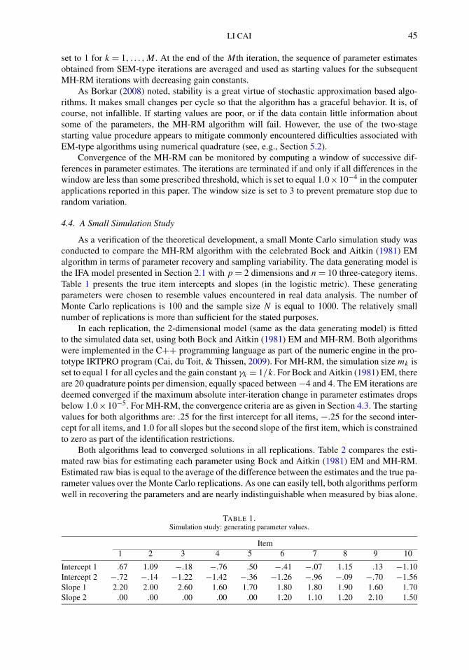
As a verification of the theoretical development, a small Monte Carlo simulation study wasconducted to compare the MH-RM algorithm with the celebrated Bock and Aitkin (1981) EMalgorithm in terms of parameter recovery and sampling variability. The data generating model isthe IFA model presented in Section 2.1 with p = 2 dimensions and n = 10 three-category items.Table 1 presents the true item intercepts and slopes (in the logistic metric). These generatingparameters were chosen to resemble values encountered in real data analysis. The number ofMonte Carlo replications is 100 and the sample size N is equal to 1000. The relatively smallnumber of replications is more than sufficient for the stated purposes.

In each replication, the 2-dimensional model (same as the data generating model) is fittedto the simulated data set, using both Bock and Aitkin (1981) EM and MH-RM. Both algorithmswere implemented in the C++ programming language as part of the numeric engine in the pro-totype IRTPRO program (Cai, du Toit, & Thissen, 2009). For MH-RM, the simulation size mk isset to equal 1 for all cycles and the gain constant γk = 1/k. For Bock and Aitkin (1981) EM, thereare 20 quadrature points per dimension, equally spaced between −4 and 4. The EM iterations aredeemed converged if the maximum absolute inter-iteration change in parameter estimates dropsbelow 1.0×10−5. For MH-RM, the convergence criteria are as given in Section 4.3. The startingvalues for both algorithms are: .25 for the first intercept for all items, −.25 for the second inter-cept for all items, and 1.0 for all slopes but the second slope of the first item, which is constrainedto zero as part of the identification restrictions.

Both algorithms lead to converged solutions in all replications. Table 2 compares the esti-mated raw bias for estimating each parameter using Bock and Aitkin (1981) EM and MH-RM.Estimated raw bias is equal to the average of the difference between the estimates and the true pa-rameter values over the Monte Carlo replications. As one can easily tell, both algorithms performwell in recovering the parameters and are nearly indistinguishable when measured by bias alone.

TABLE 1.Simulation study: generating parameter values.

Item1 2 3 4 5 6 7 8 9 10

Intercept 1 .67 1.09 −.18 −.76 .50 −.41 −.07 1.15 .13 −1.10Intercept 2 −.72 −.14 −1.22 −1.42 −.36 −1.26 −.96 −.09 −.70 −1.56Slope 1 2.20 2.00 2.60 1.60 1.70 1.80 1.80 1.90 1.60 1.70Slope 2 .00 .00 .00 .00 .00 1.20 1.10 1.20 2.10 1.50

46 PSYCHOMETRIKA

TABLE 2.Simulation study: raw bias (Monte Carlo standard deviations).

Item Intercept 1 Intercept 2 Slope 1 Slope 2BAEM MHRM BAEM MHRM BAEM MHRM BAEM MHRM

1 .00 (.13) −.01 (.13) −.02 (.12) −.02 (.12) .03 (.20) .02(.20) N/A N/A2 .01 (.13) .00 (.13) .00 (.12) .00 (.12) .02 (.17) .02(.17) −.01 (.15) −.01 (.14)

3 −.01 (.13) −.01 (.13) .00 (.14) .00 (.14) −.01 (.21) −.01(.21) .04 (.18) .03 (.17)

4 −.01 (.09) −.01 (.09) −.01 (.11) −.01 (.11) .00 (.13) .00(.13) .00 (.12) −.01 (.11)

5 −.01 (.10) −.01 (.10) .00 (.10) −.01 (.10) .01 (.14) .01(.14) .00 (.13) .00 (.12)

6 .00 (.12) −.01 (.12) −.03 (.14) −.03 (.14) .01 (.17) .01(.17) .03 (.16) .02 (.16)

7 −.01 (.11) −.01 (.11) −.01 (.10) −.01 (.10) .00 (.14) .00(.14) −.01 (.16) −.01 (.15)

8 .00 (.13) .00 (.13) .00 (.12) .00 (.12) −.01 (.16) −.01(.16) .02 (.16) .01 (.15)

9 .00 (.13) .00 (.13) .00 (.13) −.01 (.13) −.01 (.19) .00(.18) .02 (.30) .03 (.31)

10 −.02 (.13) −.02 (.13) −.02 (.13) −.02 (.13) .02 (.18) .03 (.18) .02 (.21) .02 (.21)

Note. BAEM = Bock–Aitkin EM algorithm; Bias is defined as the Monte Carlo average of estimates minusthe corresponding true value; Monte Carlo Standard Deviations are in the parentheses. Slope 2 of item 1 isfixed to 0 as part of the identification constraints.

Also contained in Table 2 is the information about sampling variability. Specifically, the MonteCarlo standard deviations, defined as the observed standard deviations of the estimates overMonte Carlo replications, are again nearly indistinguishable between Bock and Aitkin (1981)EM and MH-RM. The total root mean square deviation from true values for all parameters isequal to .014 for both algorithms. The average of per replication run time is 30 seconds for Bockand Aitkin (1981) EM and 41 seconds for MH-RM. The simulation suggests that the maximumlikelihood solutions produced by the Bock and Aitkin (1981) EM algorithm and the MH-RMalgorithm have comparable quality, though for sufficiently low-dimensional problems, a fullyoptimized deterministic algorithm such as EM can be more efficient.

5. Numerical Illustrations

To examine the empirical performance of MH-RM, two sets of data were analyzed in a com-parison of the proposed algorithm with well-established alternatives that include a Gibbs sam-pling based MCMC estimation algorithm (Section 5.1) and an adaptive Gauss–Hermite quadra-ture based EM algorithm (Section 5.2). To ensure fairness, only compiled native-code softwareprograms written in a high-level language such as FORTRAN or C++ are used in the compar-ison. For MH-RM, the prototype IRTPRO (Cai et al., 2009) is used. The Gibbs sampling basedMCMC method developed and implemented by Edwards (2005) is chosen because the C++ pro-gram (MultiNorm) was specifically designed for item factor analysis. The adaptive quadratureEM module in IRTPRO (Cai et al., 2009) is also used because of its exclusive focus on item fac-tor analysis. While Mplus 5.0 (Muthén & Muthén, 2008) is less focused on item factor analysis,it serves as an independent benchmark in comparisons involving EM due to its wide availability.CEFA (Browne, Cudeck, Tateneni, & Mels, 2008) is used for factor rotation. All analyses wereconducted on a laptop computer with a 2 GHz Intel Duo Core CPU and 2 GB of RAM. Parallelprocessing on multi-core or hyper-threaded CPUs is directly supported in IRTPRO and Mplus,but the capability is turned off in the comparisons.

5.1. MCMC for a Simulated Data Set

The data are the responses of 2000 simulees to a hypothetical scale consisting of 194-category graded items. There are four correlated factors underlying the item responses. The

LI CAI 47

TABLE 3.Rotated factor loadings for simulated data with generating values as the target.

Item Factor 1 Factor 2 Factor 3 Factor 4Gen MH MC Gen MH MC Gen MH MC Gen MH MC

1 .82 .87 .86 0 −.05 .00 0 .08 −.02 0 −.09 −.042 .84 .82 .85 0 .00 −.04 0 .02 .08 0 .03 −.053 .78 .76 .79 0 .06 −.01 0 −.02 .00 0 .00 .014 .69 .69 .67 0 .02 .04 0 −.07 −.04 0 .09 .075 .77 .75 .72 0 .03 .04 0 −.03 −.02 0 .03 .046 0 −.07 −.07 .81 .85 .85 0 −.05 −.04 0 .07 .057 0 .04 .05 .73 .71 .70 0 −.05 −.04 0 .04 .038 0 .08 .05 .65 .60 .63 0 .09 .04 0 −.14 −.079 0 .00 .00 .77 .78 .77 0 −.01 .01 0 −.03 −.04

10 0 −.02 −.02 .76 .73 .74 0 .06 .04 0 −.01 −.0211 0 .02 .02 0 .02 .01 .86 .79 .79 0 .06 .0512 0 −.02 −.01 0 .04 .03 .88 .83 .81 0 .05 .0513 0 .01 .02 0 −.04 −.05 .80 .86 .86 0 −.05 −.0514 0 −.01 −.01 0 .00 −.01 .74 .77 .78 0 −.03 −.0315 0 −.03 −.03 0 .02 .02 .78 .77 .78 0 .03 .0116 0 −.01 −.01 0 −.05 −.05 0 .06 .05 .78 .76 .7617 0 −.01 .00 0 .04 .02 0 −.06 −.05 .78 .83 .8118 0 −.03 −.02 0 .04 .01 0 .04 .05 .69 .62 .6119 0 .10 .04 0 −.09 −.02 0 .03 −.02 .63 .57 .61

Note. Gen = Generating values serving as the target; MH = target rotated MH-RM estimates; MC = targetrotated MCMC estimates.

TABLE 4.Factor correlations after target rotation for simulated data.

Factor Correlations (i, j)

(2,1) (3,1) (3,2) (4,1) (4,2) (4,3)

Generating Value .75 .70 .75 .60 .50 .80MH-RM Estimates .73 .67 .73 .62 .52 .79MCMC Estimates .74 .68 .75 .64 .56 .81

first three factors are each measured by 5 items and the last one by 4 items. The details for datasimulation can be found in Edwards (2005) and Table 3 lists the generating factor pattern.

For MH-RM, the simulation size mk is set to 1 and the gain constants γk = 1/k, with thesame convergence criteria as given in Section 4.3. For the MCMC method, a total of 60,000random draws were taken with diffuse priors on all item parameters. The first 10,000 drawsare regarded as “burn-in” and the “thinning” interval is 50. As noted by Edwards (2005), theseconservative choices ensure that the results are not dependent on the peculiarities of the startingvalues. The posterior means of the item parameters can be understood as approximate MLEs.

Given the availability of the generating parameters, a completely specified oblique targetrotation (Browne, 2001) of the estimated factor loadings can be applied to both solutions, with thegenerating loadings serving as the target. A side-by-side comparison of the target rotated loadingsare presented in Table 3, and a similar comparison of the factor correlations is available in Table 4.As can be seen, the MH-RM and MCMC estimates are very close to each other and both are closeto the generating values. The Root Mean Square Deviation (RMSD) from target for MH-RM is0.046 and the RMSD for MCMC is 0.039. It is worth noting that IRTPRO uses the logisticparameterization and MultiNorm uses the normal ogive parameterization. In addition, IRTPRO

48 PSYCHOMETRIKA

TABLE 5.Item wording for the social quality of life scale.

Wording

Item 1 I could talk with my friends.Item 2 I felt good about how I got along with classmates.Item 3 I felt comfortable with other kids my age.Item 4 I felt loved by my parents or guardians.Item 5 I was good at making friends.Item 6 Other kids wanted to be with me.Item 7 I felt accepted by other kids my age.Item 8 I did things with other kids my age.Item 9 I was good at talking with adults.

Item 10 My teachers understood me.Item 11 I wanted to spend time with my family.Item 12 I had problems getting along with my parents or guardians.Item 13 I got into a yelling fight with other kids.Item 14 I had trouble getting along with my family.Item 15 Other kids made fun of me.Item 16 I felt bad about how I got along with my friends.Item 17 I felt different from other kids my age.Item 18 Other kids were mean to me.Item 19 I felt nervous when I was with other kids my age.Item 20 I did not want to be with other kids.Item 21 I had trouble getting along with other kids my age.Item 22 I got along better with adults than with other kids my age.Item 23 I was afraid of other kids my age.Item 24 I wished I had more friends.

explicitly optimizes a log-likelihood while MultiNorm does not. These numerical differencesmay have contributed to the .007 difference in RMSDs. There is, however, a large difference incomputational time. MH-RM required 47 seconds of run time in 197 cycles and MCMC required1 hour 20 minutes and 34 seconds of run time.

5.2. A Social Quality of Life Scale for Children

The data are the responses of 753 children (between the ages of 8 to 17) to 24 social qualityof life items on an item tryout form for the Pediatric Quality of Life scales. Table 5 lists the textof item wording. The five-point response scale is “Never” (0), “Almost never” (1), “Sometimes”(2), “Often” (3), and “Almost Always” (4). The item responses have been recoded if necessaryso that the highest numerical value of the response scale indicates positive social quality of life.

The adaptive quadrature based EM implementation in IRTPRO is used. The convergencecriterion for EM considers a solution converged when the interiteration change in log-likelihooddrops below .001. For MH-RM, the simulation size mk is again set to 1 and the gain constantsγk = 1/k, with the same convergence criteria as in the previous sections.

5.2.1. A Unidimensional Model. Initial calibration of the items using a unidimensionalgraded response model suggests that the model fits the data poorly and there is strong indi-cation of local dependence. The unidimensional graded model is a special case of the gradedIFA model with a single latent variable (p = 1). For numerical integration, 21 adaptive Gauss–Hermite quadrature points are used so that the log-likelihood can be approximated accurately.

Table 6 shows a side-by-side comparison of the two sets of item parameter estimates (inlogistic metric) obtained from the two algorithms. The EM algorithm required 5 seconds of run

LI CAI 49

TABLE 6.Unidimensional graded model parameter estimates.

Item Intercept 1 Intercept 2 Intercept 3 Intercept 4 Slope (SE)MH-RM EM MH-RM EM MH-RM EM MH-RM EM MH-RM EM

1 3.32 3.32 2.60 2.61 .82 .82 −.09 −.08 1.31 (.10) 1.31 (.11)

2 3.07 3.07 2.19 2.19 .56 .56 −.59 −.59 .11 (.07) .11 (.07)

3 3.42 3.42 2.70 2.71 .77 .77 −.40 −.39 .73 (.08) .73 (.09)

4 4.53 4.53 3.72 3.72 1.88 1.89 .35 .36 1.62 (.13) 1.62 (.13)

5 3.28 3.28 2.58 2.59 1.03 1.04 −.39 −.38 1.32 (.10) 1.31 (.11)

6 3.42 3.42 2.46 2.46 .79 .79 −.41 −.40 .93 (.09) .92 (.09)

7 4.14 4.13 3.14 3.14 1.10 1.10 −.60 −.59 1.96 (.13) 1.94 (.14)

8 3.45 3.45 2.66 2.66 1.13 1.13 .11 .12 .82 (.09) .82 (.09)

9 3.58 3.59 2.94 2.95 1.54 1.56 .17 .18 1.67 (.12) 1.67 (.13)

10 4.04 4.05 3.77 3.78 2.74 2.74 1.62 1.63 .84 (.12) .85 (.12)

11 4.65 4.65 3.91 3.91 2.65 2.66 1.33 1.34 1.22 (.13) 1.23 (.13)

12 4.22 4.23 3.30 3.30 1.70 1.70 .21 .21 1.71 (.12) 1.71 (.13)

13 3.88 3.88 2.71 2.72 1.07 1.08 −.05 −.04 1.70 (.12) 1.70 (.13)

14 2.52 2.52 1.60 1.60 −.28 −.27 −1.24 −1.24 .87(.08) .87 (.09)

15 3.93 3.95 3.26 3.28 1.50 1.51 .19 .20 1.69 (.13) 1.70 (.13)

16 3.61 3.61 2.91 2.92 1.20 1.21 .12 .13 .91 (.09) .91 (.09)

17 3.65 3.64 2.69 2.69 1.23 1.23 −.14 −.14 .71 (.09) .70 (.09)

18 4.46 4.47 3.85 3.86 1.77 1.78 .26 .27 1.88 (.14) 1.88 (.14)

19 3.98 4.00 3.12 3.13 1.81 1.83 .47 .47 1.33 (.11) 1.34 (.12)

20 4.72 4.72 3.61 3.62 1.74 1.75 .33 .34 1.48 (.11) 1.48 (.12)

21 4.42 4.43 3.43 3.44 1.81 1.82 .55 .55 1.48 (.12) 1.49 (.13)

22 4.64 4.65 4.03 4.05 2.78 2.80 1.38 1.40 1.62 (.14) 1.63 (.15)

23 4.20 4.20 3.61 3.62 1.22 1.23 −.55 −.55 1.51 (.11) 1.51 (.12)

24 4.17 4.17 3.20 3.21 1.60 1.61 .04 .05 1.32 (.11) 1.32 (.11)

time in 47 cycles. The MH-RM algorithm required 10 seconds of run time in 128 cycles. Ascan be seen from Table 6, the two sets of estimates are nearly identical. The absolute differencebetween EM estimates and MH-RM estimates is no larger than .02. The standard errors of theslopes are also quite similar. The observed data log-likelihood is equal to −19590.4, accordingto EM. For MH-RM, the value is −19590.2. In this case there is no real difference in the qualityof estimates. As expected, MH-RM is less efficient than EM for this unidimensional problem.

5.2.2. A Five-Dimensional Model. The combination of expert advice, the wording of theitems in Table 5, as well as the existence of such problematic cases as Item #2 in the initialcalibration suggests that there may well be additional dimensions underlying the 24-item scale.IFA is a useful tool for modeling these extra dimensions. Specifically, an IFA model with 5 latentvariables in a pseudo-bifactor structure seems plausible.

The approach taken here is conventional. One first fits an exploratory IFA model with 5 fac-tors to the data, and then rotates the loadings orthogonally to a partially-specified target (Browne,2001). Plausibility of the hypothesized factor structure can be inferred from the RMSD of the ro-tated loadings from the target. Table 7 shows this target pattern. The entries in the table that aremarked with an X indicate unspecified loadings whose magnitude is to be determined by rota-tion, whereas the 0s indicate loadings to be minimized by the target rotation. The first factor canbe regarded as a primary social quality of life dimension. The other factors mainly account forextra local dependence.

Once again, both the MH-RM algorithm and the EM algorithm are used for fitting the IFAmodel. Due to an increase in the number of factors, the number of quadrature points per dimen-

50 PSYCHOMETRIKA

TABLE 7.Target rotated factor loadings.

Item Factor 1 Factor 2 Factor 3 Factor 4 Factor 5TP MH EM TP MH EM TP MH EM TP MH EM TP MH EM

1 X .62 .61 0 .14 .14 0 −.12 −.10 0 .04 .01 0 .02 .022 X .00 −.01 0 .19 .19 X .40 .39 0 .18 .17 0 −.13 −.113 X .28 .29 X .38 .36 0 .09 .09 X .32 .36 0 .06 .044 X .57 .57 X .47 .46 0 .01 .00 0 .16 .16 0 −.06 −.055 X .61 .61 0 .08 .08 0 .02 .02 0 −.01 −.01 0 .06 .056 X .52 .52 0 −.08 −.08 X .55 .55 0 .02 .02 0 .05 .047 X .76 .76 0 .05 .04 0 −.09 −.09 0 .06 .06 X .55 .578 X .44 .45 0 −.04 −.04 0 .24 .24 0 −.01 .00 0 .27 .259 X .55 .55 X .52 .52 0 −.08 −.08 0 .07 .06 0 .01 .02

10 X .29 .29 X .44 .45 X .43 .44 X .34 .31 0 −.03 −.0111 X .73 .73 0 −.16 −.15 0 −.17 −.17 0 .30 .29 0 −.09 −.0812 X .72 .72 0 −.01 −.02 0 .02 .02 0 .00 .00 X .51 .5013 X .75 .75 0 −.01 .00 0 .06 .05 0 −.08 −.08 0 .13 .1214 X .50 .50 0 .01 .01 0 −.03 −.03 X −.51 −.53 0 −.05 −.0515 X .56 .56 X .54 .53 0 −.06 −.06 0 .04 .03 0 .01 .0116 X .34 .35 X .34 .34 0 .28 .28 0 −.01 .00 0 .10 .0917 X .43 .43 0 −.08 −.09 X .68 .68 0 −.05 −.04 0 .00 −.0218 X .56 .56 X .56 .55 0 .16 .17 0 −.03 −.04 0 .09 .0819 X .65 .66 0 .01 .02 0 .19 .19 0 −.19 −.18 0 −.04 −.0520 X .75 .76 0 −.03 −.03 0 −.03 −.05 0 −.01 .01 0 −.15 −.1521 X .69 .69 0 .09 .09 0 .04 .03 0 −.15 −.14 0 −.08 −.0822 X .53 .52 X .56 .57 0 −.05 −.05 0 −.04 −.05 0 −.05 −.0423 X .50 .51 X .56 .56 0 −.12 −.12 0 −.04 −.03 0 .01 .0124 X .46 .47 X .57 .57 0 −.13 −.13 0 −.11 −.11 0 −.07 −.07

Note. TP = Target Pattern, where X indicates unspecified elements whose magnitude is determined byrotation; MH = target rotated MH-RM estimates; EM = target rotated EM estimates.

sion is reduced to 5 in EM. Thus, the E-step needs a total of 55 = 3125 function evaluations forthe integral approximation. The EM algorithm required 1 hours 27 minutes of run time in 301cycles. The MH-RM algorithm required 95 seconds of run time in 540 cycles. The EM algorithmused over 50 times more CPU time than MH-RM.

Table 7 compares the rotated factor loadings obtained from MH-RM and EM. Both solutionsgenerally fit within the hypothesized structure and are close to each other. The overall RMSDfrom target is equal to .103 for MH-RM and .101 for EM. Note that the factor pattern presentedhere is just one possible solution and there is nothing irrevocable about the target pattern. TheMH-RM solution has a log-likelihood of −18967.4, which is very close to the height of thelog-likelihood (−18968.7) that the EM algorithm attained.

5.3. Independent Verifications

Mplus (Muthén & Muthén, 2008) is used to independently verify the solutions obtained byIRTPRO’s EM module for the social quality of life data. Also of interest is the run time. Figure 1shows a head-to-head comparison of the computing time of the three approaches (MH-RM inIRTPRO, EM in IRTPRO, and EM in Mplus), varying the numbers of factors extracted. For theunidimensional model, 21 quadrature points are used; for all other number of factors, there are5 quadrature points per dimension. While the estimates as well as the log-likelihood values arevirtually identical for all three programs, large difference in computing time surfaced for 4- and

LI CAI 51

FIGURE 1.Program run time comparisons. IRTPRO-MH-RM denotes the implementation of MH-RM algorithm in IRTPRO. IRT-PRO-ADQEM denotes the implementation of the adaptive quadrature based EM algorithm in IRTPRO. Mplus-ADQEMdenotes the implementation of the adaptive quadrature based EM algorithm in Mplus.

5-dimensional models. One can clearly see that the computing time for adaptive quadrature basedEM is exponentially increasing while that of MH-RM grows only linearly as more factors areextracted. As witnessed in the simulation study in Section 4.4, for sufficiently low dimensionalproblems, MH-RM can be less efficient than EM, but in those situations, the absolute amountof time required is not large; whereas for high-dimensional problems, MH-RM can be far moreefficient than EM because it does not involve numerical quadrature.

6. Extensions

6.1. Confirmatory Item Factor Analysis

Confirmatory item factor analysis is ideal when there exists sufficient prior theory aboutthe factor structure of the items. The MCMC sampling procedure and the RM step in the pro-posed MH-RM algorithm remain the same as before. The constraints on the item parametersare imposed on the complete data log-likelihood. Estimation of the factor inter-correlations isstraightforward because the complete data likelihood consists of two independent parts (seeEquation (8)) so that the estimation of population distribution parameters is separate from theestimation of item parameters.

6.2. Explanatory and Multilevel IRT

Recent interest in generalizing the standard IRT model to include covariate effects, possi-bly even random-effects, has called for new estimation algorithms (de Boeck & Wilson, 2004;Fox & Glas, 2001; Fox, 2003, 2005). The MH-RM algorithm is uniquely suited to the goal offinding the MLEs for these extended IRT models because once the latent variables are “filled-in,”the complete data model often takes the form of a generalized linear model. For instance, in ex-planatory IRT one can allow the item difficulty and slope parameters to depend on an observedcovariate. The MH-RM solution to this problem simply involves conditioning on the covariate inaddition to the observed response patterns when generating the factor score imputations, in whichcase the complete data model is specified as a generalized linear model with main effects for thecovariate and the factor scores, as well as a term for their interaction. For multilevel IRT, thecluster-level random-effects induced by the random regression coefficients can also be thought

52 PSYCHOMETRIKA

of as missing data that must be imputed along with the factor scores. In this case the completedata model usually reduces to a generalized linear model with an “offset” term (McCullagh &Nelder, 1989).

6.3. Other Types of Models

The MH-RM algorithm as implemented in its current form is designed with efficient itemfactor analysis as the primary objective. However, the algorithm can in principle be applied tofit more general kinds of latent variables models such as the comprehensive structural equationmodel proposed by Muthén (1984), the generalized linear latent variable model of Bartholomewand Knott (1999), and the GLLAMM model of Rabe-Hesketh, Skrondal, and Pickles (2004b). Itis also worth noting that because item response theory models can be represented as nonlinearmixed-effects models (de Boeck & Wilson, 2004), the MH-RM algorithm may turn out to bea useful computational tool for parameter estimation in general nonlinear multilevel models.The SAEM algorithm, a close relative of the MH-RM algorithm (see Section 3.3), was initiallyintended for the mixture problem (Celeux & Diebolt, 1991). Thus, it is conceivable that theMH-RM may be extended to the case of categorical latent variables.

7. Discussion

This paper is concerned with the theoretical properties, implementation details, and empiri-cal performance of a new parameter estimation algorithm for computing the MLE in the contextof high-dimensional item factor analysis. The Metropolis–Hasting Robbins–Monro algorithm isa juxtaposition of elements from MCMC and stochastic approximation that appears to be moreefficient than quadrature based EM for high-dimensional problems. For practical data analysis,the decrease in computational burden as witnessed in Section 5 translates into increase in pro-ductivity. Though the highest number of dimensions reported in the empirical applications inthis paper is only five, Cai (2008a) already applied MH-RM successfully to problems with evenhigher dimensionality, where the speed difference is even more striking.

Before Bock and Aitkin (1981), the Bock and Lieberman (1970) style Newton algorithmsimply could not handle the number of items that one encounters in day-to-day data analysis fortesting situations. The EM algorithm due to Bock and Aitkin (1981) made IRT modeling practicalfor educational and psychological measurement. As IRT continues to evolve, high-dimensionalIFA has become a valuable tool in at least some of its new domains of application, e.g., mentalhealth and outcomes research. MH-RM provides a promising solution to the challenging numer-ical problems that arise from high-dimensional IFA. More research is still needed to study itsbehavior in a wide variety of situations and for models other than IFA.

Open Access This article is distributed under the terms of the Creative Commons Attribution Noncommercial Licensewhich permits any noncommercial use, distribution, and reproduction in any medium, provided the original author(s) andsource are credited.

Appendix A. The Convergence of MH-RM

The method for showing the convergence of the MH-RM algorithm relies on an OrdinaryDifferential Equation (ODE) argument that has become the predominant approach in the Sto-chastic Approximation literature (see Benveniste et al., 1990; Borkar, 2008; Kushner & Yin,1997). It is instructive to illustrate this technique with the original Robbins–Monro algorithm.Equation (13) can be rewritten as a stochastic difference equation:

θk+1 = θk + γkg(θk) + γkζk+1, (25)

LI CAI 53

where the last part γkζk+1 has mean zero and is independent from the past, so it can be thoughtof as a disturbance term. Due to the assumptions on the decaying gain constants, the asymptoticeffect of the disturbance term can be regarded as negligible as k tends to infinity. Thus, when k

is large and consequently γk is small, the remaining parts of (25) becomes

θk+1 = θk + γkg(θk). (26)

Equation (26) can be considered a discrete approximation to the trajectory of the following ODE:

dθ(t)

dt= g

(θ(t)

), (27)

similar to Euler’s scheme for numerically integrating (27) given initial values (θ0, g(θ0)):

θk+1 = θk + γg(θk). (28)

As long as the ODE (27) is well posed, which is usually the case for realistic models and appli-cations, the root-finding problem amounts to finding the equilibrium solution of the ODE. Usingthe foregoing argument, the Robbins–Monro recursions can be shown to asymptotically (in time)track the ODE with probability one (see, e.g., Borkar, 2008). Thus, the Robbins–Monro sequenceshould converge to a stable equilibrium of (27) and the root of g(θ) = 0 can be found withouteven explicitly knowing the precise form of g(·).

Returning to the MH-RM algorithm, recall that Z = (Y,X). Reference to Y will be sup-pressed because it is fixed once observed. To avoid intricate notation, it is sufficient to considermk = 1 for all k. Let

H̄(θ) =∫

EH(θ |Z)�(dX|θ), and s̄(θ) =

∫E

s(θ |Z)�(dX|θ).

Inspection of the stochastic difference equations (17) and (18) shows that the following set ofODEs govern the asymptotic (in time) behavior of MH-RM:( ∂

∂tθ(t)

∂∂t

(t)

)=

((t)−1s̄(θ(t))

H̄(θ(t)) − (t)

),

(θ(0)

(0)

)=

(θ

). (29)

It can be verified that for MLE θ̂ , the point (θ̂ , H̄(θ̂)) is a stable equilibrium of the ODE (29).Therefore, the sequence of estimates generated by the MH-RM method converges to the MLE:

θ (k) → θ̂, with probability 1 as k → ∞. (30)

This result is a direct consequence of Gu and Kong (1998) Theorem 1, which is in turn based ongeneral convergence results in Benveniste et al. (1990). The conditions needed for the conver-gence to hold are the same as those in Gu and Kong (1998) Theorem 1. These conditions guar-antee (a) the integrability, convergence, and continuity of the Markov transition kernel, (b) thecontinuity and the existence of sufficient moments for functions H(θ |Z) and s(θ |Z), and (c) thatthe process {(θ (k),k), k ≥ 1} as defined by Equation (18) is a bounded sequence.

Appendix B. Complete Data Log-Likelihood and Derivatives

Suppressing references to i and j , the log-likelihood under consideration can be writtenusing simplified notation as

l =C−1∑k=0

χk(y) log(Pk − Pk+1), (31)

54 PSYCHOMETRIKA

where Pk = P(y ≥ k|θ ,x) is as defined in Equation (1). The first derivatives of (31) are

∂l

∂αk

= −(

χk−1(y)

Pk−1 − Pk

− χk(y)

Pk − Pk+1

)∂Pk

∂αk

,

∂l

∂β=

C−1∑k=0

χk(y)

Pk − Pk+1

(∂Pk

∂β− ∂Pk+1

∂β

),

where ∂Pk/∂αk = Pk(1 − Pk), ∂Pk/∂β = Pk(1 − Pk)x. The second derivatives are given by

∂2l

∂α2k

= −(

χk−1(y)

(Pk−1 − Pk)2+ χk(y)

(Pk − Pk+1)2

)(∂Pk

∂αk

)2

−(

χk−1(y)

Pk−1 − Pk

− χk(y)

Pk − Pk+1

)(∂

∂αk

∂Pk

∂αk

),

∂2l

∂γk−1∂αk

= χk−1(y)

(Pk−1 − Pk)2

(∂Pk−1

∂γk−1

)(∂Pk

∂αk

),

∂2l

∂γk+1∂αk

= χk(y)

(Pk − Pk+1)2

(∂Pk+1

∂γk+1

)(∂Pk

∂αk

),

∂2l

∂β∂αk

= − χk(y)

(Pk − Pk+1)2

(∂Pk

∂αk

)(∂Pk

∂β− ∂Pk+1

∂β

)

+ χk−1(y)

(Pk−1 − Pk)2

(∂Pk

∂αk

)(∂Pk−1

∂β− ∂Pk

∂β

)

−(

χk−1(y)

Pk−1 − Pk

− χk(y)

Pk − Pk+1

)(∂

∂β

∂Pk

∂αk

),

∂2l

∂β∂β ′ =C−1∑k=0

{− χk(y)

(Pk − Pk+1)2

(∂Pk

∂β− ∂Pk+1

∂β

)(∂Pk

∂β ′ − ∂Pk+1

∂β ′)

+ χk(y)

Pk − Pk+1

(∂

∂β

∂Pk

∂β ′ − ∂

∂β

∂Pk+1

∂β ′)}

,

where

∂

∂αk

∂Pk

∂αk

= Pk(1 − Pk)(1 − 2Pk),

∂

∂β

∂Pk

∂αk

= Pk(1 − Pk)(1 − 2Pk)x,

∂

∂β

∂Pk

∂β ′ = Pk(1 − Pk)(1 − 2Pk)xx′.

References

Albert, J.H. (1992). Bayesian estimation of normal ogive item response curves using Gibbs sampling. Journal of Educa-tional Statistics, 17, 251–269.

Aptech Systems, Inc. (2003). GAUSS (Version 6.08) [Computer software]. Maple Valley: Author.Baker, F.B., & Kim, S.-H. (2004). Item response theory: Parameter estimation techniques. New York: Dekker.Bartholomew, D.J., & Knott, M. (1999). Latent variable models and factor analysis (2nd ed.). London: Arnold.

LI CAI 55

Bartholomew, D.J., & Leung, S.O. (2002). A goodness of fit test for sparse 2p contingency tables. British Journal ofMathematical and Statistical Psychology, 55, 1–15.

Béguin, A.A., & Glas, C.A.W. (2001). MCMC estimation and some model-fit analysis of multidimensional IRT models.Psychometrika, 66, 541–561.

Benveniste, A., Métivier, M., & Priouret, P. (1990). Adaptive algorithms and stochastic approximations. Berlin: Springer.Bishop, Y.M.M., Fienberg, S.E., & Holland, P.W. (1975). Discrete multivariate analysis: Theory and practice. Cam-

bridge: MIT Press.Bock, R.D., & Aitkin, M. (1981). Marginal maximum likelihood estimation of item parameters: Application of an EM

algorithm. Psychometrika, 46, 443–459.Bock, R.D., Gibbons, R., & Muraki, E. (1988). Full-information item factor analysis. Applied Psychological Measure-

ment, 12, 261–280.Bock, R.D., & Lieberman, M. (1970). Fitting a response model for n dichotomously scored items. Psychometrika, 35,

179–197.Bolt, D. (2005). Limited and full information estimation of item response theory models. In A. Maydeu-Olivares & J.J.

McArdle (Eds.), Contemporary psychometrics (pp. 27–71). Mahwah: Earlbaum.Booth, J.G., & Hobert, J.P. (1999). Maximizing generalized linear mixed model likelihoods with an automated Monte

Carlo EM algorithm. Journal of the Royal Statistical Society—Series B, 61, 265–285.Borkar, V.S. (2008). Stochastic approximation: A dynamical systems viewpoint. Cambridge: Cambridge University Press.Browne, M.W. (2001). An overview of analytic rotation in exploratory factor analysis. Multivariate Behavioral Research,

36, 111–150.Browne, M.W., Cudeck, R., Tateneni, K., & Mels, G. (2008). CEFA: Comprehensive Exploratory Factor Analysis (Ver-

sion 3.02) [Computer software]. Retrieved from http://quantrm2.psy.ohio-state.edu/browne/.Cai, L. (2006). Full-information item factor analysis by Markov chain Monte Carlo stochastic approximation. Unpub-

lished master’s thesis, Department of Statistics, University of North Carolina at Chapel Hill.Cai, L. (2008a). A Metropolis–Hastings Robbins–Monro algorithm for maximum likelihood nonlinear latent structure

analysis with a comprehensive measurement model. Unpublished doctoral dissertation, Department of Psychology,University of North Carolina at Chapel Hill.

Cai, L. (2008b). SEM of another flavour: Two new applications of the supplemented EM algorithm. British Journal ofMathematical and Statistical Psychology, 61, 309–329.

Cai, L., du Toit, S.H.C., & Thissen, D. (2009, forthcoming). IRTPRO: Flexible, multidimensional, multiple categoricalIRT modeling [Computer software]. Chicago: SSI International.

Cai, L., Maydeu-Olivares, A., Coffman, D.L., & Thissen, D. (2006). Limited-information goodness-of-fit testing ofitem response theory models for sparse 2p tables. British Journal of Mathematical and Statistical Psychology, 59,173–194.

Camilli, G. (1994). Origin of the scaling constant d = 1.7 in item response theory. Journal of Educational and BehavioralStatistics, 19, 379–388.

Celeux, G., Chauveau, D., & Diebolt, J. (1995). On stochastic versions of the EM algorithm (Tech. Rep. No. 2514).The French National Institute for Research in Computer Science and Control.

Celeux, G., & Diebolt, J. (1991). A stochastic approximation type EM algorithm for the mixture problem (Tech. Rep. No.1383). The French National Institute for Research in Computer Science and Control.

Chib, S., & Greenberg, E. (1995). Understanding the Metropolis-Hastings algorithm. The American Statistician, 49,327–335.

de Boeck, P., & Wilson, M. (2004). Explanatory item response models: A generalized linear and nonlinear approach.New York: Springer.

Delyon, B., Lavielle, M., & Moulines, E. (1999). Convergence of a stochastic approximation version of the EM algorithm.The Annals of Statistics, 27, 94–128.

Dempster, A.P., Laird, N.M., & Rubin, D.B. (1977). Maximum likelihood estimation from incomplete data via the EMalgorithm. Journal of the Royal Statistical Society—Series B, 39, 1–38.

Diebolt, J., & Ip, E.H.S. (1996). Stochastic EM: Method and application. In W.R. Gilks, S. Richardson, & D.J. Spiegel-halter (Eds.), Markov chain Monte Carlo in practice (pp. 259–273). London: Chapman and Hall.

Dunson, D.B. (2000). Bayesian latent variable models for clustered mixed outcomes. Journal of the Royal StatisticalSociety—Series B, 62, 355–366.

Edwards, M.C. (2005). A Markov chain Monte Carlo approach to confirmatory item factor analysis. Unpublished doc-toral dissertation, University of North Carolina at Chapel Hill.

Fisher, R.A. (1925). Theory of statistical estimation. Proceedings of the Cambridge Philosophical Society, 22, 700–725.Fox, J.-P. (2003). Stochastic EM for estimating the parameters of a multilevel IRT model. British Journal of Mathematical

and Statistical Psychology, 56, 65–81.Fox, J.-P. (2005). Multilevel IRT using dichotomous and polytomous response data. British Journal of Mathematical and

Statistical Psychology, 58, 145–172.Fox, J.-P., & Glas, C.A.W. (2001). Bayesian estimation of a multilevel IRT model using Gibbs sampling. Psychometrika,

66, 269–286.Gelfand, A.E., & Smith, A.F.M. (1990). Sampling-based approaches to calculating marginal densities. Journal of the

American Statistical Association, 85, 398–409.Gu, M.G., & Kong, F.H. (1998). A stochastic approximation algorithm with Markov chain Monte-Carlo method for

incomplete data estimation problems. The Proceedings of the National Academy of Sciences, 95, 7270–7274.Gu, M.G., Sun, L., & Huang, C. (2004). A universal procedure for parametric frailty models. Journal of Statistical

Computation and Simulation, 74, 1–13.

56 PSYCHOMETRIKA

Gu, M.G., & Zhu, H.-T. (2001). Maximum likelihood estimation for spatial models by Markov chain Monte Carlostochastic approximation. Journal of the Royal Statistical Society—Series B, 63, 339–355.

Gueorguieva, R.V., & Agresti, A. (2001). A correlated probit model for joint modeling of clustered binary and continuousresponses. Journal of the American Statistical Association, 96, 1102–1112.

Haberman, S.J. (1977). Log-linear models and frequency tables with small expected cell counts. The Annals of Statistics,5, 1148–1169.

Hastings, W.K. (1970). Monte Carlo simulation methods using Markov chains and their applications. Biometrika, 57,97–109.

Huber, P., Ronchetti, E., & Victoria-Feser, M.-P. (2004). Estimation of generalized linear latent variable models. Journalof the Royal Statistical Society—Series B, 66, 893–908.

Jank, W.S. (2004). Quasi-Monte Carlo sampling to improve the efficiency of Monte Carlo EM. Computational Statisticsand Data Analysis, 48, 685–701.

Joe, H. (2008). Accuracy of Laplace approximation for discrete response mixed models. Computational Statistics andData Analysis, 52, 5066–5074.

Kass, R., & Steffey, D. (1989). Approximate Bayesian inference in conditionally independent hierarchical models. Jour-nal of the American Statistical Association, 84, 717–726.

Kuhn, E., & Lavielle, M. (2005). Maximum likelihood estimation in nonlinear mixed effects models. ComputationalStatistics and Data Analysis, 49, 1020–1038.

Kullback, S., & Leibler, R.A. (1951). On information and sufficiency. Annals of Mathematical Statistics, 22, 79–86.Kushner, H.J., & Yin, G.G. (1997). Stochastic approximation algorithms and applications. New York: Springer.Lange, K. (1995). A gradient algorithm locally equivalent to the EM algorithm. Journal of the Royal Statistical Society—

Series B, 57, 425–437.Liu, Q., & Pierce, D.A. (1994). A note on Gauss–Hermite quadrature. Biometrika, 81, 624–629.Lord, F.M., & Novick, M.R. (1968). Statistical theories of mental test scores. Reading: Addison-Wesley.Louis, T.A. (1982). Finding the observed information matrix when using the EM algorithm. Journal of the Royal Statis-

tical Society—Series B, 44, 226–233.Makowski, D., & Lavielle, M. (2006). Using SAEM to estimate parameters of models of response to applied fertilizer.

Journal of Agricultural, Biological, and Environmental Statistics, 11, 45–60.Mardia, K.V., Kent, J.T., & Bibby, J.M. (1979). Multivariate analysis. San Diego: Academic Press.Maydeu-Olivares, A., & Cai, L. (2006). A cautionary note on using g2(dif) to assess relative model fit in categorical data

analysis. Multivariate Behavioral Research, 41, 55–64.Maydeu-Olivares, A., & Joe, H. (2005). Limited and full information estimation and testing in 2n contingency tables:

A unified framework. Journal of the American Statistical Association, 100, 1009–1020.McCullagh, P. (1980). Regression models for ordinal data. Journal of the Royal Statistical Society—Series B, 42,

109–142.McCullagh, P., & Nelder, J.A. (1989). Generalized linear models (2nd ed.). London: Chapman & Hall.McCulloch, C.E., & Searle, S.R. (2001). Generalized, linear, and mixed models. New York: Wiley.Meng, X.-L., & Schilling, S. (1996). Fitting full-information item factor models and an empirical investigation of bridge

sampling. Journal of the American Statistical Association, 91, 1254–1267.Metropolis, N., Rosenbluth, A.W., Rosenbluth, M.N., Teller, A.H., & Teller, E. (1953). Equations of state space calcula-

tions by fast computing machines. Journal of Chemical Physics, 21, 1087–1092.Mislevy, R.J. (1986). Bayes modal estimation in item response models. Psychometrika, 51, 177–195.Muthén, B. (1984). A general structural equation model with dichotomous, ordered categorical, and continuous latent

variable indicators. Psychometrika, 49, 115–132.Muthén, & Muthén (2008). Mplus (Version 5.0) [Computer software]. Los Angeles: Author.Natarajan, R., & Kass, R.E. (2000). Reference Bayesian methods for generalized linear mixed models. Journal of the

American Statistical Association, 95, 227–237.Naylor, J.C., & Smith, A.F.M. (1982). Applications of a method for the efficient computation of posterior distributions.

Journal of the Royal Statistical Society—Series C, 31, 214–225.Orchard, T., & Woodbury, M.A. (1972). A missing information principle: Theory and application. In L.M. Lecam, J. Ney-

man, & E.L. Scott (Eds.), Proceedings of the sixth Berkeley symposium on mathematical statistics and probability(pp. 697–715). Berkeley: University of California Press.

Patz, R.J., & Junker, B.W. (1999a). A straightforward approach to Markov chain Monte Carlo methods for item responsemodels. Journal of Educational and Behavioral Statistics, 24, 146–178.

Patz, R.J., & Junker, B.W. (1999b). Applications and extensions of MCMC in IRT: Multiple item types, missing data,and rated responses. Journal of Educational and Behavioral Statistics, 24, 342–366.

Rabe-Hesketh, S., Skrondal, A., & Pickles, A. (2004b). Generalized multilevel structural equation modeling. Psychome-trika, 69, 167–190.

Rabe-Hesketh, S., Skrondal, A., & Pickles, A. (2005). Maximum likelihood estimation of limited and discrete dependentvariable models with nested random effects. Journal of Econometrics, 128, 301–323.

Rabe-Hesketh, S., Skrondal, A., & Pickles, A. (2004a). GLLAMM manual (U.C. Berkeley Division of Biostatistics Work-ing Paper Series, 160).

Raudenbush, S.W., Yang, M.-L., & Yosef, M. (2000). Maximum likelihood for generalized linear models with nested ran-dom effects via high-order, multivariate Laplace approximation. Journal of Computational and Graphical Statistics,9, 141–157.

LI CAI 57

Reeve, B.B., Hays, R.D., Bjorner, J.B., Cook, K.F., Crane, P.K., Teresi, J.A., et al. (2007). Psychometric evaluationand calibration of health-related quality of life items banks: Plans for the patient-reported outcome measurementinformation system (PROMIS). Medical Care, 45, S22–31.

Robbins, H., & Monro, S. (1951). A stochastic approximation method. The Annals of Mathematical Statistics, 22,400–407.

Roberts, G.O., & Rosenthal, J.S. (2001). Optimal scaling for various Metropolis-Hastings algorithms. Statistical Science,16, 351–367.

Samejima, F. (1969). Estimation of latent ability using a response pattern of graded scores. Psychometric Monographs,17.

Savalei, V. (2006). Logistic approximation to the normal: The KL rationale. Psychometrika, 71, 763–767.Schilling, S., & Bock, R.D. (2005). High-dimensional maximum marginal likelihood item factor analysis by adaptive

quadrature. Psychometrika, 70, 533–555.Segall, D.O. (1998). IFACT computer program Version 1.0: Full information confirmatory item factor analysis using

Markov chain Monte Carlo estimation [Computer software]. Seaside: Defense Manpower Data Center.Shi, J.-Q., & Lee, S.-Y. (1998). Bayesian sampling-based approach for factor analysis models with continuous and

polytomous data. British Journal of Mathematical and Statistical Psychology, 51, 233–252.Song, X.-Y., & Lee, S.-Y. (2005). A multivariate probit latent variable model for analyzing dichotomous responses.

Statistica Sinica, 15, 645–664.te Marvelde, J., Glas, v.G.C., & van Damme, J. (2006). Application of multidimensional item response theory models to

longitudinal data. Educational and Psychological Measurement, 66, 5–34.Thissen, D. (2003). MULTILOG 7 user’s guide. Chicago: SSI International.Thomas, N. (1993). Asymptotic corrections for multivariate posterior moments with factored likelihood functions. Jour-

nal of Computational and Graphical Statistics, 2, 309–322.Tierney, L. (1994). Markov chains for exploring posterior distributions (with discussion). The Annals of Statistics, 22,

1701–1762.Tierney, L., & Kadane, J.B. (1986). Accurate approximations for posterior moments and marginal densities. Journal of

the American Statistical Association, 81, 82–86.Titterington, D.M. (1984). Recursive parameter estimation using incomplete data. Journal of the Royal Statistical

Society—Series B, 46, 257–267.Wainer, H., & Kiely, G. (1987). Item clusters and computerized adaptive testing: A case for testlets. Journal of Educa-

tional Measurement, 24, 185–202.Wei, G.C.G., & Tanner, M.A. (1990). A Monte Carlo implementation of the EM algorithm and the poor man’s data

augmentation algorithm. Journal of the American Statistical Association, 85, 699–704.Wirth, R.J., & Edwards, M.C. (2007). Item factor analysis: Current approaches and future directions. Psychological

Methods, 12, 58–79.Zhu, H.-T., & Lee, S.-Y. (2002). Analysis of generalized linear mixed models via a stochastic approximation algorithm

with Markov chain Monte-Carlo method. Statistics and Computing, 12, 175–183.Zimowski, M.F., Muraki, E., Mislevy, R.J., & Bock, R.D. (2003). BILOG-MG3 user’s guide. Chicago: SSI International.

Manuscript Received: 14 SEP 2008Final Version Received: 25 APR 2009Published Online Date: 28 JUL 2009