high dimensional sparse polynomial approximation of ... · with abdellah chkifa, ronald devore and...
TRANSCRIPT

High dimensional sparse polynomial approximationof parametric and stochastic PDE’s
Albert Cohen
Laboratoire Jacques-Louis LionsUniversite Pierre et Marie Curie
Paris
with Abdellah Chkifa, Ronald DeVore and Christoph Schwab
Bilbao 11-11-11

Motivation : parametric PDE’s
We are interested in PDE’s of the general form
F(u,y) = 0,
where F is a partial di!erential operator, u is the unknown and y = (yj)j=1,...,d is aparameter vector of dimension d >> 1 or d = +!.
The vector y may take any value in some domain U ! Rd .
We also assume well-posedness of the solution in some Banach space V for everyy " U,
y #" u(y)
is the solution map from U to V .
The parameters may be deterministic (control, optimization, inverse problems) orrandom (uncertainty modeling and propagation, reliability assessment).
These applications often requires many queries of u(y), and therefore in principlerunning many times a numerical solver.
Alternate approach : use a numerical approximation of the map y #" u(y).
Curse of dimensionality : approximation rates deteriorate as d " +!.
The curse of dimensionality
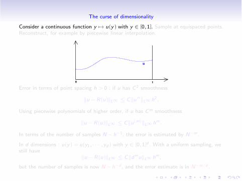
Consider a continuous function y #" u(y) with y " [0,1]. Sample at equispaced points.Reconstruct, for example by piecewise linear interpolation.
0 1
u
Error in terms of point spacing h > 0 : if u has C2 smoothness
$u !R(u)$L! % C$u !!$L! h2.
Using piecewise polynomials of higher order, if u has Cm smoothness
$u !R(u)$L! % C$u(m)$L! hm.
In terms of the number of samples N ! h!1, the error is estimated by N!m.
In d dimensions : u(y) = u(y1, · · · ,yd) with y " [0,1]d . With a uniform sampling, westill have
$u !R(u)$L! % C$dmu$L! hm,
but the number of samples is now N ! h!d , and the error estimate is in N!m/d .

The curse of dimensionality
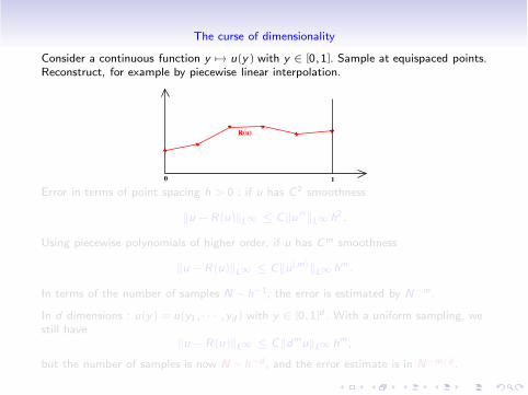
Consider a continuous function y #" u(y) with y " [0,1]. Sample at equispaced points.Reconstruct, for example by piecewise linear interpolation.
0 1
u
Error in terms of point spacing h > 0 : if u has C2 smoothness
$u !R(u)$L! % C$u !!$L! h2.
Using piecewise polynomials of higher order, if u has Cm smoothness
$u !R(u)$L! % C$u(m)$L! hm.
In terms of the number of samples N ! h!1, the error is estimated by N!m.
In d dimensions : u(y) = u(y1, · · · ,yd) with y " [0,1]d . With a uniform sampling, westill have
$u !R(u)$L! % C$dmu$L! hm,
but the number of samples is now N ! h!d , and the error estimate is in N!m/d .

The curse of dimensionality
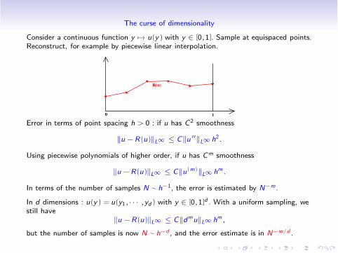
Consider a continuous function y #" u(y) with y " [0,1]. Sample at equispaced points.Reconstruct, for example by piecewise linear interpolation.
0 1
Error in terms of point spacing h > 0 : if u has C2 smoothness
$u !R(u)$L! % C$u !!$L! h2.
Using piecewise polynomials of higher order, if u has Cm smoothness
$u !R(u)$L! % C$u(m)$L! hm.
In terms of the number of samples N ! h!1, the error is estimated by N!m.
In d dimensions : u(y) = u(y1, · · · ,yd) with y " [0,1]d . With a uniform sampling, westill have
$u !R(u)$L! % C$dmu$L! hm,
but the number of samples is now N ! h!d , and the error estimate is in N!m/d .
The curse of dimensionality
Consider a continuous function y #" u(y) with y " [0,1]. Sample at equispaced points.Reconstruct, for example by piecewise linear interpolation.
0 1
R(u)
Error in terms of point spacing h > 0 : if u has C2 smoothness
$u !R(u)$L! % C$u !!$L! h2.
Using piecewise polynomials of higher order, if u has Cm smoothness
$u !R(u)$L! % C$u(m)$L! hm.
In terms of the number of samples N ! h!1, the error is estimated by N!m.
In d dimensions : u(y) = u(y1, · · · ,yd) with y " [0,1]d . With a uniform sampling, westill have
$u !R(u)$L! % C$dmu$L! hm,
but the number of samples is now N ! h!d , and the error estimate is in N!m/d .

Other sampling/reconstruction methods cannot do better
Can be explained by nonlinear manifold width (Alexandrov, DeVore-Howard-Micchelli).
Let X be a normed space and K ! X a compact set.
Consider maps E : K #" RN (encoding) and R : RN #" X (reconstruction).
Introducing the distorsion of the pair (E ,R) over K
maxu"K
$u !R(E(u))$X ,
we define the nonlinear N-width of K as
dN(K) := infE ,R
maxu"K
$u !R(E(u))$X ,
where the infimum is taken over all continuous maps (E ,R).
If X = L! and K is the unit ball of Cm([0,1]d ) it is known that
cN!m/d % dN(K) % CN!m/d .

Infinitely smooth functions
Nowak and Wosniakowski : if X = L! ([0,1]d ) and
K := {u " C! ([0,1]d) : $!"u$L! % 1 for all "}.
thenmin{N : dN(K) % 1/2} & c2d/2.
Conclusion : for high dimensional problems, smoothness properties of functions shouldbe revisited by other means than Cm classes, and appropriate approximation toolsshould be used.
Key ingredients :
(i) Sparsity
(ii) Variable reduction
(iii) Anisotropy

Our model example
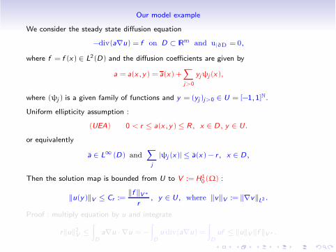
We consider the steady state di!usion equation
!div(a'u) = f on D ! IRm and u|!D = 0,
where f = f (x) " L2(D) and the di!usion coe"cients are given by
a = a(x,y) = a(x)+#
j>0
yj#j(x),
where (#j) is a given family of functions and y = (yj)j>0 " U = [!1,1]N.
Uniform ellipticity assumption :
(UEA) 0 < r % a(x,y) % R, x " D, y " U.
or equivalently
a " L! (D) and#
j
|#j (x)| % a(x)! r, x " D,
Then the solution map is bounded from U to V := H10 ($) :
$u(y)$V % Cr :=$f $V!
r, y " U, where $v$V := $'v$L2 .
Proof : multiply equation by u and integrate
r$u$2V %
$
Da'u ·'u = !
$
Du div(a'u) =
$
Duf % $u$V $f $V! .

Our model example
We consider the steady state di!usion equation
!div(a'u) = f on D ! IRm and u|!D = 0,
where f = f (x) " L2(D) and the di!usion coe"cients are given by
a = a(x,y) = a(x)+#
j>0
yj#j(x),
where (#j) is a given family of functions and y = (yj)j>0 " U = [!1,1]N.
Uniform ellipticity assumption :
(UEA) 0 < r % a(x,y) % R, x " D, y " U.
or equivalently
a " L! (D) and#
j
|#j (x)| % a(x)! r, x " D,
Then the solution map is bounded from U to V := H10 ($) :
$u(y)$V % Cr :=$f $V!
r, y " U, where $v$V := $'v$L2 .
Proof : multiply equation by u and integrate
r$u$2V %
$
Da'u ·'u = !
$
Du div(a'u) =
$
Duf % $u$V $f $V! .

Sparse polynomial approximations
We consider the expansion of u(y) =%
""F t"y" , where
y" :=
d&
j=1
y"j
j and t" :=1
"!!"u|y=0 " V with "! :=
d&
j=1
"j ! and 0! := 1.
where F = Nd , or F is the set of all finitely supported sequences of integers ifd = +! (finitely many "j (= 0). The sequence (t")""F is indexed by d >> 1 integers.
ν
1
ν3
2
ν
Objective : identify a set %! F with #(%) = N such that u is well approximated bythe partial expansion
u%(y) :=#
""%
t"y".

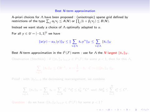
Best N-term approximation
A-priori choices for % have been proposed : (anisotropic) sparse grid defined byrestrictions of the type
%j &j"j % A(N) or
'j(1 +'j"j) % B(N).
Instead we want study a choice of % optimally adapted to u.
For all y " U = [!1,1]N we have
$u(y)!u%(y)$V % $#
"/"%
t"y"$V %#
"/"%
$t"$V
Best N-term approximation in the (1(F) norm : use for % the N largest $t"$V .
Observation (Stechkin) : if ($t"$V )""F " (p(F) for some p < 1, then for this %,
#
"/"%
$t"$V % CN!s , s :=1
p!1, C := $($t"$V )$p.
Proof : with (tn)n>0 the decreasing rearrangement, we combine
#
"/"%
$t"$V =#
n>N
tn =#
n>N
t1!pn tp
n % t1!pN Cp and Ntp
N %N#
n=1
tpn % Cp.
Question : do we have ($t"$V )""F " (p(F) for some p < 1 ?

The main result
Theorem (Cohen-DeVore-Schwab, Analysis and Application 2010) : under the uniformellipticity assumption (UAE), then for any p < 1,
($#j$L! )j>0 " (p(N) ( ($t"$V )""F " (p(F).
Interpretations :
(i) The Taylor expansion of u(y) inherits the sparsity properties of the expansion ofa(y) into the #j .
(ii) We approximate u(y) in L! (U) with algebraic rate )N<!N!s despite the curse of
(infinite) dimensionality, due to the fact that yj is less influencial as j gets large.
Such approximation rates cannot be proved for the usual a-priori choices of %.
Key idea in the proof : holomorphic extension u(y) " u(z) with z = (zj) " C|| IN.Domains of holomorphy : if * = (*j)j#0 is any positive sequence such that
#
j>0
*j |#j(x)| % a(x)!+, x " D,
for some + > 0, then u is holomorphic, with bound $u(z)$V % C+ =$f $V!
+, in polydisc
U* :=){|zj | % *j },
since "(a(x,z)) & + for z " U* .

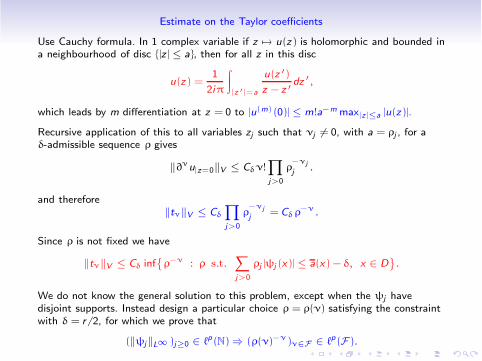
Estimate on the Taylor coe"cients
Use Cauchy formula. In 1 complex variable if z #" u(z) is holomorphic and bounded ina neighbourhood of disc {|z | % a}, then for all z in this disc
u(z) =1
2i,
$
|z "|=a
u(z !)
z ! z !dz !,
which leads by m di!erentiation at z = 0 to |u(m)(0)| % m!a!m max|z|%a |u(z)|.
Recursive application of this to all variables zj such that "j (= 0, with a = *j , for a+-admissible sequence * gives
$!"u|z=0$V % C+"!&
j>0
*!"j
j .
and therefore$t"$V % C+
&
j>0
*!"j
j = C+*!".
Since * is not fixed we have
$t"$V % C+ inf)*!" : * s.t.
#
j>0
*j |#j(x)| % a(x)!+, x " D*.
We do not know the general solution to this problem, except when the #j havedisjoint supports. Instead design a particular choice * = *(") satisfying the constraintwith + = r/2, for which we prove that
($#j$L! )j#0 " (p(N) ( (*(")!")""F " (p(F).
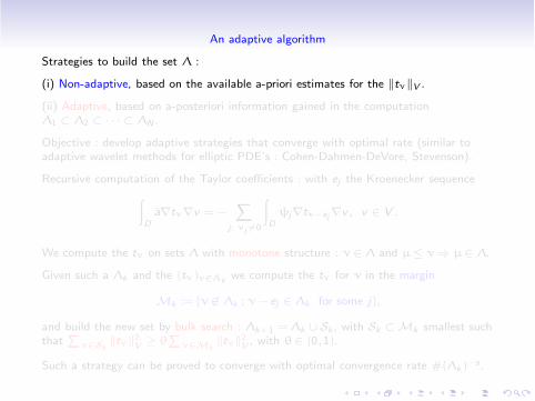
An adaptive algorithm
Strategies to build the set % :
(i) Non-adaptive, based on the available a-priori estimates for the $t"$V .
(ii) Adaptive, based on a-posteriori information gained in the computation%1 ! %2 ! · · · ! %N .
Objective : develop adaptive strategies that converge with optimal rate (similar toadaptive wavelet methods for elliptic PDE’s : Cohen-Dahmen-DeVore, Stevenson).
Recursive computation of the Taylor coe"cients : with ej the Kroenecker sequence
$
D
a't"'v = !#
j : "j &=0
$
D
#j't"!ej'v, v " V .
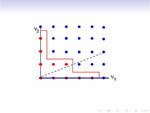
We compute the t" on sets % with monotone structure : " " % and µ% " ( µ" %.
Given such a %k and the (t")""%kwe compute the t" for " in the margin
Mk := {" /" %k ; "! ej " %k for some j},
and build the new set by bulk search : %k+1 = %k * Sk , with Sk ! Mk smallest suchthat
%""Sk
$t"$2V & -
%""Mk
$t"$2V , with -" (0,1).
Such a strategy can be proved to converge with optimal convergence rate #(%k)!s .

An adaptive algorithm
Strategies to build the set % :
(i) Non-adaptive, based on the available a-priori estimates for the $t"$V .
(ii) Adaptive, based on a-posteriori information gained in the computation%1 ! %2 ! · · · ! %N .
Objective : develop adaptive strategies that converge with optimal rate (similar toadaptive wavelet methods for elliptic PDE’s : Cohen-Dahmen-DeVore, Stevenson).
Recursive computation of the Taylor coe"cients : with ej the Kroenecker sequence
$
D
a't"'v = !#
j : "j &=0
$
D
#j't"!ej'v, v " V .
We compute the t" on sets % with monotone structure : " " % and µ% " ( µ" %.
Given such a %k and the (t")""%kwe compute the t" for " in the margin
Mk := {" /" %k ; "! ej " %k for some j},
and build the new set by bulk search : %k+1 = %k * Sk , with Sk ! Mk smallest suchthat
%""Sk
$t"$2V & -
%""Mk
$t"$2V , with -" (0,1).
Such a strategy can be proved to converge with optimal convergence rate #(%k)!s .
ν2
ν1

ν2
ν1

ν2
ν1

ν2
ν1

Test case in high dimension d = 64
Physical domain D = [0,1]2 =*dj=1Dj .
Di!usion coe"cients a(x,y) = 1 +%d
j=1 yj
“
0.9j2
”
!Dj. Thus U = [!1,1]64.
Adaptive search of % implemented in C++, spatial discretization by FreeFem++.
Comparison between the %k generated by the adaptive algorithm (green) andnon-adaptive choices {sup "j % k} (black) or {
%"j % k} (purple) or k largest a-priori
bounds on the $t"$V (blue).
0 0.5 1 1.5 2 2.5 3 3.5 4−9
−8
−7
−6
−5
−4
−3
log10(#Λ)
log 10
(sup
rem
um e
rror
)
Highest polynomial degree with #(%) = 1000 coe"cients : 1, 2, 162 and 114.
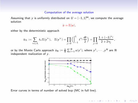
Computation of the average solution
Assuming that y is uniformly distributed on U = [!1,1]64, we compute the averagesolution
u = E(u),
either by the deterministic approach
u% :=#
""%
t"E(y"), E(y") =&
j>0
“
$ 1
!1t"j
dt
2
”
=&
j>0
1 +(!1)"j
2 +2"j,
or by the Monte Carlo approach uN := 1N
%Ni=1 u(y i), where y1, · · · ,yN are N
independent realization of y .
0 0.5 1 1.5 2 2.5 3 3.5
−14
−12
−10
−8
−6
−4
log10(#Λ)
log 10
(sup
rem
um a
vera
ge e
rror
)
Error curves in terms of number of solved bvp (MC in full line).

What I did not speak about
Use of Legendre polynomials instead of Taylor series : leads to approximation errorestimates in L2(U,dµ) with dµ the uniform measure on U.
Computation of the approximate Legendre coe"cients via Galerkin (projection)Adaptive strategy based on a-posteriori analysis.
Non-intrusive collocation methods : compute snapshots u(y) for y = y1,...,yN withN = #(%) and interpolate to obtain a polynomial
%""% c"y" . Di"culty : stability
(choice of yk) and adaptive search of %.
Space discretization : should be properly tuned (use di!erent resolution for each t")and injected in the final error analysis.
Our results can be used in the analysis of reduced basis methods.
Reconstruction of a sparse orthogonal series from random sampling : techniques fromCompressed Sensing (Sparse Fourier : Gilbert-Strauss-Tropp, Candes-Romberg-Tao,Rudelson-Vershynin. Sparse Legendre : Rauhut-Ward 2010).
Other models of parametric PDE’s currently studied of more general formF(u,y) = 0 : non-a"ne dependence of a in the variable y and other linear ornon-linear PDE’s.

Conclusion
Very high dimensional problems need very specific numerical treatment.
Theoretically challenging + many applications in engineering.
Key concepts and tools : sparsity, nonlinear approximation, tensorized decompositions,anisotropy, variable reduction, adaptivity...
Conclusion
Very high dimensional problems need very specific numerical treatment.
Theoretically challenging + many applications in engineering.
Key concepts and tools : sparsity, nonlinear approximation, tensorized decompositions,anisotropy, variable reduction, adaptivity...

Conclusion
Very high dimensional problems need very specific numerical treatment.
Theoretically challenging + many applications in engineering.
Key concepts and tools : sparsity, nonlinear approximation, tensorized decompositions,anisotropy, variable reduction, adaptivity...