high-frequency normal mode propagation in aluminum cylinders · high-frequency normal mode...

U.S. Department of the InteriorU.S. Geological Survey

Scientific Investigations Report 2009–5142

High-Frequency Normal Mode Propagation in Aluminum Cylinders

TIME, IN MICROSECONDS

100-mm-long cylinder


RELA

TIVE

AM

PLIT

UDE

–1,00015 30 45 60 75

0

1,000

2,000

P-wave crystalS-wave crystal

Shear wave

P100–1 P100–2

P200–1 P200–2P200–3

P100–3


By Myung W. Lee and William F. Waite


U.S. Department of the InteriorU.S. Geological Survey

U.S. Department of the InteriorKEN SALAZAR, Secretary

U.S. Geological SurveySuzette M. Kimball, Acting Director

U.S. Geological Survey, Reston, Virginia: 2009

For more information on the USGS—the Federal source for science about the Earth, its natural and living resources, natural hazards, and the environment, visit http://www.usgs.gov or call 1-888-ASK-USGS

For an overview of USGS information products, including maps, imagery, and publications, visit http://www.usgs.gov/pubprod

To order this and other USGS information products, visit http://store.usgs.gov

Any use of trade, product, or firm names is for descriptive purposes only and does not imply endorsement by the U.S. Government.

Although this report is in the public domain, permission must be secured from the individual copyright owners to reproduce any copyrighted materials contained within this report.

Suggested citation:Lee, M.W., and Waite, W.F., 2009, High-frequency normal mode propagation in aluminum cylinders: U.S. Geological Survey Scientific Investigations Report 2009–5142, 16 p.

iii

Contents

Abstract ...........................................................................................................................................................1Introduction.....................................................................................................................................................1Measuring Waveforms in Aluminum Cylinders ........................................................................................2Theory ..............................................................................................................................................................4

Wave Equation Solution .......................................................................................................................4Phase Velocity .......................................................................................................................................4Group Velocity .......................................................................................................................................5Normal Mode Amplitude .....................................................................................................................5Amplitude of P-Body Wave .................................................................................................................7Normal Mode and Body-Wave Amplitudes for P-Waves ..............................................................7S-Wave Amplitude ................................................................................................................................8

Discussion .......................................................................................................................................................8P-Wave Group Velocity ........................................................................................................................9S-Wave Group Velocity ........................................................................................................................9P-Wave Amplitudes ............................................................................................................................10S-Wave Amplitudes ............................................................................................................................11P-Wave Group Velocity: Dependence on Cylinder Radius ..........................................................12

Conclusions...................................................................................................................................................12Acknowledgments .......................................................................................................................................14References Cited..........................................................................................................................................14Appendix A. Low-Frequency and Large Diameter Approximation ..................................................16

Figures

1. Measurement equipment ............................................................................................................2 2. Waveforms for 35-mm-diameter and 100-mm and 200-mm nominal-length

aluminum cylinders surrounded by air at zero effective pressure .......................................3 3. Numerical derivation of theoretical phase velocities for a 35-mm-diameter

aluminum rod .................................................................................................................................6 4. Relation between wave number and frequency for fundamental and first-order

normal modes for a 35-mm-diameter aluminum cylinder ......................................................7 5. Calculated amplitude of the dispersive P-wave fundamental order normal mode

for a 35-mm-diameter, 100-mm-long aluminum cylinder ........................................................8 6. Group velocities for 35-mm-diameter aluminum cylinders....................................................9 7. Dispersive shear-wave normal mode analysis ......................................................................10 8. Predicted relative axial amplitudes for the P-body wave and fundamental and

first-order P-wave normal modes in a 35-mm-diameter, 200-mm-long aluminum cylinder ......................................................................................................................11

9. Predicted relative radial amplitudes of S-wave arrivals for a 35-mm-diameter, 200-mm-long aluminum cylinder ..............................................................................................11

10. Predicted relative radial amplitudes of the fundamental and first-order P-wave normal modes for a 35-mm-diameter, 100-mm-long aluminum cylinder ...........................12

iv

11. Normal mode dependence on cylinder radii..........................................................................13 12. Predicted relative amplitudes for the P-body wave and fundamental and

first-order normal modes in a 25.4-mm-diameter, 200-mm-long aluminum cylinder ......................................................................................................................14

Table

1. Velocities and dominant frequencies for normal mode arrivals in aluminum cylinders ......................................................................................................................3


By Myung W. Lee and William F. Waite

Abstract

Acoustic measurements made using compressional-wave (P-wave) and shear-wave (S-wave) transducers in aluminum cylinders reveal waveform features with high amplitudes and with velocities that depend on the feature’s dominant frequency. In a given waveform, high-frequency features generally arrive earlier than low-frequency features, typical for normal mode propagation. To analyze these waveforms, the elastic equation is solved in a cylindrical coordinate system for the high-frequency case in which the acoustic wavelength is small compared to the cylinder geometry, and the surrounding medium is air. Dispersive P- and S-wave normal mode propa-gations are predicted to exist, but owing to complex interfer-ence patterns inside a cylinder, the phase and group velocities are not smooth functions of frequency. To assess the normal mode group velocities and relative amplitudes, approximate dispersion relations are derived using Bessel functions. The utility of the normal mode theory and approximations from a theoretical and experimental standpoint are demonstrated by showing how the sequence of P- and S-wave normal mode arrivals can vary between samples of different size, and how fundamental normal modes can be mistaken for the faster, but significantly smaller amplitude, P- and S-body waves from which P- and S-wave speeds are calculated.

Introduction

Acoustic transmission through soil is strongly influenced by the nature of the intergranular contacts (Santamarina and others, 2001). Crystalline solids such as gas hydrate form-ing in the pore space of unconsolidated sediment can stiffen intergranular contacts or become load-bearing components of the sediment (Sloan and Koh, 2007), increasing the acous-tic velocity through the sediment (Guerin and others, 1999; Helgerud and others, 1999; Lee and Waite, 2008; Petersen and others, 2007; Yuan and others, 1999). The dependence of acoustic velocity on pore-space gas hydrate content depends on the transmitted wave’s propagation mode (Yun and others, 2006) and frequency (Bauer and others, 2005; Priest and oth-ers, 2005), the hydrate morphology and degree of saturation

within the pore space (Dvorkin and others, 2000; Kingston and others, 2008; Yun and others, 2005), as well as the porosity and lithology of the hydrate-bearing sediment itself (Guerin and Goldberg, 2005).

The gas hydrate and sediment test laboratory instrument (GHASTLI) (Winters and others, 2000) is one example of a laboratory system designed to investigate gas hydrate-bearing sediment, which can be found in marine and subpermafrost environments (Waite and others, 2004; Winters and others, 2004; Winters and others, 2007). GHASTLI is instrumented with compressional- and shear-wave transducers for pulse transmission through gas hydrate-bearing soil samples. Because it is designed for triaxial measurements of soil strength, GHASTLI requires cylindrical samples with lengths between 2 and 2.5 times their diameter (American Society for Testing and Materials, 2003). Correctly identifying observed compressional- and shear-waveform arrivals in these relatively long, narrow cylinders is complicated by the appearance of multiple high-amplitude features in the measured waveform (Waite and others, 2004, 2008).

To identify the observed arrivals and isolate geometric controls on the waveform shape from porous media effects, we carried out a series of measurements on aluminum cylinders of varying length and diameter. Based on the relation between the velocity, frequency, and amplitude of the waveform features, we can identify the high-amplitude features using a normal mode approach.

Normal mode solutions for layered Earth models have been investigated extensively, and many theories are avail-able (for example, Ewing and others, 1957; Brekhovskikh, 1960; Aki and Richards, 1980). Many wave propagation theories in thin cylinders at low frequencies, such as for bar waves, have also been developed and extensively analyzed by Kolsky (1963) and Graff (1975). However, these theories are not applicable to high-frequency measurements on relatively long, thin, cylindrical samples. Here we present a theory to calculate normal mode velocities and amplitudes and compare these results with values measured on aluminum cylinders. We derive the amplitude and dispersion relation for normal mode velocities using a cylindrical coordinate system, assuming a solid cylindrical body of infinite length surrounded by air, with a radius exceeding the acoustic wavelength.

2 High-Frequency Normal Mode Propagation in Aluminum Cylinders

Measuring Waveforms in Aluminum Cylinders

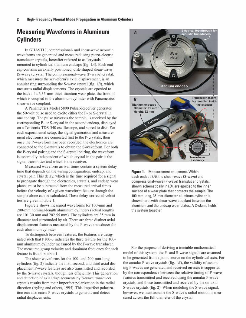
In GHASTLI, compressional- and shear-wave acoustic waveforms are generated and measured using piezo-electric transducer crystals, hereafter referred to as “crystals,” mounted in cylindrical titanium endcaps (fig. 1A). Each end-cap contains an axially positioned, disk-shaped shear-wave (S-wave) crystal. The compressional-wave (P-wave) crystal, which measures the waveform’s axial displacement, is an annular ring surrounding the S-wave crystal (fig. 1B), which measures radial displacements. The crystals are epoxied to the back of a 6.35-mm-thick titanium wear plate, the front of which is coupled to the aluminum cylinder with Panametrics shear-wave couplant.

A Panametrics Model 5800 Pulsar-Receiver generates the 50-volt pulse used to excite either the P- or S-crystal in one endcap. The pulse traverses the sample, is received by the corresponding P- or S-crystal in the second endcap, displayed on a Tektronix TDS-340 oscilloscope, and stored to disk. For each experimental setup, the signal generation and measure-ment electronics are connected first to the P-crystals; then once the P-waveform has been recorded, the electronics are connected to the S-crystals to obtain the S-waveform. For both the P-crystal pairing and the S-crystal pairing, the waveform is essentially independent of which crystal in the pair is the signal transmitter and which is the receiver.

Measured waveform arrival times contain a system delay time that depends on the wiring configuration, endcap, and crystal pair. This delay, which is the time required for a signal to propagate through the electronics, crystals, and endcap wear plates, must be subtracted from the measured arrival times before the velocity of a given waveform feature through the sample alone can be calculated. These delay-corrected veloci-ties are given in table 1.

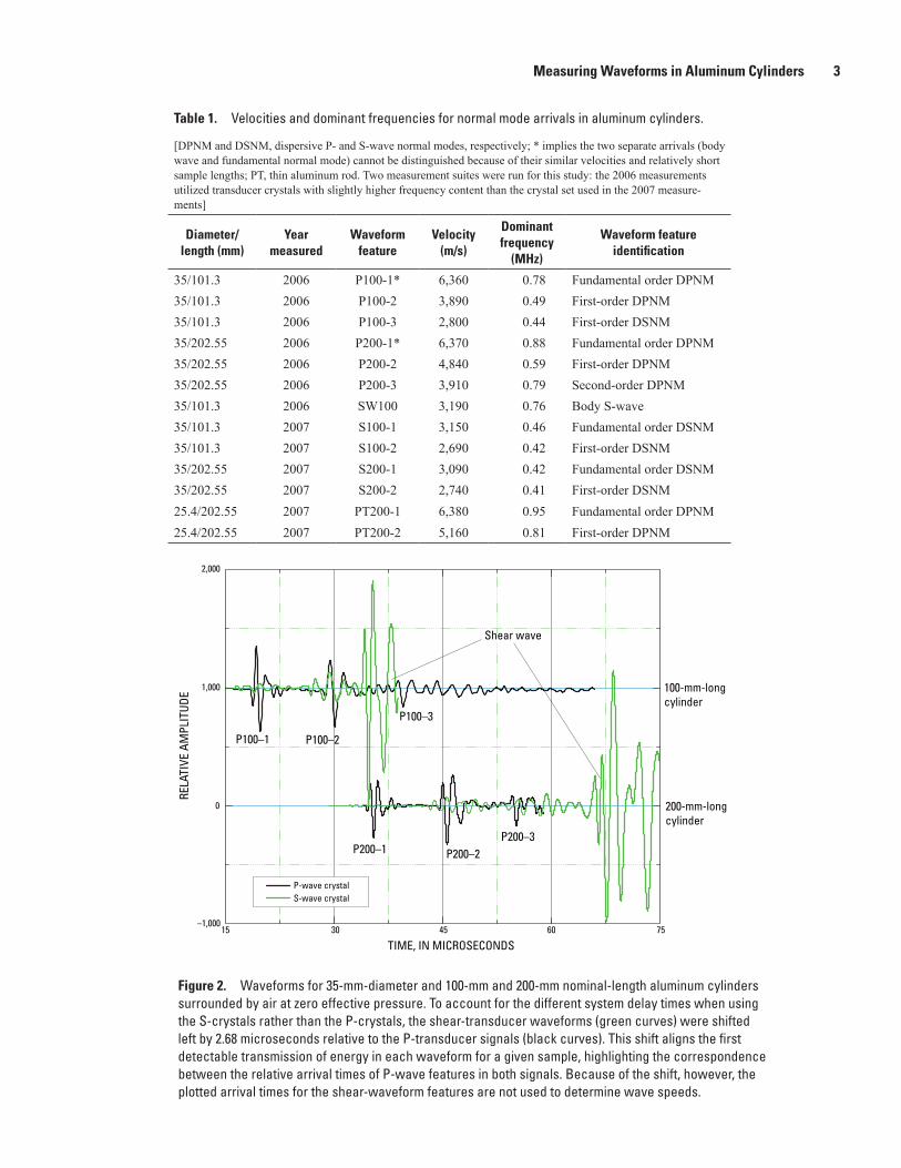
Figure 2 shows measured waveforms for 100-mm and 200-mm nominal-length aluminum cylinders (actual lengths are 101.30 mm and 202.55 mm). The cylinders are 35 mm in diameter and surrounded by air. There are three distinct axial displacement features measured by the P-wave transducer for each aluminum cylinder

To distinguish between features, the features are desig-nated such that P100-3 indicates the third feature for the 100-mm aluminum cylinder measured by the P-wave transducer. The measured group velocity and dominant frequency for each feature is listed in table 1.

The shear waveforms for the 100- and 200-mm-long cylinders (fig. 2) indicate the first, second, and third axial dis-placement P-wave features are also transmitted and recorded by the S-wave crystals, though less efficiently. This generation and detection of axial displacements by S-wave transducer crystals results from their imperfect polarization in the radial direction (Ayling and others, 1995). This imperfect polariza-tion can also cause P-wave crystals to generate and detect radial displacements.

Figure 1. Measurement equipment. Within each endcap (A), the shear-wave (S-wave) and compressional-wave (P-wave) transducer crystals, shown schematically in (B), are epoxied to the inner surface of a wear plate that contacts the sample. The 100-mm-long, 35-mm-diameter aluminum cylinder is shown here, with shear-wave couplant between the aluminum and the endcap wear plates. A C-clamp holds the system together.

For the purpose of deriving a tractable mathematical model of this system, the P- and S-wave signals are assumed to be generated from a point source on the cylindrical axis. For the annular P-wave crystals (fig. 1B), the validity of assum-ing P-waves are generated and received on-axis is supported by the correspondence between the relative timing of P-wave features transmitted and received using the annular P-wave crystals, and those transmitted and received by the on-axis S-wave crystals (fig. 2). When modeling the S-wave signal, however, we must assume the S-wave’s radial motion is mea-sured across the full diameter of the crystal.

A

B

Measuring Waveforms in Aluminum Cylinders 3

Table 1. Velocities and dominant frequencies for normal mode arrivals in aluminum cylinders.

[DPNM and DSNM, dispersive P- and S-wave normal modes, respectively; * implies the two separate arrivals (body wave and fundamental normal mode) cannot be distinguished because of their similar velocities and relatively short sample lengths; PT, thin aluminum rod. Two measurement suites were run for this study: the 2006 measurements utilized transducer crystals with slightly higher frequency content than the crystal set used in the 2007 measure-ments]

Diameter/length (mm)

Year measured

Waveformfeature

Velocity(m/s)

Dominantfrequency

(MHz)

Waveform featureidentification

35/101.3 2006 P100-1* 6,360 0.78 Fundamental order DPNM35/101.3 2006 P100-2 3,890 0.49 First-order DPNM35/101.3 2006 P100-3 2,800 0.44 First-order DSNM 35/202.55 2006 P200-1* 6,370 0.88 Fundamental order DPNM35/202.55 2006 P200-2 4,840 0.59 First-order DPNM35/202.55 2006 P200-3 3,910 0.79 Second-order DPNM35/101.3 2006 SW100 3,190 0.76 Body S-wave 35/101.3 2007 S100-1 3,150 0.46 Fundamental order DSNM35/101.3 2007 S100-2 2,690 0.42 First-order DSNM35/202.55 2007 S200-1 3,090 0.42 Fundamental order DSNM35/202.55 2007 S200-2 2,740 0.41 First-order DSNM25.4/202.55 2007 PT200-1 6,380 0.95 Fundamental order DPNM25.4/202.55 2007 PT200-2 5,160 0.81 First-order DPNM

Figure 2. Waveforms for 35-mm-diameter and 100-mm and 200-mm nominal-length aluminum cylinders surrounded by air at zero effective pressure. To account for the different system delay times when using the S-crystals rather than the P-crystals, the shear-transducer waveforms (green curves) were shifted left by 2.68 microseconds relative to the P-transducer signals (black curves). This shift aligns the first detectable transmission of energy in each waveform for a given sample, highlighting the correspondence between the relative arrival times of P-wave features in both signals. Because of the shift, however, the plotted arrival times for the shear-waveform features are not used to determine wave speeds.




RELA

TIVE

AM

PLIT

UDE

–1,00015 30 45 60 75

0

1,000

2,000

P-wave crystalS-wave crystal

Shear wave

P100–1 P100–2

P200–1 P200–2P200–3

P100–3


Theory

Identifying the waveform features listed in table 1 requires a theoretical relation between each normal mode’s dominant frequency and group velocity. We derive that rela-tion in three steps:1. Derive a solution of the wave propagation equation for

cylinders.

2. Derive the dispersion relation to obtain the normal mode phase velocity dependence on frequency.

3. Use the approximate phase velocity at high frequency to calculate the group velocity for each normal mode.As an independent check on the normal mode approach,

we also derive the relative amplitudes of the normal modes as well as of the P- and S-body waves.

Wave Equation Solution

Under the assumption of axial symmetry, differential equations for wave propagation within an infinitely long cylin-der can be written using a cylindrical coordinate system (r, θ, z) as (for example, Biot, 1952; Lee and Balch, 1982):

∂∂

+∂∂

+∂∂

=∂∂

2

2

2

2 2

2

2

1 1Φ Φ Φ Φr r r z t

∂∂

+∂∂

− +∂∂

=∂∂

2

2 2

2

2 2

2

2

1 1Ψ Ψ Ψ Ψ Ψr r r r z t

(1) , (1)

and Uz r rz =

∂∂

+∂∂

+Φ Ψ Ψ ,U

r zr =∂∂

−∂∂

Φ Ψ

where Φ and Ψ are scalar potentials for P- and S-waves, respectively; Ur and Uz are radial and axial displacement, respectively; and α, β, and t are P-wave velocity, S-wave velocity, and time, respectively. The formal solution of equa-tion 1 in the frequency domain can be written as follows when the P-wave source is located at the origin with the strength Vo, and the S-wave source is located at the origin with the strength So:

Φ = +∫ ∫− −AJ lr e dk V H lr e dkikzo

ikz0 0

2( ) ( )( )

Ψ = +∫ ∫− −BJ mr e dk S H mr e dkikzo

ikz1 1

2( ) ( )( ) , (2)

with

Φ Φ( ) ( ) =

−∞

∞

∫ t e dti t

l k k i k k= −⎛⎝⎜

⎞⎠⎟

> = − −⎛⎝⎜

⎞⎠⎟

<

2

22

1 2

22

2

/

/ sgnfor for /

m k k i k k= −⎛⎝⎜

⎞⎠⎟

> = − −⎛⎝⎜

⎞⎠⎟

<

2

22

1 2

22

2

/

/ sgn /for for

k c= /

where w is an angular frequency, c is the phase velocity, and Jn and Hn

( )2 are the order n Bessel function and order n Hankel function of the second kind, respectively. Note that uniformly expanding P- and S-wave source waves are assumed for the wave equation solution.

We use two boundary conditions in the solution of equa-tion 2: vanishing radial stress, prr= 0, and vanishing tangential stress, prz = 0 at the cylinder surface. Stresses are given by: p

r r zrr = − +∂∂

−∂∂ ∂

2

2

2

2

2

2Φ Φ Ψ

( )

, (3)

pr z zrz =

∂∂ ∂

− −∂∂

( )2 22 2

2

2

2

Φ Ψ Ψ

where l and m are the Lamé parameters.

Substituting boundary conditions into equation 3, the fol-lowing matrix equation can be derived: Q

a a

a a

A

B

S

S[ ] ≡

⎡

⎣⎢

⎤

⎦⎥

⎡

⎣⎢

⎤

⎦⎥ =

⎡

⎣⎢

⎤

⎦⎥

11 12

21 22

1

2

(4) with a k J la lJ la a11

2 2 20

212 2= − + ( ) ( ) ( ) /

a ik mJ ma

J ma

ao1212= −⎛

⎝⎜⎞⎠⎟

( )( )

a i k lJ la21 12= ( )

a k J ma22

2 2 212= − ( ) ( )

S V k H la V lH la ao o1

2 2 20

2 21

22 2= − − ( ) ( ) ( ) /( ) ( )

− −⎡⎣ ⎤⎦2 0

21

2ik S mH ma H mao ( ) ( ) /( )

S V iklH la S k H mao o2 12 2 2 2

122 2= − − − ( ) ( ) ( / ) ( )

Phase Velocity

The dispersion relation, meaning the normal mode phase velocity dependence on frequency, is given by requiring the determinant of equation 4 to be zero (Ewing and others, 1957). The determinant is given by a a a a11 22 12 21− :

Δ = − +4 2 2 41 0 1k lJ la mJ ma J ma a ( )[ ( ) ( ) / ]

(5) 2 2 2 2

12 2 2

02

12 2 2( ) ( )[( ) ( ) ( ) / ]k J ma k J la lJ la a− − +

in agreement with the equation shown by Graff (1975).Using the small argument approximation of the

Bessel functions in equation 5, we derive the low-frequency

Theory 5

dispersion relation in Appendix A, recovering the bar-wave velocity in a cylinder (Kolsky, 1963) and the Rayleigh surface-wave dispersion relation for large-diameter cylinders (White, 1965). The low-frequency corroboration with well-known wave behavior provides an important check on our theoreti-cal derivation. As described in Appendix A, however, for the high-frequency range of interest here, our observed waveform features (fig. 2) are neither the bar waves nor the extensional mode waveforms described by Kolsky (1963) and Graff (1975).

For the frequencies and length scales of interest here, the dispersion relation for the dispersive P-wave normal mode (DPNM) is derived by requiring the determinant given in equation 5 to be zero and the P-wave normal mode phase velocity to be greater than α. This restriction forces l and m to be real numbers. There is no simple analytic solution for finding the zeroes of equation 5. The dispersion relation can be numerically calculated, however. The phase velocity of a P-wave normal mode, Ca, is given by ∆ = 0 and can be written as: ( ) ( )[ ( )

( )]

( )[(

* *12

4 2

2

2

3

2

1 01

1

2

−=

−

C

C

l J la m J maJ ma

a

J maC

2 0

211

2− +) ( )

( )]

*

J lal J la

a

, (6)

where l C* /= −1 2 2 and m C* /= −1 2 2 . Allowable phase velocities are those for which the left and right sides of equation 6 are equal for a given phase velocity. From equation 6, the normal mode phase velocity depends on the acoustic-wave frequency, the P- and S-wave speed of the sample, and the sample’s geometry.

Figure 3 shows an example of calculating phase velocity using equation 6. Figure 3A shows phase velocities for the first three P-wave normal modes in a 35-mm-diameter aluminum cylinder at two different frequencies, calculated by determin-ing the locations of intersections of the left and right sides of equation 6. To develop the complete dependence of phase velocity on frequency, the process illustrated in figure 3A must be repeated for all frequencies in the range of interest. For the fundamental mode, the result is plotted in figure 3B.

The form of equation 6 is not practical for computing normal mode phase velocities. For the sake of simplicity at high frequencies, the measured dispersion relation can be approximated by setting either J la1 0( ) = or J la0 0( ) = in equation 6 for the P-wave normal modes. When using the approximate dispersion relation, the phase velocity (Ca) of a dispersive P-wave normal mode (DPNM) at high frequency is given by incorporating the high-frequency approximation of the Bessel functions, J la al al0 2 4( ) / ( ) cos( / )= − and J la al al1 2 3 4( ) / ( ) cos( / )= − (Watson, 1966), yielding:

C

a

a

=

−

2 2

2 2 2 2Λ , (7)

with Λ = +( / )3 4 n , if J la0 ( ) is set to zero, or Λ = +( / )5 4 n , if J la1( ) is set to zero. Results from both approximations are given in figure 3B. The exact fundamental mode phase velocities calculated from equation 6 (solid curve) are close to the approximate solution derived from setting J la0 0( ) = with n = 0 (dashed curve), and the approximation improves with increasing frequency. The approximation solu-tion using J la1 0( ) = with n = 0 (dotted curve) is much higher for all frequencies. The slope of the J la1 0( ) = curve more closely approximates the slope of the exact solution, which is an important characteristic for estimating the group velocity.

Group Velocity

Group velocities (G) are determined from the phase velocity (Ewing and others, 1957) according to: G

d

dkC k

dC

dk= = +

(8) Using the equation 7 approximation, the P-wave normal mode group velocity, Ga, is: G

d

dk a

= = − = −1 12 2

2 2

2

2

Λ ΛΠ

, (9) with Π = a / .

The dispersion relation for the DPNM requires both Bes-sel function approximations because the J la0 ( ) term in the determinant dominates the J la1( ) term in certain frequency ranges, the J la1( ) term dominates the J la0 ( ) term in other frequency ranges, and there are some frequency ranges for which neither term dominates.

S-wave normal mode phase velocities can be derived by requiring the normal mode phase velocity to be less than the P-wave velocity but greater than the S-wave velocity. This implies l is an imaginary number and m is a real number. Although l is imaginary, there exists a real solution for k. In contrast to the DPNM, the dispersion relation for dispersive shear-wave normal modes (DSNM) is better approximated using J

1(ma) = 0, and this approximation is appropriate for fre-

quencies greater than about 0.4 MHz for the 35-mm-diameter aluminum cylinder.

Normal Mode Amplitude

Amplitude relations provide an independent check on the normal mode technique for characterizing the waveform features shown in figure 2. Amplitude relations are also par-ticularly useful when differentiating between the fundamental normal modes and the body waves used to determine P- and S-wave speeds in materials. Normal mode amplitudes relative to each other can also be calculated from equations 2 and 4. With P- and S-wave sources at the origin, constants A and B in


equations 2 and 4 are given by: A (k) A = (S1a22 − S2a12 ) / ∆ ≡ P

∆(k) (10) A (k)

B = (−S a + S a ) / ≡ S1 21 2 11 ∆

∆(k)

In the following amplitude analysis, only P-waves are considered. Substituting from equations 4 and 5 into equation 10: A (k) = −V 2 (2k2 2− 2 )2 J (ma)H (2)(la)

P o 1 0

− V 2 22 2 2

o 1 ( k 2 − 2 )lJ11(ma)H (2)1 (la) / a

− V 2 2 4 2

o 4k lH1 (la)[mJ0 (ma) − J1(ma) / a] (11)

− 2iS02 2k(2k2 2− 2 )J1(ma)[mH 2

0 (ma)

− H 21 (ma) / a]

+ 2iS 22 ( 2

0 k 2k 2−− 2 )H1(ma)[mJo(ma)

− J1(ma) / a]

Substituting A into the integral equation shown in equa-tion 2, the potential for the P-wave solution is given by the following equation (for example, Pekeris, 1948; Ewing and others, 1957; Båth, 1968) in the lower half of the complex k-plane: ∞Φ(k) = ∫

∞A(k)J −ikz (2) −ikz

0 (lr)e dk + Vo H0 (lr)e dk−∞ ∫−∞

= ∫ [A(k) J (llr) + V H (2) (lr)]e −ikzdk − 2 i∑ RP

0 o 0 n (12)

Branch cut

= ΦB + ΦDPNM

where Branch cut is a branch cut integration around the branch points k P

= / and k = / ; Rn is the residue of inte-gration for a dispersive P-wave normal mode; ΦB and ΦDPNM are the P-wave potentials for a body wave and a dispersive P-wave normal mode, respectively.

The dispersive P-wave normal mode amplitude can be calculated by substituting the wave number, k, of interest into equation 12. The DPNM solution from the P-wave source is given by:

Figure 3. Numerical derivation of theoretical phase velocities for a 35-mm-diameter aluminum rod with an assumed P-wave velocity, α, of 6,380 m/s and S-wave velocity, β, of 3,180 m/s. A, For 0.585 and 0.589 MHz, the fundamental and first- and second-order normal mode phase velocities relative to a (radius of a cylinder) are, respectively, given by the first, second, and third intersections between the left and right hand sides of equation 6. B, Phase velocities of the fundamental order P-wave normal mode calculated from equation 6 are compared with those calculated from the approximate dispersion relations with n = 0.

A B

NORMALIZED PHASE VELOCITY, Cα /α

NO

RMA

LIZE

D P

HA

SE V

ELO

CITY

, Cα /α

FREQUENCY, IN HERTZ

RIG

HT

AN

D L

EFT

SID

E O

F EQ

UAT

ION

6

1.00–4 0.8

0.9

1.0

1.1

1.2

–2

0

2

4

6

1.25 1.50 1.75 4×105 6×105 8×105 1×106

Phase velocity for fundamental order

Calculated for P200–2

Exact equation

Left side of equation 6Right side of equation 6 for f = 0.585 mHzRight side of equation 6 for f = 0.589 mHz

Fundamental order

First order

Second order

Approximation using J1(la) = 0

Approximation using J0(la) = 0

Theory 7

ΦΔDPNM

Pikz

k solution of equation

iA k J lr e

k=

−∂ ∂

−

=

2 06

( ) ( )

/] , (13)

where ∆ is given in equation 5 and AP is given in equation 11.

Amplitude of P-Body Wave

The branch cut integrations shown in equation 12 yield body-wave motions inside the solid. The branch cut integra-tion can be evaluated using the steepest descent method (for example, Morse and Feshbach, 1953; Båth, 1968; Greenfield, 1978) if the observation point is in the far field, meaning the wave travels a distance much longer than its wavelength. Using Hankel functions, equation 12 can be written as:

ΦBikz

oikzA k J lr e dk V H lr e dk

A k

( ) ( ) ( ) ( )

[ (

( ) = +

=

−∞

∞ − −

−∞

∞

∫ ∫

∫

0 02

1

2)) ( ) ( ( ) ) ( )] .( ) ( )H lr A k V H lr e dkikz

01

0 022+ + −

The integration using the steepest descent method yields:

ΦBo

i RiA k R

R

iV e

R≈ +

−2 2( cos )cos( / ) / ‘

(14)

where k = / , = −tan ( / )1 r z and R z r= +2 2 .

The displacements can be written as:

Ur

i rA k R

R

rV e

RrB o

i R

=∂∂

≈−

+−Φ 2 2

2 2

( cos )sin( / ) /

(15)

Uz

i zA k R

R

zV e

RzB o

i R

=∂∂

≈−

+−Φ 2 2

2 2

( cos )sin( / )

./

The far-field solution shown in equation 14 requires the Bessel and Hankel function argument to be large: lr >> 1. However, the geometry of our measurement does not satisfy the condi-tion because the cylinder radius, α, and observation point radius, r, are both small. We can therefore only approximate the body-wave amplitude, and we do so by assuming the uniformly expanding source waveform can be calculated by making a and r large. In other words, we ignore the first term of equation 14, which yields the reflections from the cylinder boundaries. From equation 14, the body-wave amplitude for the P-wave can be approximated by:

Ur ≈ 0

UV e

zz

i z

≈−2 0

/

and (16)

Normal Mode and Body-Wave Amplitudes for P-Waves

The discontinuous phase velocity that complicates the group velocity calculation is also a problem when using

equation 13 to calculate normal mode amplitudes. Figure 4 shows the wave number calculated using equation 6 for the fundamental and first-order DPNM over the measured range of dominant frequencies. Like the phase velocities shown in figure 3B, the relation between wave number and frequency is discontinuous. Using the same technique employed for figure 3B, the discontinuous exact solution can be approxi-mated by setting J la0 0( ) .=

The approximation works well for the fundamental and first-order modes at high frequencies. Although the general trend of the approximation follows the exact relation, the approximate solution becomes less accurate with decreasing frequency. Numerical analysis indicates the approximation becomes worse as the order of the normal mode increases.

Equation 13 requires the phase velocity rather than the group velocity to compute normal mode amplitude. Based on figure 4, we assume the approximate phase velocities derived from J la0 0( ) = with n = 0 and n = 1 are appropriate to quali-tatively analyze amplitudes of the fundamental and first-order DPNM. A second option for approximating the phase velocity is to set J

1(la) = 0, which, as discussed previously, and shown

Figure 4. Relation between wave number and frequency for fundamental and first-order normal modes for a 35-mm-diameter aluminum cylinder. Approximate relation using J0(la) = 0 with n = 0 and 1 are also shown. The approximations improve with increasing frequency and decreasing order of the normal mode.

WAVE NUMBER, RADIANS PER METER

ANGU

LAR

FREQ

UEN

CY, R

ADIA

NS

PER

SECO

ND

3 ×106 4 ×106 5 ×106 6 ×106 7 ×1063 ×106

4 ×106

5 ×106

6 ×106

7 ×106

Fundamental mode from exact equationFirst order from exact equation

Approximation using JO(la) = 0 with n=0

Approximation using JO(la) = 0 with n=1


in figure 3B, appears to more accurately fit the slope of the exact phase velocity solution (equation 6). Because this slope is important in calculating the group velocity in equation 8, and since it is the group velocity, not the phase velocity, that is easily estimated from the measured waveform, using J

1(la)

= 0 for the approximation rather than J la0 0( ) = is tempting. As demonstrated in figure 5, however, this approximation does not reflect the exact solution behavior for normal mode amplitudes.

Figure 5 shows calculated amplitudes of the fundamental mode for a 100-mm-long, 35-mm-diameter aluminum cylinder using the exact solution, the J la0 0( ) = , and the J

1(la) = 0

approximations. The exact solution agrees well with the J la0 0( ) = for frequencies away from the spectral holes at the phase-velocity discontinuities, but is generally at least an order of magnitude below the J

1(la) = 0 approximation. There-

fore, all P-wave normal mode amplitudes in this paper are

computed using J la0 0( ) .= For comparison, the body-wave amplitude shown in figure 5 is calculated from equation 16. Figure 5 indicates the approximate normal mode amplitudes are larger than the body-wave amplitude for all frequency ranges. The amplitudes calculated from the exact solution are also larger than the body wave except near the spectral holes. This finding suggests body waves will likely be difficult to detect unless they arrive well in advance of the fundamental mode.

S-Wave Amplitude

As mentioned previously, to analyze the shear-wave normal mode, we consider phase velocities greater than b and less than a. Shear-wave propagation can be calculated using the same equations used for the P-wave propagation with the following constant: B k

B kV k ik l J la H la

J la H

So( )

( )( ) [ ( ) ( )

( )

( )

(

≡ = −

−Δ

2 22 2 2 2 21 0

2

0 1

22

2 4 21 1

2

2 2 41

4

4

)

( )

( )] /

( ( ) ( ) / ) /

(

la

V ik l J la H la a

S k lJ

o

o

Δ

Δ+

− {

lla mH ma H ma a

k J la H ma

)[ ( ) ( ) / ]

( ) ( ) ( ) /

( ) ( )

( )

02

12

2 2 2 20 1

22

− +

− } Δ

(17)

Using a similar argument for the P-wave, the S-body wave amplitude is approximated as: U

i S e

zro

i z

≈ −−2

/

(18)

Uz ≈ 0 .

Discussion

To demonstrate the utility of the normal mode approach, we identify waveform features by comparing their group velocities and dominant frequencies (see table 1) to theoretical values for each normal mode. Body waves are identified on the basis of the arrival time and amplitude comparisons to the fundamental mode amplitudes. We begin with considering waveforms from cylinders of different length, but identical radii. Later in this report, we consider waveforms from cylinders of identical length but different radii.

Figure 5. Calculated amplitude of the dispersive P-wave fundamental order normal mode (fundamental order DPNM) for a 35-mm-diameter, 100-mm-long aluminum cylinder. Between the spectral holes caused by discontinuities in the phase velocity near 0.65, 0.75, and 0.86 MHz. Setting J0(la) = 0 in equation 13 provides a close approximation to the exact amplitude calculation.

RELA

TIVE

AXI

AL D

ISPL

ACEM

ENT

FREQUENCY, IN HERTZ

6 ×105103

104

105

106

107

7 ×105 8 ×105 9 ×105

Body wave

Fundamental order DPNM with J0(la) = 0

Fundamental order DPNM with J1(la) = 0

Fundamental order DPNM with exact dispersion relation

Discussion 9

P-Wave Group Velocity

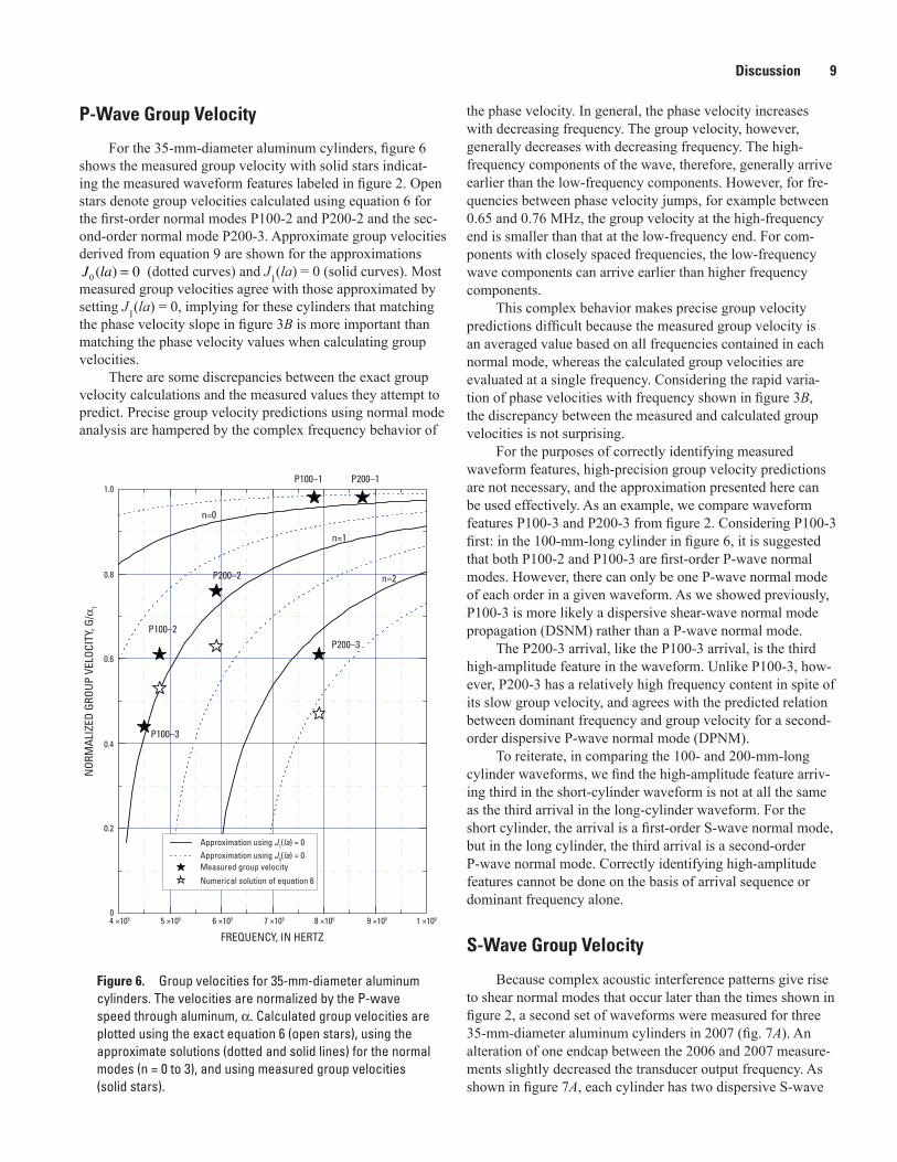
For the 35-mm-diameter aluminum cylinders, figure 6 shows the measured group velocity with solid stars indicat-ing the measured waveform features labeled in figure 2. Open stars denote group velocities calculated using equation 6 for the first-order normal modes P100-2 and P200-2 and the sec-ond-order normal mode P200-3. Approximate group velocities derived from equation 9 are shown for the approximations J la0 0( ) = (dotted curves) and J

1(la) = 0 (solid curves). Most

measured group velocities agree with those approximated by setting J

1(la) = 0, implying for these cylinders that matching

the phase velocity slope in figure 3B is more important than matching the phase velocity values when calculating group velocities.

There are some discrepancies between the exact group velocity calculations and the measured values they attempt to predict. Precise group velocity predictions using normal mode analysis are hampered by the complex frequency behavior of

the phase velocity. In general, the phase velocity increases with decreasing frequency. The group velocity, however, generally decreases with decreasing frequency. The high-frequency components of the wave, therefore, generally arrive earlier than the low-frequency components. However, for fre-quencies between phase velocity jumps, for example between 0.65 and 0.76 MHz, the group velocity at the high-frequency end is smaller than that at the low-frequency end. For com-ponents with closely spaced frequencies, the low-frequency wave components can arrive earlier than higher frequency components.

This complex behavior makes precise group velocity predictions difficult because the measured group velocity is an averaged value based on all frequencies contained in each normal mode, whereas the calculated group velocities are evaluated at a single frequency. Considering the rapid varia-tion of phase velocities with frequency shown in figure 3B, the discrepancy between the measured and calculated group velocities is not surprising.

For the purposes of correctly identifying measured waveform features, high-precision group velocity predictions are not necessary, and the approximation presented here can be used effectively. As an example, we compare waveform features P100-3 and P200-3 from figure 2. Considering P100-3 first: in the 100-mm-long cylinder in figure 6, it is suggested that both P100-2 and P100-3 are first-order P-wave normal modes. However, there can only be one P-wave normal mode of each order in a given waveform. As we showed previously, P100-3 is more likely a dispersive shear-wave normal mode propagation (DSNM) rather than a P-wave normal mode.

The P200-3 arrival, like the P100-3 arrival, is the third high-amplitude feature in the waveform. Unlike P100-3, how-ever, P200-3 has a relatively high frequency content in spite of its slow group velocity, and agrees with the predicted relation between dominant frequency and group velocity for a second-order dispersive P-wave normal mode (DPNM).

To reiterate, in comparing the 100- and 200-mm-long cylinder waveforms, we find the high-amplitude feature arriv-ing third in the short-cylinder waveform is not at all the same as the third arrival in the long-cylinder waveform. For the short cylinder, the arrival is a first-order S-wave normal mode, but in the long cylinder, the third arrival is a second-order P-wave normal mode. Correctly identifying high-amplitude features cannot be done on the basis of arrival sequence or dominant frequency alone.

S-Wave Group Velocity

Because complex acoustic interference patterns give rise to shear normal modes that occur later than the times shown in figure 2, a second set of waveforms were measured for three 35-mm-diameter aluminum cylinders in 2007 (fig. 7A). An alteration of one endcap between the 2006 and 2007 measure-ments slightly decreased the transducer output frequency. As shown in figure 7A, each cylinder has two dispersive S-wave

Figure 6. Group velocities for 35-mm-diameter aluminum cylinders. The velocities are normalized by the P-wave speed through aluminum, α. Calculated group velocities are plotted using the exact equation 6 (open stars), using the approximate solutions (dotted and solid lines) for the normal modes (n = 0 to 3), and using measured group velocities (solid stars).

NOR

MAL

IZED

GRO

UP V

ELOC

ITY,

G/α

1

FREQUENCY, IN HERTZ4 ×105 5 ×105 6 ×105 7 ×105 8 ×105 9 ×105 1 ×1060

0.2

0.4

0.6

0.8

1.0

Measured group velocity

P100–3

P100–2

P100–1 P200–1

P200–2

P200–3

n=0

n=1

n=2

Numerical solution of equation 6

Approximation using J1(la) = 0Approximation using J0(la) = 0


normal modes (DSNM), identified as S100-1, S100-2, S150-1, S150-2, S200-1, and S200-2. The group velocities of the fundamental and first-order DSNM for 100- and 200-mm-long aluminum cylinders are shown in figure 7B, along with wave-form feature P100-3 from figures 2 and 6. The group velocities of P100-3 and S100-2 follow the first-order DSNM curve. Therefore, the P100-3 shown in figure 2 is probably the axial component of the first-order DSNM propagation, designated as S100-2 in figure 7A.

P-Wave Amplitudes

Here we qualitatively compare amplitudes of waveform features in the frequency domain. The body-wave and DPNM amplitudes from a P-wave source in a 200-mm-long aluminum cylinder with a 35-mm diameter are plotted in figure 8. The shaded regions cover the dominant frequency ranges measured for the fundamental and first-order normal modes, and are centered on the predicted relative amplitude for that phase. Figure 8 indicates the fundamental and first-order normal modes have similar amplitudes, with the fundamental mode

having a slightly higher amplitude than the first-order mode, in agreement with the measured waveforms shown in figure 2. The calculated amplitude of the body wave is much smaller than either normal mode.

Because the arrival times of the fundamental order DPNM are so close to those of the first arrival P-body wave for the 100- and 200-mm-long aluminum cylinders, the body wave is indistinguishable from the fundamental normal mode. Two consequences for these cylinders are (1) using the fundamental order DPNM as a proxy for the body wave in determining the P-wave speed in aluminum underpredicts the P-wave speed of 6,380 m/s by only 0.3 percent, and (2) the measured fundamental order DPNM is a mixture of normal mode and body-wave arrivals. The body-wave amplitude is much smaller than that of the fundamental order DPNM for these cylinders, but as the cylinder length decreases, the body-wave amplitude varies as 1/(cylinder length), whereas the normal mode amplitude is independent of the cylinder length. Thus, the body wave becomes more distinct as the normal mode interference diminishes with decreasing cylinder length.

Figure 7. Dispersive shear-wave normal mode analysis. A, Shear-wave waveforms for 35-mm-diameter aluminum cylinders (AL) of nominal length 100, 150 and 200 mm, all measured in 2007. S100-1, S150-1, and S200-1 are fundamental order dispersive S-wave normal modes (DSNM) observed for 100-, 150- and 200-mm-diameter cylinders, respectively. Similarly, S100-2, S150-2, and S200-2 are the first-order DSNM. B, Measured and calculated group velocities for S100-1, S100-2, S200-2, and P100-3. P100-3 is likely the axial component of the first-order shear normal mode. Group velocities are normalized to the shear-wave speed in aluminum, β.

NOR

MAL

IZED

GRO

UP V

ELOC

ITY,

Gβ/β

RELA

TIVE

AM

PLIT

UDE

FREQUENCY, IN HERTZ

From approximation J1(ma) = 0From S–transducerFrom P–transducer


15 30 45 60 75 90–3,000

3,000

6,000

9,000

0200-mm AL

150-mm AL

S100–1

S100–2

S100–2

S200–1S100–1

S200–2

n = 0

n = 1S150–2

S150–1

First–S arrival

S200–1

S200–2

100-mm AL

2 ×105 4 ×105 6 ×10500

0.2

0.4

0.6

0.8

1.0A B

Discussion 11

S-Wave Amplitudes

Figure 9 shows the calculated radial amplitudes for vari-ous arrivals for a 200-mm-long, 35-mm-diameter cylinder from an S-wave source. The shaded region spans the domi-nant frequencies of the measured first-order and fundamental modes. In agreement with figure 7A, the radial displacements of the fundamental and first-order DSNM are similar. Because normal mode amplitude is independent of the cylinder length, the amplitude relations between the fundamental and first-order DSNM remains similar for all three aluminum cylinders. The measured amplitude relation between the S-body wave and fundamental order DSNM for the 200-mm-long aluminum cylinder also agrees with the calculated relation.

The shear crystal traces in figure 2 show the radial dis-placement of the P-wave normal modes P100-1 and P100-2, indicating the radial amplitude of P100-2 is larger than that of P100-1. Figure 10 shows the calculated radial displace-ment for fundamental and first-order DPNM, indicating the

radial displacement of P100-2 is larger than that of P100-1, in qualitative agreement with the observed amplitude variation. Because the P-wave normal mode amplitude is independent of the length of the aluminum cylinder, the calculated and measured radial displacements of P200-2 are also larger than those of P200-1.

As was the case for P-waves, arrival times of the funda-mental order DSNM and S-body wave are close. The 100-1, S150-1, and S200-1 waveforms in figure 7A are therefore mix-tures of the fundamental normal mode and the body wave. In the 200-mm-long cylinder, however, a small amplitude event with high-frequency content arrives earlier than S200-1 and is separated from the fundamental order DSNM. We interpret this earlier arrival as the first arrival S-body wave. This wave-form demonstrates how the nearly identical body-wave and fundamental DSNM-wave speeds mean the body wave can only separate from the fundamental mode in long cylinders. For the 200-mm-long cylinder, interpreting the largest feature, S200-1, as the body wave would underpredict the shear-wave

Figure 8. Predicted relative axial amplitudes for the P-body wave and fundamental and first-order P-wave normal modes in a 35-mm-diameter, 200-mm-long aluminum cylinder. Fundamental and first-order normal mode amplitudes are similar, and both are much larger than the body-wave amplitude.

Figure 9. Predicted relative radial amplitudes of S-wave arrivals for a 35-mm-diameter, 200-mm-long aluminum cylinder. The fundamental and first-order normal modes have comparable amplitudes, and both are significantly larger than the S-body wave, in agreement with figure 7A.

RELA

TIVE

AXI

AL A

MPL

ITUD

E

First-order DPNM with J1(la) = 0

Body wave

Dominant frequency of fundamental order

Dominant frequency of first order

r = 0 cm

Fundamental order DPNM with JO(la) = 0

4 ×105103

104

105

106

107

5 ×105 6 ×105 7 ×105 8 ×105

FREQUENCY, IN HERTZ

RELA

TIVE

RAD

IAL

DISP

LACE

MEN

TFirst-order DSNM using J1(ma) = 0

Body wave

Dominant frequencies of fundamental and first-order DSNM

Fundamental order DSNM with J1(ma) = 0

FREQUENCY, IN HERTZ2 ×105 4 ×105 6 ×105 8 ×105 1 ×106

103

104

105

106


Figure 10. Predicted relative radial amplitudes of the fundamental and first-order P-wave normal modes for a 35-mm-diameter, 100-mm-long aluminum cylinder. In agreement with the shear-wave traces in figure 2, the first-order normal mode amplitudes are greater than the fundamental mode amplitudes.

speed of 3,180 m/s by 1 percent. As shown in figure 2, the high wave speed of P-waves relative to S-waves, and the close agreement between the P-body wave and fundamental normal mode, mean the P-body wave does not separate from the fun-damental mode, even in the 200-mm-long cylinder.

P-Wave Group Velocity: Dependence on Cylinder Radius

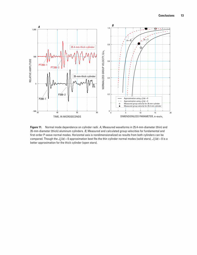
Figure 11A compares measured waveforms in 35- and 25.4-mm-diameter, 200-mm nominal-length aluminum cylinders. The waveforms, generated and measured with the P-wave crystals, contain two notable differences in the thin cylinder: (1) the first-order DPNM arrives more quickly than in the thick cylinder, and (2) the first-order DPNM is at least twice the amplitude of the fundamental mode.

The normal mode group velocities, compared with theoretical predictions in figure 11B, further exemplify the

RELA

TIVE

RAD

IAL

DISP

LACE

MEN

T

First-order DPNM

Dominant frequency of fundamental order


Fundamental order DPNM

FREQUENCY, IN HERTZ4 ×105 5 ×105 6 ×105 7 ×105 8 ×105

102

103

104

105

106

107 control that sample geometry exerts on waveform structure. The horizontal axis in 11B has been nondimensionalized so results from cylinders of different radii can be compared. The normal mode approximations agree with the measured results, but it is the J

0(la) = 0 approximation that works for the

25.4-mm-diameter cylinder, whereas the J1(la) = 0 approxima-

tion is more appropriate for the 35-mm-diameter cylinder. As predicted by the normal mode approach, the complex internal reflection patterns that create these normal modes produce a much higher first-order normal mode amplitude relative to the fundamental mode in the thin cylinder (fig. 12), but nearly equal amplitudes in the thick cylinder (fig. 8).

Conclusions

Laboratory measured elastic waveforms in cylinders can contain large amplitude waveform features that can make it difficult to identify the nature of each arrival. Sample geom-etry influences the group velocity and amplitude of each feature differently, meaning their arrival sequence and relative amplitudes within a waveform can all differ in samples of dif-ferent size. These waveform features behave as normal mode propagations, which we identify and characterize using a wave propagation solution in a cylindrical coordinate system.

The primary challenge in correctly identifying the observed normal modes is coping with the discontinuous frequency dependence of their phase velocities. Identifying normal modes via amplitude and group velocity predictions can be accomplished by using Bessel functions to approximate the phase-velocity dependence on frequency. The accuracy of these approximations improves with increasing frequency as the situation more closely resembles a small wavelength signal traveling along the axis of a large, long cylinder.

Two key findings from this study are:1. P- and S-wave crystals each produce a combination

of P- and S-wave normal modes. A waveform can therefore contain both P- and S-wave normal modes, with their arrival order depending on the sample geometry in a manner that is difficult to predict from a visual inspection of the waveform. These arriv-als can be identified by analyzing amplitude and group velocities in the context of normal mode wave propagation.

2. Body waves, which travel at the P- and S-wave speeds generally sought after in acoustic measure-ments, can be obscured by the relatively higher amplitude fundamental normal modes. When the cylinder is long, or the wave speed is low, the body wave can measurably separate from the fundamental mode. In these cases, the more easily observed fun-damental mode may be mistaken for the body wave, leading to an underestimate of the P- or S-wave speed.

Conclusions 13

Figure 11. Normal mode dependence on cylinder radii. A, Measured waveforms in 25.4-mm-diameter (thin) and 35-mm-diameter (thick) aluminum cylinders. B, Measured and calculated group velocities for fundamental and first-order P-wave normal modes. Horizontal axis is nondimensionalized so results from both cylinders can be compared. Though the J0(la) = 0 approximation best fits the thin cylinder normal modes (solid stars), J1(la) = 0 is a better approximation for the thick cylinder (open stars).

A B

TIME, IN MICROSECONDS DIMENSIONLESS PARAMETER, π=aω/α1

RELA

TIVE

AM

PLIT

UDE

NOR

MAL

IZED

GRO

UP V

ELOC

ITY,

G/α

1

30–500

0

500

1,000

40 50 60 00

0.2

0.4

0.6

0.8

1.0

5 10 15 20

Measured group velocity for 35-mm cylinderMeasured group velocity for 25.4-mm cylinder

Approximation using J1(la) = 0Approximation using J0(la) = 0

P200–1

PT200–1PT200–2

P200–2

n = 0 n = 1

35-mm-thick cylinder

25.4-mm-thick cylinder


Acknowledgments

This work was supported by the Gas Hydrate Project within the U.S. Geological Survey’s Energy and Coastal and Marine Geology Programs. We thank Peter M. Bratton for his assistance in measuring acoustic waveforms.

References Cited

Aki, Keith, and Richards, P.G., 1980, Quantitative seismology—theory and methods: New York, Freeman, 932 p.

American Society for Testing and Materials, 2003, D 2850-03a standard test method for unconsolidated- undrained triaxial compression test on cohesive solids, in Annual Book of ASTM Standards, edited: ASTM Interna-tional, p. 1–6.

Ayling, M.R., Meredith, P.G., and Murrell, S.A.F., 1995, Microcracking during triaxial deformation of porous rocks monitored by changes in rock physical properties, Part I, Elastic-wave propagation measurements on dry rocks: Tectonophysics, v. 245, p. 205–221.

Båth, Markus, 1968, Developments in solid earth geophysics: New York, Elsevier, 415 p.

Bauer, K.C., Haberland, R.G., Pratt, F., Hou, B., Medioli, E., and Weber, M.H., 2005, Ray-based cross-well tomography for P-wave velocity, anisotropy, and attenuation structure around the JAPEX/JNOC/GSC and others Mallik 5L-38 gas hydrate production research well, in Dallimore, S.R., and Collett, T.S., eds., Scientific results from the Mallik 2002 gas hydrate production research well program, Mackenzie Delta, Northwest Territories, Canada: Geological Survey of Canada Bulletin 585, 21 p.

Biot, M. 1952, Propagation of elastic waves in a cylindrical bore containing a fluid: Journal of Applied Physics, v. 23, p. 997–1,009.

Brekhovskikh, L.M., 1960, Waves in layered media: New York, Academic Press, 559 p.

Dvorkin, Jack, Helgerud, M.B., Waite, W.F., Kirby, S.H, and Nur, A., 2000, Introduction to physical properties and elasticity models in natural gas hydrate, in Max, M.D., ed., Oceanic and permafrost environments: Boston, Kluwer Academic Publishers, p. 245–260.

Ewing, W.M., Jardetzky, W.S., and Press, F., 1957, Elastic waves in layered media: New York, McGraw-Hill, 380 p.

Graff, K.F.,1975, Wave motion in elastic solids: New York, Dover, 649 p.

RELA

TIVE

AXI

AL D

ISPL

ACEM

ENT

FREQUENCY, IN HERTZ6 ×105

103

104

105

106

107

7 ×105 8 ×105 9 ×105 1 ×106

Body wave

Dominant frequency of fundamental mode


Fundamental order DPNM with J0(la) = 0First-order DPNM with J0(la) = 0

Figure 12. Predicted relative amplitudes for the P-body wave and fundamental and first-order normal modes in a 25.4-mm-diameter, 200-mm-long aluminum cylinder. Both normal mode amplitudes are significantly larger than the P-body-wave amplitude. Unlike the 35-mm-diameter aluminum cylinder results (fig. 8), the first-order normal mode amplitude is larger than that of the fundamental mode. This prediction is in agreement with the results shown in figure 11.

References Cited 15

Greenfield, R.J., 1978, Seismic radiation from a point source on the surface of a cylindrical cavity: Geophysics, 43, p. 1,071–1,982.

Guerin, Giles, and Goldberg, D., 2005, Modeling of acous-tic wave dissipation in gas hydrate-bearing sediments: Geochemistry Geophysics Geosystems, v. 6, Q07010, doi:10.1029/2005GC000918, 16 p.

Guerin, Giles, Goldberg, D., and Meltser, A., 1999, Characterization of in situ elastic properties of gas hydrate-bearing sediments on the Blake Ridge: Journal of Geophysical Research, v. 104, p. 17,781–17,795.

Helgerud, M.B., Dvorkin, J., Nur, A., Sakai, A., and Collett, T., 1999, Elastic-wave velocity in marine sediments with gas hydrates: Effective medium modeling: Geophysical Research Letters, v. 26, p. 2,021–2,024.

Kingston, Emily, Clayton, C., and Priest, J., 2008, Gas hydrate growth morphologies and their effect on the stiffness and damping of a hydrate bearing sand: Presented at Vancouver, Canada, 6th International Conference on Gas Hydrates, July 6–10, 2008, 8 p.

Kolsky, Herbert, 1963, Stress waves in solids: New York, Dover, 213 p.

Lee, M.W., and Balch, A.H., 1982, Theoretical seismic wave propagation from a fluid-filled borehole: Geophysics, v. 47, p. 1,308–1,314.

Lee, M.W., and Waite, W.F., 2008, Estimating pore-space gas hydrate saturations from well-log acoustic data: Geochemistry Geophysics Geosystems, v. 9, Q07008, doi:10.1029/2008GC002081, 8 p.

Morse, P.M., and Feshbach, H., 1953, Methods of theoretical physics, Part I: New York, McGraw-Hill, 988 p.

Pekeris, C.L., 1948, Theory of propagation of explosive sound in shallow water: Geological Society of America Memoir 27, 117 p.

Petersen, C.J., Papenberg, C., and Klaeschen, D., 2007, Local seismic quantification of gas hydrates and BSR character-ization from multi-frequency OBS data at northern Hydrate Ridge: Earth and Planetary Science Letters, v. 255, p. 414–431.

Priest, J.A., Best, A., and Clayton, C.R., 2005, A laboratory investigation into the seismic velocities of methane gas hydrate-bearing sand: Journal of Geophysical Research, 110, B04102, doi:10.1029/2004JB003259.

Santamarina, J.C., Klein, K.A., and Fam, M.A., 2001, Soils and waves: Particulate materials behavior, characterization and process monitoring: New York, Wiley, 488 p.

Sloan, E.D., and Koh, C.A., 2007, Clathrate hydrates of natural gases, 3rd ed: Boca Raton, CRC Press, 721 p.

Waite, W.F., Kneafsey, T.J., Winters, W.J., and Mason, D.H., 2008, Physical property changes in hydrate-bearing sediment due to depressurization and subsequent repressur-ization: Journal of Geophysical Research, v. 113, B07102, doi:10.1029/2007JB005351.

Waite, W.F., Winters, W.J., and Mason, D.H., 2004, Methane hydrate formation in partially water-saturated Ottawa sand: American Mineralogist, v. 89, p. 1,202–1,207.

Watson, C.N., 1966, A treatise on the theory of Bessel functions: Cambridge, University Press, 804 p.

White, J.E., 1965, Seismic waves–Radiation, transmission and attenuation: New York, McGraw-Hill, 302 p.

Winters, W.J., Dillon, W.P., Pecher, I.A., and Mason, D.H., 2000, GHASTLI—Determining physical properties of sediment containing natural and laboratory-formed gas hydrate, in Max, M.D., ed., Natural gas hydrate in oceanic and permafrost environments: Boston, Kluwer Academic Publishers, p. 311–322.

Winters, W.J., Pecher, I.A., Waite, W.F., and Mason, D.H., 2004, Physical properties and rock physics models of sediment containing natural and laboratory-formed methane gas hydrate: American Mineralogist, v. 89, p. 1,221–1,227.

Winters, W.J., Waite, W.F., Mason, D.H., Gilbert, Y.L., and Pecher, I.A., 2007, Methane gas hydrate effect on sediment acoustic and strength properties: Journal of Petroleum Science and Engineering, v. 56, p. 127–135.

Yuan, T., Spence, G.D., Hyndman, R.D., Minshull, T.A., and Ingh, S.C., 1999, Seismic velocity studies of a gas hydrate bottom-simulating reflector on the northern Cascadia continental margin; amplitude modeling and full waveform inversion: Journal of Geophysical Research, v. 104, p. 1,179–1,191.

Yun, T.S., Francisca, F.M., Santamarina, J.C., and Ruppel, C., 2005, Compressional and shear wave velocities in uncemented sediment containing gas hydrate: Geophysical Research Letters, v. 32, L10609, doi:10.1029/2005GL022607.

Yun, T.S., Narsilio, G.A., Santamarina, J.C., and Ruppel, C., 2006, Instrumented pressure testing chamber for characterizing sediment cores recovered at in situ hydrostatic pressure: Marine Geology, v. 229, p. 285–293.


This appendix derives two well-known equations using the formulas given in the main text; one is the velocity of bar waves and the other is the dispersion relation of the Rayleigh surface wave. Retaining the first term of power series of the Bessel functions, J la0 1( ) = (Watson, 1966) and equation 5 at low frequencies can be approximated by: 2 2 2 2 2 2 2 2 2 2 4 2 22 2 2( )( )k l k m k l m− + − = − (A-1)

Rejecting the solution m = 0, from which the shear-wave velocity can be derived (Kolsky, 1963), and casting A-1 in terms of Lame’s constants instead of velocities, equation A-1 can be written as: ( )(

( ))2

222

22

22 2k l k l− +

+=

(A-2)

Rearranging equation A-2, the following phase velocity can be derived: C

k

E= =

++

= =−−

( )

( )

/

/

3 2 3 4

1

2 2

2 2 (A-3)

where E is Young’s modulus. Equation A-3 is the same as the bar-wave velocity, equation 3.58 shown in Kolsky (1963).

When a becomes large, the dispersion relation shown in equation 5 becomes: Δ ≈ +

− =

4

2 0

2 2 21 0

2 2 2 2 20 1

k lmJ la J ma

k J la J ma

( ) ( )

( ) ( ) ( ) (A-4)

or

4

2

21 02 2

2 2 20 1mJ la J ma

C

k C J la J ma

l

( ) ( )

/

( / ) ( ) ( )

−=

−

If the phase velocity C is less than the S- and P-wave velocities, l and m become pure imaginary numbers as shown in equation 2. When l and m are purely imaginary and a becomes large, J la J ma J la J ma0 1 1 0( ) ( ) ( ) ( )≈ , and equation A-4 becomes: 4 1

2

2

1

2 2

2 2

2 2

2 2

−−

=−

−

C

C

C

C

/

/

/

/

(A-5)

This is an identical form of the Rayleigh wave dispersion rela-tion given in White (1965).

It is important to note that the low-frequency correspon-dence between our approach and those of Kolsky (1963), Graff (1975), and White (1965) does not extend to the fre-quency range of interest to our laboratory work. The wave-form features shown in figures 2, 7, and 11 are neither the bar waves, nor extensional-mode waveforms described by Kolsky (1963) and Graff (1975).

Bar waves are generated when the wavelength is much larger than the cylinder radius. For example, if P200-1 was a bar wave, the low-frequency component of the wave would arrive earlier than the high-frequency component, and the onset time would be near 40 microseconds. This does not agree with the observed onset time or wave-feature character-istics. To eliminate the possibility of a bar-wave-type feature in our analysis, we restricted the wavelength of the body wave to be less than ~60 percent of the cylinder radius.

Conventional extensional modes described by Kolsky (1963) and Graff (1975) are similar to the S-wave normal modes described here, but differ in key respects that can be traced to the manner in which our normal modes are defined. The normal modes described in this paper are defined as fol-lows: the P-wave normal mode is defined as a guided wave with a phase velocity greater than the P-body wave velocity, α, and with a group velocity approaching α as the wave-length approaches zero. Similarly, the S-wave normal mode is defined as a guided wave with a phase velocity greater than the S-body wave velocity, β, but less than α, and with a group velocity approaching β as the wavelength approaches zero.

The conventional extensional modes described by Kolsky (1963) and Graff (1975) approach the Rayleigh surface-wave velocity at high frequencies, but the S-wave normal mode defined here has a velocity that approaches β at high fre-quencies and small wavelengths. This happens because the extensional-wave-phase velocity becomes less than β as the frequency increases, but the phase velocity is restricted to be greater than β for the S-wave normal modes in this report.

Appendix A. Low-Frequency and Large Diameter Approximation

Publishing support provided by: Denver Publishing Service Center

For more information concerning this publication, contact:Team Chief Scientist, USGS Central Energy ResourcesBox 25046, Mail Stop 939Denver, CO 80225(303) 236-1647

Or visit the Central Energy Resources Team site at:http://energy.cr.usgs.gov/

Lee and Waite—

High-Frequency N

ormal M

ode Propagation in Alum

inum Cylinders—


Printed on recycled paper

high-frequency normal mode propagation in aluminum cylinders · high-frequency normal mode...

Documents