high frequency trading and fundamental tradinghigh frequency trading and fundamental trading sarah...
TRANSCRIPT
High Frequency Trading and Fundamental Trading
Sarah Draus∗
First version: February 2017
Abstract
I develop a multi-period trading model to analyze how a fundamental trader adjusts
his trading strategies and information production decisions to the existence of high fre-
quency trading (HFT). I show that these decisions differ strongly depending on the type
of information that the HFT can observe. Information correlated with past trading ac-
tivity reduces fundamental trading and information production, and leads to lower price
informativeness, compared to a benchmark without HFT. HFT information correlated
with fundamental information does not induce these effects, and prices may become more
informative on average. Moreover, I study the ability of prices to reflect the asset value
and produced information over time. My results are consistent with empirical findings
highlighting that HFT enhances price discovery in the short run, and others suggesting
that HFT reduces the ability of prices to reflect long-term fundamental information.
JEL Codes: G1, G14
Keywords: high frequency trading, fundamental information, price effi ciency, price
informativeness, front-running
∗Rotterdam School of Management, Erasmus University, Department of Finance, Burgemeester Oudlaan 50,P.O. Box 1738, 3000 DR Rotterdam, The Netherlands. E-mail: [email protected].
1
High frequency traders have become major players on financial markets. Although they are
not genuinely interested in collecting fundamental information, empirical evidence indicates that
they trade on average in the direction of permanent price changes (Brogaard et al. (2014)).
A salient characteristic of high frequency traders is their co-location at numerous exchanges.
Not only does this allow fast trading, it also enables these traders to get a privileged and fast
access to market data on transactions and limit order books. In addition, their algorithms
typically collect a large amount of data from press releases, analyst reports and other sources.
(Menkveld 2016). Such data conveys information about trading strategies or signals of other
market participants, and is used by high frequency traders to implement their own trading
strategies.1 Recent empirical evidence suggests that these resources enable them specifically to
detect and predict order flow coming from fundamental traders who seek to exploit privately
collected information (Hirschey (2016), Clark-Joseph (2014)). This allows to trade in the same
direction as fundamental traders, and, combined with the fast trading technology, to front-run
these, presumably lowering their information rents.
In this paper, I investigate how a fundamental trader adjusts his information collection
and trading decisions to the existence of high frequency trading. Using a three-period trading
model, I demonstrate that these adjustments depend crucially on the type of information that
the high frequency trader can observe. If this information is correlated with the fundamental
trader’s past trading activities (this may be the case if the high frequency trader processes
order book data and filters out (imperfectly) noise trading), the latter will strongly adjust both
fundamental information collection and trading decisions to avoid being detected by the high
frequency trader. However, if the high frequency trader observes a signal correlated with the
information of the fundamental trader (by processing for instance data from analyst reports
to evaluate the consensus beliefs of better informed market participants), the decisions of the
fundamental trader are little affected.
Moreover, I explore how the decisions of the fundamental trader in the presence of high
frequency trading influence the incorporation of information into prices in the short run and
in the long run. To this end, I construct and evaluate two different measures. The first one,
labelled price informativeness, assesses the extent to which prices reflect the fundamental value
of the asset. The second one, labelled price effi ciency, measures how much of the information
produced by the fundamental trader is incorporated in prices. Interestingly, both measures
might diverge when the high frequency trader observes a signal on the fundamental trader’s
information.
The model is based on the following building blocks. Trading is modelled similarly to Kyle
(1985). There is a fundamental trader who can trade only at a low frequency (i.e. in periods
1 and 3) but who has the necessary means to collect and process costly information about the
asset value (henceforth called fundamental information). There is also a high frequency trader
who can trade in every period but who is unable to collect directly fundamental information.
1High frequency traders use a wide range of trading strategies implying both aggressive trading and liquidityprovision (see e.g. Hagströmer and Norden (2013). For a more detailed description of high frequency tradingsee Menkveld (2016), Gomber et al. (2011) and Biais and Woolley (2011).
2

The high frequency trader, however, is not completely uninformed: in every period, he can
observe a noisy signal either on past fundamental order flow or on the information collected by
the fundamental trader.2 Fundamental information is observed once before trading starts. The
analysis focuses on the trading decisions of the fundamental trader in every period in which he
can trade, as well as on the amount of information he chooses to produce at the beginning of
the game, and which, in this model, corresponds to the precision level of his signal.
The results show that the type of information observed by the high frequency trader has a
crucial impact on the way in which the decisions of the fundamental trader change with high
frequency trading compared to the benchmark case without high frequency trading. Moreover,
the dynamics of price effi ciency and price informativeness also depend on this information type.
If the high frequency trader observes a signal on past trading activity, the fundamental trader
changes his behavior in two ways compared to the benchmark case: i) he reduces his trading
intensity in the first trading round, and ii) he might reduce the precision of his signal. The lower
trading intensity reduces the ability of the high frequency trader to detect past fundamental
trading. Thereby, the high frequency trader predicts less accurately future fundamental order
flow and his own trading is noisier. This raises the information rent of the fundamental trader in
the last period at the expense of a lower information rent in the first period. Overall, producing
fundamental information becomes less profitable compared to the benchmark.
If, instead, the high frequency trader can infer imperfectly the signal observed by the fun-
damental trader, the latter has no incentive to change his trading strategies in the first period,
as this no longer contributes to hiding future trading intentions from the high frequency trader.
However, the optimal information precision is lower than in the benchmark (when informa-
tion costs are suffi ciently high), since the information rent in the last period is reduced by
the front-running high frequency trader. Nevertheless, information precision is higher than in
the previous case in which the high frequency trader inferred information from past trading
activity.
Turning to the consequences of these changes in decisions on price informativeness and
effi ciency, both measures decrease in all periods relative to the benchmark when the high fre-
quency trader has information on past trading activity. Indeed, the reduced trading intensity
lowers the portion of produced information reflected in prices. This effect combined with less
information production lowers also the extent to which prices reflect the asset value. Remark-
ably, price effi ciency (and informativeness) is also reduced in the second period in which the
fundamental trader never trades but the high frequency trader always trades upon his own
signal. In this period, price effi ciency would not have changed relative to the previous period
in the benchmark case (due to lack of informed trading). Here however, effi ciency improves
relative to the previous period (thanks to high frequency trading), yet it remains lower than in
the benchmark. This is caused by the reduced trading intensity of the fundamental trader in
the first period that lowers the incorporation of information in prices not only in that period,
but also in all subsequent periods. These results imply that when high frequency traders ob-
2In an extended version of the basic model, I also analyze explicitly the inference a high frequency tradercan make about past fundamental trading on his exchange, by observing transactions on multiple exchanges.
3
serve information about trading activity, the information produced by the fundamental trader
is incorporated in prices at a lower pace than in the benchmark case, resulting in ultimately
less informative prices. These results hold regardless of whether or not the fundamental trader
reduces the precision of his signal. Hence, in this scenario, the main driver behind persistently
lower price effi ciency and informativeness is the lower intensity of fundamental trading in the
first trading round.
In the second case, in which the high frequency trader observes a signal on the fundamental
trader’s information, differences in the dynamics of price effi ciency and informativeness relative
to the benchmark case are more nuanced than previously. The unchanged trading decisions
of the fundamental trader combined with additional informed trading by the high frequency
trader lead to higher price effi ciency in all periods except the first one in which effi ciency
does not change. Thus, a higher portion of produced information is reflected in prices on
average. However, this does not necessarily lead to more informative prices. Compared to the
benchmark, price informativeness is always higher in the intermediate period in which only the
high frequency trader participates on the market, but it might be lower in the other periods
due to less information production. Hence, small information costs lead ultimately to a price
incorporating better the fundamental asset value thanks to the positive effect of high frequency
trading, while high information costs reduce the ability of the price to reflect the fundamental
asset value due to less accurate fundamental information. With this information type, the
average effect of high frequency trading on price informativeness over time also depends on
information costs: if these are small enough price informativeness increases on average relative
to the benchmark, otherwise it diminishes, despite equally intense fundamental trading and
despite additional information being always incorporated in the price in the second period.
This case features a disconnect between the speed at which prices reflect (partially) the asset
value and the portion of that value that is ultimately incorporated in the price. With low
information costs, the prices reflect better the actual asset value and the incorporation of
information occurs at a higher speed compared to the benchmark. With high information
costs, in turn, some information is incorporated faster, but the price reflects less well the asset
value eventually.
To account for the fact that high frequency traders base their trading strategies to a great
extent on market data, the baseline model is extended to include a second market with funda-
mental trading. Instead of an exogenous signal, the information of the high frequency trader is
now the inference he can make about fundamental trading on his own exchange, by observing
realized transactions on both exchanges at the beginning of every new trading round. This
inference depends on the trading strategy chosen by the fundamental traders: the higher the
likelihood that they refrain from trading, the less likely their trades are detected. This con-
stitutes an additional reason for fundamental traders to reduce their trading intensity in early
trading rounds. It turns out that fundamental traders fully exploit their private information in
each period in which they can trade. Although their trading gain in the last period increases
the less intensely they trade in the first period, this effect is never large enough to induce a
4
lower trading intensity in the first period in equilibrium. The only effect of high frequency
trading on their behavior is a reduction in the information precision relative to the benchmark
case.
This paper contributes to the literature on the effects of high frequency trading on in-
formational effi ciency of prices by developing a theory that is consistent with two seemingly
contradicting empirical findings. On the one hand, it is consistent with findings supporting
that high frequency traders trade on average in the direction of future price changes (Brogaard
(2014), Carrion (2013)). This is the case in the present model for any information type ob-
served by the high frequency trader. On the other hand, the theory developed in this paper is
also consistent with other empirical findings suggesting that the rise of high frequency trading
has led to prices that reflect less well long term information about asset values (Gider et al.
(2016), Weller (2016)). As a consequence, the findings in this paper call for caution in the
interpretation of empirical results about the effect of high frequency trading on price effi ciency:
even if prices are found to incorporate produced information at a higher speed, this does not
necessarily mean that the fundamental value of the asset is reflected better in prices compared
to the case without high frequency trading. Indeed, the changes in the equilibrium decisions of
the fundamental trader are crucial.
Another major contribution of this paper is the demonstration that the equilibrium decisions
of a fundamental trader differ strongly depending on the type of information that is observed by
the high frequency trader. While some individual results may appear self-evident in the light of
previous microstructure literature (e.g. Kyle (1985), Holden and Subrahmanyam (1992)), their
analysis in a comprehensive setting sheds a new light upon the commonly expressed concern
that high frequency trading harms price discovery by lowering information rents and thereby
inducing less informed trading and less information production. While high frequency trading
lowers information rents of the fundamental trader in all considered scenarii, the rent reduction
per se has only a negligible effect on price informativeness. Rather it is the interdependence
between high frequency trading and fundamental trading (particularly strong when past trading
activity is the main information source of the high frequency trader) that creates the strongest
negative effect on price informativeness. When this interdependence is weak, negative effects
caused by reduced information production may be counterbalanced by the positive effect of
high frequency trading on price effi ciency, possibly leading to more informative prices. Those
aspects are absent in related papers (Yang and Zhu (2016) and Li (2015)).
A parallel paper that is closely related to the present one is Yang and Zhu (2016). The
authors present an analysis of the effects of high frequency trading on fundamental trading
in a 2-period trading model where the high frequency trader observes an exogenous signal on
past fundamental order flow. While they reach similar conclusions than me regarding optimal
trading strategies of the fundamental trader in that specific case, they do not consider alterna-
tive information types. Also, their two-period setting does not allow the high frequency trader
to front-run the fundamental one. Rather his speed advantage regards only the possibility to
observe a signal and trade on it inside the same period simultaneously with the fundamen-
5
tal trader. Hence, inferences on dynamics in price effi ciency and informativeness related to
front-running cannot be made. Front-running, in turn, is an ingredient in Li (2015) who also
analyzes high frequency traders with order anticipation abilities, but focuses the effects of speed
differentials between high frequency traders.
More broadly, this paper complements literature on high frequency trading and information.
Baldauf and Mollner (2015) study the consequences of high frequency trading in a setting
with multi-market trading and highlight negative effects on information acquisition. High
frequency trading in the context of fragmented markets is also analyzed in Biais et al. (2015).
These authors highlight the social cost related to high frequency trading that consists in over-
investment in trading speed. Foucault et al. (2016) study trading by high frequency traders
who can observe incoming public news faster than other traders. Budish et al. (2013) provide
evidence of the harmful effects of mechanical arbitrage done by very fast traders and advocate
a change in the market structure away from continuous trading towards frequent auctions.
1 Model description
The economy has 4 periods. In periods 1 to 3, a risky asset can be traded. At the end of the
last period the payoff of the asset, v, is realized. The payoff of the asset can take a high or
a low value with equal probabilities: vh and vl with vh > vl. This is common knowledge. In
each trading round, trading is intermediated by a competitive market maker. There are several
types of traders on the market: liquidity traders, a fundamental trader and a high frequency
trader. The fundamental trader and the high frequency trader possess different trading and
information collection technologies. All market participants are risk neutral.
Market maker. In each trading round, all traders submit their orders to a competitive
market maker. Before he sets the price, his information set, It, is composed of the total
currently submitted order flow, Xt, and the entire history of submitted order flows on his own
exchange, {X1,...,Xt−1}. Similar to Kyle (1985), he cannot disentangle the orders submitted bydifferent types of traders. Hence, he is uninformed about the order flow composition. Bertrand
competition for the submitted order flow implies that the transaction price in period t, pt (Xt),
is set such as to obtain an expected profit of zero:
p∗t (Xt) : Xt (Et [v | It]− p∗t (Xt)) = 0 (1)
Hence:
p∗t (Xt) = Et [v | It] (2)
The market maker does not observe private information signals about the asset value. However,
he might be able to infer from the observed total order flow the information that the fundamental
and the high frequency traders have observed.
Liquidity traders. In each trading round, liquidity traders either sell a total quantity of 1
6
or do not participate in the market. Both events occur with probability 12. Hence, their order
flow is
xlt =
{−1 with Pr = 1
2
0 with Pr = 12
}(3)
Fundamental trader. The fundamental trader has a trading technology that allows him to
trade at a low frequency, i.e. every other period. However, he is the only trader in the game
who has the ability to produce a private signal, s, on the realization of the final payoff of the
asset. This signal has precision qi ∈[12, 1]with:
Pr(s = vh | v = vh
)= Pr
(s = vl | v = vl
)= qi (4)
and generates a cost that is zero if it is uninformative (i.e. when qi = 12) and increasing and
convex in qi otherwise:
C(qi)
=c
2
(qi − 1
2
)2(5)
with c > 0. The signal is produced once at the beginning of the game in period 0.
In each odd-numbered period, the fundamental trader determines whether and how much to
trade in order to maximize his expected profit. Generally, if he decides to trade, a set of trading
strategies {xit(s)} is profitable if it creates an inference problem for the market maker: for somerealizations of total order flow Xt, the market maker should not be able to infer the signal
observed by the fundamental trader. However, despite an informative signal, the fundamental
trader might be better-off if he does not trade in some period t, or if he randomizes between
trading and not trading. This might occur because he can exploit his information in two trading
rounds. Thus, at the beginning of each odd-numbered period, he also determines his probability
to trade, αt ∈ [0, 1].
Moreover, the fundamental trader determines the precision of his signal at the outset of the
game (in period 0), such as to maximize his expected total profit:
E0[Πi]
= E0[Gi1
]+ E0
[Gi3
]− C
(qi)
(6)
where Git is the trading gain obtained in period t:
Git = αtx
it(s) (v − p∗t (Xt)) (7)
The expectation in Equation 6 is taken over all possible asset values and signal realizations.
High frequency trader. The high frequency trader has the necessary technology to trade in
each trading round, but he is unable to generate and process fundamental information. There-
fore, he has always an information disadvantage relative to the fundamental trader. However,
at the beginning of a new trading round, t, the high frequency trader can observe a noisy signal,
sf , that allows him to predict future fundamental order flow. More specifically, his informa-
tion can be of two types: either a signal about past fundamental trading activity or a signal
about the signal observed by the fundamental trader, s. In both cases, the precision of the
7
high frequency trader’s signal, qf ∈[12, 1), is exogenous. The information structure is defined
and further characterized in the respective sub-sections of the analysis. In addition, the basic
model is extended to analyze explicitly the inference the high frequency trader can make about
fundamental trading on his own exchange by observing past trading activity on an additional
exchange. This twist of the model is explicitly described in the relevant sub-section of the
analysis. The information observed by the high frequency trader is not observed by the market
maker. Hence, if the market maker remains uninformed after a trading round because he could
not recognize fundamental order flow and infer signal s, the high frequency trader has an infor-
mation advantage relative to the market maker in the subsequent period. This advantage can
be justified by the fact that high frequency traders differ from other trader types among other
by subscribing to co-location services at several markets with access to individual data feeds
of exchanges and by developing and using highly sophisticated algorithms that process data
and place orders. The assumption made here is that the market maker does not possess such
a sophisticated and fast technology. The high frequency trader can trade on his information
immediately in the trading round that is to start as well as in any further period. He does so
if this is profitable for him. If fundamental and liquidity order flow net out to zero in period
t−1, xlt−1+xit−1 = 0, he remains inactive in the subsequent period t. In addition to his private
information, the high frequency trader also observes the realized transactions in past trading
rounds.
The game structure described above implies that the high frequency trader is uninformed
in the first period. Hence, he never trades in that period. However, before trading starts in the
second period, he has on average an information advantage relative to the market maker. Since
he is the only informed trader who participates in the market in the second period, he does
not receive additional information on fundamental trading between the second and the third
period. At the beginning of each trading round, he decides whether and how much to trade
in order to maximize his expected trading gain. Similarly to the fundamental trader, the high
frequency trader determines his trading strategies,{xft(sf)}, so as to avoid full information
revelation. His trading gain if he trades in period t is:
Git = xft (s
f ) (v − p∗t (Xt)) (8)
The model is solved by backward induction to determine sub-game perfect Nash equilibria.
Throughout the analysis, we compare the results across four cases: the benchmark case, de-
noted by the superscript A, in which high frequency trading does not exist, case B in which
the high frequency trader exists and observes a signal about past trading activity, case C in
which the high frequency trader exists and observes a signal about the realization of the funda-
mental trader’s signal, and case D in which the high frequency trader exists and infers how the
fundamental trader traded on his own market by observing past order flow on a second market.
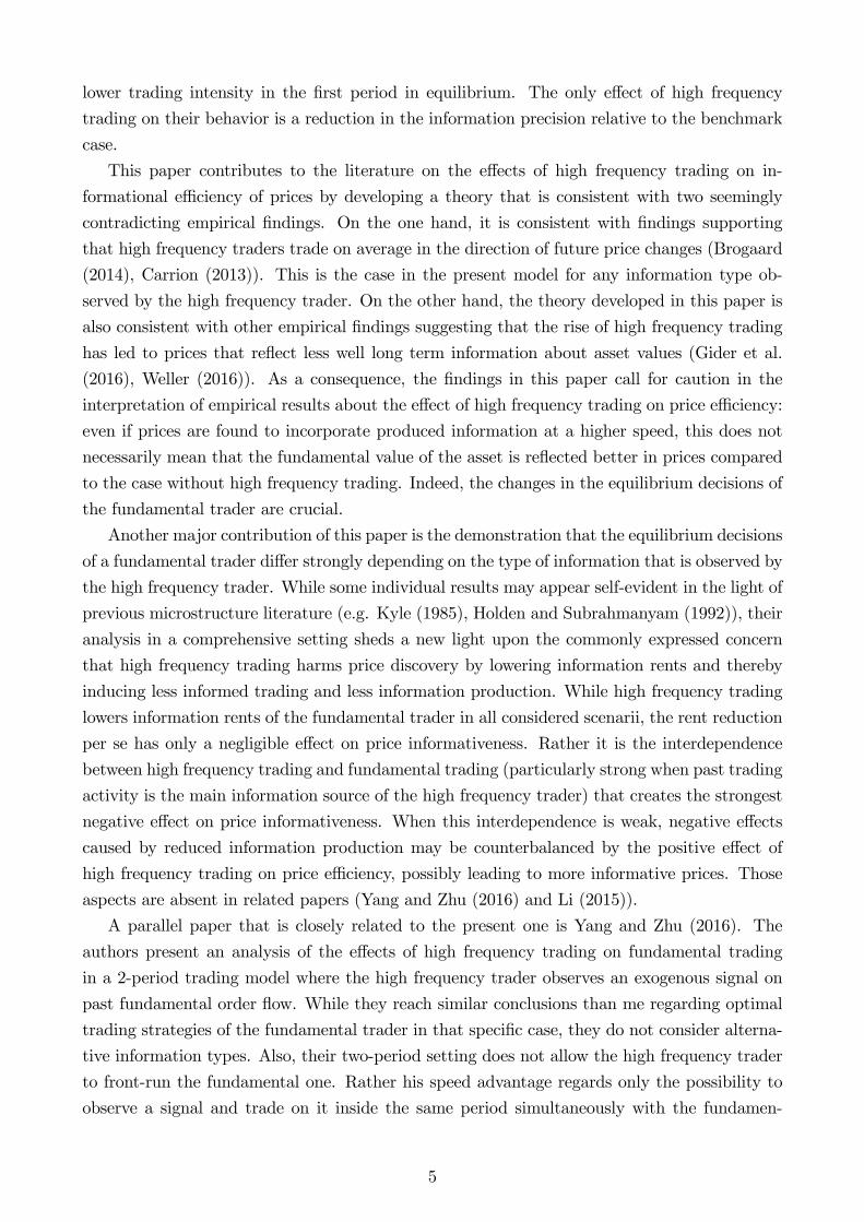
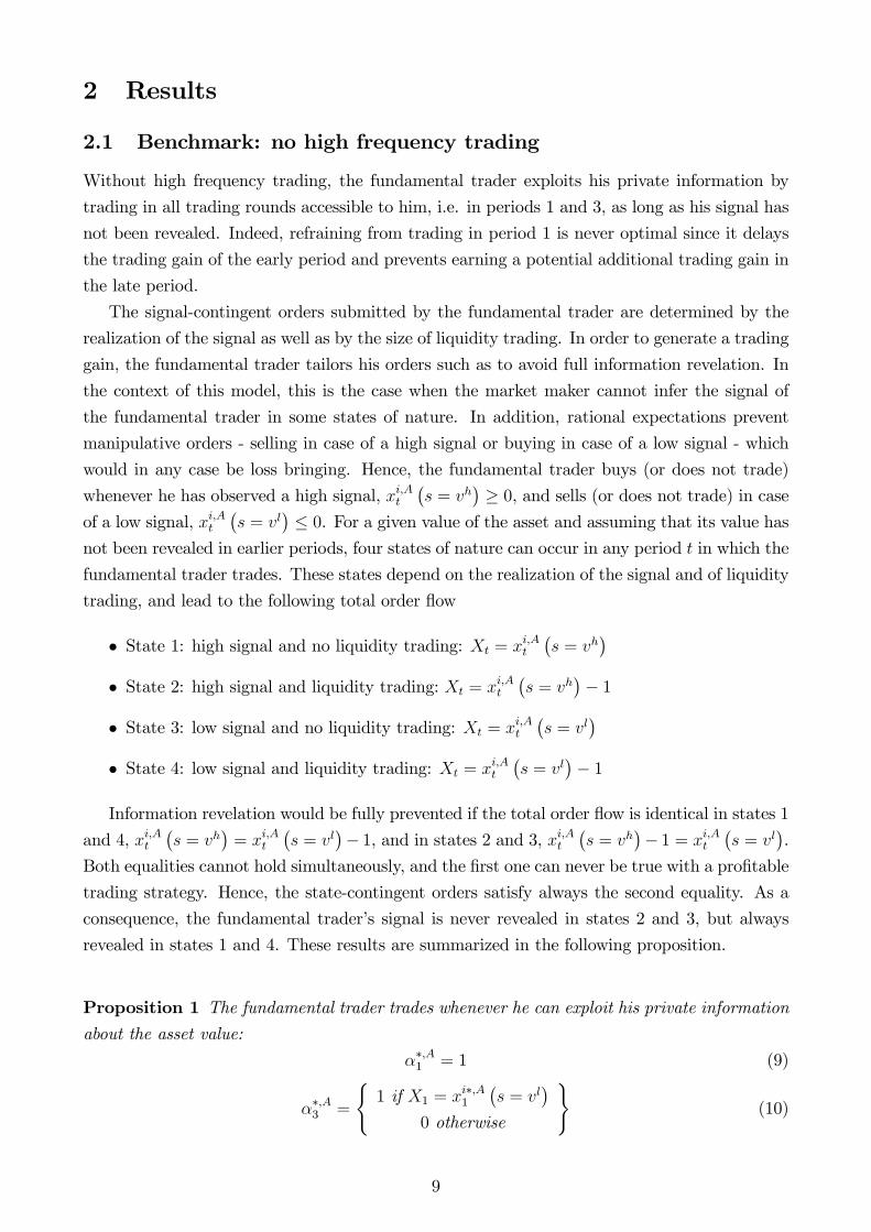
Figure 1 displays the time line of the game.
8
2 Results
2.1 Benchmark: no high frequency trading
Without high frequency trading, the fundamental trader exploits his private information by
trading in all trading rounds accessible to him, i.e. in periods 1 and 3, as long as his signal has
not been revealed. Indeed, refraining from trading in period 1 is never optimal since it delays
the trading gain of the early period and prevents earning a potential additional trading gain in
the late period.
The signal-contingent orders submitted by the fundamental trader are determined by the
realization of the signal as well as by the size of liquidity trading. In order to generate a trading
gain, the fundamental trader tailors his orders such as to avoid full information revelation. In
the context of this model, this is the case when the market maker cannot infer the signal of
the fundamental trader in some states of nature. In addition, rational expectations prevent
manipulative orders - selling in case of a high signal or buying in case of a low signal - which
would in any case be loss bringing. Hence, the fundamental trader buys (or does not trade)
whenever he has observed a high signal, xi,At(s = vh
)≥ 0, and sells (or does not trade) in case
of a low signal, xi,At(s = vl
)≤ 0. For a given value of the asset and assuming that its value has
not been revealed in earlier periods, four states of nature can occur in any period t in which the
fundamental trader trades. These states depend on the realization of the signal and of liquidity
trading, and lead to the following total order flow
• State 1: high signal and no liquidity trading: Xt = xi,At(s = vh
)• State 2: high signal and liquidity trading: Xt = xi,At
(s = vh
)− 1
• State 3: low signal and no liquidity trading: Xt = xi,At(s = vl
)• State 4: low signal and liquidity trading: Xt = xi,At
(s = vl
)− 1
Information revelation would be fully prevented if the total order flow is identical in states 1
and 4, xi,At(s = vh
)= xi,At
(s = vl
)− 1, and in states 2 and 3, xi,At
(s = vh
)− 1 = xi,At
(s = vl
).
Both equalities cannot hold simultaneously, and the first one can never be true with a profitable
trading strategy. Hence, the state-contingent orders satisfy always the second equality. As a
consequence, the fundamental trader’s signal is never revealed in states 2 and 3, but always
revealed in states 1 and 4. These results are summarized in the following proposition.
Proposition 1 The fundamental trader trades whenever he can exploit his private informationabout the asset value:
α∗,A1 = 1 (9)
α∗,A3 =
{1 if X1 = xi∗,A1
(s = vl
)0 otherwise
}(10)
9

The optimal signal-contingent orders have the following properties:
xi∗,At
(s = vh
)≥ 0 and xi∗,At
(s = vl
)≤ 0 with at least one strict inequality (11)
and
xi∗,At
(s = vh
)= 1 + xi∗,At
(s = vl
)(12)
The fundamental trader’s trading gain is identical for any combination of xi∗,At
(s = vh
)and
xi∗,At
(s = vl
)that satisfies the properties formulated in Proposition 1.
With the optimal trading strategy, the total trading gain of the slow trader is increasing
in the signal precision. Hence, the optimally chosen signal precision is limited only by high
information costs.
Proposition 2 The fundamental trader generates a perfectly informative signal if informationcosts are small, and an imperfectly informative signal if they are high. His signal is never
uninformative.
qi∗,A =
{1 if c < cA
12
+3(vh−vl)
8c< 1 if c > cA
}(13)
with cA = 34
(vh − vl
)
2.2 With high frequency trading
In the first trading round, the only informed trader potentially participating in the market
is the fundamental trader. The essence of the results developed in the previous sub-section
carry over to this one, in the sense that it is impossible for the fundamental trader to remain
unrecognized in every state of the world, if he trades. If his signal is correctly inferred by
the market maker in the early period, full information revelation eliminates the scope for high
frequency trading. The following paragraphs describe trading decisions in the case in which
the signal of the fundamental trader is not fully revealed in early trading.
The high frequency trader has an information disadvantage compared to the fundamental
trader with any type of information he observes in any period. The signal of the fundamental
trader is therefore only revealed partially through high frequency trading. Although high
frequency trading lowers the fundamental trader’s expected trading gain in the last period, this
gain never vanishes. Consequently, the fundamental trader exploits his private information in
the last trading round, regardless of whether high frequency trading took place in an earlier
period and regardless of whether the high frequency trader participates in the last trading
round.
The high frequency trader, in turn, always trades in the second period to exploit his private
information, but he cannot design a profitable trading strategy in the last period. Indeed, in
those states of the world in which his signal was inferred by the market maker in the second
10
period, trading in the subsequent period is unprofitable. In those states of the world in which
his signal was not recognized, trading together with the better informed fundamental trader
is always loss bringing. Hence, the high frequency trader exploits his information quickly
before additional fundamental trading takes place, but never trades simultaneously with the
fundamental trader. These results are summarized in the following propositions.
Proposition 3 In period 3, the fundamental trader trades if his signal has not been revealed
in the first period:
α∗,j3 =
{1 if X1 = xi∗,j1
(s = vl
)0 otherwise
}(14)
with j = B,C,D. The signal-contingent orders satisfy the conditions indicated in Proposition
1.
Proposition 4 The high frequency trader never trades in periods 1 and 3. He trades only in
period 2 if the signal of the fundamental trader was not revealed earlier. His signal-contingent
orders satisfy the conditions given in Proposition 1 (replacing s with sf).
These results highlight the importance of considering both differences in information ac-
quisition and differences in trading speeds when the consequences of the coexistence of high
frequency and fundamental (low frequency) trading are analyzed.
While the trading decisions of the fundamental trader do not depend on high frequency
trading in the last trading round, in the first one they are affected by the presence of high
frequency trading and by the type of information the high frequency trader observes. Therefore,
the optimal trading strategies of the fundamental trader in period 1 are analyzed separately
per information type of the high frequency trader.
2.2.1 HFT signal on past trading activity (case B)
When trading took place in the first period (X1 6= 0) and the signal of the fundamental trader
was not fully revealed (X1 6= xi,Bt(s = vl
)− 1; see discussion of the benchmark case), the
high frequency trader obtains a noisy signal on the direction of the order submitted by the
fundamental trader (sell, buy or no trade). Following proposition 1, possible realizations for
sf depend on the strategy chosen by the fundamental trader in the first period and include
the following pairs: {xi1 < 0, xi1 > 0} if the fundamental trader trades with any signal real-ization, {xi1 = 0, xi1 > 0} if the fundamental trader trades only in case of a high signal, and{xi1 < 0, xi1 = 0} if the fundamental trader trades only in case of a low signal. The precision ofthe high frequency trader’s signal, qf , is defined as follows:
Pr(direction
(sf)
= direction(xi1)| direction
(xi1))
= qf (15)
11
As an illustration, consider the following strategies of the fundamental trader: xi1(s = vl
)< 0
and xi1(s = vh
)= 0. If he has observed the low signal and if he decides to trade, he submits
a sell order of one unit in period 1. Hence the total order flow is either X1 = −2, in which
case the low signal is revealed, or X1 = −1, in which case the signal s is not revealed. In the
subsequent period, the high frequency trader becomes active if s was not revealed (X1 = −1).
His signal, sf , indicates then with probability qf that the fundamental trader sold and with
probability 1− qf that liquidity traders sold. If the fundamental trader refrained from trading
in period 1 and X1 = −1 is realized, the high frequency trader attributes the negative total
order flow to the selling activity of liquidity traders with probability qf . This signal determines
the order that the high frequency trader submits in period 2: whenever his signal inidcated that
the fundamental trader sold in the past period, the high frequency trader will sell in period 2.
With the ability of the high frequency trader to detect fundamental trading, the fundamental
trader faces now a new trade-off. If he decides to always trade in the first period, the probability
that the direction of his order is detected in the next period is highest. This leads to price
adjustments in the direction of the true asset value both in period 2 and 3 and thus to a
lower trading gain in period 3. To avoid being detected, the fundamental trader might also
refrain from trading in period 1. If he always refrains from trading, his behavior is rationally
anticipated by the market maker and by the high frequency trader, so that the fundamental
trader’s period 1 trading gain is shifted to period 3. However, the fundamental trader could also
randomize between trading and not trading. In that case, his signal-contingent trading decisions
create additional confusion, since all other traders are less capable to infer his signal from X1.
By doing so, he forgoes some expected trading gains in period 1 but raises his trading gain in
period 3 compared to the case in which he would always trade. In equilibrium, the fundamental
trader always randomizes between trading and not trading in period 1.3 Moreover, the signal-
contingent orders that lead to best hiding mirror exactly liquidity trading: xi∗,B1
(s = vl
)= −1
and xi∗,B1
(s = vh
)= 0. Applying these mixed strategies in period 1 yields several gains to the
fundamental trader. First, the market maker cannot distinguish states where only liquidity
trading takes place from states where the fundamental trader also trades. With any other
combination of orders, the total order flow would systematically differ between those states and
the "hiding" strategy would be less effi cient. As a consequence, the transaction price when the
total order flow is −1 is less effi cient than when the fundamental trader always trades, raising
its profit in case he sells. This, however, cannot be the driving force behind the equilibrium
in mixed strategies since these are never played without high frequency trading although the
same argument would apply. More importantly, mixed strategies modify the behavior of the
high frequency trader. Indeed, he remains inactive more often (whenever the total order flow
3From a technical point of view, the intertemporal expected trading gain earned by the fundamental taderconditional on trading in both periods diminishes in α1 since fundamental trading is on average recognized bythe high frequency trader. However, conditional on not trading in the first period, his expected gain (which isthe period 3 gain) increases in α1 because the fundamental trader trades on average in the opposite direction andpushes prieces away from the fundamental trader’s assessment of the asset value. At the equilibrium value α∗,B1 ,the fundamental trader is indifferent between trading and not trading in the first period (i.e. both expectedtrading gains are equal).
12

is zero, which can happen here with any signal realization s). In addition, he trades on average
in the wrong direction in the state where the fundamental trader observes a low signal but
refrains from trading, and the total order flow is −1 and correctly recognized as coming from
liquidity trading. By inducing the high frequency trader in error, the fundamental trader raises
his information rent in period 3. These results are summarized in the following proposition.
Proposition 5 In period 1, the fundamental trader optimally randomizes between trading and
not trading:1
2< α∗,B1 < 1 (16)
The expression for α∗,B1 is indicated in the appendix. When he trades, the signal-contingent
orders are as follows:
xi∗,B1
(s = vh
)= 0 (17)
xi∗,B1
(s = vl
)= −1
Consistent with the fact that the mixed strategies are primarily driven by to possibility to
blur the high frequency trader, the likelihood to trade in period 1, α∗,B1 , depends only on the
precision of the high frequency trader’s signal, qf .
Lemma 1 The probability to trade in period 1 is only determined by the likelihood to be detected
by the fast trader in the subsequent period: α∗,B1 depends only on qf , with ∂α∗,B1∂qf
< 0.
In every trading round, the gain obtained by the fundamental trader, if he trades, increases in
his signal precision. However, the existence of the high frequency trader and the implementation
of mixed strategies lower his overall gains. This results in a signal precision that starts declining
at lower costs than in the benchmark case (cB < cA) and is hence smaller up from the cost
threshold cB.
Proposition 6 The fundamental trader generates a perfectly informative signal if informationcosts are small, and an imperfectly informative signal if they are high. His signal is never
uninformative:
qi∗,B =
{1 if c < cB
= 12
+(vh−vl)16c
Φ(qf)if c > cB
}(18)
with cB and Φ(qf)given in the appendix.
13
2.2.2 HFT signal on fundamental trader’s information (case C)
We now consider an alternative case in which the high frequency trader can observe noisy
information about the signal observed by the fundamental trader (instead of the direction of
his order flow as in the previous sub-section). The precision of the high frequency trader’s
signal is then defined as follows:
Pr(sf : s = vh | s = vh
)= Pr
(sf : s = vl | s = vl
)= qf (19)
Differently to the previous case, this information is not about a realized transaction. Hence, it
does not depend on the trading decision of the fundamental trader in the first period. Even if
he plays mixed strategies, he cannot induce the high frequency trader to trade in the opposite
direction to the one implied by his signal. Indeed, in the state in which the fundamental trader
observes a low signal but decides not to trade, the high frequency trader trades in the “right”
direction on average when the total order flow is −1, in contrast to the previous case in which
he would trade in the “wrong”direction. The only benefit of mixed strategies here, is a lower
scrutiny by the high frequency trader. This effect, however, is not large enough to effectively
lead to the implementation of mixed strategies in equilibrium. In conclusion, the seemingly
small twist in the information structure of the high frequency trader induces a substantial
change in the behavior of the fundamental trader who always trades upon his information in
the first period in equilibrium.4
Proposition 7 The fundamental trader never refrains from trading in period 1: α∗,C1 = 1. The
optimal signal contingent orders are determined by the conditions given in proposition 1.
The difference in optimal trading strategies between case B and case C imply a different
split of the fundamental trader’s expected trading gains over time. In case B, the share of
the total expected trading gain realized in period 1 is larger than the share realized in period
3, as long as the high frequency trader observes a rather uninformative signal (qf close to12). However, the first period’s share declines as qf increases and becomes smaller than the
period 3 share when qf is close to 1. Indeed, the more accurately the high frequency trader can
recognize fundamental order flow, the more the fundamental trader pushes the realization of
trading gains to the last period. In case C, the opposite takes place. Not only is the share of
the expected trading gain realized in period 1 always larger than the one realized in period 3,
it also increases with qf . The more accurately the high frequency trader can observe the signal
of the fundamental trader, the smaller is the period 3 trading gain and consequently its share
in the total expected trading gain.
When the high frequency trader has information about the fundamental trader’s signal,
the latter cannot "hide" effi ciently by playing mixed strategies. Consequently, he collects
4Notice that the implications of a signal on fundamental order flow and a signal on fundamental informationare equivalent if the fundamental trader always trades upon his signal - i.e. when α = 1.
14
information with a high enough precision to generate a large trading gain in the first trading
round. The optimal signal precision is lower than in the benchmark case (due to high frequency
trading that always lowers the expected trading gain in the third period) but higher then in
case B.
Proposition 8 The fundamental trader generates a perfectly informative signal if informationcosts are small, and an imperfectly informative signal if they are high. His signal is never
uninformative:
qi∗,C =
{1 if c < cC
12
+(vh−vl)(5+4(1−qf)qf
16cif c > cC
}(20)
with cC =(5+4(1−qf)qf(vh−vl)
8.
2.2.3 Comparison across cases A, B and C
Changes in the behavior of the fundamental trader depend crucially on the type of information
observed by the high frequency trader. Comparing his decision on the signal precision, it
is always the highest in the benchmark case, followed by case C and eventually by case B
(qi∗,A ≥ qi∗,C ≥ qi∗,B). Also, the cost threshold up from which the optimal precision diminishes
with increasing costs is highest in the benchmark case and lowest in case B (cB < cC < cA).
Corollary 1 With high frequency trading, the fundamental trader collects equally or less preciseinformation than without high frequency trading:
qi∗,j = qi∗,A = 1 if c < cj (21)
qi∗,j < qi∗,A = 1 if cj < c < cA
qi∗,j < qi∗,A < 1 if c > cA
with j = B,C .
Turning to the trading strategy in the early trading round, it is only altered in case B
relative to the benchmark, since the fundamental trader optimally plays mixed strategies.
Corollary 2 Comparison of trading probabilities in t = 1:
α∗,A1 = α∗,C1 = 1 (22)
α∗,B1 < 1 (23)
15
Considering the comparisons in Corollaries 1 and 2, high frequency trading has no impact
on fundamental trading when the information of the high frequency trader is about the signal
observed by the fundamental trader (case C) and when information costs are suffi ciently small.
Indeed, in this case the fundamental trader collects always perfectly precise information and
trades always on this information in the first trading round. Changes in fundamental trading
occur either in case C when information costs are high (the fundamental reduces the precision of
his signal more than in the benchmark case), or when the high frequency trader can detect the
direction of past fundamental trading (case B), in which case the fundamental trader reduces
both his signal precision (with high costs) and his trading intensity.
2.2.4 Effects on the informativeness and effi ciency of prices
The analysis of optimal trading strategies and of fundamental information production suggests
that the effects of high frequency trading on how well the prices reflect the asset value vary
depending on the information type observed by the high frequency trader and depending on
the information costs borne by the fundamental trader. To assess these effects, I compute
two measures. The first one measures how well prices reflect the fundamental value of the
asset (price informativeness or PI ). It is calculated by computing the average pricing errors
(in absolute terms) per period, benchmarking these to the highest pricing errors possible in
this model (i.e. those that realize in the absence of any informed trading) and substracting the
resulting number from 1:
PIt ≡ 1− E0[|v − pt||v − µ|
](24)
The expectation is taken over all asset values and signal realizations. If this measure is equal to
1, the average pricing error relative to the true value of the asset is zero, hence prices are fully
informative about the asset value. If this measure is equal to zero, prices are uninformative
since average pricing errors are the same as without any informed trading.
The second measure captures how much of the information produced by the fundamental
trader is incorporated in prices (price effi ciency or PE). To compute it, a similar method as
for price informativeness is employed. However, pricing errors are computed relative to the
expected asset value conditional on the observed signal s. Indeed, if the fundamental trader
observes for instance the signal s = vh, the expected asset value, vhqi + vl(1− qi), correspondsto the produced fundamental information. A portion of this value is reflected in prices. This is
measured as follows:
PEt ≡ 1− E0[|E [v | s]− pt||E [v | s]− µ|
](25)
If this measure is equal to 1, prices reflect fully the signal observed by the fundamental trader.
If it is equal to zero, the signal is not incorporated in prices.
As expected, both price informativeness and price effi ciency increase in every period in
which informed trading takes place. In case of the benchmark:
PIA1 = PIA2 < PIA3 and PEA1 = PEA
2 < PEA3 (26)
16
and with the existence of high frequency trading:
PIj1 < PIj2 < PIj3 and PEj1 < PEj
2 < PEj3 for j = B,C (27)
A comparison across cases yields the following results.
Proposition 9 When the high frequency trader observes a signal about the fundamental orderflow (case B), both price informativeness and price effi ciency are worse than without high
frequency trading (case A) in every period:
PIBt < PIAt , ∀t (28)
PEBt < PEA
t , ∀t (29)
Case B illustrates the combination of two negative effects created by the existence of high
frequency trading: the fundamental trader hides his trades more than in the benchmark case,
which lowers the portion of the produced fundamental information that is incorporated in the
price. As a consequence, his trading profits diminish leading to less information generation
when costs are suffi ciently high. The additional hiding leads to lower price effi ciency and this
combined with possibly less information production leads to lower price informativeness. Since
these results hold for any precision level (i.e. also when information costs are small enough
to allow a perfectly precise signal), their main driver is the reduced intensity of fundamental
trading in the first period.
Interestingly, price effi ciency and informativeness are also reduced relative to the benchmark
in the second period. In this period, no additional information would have been incorporated
in the price in the benchmark case, while some additional information is always incorporated
with high frequency trading. Hence, price effi ciency and informativeness never improve in the
benchmark case, while they do in case B. However, despite this improvement, the mixed strate-
gies played by the fundamental trader in the first period lead to such an ineffi cient (and hence
uninformative) price in that period, that the added information through high frequency trading
in the subsequent period does not make the price more effi cient and informative compared to
the benchmark.
This finding reconciles empirical evidence suggesting that high frequency traders tend to
trade in the direction of permanent price changes (Brogaard et al. (2014)) with other evidence
indicating that long term information is less well reflected by prices after the rise of high
frequency trading (Weller (2016), Gider et al. (2016)). Here, the high frequency trader trades
on average in the right direction and contributes to improve price informativeness over time
inside case B. However, compared to the benchmark, less information is eventually reflected
by the price and information is incorporated at a slower pace, supporting the second piece
of evidence mentioned earlier. Hence, this finding calls for caution in the interpretation of
empirical results about the effect of high frequency trading on price effi ciency: even if it is
17
found to incorporate information in prices at a higher frequency (thus raising price effi ciency
at a high speed), this does not necessarily mean that the fundamental value of the asset is
reflected better in prices as compared to the case without high frequency trading. Indeed, the
equilibrium response of fundamental traders is crucial.
Turning to the case in which the high frequency trader observes information about the signal
of the fundamental trader (case C), the effect on price effi ciency is the opposite of case B: it
increases in every period relative to the benchmark. This illustrates the positive influence of high
frequency trading that leads to the incorporation of more produced fundamental information
in prices over time.
Proposition 10 When the high frequency trader observes a signal about the information ofthe fundamental trader (case C), price effi ciency is identical to the benchmark case in the first
period, but increases always in the subsequent periods.
PEC1 = PEA
1 (30)
PEC2 > PEA
2 (31)
PEC3 > PEA
3 (32)
The effects of high frequency trading on the informativeness of prices are more nuanced.
Although in this case, the trading strategy of the fundamental trader never changes compared to
the benchmark (he does not hide his trades more than in the benchmark case), he produces less
information if information costs are high. Hence, the improvement in price effi ciency thanks to
high frequency trading might be counter-balanced by less information production, resulting in
ultimately less informative price. This reduction in price informativeness happens specifically
in those periods in which the fundamental trader is active on the market, since he trades
upon a less informative signal. In the second period, in which only the high frequency trader
trades, price informativeness is always increased. Summarizing, prices are more informative on
average compared to the benchmark, when the information cost is small enough. Otherwise,
price informativeness is reduced on average.
Proposition 11 When the high frequency trader observes a signal about the information of thefundamental trader (case C), price informativeness never improves in the first trading period
but improves always in the second period. The effect in the third period depends on c.
PIC1 = PIA1 if c ≤ cC (33)
PIC1 < PIA1 if c > cC
PIC2 > PIA2 (34)
18
PIC3 > PIA3 if c ≤ cT (35)
PIC3 < PIA3 if c > cT (36)
with cC < cT < cA.
This case contrasts with case B regarding the dynamics of price effi ciency and informative-
ness. While in case B price effi ciency is lower than in the benchmark case at all dates, i.e.
a smaller portion of the fundamental signal is incorporated in prices at all dates, it is always
(weakly) higher in case C. However, when price informativeness is considered, this case features
a disconnect between the speed at which prices reflect (partially) the actual asset value and the
portion of that value that is ultimately incorporated in the price. Since price informativeness is
always higher in the second period, the price reflects a higher portion of the actual fundamental
value of the asset than in the benchmark case. However, when price informativeness is lower
in the third period, eventually the price reflects less well the asset value. Hence, with small
information costs, the price reflects better the asset value and this incorporation of information
occurs at a higher speed than in the benchmark. With high information costs, some information
is incorporated at a higher speed, but the price reflects less well the asset value eventually.
These results shed a new light upon the commonly expressed concern that high frequency
trading harms price discovery by lowering information rents and thereby inducing less informed
trading and less information production. While high frequency trading lowers information
rents of the fundamental trader in all considered scenarii, the rent reduction per se has only
a negligible effect on price informativeness. Rather it is the interdependence between high
frequency trading and fundamental trading (particularly strong when past trading activity is
the main information source of the high frequency trader - case B) that creates the strongest
negative effect on price informativeness. When this interdependence is weak (case C), negative
effects caused by reduced information production may be counterbalanced by the positive effect
of high frequency trading on price effi ciency, possibly leading to more informative prices.
2.2.5 Learning from a second exchange (case D)
In the analysis so far, the high frequency trader observed information signals with a precision
that is independent of the trading choices of other traders. This assumption is justifiable if
the information is gathered by screening e.g. news posts. However, it is debatable if high
frequency traders obtain their information by screening order flow and transactions on other
markets as these are the outcomes of endogenous trading decisions. It seems plausible that
market data becomes less informative about fundamental trading the higher the propensity of
fundamental traders is to refrain from trading by playing mixed strategies and hide thereby
their information.
To address this issue, the basiline model is extended to allow the high frequency trader to
observe previous transactions on two exchanges: the main exchange analyzed on which he is
19
active denoted by exchange y and an additional exchange that has the same characteristics as
the main one denoted by exchange z. Trading is organized identically on each exchange such that
exchange z is a duplicate of the exchange described in the baseline model. In particular, there
is no multi-market trading. Rather, the additional exchange is only an additional information
source for the high frequency trader on exchange y. To simplify the analysis, I assume that the
fundamental trader on exchange z observes the same signal realization as the one on exchange
y. Also, both choose the same trading strategies: the size of signal-contingent orders and the
randomization probability α. Without loss of generality, I consider trading strategies of the
fundamental traders that foresee no trading in case of the high signal and selling −1 in case of
the low signal if they decide to trade. However, the realized total order flow can differ between
both exchanges for two reasons. First, the realization of liquidity trading is independent on
each exchange. Second, if fundamental traders choose to randomize between trading and not
trading (α < 1), their actions are independent from each other: fundamental trading might
then take place on one exchange but not on the other. Moreover, to guarantee that the high
frequency trader has more information about informed trading than the market maker on the
main exchange, the latter is assumed to be unable to observe past transactions on the other
exchange.
In this environment, the information of the high frequency trader on exchange y consists
in the realized past transactions on both exchanges. To keep consistency with the previous
analysis, the high frequency trader starts searching for additional information only if trading
took place on exchange y in period 1 (Xy1 6= 0) and was not fully informative (Xy
1 = −1). The
high frequency trader assesses the likelihood that trading on exchange y originated from the
fundamental trader conditional on observing the order flow on exchange z:
Pr (Xy1 = −1 is fundamental trading | Xz
1 ) (37)
where the total order flow on the second exchange can take three different values: Xz1 =
{−2,−1, 0}.Taking the perspective of the fundamental trader (on exchange y), he determines his signal
precision and his trading strategy in the early trading round before Xz1 is realized. Hence,
he forms an expectation of the likelihood with which his order will be detected by the high
frequency trader in the intermediate period. The average posterior belief of the high frequency
trader on fundamental trading on exchange y is not necessarily identical in each state of the
world whereXy1 = −1 occurs. Indeed, depending on whether the high signal was observed (state
a), the low signal was observed and the fundamental trader on exchange y traded (state b), or
the low signal was observed and the fundamental trader on exchange y refrained from trading
(state c), the high frequency trader observes different order flow combinations on exchange y and
z with different probabilities. It turns out that the average posterior belief that fundamental
trading took place in the first period on exchange y is perfectly correlated with the signal
20
observed by the fundamental traders:
E [Pr (Xy1 = −1 is fundamental trading | Xz
1 ) | state a] =1
2+
3
4α− 1
2− α (38)
E [Pr (Xy1 = −1 is fundamental trading | Xz
1 ) | state k] =α(4− α)
4(2− α)with k = b, c (39)
The previous analysis suggests that this discourages the fundamental traders from hiding their
trades by playing mixed strategies. However, the likelihood to be recognized increases with the
probability to trade, α, when the low signal was observed. Hence, the more likely it is that
fundamental trading takes place whenever the low signal was observed, the more frequently
the high frequency trader detects fundamental trading in the subsequent period. This dynamic
should induce fundamental traders to lower their probability of trading α. However, funda-
mental traders never play mixed strategies in the first period in equilibrium. Although their
trading gain decreases in α if they trade in both periods, but increases in α if they trade only
in the last period, there is no value for α < 1 that makes them indifferent between trading and
not trading in the first period.
Proposition 12 The fundamental trader never plays mixed strategies in the first period:
α∗,D1 = 1 (40)
Similar to the previous cases, information precision always raises the fundamental trader’s
expected profit. Hence, he lowers the precision only if information costs are suffi ciently high.
Proposition 13 The fundamental trader generates a perfectly informative signal if informationcosts are small, and an imperfectly informative signal if they are high. His signal is never
uninformative:
qi∗,D =
{1 if c < cD
= 12
+23(vh−vl)
64cif c > cD
}(41)
with cD =23(vh−vl)
32.
Compared to the benchmark case, the optimal signal precision starts declining up from a
lower cost level and remains at a lower level.
Corollary 3 The precision is equal or lower than in the benchmark case:
qi∗,D = qi∗,A = 1 if c < cD (42)
qi∗,D < qi∗,A = 1 if cD < c < cA
qi∗,D < qi∗,A ≤ 1 if c > cA
21
3 Conclusion
I develop a multi-period trading model to analyze how a fundamental trader adjusts his trad-
ing strategies and information production decisions to the existence of high frequency trading
(HFT). I show that these decisions differ strongly depending on the type of information that
the HFT can observe. Information correlated with past trading activity reduces fundamental
trading and information production, and leads to lower price informativeness, compared to a
benchmark without HFT. HFT information correlated with fundamental information does not
induce these effects, and prices may become more informative on average. Moreover, I study
the ability of prices to reflect the asset value and produced information over time. My results
are consistent with empirical findings highlighting that HFT enhances price discovery in the
short run, and others suggesting that HFT reduces the ability of prices to reflect long-term
fundamental information.
22
References
Baldauf, M. and Mollner, J., 2015. High-frequency trading and market performance.
Biais, B., Foucault, T. and Moinas, S., 2015. Equilibrium fast trading. Journal of Financial
Economics, 116(2), pp.292-313.
Biais, B. andWoolley, P., 2011. High frequency trading. Manuscript, Toulouse University, IDEI.
Brogaard, J., Hendershott, T. and Riordan, R., 2014. High-frequency trading and price discov-
ery. Review of Financial Studies, 27(8), pp.2267-2306.
Budish, E., Cramton, P. and Shim, J., 2015. The high-frequency trading arms race: Frequent
batch auctions as a market design response. The Quarterly Journal of Economics, 130(4),
pp.1547-1621.
Carrion, A., 2013. Very fast money: High-frequency trading on the NASDAQ. Journal of
Financial Markets, 16(4), pp.680-711.
Clark-Joseph, A., 2014. Exploratory trading. Harvard University, Cambridge MA.
Foucault, T., Hombert, J. and Rosu, I., 2016. News trading and speed. The Journal of Finance,
71(1), pp.335-382.
Gider, J., Schmickler, S.N. and Westheide, C., High-Frequency Trading and Fundamental Price
Effi ciency.
Gomber, P., Arndt, B., Lutat, M. and Uhle, T., 2011. High-frequency trading.
Hirschey, N., 2016. Do high-frequency traders anticipate buying and selling pressure?.
Hagströmer, B. and Norden, L., 2013. The diversity of high-frequency traders. Journal of Fi-
nancial Markets, 16(4), pp.741-770.
Holden, C.W. and Subrahmanyam, A., 1992. Long-lived private information and imperfect
competition. The Journal of Finance, 47(1), pp.247-270.
Kyle, A.S., 1985. Continuous auctions and insider trading. Econometrica: Journal of the Econo-
metric Society, pp.1315-1335.
Menkveld, A. J., 2016. The Economics of High-Frequency Trading: Taking Stock. Annual
Review of Financial Economics, Volume 8, Forthcoming.
Weller, B.M., 2016. Effi cient prices at any cost: does algorithmic trading deter information
acquisition?.
Yang, L. and Zhu, H., 2016. Back-running: Seeking and hiding fundamental information in
order flows.
23
Appendix
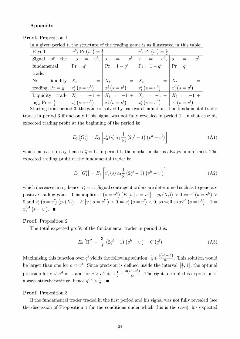
Proof. Proposition 1In a given period t, the structure of the trading game is as illustrated in this table:Payoff vh, Pr
(vh)
= 12
vl, Pr(vl)
= 12
Signal of the
fundamental
trader
s = vh,
Pr = qis = vl,
Pr = 1− qis = vh,
Pr = 1− qis = vl,
Pr = qi
No liquidity
trading, Pr = 12
Xt =
xit(s = vh
) Xt =
xit(s = vl
) Xt =
xit(s = vh
) Xt =
xit(s = vl
)Liquidity trad-
ing, Pr = 12
Xt = −1 +
xit(s = vh
) Xt = −1 +
xit(s = vl
) Xt = −1 +
xit(s = vh
) Xt = −1 +
xit(s = vl
)Starting from period 3, the game is solved by backward induction. The fundamental trader
trades in period 3 if and only if his signal was not fully revealed in period 1. In that case his
expected trading profit at the beginning of the period is:
E3[Gi3
]= E3
[xi3 (s)α3
1
16
(2qi − 1
) (vh − vl
)](A1)
which increases in α3, hence α∗3 = 1. In period 1, the market maker is always uninformed. The
expected trading profit of the fundamental trader is:
E1[Gi1
]= E1
[xi1 (s)α1
1
8
(2qi − 1
) (vh − vl
)](A2)
which increases in α1, hence α∗1 = 1. Signal contingent orders are determined such as to generate
positive trading gains. This implies xit(s = vh
) (E[v | s = vh
]− pt (Xt)
)> 0 ⇔ xit
(s = vh
)>
0 and xit(s = vl
) (pt (Xt)− E
[v | s = vl
])> 0⇔ xit
(s = vl
)< 0, as well as xi,At
(s = vh
)−1 =
xi,At(s = vl
).
Proof. Proposition 2The total expected profit of the fundamental trader in period 0 is:
E0[Πi]
=3
16
(2qi − 1
) (vh − vl
)− C
(qi)
(A3)
Maximizing this function over qi yields the following solution: 12
+3(vh−vl)
8c. This solution would
be larger than one for c < cA. Since precision is defined inside the interval[12, 1], the optimal
precision for c < cA is 1, and for c > cA it is 12
+3(vh−vl)
8c. The right term of this expression is
always strictly positive, hence qi,∗ > 12.
Proof. Proposition 3If the fundamental trader traded in the first period and his signal was not fully revealed (see
the discussion of Proposition 1 for the conditions under which this is the case), his expected
24
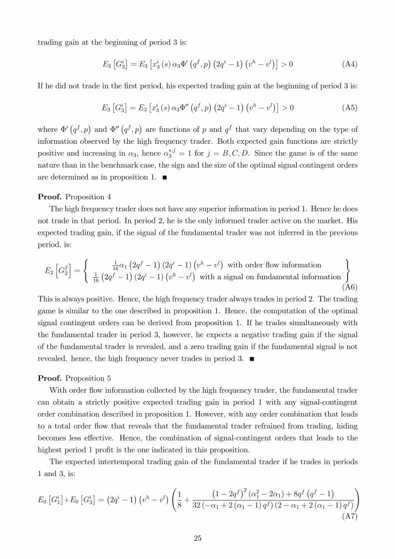
trading gain at the beginning of period 3 is:
E3[Gi3
]= E3
[xi3 (s)α3Φ
′ (qf , p) (2qi − 1) (vh − vl
)]> 0 (A4)
If he did not trade in the first period, his expected trading gain at the beginning of period 3 is:
E3[Gi3
]= E3
[xi3 (s)α3Φ
′′ (qf , p) (2qi − 1) (vh − vl
)]> 0 (A5)
where Φ′(qf , p
)and Φ′′
(qf , p
)are functions of p and qf that vary depending on the type of
information observed by the high frequency trader. Both expected gain functions are strictly
positive and increasing in α3, hence α∗,j3 = 1 for j = B,C,D. Since the game is of the same
nature than in the benchmark case, the sign and the size of the optimal signal contingent orders
are determined as in proposition 1.
Proof. Proposition 4The high frequency trader does not have any superior information in period 1. Hence he does
not trade in that period. In period 2, he is the only informed trader active on the market. His
expected trading gain, if the signal of the fundamental trader was not inferred in the previous
period, is:
E2
[Gf2
]=
{116α1(2qf − 1
)(2qi − 1)
(vh − vl
)with order flow information
116
(2qf − 1
)(2qi − 1)
(vh − vl
)with a signal on fundamental information
}(A6)
This is always positive. Hence, the high frequency trader always trades in period 2. The trading
game is similar to the one described in proposition 1. Hence, the computation of the optimal
signal contingent orders can be derived from proposition 1. If he trades simultaneously with
the fundamental trader in period 3, however, he expects a negative trading gain if the signal
of the fundamental trader is revealed, and a zero trading gain if the fundamental signal is not
revealed. hence, the high frequency never trades in period 3.
Proof. Proposition 5With order flow information collected by the high frequency trader, the fundamental trader
can obtain a strictly positive expected trading gain in period 1 with any signal-contingent
order combination described in proposition 1. However, with any order combination that leads
to a total order flow that reveals that the fundamental trader refrained from trading, hiding
becomes less effective. Hence, the combination of signal-contingent orders that leads to the
highest period 1 profit is the one indicated in this proposition.
The expected intertemporal trading gain of the fundamental trader if he trades in periods
1 and 3, is:
E0[Gi1
]+E0
[Gi3
]=(2qi − 1
) (vh − vl
)(1
8+
(1− 2qf
)2(α21 − 2α1) + 8qf
(qf − 1
)32 (−α1 + 2 (α1 − 1) qf ) (2− α1 + 2 (α1 − 1) qf )
)(A7)
25
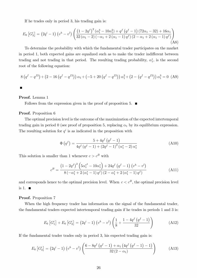
If he trades only in period 3, his trading gain is:
E0[Gi3
]=(2qi − 1
) (vh − vl
)( (1− 2qf)2
(α31 − 10α21) + qf(qf − 1
)(72α1 − 32) + 16α1
32 (α1 − 2) (−α1 + 2 (α1 − 1) qf ) (2− α1 + 2 (α1 − 1) qf )
)(A8)
To determine the probability with which the fundamental trader participates on the market
in period 1, both expected gains are equalized such as to make the trader indifferent between
trading and not trading in that period. The resulting trading probability, α∗1, is the second
root of the following equation:
8(qf − qf2
)+(2− 16
(qf − qf2
))α1+
(−5 + 20
(qf − qf2
))α21+
(2−
(qf − qf2
))α31 = 0 (A9)
Proof. Lemma 1Follows from the expression given in the proof of proposition 5.
Proof. Proposition 6The optimal precision level is the outcome of the maximization of the expected intertemporal
trading gain in period 0 (see proof of proposition 5, replacing α1 by its equilibrium expression.
The resulting solution for qi is as indicated in the proposition with
Φ(qf)
=5 + 4qf
(qf − 1
)4qf (qf − 1) + (2qf − 1)2 (α∗1 − 2)α∗1
(A10)
This solution is smaller than 1 whenever c > cB with
cB =
(1− 2qf
)2 (5α∗
2
1 − 10α∗1
)+ 24qf
(qf − 1
) (vh − vl
)8 (−α∗1 + 2 (α∗1 − 1) qf ) (2− α∗1 + 2 (α∗1 − 1) qf )
(A11)
and corresponds hence to the optimal precision level. When c < cB, the optimal precision level
is 1.
Proof. Proposition 7When the high frequency trader has information on the signal of the fundamental trader,
the fundamental traders expected intertemporal trading gain if he trades in periods 1 and 3 is:
E0[Gi1
]+ E0
[Gi3
]=(2qi − 1
) (vh − vl
)(1
8+
1− 4qf(qf − 1
)32
)(A12)
If the fundamental trader trades only in period 3, his expected trading gain is:
E0[Gi3
]=(2qi − 1
) (vh − vl
)(6− 8qf(qf − 1
)+ α1
(4qf(qf − 1
)− 1)
32 (2− α1)
)(A13)
26
For any α1 ∈ [0, 1], E0 [Gi1] + E0 [Gi
3] > E0 [Gi3]. Hence the optimal trading probability in this
case is α∗,C1 = 1.
Proof. Proposition 8The optimal signal precision results from the maximization of the fundamental traders
expected intertemporal profit in period 0:
E0[Πi]
= E0[Gi1
]+ E0
[Gi3
]− C
(qi)
(A14)
When c < cC the solution to this maximization problem is larger than one, hence qi∗,C = 1.
Otherwise qi∗,C = 12
+(vh−vl)(5+4(1−qf)qf
16c.
27
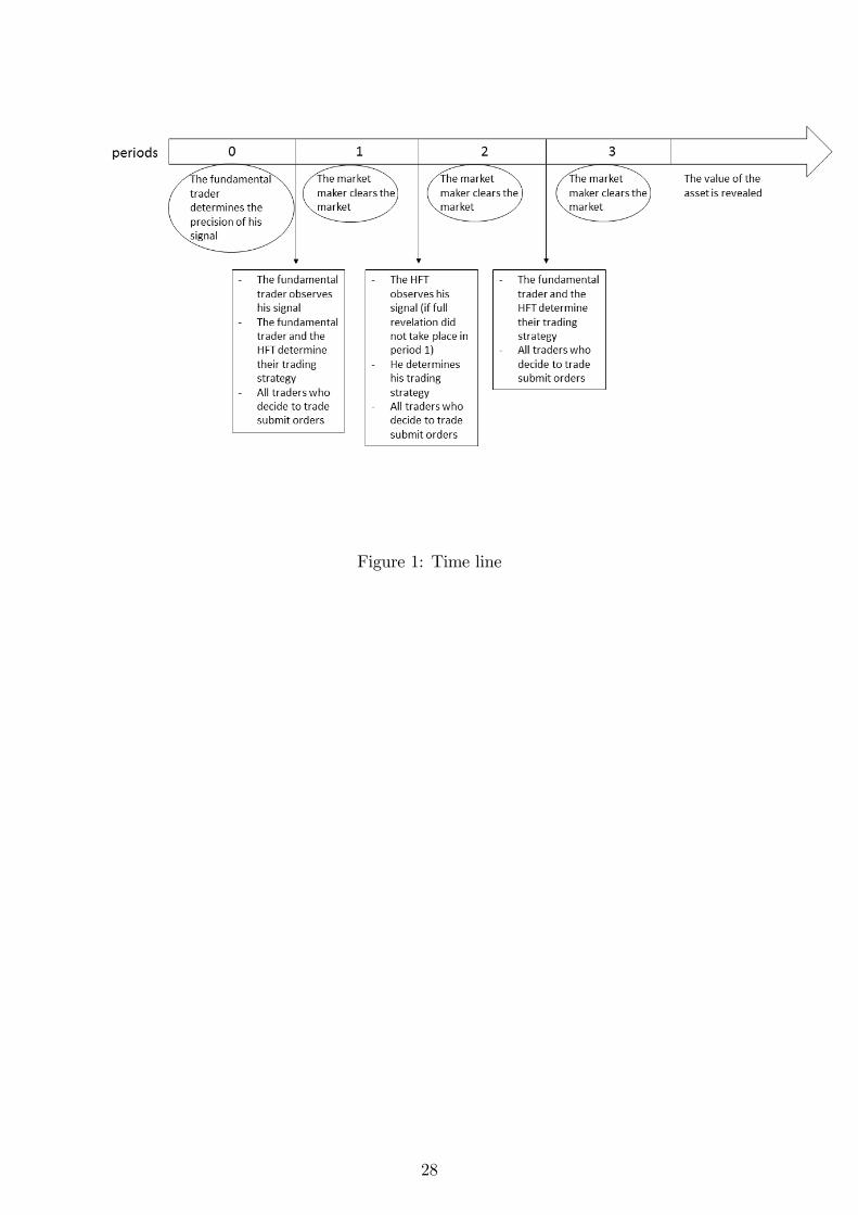
Figure 1: Time line
28