High-fidelity Hydrodynamic Shape Optimization of a 3-D Hydrofoil

Nitin Garga, Gaetan K. W. Kenwayb, Zhoujie Lyub, Joaquim R. R. A. Martinsb, Yin L. Younga,1

aDepartment of Naval Architecture and Marine Engineering, University of Michigan, MI 48109, USAbDepartment of Aerospace Engineering, University of Michigan, MI 48109, USA

Abstract

With recent advances in high performance computing, computational fluid dynamics (CFD) modeling has becomean integral part in the engineering analysis and even in the design process of marine vessels and propulsors. Inaircraft wing design, CFD has been integrated with numerical optimization and adjoint methods to enable high-fidelityaerodynamic shape optimization with respect to large numbers of design variables. There is a potential to use someof these techniques for maritime applications, but there are new challenges that need to be addressed to realize thatpotential. This work presents a solution to some of those challenges by developing a CFD-based hydrodynamic shapeoptimization tool that considers cavitation and a wide range of operating conditions. A previously developed 3-Dcompressible Reynolds-averaged Navier–Stokes (RANS) solver is extended to solve for nearly incompressible flows,using a low-speed preconditioner. An efficient gradient-based optimizer and the adjoint method are used to carry outthe optimization. The modified CFD solver is validated and verified for a tapered NACA 0009 hydrofoil. The needfor a large number of design variables is demonstrated by comparing the optimized solution obtained using differentnumber of shape design variables. The results showed that at least 200 design variables are needed to get a convergedoptimal solution for the hydrofoil considered. The need for a high-fidelity hydrodynamic optimization tool is alsodemonstrated by comparing RANS-based optimization with Euler-based optimization. The results show that at highlift coefficient (CL) values, the Euler-based optimization leads to a geometry that cannot meet the required lift at thesame angle of attack as the original foil due to inability of the Euler solver to predict viscous effects. Single-pointoptimization studies are conducted for various target CL values, and compared with the geometry and performanceof the original NACA 0009 hydrofoil, as well as with the results from a multipoint optimization study. A total of210 design variables are used in the optimization studies. The optimized foil is found to have a much lower negativesuction peak, and hence delayed cavitation inception, in addition to higher efficiency, compared to the original foil atthe design CL value. The results show significantly different optimal geometry for each CL, which means an activemorphing capability was needed to achieve the best possible performance for all conditions. For the single-pointoptimization, using the highest CL as the design point, the optimized foil yielded the best performance at the designpoint, but the performance degraded at the off-design CL points compared to the multipoint design. In particular,the foil optimized for the highest CL showed inferior performance even compared to the original foil at the lowestCL condition. On the other hand, the multipoint optimized hydrofoil was found to perform better than the originalNACA 0009 hydrofoil over the entire operation profile, where the overall efficiency weighted by the probability ofoperation at each CL, is improved by 14.4%. For the multipoint optimized foil, the geometry remains fixed throughout the operation profile and the overall efficiency was only 1.5% lower than the hypothetical actively morphed foilwith the optimal geometry at each CL. The new methodology presented herein has the potential to improve the designof hydrodynamic lifting surfaces such as propulsors, hydrofoils, as well as hulls.

Keywords: shape optimization, high-fidelity, gradient-based optimization, cavitation, single-point optimization,multipoint optimization, hydrofoil, propulsor.

Nomenclature

α Angle of attack, [o]

@ Cell volume, [m3]

νf Fluid kinematic viscosity, [m2{s]

1Corresponding author, email address for correspondence: ylyoung@umich.edu

Preprint submitted to Journal of Ship Research December 11, 2015

ρf Fluid density, [kg{m3]

σ Cavitation number, σ �Pref�Pvap

0.5ρfV 2 [�]

τw Local wall shear stress, [N{m2]

A Foil planform area, [m2]

a Speed of sound in the fluid, [m{s]

c Foil chord length, [m]10

CD Drag coefficient, CD � D0.5ρfV 2A [�]

Cf Skin friction coefficient, Cf � τw0.5ρfV 2 [�]

CL Lift coefficient, CL � L0.5ρfV 2A [�]

CL{CD Efficiency or lift to drag ratio, [�]

Cp Coefficient of pressure, Cp �Plocal�Pref0.5ρfV 2 [�]

D Drag force, [N ]

L Lift force, [N ]

M Mach number: the ratio between the inflow velocity and the speed of sound, M � V {a [�]

Plocal Local absolute pressure, [Pa]

Pref Absolute hydrostatic pressure upstream, [Pa]20

Pvap Saturated vapor pressure of the fluid, [Pa]

Re Reynolds number: the ratio between the fluid inertial force and fluid viscous force, Re � V c{νf [�]

t Foil thickness, [m]

u1, u2, u3 Velocity along the x, y and z direction, [m{s]

V Inflow velocity, [m{s]

S Vector of state variables in SUMad

CFD Computational fluid dynamics

FFD Free-form deformation

RANS Reynolds-averaged Navier–Stokes

1. Introduction30

In recent years, there has been an increasing interest in developing energy efficient marine propulsors due to in-creasing fuel prices and desire to reduce the environmental impacts of maritime transportation. The latest amendmentsto the International Convention for the Prevention of Pollution from Ships (MARPOL) mandates an increasingly strin-gent Energy Efficiency Design Index (EEDI) score for majority of new vessels. As per the International Council ofClean Transportation (ICCT), the amendments require most new ships to be 10% more efficient beginning in 2015,20% more efficient by 2020, and 30% more efficient by 2025. Since the propulsor plays a significant role in the systemefficiency, there is greater interest in optimization of the propulsor geometry to reduce the net fuel consumption. Thiswork presents a high-fidelity shape optimization tool for hydrodynamic lifting surfaces, capable of handling a largenumber of design variables and a wide range of operating conditions efficiently.

2

As noted by Kerwin [1], marine propulsors have complex geometries. Hence, a large number of design variables40

are required to parametrize their shape. The same is true for other lifting surfaces such as planing vessels, sails,turbines, rudders, hydrofoils, wings, and control surfaces. The hydrodynamic performance of the lifting surfaces ishighly sensitive to changes in the surface geometry, particularly at the leading edge, trailing edge, and tip regions. Careis needed in the design to prevent or control laminar to turbulent transition, separation, and cavitation. In particular,cavitation can occur for hydrodynamic lifting surfaces operating at high speeds, near the free surface, or both, whichcan lead to undesirable effects such as performance decay, erosion, vibration, and noise. Thus, design optimizationtools must also be able to enforce constraints to avoid, delay, or control cavitation. Most of the studies carried out so farfor hydrofoil or propeller design optimization studies either (1) used potential flow solvers or (2) used ComputationalFluid Dynamics (CFD) techniques with a low number of design variables. Thus, there is a need for a high-fidelityCFD-based design optimization tool, capable of handling large number of design variables efficiently to accommodate50

the complex 3-D geometry and the complex physics of marine propulsors that cannot be captured using Euler orpotential flow solvers, such as transition, separation, and stall.

A range of maritime design optimization tools exists in literature. However, as explained earlier, they either usedlow-fidelity methods, or used high-fidelity methods with low number of design variables. Ching–Yeh Hsin [2] studiedtwo-dimensional (2-D) foil sections using a panel method assuming potential flow. They later performed RANS-basedoptimization for a 2-D hydrofoil using the Lagrange multiplier method for the optimization of the foil section [3].Only two design variables were considered: the angle of attack and the camber ratio. Cho et al. [4] carried out anaerodynamic propeller blade shape optimization using a lifting line theory and a 3-D lifting surface theory. They usedthe twist angle and the chord length as design variables for the lifting line method, and the panel node points as designvariables for the 3-D lifting surface method. With optimization, they found a slight increase in efficiency for the SR-760

Propfan blade and the SR-3 Propfan blade. Recently, several authors carried out high-fidelity hydrodynamic shapeoptimization for naval vehicles and catamarans [5, 6]; they used gradient-free methods, which limited the number ofdesign variables to less than 15 due to the large number of function evaluations compounded with the computationalcost of high-fidelity solvers.

The challenge of performing shape optimization with respect to large numbers of design variables using CFDhas been tackled in the aircraft wing design through the use of gradient-based algorithms together with efficientmethods for computing the required gradients [7, 8, 9, 10, 11]. As an example, Lyu et al. [12] carried out gradient-based aerodynamic shape optimizations based on the RANS equations. They used the adjoint method to computethe gradients and carried out the shape optimization of the Common Research Model (CRM) wing. They minimizedthe drag coefficient subject to lift, pitching moment, and geometric constraints. The optimization reduced the drag70

coefficient by 8.5% for a given lift coefficient. They also showed that the 192 design variables provides the best trade-off between the optimized drag value and the number of iterations required for optimization. While this approach hasbeen successfully applied in aircraft wing design, maritime applications bring additional challenges such as higherloading, stronger fluid structure interaction, as well as the potential susceptibility to free-surface, cavitation, andhydroelastic instabilities.

Traditionally, marine propulsors or hydrofoils are designed to achieve optimal performance at a single or onlyat a few design points, such as, the hump speed, the sustained speed, and the maximum speed. However, dependingon the mission objectives, loading conditions, sea states, and wind conditions, a vessel is often required to operateover a wide range of conditions. It is also well known that the performance of some marine propulsors can decayrapidly at off-design points. Nevertheless, many designers still only optimize the propulsor geometry for optimal80

performance at one design point, and then evaluate the performance at the other critical operating points to ensuresatisfactory performance. Such procedure is typically taken because of the high computational cost associated withthe multipoint optimization, particularly for complex geometries and with high fidelity methods, but may not yieldthe global optimal solution. Motley et al. [13] introduced a probabilistic multipoint method to optimize compositemarine propellers to minimize the lifetime fuel cost (LFC), while avoiding cavitation and material failure. Kramer etal. [14] used a similar probabilistic multipoint approach to optimize the diameter of a water-jet for maximum overallsystem efficiency of a surface effect ship (SES). They found a slight increase in lifetime efficiency for the multipointoptimized design compared to the single-point design. Various other researchers (e.g. [15, 16, 17]) also showed thatthe probabilistic multipoint design can lead to improved performance over the vessel’s entire operation profile, insteadof at a single design point. However, the above mentioned probabilistic multipoint optimization has been done only90

with low-fidelity potential flow solvers, primarily due to the high computational cost with high-fidelity methods formultipoint optimization. In this work, using the efficient high-fidelity design optimization tool developed in thispaper, the optimal solution from the single-point optimization and the probabilistic multipoint optimization will be

3

systematically studied.To avoid performance decay, erosion, vibration, and noise issue when operating at sea, designers should make

sure that the propulsors does not only have good efficiency, but also has good cavitation characteristics, for a range ofangle of attacks (or lift coefficients). Cavitation is the formation of bubbles in a liquid, which occurs when the localpressure drops to near the saturated vapor pressure, and is a critical driver in marine propulsor design. Brockett [18]presented one of the first studies optimizing hydrofoil performance while considering cavitation. He used a potentialtheory to determine pressure distribution at an arbitrary lift coefficient for a set incidence angle. He was able to100

find an optimized cavitation-free hydrofoil for a given design lift coefficient, minimum thickness (based on strengthconsiderations), minimum operation cavitation number (σ), for an expected range of angle of attacks. Eppler andShen [19, 20] used a 2-D potential flow-based, inverse wing section design method coupled with turbulent boundary-layer theory to design a series of symmetrical and asymmetrical hydrofoil sections with improved hydrodynamiccharacteristics in terms of delayed cavitation inception and separation. The width and depth of the minimum pressurecavitation bucket was adapted to practical applications. The depth of the cavitation-bucket, namely, the minimumvalue of �Cp, is made as low as necessary to delay the critical cavitation inception speed; the bucket width is made aslarge as possible to tolerate the fluctuations in the angle of attack or lift coefficient when operating at sea. Kinnas etal. [21] developed an efficient, non-linear boundary element method (BEM) to carry out potential analysis of 2-D and3-D cavitating hydrofoils. Mishima et al. [22] used the low-order potential-based panel method developed in Kinnas et110

al. [23]. Mishima et al. [22] carried out a gradient-free optimization to find the optimized foil geometry that minimizesthe drag for a given lift and cavitation number, with constraint on maximum cavity length and cavity volume. Theinfluence of viscous effects were considered by applying a constant friction coefficient over the wetted foil surface.Only five design variables were used in their optimization study, and the method is only valid for cases at low tomoderate angles of attack due to the potential flow assumption. Zeng et al. [24] developed a design technique using agenetic algorithm to optimize 2-D sections, and used a potential flow-based lifting surface method to incorporate the2-D section for 3-D propeller blade design.

Given the state-of-the-art just described, most of the previous optimization studies were either based on the poten-tial flow methods, which are not valid for off-design conditions when transition, separation, or stall develops, or basedon CFD simulations using very few design variables. Thus, there is a need for an efficient, high-fidelity 3-D design120

optimization tool that can handle a large number of design variables, enforce constraints to avoid or delay cavitation,and resolve complex viscous, and turbulent flows.

1.1. Objectives

The objective of this work is to present an efficient, high-fidelity hydrodynamic shape optimization tool for 3-Dlifting surfaces operating in viscous and nearly incompressible fluids, with consideration for cavitation and over arange of operating conditions. An unswept, tapered NACA 0009 hydrofoil is presented as a canonical representationof more complex lifting surfaces like propellers, turbines, rudders, and dynamic positioning devices.

1.2. Organization

This section gives a brief overview of layout for the paper. The optimization algorithm is explained in Section 2,with emphasis on the implementation of the low-speed (LS) preconditioner (in Section 2.1) and the development of130

cavitation constraint (in Section 2.5). Section 3 defines the detailed model setup (Section 3.1), with the convergencebehavior, the validation of the implemented LS preconditioner with experimental measurements [25], and the gridconvergence study (in Section 3.2, 3.3 and 3.4). Section 3.5 shows the optimization problem setup used to generatethe results shown in Section 4. Section 4.1 investigates the influence of number of design variables on the optimalsolution. Section 4.2 investigates the difference between the optimal solution obtained using the Euler equations andthe RANS equations. Section 4.3 compares the performance of the original NACA 0009 hydrofoil with the single-point optimized solution at various design CL points with 210 shape design variables. Section 4.4 compares theperformance of the single-point optimized foil with the multipoint optimized foil through a wide range of operatingconditions. Conclusions are presented in Section 5 and recommendations for future work are presented in Section 6.

2. Methodology140

The tool used for optimization is modified from the Multidisciplinary Design Optimization (MDO) of AircraftConfigurations with High-fidelity (MACH) [26, 27]. The MACH framework has the capability of performing static

4

aeroelastic (aerostructural) optimization that consists of aerodynamic shape optimization and structural optimization.In this work, the MACH framework is extended for hydrodynamic shape optimization of lifting surfaces in viscous andnearly incompressible flows, with consideration for cavitation. While the structural performance is very important, thefocus of this work is to present state-of-art hydrodynamic shape optimization. The hydrodynamic optimization toolcan be divided into four components: CFD solver, geometric parametrization, mesh perturbation, and optimizationalgorithm. The formulation of cavitation constraint is described in Section 2.5.

2.1. CFD Solver

The flow is assumed to be governed by the 3-D compressible Reynolds-averaged Navier–Stokes (RANS) equa-150

tions without body forces, which can be written as,

BρfBt

�B

Bxjrρfujs � 0 (1)

BρfuiBt

�B

Bxjrρfuiuj � pδij � τijs � 0 (2)

BE

Bt�

B

BxjrEuj � puj � qj � uiτijs � 0 (3)

where i, j � 1, 2, 3; u1, u2, and u3 are the velocity along x, y, and z directions, respectively; ρf is the fluiddensity; p is the fluid pressure; E is the fluid energy; τij is the fluid shear stress tensor; δij is the Kronecker delta; andqi is the fluid heat flux vector. The definition of the coordinates are shown in Figure 1.

The CFD solver used in this paper is SUMad [28]. SUMad is a finite-volume, cell centered multiblock solver forthe compressible flow equations (shown in Eqs.( 1, 2, 3)), and is already coupled with an adjoint solver for optimizationstudies [29]. The Jameson–Schmidt–Turkel [30] scheme (JST) augmented with artificial dissipation is used for spatialdiscretization. An explicit multi-stage Runge–Kutta method is used for the temporal discretization. The one-equation160

Spalart–Allmaras (SA) [31] turbulence model is included in the adjoint formulation.The focus of this paper is on incompressible flows. Compressible flow equations can be used to solve incompress-

ible flows, where the Mach number (M � u{a; where u is the fluid speed, and a is the speed of sound in the fluid)is very close to zero, say less than 0.01. However, there are many numerical issues that arise when trying to solve thecompressible flow equations at low Mach numbers (in order of 0.01). This is because, at low Mach numbers, there isa large disparity between the acoustic wave speed, i.e., u � a, and the waves convection speed, i.e., u. In this paper,the low-speed Turkel preconditioner [32] for Euler and RANS equations was implemented, such that the compressibleflow solver can be applied to cases with nearly incompressible flows.

To make the system well-conditioned, the time derivatives of a flow governing equation are pre-multiplied by apreconditioner matrix, D, which slows down the speed of the acoustic waves towards the fluid speed by changing170

the eigenvalues of the system. The condensed compressible RANS equation (non-conservative form of the equationspresented in Eqs.( 1, 2, 3)), for the 3-D viscous flows with the preconditioner matrix can be written as,

D�1St �ASx �BSy �CSz � 0 (4)

where St is the time derivative of the state variables; Sx (or Sy and Sz) is the x (or y and z)-derivative of the statevariables; and A (or B and C) is the flux Jacobian. To accommodate the compressible formulation in SUMad, thepreconditioner matrix, D, is defined as,

D �BSc

BS0D0

BS0

BSc(5)

where S0=rp, u, v, w,EsT ; Sc=rρf , ρfu, ρfv, ρfw, ρfEsT ; and D0 is defined in Eq. (6).The main property of this preconditioner matrix, D, is to reduce the stiffness of the eigenvalues. The acoustic

wave speed, u � a, is replaced by a pseudo-wave speed of the same order of magnitude as the fluid speed. To beefficient, the selected preconditioning should be valid for inviscous computations as well as for viscous computations.

There are various low-speed preconditioner available in literature. Some of the most common ones are Turkel [32],180

5

Choi–Merkle [33] and Van leer [34]. A general preconditioner with two free parameters, γ and ζ, can be written as,

D0 �

����������

βM2T

a2 0 0 0 0 �βM2

T ζa2

� γu1

ρfa21 0 0 0 γu1ζ

ρfa2

� γu2

ρfa20 1 0 0 γu2ζ

ρfa2

� γu3

ρfa20 0 1 0 γu3ζ

ρfa2

0 0 0 0 1 00 0 0 0 0 1

����������

(6)

βM2T � minrmaxpK1pu

21 � u22 � u23q,K2pu

21 inf � u22 inf � u23 infq, a

2s (7)

K1 � K3

�1�

p1 �K1M20 q

K1M40

M2

�(8)

If ζ � 1 and γ � 0, the preconditioner suggested by Choi and Merkle [33] is represented. With ζ � 0 and γ � 0, theTurkel [32] preconditioner is recovered.

The present method uses γ � 0, ζ � 0. Here, a is the speed of sound; ρf is the density of the fluid; u1inf ,u2inf ,u3inf are the free-stream velocities along x, y, and z, respectively. M is the free stream Mach number; M0 is aconstant set by the user to decide the specific Mach number to activate the preconditioner; for M ¡ M0, βM2

T � c2.M0 is fixed as 0.2 in the current solver, such that the preconditioner is active only when the Mach number is below 0.2.K3 was set as 1.05 and K2 as 0.6, which are within the range suggested by Turkel [32]. Note that the preconditioning190

matrix shown in Eq. (6) becomes singular at M � 0. Thus, this preconditioner will not work for Mach number veryclose to 0. The preconditioner was tested for Mach number as low as 0.01. Below that, it runs into some numericaldifficulties depending on the problem. Typically, in marine applications, the Mach number ranges from 0.001 to 0.05.The higher end of the range can be easily solved using the modified solver, but numerical issues can be encounterednear the lower end. However, in the lower end, the Mach number is so low that there will not be any compressibilityeffects, and hence the actual solution would be practically the same as the M � 0.01 case.

2.2. Geometric Parametrization

The free-form deformation (FFD) volume approach was used to parametrize the geometry [26]. To get a moreefficient and compact set of geometric design variables, the FFD volume approach parametrizes the geometric changesrather than the geometry itself. All the geometric changes are performed on the outer boundary of the FFD volume.200

Any modification of this outer boundary can be used to indirectly modify the embedded objects. Figure 1 displays anexample of the FFD control points used for optimization of the tapered NACA 0009 hydrofoil, which will be explainedin detail in Section 4.

Figure 1: Coordinate system and foil shape design variables using 200 FFD control points (10 spanwise � 10 chordwise � 2thickness), as indicated by the circles.

6

2.3. Mesh Perturbation

As the geometry is modified during the optimization using the FFD volume approach, the mesh must be perturbedto carry out the CFD analysis for the modified geometry. The mesh perturbation scheme is a hybridization of algebraicand linear-elasticity methods [26]. In the hybrid warping scheme, a linear-elasticity-based warping scheme is used fora coarse approximation of the mesh to account for large, low-frequency perturbations; the algebraic warping approachis used to attenuate small, high-frequency perturbations. For the results shown in this paper, the hybrid scheme is notrequired, and only the algebraic scheme is used because only small mesh perturbations were needed to optimize the210

geometry.

2.4. Optimization Algorithm

The evaluation of the CFD solutions are the most expensive component of hydrodynamic shape optimizationalgorithms, which can take up to several hours, days or even months. Thus, for large-scale optimization problems,the challenge is to solve the problem to an acceptable level of accuracy with as few CFD evaluations as possible.There are two broad categories of optimization, namely, gradient-free methods and gradient-based methods. Gradient-free methods, such as genetic algorithms (GAs) and particle swarm optimization (PSO), have a higher probabilityof getting close to the global minima for problems with the multiple local minima. However, gradient-free methodscan lead to slower convergence and require larger number of function calls, especially with large number of designvariables (of the order of hundreds) [35]. To reduce the number of function evaluations for cases with large number of220

design variables, gradient-based optimization algorithm should be used. Efficient gradient-based optimization requiresaccurate and efficient gradient calculations. There are some straight forward algorithms like finite difference; they areneither accurate nor efficient [36]. The complex-step method yields accurate gradients, but are not efficient for large-scale optimization [36, 37]. Thus, for gradient calculations, the adjoint method is used in this paper. The adjointmethod is efficient as well as accurate, but is relatively more challenging to implement [29].

The optimization algorithm used in this paper is called SNOPT (sparse nonlinear optimizer) [38]. SNOPT is agradient-based optimizer that utilizes a sequential quadratic programming method. It is capable of solving large-scalenonlinear optimization problems with thousands of constraints and design variables.

2.5. Design Constraint on Cavitation

As explained earlier in section 1, cavitation is one of the most critical aspects of marine propulsors design. Hence,230

a constraint on the pressure coefficient, Cp (in Eq. (9)), to avoid the local absolute pressure (Plocal) reaching the vaporpressure (Pvap) on any point on the foil surface, was developed. The cavitation number, σ, is defined in Eq. (10).Cavitation takes place when Plocal ¤ Pvap, or �Cp ¥ σ, and hence the constraint can be expressed as shown inEq. (11). Pref is the absolute hydrostatic pressure upstream, V is the relative advance velocity of the body.

Cp �Plocal � Pref

0.5ρfV 2(9)

Cavitation number, σ �Pref � Pvap

0.5ρfV 2(10)

Constraint, � Cp � σ   0 (11)

With change in design variables, the constraint function shown in Eq. (11) for a cell on the foil surface will eitherbe inactive (�Cp � σ   0) or active (�Cp � σ ¥ 0), resulting in a step function, which violates the continuouslydifferentiable assumption for gradient-based optimization method. To overcome this issue, a Heaviside function, H ,as shown in Eq. (12), was applied over each cell on the foil surface to make the constraint smooth and continuously240

differentiable.Hp�Cp � σq �

1

1� e�2kp�Cp�σq(12)

The smoothing parameter k of 10 is used to generate the results shown in this paper. The Heaviside function helpsin smoothing out the constraint function and also embeds an inherent safety factor in the constraint function.

7

3. Validation and Formulation

3.1. Model Setup

For all the results presented in this paper, an unswept, tapered NACA 0009 hydrofoil was studied with an aspectratio of 3.33 (a span length of 0.3 m and a mean chord length of 0.09 m, with maximum chord length of 0.12 m atthe root and a minimum chord length of 0.06 m at the tip), Re � 1.0 � 106, and M � 0.05. The mesh used for allthe optimization and validation results is shown in Figure 2. The mesh used is a structured O-grid with 515,520 cellsand a y� of 1.1. There are approximately 20 elements in the normal direction from the foil surface to encapsulate the250

boundary layer. The domain size is 30 chord lengths in all the directions.

Figure 2: Mesh (515,520 cells) used for the RANS optimization of a tapered NACA 0009 hydrofoil at Re � 1 � 106. a) Frontview of the RANS mesh with the boxed in portion showing the location of the foil. b) Side view of the RANS mesh with boxed inportion showing the location of the foil. c) The zoomed-in view of the foil, showing the mesh near the foil leading edge (LE) andtrailing edge (TE). d) Geometry with the dimensions of the tapered NACA 0009 hydrofoil.

3.2. Convergence Behavior of the Low-Speed Preconditioner Solver

As shown in previous literature [32] , low-speed preconditioners typically reduces the speed of the system sig-nificantly and thus, the convergence speed also reduces. The slow convergence rate makes it difficult to be used foranalysis, leave aside optimization. To overcome the slow convergence issue, the spectral radius method used to cal-culate the time step size in the Runge–Kutta 4th order (RK4) solver, was modified to reflect the state variables afterpreconditioning. The spectral radius, r, of a matrix can be defined as the maximum absolute value of its eigenvalues(λi), as shown in Eq. (13). The modified time step size is calculated by finding the spectral radius of the preconditionedflux Jacobians, A, B, and C, as shown in Eq.(14).

rpAq � max|λi| (13)

260

4t � CFL� @ �1

rpAq � rpBq � rpCq(14)

where |λi| are the eigenvalues of the respective matrices. rpAq represents the spectral radius of A, and similarly forrpBq and rpCq. CFL is the CFL number and @ is the volume of the particular cell.

Table 1 shows the comparison of the time and iterations taken by SUMad at a Mach number of 0.8, and theLow-Speed SUMad (LS SUMad) at a Mach number of 0.05. All the simulations were carried out for a tapered NACA0009 hydrofoil (as shown in section 3.1) by solving the RANS equations, at Re � 1 � 106 and angle of attack (α)of 6o. The CPU time and number of iterations required for convergence for the two cases are compared in Table 1.Both simulations used a 515,520 cell mesh (shown in Figure 2) with a y� of 1.1. All the solutions were converged

8

until the residuals were less than 1�10�6. The simulations were carried out with 64 processors (2.80 GHz Intel XeonE5-2680V2 processors) on 4 cores at the University of Michigan High Performance Computing (HPC) flux cluster.As observed from Table 1, the LS SUMad takes approximately 2.2 times the CPU time taken by the original SUMad,270

which is acceptable to carry out optimization studies.

Table 1: Comparative study of the CPU time and the number of iterations required for convergence for the RANS-simulation results using theoriginal SUMad (for M � 0.8) and the LS SUMad (for M � 0.05) for a tapered NACA 0009 hydrofoil at Re � 1.0 � 106 and angle of attack(α) of 6o.

Equations SUMad at M=0.8 LS SUMad at M=0.05Time (s) 343 743No. of Iterations 2559 6144

3.3. Accuracy of the LS SUMad

To validate the CFD prediction with the low-speed preconditioner, a 3-D tapered NACA 0009 hydrofoil (as shownin section 3.1), with Re � 1.0 � 106 and M � 0.05 was studied. The predictions were compared with experimentalmeasurements conducted at the Cavitation Research Laboratory (CRL) variable pressure water tunnel at the Univer-sity of Tasmania [25]. The operating velocity and pressure range in the tunnel was of 2 - 12 m/s and 4 - 400 kPa,respectively. The tunnel test section is 0.6 m square by 2.6 m long. They tested on four foils of similar geometry butwith different materials, namely, SS (stainless steel-316L), Al (Aluminum-6061T6), CFRP-00, and CFRP-30 (CFRPare composites where the number denotes the alignment of unidirectional fibers). The geometry dimensions wereselected such that confinement effects are negligible. They reported estimated uncertainty of less than 0.5% in the280

force measurement and uncertainty in α of less than 0.001o.Table 2 shows the comparison of the parameters used in the experiment and in the numerical solution. All the

parameters were matched (including the Reynolds number), except for the Mach number. However, as the compress-ibility effects are almost negligible for Mach number less than 0.1, this discrepancy in Mach number should not affectthe solution. To get the Mach number of 0.05 for the same Reynolds number, the constants were modified in theSutherland’s law to change the speed of sound while maintaining the fluid density as measured in the experiments.

A 515,520 cell mesh, as shown in Figure 2, was used for the RANS solution with a y� of 1.1. To validate theLS SUMad solver, the results were compared to experimental results of CL and CD for the SS foil from [25] atRe � 1.0�106. As can be observed from Figure 3, there is a good agreement between the predicted and measured liftcoefficient (CL) and drag coefficient (CD) values for a wide range of angles of attack. The LS SUMad (with the SA290

turbulence model), over predicts the CD value by 14.37%, and under-predicts the CL value by 3.3%, at α � 6o, whencompared with the experimental results [25]. Results were also compared with solution from the commercial CFDsoftware (ANSYS) with a 21.3 million element mesh at an α � 6o (displayed as an open black diamond in Figure 3),using the URANS (unsteady RANS) method with the k-omega shear stress transport (k � ω SST) turbulence model.The difference was 2.9% in CL and 1.7% in CD at α � 6o between the LS SUMad and CFX predictions, in spite ofthe different turbulence models. For Re � 1.0 � 106, experiments were only conducted until a maximum angle ofattack of 6o, to avoid excessive forces on the foil.

Table 2: Problem setup for RANS validation of the modified LS SUMad solver for an unswept tapered NACA 0009 hydrofoil with the experimentalresults from [25]. The RANS mesh is shown in Figure 2.

Parameter Experiment [25] LS SUMadGeometry NACA 0009 NACA 0009Aspect ratio 3.33 3.33Reynolds number 1� 106 1 � 106

Mach number 0.008 0.05

9

-0.02

0

0.02

0.04

0.06

0.08

0.1

-0.2

0

0.2

0.4

0.6

0.8

1

0 2 4 6 8 10

CL

α

Exp. (Zarruk et al. 2014)

LS SUMad

CFX

CL

CD

CD

Figure 3: Comparison between the predicted lift coefficient (CL) and drag coefficient (CD) values at various angle of attack (α) obtained using LSSUMad with the experimental measurements from [25] for a tapered NACA 0009 hydrofoil. The key parameters for the foil are shown in Table 2and the mesh with 515,520 cells (y� � 1.1) for LS SUMad is shown in Figure 2. The conditions selected corresponds to an unswept StainlessSteel (SS) tapered NACA 0009 hydrofoil at Re � 1.0 � 106 for M � 0.05, reported in Table 2. The SA turbulence model is used for the LSSUMad RANS simulations. The open black diamond symbols represent the solution from the commercial CFD solver, ANSYS, with the k-ω SSTmodel with a 21.3 million cell mesh (y� � 1.0).

3.4. CFD Grid Convergence Study

To ensure that the results are independent of the mesh size, the grid convergence was studied with three differentmesh sizes: 515,520 cells, 4,124,160 cells, and 32,993,280 cells for the 3-D tapered NACA 0009 hydrofoil (as shown300

in section 3.1), with Re � 1.0 � 106, M � 0.05, and α � 6o. As shown in Table 3, there is a difference of 0.19% inCL values and 2.63% in CD values for the coarsest mesh and the finest mesh. Figure 4 shows the comparison of Cpvariation along the chordwise direction for the three meshes at mid-span position (Z{S � 0.50), and they all seem tolie on top of each other with only slight difference near the leading edge. Thus, to save on the computational cost, themesh size of 515, 520 cells was used for the optimization study shown in the next section.

Table 3: Comparison of y�, CL, and CD values from RANS-simulation for the tapered NACA 0009 hydrofoil at Re � 1.0 � 106, M � 0.05,and α � 6o using different mesh sizes with the LS SUMad solver.

Mesh Size y� CL CD515520 1.1 0.4767 0.02344124160 0.8 0.4753 0.023332993280 0.5 0.4758 0.0228

10

Figure 4: Cp variations along the chord for the three different meshes is displayed at mid-span (Z{S � 0.50) location. The RANS-simulations were carried out using the LS SUMad solver for the tapered NACA 0009 hydrofoil at Re � 1.0� 106, M � 0.05 forα � 6o. They all lie on top of each other with only slight difference at the leading edge.

3.5. Optimization Problem FormulationTo demonstrate the advantages of hydrodynamic shape optimization, the optimization was carried out for the 3-D

tapered NACA 0009 hydrofoil (as shown in section 3.1), with Re � 1.0 � 106 and M � 0.05. The optimizationproblem setup is described in Table 4. The drag coefficient, CD, is minimized for a given CL and a given cavitationnumber, σ (as defined in Eq. 10), for the results shown in Section 4. Constraint on the minimum volume and minimum310

thickness are also detailed in Table 4. C�L is the target CL, @ is the volume of the optimized foil, @base is the volume

of the original foil, tbase is the thickness of the original foil at a given section. The leading edge of the hydrofoil isalso constrained to deform to prevent any random behavior at the leading edge.

Figure 2 shows the mesh used for the RANS based optimization, with an approximately 515,520 cells. Figure 1depicts the FFD volume used for optimization.

Table 4: Optimization problem for a tapered NACA 0009 hydrofoil.

Function variables Description Qty.minimize CD Drag coefficient 1

Design variables f FFD control points 200Twist design variables 10

Constraint CL � C�L Lift coefficient constraint 1

ti ¥ 0.8� tbase Minimum thickness constraint 400@ ¥ @base Minimum volume constraint 1

Fixed leading edge constraint 10�Cp   σ � 1.6 Cavitation number 1

The angle of attack is defined by the original global geometry coordinates with respect to the inflow, whichdoes not change over the course of optimization, unless the angle of attack is one of the design variables. Table 5shows the angle of attack (α) required to produce the desired CL of 0.3, 0.5, and 0.75 for the original tapered NACA0009 hydrofoil. These angle of attacks were used as the reference angle of attacks for the optimization. Thus, theoptimization presented in Section 4 are for fixed α, where the desired CL at each α is achieved by optimizing the FFD320

control points and the twist design variables to minimize CD.

11

Table 5: Angle of attack required to produce desired lift coefficient for the tapered NACA 0009 hydrofoil at Re � 1.0� 106 and M � 0.05.

CL α0.3 3.75o

0.5 6.30o

0.75 9.50o

The influence of the number of design variables will be studied in Section 4.1. For the results shown in Section 4.2and after, a total of 210 design variables were used with 200 FFD control points (10 spanwise � 10 chordwise � 2thickness) and 10 spanwise twist design variables.

4. Results

4.1. Effect of Number of Design Variables

Using the adjoint-based optimization algorithm, the effect of the number of design variables on the optimizationis investigated in this section. Presented results are for optimization of a tapered NACA 0009 hydrofoil for a designCL of 0.75, at Re � 1.0 � 106 and M � 0.05, using the problem setup shown in Section 3.5. Figure 5 depictsthe FFD volume with the 18, 48, 200, and 720 FFD control points. It should be noted that only the FFD control330

points were varied, while the number of twist design variables remained fixed in each case. To be consistent, the twistdesign variables were fixed as 3 in this study, to match with the number of spanwise FFD control points in the 18FFD control points case. The spanwise twist design variables are defined at the root, the mid-span and the tip of thefoil. As explained earlier, the maximum number of design variables used in the previous high-fidelity gradient-freeoptimization studies are typically restricted to 15 or less, due to more than quadratic increase in computational costwith the increase in number of design variables [35]. For the SNOPT adjoint-based algorithm, however, the increasein CPU time with increase in number of design variables is approximately linear [35], and hence, a larger numberof design variables can be used. A comparison of the total CPU time and optimized CD values for the single-pointoptimization atCL � 0.75 for the different number of design variables are shown in Table 6. The CPU time mentionedin Table 6 is distributed over 192 processors (2.80 GHz Intel Xeon E5-2680V2) on the University of Michigan High340

performance Computing (HPC) flux cluster, operated by Advanced research Computing. The HPC flux cluster usesQDR Infiniband, which helps in better scaling of the parallel codes by reducing the latency period. As shown inFigure 6, the optimizations converged to similar geometries in terms of the twist and camber distribution, but withsignificant differences in the sectional Cp profile. While the difference in CD values was only 0.7% between thecase with 21 and 723 design variables, there were differences in the optimized geometry and pressure profile, asobserved from Figure 6ii. As noted from Figure 6ii, finer control in the optimization problem is needed to achievebetter optimized design. For the cases with 203 and 723 design variables, the optimal solutions are practically thesame, except the region very close to the root section. The results in Figure 6 suggest that at least 203 design variables(200 FFD control points and 3 twist variables) are needed for a simple, unswept, tapered hydrofoil to get a properlyconverged optimal solution. As the complexity of the problem increases, such as, if the problem of interest is a marine350

propeller instead of a hydrofoil, significantly higher number of design variable will be required to parametrize thegeometry. Thus, the capability to handle a large number of design variables will be very beneficial in case of the actualmarine propellers.

Table 6: Comparison of the total CPU time (distributed over 192 processors (2.80 GHz Intel Xeon E5-2680V2), as the code is fully parallel) andCD for the optimization problem for the different number of design variables at CL � 0.75. All the results were obtained using RANS solver withRe � 1.0� 106 and M � 0.05. The spanwise twist design variables are defined at the root, the mid-span and the tip of the foil.

Total Design Variables FFD Control Points Twist Variables CPU time (in processor hours) CD21 18 3 448 0.039651 48 3 638 0.0394203 200 3 768 0.0393723 720 3 1536 0.0393

12

Figure 5: Figure depicting the different FFD volumes used to study the effect of number of FFD design variable on the RANS-based optimization.The circles denotes the FFD control points. Please note that the total number of design variables is equal to the number of FFD control points plusthe three twist variables. The spanwise twist design variables are defined at the root, the mid-span and the tip of the foil, to be consistent with the18 FFD control points case as shown in lower right hand corner.

Figure 6: Figure depicting the single-point optimization results for tapered NACA 0009 hydrofoil at CL � 0.75. Results show the difference inoptimization with 18, 48, 200, and 720 FFD control points for a simple, unswept, hydrofoil at Re � 1.0 � 106 and M � 0.05. Please note thatthe total number of design variables include FFD control points and 3 spanwise twist design variables (defined at the root, the mid-span and thetip of the foil) in each case. The optimization problem specified was to minimize CD for a given CL of 0.75 and σ of 1.6. i) The difference inthe CD values was found to be very small, with the maximum difference in CD values just less than 0.7%. ii) The optimization results convergedto similar geometries (particularly in terms of the twist and camber distribution), but with significant differences in the sectional pressure profilenoticed for the case with 18 FFD control points and 720 FFD control points. Black horizontal line represents the constraint on cavitation number.The optimized solution are practically the same for 200 and 720 FFD control points, except the region very close to the root section.

13

4.2. Importance of Considering Viscous Effects

In this section, the advantage of using high-fidelity solver (RANS equations) over a lower fidelity solver (Eulerequations), is demonstrated. The Euler solver used for this study is a purely inviscid solver, with no external correctionfor viscosity. For cases below stall and with low to moderate loading conditions, viscous effects are negligible, so theEuler-based and RANS-based optimization will lead to similar optimized geometry and performance. In this section, ahigh loading case (CL � 0.75) is presented to illustrate the need for the high-fidelity RANS solver at high CL values,where impending stall and flow reversal make the effects of viscosity critical. Presented results are for optimization of360

a tapered NACA 0009 hydrofoil atRe � 1.0�106 andM � 0.05, using the problem setup, shown in Section 3.5. Theoptimization was carried out for CL � 0.75 using both the Euler and the RANS solver. The problem setup for boththe Euler and the RANS optimization cases is the same, including geometry and mesh size, with the only differencebeing the flow solver. 210 shape design variables (200 FFD design variables and 10 spanwise twist variables) wereused in both the cases. Figure 7 i)–iv) depicts the Cp contour plots on the left side and the skin friction coefficient (Cf )contours on the right side for the Euler-based optimized foil for α � 9.50o and CL � 0.75, the RANS analysis of theEuler-based optimized foil at α � 9.50o (which yield a CL of 0.66), the RANS analysis of the Euler-based optimizedfoil at CL � 0.75 (which required an α of 10.51o), and the RANS-based optimized foil at CL � 0.75 and α � 9.50o.As observed from Figure 7, the predicted drag coefficient obtained from the Euler optimization at α � 9.50o is lessthan that from the RANS optimization, which is expected since the Euler solver assumes inviscid flow. When the370

RANS analysis was carried out on the Euler-optimized foil, the result was significantly different. At α � 9.50o, theRANS analysis show that Euler-based optimized foil only producesCL of 0.66 andCD of 0.0364. To obtain the desiredCL of 0.75, an α of 10.51o is required for the Euler-based optimized foil, and the resultant CD with RANS analysis ofthe Euler-optimized foil was 11.7% higher than the CD from the RANS-based optimized foil. The above mentioneddifferences are due to viscous effects, which are not considered in an Euler solver. At α � 9.50o, significant differencesin the sectional optimized geometry and the pressure profile, between the Euler-based optimized foil, the RANS-basedoptimized foil, and the RANS analysis of the Euler-optimized, can be noted from Figure 7v). The pressure distributionon the RANS-based optimized foil and the Euler-based optimized foil are significantly different because the differentsolvers result in different converged optimal geometries, as shown in Figure 7v). This demonstration clearly illustratesthe need of high-fidelity solver to carry out hydrodynamic optimization at highCL values, especially for the off-design380

points (where the flow might separate).

14

Figure 7: Figure showing the importance of high-fidelity solver in the design optimization tool. Optimization of the NACA 0009 hydrofoil atRe � 1.0� 106 and M � 0.05 for a given CL of 0.75 was carried out using an Euler and a RANS solver. i)–iv) Cp contour plot on the suctionside of the foil are displayed on the left side and the skin friction coefficient contour is plotted on the right side for the Euler-based optimized foilfor α � 9.50o and CL � 0.75, the RANS analysis of the Euler-based optimized foil at α � 9.50o (which yield a CL of 0.66), the RANSanalysis of the Euler-based optimized foil at CL � 0.75 (which required an α of 10.51o), and the RANS-based optimized foil at CL � 0.75and α � 9.50o. Please note that the contour scale remains consistent for all the results. i) The predicted drag of the Euler-based optimized foil isless than the RANS-based optimized foil, as an Euler solver assumes inviscid flow. ii) At α � 9.50o, the RANS-analysis of Euler optimized foilproduces CL of 0.66 with CD � 0.0364. This is due to the fact that Euler solver does not consider viscous effects. iii) To produce CL � 0.75,the Euler-optimized foil will require an α of 10.51o and the corresponding CD is 0.0439, which is 11.7% higher than the RANS-optimized foil atCL � 0.75. iv) RANS-optimized results for CL � 0.75 and α � 9.50o. v) Black horizontal line represents the constraint on cavitation number.Significant differences can be observed in the pressure profile and sectional geometry profile (at Z/S = 0.05 and Z/S = 0.70) between the Euler-basedoptimized foil, the RANS-based optimized foil, and the RANS-analysis of the Euler-based optimized foil, at α � 9.50o.

4.3. Single-Point Hydrodynamic Shape Optimization

In this section, the single-point RANS-based hydrodynamic design optimization results are presented for anunswept, tapered NACA 0009 hydrofoil at Re � 1.0 � 106 and M � 0.05. The foil was optimized to achievethe minimum drag coefficient (CD) for a target lift coefficient (CL) and a cavitation number (σ) of 1.6. The opti-mization was carried out with 210 shape design variables (200 FFD design variables and 10 spanwise twist variables).Note that the NACA 0009 hydrofoil is already a very efficient hydrofoil to begin with, which makes the optimizationproblem more challenging. The single-point optimization took 790 processor hours (distributed over 192 processors,2.80 GHz Intel Xeon E5-2680V2) on the University of Michigan HPC flux cluster.

15

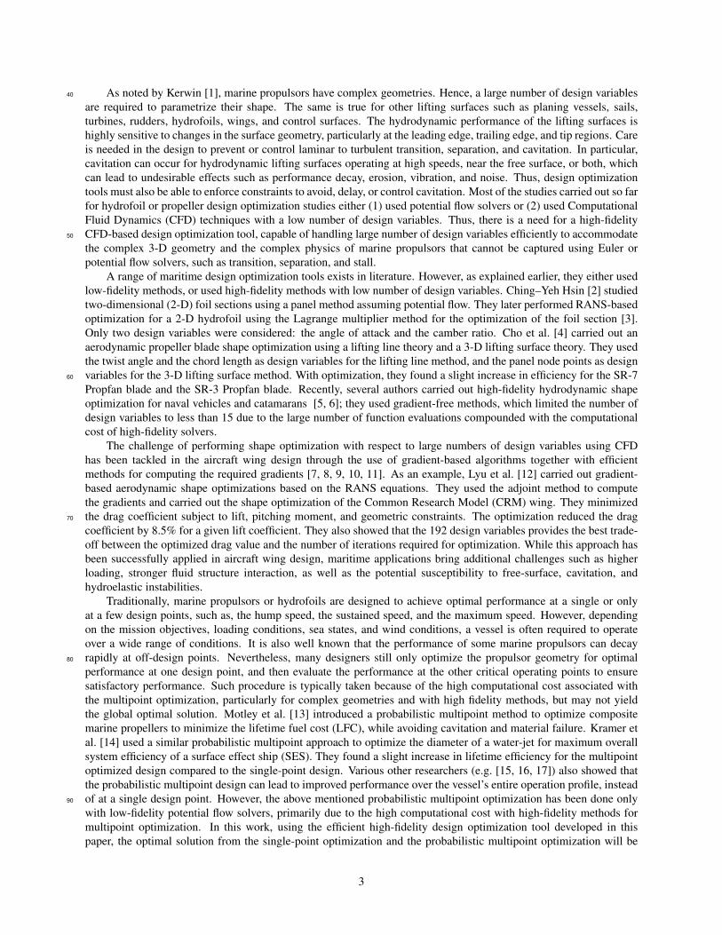
To investigate how the optimal geometry changes with the design CL, the single-point optimization were carried390

out for eachCL. To demonstrate the case at the highest designCL, Figure 8 shows a detailed comparison of the taperedNACA 0009 hydrofoil and the optimized hydrofoil at a CL of 0.75. As shown in Figure 8ii, the spanwise sectionallift distribution for the optimized foil is much closer to the ideal elliptical distribution. The gradient of the sectionallift distribution is also reduced near the tip region for the optimized foil, which translates to reduction in the strengthof the tip vortex. The maximum negative pressure coefficient, �Cp, reduces from 3.1 for the NACA 0009 hydrofoilto 1.2 for the optimized foil, as shown in Figure 8iii, which will help to significantly delay cavitation inception. Inorder words, cavitation inception speed for the optimized foil will increase from 8.4 m/s to 13.50 m/s, for an assumedsubmergence depth of 1 m. The results indicate that partial leading edge cavitation (as indicated by the white contourregion with �Cp ¥ σ) will develop around the original NACA 0009 hydrofoil at CL � 0.75 and σ � 1.6, but nocavitation is observed for the optimized foil. As observed from Figure 8iii, the optimized foil has a higher camber400

and a non-zero spanwise twist/pitch distribution compared to the original NACA 0009 hydrofoil, which reduced theeffective angle of attack and shifted the loading more towards the mid-chord of the foil.

Figure 8: Figure showing single-point optimization result for a tapered NACA 0009 hydrofoil at CL � 0.75, Re � 1.0 � 106, and M � 0.05.A reduction in CD of 14.4% is noted for the optimized foil. Going from top to bottom and from left to right. i) Cp (pressure coefficient) contoursplot on the suction side are displayed for NACA 0009 hydrofoil and the optimized foil. White lines along the span of the hydrofoil show the sectionwhere the �Cp plots and sectional geometry are compared in the plots shown on the right. White contour region along the leading edge of thetapered NACA 0009 foil shows the area with �Cp ¥ σ. ii) Comparative study of the normalized sectional lift distribution with the ideal ellipticallift distribution for the original foil (on the left side) and for the optimized foil (on the right side). There is reduction in the gradient at the tip regionfor the optimized foil, which also results in reduced tip vortex strength. iii) Figures show the sectional �Cp plots and the geometry profile of thefoil at 4 sections along the span of the hydrofoil, the section locations are define in i). Grey solid line represents the NACA 0009 hydrofoil and theblack solid line corresponds to the optimized foil. Black horizontal line represents the constraint on cavitation number. As noted, there is significantdecrease in maximum�Cp from the NACA 0009 to the optimized hydrofoil. Difference in the sectional shape between the original and optimizedfoil are also shown in the bottom of each subplot.

Figure 9 shows the comparison of efficiency (i.e. CL{CD) at the various design CL values for the NACA 0009hydrofoil, the single-point optimized foil at each CL value, and the single-point optimized foil at CL � 0.75 only. Itshould be noted that the single-point optimized foil at each CL requires a different geometry at each CL (as shown inFigure 10), thus it can only be achieved if there is a robust active morphing capability. Assuming that there is an activemorphing capability, with the single-point optimization at each CL value, the best possible performance is achieved;there is a minimum increase in efficiency of 6.4% throughout the operating regime, and the increase in efficiency is19% at theCL value of 0.75, over the original NACA 009 hydrofoil. With the single-point optimized foil atCL � 0.75

16

only, due to fixed geometry; degraded performance was noted when operating away from CL � 0.75; in particular, at410

CL � 0.3, the single-point optimized foil for CL � 0.75 only resulted in a higher CD value than the original NACA0009 hydrofoil. Thus, the results show that, unless there is a robust active morphing capability available, there is aneed for the multipoint optimization to achieve a globally optimal design using one fixed geometry, as demonstratednext in Section 4.4.

15

17

19

21

0.25 0.35 0.45 0.55 0.65 0.75

CL/CD

CL

NACA 0009

Single-point at each C_L

Single-point at C_L = 0.75 only

Figure 9: Figure showing the comparison of efficiency (i.e. CL{CD) versus CL for the tapered NACA 0009 hydrofoil with the single-pointoptimized foil at each CL, and the single-point optimized foil at CL � 0.75 only. All the results were obtained using RANS solver withRe � 1.0� 106 and M � 0.05.

Figure 10: Figure showing the comparison of 3-D geometry between the original tapered NACA 0009 foil, the single-point optimized foil atCL � 0.30, the single-point optimized foil at CL � 0.50, and the single-point optimized foil at CL � 0.75. The RANS-based optimization werecarried out at Re � 1.0� 106 and M � 0.05.

4.4. Comparison of multipoint Optimization and Single-point Optimization

As shown in Section 4.3, the single-point optimization does not necessary result in a globally optimal solutionwith the best efficiency possible over the entire range of operating conditions. The design optimized for CL � 0.75lead to a higher CD than the original foil at CL � 0.3. Such a design would lead to low overall efficiency, particularlyif the probability of operating at CL � 0.75 is low. Hence, a probabilistic multipoint optimization study is needed.

17

For the probabilistic multipoint optimization problem, the objective function (Πobj) is adapted as,420

Πobj �K

m�1

CDmPm (15)

where CDm is the drag coefficient at point m; Pm is the probability of operating at point m; and K is the number ofdesign CL points.

To compare the difference between a single-point and a probabilistic multipoint optimization, a simple threepoint probability distribution, as shown in Table 7, was chosen. The objective function is to minimize the sum ofthe drag coefficient at the three target CL values weighted by the probability of operating at the particular CL value,as shown in Eq. 15. The cavitation number (σ) was fixed at 1.6. The problem setup remains same as shown inSection 3.5. However, to make sure that the problem is well-posed, the angle of attack (define with respect to theoriginal undeformed FFD volume) for CL � 0.75 was fixed at 9.50o, and the angle of attacks for the other CL valuesin the multipoint problem are allowed to be design variables. The multipoint optimization took 2410 processor hours(distributed over 192 processors, 2.60 GHz Intel Xeon E5-2680V2) on the University of Michigan HPC flux cluster.430

Table 7: The simple probabilistic multipoint profile used in the current example.

CL Weights/Probability0.30 0.150.50 0.250.75 0.60

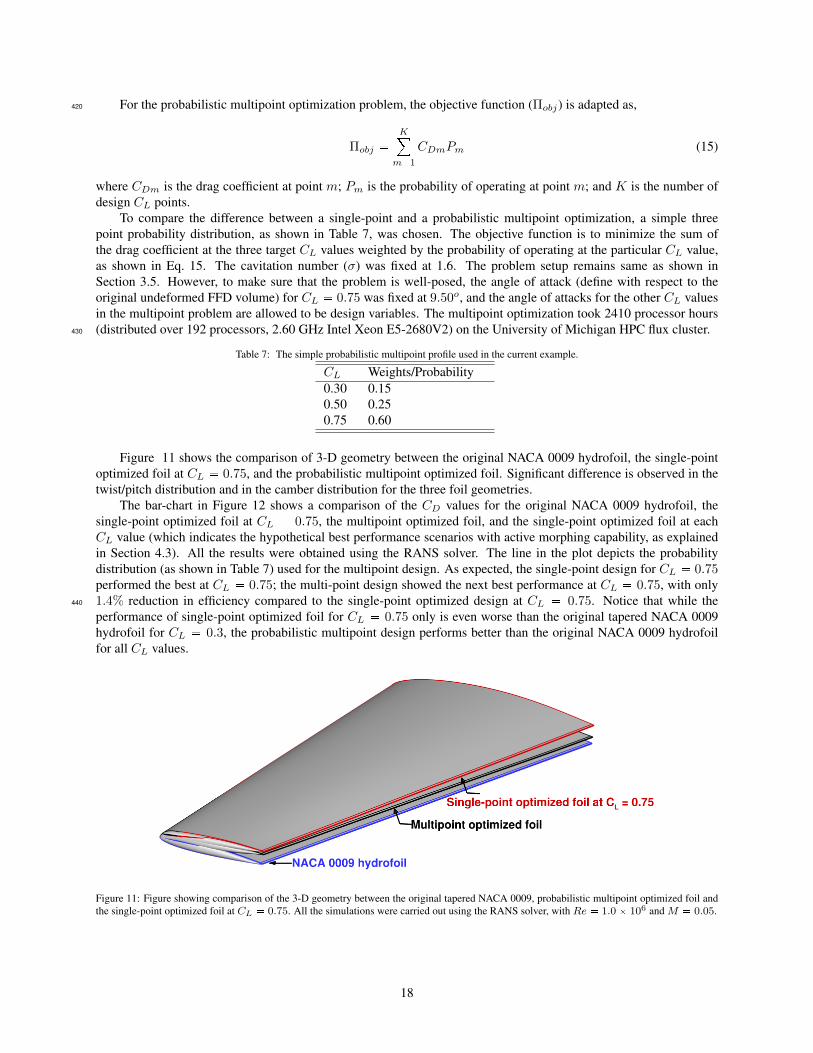
Figure 11 shows the comparison of 3-D geometry between the original NACA 0009 hydrofoil, the single-pointoptimized foil at CL � 0.75, and the probabilistic multipoint optimized foil. Significant difference is observed in thetwist/pitch distribution and in the camber distribution for the three foil geometries.

The bar-chart in Figure 12 shows a comparison of the CD values for the original NACA 0009 hydrofoil, thesingle-point optimized foil at CL � 0.75, the multipoint optimized foil, and the single-point optimized foil at eachCL value (which indicates the hypothetical best performance scenarios with active morphing capability, as explainedin Section 4.3). All the results were obtained using the RANS solver. The line in the plot depicts the probabilitydistribution (as shown in Table 7) used for the multipoint design. As expected, the single-point design for CL � 0.75performed the best at CL � 0.75; the multi-point design showed the next best performance at CL � 0.75, with only1.4% reduction in efficiency compared to the single-point optimized design at CL � 0.75. Notice that while the440

performance of single-point optimized foil for CL � 0.75 only is even worse than the original tapered NACA 0009hydrofoil for CL � 0.3, the probabilistic multipoint design performs better than the original NACA 0009 hydrofoilfor all CL values.

Figure 11: Figure showing comparison of the 3-D geometry between the original tapered NACA 0009, probabilistic multipoint optimized foil andthe single-point optimized foil at CL � 0.75. All the simulations were carried out using the RANS solver, with Re � 1.0� 106 and M � 0.05.

18

0

0.1

0.2

0.3

0.4

0.5

0.6

0.7

0

0.01

0.02

0.03

0.04

0.05

0.3 0.5 0.75

NACA 0009 Single-point at C_L =0.75 Multipoint Single-point at each C_L Probability dist.

CL

CD

Pro

bab

ility

dis

t.

Figure 12: The comparison of CD at different CL values of 0.3, 0.5, and 0.75 for the original tapered NACA 0009 hydrofoil, single-pointoptimized foil at CL � 0.75 only, probabilistic multipoint optimized foil with fixed geometry, and single-point optimized foil at each CL, withvarying geometry at each CL. All the results are obtained using the RANS solver with Re � 1.0 � 106 and M � 0.05. The line depicts theprobability distribution (as shown in Table 7) used for the multipoint optimization problem.

A comparison of the detailed performance of the original tapered NACA 0009 hydrofoil, the single-point opti-mization at CL = 0.75, and the probabilistic multipoint optimization is shown in Figure 13. Columns 2–4 in Figure 13shows the predicted Cp contours for the foils at the CL values specified in the first column. The last column in Fig-ure 13 shows the difference in geometry for the original NACA 0009 hydrofoil, the single-point optimized foil, andthe multipoint optimized foil at Z{S � 0.5. The maximum negative pressure coefficient, �Cp, reduces from 2.9and 3.1 for the NACA 0009 hydrofoil to 1.3 and 1.5 for the multipoint optimized foil, at CL � 0.5 and CL � 0.75,respectively. As noted from Figure 13 Column 2–4, partial leading edge cavitation will develop around the NACA450

0009 hydrofoil for CL ¥ 0.5 and σ � 1.6, but no cavitation is observed for both the optimized foils (the single-point optimized foil and the multipoint optimized foil). Notice that the single-point optimized foil at CL=0.75 has amuch higher camber and a more negative pitch/twist compared to the original foil and the multipoint design; hencethe single-point optimized foil at CL � 0.75 behaves poorly at the lower CL values. As CL = 0.75 has the highestprobability/weight in the probabilistic multipoint optimization, the performance of the multipoint optimized foil andsingle-point optimized foil at design CL of 0.75 is almost same with respect to CD values. However, at other CLpoints in the multipoint optimization, the multipoint design showed better performance, which is expected.

The results show, while the single-point optimization can achieve the best efficiency at the design CL, the single-point optimized foil showed reduced performance at the off-design conditions, namely, CL � 0.3 andCL � 0.5. If theoverall efficiency is calculated as the sum of the efficiency at each CL value multiplied by the probability of operating460

at each CL, the probabilistic multipoint optimized foil will result in overall increase in the efficiency by around 14.4%over the original NACA 0009 hydrofoil. It should be noted that the overall efficiency of the multipoint design (with afixed geometry) is only 1.5% less than the best possible solution from the hypothetical morphing foil (i.e. with varyinggeometry at each CL). The increase in the cavitation inception speed compared to the original NACA 0009 foil, is49% at CL � 0.50, and 39% at CL � 0.75, for an assumed submergence depth of 1 m. This improvement in overallefficiency would be even more obvious if the probability of operating at the highest CL is lower, which is often thecase for many marine propulsors as they seldom operate at the highest loading condition. Thus, it is necessary to carryout the probabilistic multipoint optimization, using realistic mission/operation profiles at an intermediate design stageto achieve a design that performs well throughout the entire range of operating conditions.

19

Figu

re13

:Fig

ure

show

ing

the

com

pari

son

ofth

eor

igin

alN

AC

A00

09hy

drof

oil,

the

sing

le-p

oint

optim

ized

foil

atC

L�

0.75

,and

mul

tipoi

ntop

timiz

edfo

il.A

llth

ere

sults

are

obta

ined

usin

gth

eR

AN

Sso

lver

withRe�

1.0�

106

andM�

0.05

.Col

umns

2–4

show

sth

epr

edic

tedC

pco

ntou

rsfo

rthe

foils

atth

eC

Lva

lues

spec

ified

inth

efir

stco

lum

n.T

hela

stco

lum

nsh

ows

the

diff

eren

cein

geom

etry

fort

heor

igin

alN

AC

A00

09hy

drof

oil,

the

sing

le-p

oint

optim

ized

foil

and

the

mul

tipoi

ntop

timiz

edfo

ilatZ{S�

0.5

.Not

ice

the

whi

teco

ntou

rreg

ion

alon

gth

ele

adin

ged

gefo

rthe

orig

inal

NA

CA

0009

hydr

ofoi

lind

icat

esth

ere

gion

with�C

p¥σ

.N

ote

that

the

figur

esin

the

last

colu

mn

are

notp

lotte

dto

scal

e,to

show

the

diff

eren

cein

geom

etri

esm

ore

prom

inen

tly.

Itca

nbe

obse

rved

from

theC

D

valu

esth

atw

hile

the

sing

le-p

oint

optim

ized

foil

only

perf

orm

sw

ella

tthe

optim

ized

poin

tand

perf

orm

spo

orly

atth

eof

f-de

sign

poin

t,w

hile

the

prob

abili

stic

mul

tipoi

ntop

timiz

edde

sign

perf

orm

sov

erth

een

tire

rang

eof

oper

atin

gco

nditi

ons.

20

5. Conclusions470

In the present work, a low-speed (LS) preconditioner was implemented in an existing compressible CFD solver,SUMad, to solve problems involving nearly incompressible flows for Mach numbers as low as 0.01. The LS SUMadRANS solver was validated against experimental data [25] and verified against commercial CFD software results forthe case of a tapered stainless steel NACA 0009 hydrofoil. The LS SUMad, over predicts theCD values by 14.37% andCL values are under-predicted by 3.3%, when compared with experimental results [25]. However, when LS SUMadresults were compared with commercial CFD software (ANSYS CFX), the average difference was 2.9% in CL and1.7% in CD values, inspite of the different turbulent models.

A design constraint on the cavitation number was developed to optimize the foil to avoid or delay cavitation. Thedevelopment of this cavitation constraint coupled with the adjoint-based optimization algorithm resulted in an efficientand high-fidelity hydrodynamic shape optimization tool for the 3-D lifting surfaces operating under water. To provide480

a canonical representation of a general hydrodynamic lifting surface, the RANS-based optimization results using theadjoint method were presented for an unswept, tapered NACA 0009 hydrofoil at Re � 1.0� 106 and M � 0.05.

The effect of the number of shape design variables was studied in detail. It was found that while the change in CDvalues was not significant, the pressure distribution and geometry varied significantly with the number of shape designvariables. For the hydrofoil considered in this study, a minimum of 203 design variables (200 FFD control points and3 twist variables) was needed to achieve an acceptable optimal solution.

The need for RANS-based design optimization as opposed to Euler-based design optimization was demonstrated.This was evidenced by the fact that 1) the RANS-based and Euler-based design optimizations for the same CL leadto significantly different geometry, and 2) the RANS analysis of the Euler-based optimized foil showed that it cannotdeliver the required lift unless the angle of attack is increased; moreover, to deliver the same CL, RANS-analysis of490

the Euler-based optimized foil will lead to a 11.7% higher drag coefficient, compared to the RANS-optimized foil.To demonstrate the power of the RANS-based shape optimization methodology, a series of optimizations were

performed for the tapered hydrofoil. A single-point optimization was conducted at each CL value with 210 designvariables, where the optimized geometry was significantly different for each CL, and hence a robust active morphingmethod would be needed to realize this design. Nevertheless, such an actively morphed foil would lead to at leastan increase in efficiency of 6.4% throughout the operating profile, and the increase in efficiency would increase to19% for CL � 0.75. The optimized foil at CL � 0.75, would also lead to an increase in the cavitation inceptionspeed by 60%, compared to the original NACA 0009 hydrofoil. However, performance of single-point optimizedfoil degraded when operated away from the design CL value. In particular, the foil optimized for the highest liftcoefficient (CL � 0.75) showed inferior performance even when compared to the original foil at the lowest lift500

coefficient (CL � 0.3) condition.To overcome the issue of degraded performance of the single-point optimized design at the off-design conditions,

a multipoint optimization was carried out. The multipoint optimization was found to perform better than the originalNACA 0009 hydrofoil over the entire operation profile, where the overall efficiency weighted by the probability ofoperation at eachCL, was improved by 14.4% compared to the original NACA 0009 foil. The increase in the cavitationinception speed compared to the original NACA 0009 foil, was 49% at CL � 0.50 and 39% at CL � 0.75, for anassumed submergence depth of 1 m. For the multipoint optimized foil, the geometry remains fixed through out theoperation range and the overall efficiency was only 1.5% less than the hypothetical actively morphed foil with theoptimal geometry at each CL. The results show that the proposed high-fidelity optimization tool can be used tocarry out the probabilistic multipoint optimization, using realistic operation profiles at an intermediate design stage to510

achieve a design that performs well throughout the entire range of operating conditions.Thus, a thorough study of the design space of marine propulsors using the presented high-fidelity multipoint

optimization methodology has the potential to dramatically improve fuel efficiency, agility, and performance over awide range of operating conditions, including extreme off-design conditions (such as crash-stop maneuvers, hard turns,and maneuvering), while at the same time delaying cavitation inception.

6. Future work

The purpose of this paper is to introduce an efficient high-fidelity hydrodynamic shape design optimization tool,capable of handling a large number of design variables over a wide range of operating conditions. In this paper, atapered NACA 0009 hydrofoil is presented as a canonical representation of more complex geometries such as marinepropellers. The capability of handling large number of design variables should be highly beneficial when designing520

21

much more complex geometries and different material configurations, such as those of composite marine propellersand hulls. An efficient high-fidelity solver will also give the freedom to carry out probabilistic multipoint optimizationstudies. Such high-fidelity tool is needed at extreme off-design conditions (e.g., crash-stop maneuvers), where thesolution is governed by separated flow and the large scale vortices. Using the current tool, the optimal design overthe entire range of operating conditions can help designers to achieve the ever increasing minimum energy efficiencylevel per capacity mile, as required by Energy Efficiency Design Index (EEDI), and also to reduce the operatingcosts of the marine vessels. Future work should also include hydrostructural optimization, which would optimizenot only the shape, but also the material configuration of the marine propulsors, hydrofoils or hulls, similarly towhat has already been done for aircraft wings [39, 40, 27]. With hydrostructural design optimization, designer cancontrol and tailor the fluid structure interaction response and reduce the structural weight while ensuring structural530

integrity. Potential examples where hydrostructural optimization can be critical include composite propulsors andturbines, where the load-dependent transformations can be tailored to reduce dynamic load variations, delay cavitationinception, and improve fuel efficiency by adjusting the blade or foil shape in off-design conditions or in spatiallyvarying flow [41, 42].

Acknowledgements

The computations were performed on the Flux HPC cluster at the University of Michigan Center of AdvancedComputing.

Support for this research was provided by the U.S. Office of Naval Research (Contract N00014–13–1–0763),managed by Ms. Kelly Cooper.

References540

[1] J. E. Kerwin, Marine propellers, Annual review of fluid mechanics 18 (1) (1986) 367–403.

[2] C. Y. Hsin, Application of the panel method to the design of two-dimensional foil sections, Journal of Chinesesociety of Naval Architects and Marine Engineers 13 (1994) 1–11.

[3] C. Y. Hsin, J. L. Wu, S. F. Chang, Design and optimization method for a two-dimensional hydrofoil, Journal ofHydrodynamics 18(3) (2006) 323–329.

[4] J. Cho, S.-C. Lee, Propeller blade shape optimization for efficiency improvement, Computers & fluids 27 (3)(1998) 407–419.

[5] W. Wilson, J. Gorski, M. Kandasamy, H. Takai, T., F. W., Stern, Y. Tahara, Hydrodynamic shape optimization fornaval vehicles, High Performance Computing Modernization Program Users Group Conference (HPCMP-UGC)(2010) 161–168.550

[6] E. Campana, D. Peri, Y. Tahara, M. Kandasamy, F. Stern, C.Cary, R. Hoffman, J. Gorski, C. Kennell, Simulation-based design of fast multihull ships, 26th Symposium on Naval Hydrodynamics, September 17–22.

[7] A. Jameson, Computational aerodynamics for aircraft design, Science 245 (1989) 361–371.

[8] W. K. Anderson, V. Venkatakrishnan, Aerodynamic design optimization on unstructured grids with a continuousadjoint formulation, Computers and Fluids 28 (4) (1999) 443–480.

[9] J. J. Reuther, A. Jameson, J. J. Alonso, M. J. Rimlinger, D. Saunders, Constrained multipoint aerodynamic shapeoptimization using an adjoint formulation and parallel computers, part 1, Journal of Aircraft 36 (1) (1999) 51–60.

[10] J. J. Reuther, A. Jameson, J. J. Alonso, M. J. Rimlinger, D. Saunders, Constrained multipoint aerodynamic shapeoptimization using an adjoint formulation and parallel computers, part 2, Journal of Aircraft 36 (1) (1999) 61–74.

[11] J. E. V. Peter, R. P. Dwight, Numerical sensitivity analysis for aerodynamic optimization: A survey of approaches,560

Computers and Fluids 39 (2010) 373–391. doi:10.1016/j.compfluid.2009.09.013.

[12] Z. Lyu, G. K. Kenway, J. R. R. A. Martins, Aerodynamic shape optimization studies on the Common ResearchModel wing benchmark, AIAA Journal 53 (4) (2015) 968–985. doi:10.2514/1.J053318.

22

[13] M. R. Motley, M. Nelson, Y. L. Young, Integrated probabilistic design of marine propulsors to minimize lifetimefuel consumption, Ocean Engineering 45 (2012) 1–8.

[14] M. R. Kramer, M. R. Motley, Y. L. Young, An integrated probability-based propulsor-hull matching methodology,Journal of Offshore Mechanics and Arctic Engineering 135 (1) (2013) 011801.

[15] M. Nelson, D. W. Temple, J. T. Hwang, Y. L. Young, J. R. R. A. Martins, M. Collette, Simultaneous optimizationof propeller–hull systems to minimize lifetime fuel consumption, Applied Ocean Research 43 (2013) 46–52.

[16] Y. L. Young, J. W. Baker, M. R. Motley, Reliability-based design and optimization of adaptive marine structures,570

Composite structures 92 (2) (2010) 244–253.

[17] M. R. Motley, Y. L. Young, Performance-based design and analysis of flexible composite propulsors, Journal ofFluids and Structures 27 (8) (2011) 1310–1325.

[18] T. Brockett, Minimum pressure envelopes for modified NACA-66 sections with NACA A= 0.8 camber andbuships type 1 and type 2 sections, DTIC Document (1996).

[19] R. Eppler, Y. T. Shen, Wing sections for hydrofoils–Part 1: Symmetrical profiles, Journal of ship research (1979)23 (3).

[20] Y. T. Shen, R. Eppler, Wing sections for hydrofoils–Part 2: Nonsymmetrical profiles, Journal of ship research25 (3) (1981) 191–200.

[21] S. Kinnas, S. Mishima, W. Brewer, Nonlinear analysis of viscous flow around cavitating hydrofoils, in: 20th580

Symposium on Naval Hydrodynamics, 1994, pp. 21–26.

[22] S. Mishima, S. A. Kinnas, A numerical optimization technique applied to the design of two-dimensional cavitat-ing hydrofoil sections, Journal of Ship Research 40(1) (1996) 28–38.

[23] Non-linear analysis of the flow around partially or super-cavitating hydrofoils by a potential based panel method.

[24] Z. B. ZENG, G. Kuiper, Blade section design of marine propellers with maximum cavitation inception speed,Journal of Hydrodynamics 24(1) (2011) 65–75.

[25] Z. G.A., P. Brandner, B. Pearce, A. W. Phillips, Experimental study of the steady fluid-structure interaction offlexible hydrofoils, Journal of Fluids and Structure 51 (2014) 326–343.

[26] G. K. W. Kenway, G. J. Kennedy, J. R. R. A. Martins, Scalable parallel approach for high-fidelity steady-stateaeroelastic analysis and derivative computations, AIAA Journal 52 (5) (2014) 935–951. doi:10.2514/1.590

J052255.

[27] G. K. W. Kenway, J. R. R. A. Martins, Multipoint high-fidelity aerostructural optimization of a transport aircraftconfiguration, Journal of Aircraft 51 (1) (2014) 144–160. doi:10.2514/1.C032150.

[28] E. van der Weide, G. Kalitzin, J. Schluter, J. J. Alonso, Unsteady turbomachinery computations using massivelyparallel platforms, in: Proceedings of the 44th AIAA Aerospace Sciences Meeting and Exhibit, Reno, NV, 2006,AIAA 2006-0421.

[29] Z. Lyu, G. K. Kenway, C. Paige, J. R. R. A. Martins, Automatic differentiation adjoint of the Reynolds-averagedNavier–Stokes equations with a turbulence model, in: 21st AIAA Computational Fluid Dynamics Conference,San Diego, CA, 2013. doi:10.2514/6.2013-2581.

[30] A. Jameson, W. Schmidt, E. Turkel, Numerical solutions of the euler equations by finite volume methods using600

Runge–Kutta time-stepping schemes, AIAA paper (1981) 1259.

[31] P. Spalart, S. Allmaras, A one-equation turbulence model for aerodynamic flows, in: 30th Aerospace SciencesMeeting and Exhibit, 1992. doi:10.2514/6.1992-439.URL http://dx.doi.org/10.2514/6.1992-439

23

[32] E. Turkel, R. Radespiel, N. Kroll, Assessment of preconditioning methods for multidimensional aerodynamics,Computer and Fluids 26(6) (1997) 613–634.

[33] Y. H. Choi, C. L. Merkle, The application of preconditioning in viscous flows, Journal of Computational Physics105(2) (1993) 207–223.

[34] B. Van Leer, W. T. Lee, P. L. Roe, Characteristic time-stepping or local preconditioning of the euler equations,10th Computational Fluid Dynamics Conference 1 (1991) 260–282.610

[35] Z. Lyu, Z. Xu, J. R. R. A. Martins, Benchmarking optimization algorithms for wing aerodynamic design opti-mization, in: 8th International Conference on Computational Fluid Dynamics (ICCFD8), Chengdu, China, 2014,ICCFD8 2014-0203.

[36] J. R. R. A. Martins, P. Sturdza, J. J. Alonso, The complex-step derivative approximation, ACM Transactions onMathematical Software (TOMS) 29(3) (2003) 245–262.

[37] J. R. R. A. Martins, J. T. Hwang, Review and unification of methods for computing derivatives of multidisci-plinary computational models, AIAA Journal 51 (11) (2013) 2582–2599. doi:10.2514/1.J052184.

[38] P. E. Gill, W. Murray, M. A. Saunders, SNOPT: An SQP algorithm for large-scale constrained optimization,SIAM Journal on optimization (2002) 976–1006.

[39] G. K. W. Kenway, J. R. R. A. Martins, Multipoint aerodynamic shape optimization investigations of the Common620

Research Model wing, in: Proceedings of the AIAA Science and Technology Forum and Exposition (SciTech),Kissimmee, FL, 2015, aIAA 2015-0264. doi:10.2514/6.2015-0264.

[40] R. Liem, G. K. W. Kenway, J. R. R. A. Martins, Multimission aircraft fuel burn minimization via multipointaerostructural optimization, AIAA Journal 53 (1) (2015) 104–122. doi:10.2514/1.J052940.

[41] Y. L. Young, Fluid–structure interaction analysis of flexible composite marine propellers, Journal of Fluids andStructures 24 (6) (2008) 799–818.

[42] Y. L. Young, M. R. Motley, R. W. Yeung, Three-dimensional numerical modeling of the transient fluid-structuralinteraction response of tidal turbines, Journal of Offshore Mechanics and Arctic Engineering 132 (1) (2010)011101.

24