http://www.uta.edu/math/preprint/

Technical Report 2007-15

High Order Modified Weighted Compact Scheme for High

Speed Flow

Chaoqun LiuPeng Xie

Maria L. Oliveira

High Order Modified Weighted Compact Scheme for High

Speed Flow

(TECHNICAL REPORT FOR THE 2007 VA SUMMER PROGRAM)

CHAOQUN LIU, PENG XIE & MARIA L OLIVEIRA

UNIVERSITY OF TEXAS AT ARLINGTON, ALRINGTON, TX 76019

CLIU@UTA.EDU

ABSTRACT

The critical problem of CFD is perhaps an accurate approximation of derivatives for a given

discrete data set. Based on our previous work on the weighted compact scheme (WCS), a

modified weighted compact scheme (MWCS) has been developed. Similar to WENO, three high

order candidates, left, right, and central, are constructed by Hermite polynomials. According to

the smoothness, three weights are derived and assigned to each candidate. The weights will lead

the scheme to be bias when approaching the shock or other discontinuities but quickly becomes

central, compact, and of high order just off the shock. Therefore, the new scheme can get a sharp

shock without oscillation, but keep central, compact and of high resolution in the smooth area.

This feature is particularly important to numerical simulation of the shock-boundary layer

interaction, where both shock and small eddies are important. The new scheme has three

compact candidate stencils, 210 ,, EEE , with three weights 210 ,, ωωω . Candidate stencils

210 ,, EEE have third order, fourth order, and third order of accuracy respectively.

Picking18

1,

9

8,

18

1210 === ωωω , MWCS has sixth order of accuracy in the smooth area. For

near shock grid points, 0,0,1 210 === ωωω , MWCS still has fourth order of accuracy.

Comparing with 5th

order WENO which has 5th

order in the smooth area and third order near the

shock, MWCS is super with smaller stencils and higher order of accuracy. The necessary

dissipation is provided by weights and some high order bias up-winding scheme. The new

scheme has been successfully applied for 1-D shock tube and shock-entropy interaction and 2-D

incident shock. The new scheme has obtained sharper shock, no deformation for expansion

wave, and much higher resolution than 5th

order WENO for small length scales. A first version

of a black-box type subroutine with MWCS scheme has been developed and given to AFRL

collaborators. The subroutine can give a high order derivative for any discrete data sets, no

matter they are smooth, highly oscillatory, or no-differentiable. The scheme is currently applied

for shock-boundary layer interaction with double cones for validation. A variety of cases

including shock-boundary interaction with incident shock, double angles and double-cones is

being tested.

The preliminary numerical solution is encouraging while the numerical simulation with double

angles and double cones are still running. The new effort will also focus on new versions of the

black-box type subroutines. The first version requires explicit boundary values. The second

version will be able to treat variety of boundary conditions implicitly and keep high order for the

boundary points. The third and fourth version will include fast computation and self flux

splitting.

1. Introduction

1.1 A short overview on shock capturing schemes

The flow filed is in general governed by the Navier-Stokes system which is a system of time

dependent partial differential equations. However, for external flow, the viscosity is important

largely only in the boundary layers. The main flow can still be considered as inviscid and the

governing system can be dominated by the time dependent Euler equations which are hyperbolic.

The difficult problem with numerical solution is the shock capturing which can be considered as

a discontinuity or mathematical singularity (no classical unique solution and no bounded

derivatives). In the shock area, continuity and differentiability of the governing Euler equations

are lost and only the weak solution in an integration form can be obtained. The shock can be

developed in some cases because the Euler equation is non-linear and hyperbolic. On the other

hand, the governing Navier-Stokes system presents parabolic type behavior in and is therefore

dominated by viscosity or second order derivatives. One expects that the equation should be

solved by high order central difference scheme, high order compact scheme is preferable, to get

high order accuracy and high resolution. High order of accuracy is critical in resolving small

length scale in flow transition and turbulence process. However, for the hyperbolic system, the

analysis already shows the existence of characteristic lines and Riemann invariants. Apparently,

the upwind finite difference scheme coincides with the physics for a hyperbolic system. History

has shown the great success of upwind technologies. We should consider not only the

eigenvalues and eigenvectors of the Jacobian system, but also non-linearity including the

Rankine-Hugoniot shock relations. From the point of view of shocks, it makes no sense to use

high order compact scheme for shock capturing which use all gird points on one grid line to

calculate the derivative by solving a tri-diagonal or penta-diagonal linear system when shock

does not have finite derivatives and downstream quantities cannot cross shock to affect the

upstream points. From the point of view of the above statement, upwind scheme is appropriate

for the hyperbolic system. Many upwind or bias upwind schemes have achieved great success in

capturing the shocks sharply, such as Godnov (1959), Roe (1981), MUSCL (Van Leer, 1979),

TVD (Harten, 1983), ENO (Harten et al, 1987; Shu et al, 1988, 1989) and WENO (Liu et al,

1994; Jiang et al, 1996). Roe’s scheme may be better in capturing the shock sharply because it

satisfies the Rankine-Hugoniot relation. Of course, Roe’s method can also be considered as a

method for flux difference splitting and any high order method such as ENO and WENO can use

Roe’s method as a splitting method. However, all these shock-capturing schemes are based on

upwind or bias upwind technology, which is nice for hyperbolic system, but is not favorable to

the N-S system which presents parabolic equation behavior. The small length scale is very

important in the flow transition and turbulence process and thus very sensitive to any artificial

numerical dissipation. High order compact scheme (Lele, 1992; Visble, 2002) is more

appropriate for simulation of flow transition and turbulence because it is central and non-

dissipative with high order accuracy and high resolution.

Unfortunately, the shock-boundary layer interaction, which is important to high speed flow, is a

mixed type problem which has shock (discontinuity), boundary layer (viscosity), separation,

transition, expansion fans, fully developed turbulence, and reattachment. In order to capture the

shock and keep high order accuracy and high resolution in the smooth area, we have developed

the so called weighted compact scheme (WCS, Jiang et al, 2001) which works very well for 1-D

convection equation, Burger’s equation, but not so good for Euler’s equation with shocks.

Visible wiggles have been found near the shock. In the case of shock-boundary layer interaction,

there are elliptic areas (separation, transition, turbulence) and hyperbolic areas (main flow,

shocks, expansion fans), which makes the accurate numerical simulation extremely difficult if

not impossible. We have to divide the computational domain to several parts: the elliptic,

hyperbolic, and mixed. The division or detection can be performed by switch function

automatically such as shock detector which simply sets 1=Ω for the shock area and 0=Ω for

the rest. The switch function may give the best results for shock-boundary layer interaction, but

it will have too many logical statements in the code which may slow down the computation. The

switch function could also be case-related and very difficult to adjust. It would also slow down

the convergence for steady problems. The use of “weights” will be naturally considered as a

good candidate that succeeded for many schemes, WENO is a good example and our Weighted

Compact Scheme is another example.

Traditional finite difference schemes use the idea of Lagrange interpolation. To obtain nth order

of accuracy, a stencil covering n+1 grid points is needed. In other words, the derivative at a

certain grid point depends upon the function values at these n+1 grid points and only these grid

points. In contrast, standard compact schemes (Lele, 1992; Visbal, 2002) use the idea of

Hermitian interpolation. By using derivatives as well as function values, a compact scheme

achieves high order of accuracy without increasing the width of stencils. As discussed in Lele’s

paper, a compact scheme has not only high order of accuracy, but also high resolution. Fourier

analysis indicates that, with the same order of accuracy, a compact scheme has better spectral

resolution than a traditional, explicit finite difference scheme. For this reason, compact schemes

are favorable in the simulation of turbulent flows where small-length-scale structures are

important.

Due to the usage of derivatives, compact schemes usually give us a tri-diagonal or penta-

diagonal system. Although the tri-diagonal matrix is sparse, the inverse of a tri-diagonal matrix is

dense, which means the derivative at a certain grid point depends upon all the grid points along a

grid line. The success of compact schemes indicates that the global dependency is very important

for high resolution. However, the global dependency is good for resolution but not so applicable

for shock capturing.

The basic idea proposed in ENO (Harten et al, 1987) and WENO (Jiang et al, 1996) schemes is

to avoid the stencil containing a shock. ENO chooses the smoothest stencil from several

candidates to calculate the derivatives. WENO controls the contributions of different stencils

according to their smoothness. In this way, the derivative at a certain grid point, especially one

near the shock, is dependent on a very limited number of grid points. The local dependency here

is favorable for shock capturing and helps obtaining the non-oscillatory property. The success of

ENO and WENO schemes indicates that the local dependency is critical for shock capturing.

The Weighted Compact Scheme (WCS) we developed (Jiang et al, 2001) is constructed by

introducing the idea of WENO scheme to the standard compact schemes which uses weights for

several candidates. The building block for each candidate is a Lagrange polynomial in WENO,

but is Hermite in WCS. Therefore WCS achieves a higher accuracy with same stencil width. In

shock regions, WCS controls the contributions of different candidate stencils to minimize the

influence of the candidate which contains a shock. In smooth regions where shocks are not

present, WCS recovers to the standard compact scheme to achieve high accuracy and resolution.

The numerical tests indicate that original WCS works fine in some cases such as convection

equation and Burger’s equation, but not very well for Euler equation. As mentioned above, the

usage of derivatives by compact schemes results in the global dependency.

In order to overcome the drawback of the WCS scheme, we need to achieve local dependency in

shock regions and recover the global dependency in smooth regions. This fundamental idea will

naturally lead to a combination of local dependent scheme, e.g. WENO and global dependent

weighted compact schemes which we call “Modified Weighted Compact Scheme” (MWCS).

The mixing and weights are designed in following ways: the new scheme automatically becomes

bias when approaching the shock, but rapidly recovers to be central, compact, with high order of

accuracy and high resolution. This kind of scheme has been developed and preliminary

computation results are very promising. The new scheme needs to be optimized and validated for

2-D and 3-D cases.

1.2 Importance of high order scheme to DNS/LES

It should be pointed out that the order of accuracy of the finite difference scheme is

absolutely not a trivial issue to CFD, especially to DNS and LES. There is a significant

difference in requirements of grid size by DNS/LES between low order schemes and high order

schemes. Let us take a look at the local truncation error for 1-D problem. If one uses a second

order scheme with a mesh size of 2x∆ and wants to have same truncation error using a sixth order

scheme with a mesh size of 6x∆ , one should have: 6

66

2

22 )()( xCxC ∆=∆ (1.1)

Assume 62 CC ≈ and 01.06 =∆x (100 grid points in a normalized domain), we will get

622

2 )10()( −=∆x

6

2 10−=∆x (1.2)

In other words, the second order scheme needs one million of grid points to beat the sixth order

scheme with 100 grid points for same order of accuracy. This advantage of high order scheme

will become more significant when one uses DNS for 3-D problems. We do not want to use one

million of grids in each direction for DNS, but prefer to use 100 grid points. Therefore high order

scheme must be used. Of course, the global accuracy is also influenced by factors other than the

local truncation errors, and the advantage of the sixth order scheme does not typically show a

magnitude of 10 thousand times improvement over the second order scheme. However, it is now

widely recognized that high order finite schemes are strongly encouraged to be used for DNS

and LES which have much higher accuracy and higher resolution than low order schemes.

1.3 Comments on low order LES with low order subgrid models

Most LES computations require use of a subgrid model trying to get the unresolved scales back,

which could be mathematically considered as truncation errors. Let us take a look at the famous

Smagorinsky model:

ijtij Sντ −= and

||)( 2SCst ∆=ν

(1.3)

Where ∆,,, sijij CSτ are the unresolved stress tensor, resolved strain tensor, Smogorinsky

constant, and filter width respectively. Apparently, it is a second order model with 2∆ . Other

models are similar. If we use a sixth order compact scheme for LES without model (Implicit

LES), we will get sixth order of accuracy. However, if we add the Smgorinsky subgrid model,

our LES results will be degenerated to second order of accuracy, which is really bad. A carefully

designed 6th

order subgrid model may be needed for high order LES. Therefore, second order

DNS, second order LES with second order subgrid models are not appropriate for DNS or LES.

Table 1 shows the orders obtained by different orders of schemes, which demonstrates the

importance of high order numerical schemes for DNS/LES.

Table 1. Orders of DNS/LES approaches

Scheme Truncation Errors Comments

Second order DNS )( 2hO Bad

Second order LES +Second order

subgrid model )( 2hO or up Bad

Sixth order LES without subgrid

model (ILES) )( 6hO Good

Sixth order LES with second order

subgrid model )( 2hO Bad

Sixth order LES with sixth order

subgrid model )( 6hO or up Best

1.4 Basic point of view on the scheme development

The 3-D time dependent Navier-Stokes equations in a general curvilinear coordinate can be

written as

(1.4)

For 1-D conservation law, it will be:

( ) ( ) ( )0

1=

∂

−∂+

∂

−∂+

∂

−∂+

∂

∂

ζηξvvv FFFFEE

t

Q

J

0=∂

∂+

∂

∂

ξ

E

t

Q

(1.5)

The critical issue for high order CFD is to find an accurate approximation of derivatives for a

given discrete data set. The computer does not know any physical process but accepts a discrete

data set as input. The output is also a discrete data set. We measure the input data by slopes to

determine it is smooth (slope is small), oscillatory (slope is large), and non-differentiable (or

corner points which have slopes large on one side, but small on the other side), or, in other

words, by a smoothness function, and then an appropriate numerical scheme is set up based on

the feature of the discrete data set, but not the governing system. This is the basic view point for

our new scheme development.

2. Technical Approach

2.1 ENO reconstruction function

For 1-D conservation laws:

0)),((),( =+ txuftxu xt (2.1)

When a conservative approximation to the spatial derivative is applied, a semi-discrete

conservative form of the equation (2.1) is described as follows:

)ˆˆ(1

)2/1()2/1( −+ −∆

−= jj

jff

xdt

du (2.2)

where ∫∆+

∆−∆=

2/

2/)(ˆ1 xx

xxj

j

j

dfx

f ξξ and then )ˆˆ(1

)( )2/1()2/1( −+ −∆

−= jjjx ffx

f . Note that f is the

original function, but f is the flux defined by the above integration which is an exact

expression of the flux but is different from f.

Let H be the primitive function of f defined below:

∑∫∑∫−∞=

∆+

∆−

=

−∞=

∆+

∞−+ ∆===

j

i

i

xx

xx

ji

i

xx

j fxdfdfxHi

i

j 2/

2/

2/

)2/1( )(ˆ)(ˆ)( ξξξξ (2.3)

H is easy to be calculated, but is a discrete data set.

The numerical flux f at the cell interfaces is the derivative of its primitive function H. i.e.:

'

)2/1()2/1(ˆ

++ = jj Hf (2.4)

All formulae given above are exact without approximations. However, the primitive function H

is a discrete data set or discrete function and we have to use numerical method to get the

derivatives, which will introduce numerical errors, or, in other words, order of accuracy.

This procedure, 'ˆxffHf →→→ , is called reconstruction introduced by Shu & Osher (1988,

1989). There is one and only one problem left for numerical methods, which is how to solve

(2.4) or how to get accurate derivatives for a data set.

2.2 Data normalization

In order to find universal formula, we need to normalize the data set, u(i), i=1, …, n:

|| minmax uuudiff −= (2.5)

diffuuuu /)( min−= (2.6)

Here, maxu and minu are the maximum and minimum values of u respectively and u is

normalized. For simplicity, we throw out the hat of u and use u (i) as the normalized data set.

2.3 Weighted compact scheme

As we addressed that there is one and only one problem left for numerical methods, which is

how to solve (2.4) or how to get accurate derivatives for a discrete data set. It is equivalent to

finding an accurate flux in the interface. We turn our attention into finding a high order scheme

which, however, must be able to pass the shock without non-physical wiggles.

2.3.1 WENO Scheme (Jiang & Su, 1996)

Before discuss our new scheme, first let us see how to construct the WENO scheme.

2.3.1.1 Conservation Form of Derivative

0=∂

∂+

∂

∂

x

F

t

U (2.7)

The ENO reconstruction can provide a semi-discretization for the derivative: x

FF

x

F ii

∆

−

=∂

∂ −+2

1

2

1ˆˆ

,

where F is the flux which must be accurately obtained.

2.3.1.2 5th

Order WENO (bias upwind)

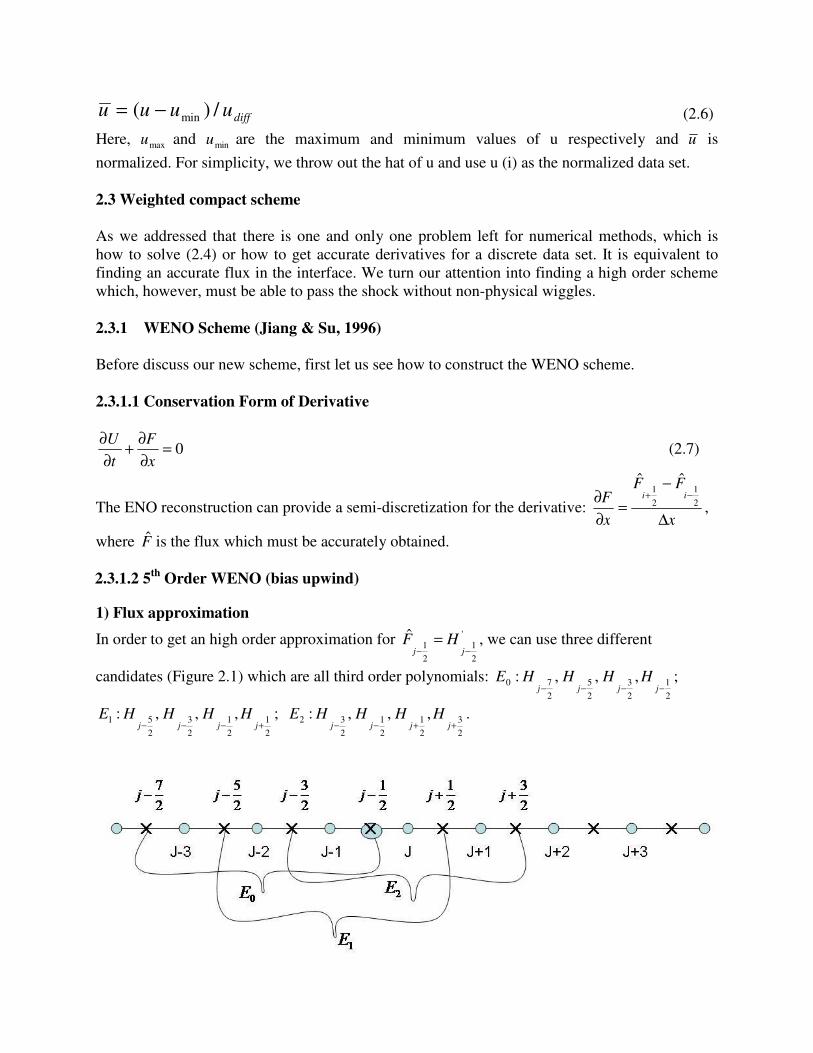
1) Flux approximation

In order to get an high order approximation for '

2

1

2

1ˆ

−−=

jjHF , we can use three different

candidates (Figure 2.1) which are all third order polynomials: 2

1

2

3

2

5

2

70 ,,,:−−−− jjjj

HHHHE ;

2

1

2

1

2

3

2

51 ,,,:+−−− jjjj

HHHHE ; 2

3

2

1

2

1

2

32 ,,,:++−− jjjj

HHHHE .

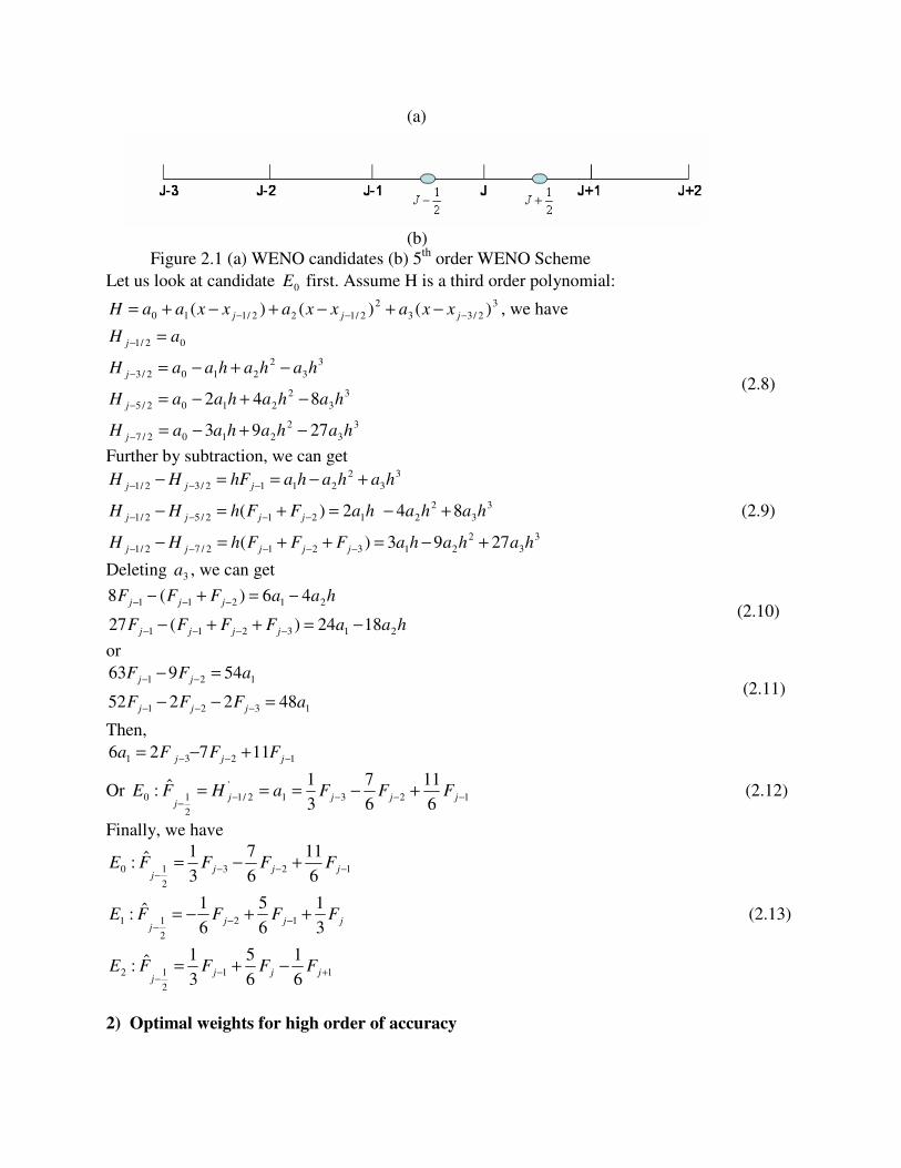
(a)

(b)

Figure 2.1 (a) WENO candidates (b) 5th

order WENO Scheme

Let us look at candidate 0E first. Assume H is a third order polynomial:

3

2/33

2

2/122/110 )()()( −−− −+−+−+= jjj xxaxxaxxaaH , we have

3

3

2

2102/7

3

3

2

2102/5

3

3

2

2102/3

02/1

2793

842

hahahaaH

hahahaaH

hahahaaH

aH

j

j

j

j

−+−=

−+−=

−+−=

=

−

−

−

−

(2.8)

Further by subtraction, we can get

3

3

2

213212/72/1

3

3

2

21212/52/1

3

3

2

2112/32/1

2793)(

842)(

hahahaFFFhHH

hahahaFFhHH

hahahahFHH

jjjjj

jjjj

jjj

+−=++=−

+−=+=−

+−==−

−−−−−

−−−−

−−−

(2.9)

Deleting 3a , we can get

haaFFFF

haaFFF

jjjj

jjj

213211

21211

1824)(27

46)(8

−=++−

−=+−

−−−−

−−− (2.10)

or

1321

121

482252

54963

aFFF

aFF

jjj

jj

=−−

=−

−−−

−− (2.11)

Then,

1231 11726 −−− +−= jjj FFFa

Or 1231

'

2/1

2

106

11

6

7

3

1ˆ: −−−−−

+−=== jjjjj

FFFaHFE (2.12)

Finally, we have

123

2

106

11

6

7

3

1ˆ: −−−−

+−= jjjj

FFFFE

jjjj

FFFFE3

1

6

5

6

1ˆ: 12

2

11 ++−= −−−

(2.13)

11

2

126

1

6

5

3

1ˆ: +−−

−+= jjjj

FFFFE

2) Optimal weights for high order of accuracy

The final scheme should be a combination of three candidates: 221100 ECECECE ++=

If we set10

3,

10

6,

10

1210 === CCC , we will have

1123

2

120

1

60

27

60

47

60

13

30

1ˆ+−−−

−−++−= jjjjj

jFFFFFF

2112

2

120

1

60

27

60

47

60

13

30

1ˆ++−−

+−++−= jjjjj

jFFFFFF (2.14)

)(/)20

1

2

1

3

1

4

1

30

1(

ˆˆ

5

211232

1

2

1

xOxFFFFFFx

FF

x

Fjjjjjj

jj

∆+∆−++−+−=∆

−

=∂

∂++−−−

=+

Using Taylor expansion for kjF − , we find

( ) ( ) ( ) ( ) ...'

ˆˆ

++−=

−

=∂

∂ −+76652

1

2

1

140

1

60

1jjj

jj

FxFxFx

FF

x

F∆∆

∆, (2.15)

which shows the scheme with optimal weights and 6 grid points has a 5th

order truncation error.

Note that the scheme is a STANDARD 5th

order bias upwind finite difference scheme.

3) Bias up-wind weights:

Let us define a bias weight for each candidate according to WENO:

∑ =

=2

0i i

kk

γ

γω ,

p

k

kk

IS

C

)( +=

εγ (2.16)

where

∫ ∑+

−

−∞

=

=2/1

2/1

122)(

2

1

])([j

j

x

x

kk

k

i dxhxpIS

2

12

2

120 )34(4

1)2(

12

13jjjjjj FFFFFFIS +−++−= −−−−

2

11

2

111 )(4

1)2(

12

13+−+− −++−= jjjjj FFFFFIS

2

12

2

212 )34(4

1)2(

12

13jjjjjj FFFFFFIS +−++−= ++++

The 5th

order WENO can be obtained

2211002/1ˆ EEEF j ωωω ++=− (2.17)

)6

1

6

5

3

1(

)3

1

6

5

6

1()

6

11

6

7

3

1(ˆ

112/1,2

122/1,11232/1,02/1

+−−

−−−−−−−−

−++

++−++−=

jjjj

jjjjjjjjj

FFF

FFFFFFF

ω

ωω (2.18)

WENO is a great scheme with great successes by many users. However, the scheme has 5th

order

dissipation everywhere and third order dissipation near the shock and people in DNS/LES

community complain it is too dissipative for transition and turbulence. Let us turn into central

and compact schemes for assistance.

2.3.2 Weighted Compact Scheme (WCS, Jiang et al, 2001)

1) High-order compact schemes

A Pade-type compact scheme could be constructed based on the Hermite interpolation where

both function and derivatives at grid points are involved, e.g. a fourth order finite difference

scheme can be constructed if both the function and first order derivative are used at three grid

points. For a function f we may write a compact scheme by using five grid points (Lele, 1992):

ξβααβ ∆++++=++++ ++++−−−−++++−−−− /)( 2112

'

2

'

1

''

1

'

2 jjjjjjjjjj fbfacffafbfffff (2.19)

We can get 8th

order of accuracy by using the above formula based on Taylor series.

If we use a symmetric and tri-diagonal system, by setting 0== +− ββ , we can get a one

parameter family of compact scheme (Lele, 1992):

( ) ( ) ( ) ( ) hfffffff ijjii ii/14

12

12

3

12

3

114

12

12112

'''

11

−++++−−−=++ ++−−+−

αααααα (2.20)

If 31=α , we will get a standard sixth order compact scheme.

When a compact scheme is used to differentiate a discontinuous or shock function, the computed

derivative has grid to grid oscillations. In our previous work (Jiang et al, 2001) we proposed a

new class of finite difference scheme - weighted compact scheme (WCS).

2) Basic formulations of weighted compact scheme

(a)

(b) Figure 2.2 (a) WCS Stencil Candidates (b) Sixth Order Compact Scheme

In order to get an high order approximation for '

2

1

2

1ˆ

−−=

jjHF , the six order weighted compact

scheme uses three candidates for 2

1ˆ

−jF as shown in Figure 2.2 (a) which are all polynomials:

2/12/32/50 ,,: −−− jjj HHHE , 2/12/12/31 ,,: +−− jjj HHHE , and 2/32/12/12 ,,: ++− jjj FHHE (2.21)

Note that:

xFHj

i

ij ∆=∑−

=−

1

0

2/1 (2.22)

Compact schemes are used for these three candidates:

xHcHaHbHHE jjjjj ∆+−−=+ −−−−− /)(: 2/102/302/50

'

2/1

'

2/300 α

xHHaHHHE jjjjj ∆−=++ −++−− /)(: 2/32/11

'

2/11

'

2/1

'

2/311 αα (2.23)

xHcHaHbHHE jjjjj ∆−+=+ −+++− /)(: 2/122/122/32

'

2/12

'

2/12 α

For high order, we pick

2

5,

2

5,

2

1,

2

1,2,

4

3,2,2,

4

1,2 2020210210 ========== ccbbaaaααα (2.24)

0E and 2E have third order, but 1E has fourth order of accuracy.

The compact scheme for each candidate is:

0E : 212/12/32/5

'

2/1

'

2/32

1

2

5

2

52

2

12 −−−−−−− +=

+−−=+ jjjjjjj FFhHHHHH

1E : ( )

)(4

3

4

3

4

1

4

11

2/32/1'

2/1

'

2/1

'

2/3 −

−+

+−− +=−

=++ jj

jj

jjj FFh

HHHHH (2.25)

2E : jjjjjjj FFhHHHHH2

5

2

1

2

52

2

12 12/12/12/3

'

2/1

'

2/1 +=

−+=+ +−+++−

3) Non-bias compact scheme

Let 221100 ECECECE ++= and 18

1,

18

16,

18

1210 === CCC

E: 112

'

2/1

'

2/1

'

2/336

1

36

29

36

29

36

1

3

1

3

1+−−+−− +++=++ jjjjjjj FFFFHHH (2.26)

Similarly, E at point 2/1+j is

211

'

2/3

'

2/1

'

2/136

1

36

29

36

29

36

1

3

1

3

1++−++− +++=++ jjjjjjj FFFFHHH (2.27)

Subtracting the previous equation at point j-1/2, we get

)36

1

9

7

9

7

36

1(

1

3

1

3

12112

'

1

''

1 ++−−+− ++−−=++ jjjjjjj FFFFh

FFF (2.28)

This is a standard sixth order compact scheme. The stencil candidates are 120 ,: −− jj FFE ,

jj FFE ,: 11 − , and 12 ,: +jj FFE for 2/1

'

2/1ˆ

−− = jj FH . This also shows the WCS uses smaller

candidate stencils but gets higher accuracy comparing with the 5th

order WENO.

The procedure described above implies that a sixth order centered compact scheme can be

constructed by a combination of three lower order schemes. In order to achieve the non-

oscillatory property, the WENO weights (Jiang et al., 1996) are introduced to determine new

weights for each stencil. The weights are determined according to the smoothness of the function

on each stencil. Following the WENO method, the new weights are defined as

∑ =

=2

0i i

k

k

γ

γω

p

k

k

kIS

C

)( +=

εγ (2.29)

where ε is a small positive number to prevent the denominator becoming zero and p is a

parameter to control the weighting. Actually, p is very sensitive to affect the weights. We set p as

a function of smoothness instead of constant. When p=0, the 6th

order standard compact scheme

is recovered. ISk is a smoothness measurement which is defined in (2.16). Through the Taylor

expansion, it can be easily proved that in smooth regions the new weights kω satisfy:

)( 2hOCkk +=ω and

)( 3

02 hO=− ωω (2.30)

The new scheme is formed using these new weights:

221100 EEEE ωωω ++= (2.31)

The leading error of E is a combination of the leading errors of the original schemes, which is:

4)5(

210

3)4(

20 )15

1

120

1

15

1()

12

1

12

1( hfhf ωωωωω −+−+− (2.32)

When equation (2.30) is satisfied, the leading error of the new scheme can be written as

)( 6hO and the new scheme remains its 6th

order of accuracy.

2.3.3 Modified Weighted Compact Scheme MWCS)

It seems like the WCS scheme is super over WENO especially for the shock-turbulence

interaction, where both discontinuity and small length scales are important, when it uses Hermite

polynomials as its building block. It is sixth order in the smooth area with weights of

18

1,

9

8,

18

1and 4

th order near the shock with weights of 1, 0, 0. The WCS really obtain pretty good

results for wave equation and Burger equation. However, it is not so favorable for Euler

equation. For 1-D shock tube case, it generates wiggles before and after the shock. For 2-D it

meets more difficulties and blows up frequently. The reason is apparently that the WCS scheme

does not have enough dissipation around the shock , which causes wiggles. Because the scheme

is non-dissipative and central, the wiggles cannot be dissipated after they are generated. Then, a

second order filter is required to remove these wiggles. However, the second order filter is case-

related and has adjustable constants. There is always a risk to reduce the order of calculation by

using second order filter. In this consideration, we tried to modify the flux given by (2.33):

biaswcsmwcs FxFxF ))(1()( αα −+= (2.33)

The bias flux can be obtained by up-wind or bias up-wind schemes and only play roles near the

shock (corner points). For the purpose to keep high order, we use the 5th

order WENO in current

work as a flux modification. The advantage is that WCS and WENO can share the smoothness

measurement and WENO has 5th

order accuracy. From computational practice, WENO looks too

dissipative inside the boundary layers, but not strong enough to capture the shock without

oscillation. We really need to find a better and optimized modification by choosing new )(xα and

biasF

2.3.4 Comparison of WENO and MWCS

2.3.4.1 Comparison in computation

1) Shock tube

Let first take a shock tube problem to see how the WENO works. The governing equations are

1D Euler equations:

0=∂

∂+

∂

∂

x

F

t

U (2.34)

( )TEuU ,, ρρ= ; ( )( )T

pEupuuuF ++= ,, ρρ

The initial conditions are given as follows:

( )( )( )

≥

<=

.01.0,0,125.0

;0,1,0,1,,

x

xpuρ (2.35)

To solve the Euler equations, Three step TVD Runge-Kutta is used in time marching and Lax-

Friedrich flux vector splitting is used and the derivatives of splitting flux +F , −F are calculated

using WENO. From Figure 2.3, the shock is smeared before and after shock and the expansion

wave is smeared and deformed. This shows WENO has too much dissipation and mistreated the

expansion wave. We then use modified WCS and compare with WENO in Figure 2.4.

Apparently, shock is sharper and expansion wave deformation is removed.

Figure 2.3 WENO for 1-D shock tube (T=2, grid=100)

Figure 2.4 Modified WCS vs WENO for 1-D shock tube (T=2 and grids=100)

2) Shock-entropy interaction

To test the capability of the new scheme in both shock capturing and resolution, we applied it to

the 1-D problem of shock/entropy wave interaction. In this case, Euler equations (2.25) are

solved with the following initial conditions:

( )( )( )

−≥+

−<=

.41,0),5sin(2.01

;4,33333.10,629369.2,857143.3,,

0xx

xpuρ (2.36)

On a coarser grid with grid number of N=200, the MWCS (LJX) scheme shows much better

resolution for small length scales than the 5th

order WENO (Figure 2.5 (a), (b)). This is because

MWCS uses central, non-dissipative, compact scheme with weights near the shock area and

recovers high order compact right off the shock. The numerical results by our MWCS scheme

with 200 grid points are even comparable with the 5th

order WENO scheme with 1600 grid

points (Figure 2.5 (b)).

(a)

(b)

Figure 2.5 Numerical test for 1D shock-entropy wave interaction problem, t=1.8, N=200. (b) is locally

enlarged

2.3.4.2 Comparison in accuracy, dissipation, and dispersion

As shown in computation, the MWCS has much less dissipation than the 5th

order WENO, we

now provide some analytic analysis about the accuracy, dissipation and dispersion.

1) Analysis of Local Truncation Error, Dissipation and Dispersion Terms:

a) 5th

order WENO scheme: The WENO scheme gives

hFF

F

F

FFh

FF

F

jjjjjj

jjjjjj

jjjjjj

jjjjjj

jj

j

−

+++

+−+−+

−−−−−+

+++−=

−

≈

++++−+

+−+−+

−−+−+−

−−+−−−

−+

22121212212211

212212211211210

1212211211210210

221121021032102

1

2

1

6

1

6

5

6

1

3

1

3

1

6

5

6

5

3

1

6

11

3

1

6

1

6

5

6

7

6

11

6

1

3

1

6

7

3

1

/,/,/,/,

/,/,/,/,/,

/,/,/,/,/,

/,/,/,/,

ˆˆ

'

ωωωω

ωωωωω

ωωωωω

ωωωω

. (2.37)

By using the Taylor series expansion around j, the truncation error τWENO of is

( ) ( )( )

( ) ( ) ( )( )

( ) ( ) ( )( )

( ) ( ) ( )( )

( ) ( ) ( )( )

( ) ( ) ( )( )

( ) ( ) ( )( )

( ) ( ) ( )( )

...

/,/,/,/,/,/,

/,/,/,/,/,/,

/,/,/,/,/,/,

/,/,/,/,/,/,

/,/,/,/,/,/,

/,/,/,/,/,/,

/,/,/,/,/,/,

/,/,/,/,

+

+∂

∂

+−+++−+

+∂

∂

−+−−−+

+∂

∂

+−+++−+

+∂

∂

−+−−−+

+∂

∂

+−+++−+

+∂

∂

−+−−−+

+∂

∂

+−+++−+

+∂

∂

−−−=

+−+−+−

+−+−+−

+−+−+−

+−+−+−

+−+−+−

+−+−+−

+−+−+−

+−+−

10

109212212211211210210

9

98212212211211210210

8

87212212211211210210

7

76212212211211210210

6

65212212211211210210

5

54212212211211210210

4

43212212211211210210

3

32211211210210

21772800

22710192041110941

725760

16916933911931

241920

25125150511341

10080

4141831163

4320

59591211021

240

991991

144

11112561

6

x

Fh

x

Fh

x

Fh

x

Fh

x

Fh

x

Fh

x

Fh

x

Fh

jjjjjjj

jjjjjjj

jjjjjjj

jjjjjjj

jjjjjjj

jjjjjjj

jjjjjjj

jjjjj

WENO

ωωωωωω

ωωωωωω

ωωωωωω

ωωωωωω

ωωωωωω

ωωωωωω

ωωωωωω

ωωωωτ

(2.38)

From (2.38), we can determine the dissipation error and the dispersion error, which are

respectively the even derivative terms and the odd derivative terms of τWENO:

Dissipation error:

( ) ( ) ( )( )

( ) ( ) ( )( )

( ) ( ) ( )( )

( ) ( ) ( )( )

...

/,/,/,/,/,/,

/,/,/,/,/,/,

/,/,/,/,/,/,

/,/,/,/,/,/,,

+

+∂

∂

+−+++−+

+∂

∂

+−+++−+

+∂

∂

+−+++−+

+∂

∂

+−+++−=

+−+−+−

+−+−+−

+−+−+−

+−+−+−

10

109212212211211210210

8

87212212211211210210

6

65212212211211210210

4

43212212211211210210

21772800

22710192041110941

241920

25125150511341

4320

59591211021

144

11112561

x

Fh

x

Fh

x

Fh

x

FhE

jjjjjjj

jjjjjjj

jjjjjjj

jjjjjjj

dissipWENO

ωωωωωω

ωωωωωω

ωωωωωω

ωωωωωω

(2.39)

Dispersion error:

( ) ( )( )

( ) ( ) ( )( )

( ) ( ) ( )( )

( ) ( ) ( )( )

...

/,/,/,/,/,/,

/,/,/,/,/,/,

/,/,/,/,/,/,

/,/,/,/,,

+

+∂

∂

−+−−−+

+∂

∂

−+−−−+

+∂

∂

−+−−−+

+∂

∂

−−−=

+−+−+−

+−+−+−

+−+−+−

+−+−

9

98212212211211210210

7

76212212211211210210

5

54212212211211210210

3

32211211210210

725760

16916933911931

10080

4141831163

240

991991

6

x

Fh

x

Fh

x

Fh

x

FhE

jjjjjjj

jjjjjjj

jjjjjjj

jjjjj

dispWENO

ωωωωωω

ωωωωωω

ωωωωωω

ωωωω

(2.40)

b) Weighted Compact Scheme (WCS): On a similar analysis for the WCS, we can get

'/,/,'/,/,/,/,

'/,/,/,/,/,/,

/,/,/,/,

/,/,/,/,

//ˆˆ

'

1

212211212211211210

1

211210

2

212

1

212212211

212211211210

1

211210210

2

210

2121

3

2

63

2

663

2

63

2

666

5

2

6

5

226

5

26

5

66

+++−−++

−−−

++

+−++

−−++

−−−+

−−

−+

+−

++++

+−+

−++

+

−−++

+

−−+−

=−

≈

j

jj

j

jjjj

j

jj

j

j

j

jjj

j

jjjj

j

jjj

j

j

jj

j

FF

FFh

Fhhh

Fhhhh

Fhhh

Fh

h

FFF

ωωωωωω

ωωωωωω

ωωωω

ωωωω

, (2.41)

by using the Taylor series expansion around j, the truncation error τWCS of is

( ) ( )( )

( ) ( )( )

( ) ( ) ( )( )

( ) ( )( )

( ) ( ) ( )( )

( ) ( )( )

( ) ( ) ( )( )

( ) ( )( )

...

/,/,/,/,

/,/,/,/,/,/,

/,/,/,/,

/,/,/,/,/,/,

/,/,/,/,

/,/,/,/,/,/,

/,/,/,/,

/,/,/,/,

+

+∂

∂

−+−+

+∂

∂

−−+−−+

+∂

∂

−+−+

+∂

∂

−−+−−+

+∂

∂

−+−+

+∂

∂

−−+−−+

+∂

∂

−+−+

+∂

∂

−−−=

−+−+

+−+−+−

−+−+

+−+−+−

−+−+

+−+−+−

−+−+

+−+−

10

109212212210210

9

98212212211211210210

8

87212212210210

7

76212212211211210210

6

65212212210210

5

54212212211211210210

4

43212212210210

3

32212212210210

21772800

2249424924

2177280

4816481

241920

396396

30240

1054105

4320

124124

720

17217

144

3232

36

x

Fh

x

Fh

x

Fh

x

Fh

x

Fh

x

Fh

x

Fh

x

Fh

jjjj

jjjjjj

jjjj

jjjjjj

jjjj

jjjjjj

jjjj

jjjj

WCS

ωωωω

ωωωωωω

ωωωω

ωωωωωω

ωωωω

ωωωωωω

ωωωω

ωωωωτ

.

(2.42)

From (2.42), we can determine the dissipation error and the dispersion error, which are

respectively the even derivative terms and the odd derivative terms of τWCS:

Dissipation error:

( ) ( )( )

( ) ( )( )

( ) ( )( )

( ) ( )( )

...

/,/,/,/,

/,/,/,/,

/,/,/,/,

/,/,/,/,,

+

+∂

∂

−+−+

+∂

∂

−+−+

+∂

∂

−+−+

+∂

∂

−+−=

−+−+

−+−+

−+−+

−+−+

10

109212212210210

8

87212212210210

6

65212212210210

4

43212212210210

21772800

2249424924

241920

396396

4320

124124

144

3232

x

Fh

x

Fh

x

Fh

x

FhE

jjjj

jjjj

jjjj

jjjj

dissipWCS

ωωωω

ωωωω

ωωωω

ωωωω

(2.43)

Dispersion error:

( ) ( )( )

( ) ( ) ( )( )

( ) ( ) ( )( )

( ) ( ) ( )( )

...

/,/,/,/,/,/,

/,/,/,/,/,/,

/,/,/,/,/,/,

/,/,/,/,,

+

+∂

∂

−−+−−+

+∂

∂

−−+−−+

+∂

∂

−−+−−+

+∂

∂

−−−=

+−+−+−

+−+−+−

+−+−+−

+−+−

9

98212212211211210210

7

76212212211211210210

5

54212212211211210210

3

32212212210210

2177280

4816481

30240

1054105

720

17217

36

x

Fh

x

Fh

x

Fh

x

FhE

jjjjjj

jjjjjj

jjjjjj

jjjj

dispWCS

ωωωωωω

ωωωωωω

ωωωωωω

ωωωω

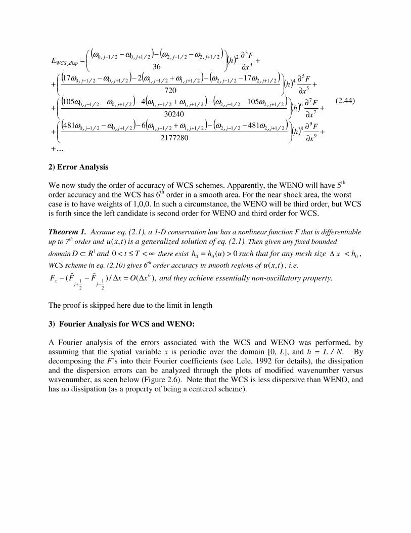
(2.44)

2) Error Analysis

We now study the order of accuracy of WCS schemes. Apparently, the WENO will have 5th

order accuracy and the WCS has 6th

order in a smooth area. For the near shock area, the worst

case is to have weights of 1,0,0. In such a circumstance, the WENO will be third order, but WCS

is forth since the left candidate is second order for WENO and third order for WCS.

Theorem 1. Assume eq. (2.1), a 1-D conservation law has a nonlinear function F that is differentiable

up to 7th order and ),( txu is a generalized solution of eq. (2.1). Then given any fixed bounded

domain1RD ⊂ and ∞<≤< Tt0 there exist 0)(00 >= uhh such that for any mesh size x∆ 0h< ,

WCS scheme in eq. (2.10) gives 6th order accuracy in smooth regions of ),( txu , i.e.

),(/)ˆˆ( 6

2

1

2

1 xOxFFFjj

x ∆=∆−−−+

and they achieve essentially non-oscillatory property.

The proof is skipped here due to the limit in length

3) Fourier Analysis for WCS and WENO:

A Fourier analysis of the errors associated with the WCS and WENO was performed, by

assuming that the spatial variable x is periodic over the domain [0, L], and h = L / N. By

decomposing the F’s into their Fourier coefficients (see Lele, 1992 for details), the dissipation

and the dispersion errors can be analyzed through the plots of modified wavenumber versus

wavenumber, as seen below (Figure 2.6). Note that the WCS is less dispersive than WENO, and

has no dissipation (as a property of being a centered scheme).

Wavenumber

Mo

difie

dW

ave

nu

mb

er

0 0.5 1 1.5 2 2.5 3-1.2

-1

-0.8

-0.6

-0.4

-0.2

0

0.2

Exact

WENOWCS

Dissipation

Wavenumber

Mo

difie

dW

ave

nu

mb

er

0 0.5 1 1.5 2 2.5 30

0.5

1

1.5

2

2.5

3

ExactWENOWCS

Dispersion

(a) Dissipation (b) Dispersion

Figure 2.6 Dissipation and dispersion of WENO and WCS

4) Analysis of weights:

We now proceed to analyze the weight functions for WCS.

Proposition 2 . Assume eq (2.1), a 1-D conservation law has a nonlinear function F that is

differentiable up to 7th order and ),( txu is a generalized solution of eq. (2.1). Then for any given

fixed bounded domain1RD ⊂ and ∞<≤< Tt0 there exist 0)(00 >= uhh such that for any mesh

size 0hx <∆ , WCS or WENO scheme gives a weight function )( 4xOcii ∆+=ω for regions where

),( txu and its derivatives (up to 4th

order) are bounded. Otherwise, )1(Oi =ω .

Again, the proof is skipped here due to the limit in length. All theoretical analyses and proofs

have been documented in our recent three research papers which have been or will be submitted

to scientific journal for review (Su et al, 2007).

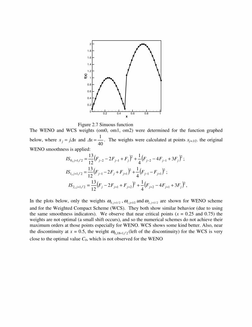
a) Sinuous function

The results in the previous section are only applicable for continuous, smooth functions. Since

the purpose of these numerical schemes is shock-capturing, then an analysis of the properties of

the numerical schemes near a shock is necessary.

In a similar study as in section 2.3, the weights 212211210 and , , /,/,/, +++ jjj ωωω of WENO and

WCS are calculated for the function

( ) ( )( )

≤<−

≤≤=

15021

5002

jj

jjj xx

xxxf

.,sin

.,sin

π

π

(2.45)

plotted below, where xjx j ∆= and 40

1=x∆ .

x

f(x)

0.2 0.4 0.6 0.8 10

0.2

0.4

0.6

0.8

1

1.2

1.4

1.6

1.8

2

Figure 2.7 Sinuous function

The WENO and WCS weights (om0, om1, om2) were determined for the function graphed

below, where xjx j ∆= and 40

1=x∆ . The weights were calculated at points xj+1/2. the original

WENO smoothness is applied:

( ) ( )212

2

12210 344

12

12

13jjjjjjj FFFFFFIS +−++−= −−−−+ /, ;

( ) ( )211

2

112114

12

12

13+−+−+ −++−= jjjjjj FFFFFIS /, ;

( ) ( )212

2

21212 344

12

12

13jjjjjjj FFFFFFIS +−++−= +++++ /, ,

In the plots below, only the weights 2/1,21/2j1,2/1,0 and, +++ jj ωωω are shown for WENO scheme

and for the Weighted Compact Scheme (WCS). They both show similar behavior (due to using

the same smoothness indicators). We observe that near critical points (x = 0.25 and 0.75) the

weights are not optimal (a small shift occurs), and so the numerical schemes do not achieve their

maximum orders at those points especially for WENO. WCS shows some kind better. Also, near

the discontinuity at x = 0.5, the weight 21180 /, +ω (left of the discontinuity) for the WCS is very

close to the optimal value C0, which is not observed for the WENO

x0.2 0.4 0.6 0.8 1

0

0.2

0.4

0.6

0.8

1om0om1om2

WENO WeightsOriginal Smoothness

x0.2 0.4 0.6 0.8 1

0

0.2

0.4

0.6

0.8

1

om0om1om2

WCS WeightsOriginal Smoothness

Figure 2.8 Weights of WENO and WCS for sinuous function

b) Shock tube

-4 -3 -2 -1 0 1 2 3 4 50

0.1

0.2

0.3

0.4

0.5

0.6

0.7

0.8

0.9

1

xj

f(xj)

Figure 2.9 Shock tube function

x-4 -2 0 2 4

0

0.2

0.4

0.6

0.8

1

om0om1om2

WENO WeightsOriginal Smoothness

x-4 -2 0 2 4

0

0.2

0.4

0.6

0.8

1

om0om1om2

WCS WeightsOriginal Smoothness

(a) (b)

Figure 2.10 Weights of WENO and WCS for shock tube

Figure 2.9 and 2.10 show the weights for a shock tube. The weights keep optimal for high

order accuracy, but jump near the shock and expansion wave. We note that the results at the

expansion wave (between -2.5 and 0) are not considered smooth, and the weights are not the

optimal weights. A similar result shows for WCS.

c) Step function

“Step” function

-4 -3 -2 -1 0 1 2 3 4 50

0.1

0.2

0.3

0.4

0.5

0.6

0.7

0.8

0.9

1

xj

f(x j)

Figure 2.11 Step function

-4 -3 -2 -1 0 1 2 3 4 50

0.1

0.2

0.3

0.4

0.5

0.6

0.7

0.8

0.9

1

x

WENO - "step" function - original smoothness

om0om1om2

(a)

-4 -3 -2 -1 0 1 2 3 4 5

0

0.1

0.2

0.3

0.4

0.5

0.6

0.7

0.8

0.9

1

x

WCS - "step" function - original smoothness

om0om1om2

(b)

Figure 2.12 Weights of WENO (a) and WCS (b) for step function

Figure 2.11 and 2.12 show the weights for a step function. In all examples addressed above, the

weights keep optimal for high order accuracy, but jump at four corner points (non-

differentiable). This indicates that we only need to use bias weights at corner points. This

analysis provides a hint that we may waste 95% of computation time. For example, when we use

a thousand grid points but only have 4 corner points, why should we calculate smoothness and

weights for a thousand grid points and solve the tri-diagonal system with variable coefficients at

every time step? This will lead us to develop the version 3 of our black box subroutine with

much high computation efficiency.

2.3.5 Black box subroutine

As addressed in previous sections, after ENO reconstruction, the remained problem is to find a

more accurate derivative for a discrete data set. Based on this understanding, we developed a

black box type subroutine which requires giving an input data set, the data dimension, and finite

difference direction. The subroutine will give back a discrete data as an output derivative. The

idea is that this subroutine can work for any input data no mater it is smooth, oscillatory, or

containing non-differentiable points. Of course, the subroutine should provide high order

accuracy when the data is smooth. A black box type subroutine has been developed, applied in

our own code, and delivered to Air Force Research Lab. This black box can be used anywhere or

any finite difference CFD code. Of course, this is the first version and need to be improved.

2.3.6 Improvement of the algorithm and black box subroutine

We can make improvement to the black box type subroutine at least in several aspects:

1) General Boundary conditions

The current one requires explicit boundary value at each time step which should be given by

the finite difference CFD code. However, we can directly put the boundary conditions to this

black box subroutine by defining:

cxbfxaf bb =+ )(')(

The finite difference scheme will setup high order scheme for this point and the main

program should provide value of a, b, and c. In real world, for a supersonic flow, we have

inflow (Dirichlet, b=0), outflow (Neumann, a=0), far field and solid surface which could be

Dirichlet, Neumenn, or mixed depending on the sign of eigenvalue and heat transfer

condition. The velocity on the wall is always zero and the boundary condition is Dirichlet.

Therefore, the subroutine can self defined with high order for boundary points if the main

program provide the parameters a, b and c for boundary conditions.

2) Optimization of biasF and α

As we apply modification to the flux obtained by WCS, we should optimize the biasF and α

biaswcsmwcs FxFxF ))(1()( αα −+=

The desired biasF should be able to capture strong shock (rapid change in slope) and the

α should control the introduction of biasF and make sure no biasF is introduce off shock and

inside the boundary layer except for necessary high order dissipation. For a discrete data set,

the strong shock will be considered as rapid change corner points and off shock boundary

layer will be thought as smooth data set.

3) Optimization of weights

The WCS is relied on weights to capture the shock and provide necessary dissipation for

damping numerical wiggles. However, the current weights used by our scheme are WENO

weights which shows strong up-winding at corner points and recover to non-bias weights off

the shock quickly. Of course they are good weights, but not the best one. First, the

computation shows the weights did not provide enough dissipation to capture the shock

without wiggles that is why we still need biasF . Second, the weights should provide necessary

high order dissipation even in the smooth area since the WCS is non-dissipative scheme and

cannot damp and existing numerical oscillations. Apparently, we need more work on the

optimization of WCS weights

4) Computation cost reduction

There are concerns which are naturally raised about the computation cost when so many

technologies are used to construct the black box subroutine. However, a large part of cost

will be dramatically reduced when we define a “corner point finder”. The solution is quite

clear. Let us first look for two questions and answers. First one, why do we say WENO

weights are good? The answer is because WENO weights become non-bias and standard

weights to achieve high order. The second question is where the weights changed? The

answer is the weight changes only near the corner points. Therefore, the answer is on our

hand. It does not make much sense that we calculate the smoothness, find the weights,

reconstruct our matrix, and then we did not change anything for most areas except a few

corner points. It turns out we should develop some ways to isolate a few corner points (non-

differentiable) and then modified our coefficients at these points. These will allow us to

dramatically reduce the cost of WCS. In addition, if biasF can be removed, even flux splitting

is not necessary since WCS is central and does not require flux splitting. Really, we spend a

lot of time and computation to calculate smoothness and find WENO weights, but finally we

claim our scheme is very good because our weights are same as standard high order weights

at most points except a few corner points (see above figures). It should be equivalent to make

an adjustment at a few corner points and do nothing for all other points which will be much

cheaper.

5) Self flux splitting

At current time, we still need flux splitting since we use biasF . In future, we plan to develop a

Lax- Friedrich type flux splitting by the black box subroutine itself which will make the

subroutine can treat any data sets no matter what kind governing system is involved.

3. Preliminary Results of the New Schemes

The 3-tep, 3rd

order TVD Runge-Kutta method is applied for time discretization.

3.1 Order of Accuracy

The scheme is tested by solving a linear wave equation with a smooth initial function:

0=+ xt uu , ( ) )2sin(0, xxu π= where 10 ≤≤ x . (3.1)

The calculation stops at 3.0=t and the errors are listed in table 2. The computation shows the

6the order accuracy is achieved.

Table 2. Errors and Order of Accuracy

N L1 Error L1 Order L2 Error L2 Order L∞ Error L∞ Order

8 1.06E02 - 3.67E03 - 2.05E02 -

16 8.66E05 6.93 2.46E05 7.22 2.00E04 6.68

32 1.37E06 5.98 2.94E07 6.39 4.37E06 5.51

64 2.23E08 5.93 3.74E09 6.30 1.11E07 5.30

128 3.45E10 6.01 4.95E11 6.24 2.86E09 5.27

256 4.49E12 6.26 5.73E13 6.43 5.98E11 5.58

3.2. 1-D linear wave equation with jump initial function

The same governing equation is used but the initial condition is discontinuous:

0=+ xt uu , ( ) ≤≤

=otherwise

xifxu

5.0

4.01.00.10, (3.2)

The calculation stops at 3.0=t and the solutions are illustrated in figure 3.1. The results indicate

that standard compact scheme doesn’t work for shocks while both MWCS (UWCNC) presented

in this report and WENO scheme work. Furthermore, MWCS has less dissipation than WENO-5

near shocks which means a sharper transition is obtained.

x

w

0 0.25 0.5 0.75 1

0.5

0.6

0.7

0.8

0.9

1

Standard Compact Scheme

Exact Solution

Figure 3.1 Numerical test over linear wave equation.

3.2 1-D shock tube and shock-entropy interaction

These results have been described in Chapter 2.

3.3 Preliminary results for 2-D shock-boundary layer interaction

In order to test if current MWCS scheme can work for 2-d and 3-D shock – boundary layer

interaction. Three numerical tests are conducted: 1) incident shock; 2) double angles; 3) double

cones. The case with double angles and double cone are still under numerical simulation and

only the case with incident shock is reported here.

A 2-D incident shock-boundary layer interaction (Figure 3.2) was studied by the MWCS. The

Reynolds number is 510 and the Mach number was set to 2.15. The overall pressure ratio is 1.55.

For comparison, the inflow condition was set as same investigated by Degrez et al (1987). Their

experimental work has shown the shock-boundary layer interaction is laminar and two-

dimensional. Therefore, we can do a 2-D numerical simulation and compare with their

computational and experimental results. The computational grids is 257x257 (Figure 3.3). The

grid stretching in stremwise direction is 1.01. The stretching in normal direction is 1.015. A 2-D

Navier-Stokes equation is solved as the governing equation.

x

f

0 0.25 0.5 0.75 1

0.5

0.6

0.7

0.8

0.9

1

UWCNC

WENO-5

Exact Solution

Figure 3.2 Sketch of incident shock-boundary Figure 3.3 Computation Grids (257x257)

layer interaction

Figure 3.4 Pressure distribution: left is a normal view and right is stretched in the normal

direction by a factor of 5

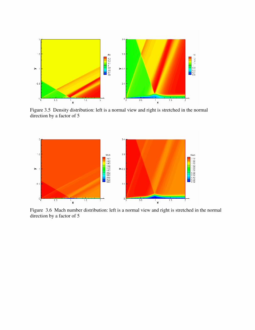
Figure 3.5 Density distribution: left is a normal view and right is stretched in the normal

direction by a factor of 5

Figure 3.6 Mach number distribution: left is a normal view and right is stretched in the normal

direction by a factor of 5

Figure 3.7 Temperature distribution: left is a normal view and right is stretched in the normal

direction by a factor of 5

Figure 3.8 Comparison of pressure distribution on the wall surface. (The red one is our

computation, the black dash one and solid one are Degrez’s computation and experiment

respectively)

Figure 3.9 Comparison of velocity profiles at different locations (The red one is our computation,

the black solid line and black square are Degrez’s computation and experiment respectively)

Figures 3.4-3.7 show the distribution of pressure, density, Mach number and temperature

obtained by our computation. Figure 3.8 and 3.9 show our numerical results agree well with the

numerical results and are close to the experimental results given by Degrez et al (1987). Degrez

et al favor their computational results addressed in their JFM paper. Figure 3.10 shows MWCS

scheme has higher resolution for 2-D incident shock-boundary layer interaction. These results

show our scheme can be extended to 2-D and 3-D problems.

Figure 3.10 Verticity of 2-D incident shock-boundary layer interaction: (a) WENO (b) MWCS

3.4 Preliminary results for 2-D double angle shock-boundary layer interaction at M=9.59

In order to validate our scheme and code, we should compare our results with well documented

experimental and computational data. The case including the geometry and inflow condition was

set same as the experiment conducted by Wadhams et al (2004) and the computation by

Gaitonde et al (2002). The inflow Mach number is set to M=9.58, the Reynolds number

Re=278870, the inflow temperature Tin=185.6, and the wall temperature Tw=293.3.

Before we work on a double cone, we solve a supersonic flow passing a double angle first. The

overall Grid is 257x129 obtained by elliptic grid generation and the girds are uniform in stream-

wise direction, but stretched in wall normal direction with a factor of 1.037. The grids, contour of

flow filed and distribution of physical quantities along the wall boundary are shown in Figure

3.11-3.13. Since the case we calculated is for a double angle not a double cone, we cannot

compare with the above experiment and computation directly for now. However, the distribution

of mach number, pressure, density, and temperature are very similar. Further development will

be set for double cones at M=9.59 which will allow us to compare our computational results with

the above experiment and computation.

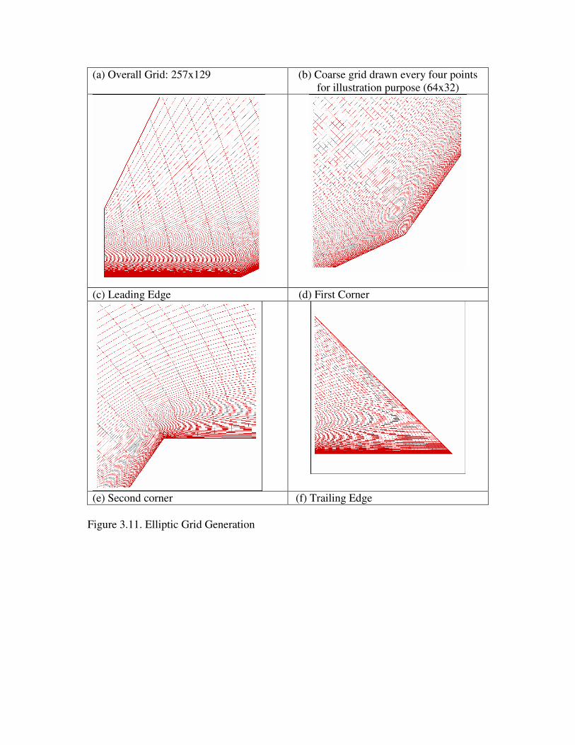
(a) Overall Grid: 257x129 (b) Coarse grid drawn every four points

for illustration purpose (64x32)

(c) Leading Edge (d) First Corner

(e) Second corner (f) Trailing Edge

Figure 3.11. Elliptic Grid Generation

Figure 3.12. Contours of flow field (Mach number, pressure, density, temperature, stream line,

and separation bubble)

Figure 3.13 Distribution of physical quantities (pressure, density, and temperature) along the

wall boundary:

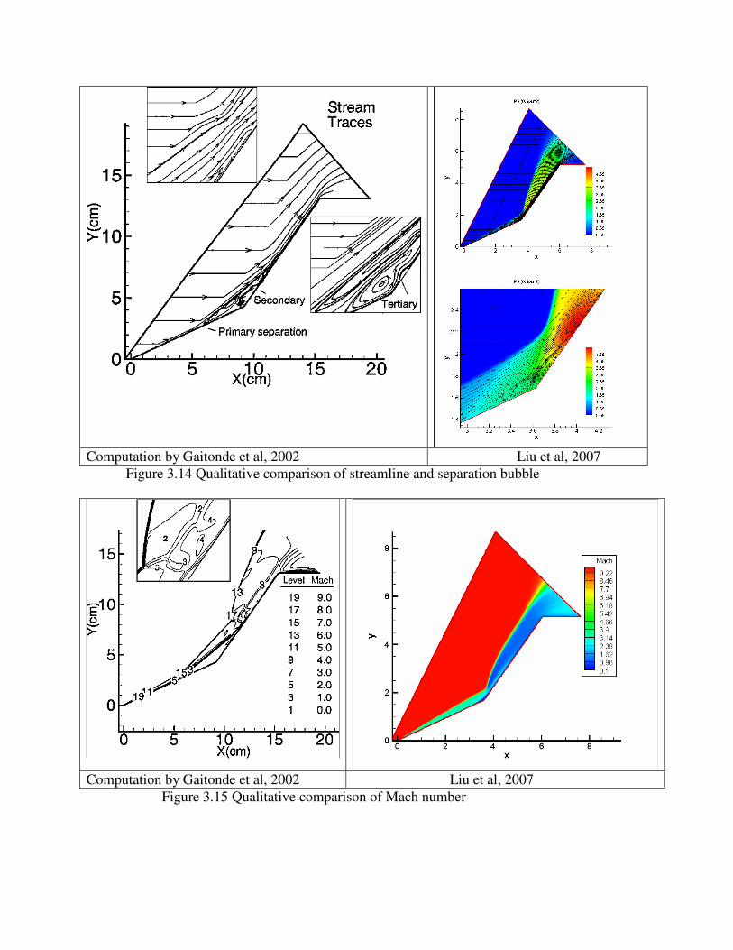
Although we used same geometry and inflow conditions as the experiment (Wadhams et al,

2004) and the computation used, we cannot directly compare our results with theirs since their

results are for double cones and ours for double angles. However, we can make qualitatively

comparison and find the flow structure is very similar. Figure 3.14-3.17 show such a comparison.

x

T

0 2 4 6 8-500

0

500

1000

1500

2000

2500

x

rho

0 2 4 6 8-5

0

5

10

15

20

25

30

x

p

0 2 4 6 8-50

0

50

100

150

200

250

300

Computation by Gaitonde et al, 2002 Liu et al, 2007

Figure 3.14 Qualitative comparison of streamline and separation bubble

Computation by Gaitonde et al, 2002 Liu et al, 2007

Figure 3.15 Qualitative comparison of Mach number

Experiment (Wadhams et al, 2004)

and Computation (Gaitonde et al, 2002)

Liu et al, 2007

Figure 3.16 Qualitative comparison of Cp

Experiment (Wadhams et al, 2004) Liu et al, 2007

Figure 3.17 Qualitative comparison of pressure distribution

3.5 Preliminary results for 2-D double cone shock-boundary layer interaction at M=9.58

This work is still under development.

3. 6 Achievements and further efforts

The following conclusions can be made based on our previous work which was supported by the

current AFOSR grant ending by 12-31-07:

1) The original weighted compact scheme does not have enough dissipation to capture the

shock without wiggles but is too dissipative in the smooth region.

x0 2 4 6 8

-1

0

1

2

3

4

5

P / (0.5 u^2)ρ

x0 2 4 6 8

-1

0

1

2

3

4

5

6

(P - P_inf) / (0.5 u 2)ρ

2) The second order smart filter can help the WCS scheme remove the wiggles near the

shock. However, the filter is case related and needs professional training to adjust.

3) The new MWCS scheme is basically a WCS scheme modified by a high order bias

scheme. MWCS is in general much better in capturing both shock and small length scales

than the standard 5th

order WENO scheme and potentially could become an very

important tool for DNS and LES of the shock and turbulent boundary layer interaction.

4) MWCS has sixth order of accuracy in the smooth area. For near shock grid points,

weights 0,0,1 210 === ωωω , MWCS still has fourth order of accuracy. Comparing

with 5th

order WENO which has 5th

order in the smooth area and third order near the

shock, MWCS is super with smaller stencils and higher order of accuracy.

5) MWCS is applicable for the simulation of flows containing both shock waves and small

structures. This scheme uses same formulation without switching to a different scheme or

using a low order filter.

During the past three years, following achievements have been made:

1) Developed a modified weighted compact scheme

2) Applied the MWCS scheme for 1-D shock tube and 1-D shock-entropy interaction and

obtained very promising results

3) Applied the MWCS for 2-D incident shock, double angle and double cones. The incident

shock results are very encouraging and the computation for double angle looks very

reasonable while the double cone case is still under development.

4) Conducted theoretical study on the analysis of accuracy, dissipation, dispersion and

weights function for both MWCS and WENO.

5) Developed a universal, black-box subroutine, applied it in our finite difference scheme,

and delivered it to the Air Force research Lab. The subroutine can accept any discrete

data as input and give a high order derivative as output, which can be used by any finite

difference computation codes.

Future work will include more 2-D and 3-D shock-boundary layer interaction cases,

optimization of WCS weights, modifying biasF and )(xα , improve the black box subroutine

and dramatically reduce the computational cost required by the subroutine. In addition, we

will also focus our effort on mathematical investigation of our new approaches including the

accuracy, stability, dissipation, dispersion, modified governing equations, etc. The

mathematical foundation is critical for new scheme development. If we do not understand

well, it would not be possible to improve or optimize the new scheme.

4. Acknowledgement

This work is supported by AFOSR under grant FA9550-05-1-0136 supervised by Dr.

Fahroo. The author thanks Dr. Fahroo for her sponsorship. The author also thanks Dr.

Gaitonde for his support through VA Summer Faculty Program.

4. References

[1] Gaitonde, D, and Visbal, M, Pade-type high-order boundary filters for the Navier-Stokes

equations, AIAA Journal, Vol. 38, No. 11, pp 2103-2112, 2000.

[2] Gaitonde, D, Canupp, p. W., and Holden, M., Heat transfer predictions in a laminar

hypersonic viscous/inviscid interaction, Journal of thermophysics and heat transfer, Vol. 16, No.

4, October–December 2002

[3] Godnov, S. K., A difference scheme for numerical computation of discontinuous solution of

hydrodynamic equations, Math Sbornik, Vol 47, 271-306 (in Russian) translated US Joint Publ.

Res. Service, JPRS 7226, 1969.

[4] Harten A, High resolution schemes for hyperbolic conservation laws, J. of Computational

Physics, Vol 49, pp357-393, 1983.

[5] Harten A, Engquist B, Osher, B, Charkravarthy SR, Uniformly high order accurate

essentially non-oscillatory schemes III, J. of Computational Physics, Vol 71, pp231-303,

1987.

[6] Jiang, G. S., Shu, C. W., Efficient implementation of weighted ENO scheme. J. Comput.

Phys., 126, pp.202—228, 1996.

[7] Jiang L, Shan H, Liu C, Weight Compact Scheme for Shock Capturing, International Journal

of Computational Fluid Dynamics, 15, pp.147-155, 2001.

[8] Lele S.K., Compact finite difference schemes with spectral-like resolution, Journal

Computational Physics, 103, pp.16—42, 1992.

[9] Liu, C., Xie, P., and Olveira, M, High order modified compact scheme for high speed flow,

technical report to Gaitonde at Air Force Research Lab.

[10] Liu, D, Osher, S, Chan, T, Weighted essentially nonoscilltory schemes, J. of Computational

Physics, V115, pp200-212, 1994

[11] Roe, P.L., Approximate Riemann solvers, parameter vectors and difference schemes, J. of

Computational Physics, Vol 43, pp357-372, 1981

[12] Shu, C.W., Osher, S., Efficient implementation of essentially non-oscillatory shock-

capturing scheme. Journal of Computational Physics 77, pp.439-471, 1988.

[13] Shu, C. W., Osher, S., Efficient implementation of essentially non-oscillatory shock-

capturing schemes II, J. Comput. Phys.,83, pp.32-78, 1989.

[14] Su, Xie, Oliveira, and Liu, Error Analysis for Weighted Higher Order Compact Finite

Difference Scheme, J. of Applied Mathematical Science, to appear.

[15] Van Leer, B., Towards the ultimate conservative difference scheme. V. A second order

sequel to Godnov’s scheme, Journal of Computational Physics, Vol 32, pp101-136, 1979

[16] Visbal, M. and Gaitonde, D., On the use of higher-order finite-difference schemes on

curvilinear and deforming mashes’ JCP, Vol. 181, pp155-158, 2002.

[17] Wadhams, T. P., Holden, M. S., Summary of experimental studies for code validation in

the LENS facility with recent Navier-Stokes and DSMC solutions for two- and three-

dimensional separated regions in hypervelocity flows, AIAA 2004-917 42nd AIAA Aerospace

Sciences Meeting and Exhibit, 5 - 8 January 2004, Reno, Nevada