High Performance Computing - Introduction to Parallel

Programming II

Prof Matt Probert http://www-users.york.ac.uk/~mijp1

Overview

•  Types of Problem Decomposition – Trivial decomposition – Functional decomposition – Data decomposition

•  Performance Analysis

Parallel Problem Decomposition •  Discussed basics of parallelism at the code

level, machine architectures, etc previously. •  Now focus on how to think in parallel

– Need to consider devising parallel algorithms and strategies, e.g. problem decomposition

•  Three basic approaches: – Trivial parallelism – Functional decomposition – Data decomposition

Trivial Parallelism •  For some problems, need to do systematic scan

of parameter space, or repeat several times to get an average, etc.

•  Hence do not need to parallelise code at all! –  Run separate instances of serial code on different

CPUs, each having different set of input parameters –  No communication between CPUs (except by user at

end to gather final results) –  Perfect scaling, no need to rewrite code, no

problems with load balancing, etc. Trivial but still useful

•  BUT not very flexible – presumes each simulation is independent of all others and does not allow bigger problems to be tackled – each instance has to fit onto a single CPU.

Functional Decomposition •  Divide overall task into separate sub-tasks and

assign each sub-task to different CPUs –  E.g image processing:

–  As each CPU finishes its task it passes data to next CPU and receives data from previous CPU

–  A.k.a. pipelining – as used in CPU/GPU –  Very problem dependent – amount of parallelism

depends on nature of task not size of dataset

Functional Decomposition Drawbacks •  Startup cost

–  As with any pipeline, there is a startup cost. The 2nd CPU cannot do anything until 1st has finished its first task. Ditto 3rd, 4th, etc.

–  Similarly at end when shutdown process •  Load balancing

–  Need to take care to ensure each sub-task completes in approx. same amount of time otherwise one slow sub-task will cause all “downstream” sub-tasks to stall.

•  Scalability –  Once task has been divided up into N sub-tasks then

will only benefit from a maximum of N CPUs –  Also limit to maximum size of problem that can handle

Data Decomposition •  The most flexible approach to parallelism •  Data divided up between CPUs

– Each CPU has its own chunk of the dataset to operate upon and then results collated

– Need to ensure load balancing •  Implies equal size tasks not equal size datasets •  Can do static load balancing, e.g. if geometry of

datagrid is not changing and can partition effectively

•  Can do dynamic load balancing if assign all large tasks first, and then back-fill with smaller tasks until all tasks completed

•  Common approaches include task farming and regular grid decompositions …

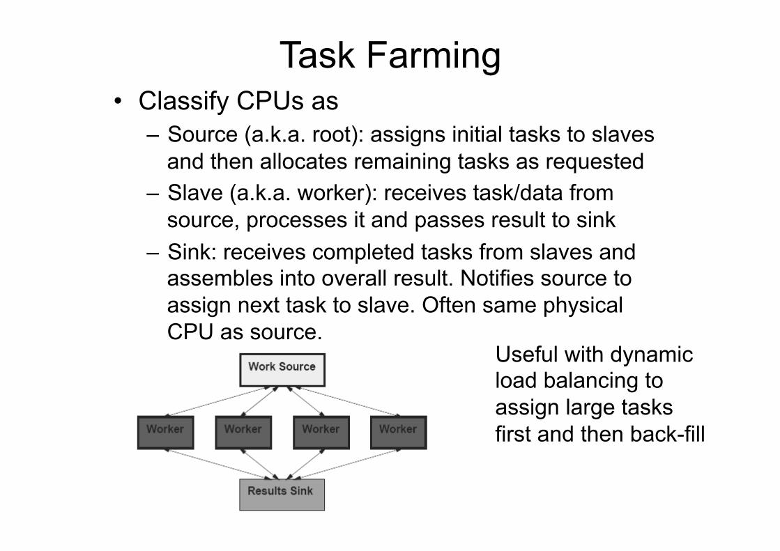
Task Farming •  Classify CPUs as

–  Source (a.k.a. root): assigns initial tasks to slaves and then allocates remaining tasks as requested

–  Slave (a.k.a. worker): receives task/data from source, processes it and passes result to sink

–  Sink: receives completed tasks from slaves and assembles into overall result. Notifies source to assign next task to slave. Often same physical CPU as source.

Useful with dynamic load balancing to assign large tasks first and then back-fill

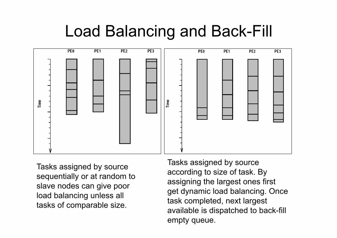
Load Balancing and Back-Fill

Tasks assigned by source sequentially or at random to slave nodes can give poor load balancing unless all tasks of comparable size.

Tasks assigned by source according to size of task. By assigning the largest ones first get dynamic load balancing. Once task completed, next largest available is dispatched to back-fill empty queue.

Task Farm Drawbacks •  One of the oldest models of parallelism

–  Easiest with independent tasks as then similar to functional decomposition

•  Slaves may be idle whilst waiting assignment of next task –  Can overcome this if each slave has a task buffer to

store next task before it is needed •  Can involve a large amount of communications

for a limited amount of calculation (if tasks are small) –  And difficult to handle comms if do not know in

advance which slave will be working on which chunk •  Hence grid decomposition is more common …

Grid Decomposition

•  Many HPC problems involve operating on a very large dataset, arrays, etc. – By dividing data into smaller grids can then

assign each to a separate set of processes – May need special treatment to handle “edges”

of grids where different processes overlap – Enables very large problems to be tackled as

no single process has to contain everything – Very flexible and powerful approach

Regular Grid Decomposition

•  Global data grid is divided into regular sub-grids

•  Each sub-grid is then assigned to different processes as its local data block

•  Best if can match network topology to decomposition

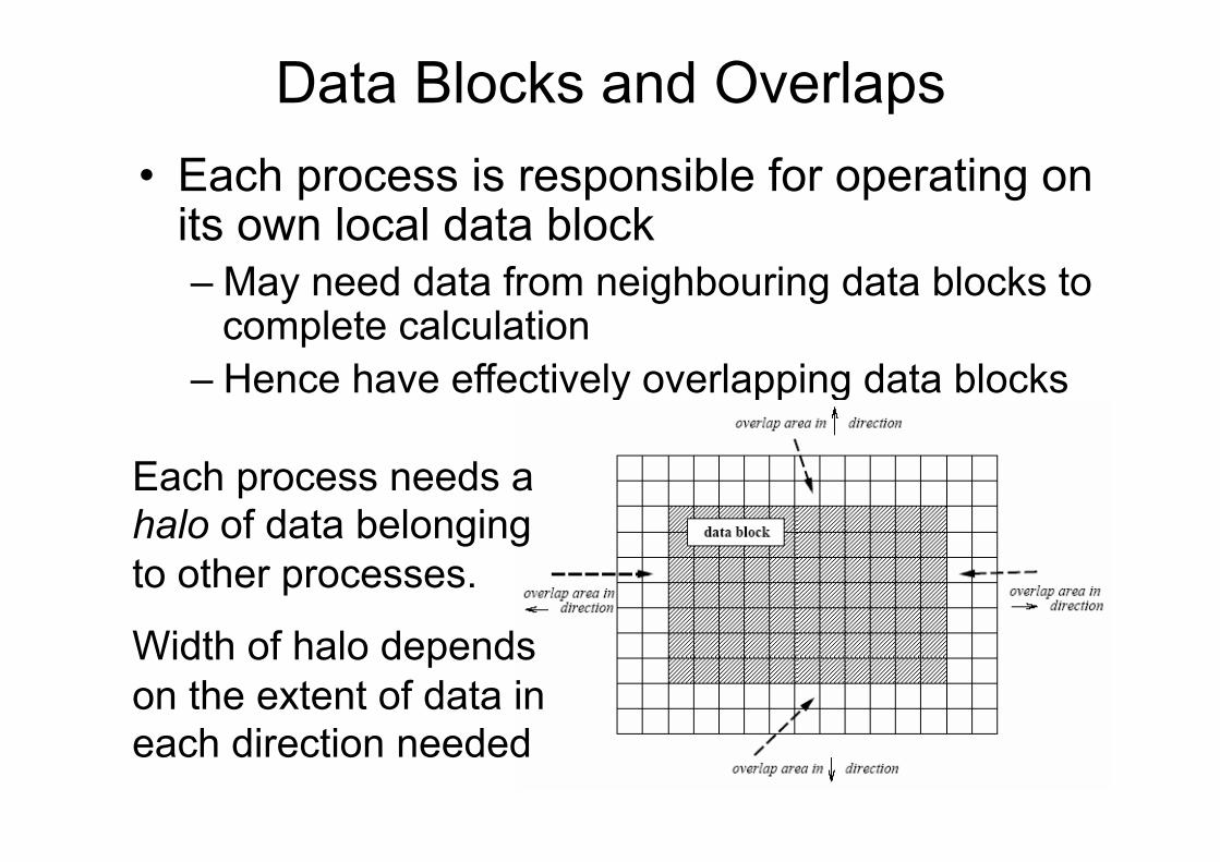
Data Blocks and Overlaps •  Each process is responsible for operating on

its own local data block – May need data from neighbouring data blocks to

complete calculation – Hence have effectively overlapping data blocks

Each process needs a halo of data belonging to other processes.

Width of halo depends on the extent of data in each direction needed

Halos and Updates •  To complete an update, each process may

have to interchange data with its neighbours in order to keep all halos up-to-date.

•  This is known as halo- or boundary-swapping

Thickness of overlap region depends on granularity of decomposition.

As the number of processes increases, the granularity becomes finer and so the overlap increases which limits gains of parallelism.

Boundary Swapping •  If the only data elements modified are purely

internal to a data block, then there is no need to update neighbouring blocks.

•  Otherwise, must: 1.  Send off copies of any data elements to neighbours

that they might require, e.g. halo data 2.  Receive copies of data from neighbours and put into

appropriate locations in data block 3.  Update every element of local data 4.  And then repeat 1-3 for next iteration •  But what about the outside edge of the global

data grid? Need some boundary conditions!

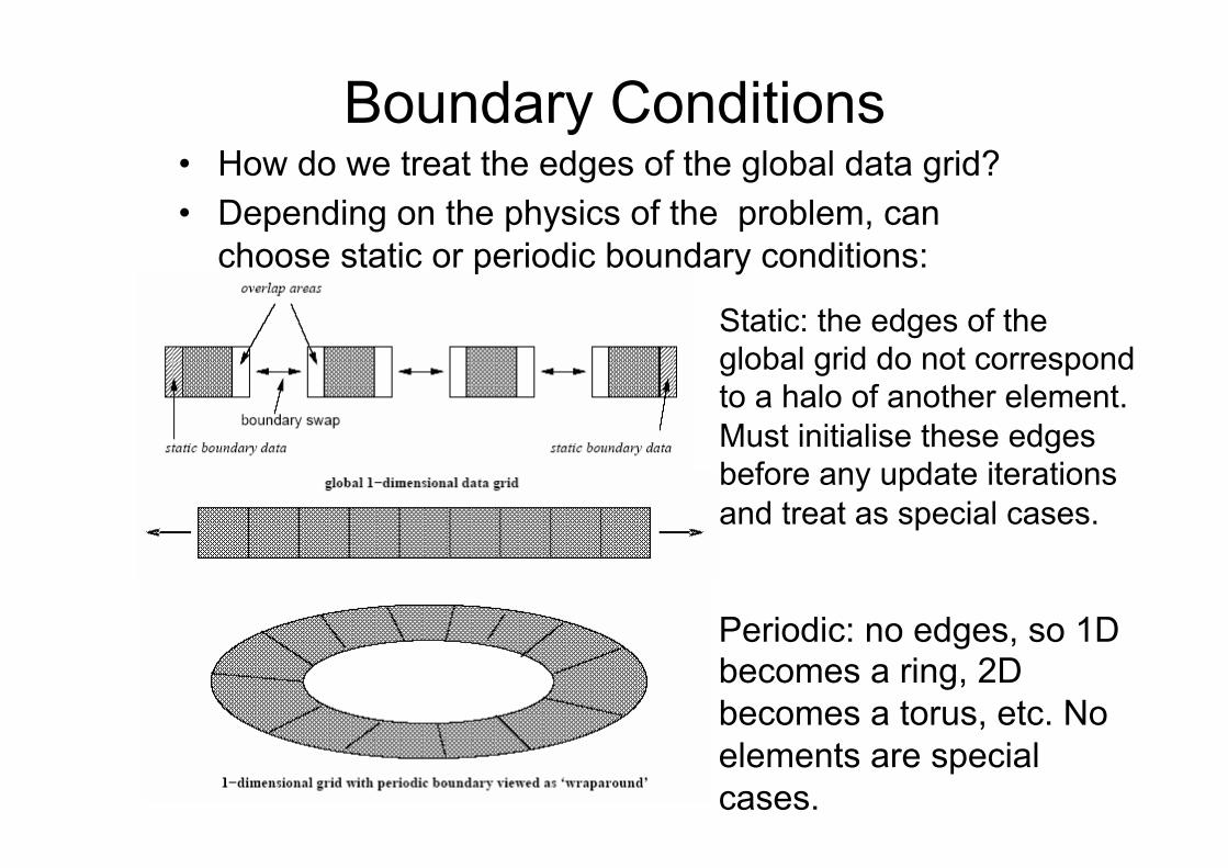
Boundary Conditions •  How do we treat the edges of the global data grid? •  Depending on the physics of the problem, can

choose static or periodic boundary conditions:

Static: the edges of the global grid do not correspond to a halo of another element. Must initialise these edges before any update iterations and treat as special cases.

Periodic: no edges, so 1D becomes a ring, 2D becomes a torus, etc. No elements are special cases.

Unbalanced Grids •  If the problem naturally maps onto a

regular data grid, and the amount of work required is similar per process then all is well.

•  But what if the amount of work per processor varies? – Execution time will then be dominated by

process with most work – Spoils load balancing and hence is inefficient – Hence better to ensure work is evenly

distributed rather than data

Ocean Modelling I •  Classic case study – divide spherical surface

into 3D-grid of latitude, longitude and depth •  Even distribution of data would be inefficient

as differing amounts of land (no work) and depths of ocean (lots of work)

But we know in advance where the land and deep ocean parts are, and they do not change during simulation.

Hence can adjust decomposition until similar amount of work per process.

Ocean Modelling II •  Irregular data distribution:

–  0 represents land, other numbers show which CPU holds the data

Example is for CPU #4: central area is local to #4 and is not involved in any comms; inner halo shows data owned by #4 and shared with others; outer halo shows data owned by others

Performance Issues •  Clearly the irregular data distribution involves

more comms than the regular version –  Hence only worthwhile if saving in calculation

offsets the comms costs •  More difficult if distribution is not known in

advance or changes with time •  Might try a cyclic distribution to even out load

imbalance –  E.g. divide data geometrically into many more

areas than CPUs, so likely that each CPU gets similar amounts of work. But this destroys spatial locality of data and can be inefficient. Hence need to be careful!

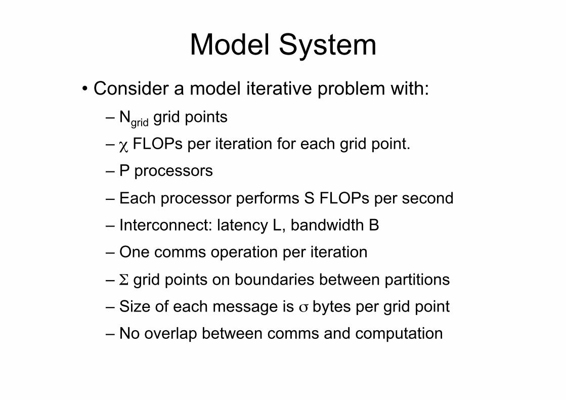
Model System •  Consider a model iterative problem with:

–  Ngrid grid points

–  χ FLOPs per iteration for each grid point.

–  P processors

–  Each processor performs S FLOPs per second

–  Interconnect: latency L, bandwidth B

–  One comms operation per iteration

–  Σ grid points on boundaries between partitions

–  Size of each message is σ bytes per grid point

–  No overlap between comms and computation

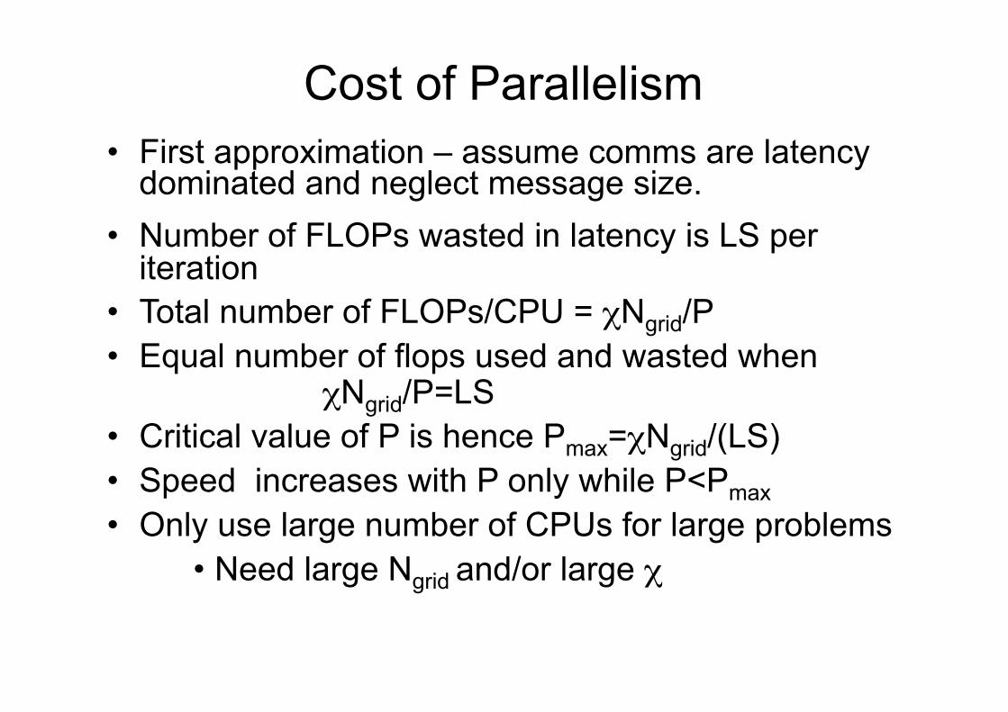
Cost of Parallelism •  First approximation – assume comms are latency

dominated and neglect message size. •  Number of FLOPs wasted in latency is LS per

iteration •  Total number of FLOPs/CPU = χNgrid/P •  Equal number of flops used and wasted when

χNgrid/P=LS •  Critical value of P is hence Pmax=χNgrid/(LS) •  Speed increases with P only while P<Pmax •  Only use large number of CPUs for large problems

• Need large Ngrid and/or large χ

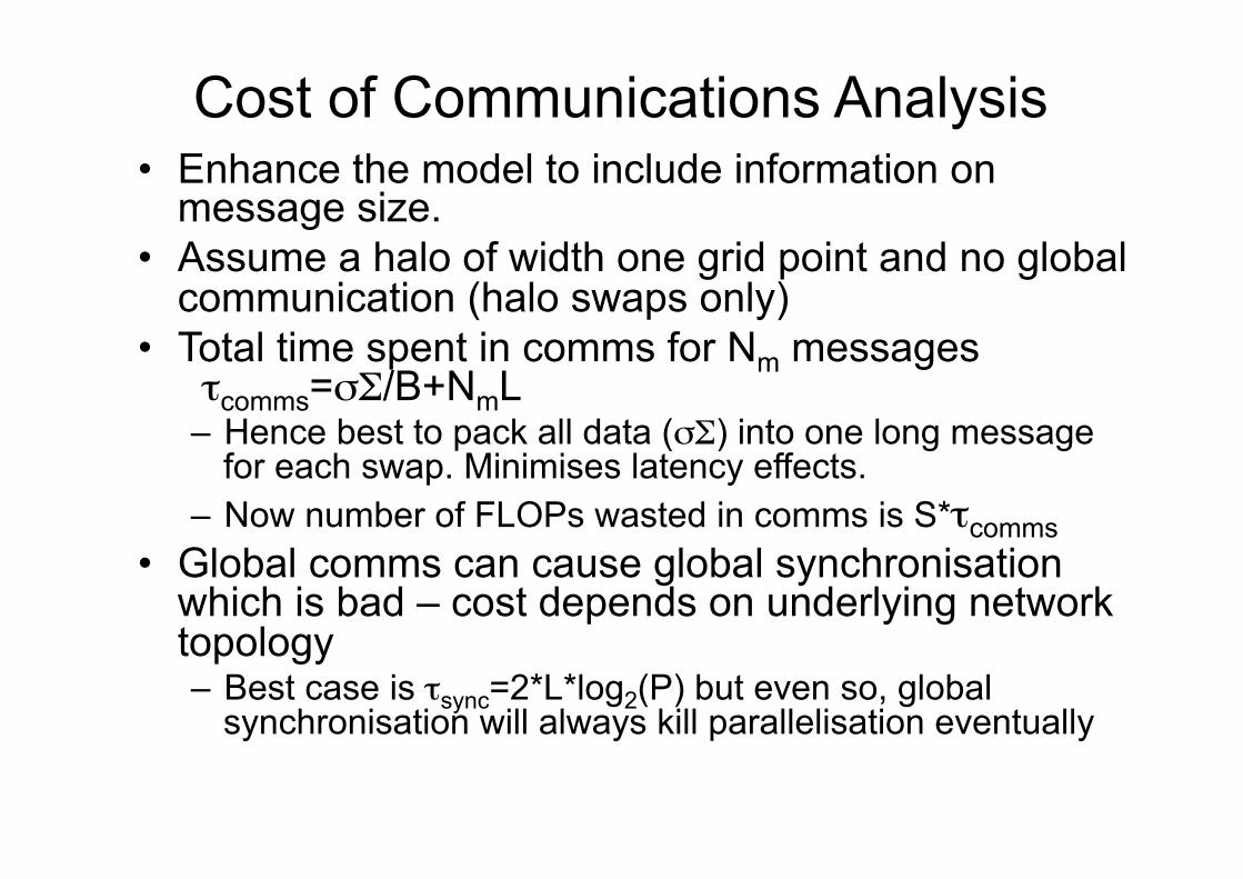
Cost of Communications Analysis •  Enhance the model to include information on

message size. •  Assume a halo of width one grid point and no global

communication (halo swaps only) •  Total time spent in comms for Nm messages

τcomms=σΣ/B+NmL –  Hence best to pack all data (σΣ) into one long message

for each swap. Minimises latency effects. –  Now number of FLOPs wasted in comms is S*τcomms

•  Global comms can cause global synchronisation which is bad – cost depends on underlying network topology –  Best case is τsync=2*L*log2(P) but even so, global

synchronisation will always kill parallelisation eventually

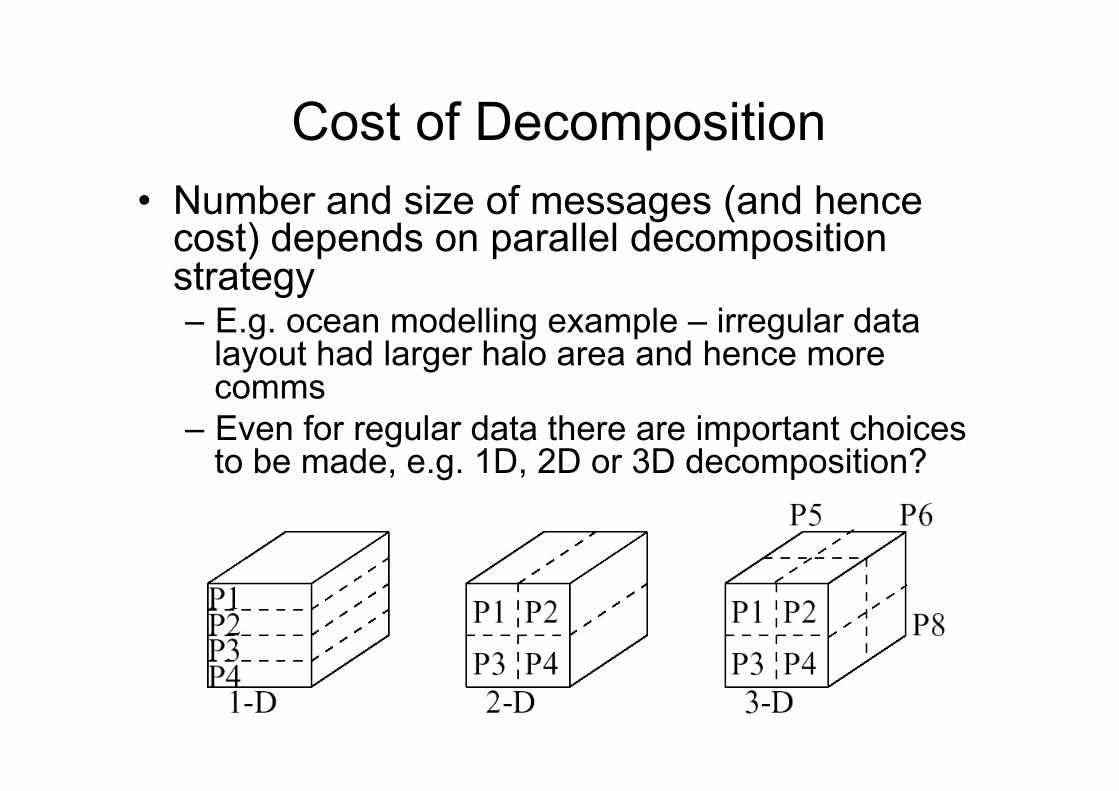
Cost of Decomposition •  Number and size of messages (and hence

cost) depends on parallel decomposition strategy – E.g. ocean modelling example – irregular data

layout had larger halo area and hence more comms

– Even for regular data there are important choices to be made, e.g. 1D, 2D or 3D decomposition?

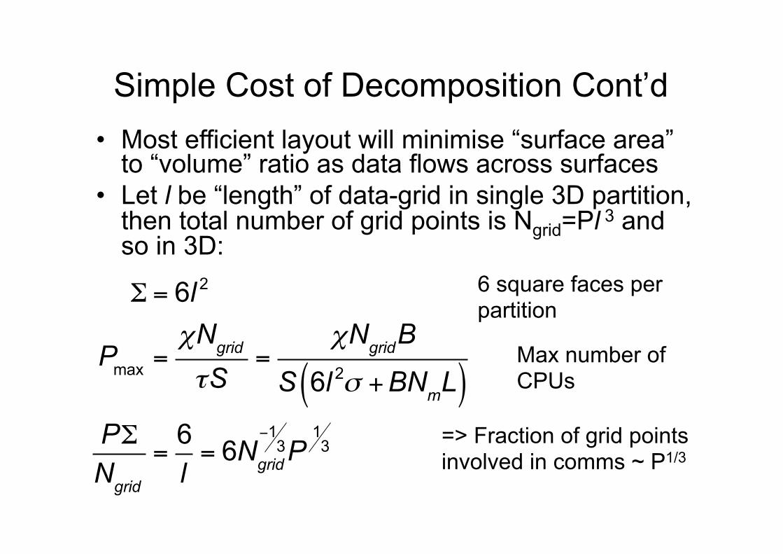
Simple Cost of Decomposition Cont’d •  Most efficient layout will minimise “surface area”

to “volume” ratio as data flows across surfaces •  Let l be “length” of data-grid in single 3D partition,

then total number of grid points is Ngrid=Pl 3 and so in 3D:

=> Fraction of grid points involved in comms ~ P1/3

6 square faces per partition

Max number of CPUs

Σ = 6l 2

Pmax =χNgrid

τS=

χNgridB

S 6l 2σ +BNmL( )PΣNgrid

=6l= 6Ngrid

−13P

13

Simple Cost of Decomposition Cont’d •  2D:

4 rectangular faces involved in comms

=> Fraction of grid points involved in comms ~ P1/2

Ngrid = Pl2Ngrid

13

Σ = 4lNgrid

13

Pmax =χNgridB

S 4lNgrid

13σ +BNmL

"

#$

%

&'

PΣNgrid

=4l= 4Ngrid

−13P

12

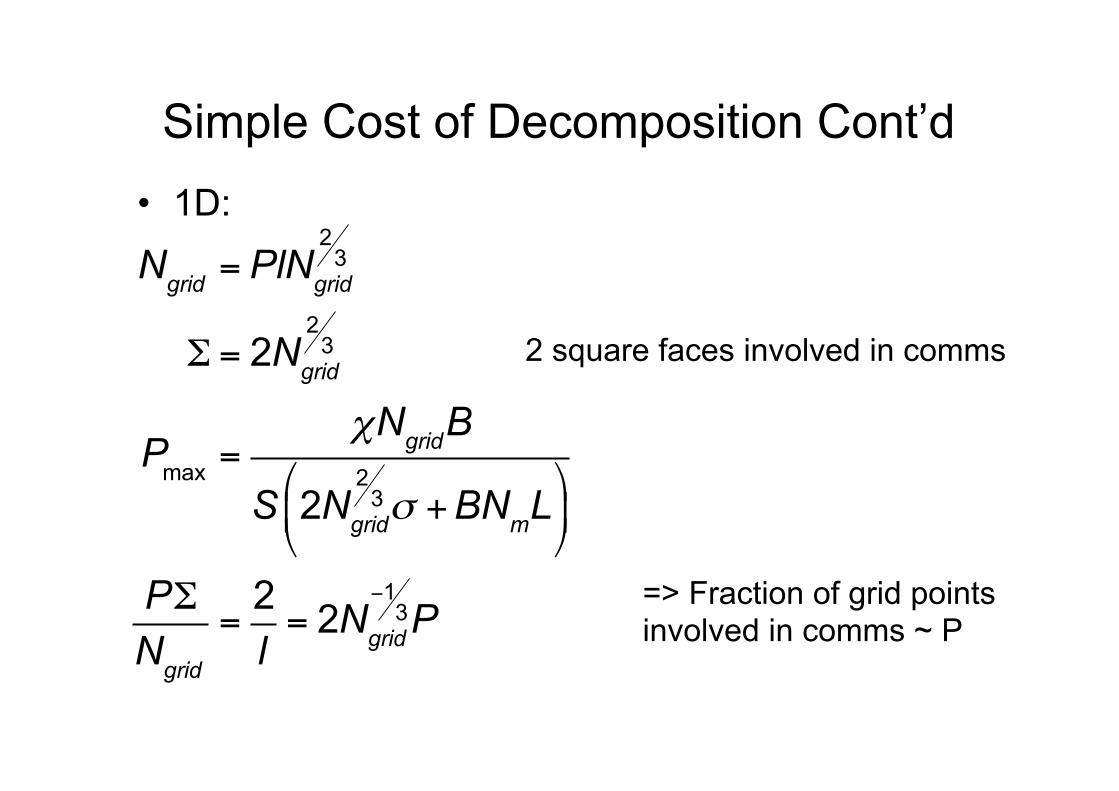
Simple Cost of Decomposition Cont’d •  1D:

2 square faces involved in comms

=> Fraction of grid points involved in comms ~ P

Ngrid = PlNgrid

23

Σ = 2Ngrid

23

Pmax =χNgridB

S 2Ngrid

23σ +BNmL

"

#$

%

&'

PΣNgrid

=2l= 2Ngrid

−13P

Performance

•  1D wins for small P, 3D wins for large P. •  NB this analysis is for 1D, 2D or 3D decomposition of 3D

problem. Need to redo analysis for a 1D or 2D problem!

Further Reading •  Chapter 5 of “Introduction to High

Performance Computing for Scientists and Engineers”, Georg Hager and Gerhard Wellein, CRC Press (2011).

•  Edinburgh Parallel Computer Centre tutorials at http://www.epcc.ac.uk