High Performance FFT Based Poisson Solver on a CPU-GPU HeterogeneousPlatform

Jing WuDepartment of Electrical and Computer Engineering

and Institute for Advanced Computer StudiesUniversity of Maryland

College Park, MDEmail: jingwu@umiacs.umd.edu

Joseph JaJaDepartment of Electrical and Computer Engineering

and Institute for Advanced Computer StudiesUniversity of Maryland

College Park, MDEmail: joseph@umiacs.umd.edu

Abstract—We develop an optimized FFT based Poissonsolver on a CPU-GPU heterogeneous platform for the casewhen the input is too large to fit on the GPU global memory.The solver involves memory bound computations such as 3DFFT in which the large 3D data may have to be transferredover the PCIe bus several times during the computation.We develop a new strategy to decompose and allocate thecomputation between the GPU and the CPU such that the3D data is transferred only once to the device memory, andthe executions of the GPU kernels are almost completelyoverlapped with the PCI data transfer. We were able to achievesignificantly better performance than what has been reportedin previous related work, including over 50 GFLOPS for thethree periodic boundary conditions, and over 40 GFLOPS forthe two periodic, one Neumann boundary conditions. The PCIebus bandwidth achieved is over 5GB/s, which is close to thebest possible on our platform. For all the cases tested, thesingle 3D PCIe transfer time, which constitutes a lower boundon what is possible on our platform, takes almost 70% of thetotal execution time of the Poisson solver.

Keywords-Fast Fourier Transforms; Parallel and Vector Im-plementations; GPU; CUDA; Poisson Equations

I. INTRODUCTION

There has been recent interest in the development ofhigh performance direct Poisson solvers due partly to theintroduction of immersed-boundary methods [12]. Poissonsolvers are an extremely important tool used in many appli-cations, which most often constitute the most computation-ally demanding component of the application. In an earlierwork [18], we developed an FFT-based direct Poisson solverfor GPUs, which was optimized for the case when the 3Dgrid fits onto the device memory. The performance reportedthere assumes that both the input and output reside on thedevice memory, which is the typical assumption made bymost of the published GPU algorithms. In this work, weconsider the case when the grid is much larger than thesize of the device memory, but can still fit in the mainmemory of a multicore CPU, and develop an optimizedFFT-based direct Poisson solver on such a platform. Ourapproach exploits the particular strengths of each processorwhile carefully managing the data transfers needed between

the CPU and the GPU. In particular, our algorithm includesoptimized 2D or 3D FFT implementations and optimizedtridiagonal solver implementations for such a heterogeneousenvironment in which both the input and the output residein the main memory of the CPU.

Most of the recently published work of FFT algorithmson GPUs [8][10][14][13][9][3], assume data sizes limited bythe device memory size. This assumption results in effortsthat are concentrated on GPU optimization, including datatransfers between device memory and the shared memoryor registers of the streaming multiprocessors. For memorybound computations, such as FFTs, the performance bottle-neck becomes the device memory bandwidth and the typeof the global memory accesses. For recent GPUs, the peakdevice memory bandwidth is higher than 100 GB/s.

We compare our results to two recent results on a similarmodel. Chen et al [1] used a cluster of 4 or 16 nodes,each node includes two GPUs (Tesla C1060 and GTX 285),to handle large 3D FFT computations. They reported aperformance of around 50 GFLOPS on four nodes, some-what lower than our performance on a single node with aTesla C1060 (in fact, our performance number is an under-estimate since it does not include all the components ofour Poisson solver). Another recent work is reported byGu et al [11], which tries to optimize both CPU-GPU datatransfer and GPU computations for 1D, 2D, and 3D FFTs.In particular, they develop a blocked buffered technique for1D FFTs which achieves a high bandwidth on the CPU-GPU data channel. For their multidimensional FFTs, the datahas to be transferred back and forth between the CPU andGPU at least twice, and for 3D double-precision FFT, theirbest performance is around 15 GFLOPS on the NVIDIATesla C2070, 13 GFLOPS on the NVIDIA GTX480 and9 GFLOPS on the NVIDIA Tesla C1060 respectively. Ourperformance numbers for the single-precision FFTs reach 60GFLOPS using the Tesla C1060.

We develop a new approach that introduces the followingcontributions:

• The computation is organized in such a way that the

3D grid data is transferred between the CPU memoryand the device memory only once, while achieving aPCIe bus bandwidth close to the best possible on ourplatform.

• The GPU kernel computations are almost completelyoverlapped with the data transfers on the PCIe bus, andhence the GPU execution time contributes very little tothe overall execution time. This is due to an effectiveuse of the CUDA page-locked host memory allocation,asynchronous function calls, and write-combining.

• Our approach makes effective use of the multithreadedarchitectures of both the CPU and GPU. In particular,the FFTs along the X-dimension are partially computedon the multicore CPU in a way that exploits thepresence of the processor cores and the L3 cache, andthe rest of the computations are carried out on theGPU using a minimum number of coalesced memoryaccesses with all operations executed directly on theregisters.

• While our implementation achieves an accuracy com-parable to a double precision implementation, our FFTbased direct Poisson solver uses primarily single preci-sion floating operations, which effectively doubles theeffective bandwidth of data movement for the same datasizes.

• Experimental tests on our platform for problems oflarge sizes show that almost 70% of the total executiontime is consumed by the single 3D grid data transferover the PCIe bus, and most of the rest is consumed bythe initial CPU computation of the partial FFT alongthe X dimension. The overall performance of our FFT-based Poisson solver ranges between 50 GFLOPS and60 GFLOPS.

II. OVERVIEW AND BACKGROUND

In this section, we provide an overview of the algorithmsbehind the FFT-based Poisson solver, which include FFTand tridiagonal linear system computations. Basic FFT al-gorithms that are related to our work are then summarized,followed by an overview of Thomas’ algorithm for solvingtridiagonal linear systems. We end this section with anoverview of the general architecture of our platform thatconsists of a multicore processor with a GPU accelerator.

A. FFT-based Poisson SolverThe three-dimensional Poisson equation is defined by:

∇2φ =∂2φ

∂x2+∂2φ

∂y2+∂2φ

∂z2= f, in Ω, (1)

In our earlier work [17], we presented algorithms forthe FFT-based Poisson solver, which were optimized forgrid sizes that fit in the device memory. Please refer to[17] for the detailed mathematical formulation and relatedalgorithms. Here, we provide the computational procedurescorresponding to a grid of size I × J ×K.

In a nutshell, for the 3 periodic boundary conditions (BC)case, the overall algorithm consists of the following steps:

• Compute the 3D Fast Fourier Transform of the 3dimensional source dataset fi,j,k to generate fl,m,n .

• Divide each fl,m,n by a scalar Dl,m,n to get the 3dimensional unknown dataset φl,m,n .

• Compute the 3D Fast Inverse Fourier Transform of thenew 3 dimensional unknown dataset φi,j,k to obtain thesolution.

We refer to Dl,m,n as scalars and to Dl, Dm as subscalarsdefined by:

Dl,m,n = Dl +Dm +Dn, where

Dl = 2I2[

cos(2πl

I)− 1

]Dm = 2J2

[cos(2π

m

J)− 1

]Dn = 2K2

[cos(2π

n

K)− 1

]For the 2 periodic, 1 Neumann BC case, the overall

procedure can be described as follows:• For each value of k, 0 ≤ k ≤ K − 1, compute the 2D

forward Fast Fourier Transform on the correspondingslice of the 3 dimensional source dataset fi,j,k to getfl,m,k.

• Solve the I × J tridiagonal linear systems (with sizeK ×K coefficient matrices) to get φl,m,k.

• For each value of k, compute the 2D inverse FastFourier Transform on the corresponding slice of the3 dimensional unknown dataset φi,j,k.

Clearly both procedures require FFT computations dis-cussed next.

B. Fast Fourier TransformThe one-dimensional discrete Fourier transform of n

complex numbers of a vector X is the complex vector Ydefined by:

Y [k] =

n−1∑j=0

X[j]ωjkn , (2)

where ωn is the nth root of unity. A fundamental decom-position strategy introduced by the Cooley-Tukey algorithm[2] can be explained through the following equation, wheren = n1n2.

Y [k1+k2n1]=

n2−1∑j2=0

[(n1−1∑j1=0

X[j1n2+j2]ωj1k1n1

)ωj2k1n

]ωj2k2n2

, (3)

Eq (3) expresses the DFT computation as a sequence ofthree steps. The first step consists of n2 DFT’s each of sizen1, called radix-n1 DFT, and the second step consists ofa set of twiddle factor multiplications (multiplications byωj2k1n ). Finally, the third step consists of n1 DFTs each ofsize n2, called radix-n2 DFT.

The Cooley-Tukey algorithm can be implemented in anumber of ways depending on the recursive structure andthe input/output order. Two important variations based on the

recursive structure are the so-called the decimation in time(DIT) and the decimation in frequency (DIF) algorithms. TheDIT algorithm uses n2 as the initial radix, and recursivelydecomposes the DFTs of size n1, while the DIF algorithmuses n1 as the initial radix, and recursively decomposes theDFTs of size n2.

Another possible variation of the Cooley-Tukey algorithmstems from the input/output element ordering. For the for-ward FFT computation, suppose the input is in the originalorder, the output can either be in bit-reversed order, or in-order; vice versa for the inverse FFT [16].

The advantage of the in-order algorithm [16] is obvious:the output appears in the natural order, which is a keyfeature of the CUDA FFT library. However, when a DFT orInverse DFT is used in intermediate steps of a computation,the bit-reverse ordering may provide additional optimiza-tion opportunities. In particular, a key feature of the bit-reversed algorithm is that it is an in-place algorithm thatoverwrites its input with its output data using only O(1)auxiliary storage. The benefits of the in-place algorithmare: 1) the memory requirement is half of the out of placealgorithm (potentially doubling the solvable problem size),2) the butterfly diagrams of the bit-reversed DIF and DITalgorithms are symmetrical [16], which not only indicatessymmetrical computation sub-steps, but also a symmetricalmemory access pattern. Hence, on the one hand, for GPUcomputations, the intermediate results for a large size trans-form can stay in the faster but smaller shared memory and/orregisters without being swapped out into the global memoryfor multiple computation sub-steps. The second feature is ofspecial importance for larger size problems since the in-placealgorithm makes it possible to carry out the implementationwith a single PCIe back and forth transfer of the grid data.

The multi-dimensional DFT can be defined recursively asa set of DFTs applied to all the vectors along each of thedimensions of a multi-dimensional array. In our algorithms,we use the DIF in order input Cooley-Tukey algorithm onthe forward FFT along each dimension and use the DITin-order output variation on the inverse FFT. We specifycorresponding decompositions along each dimension withforward and inverse flag which would be discussed later.

C. Tridiagonal Linear SystemsAnother important component of our Poisson Solver is

a tridiagonal linear solver. A tridiagonal solver handles asystem of n linear equations of the form Ax = d, whereA is a tridiagonal matrix, x and d are vectors. This can berepresented in matrix form by:

b0 c0 0a1 b1 c1

a2 b2. . .

. . .. . . cn−2

0 an−1 bn−1

x0x1x2...

xn−1

=

d0d1d2...

dn−1

A simplified form of Gaussian elimination, calledThomas’ algorithm, is a well-known classical algorithm tosolve this problem. The algorithm consists of two sweeps:forward elimination and backward substitution. The forwardsweep updates both the vectors b and d, and the backwardsubstitution determines the unknown vector x.

f o r ( i n t i = 1 ; i < n ; i ++) double m = a [ i ] / b [ i −1];b [ i ] = b [ i ] − m∗c [ i −1];d [ i ] = d [ i ] − m∗d [ i −1];

Listing 1: Forward Elimination

x [ n−1] = d [ n−1]/ b [ n−1];f o r ( i n t i = n − 2 ; i >= 0 ; i−−)

x [ i ] = ( d [ i ]−c [ i ]∗ x [ i + 1 ] ) / b [ i ] ;

Listing 2: Backward Substitution

We make the following observations regarding Thomas’algorithm.

• The complexity of the algorithm is O(n), and the algo-rithm as described seems to be inherently sequential.

• Four one-dimensional arrays for the input a, b, c and dare needed in the general case.

• It may appear that we need an array for the output xvector; however, the unknown vector can be stored inthe d vector during the backward substitution step.

D. Architecture Overview

Our experimental platform is a heterogeneous processorconsisting of a CPU and a GPU. Our CPU consists of twoQuad-Core Intel Xeon X5560 with 24 GB of main memoryand each quad core shares an 8 MB L3 cache. The GPUis the NVIDIA Tesla C1060 with 4 GB off-chip devicememory. Data transfers between the CPU main memory andthe GPU device memory are carried by a PCIe 2.0 bus.

1) CUDA Programming Model: The CUDA program-ming model assumes a system consisting of a host CPU anda massively data parallel GPU acting as a co-processor, eachwith its own separate memory [15]. The GPU executes dataparallel functions called kernels using thousands of threads.Kernels can only operate out of device memory.

The basic architecture of our GPU (Tesla C1060 inour experiments) consists of a set of Streaming Multipro-cessors(SMs), each of which containing eight StreamingProcessors (SPs or cores) executing in a SIMD fashion,16384 registers, and a 16KB of shared memory. All theSMs have access to the high bandwidth Device memory(peak bandwidth 102 GB/s); such a bandwidth can beexploited only when simultaneous accesses are coalescedinto contiguous 16-word lines, but the latency is quite high(around 400-600 cycles).

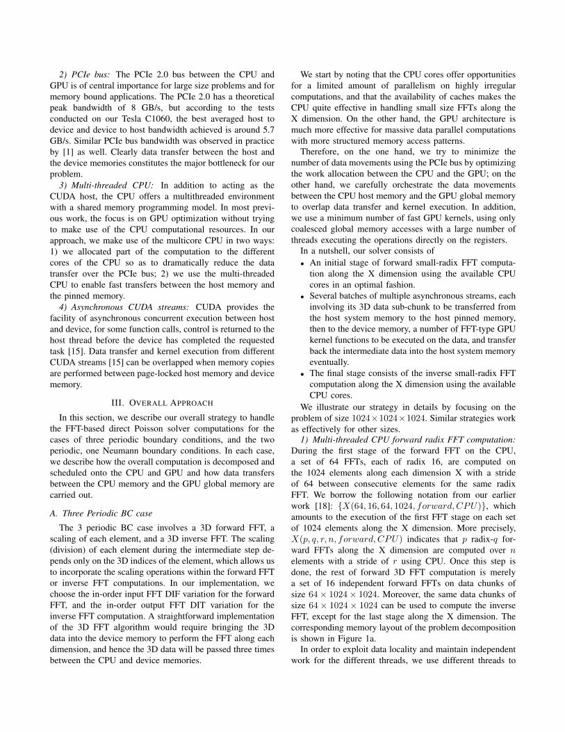
2) PCIe bus: The PCIe 2.0 bus between the CPU andGPU is of central importance for large size problems and formemory bound applications. The PCIe 2.0 has a theoreticalpeak bandwidth of 8 GB/s, but according to the testsconducted on our Tesla C1060, the best averaged host todevice and device to host bandwidth achieved is around 5.7GB/s. Similar PCIe bus bandwidth was observed in practiceby [1] as well. Clearly data transfer between the host andthe device memories constitutes the major bottleneck for ourproblem.

3) Multi-threaded CPU: In addition to acting as theCUDA host, the CPU offers a multithreaded environmentwith a shared memory programming model. In most previ-ous work, the focus is on GPU optimization without tryingto make use of the CPU computational resources. In ourapproach, we make use of the multicore CPU in two ways:1) we allocated part of the computation to the differentcores of the CPU so as to dramatically reduce the datatransfer over the PCIe bus; 2) we use the multi-threadedCPU to enable fast transfers between the host memory andthe pinned memory.

4) Asynchronous CUDA streams: CUDA provides thefacility of asynchronous concurrent execution between hostand device, for some function calls, control is returned to thehost thread before the device has completed the requestedtask [15]. Data transfer and kernel execution from differentCUDA streams [15] can be overlapped when memory copiesare performed between page-locked host memory and devicememory.

III. OVERALL APPROACH

In this section, we describe our overall strategy to handlethe FFT-based direct Poisson solver computations for thecases of three periodic boundary conditions, and the twoperiodic, one Neumann boundary conditions. In each case,we describe how the overall computation is decomposed andscheduled onto the CPU and GPU and how data transfersbetween the CPU memory and the GPU global memory arecarried out.

A. Three Periodic BC case

The 3 periodic BC case involves a 3D forward FFT, ascaling of each element, and a 3D inverse FFT. The scaling(division) of each element during the intermediate step de-pends only on the 3D indices of the element, which allows usto incorporate the scaling operations within the forward FFTor inverse FFT computations. In our implementation, wechoose the in-order input FFT DIF variation for the forwardFFT, and the in-order output FFT DIT variation for theinverse FFT computation. A straightforward implementationof the 3D FFT algorithm would require bringing the 3Ddata into the device memory to perform the FFT along eachdimension, and hence the 3D data will be passed three timesbetween the CPU and device memories.

We start by noting that the CPU cores offer opportunitiesfor a limited amount of parallelism on highly irregularcomputations, and that the availability of caches makes theCPU quite effective in handling small size FFTs along theX dimension. On the other hand, the GPU architecture ismuch more effective for massive data parallel computationswith more structured memory access patterns.

Therefore, on the one hand, we try to minimize thenumber of data movements using the PCIe bus by optimizingthe work allocation between the CPU and the GPU; on theother hand, we carefully orchestrate the data movementsbetween the CPU host memory and the GPU global memoryto overlap data transfer and kernel execution. In addition,we use a minimum number of fast GPU kernels, using onlycoalesced global memory accesses with a large number ofthreads executing the operations directly on the registers.

In a nutshell, our solver consists of• An initial stage of forward small-radix FFT computa-

tion along the X dimension using the available CPUcores in an optimal fashion.

• Several batches of multiple asynchronous streams, eachinvolving its 3D data sub-chunk to be transferred fromthe host system memory to the host pinned memory,then to the device memory, a number of FFT-type GPUkernel functions to be executed on the data, and transferback the intermediate data into the host system memoryeventually.

• The final stage consists of the inverse small-radix FFTcomputation along the X dimension using the availableCPU cores.

We illustrate our strategy in details by focusing on theproblem of size 1024×1024×1024. Similar strategies workas effectively for other sizes.

1) Multi-threaded CPU forward radix FFT computation:During the first stage of the forward FFT on the CPU,a set of 64 FFTs, each of radix 16, are computed onthe 1024 elements along each dimension X with a strideof 64 between consecutive elements for the same radixFFT. We borrow the following notation from our earlierwork [18]: X(64, 16, 64, 1024, forward,CPU), whichamounts to the execution of the first FFT stage on each setof 1024 elements along the X dimension. More precisely,X(p, q, r, n, forward,CPU) indicates that p radix-q for-ward FFTs along the X dimension are computed over nelements with a stride of r using CPU. Once this step isdone, the rest of forward 3D FFT computation is merelya set of 16 independent forward FFTs on data chunks ofsize 64× 1024× 1024. Moreover, the same data chunks ofsize 64× 1024× 1024 can be used to compute the inverseFFT, except for the last stage along the X dimension. Thecorresponding memory layout of the problem decompositionis shown in Figure 1a.

In order to exploit data locality and maintain independentwork for the different threads, we use different threads to

(a) 3D data memory layout (b) CPU and GPU device memory usage

(c) Async CUDA streams applicable to Tesla C1060 (d) block memory copy for one stream

Figure 1: Data decomposition and CPU+GPU memory mapping

work on multiple contiguous rows of 1024 elements: eachthread in our implementation is responsible for carryingout the 64 sets of FFT(16) for a 1024-element row. Uponcompleting the work on 8 rows, the 8 threads move ontoto the next 8 consecutive rows, and so on. Since thereis no dependency between threads, no synchronization isnecessary for correctness and such balanced yet independentworkload distribution makes a very effective use of the cacheby each thread. As a result, we achieve an almost perfectspeed-up by a factor of 8 relative to using just one thread.

2) Asynchronous Streams of Data Transfers and GPUKernels: CUDA allows the use of streams for asynchronousmemory copy and concurrent kernel executions to hide longPCIe bus latency[15]. A stream is a sequence of commandsthat execute in order; different streams may execute theircommands out of order with respect to one another orconcurrently. Asynchronous memory copy has to be carriedout between page-locked host memory and device memory.

In order to make effective use of the asynchronous CPU-GPU memory copy, we organize the remaining FFT com-putations into 4 batches, each consisting of 4 asynchronousstreams where each stream involves a subarray of size64×1024×1024 (0.5 GB). For our running example, stagingpage-locked host memory of size 2GB (0.5GB*4) is allo-

cated to enable asynchronous memory copy, as indicated inFigure 1b. By default, page-locked host memory is allocatedas cacheable and write-combining flag can be used to enablethe memory not being snooped during the transfer across thePCIe bus, which can boost the host to device bandwidthin practice[15]. However, the bandwidth on the oppositetransfer direction is prohibitively slow. So we allocate twoscratch page-locked memory: one with default flag and usingfor device to host transfer and one with write-combining flagand using for host to device transfer. Figure 2 shows onebatch of the complete pipelined execution of multi-threadedCPU (including the main thread and the helper threads) and4 GPU streams (stream 0, 1, 2, 3). Each stream is definedas follows.

• The 3D data subset allocated to each stream is 64 ×1024×1024 in the X, Y and Z dimension respectively.This corresponds to the system host memory layout ver-sus <batch #, stream#>in Figure 1d, which indicates1K × 1K lines of 64 8-byte words with 1024 8-bytesbetween every two lines. These apart elements need tobe packed consecutively in the page-locked memory sothat the following PCIe bus transfer would be effective.The data movement for each data subset is a pipelineof block-wise movement involving a multi-threaded

Figure 2: CPU-GPU Pipeline

CPU memory copy of a large number of 64-elementwords into a consecutive block in the paged-lockedmemory, followed by a PCIe bus transfer. The datamovement from the system host memory to the pinnedhost memory and the data movement from the pinnedhost memory to the device memory is simultaneousas indicated by the two arrows in Figure 1d. Theentire process overlaps PCIe bus transfers with multi-threaded CPU data copy into pinned memory. Due tobandwidth differences of the PCIe bus and the multi-threaded system memory copy, by the time PCIe busis done with the previous sub-chunk, the next sub-chunk will be ready for the asynchronous memory copyinto the device memory. Immediately after we finishthe memory copy for one chunk of 64× 1024× 1024data, we launch the asynchronous kernel calls for thatstream and start the same work of the next chunk of64 × 1024 × 1024 data. Upon the completion of thekernel calls, we make use of asynchronous copy at-tached to the same stream for the copy back. However,due to the limitation of Tesla C1060, there are noconcurrent data transfers back and forth between pinnedmemory and device memory. When we schedule theasynchronous work, we have to schedule the copy backcalls after executing all the copying from the pinnedhost memory to the device memory and their kernelcalls. This asynchronous stream execution is shown inFigure 1c.

• Compute the 3D forward FFT, scaling and 3D inverseFFT computation (except for a partial inverse smallradix FFT along the X dimension) on a chunk of size64 × 1024 × 1024 on the GPU using 7 optimizedkernels. The total execution time of the kernels shouldbe smaller than the total transfer time of 3 streams(3 host to device and 3 device to host, Figure 1c);otherwise, one or more of the streams’ memory transfer

back needs to be held back until the completion of itskernel. This is illustrated in Figure 1c. Since we want toachieve a high PCIe bus bandwidth, the kernels have toexecute as fast as well. Once the data is loaded onto theGPU device memory, we can use techniques similar tothose introduced in our previous work [18] to computethe FFT of each subarray of size 64× 1024× 1024. Inparticular, the X-dimensional radix-64 forward FFT andinverse FFT are included in the Y and Z dimensionalFFT computation kernels to avoid additional globalmemory accesses. Moreover, effective shared memorytranspose strategies are used to guarantee no bankconflicts. An intermediate global memory (shared by4 streams due to their sequential execution of kernels)is introduced for smaller strides between consecutiveglobal memory accesses when multiple Z dimensionalcomputation kernels are involved (Figure 1b), withoutlimiting the maximum number of concurrent streams.The scaling step is included in the last step of theforward FFT and the first step of the inverse FFT withthe scalars computed using bit-reversed indices.As a result, the GPU kernels can be defined by thefollowing computations:

– X(8, 8, 8, 64), Y (32, 32, 32, 1024), forward– X(8, 8, 1, 8), Y (32, 32, 1, 32), forward)– Z(32, 32, 32, 1024), forward– Z(32, 32, 1, 32), forwardscaling,GPU)Z(32, 32, 1, 32), inverse

– Z(32, 32, 32, 1024), inverse– X(8, 8, 1, 8), Y (32, 32, 1, 32), inverse– X(8, 8, 8, 64), Y (32, 32, 32, 1024), inverse

Note that all the arithmetic computations are carried outon register contents, all global memory transfers involvecoalesced memory access, and transpose computationsuse shared memory without any bank conflicts. There-fore, we complete the 64× 1024× 1024 forward FFT,scaling and inverse FFT using 7 kernels.

• Once the kernels are completed, we perform block-wise asynchronous memory copies from the devicememory to the pinned host memory and then to thesystem host memory for each stream. CPU functioncalls are synchronous in nature, and CPU memorycopy back calls have to wait for the completion of theasynchronous GPU-to-CPU memory copy for that datachunk (Figure 2).

3) Multi-threaded CPU inverse radix FFT computation:This step is similar to the very first step to computepartial FFTs along the X dimension using the 8 coresof the CPU. Such a computation can be described byX(64, 16, 64, 1024, inverse, CPU)

IV. 2 PERIODIC 1 NEUMANN POISSON SOLVER

A. Algorithm

Suppose our 3D input data is of size IxJxK. The 2 periodic1 Neumann BC case involves K sets of 2D forward FFTs,each of size IxJ, followed by IxJ sets of tridiagonal linearsystems, each of size KxK, followed by K sets of 2Dinverse FFT of size IxJ. We have a similar computationdecomposition and distribution on the CPU and GPU, asthe three periodic BC case.

B. Strategy

We illustrate our strategy for the case of 1024× 1024×1024 , and examine in some detail how the work is allocatedbetween the CPU and the GPU. The same strategy worksfor other problem sizes as we demonstrate later. The overallapproach can be described as follows.

• As before, the first step is carried out on theCPU, and partially computes the forward FFT alongthe X dimension using the scheme described by:X(64, 16, 64, 1024, forward,CPU), i.e., 64 FFTseach of radix-16, stride-64, for each 1024-element row.

• Launch a set of asynchronous streams involving mem-ory copy and each of the streams performs the follow-ing computations of data size 64×1024×1024 runningon the GPU:

– Compute the forward radix-64 FFTalong the dimension X as described by:X(1, 64, 1, 64, forward,GPU) and theforward FFTs along the Y dimension:Y (1, 1024, 1, 1024, forward,GPU)

– Using Thomas’ algorithm, solve thetridiagonal linear systems of equationsZ(1024, tridiagonal solver,GPU)

– Compute the inverse FFT along the Y dimension:Y (1, 1024, 1, 1024, inverse,GPU) and the in-verse radix-64 FFT along the X dimension:X(1, 64, 1, 64, inverse,GPU)

• After the GPU completes the execution of allthe kernels and the intermediate results are

written back in the CPU main memory, weexecute the following inverse FFT computation:X(64, 16, 64, 1024, inverse, CPU) using the 8CPU cores.

Note that, once a chunk is loaded into the GPU globalmemory, we ensure a fast GPU execution by minimizingthe number of global memory accesses, all of which areguaranteed to be coalesced. Similar as in the 3D periodiccase, the X dimensional radix-64 forward and inverse FFTscan be included in the 2 kernels within the Y dimensionalsize 1024 forward and inverse FFTs. Such a GPU allocationallows us to use 64 CUDA threads to process the Y and/orZ dimensional computations in a vector-wise manner, whichnaturally guarantee coalesced global memory access of alldata.

CUDA streams are employed to combine the CPU andGPU work using asynchronous memory copy and kernelexecutions in a similar way to what we did for the 3 periodicBC case: 4 streams achieve typically a very good PCIebandwidth (around 5GB/s) in our experiments.

C. Arithmetic Precision

When it comes to GPU performance, single precisionfloating point arithmetic enjoys significant benefits over dou-ble precision arithmetic[7]. Since single precision floatingpoints use half of the memory space of double precisionfloating points, single precision implementations potentiallysave half of the memory transfer time, for the PCIe busand for the global memory accesses. Also, single precisioncomputations are faster than double precision computationsin many architectures, including the Tesla C1060 we areusing. An important characteristic of our algorithm is tosecure a 2nd order convergence, and hence if we make thegrid twice as dense, we expect the accuracy to double. In ourexperiments, double precision arithmetics can easily guar-antee such property at the expense of slower computationtime, while pure single precision implementations showeda relatively larger error when compared to the discretizedanalytic function used in our tests. And due to the slow PCIpeak bandwidth and fast GPU kernels, these two variationsshow almost the same performance in our experiments.

To achieve high performance while ensuring the 2nd orderconvergence, we make use of a precision boost for theintermediate data. Through careful examination, we noticethat the step that most affects the precision is the divisionstep in the forward elimination stage: m = a[i]/b[i − 1].More specifically, the error becomes large when b[i − 1] issmall. Note that in our implementation, the b[i−1] is storedand updated as we iterate along i. Hence we use doubleprecision to store the b[i−1] values and immediately relatedvariables, and then cast the results back into single floatingpoints. By using this trick, we can avoid the substantialoverhead of converting the entire data into double precisionwhile achieving the desired accuracy.

Table I: Basic Parameters of Tesla C1060 (SM: Streaming Multiprocessor;SP: Streaming Processor)

# ofSMs

# ofSPs

# ofRegisters

SharedMem.

GlobalMem.

NvccCufft

Tesla C1060 30 8 16K 16KB 4GB 3.2.16

Table II: CPU configuration

CPU Freq. Cores Sys. Mem. GCC FFTWXeon X5560 2.80GHz 2 quad-core 24 GB 4.7.2 3.3.2

V. PERFORMANCE

In this section, we present a summary of the performancetests that have been conducted on our CPU-GPU platform.Our CPU consists of two Quad-Core Intel Xeon X5560, eachQuad-core with an 8 MB L3 cache, such that the total mainmemory is of size 24 GB . Our GPU card is an NVIDIATesla C1060 GPU, and data transfer between the CPU mainmemory and the GPU device memory is through PCIe 2.0bus. Tables I and II provide more detailed information aboutour GPU and CPU configurations.

In our tests, the problem size is a power-of-two in eachof the three dimensions. We use input sizes that cannot beaccommodated by the device memory alone (in particular,we would not be able to run CUFFT on the sizes that shouldin principle fit the device memory).

Since the core of our algorithms is based on either3D or 2D FFT computations, we use the following well-known formula to estimate the FFT GFLOPS performance,assuming that the execution time of a one-dimensional FFTon data size NX is t seconds:

GFLOPS =5 ·NX · log2 (NX) · 10−9

t(4)

At some point, we compare the performance of our FFTimplementations against implementations obtained by thesingle-precision multi-threaded Single Instruction MultipleData (SIMD) code enabled version FFTW library [6][4][5](2D or 3D). We use “MEASURE” patient level whengenerating the execution plan since using a more rigorouspatient level will take over 8 hours to generate the executionplan for the problem sizes we are dealing with.

A. The Case of Three Periodic Boundary Conditions

Our three periodic BC Poisson solver consists of a for-ward 3D FFT, a scaling (division) step for each elementof the intermediate 3D array, followed by an inverse 3DFFT. Therefore, the number of GFLOPS achieved by ouralgorithm can simply be calculated based on the 3D FFTGFLOPS formula. Since we do not include the intermediatescaling step in our estimate, we under-estimate the perfor-mance of our algorithm. Specifically, if the total executiontime on a 3D data set of size NX×NY×NZ is t seconds, then

its GFLOPS can be measured using the standard formula:

GFLOPS =2· 5·NX ·NY ·NZ ·[log2 (NX ·NY ·NZ)]·10−9

t(5)

The coefficient 2 in the above formula captures the forwardand the inverse FFT. Figure 3a illustrates the GFLOPSperformance of our Poisson solver and ourcombined 3Dforward and inverse FFTs. We have also included the per-formance of the 3D forward and inverse FFTW running onour CPU as a point of reference. As can be seen from thefigure, we were able to achieve more than 55 GFLOPS forall data sizes for our Poisson solver and for our combinedforward and inverse FFTs. The best that we were able toachieve using FFTW is around 20 GFLOPS.

As stated in the introduction, and as illustrated in theabove figure, our performance is substantially better thanthose reported in the most recent related works of [1] and[11].

We now compare the PCIe transfer time to the totalPoisson solver time. Figure 3c shows the ratio of the bestpossible achievable PCIe transfer time and the total solvertime for several 3D grid sizes. The best achievable bus trans-fer time is computed by simply moving the correspondingdata from main memory to the GPU global memory, andimmediately writing it back to the CPU main memory. Ascan be seen from this figure, more than 50% of the totalsolver time is consumed in moving the data once betweenthe CPU main memory and the device memory. The bestprevious algorithm for the 3D forward FFT moved the datatwice, and hence incur a substantial overhead compared toour algorithm, even without including the scaling and theinverse FFT steps. Figure 3c also shows the ratio of thetotal GPU time of our solver versus the entire solver time.The total GPU time starts from the moment the CPU beginsto copy data from the system host memory to the pinnedhost memory and ends at the moment that all the GPUcomputations are completed and the output is stored backin the original system host memory. As we can see fromthe figure for the 3 periodic BC case, the GPU related time(which in fact results from one round of PCIe bus memorytransfer) represents around 60%-70% of the total runtime.

We now turn our attention to our CPU partial FFTcomputation along the X dimension. The allocation of thethis computation to the CPU has enabled us to perform thewhole computation with just one transfer of the 3D dataover the PCIe bus. Figure 4 demonstrates the scalability ofthe CPU implementation relative to the number of threadsfor different sizes. On the other hand, Figure 3c provides theratio of CPU part radix FFT runtime and the best achievablePCIe bus bandwidth on the same data size. Therefore with4 or more threads, the execution time of this part of thecomputation is substantially less than the best achievabletransfer time of the 3D data between the CPU main memoryand the GPU global memory. In fact, with 8 threads, the

(a) 3 Periodic BC Performance Comparison (b) 2 Periodic 1 Neumann BC Performance Comparison

(c) Ratios of PCIe transfer time to solver time, GPU solver time,for both types of boundary conditions

(d) CPU radix FFT runtime vs. PCI transfer time

(e) 3 Periodic BC BW vs # of Threads (f) 2 Periodic 1 Neumann BC BW vs # of Threads

Figure 3: Performance Evaluation Summary

CPU radix-FFT time is around 40% of the best possibledata transfer time over the PCIe bus.

We now take a closer look at the PCIe bandwidth achievedby our solver and at how we were able to overlap the execu-

tion of the GPU kernels with the CPU-GPU asynchronousmemory copy enabled by the asynchronous CUDA streams.

We evaluate the effective PCIe bandwidth using Formula

Table III: Arithmetic Accuracy of 3D Periodic BC Solver

Data size Our Solver Using FFTW512× 1024× 1024 0.000028 0.0000281024× 512× 1024 0.000012 0.0000131024× 1024× 512 0.000028 0.0000281024× 1024× 1024 0.000011 0.0000122048× 1024× 512 0.000024 0.0000242048× 512× 1024 0.000008 0.000008

Figure 4: CPU radix FFT runtime scalability

6:BW =

2 · 8 ·NX ·NY ·NZ · 10−9

t(6)

where 8 in the formula is due to the fact that the numberof bytes occupied by each single floating point complexelement is 8 and 2 indicates moving the data from theCPU to the GPU and then back to the CPU.The timet used in the above formula excludes the CPU runtimefor the first stage of X dimensional forward FFT and thelast stage of X dimensional inverse FFT. The time t startsfrom the momentthat the CPU begins to copy data fromthe system host memory to the pinned memory for theasynchronous memory copy, and ends at the moment thatall the complete results are copied back into the systemhost memory. Figure 3e demonstrates the achieved PCIebus bandwidth when different numbers of threads are usedwhen copying data from the system host memory to thepinned memory in blocks. We use multi-threading memorycopy for each block, followed by an immediate CPU to GPUasynchronous memory copy call for that block.

Finally, Table III shows the maximum absolute differencebetween the results obtained by our solver and the dis-cretized the analytic function cos(2πx) ·sin(2πy) ·cos(2πz)on the grid used to generate our input data. Our solverdemonstrates similar accuracy compared to the FFTW li-brary single precision.

B. The Two-Periodic and One-Neumann BC Case

As described before, for the problem of size NX×NY ×NZ, the two periodic and one Neumann BC case Poisson

Table IV: Arithmetic Accuracy of 2 Periodic 1 Neumann BC Solver

Data size Our Solver Using FFTW512× 1024× 1024 0.000008 0.0000061024× 512× 1024 0.000008 0.0000071024× 1024× 512 0.000006 0.0000061024× 1024× 1024 0.000008 NA2048× 512× 1024 0.000008 NA2048× 1024× 512 0.000005 NA

Solver consists of NZ number of 2D forward FFTs, eachof size NX×NY , NX×NY tridiagonal linear systems withmatrix size NZ×NZ, and NZ number of 2D inverse FFTs,each of size NX×NY . We conduct a similar experimentaltests as those carried out for 3 periodic BC case; however,we employ a GFLOPS formula that is appropriate for thecorresponding computations. The number of GFLOPS nowconsist of two components: the 2D FFT computations, andthe 1D tridiagonal solvers.

The 2D FFT or IFFT component can be easily capturedas follows. If the execution time of 2D FFT or IFFT on dataof size NX×NY is t seconds, then

GFLOPS =5·NX ·NY ·[log2 (NX ·NY )]·10−9

t(7)

The number of GFLOPS needed to solve the tridiagonallinear system of size N is 8N , and hence the total GFLOPSformula for the 2 periodic (say, the X and Y dimensions) 1Neumann (say, Z dimension) BC is the following:

GFLOPS =NX ·NY ·NZ ·[10·log2 (NX ·NY ) + 8]·10−9

t(8)

The total GFLOPS performance of our Poisson solver forthis case is shown in Figure 3b. As can be seen from thisfigure, we were able to achieve over 40 GFLOPS for all theproblem sizes tested. We now compare our implementationagainst an implementation that uses a single-precision FFTWlibrary to compute the 2D FFTs and an optimized Thomasalgorithm based tridiagonal solver. The tridiagonal solveris customized to the Poisson Solver for better performanceand is essentially a double precision solver with single-precision input and output data. Double precision is neces-sary to achieve second order accuracy. Intermediate memorytranspositions were needed between the FFT and the tridi-agonal solver to guarantee the efficiency of both the FFTWlibrary and the tridiagonal solver; however, we excludethe transposition time when evaluating the performance toindicate a best possible achievable performance using thestandard library. Figure 3b demonstrates the comparisonbetween the two implementations. As we can see, our solverdemonstrates superior performance in all cases even if wejust compare to the 2D FFTW library to our solver, whichincludes a tridiagonal solver.

On the other hand, in terms of the effective PCIe band-width, we still use of the same Formula 6 since the sametype of data movements are occurring as before.

Due to the sufficient number of concurrent CUDAstreams, and relatively smaller total time of the GPU kernelsof each stream, we were able to better hide the GPU kernelexecutions which yields a higher effective PCIe transferbandwidth. As we can observe from Figure 3f, around 5GB/s effective PCIe bandwidth is achieved for all data sizesby using 4 or 8 CPU threads for memory copy.

Finally, we compare in Table IV the accuracy using oursingle precision solver on the discretized analytic functionsin(2πx + π

10 ) · cos(2πy) · cos(2πz) on the grid with theprecision boost step against the naive standard methodimplementation with single precision FFTW and doubleprecision tridiagonal solver. Due to the additional memoryused for intermediate array transposition, some larger sizedproblems could not be completed. As can be seen from thetable, our solver achieves similar accuracy as the FFTW sin-gle precision algorithm and the double precision tridiagonalsolver.

VI. CONCLUSION

We presented in this paper a new strategy to map an FFT-based direct Poisson solver on a CPU-GPU heterogeneousplatform, which optimizes the problem decomposition usingboth the CPU and the GPU. The new approach effectivelypipelines the PCIe bus transfer and GPU work, almostentirely overlapping the CPU-GPU memory transfer timeand the GPU computation time. Experimental results over awide range of grid sizes have shown very high performance,both in terms of the number of floating point operationsper second and the effective PCIe bus memory bandwidth.The performance numbers are superior to those that wereachieved in previous related work.

ACKNOWLEDGMENT

This work was partially supported by an NSF PetaAppsaward, grant OCI0904920, the NVIDIA Research Excel-lence Center at the University of Maryland, and by an NSFResearch Infrastructure Award, grant number CNS 0403313.

REFERENCES

[1] Y. Chen, X. Cui, and H. Mei. Large-scale FFT on GPUclusters. In Proceedings of the 24th ACM InternationalConference on Supercomputing, ICS ’10, pages 315–324,New York, NY, USA, 2010. ACM.

[2] J. Cooley and J. Tukey. An algorithm for the machine calcula-tion of complex Fourier series. Mathematics of Computation,19(90):297–301, 1965.

[3] Y. Dotsenko, S. Baghsorkhi, B. Lloyd, and N. Govindaraju.Auto-tuning of fast Fourier transform on graphics processors.In Proceedings of the 16th ACM symposium on Principles andpractice of parallel programming, PPoPP ’11, pages 257–266,New York, NY, USA, 2011. ACM.

[4] M. Frigo. A fast Fourier transform compiler. SIGPLAN Not.,34(5):169–180, May 1999.

[5] M. Frigo and G. Johnson. The FFTW website, 2012. http://www.fftw.org.

[6] M. Frigo, Steven, and G. Johnson. The design and imple-mentation of FFTW3. In Proceedings of the IEEE, pages216–231, 2005.

[7] D. Goddeke and R. Strzodka. Cyclic reduction tridiagonalsolvers on GPUs applied to mixed-precision multigrid. IEEETrans. Parallel Distrib. Syst., 22(1):22–32, Jan. 2011.

[8] N. K. Govindaraju, S. Larsen, J. Gray, and D. Manocha. Amemory model for scientific algorithms on graphics proces-sors. In Proceedings of the 2006 ACM/IEEE conference onSupercomputing, SC ’06, New York, NY, USA, 2006. ACM.

[9] N. K. Govindaraju, B. Lloyd, Y. Dotsenko, B. Smith, andJ. Manferdelli. High performance discrete Fourier trans-forms on graphics processors. In Proceedings of the 2008ACM/IEEE conference on Supercomputing, SC ’08, pages2:1–2:12, Piscataway, NJ, USA, 2008. IEEE Press.

[10] L. Gu, X. Li, and J. Siegel. An empirically tuned 2D and3D FFT library on CUDA GPU. In Proceedings of the 24thACM International Conference on Supercomputing, ICS ’10,pages 305–314, New York, NY, USA, 2010. ACM.

[11] L. Gu, J. Siegel, and X. Li. Using GPUs to compute large out-of-card FFTs. In Proceedings of the international conferenceon Supercomputing, ICS ’11, pages 255–264, New York, NY,USA, 2011. ACM.

[12] R. Mittal and G. Iaccarino. Immersed boundary methods. InAnn. Rev. Fluid Mech. 37, pages 239–261, 2005.

[13] A. Nukada and S. Matsuoka. Auto-tuning 3-D FFT libraryfor CUDA GPUs. In Proceedings of the Conference on HighPerformance Computing Networking, Storage and Analysis,SC ’09, pages 30:1–30:10, New York, NY, USA, 2009. ACM.

[14] A. Nukada, Y. Ogata, T. Endo, and S. Matsuoka. Bandwidthintensive 3-D FFT kernel for GPUs using CUDA. In Proceed-ings of the 2008 ACM/IEEE conference on Supercomputing,SC ’08, pages 5:1–5:11, Piscataway, NJ, USA, 2008. IEEEPress.

[15] NVIDIA Corporation. NVIDIA CUDA C programmingguide, 2011.

[16] B. C. Sidney. Fast Fourier Transforms. Appendix 1:FFT flowgraphs, 2012. http://cnx.org/content/m16352/latest/?collection=col10550/1.20.

[17] J. Wu and J. JaJa. An optimized FFT-based direct Poissonsolver on CUDA GPUs. IEEE Trans. Parallel Distrib. Syst.To appear.

[18] J. Wu and J. JaJa. Optimized strategies for mapping three-dimensional FFTs onto CUDA GPUs. In Innovative ParallelComputing (INPAR). IEEE Press, 2012.