High Performance Multivariate Visual DataExploration for Extremely Large Data

Oliver Rubel1,5,6, Prabhat1, Kesheng Wu1, Hank Childs2, Jeremy Meredith3, Cameron G.R. Geddes4,Estelle Cormier-Michel4, Sean Ahern3, Gunther H. Weber1, Peter Messmer7, Hans Hagen6,

Bernd Hamann1,5,6 and E. Wes Bethel1,5

Abstract—One of the central challenges in modern scienceis the need to quickly derive knowledge and understandingfrom large, complex collections of data. We present a newapproach that deals with this challenge by combining andextending techniques from high performance visual data analysisand scientific data management. This approach is demonstratedwithin the context of gaining insight from complex, time-varyingdatasets produced by a laser wakefield accelerator simulation.Our approach leverages histogram-based parallel coordinatesfor both visual information display as well as a vehicle forguiding a data mining operation. Data extraction and subsettingare implemented with state-of-the-art index/query technology.This approach, while applied here to accelerator science, isgenerally applicable to a broad set of science applications, andis implemented in a production-quality visual data analysisinfrastructure. We conduct a detailed performance analysis anddemonstrate good scalability on a distributed memory Cray XT4system.

I. INTRODUCTION

This work focuses on combining and extending two differ-ent but complementary technologies aimed at enabling rapid,interactive visual data exploration and analysis of contempo-rary scientific data. To support highly effective visual dataexploration, knowledge discovery and hypothesis testing, wehave adapted and extended the concept of parallel coordinates,in particular binned or histogram-based parallel coordinates,for use with high performance query-driven visualization ofvery large data. In the context of visual data explorationand hypothesis testing, the parallel coordinates display andinteraction mechanism serves multiple purposes. First, it actsas a vehicle for visual information display. Second, it serves asthe basis for the interactive construction of compound Boolean

1. Computational Research Division, Lawrence Berkeley National Laboratory,One Cyclotron Road, Berkeley, CA 94720, USA.2. Lawrence Livermore National Laboratory, 7000 East Avenue, Livermore,CA 94550.3. Oak Ridge National Laboratory, P.O. Box 2008, Oak Ridge, TN 37831,USA.4. LOASIS program of Lawrence Berkeley National Laboratory, One Cy-clotron Road, Berkeley, CA 94720, USA.5. Institute for Data Analysis and Visualization (IDAV) and Department ofComputer Science, University of California, Davis, One Shields Avenue,Davis. CA 95616, USA.6. International Research Training Group “Visualization of Large and Unstruc-tured Data Sets – Applications in Geospatial Planning, Modeling, and En-gineering,” Technische Universitat Kaiserslautern, Erwin-Schrodinger-Straße,D-67653 Kaiserslautern, Germany.7. Tech-X Corporation, 5621 Arapahoe Ave. Suite A, Boulder, CO 80303.

data range queries. These queries form the basis for subsequent“drill down” or data mining actions. To accelerate data mining,we leverage state-of-the-art index/query technology to quicklymine for data of interest as well as to quickly generatemultiresolution histograms used as the basis for the visualdisplay of information. This combination provides the abilityfor rapid, multiresolution visual data exploration.

We apply this new technique to large, complex scientificdata created by a numerical simulation of a laser wakefieldparticle accelerator. In laser wakefield accelerators, particlesare accelerated to relativistic speeds upon being “trapped”by the electric fields of plasma density waves generated bythe radiation pressure of an intense laser pulse fired into theplasma. These devices are of interest because they are ableto achieve very high particle energies within a relatively shortamount of distance when compared to traditional electromag-netic accelerators. The VORPAL [1] simulation code is usedto model experiments, such as those performed at the LOASISfacility at LBNL [2], and is useful in helping to gain deeperunderstanding of phenomena observed in experiments, as wellas to help formulate and optimize the methodology for futureexperiments.

Laser wakefield simulations model the behavior of individ-ual particles as well as the behavior of the plasma electric andmagnetic fields. Output from these simulations can becomequite large: today’s datasets, such as the ones we studyhere, can grow to be on the order of 200GB per timestep,with the simulation producing ≈ 100 timesteps. The scientificchallenge we help address in this study is first to quickly findparticles that have undergone wakefield acceleration, then tracethem through time to understand acceleration dynamics, andperform both visual and quantitative analysis on the set ofaccelerated particles.

One scientific impact of our work is that we have vastlyreduced the duty cycle in visual data exploration and mining.In the past, accelerator scientists would perform the “tracebackwards” step using scripts that performed a search at eachtimestep for a set of particles. Runtimes for this operationwere on the order of hours. Using our implementation, thoseruntimes are reduced from hours to seconds.

The specific new contributions of this work are as follows:• We present a novel approach for quickly creating

histogram-based parallel coordinates displays. These dis-plays serve to convey information as well as the interfacefor the interactive construction of compound, multivariate

Boolean range queries. The new approach leverages state-of-the-art index/query technology to achieve very favor-able performance rates.

• We apply this new approach to solve a challenging scien-tific data understanding problem in accelerator modeling.This new approach performs particle tracking in a fewseconds as compared to hours when using a naive script.

• We examine and report the performance of our approachusing a modern HPC platform on a very large (≈1.5TB)and complex scientific dataset. We demonstrate that ourapproach has excellent scalability characteristics on adistributed memory Cray XT4 system.

The rest of this paper is organized as follows. First, wereview relevant background work in Section II, which cov-ers a diverse set of topics in visual information display,index/query technology, and high performance visual dataanalysis software architectures. Next in Section III, we presentthe architecture and implementation of our approach. Thisapproach is then applied to solve a challenging scientific dataunderstanding problem in the field of laser wakefield acceler-ator modeling in Section IV. We evaluate the performanceof our system and present performance results in SectionV. Finally, we conclude in Section VI with a summary andsuggestions for future work.

II. RELATED WORK

A. Information Display – Parallel Coordinates

Parallel coordinates, proposed by Inselberg [3] and Weg-man [4], are a common information visualization techniquefor high-dimensional data sets. In parallel coordinates, eachdata variable of a multivariate dataset is represented by oneaxis. The parallel coordinates plot is constructed by drawing apolyline connecting the points where a data record’s variablevalues intersect each axis. This type of plot is expensivein the sense that many pixels are required to represent asingle data record. In this form of display, there is substantialdata occlusion by the many polylines required to display allrecords from a large dataset. An overview of modern parallelcoordinates is provided in [5], [6].

Fua et al. [7] proposed using hierarchical parallel coordi-nates, based on hierarchical clustering, to create a multireso-lution view of the data that enables data exploration at varyinglevels of detail. Johannson et al. [8] used clustering to deter-mine the inherent structure of data, and displayed that structurewith high-precision textures using different texture transferfunctions. Novotny then used a binning algorithm based on ak-means clustering approach for creating an aggregate parallelcoordinates visualization [9]. All these approaches are well-suited for presenting static data, but are not well suited fortime-varying data since defining temporally consistent clustersis non-trivial and computationally expensive.

Our histogram-based parallel coordinates approach extendsthe work of Novotny and Hauser [10], who proposed usingbinned parallel coordinates as an output-oriented (rendering)approach. The main limitation of this approach is that in

order to achieve interactive rendering speed, their methodprecomputes all possible 2D histograms with a fixed resolutionof 256× 256 and uniform, equal-sized histogram bins. Toimplement different level-of-detail views, bins in the pre-computed histograms are merged, reducing the number of binsby half in each drill down step. While this strategy is efficient,it has several limitations. First, it does not allow for smoothlydrilling into finer-resolution views of the data. Second, itsupports presentation of binned views of the entire dataset,but does not support user-defined data subsetting. Finally,the fixed 256× 256 histogram resolution exhibits significantaliasing when zooming in on narrow variable ranges in theparallel coordinates plot. Their approach uses binned parallelcoordinates for “context views” and traditional, polyline-basedparallel coordinates for “focus views.” These focus views maystill contain a substantial number of data records and willsuffer from extensive occlusion as a result.

B. High Performance Index/Query for Data Mining

The data access patterns for data mining and analysisapplications tend to be markedly different from those fortransaction-based applications. Transaction-based applicationstend to read and then update records in a database. In contrast,data mining and analysis applications tend to be read-only intheir access pattern. The database indexing technology that isbest suited for this type of data access is known as the bitmapindex [11], [12]. The core idea of a bitmap index is to usea sequence of bits to mark the positions of records satisfyingcertain conditions. Searching bitmap indices for data recordsthat match a set of range conditions is performed efficientlyusing Boolean operations on bit vectors.

In uncompressed form, such bitmap indices may requiretoo much space for variables with many distinct values, suchas particle position or momentum. Several techniques havebeen proposed to improve the efficiency of the bitmap indexeson such variables [13], [14]. We make use of a bitmapindex software called FastBit [15]. It implements the fastestknown bitmap compression technique [16], [17], and has beendemonstrated to be effective in a number of data analysisapplications [18], [19]. In particular, it has a number ofefficient functions for computing conditional histograms [20],which are crucial for this work. Furthermore, FastBit indicesare relatively small compared to popular indices such as B-trees [16, Fig. 7] and can be constructed much faster thanothers [21, Fig. 12]. Bitmap indices are well-known for theireffectiveness on data with relatively small number of distinctvalues, such as gender. FastBit indices have been demonstratedto be very efficient also for data with a large number of distinctvalues through its unique compression [14] and binning [22].

When a variable has a large number of distinct values thecorresponding FastBit index is typically on a binned versionof the data, where a bit is 1 if the value of a record fallsin a particular bin. In this case, the number of 1s in abitmap corresponding to a bin is the number of records inthe bin. This provides an efficient method for computing ahistogram [20]. FastBit offers a number of different options

for creating bitmap bins. When composing range queries,users typically specify conditions with relatively low-precisionvalues, such as pressure less than 1 ∗ 10−5 or momentumgreater than 2.5 ∗ 108. The constant 1 ∗ 10−5 is said to have1-digit precision, and the constant 2.5 ∗ 108 to have 2-digitprecision. FastBit can build indices with bin boundaries withany user-specified precision so that all queries involving low-precision boundaries are answered accurately with index only.These features make FastBit uniquely suitable for this work.

C. High Performance Query-Driven Visualization

The combination of high performance index/query withvisual data exploration tools was described by Stockinger etal. [23] using the term “Query-driven visualization.” That workfocuses on comparing the performance of such a combinationwith state-of-the-art, tree-based searching structures that formthe basis for a widely-used isocontouring implementation.Their work shows that this approach outperforms tree-basedsearch structures for scalar variables, and also points out thatall tree-based index/search structures are not practical forlarge, multivariate datasets since they suffer from the “Curse ofDimensionality” [24]. The basic idea there is that storage com-plexity grows exponentially as one adds more and more searchdimensions (e.g., more variables to be indexed/searched).

These concepts were later extended to the analysis ofmassive collections of network traffic data in two relatedworks. First, the notion of performing network traffic analysisusing statistics (e.g., histograms) rather than raw data ledto a methodology that enabled exploration and data miningat unprecedented speed [18]. That study showed using theseconcepts to rapidly detect a distributed scan attack on a datasetof unprecedented size – 2.5 billion records. There, usersare presented with an interface consisting of histograms ofindividual variables, and then they formulate a complex queryvia a process that is essentially a histogram “cross product.”The process of data mining was subsequently acceleratedthrough a family of algorithms for computing conditionalhistograms on SMP parallel machines [25].

D. High Performance Visual Data Analysis

Childs et al. [26] demonstrated a data processing andvisualization architecture that is capable of scaling to extremedataset sizes. This software system, VisIt [27], has been shownto scale to tens of billions of data points per timestep and runsin parallel on nearly all modern HPC platforms. In reference toour work, VisIt employs a contract-based communication sys-tem that allows for pipelining and I/O optimization, reducingunnecessary processing and disk access. It is this extensiblecontract system that we utilize to generate histograms forvisual data exploration. A specific optimization that we employis VisIt’s concept of a set of Boolean range queries. This set iscommunicated between data processing modules in an out-of-band fashion, allowing downstream filters to limit the scopeof work of upstream filters.

VisIt’s remote visualization capability crosses several inde-pendent axes. In addition to parallelization of data fetching,

Data incl. Bitmap Index

2D Histograms

Request Histograms

Context

Focus

2D Histograms

Data Operator

FastBit

Define Condition

Selected DataThresholds / Id's

Select and TracePlot

Fig. 1. An overview of the major components and data flow paths inour implementation. Large-scale scientific data and indexing metadata areinput via a parallel I/O layer, which allows us to achieve high levels ofperformance and parallel efficiency. We use an API at the I/O layer toperform parallel computation of multidimensional histograms as well asdata subsetting. Results of those computations are used downstream in thevisualization application for presenting information to the user and in supportof interactive data mining actions.

VisIt also performs data extraction and calculation entirely inparallel. Finally, rendering may be done in serial or parallel,depending on the data load. If the resultant geometry is smallenough, it is collected at the HPC side and shipped across thenetwork to the user’s desktop for GPU-based rendering. How-ever, if the geometry is too large for interactive display on asingle GPU, VisIt employs sort-last rendering and compostingon the HPC system, with the resultant pixels shipped acrossthe network to the user’s display. The model described herehas many parallels to remote visualization architectures suchas those in ParaView [28] and EnSight [29].

III. SYSTEM DESIGN

Figure 1 shows a high-level view of the components anddata flow in our implementation. Raw scientific data, whichis produced by simulation or experiment, is augmented bythe computation of indexing data. In our case, this step isperformed outside the visual data analysis application as aone-time preprocessing, and our implementation uses FastBit[15] for creating index structures. The data sizes are describedin more detail in Section IV and V.

After the one-time preprocessing step, our implementationuses FastBit at the data-loading portion of the pipeline toquickly compute histograms in parallel and to perform high-performance data subsetting/selection based upon multivari-ate thresholds or particle identifier (Section III-B). Thesehistograms serve as the basis for the visual presentation offull-resolution and subset views of data vis-a-vis parallelcoordinates plots (Section III-A). In our implementation, thecomputational complexity of rendering parallel coordinatesplots – both context and focus views – is a function ofhistogram resolution, not the size of the underlying data.Therefore, our approach is particularly well-suited for appli-cation to extremely large data, which we present in SectionIV.

A. Histogram based Parallel Coordinates

Parallel coordinates provide a very effective interface fordefining multi-dimensional queries based on thresholding.Using sliders attached to each axis of the parallel coordinates

a) b)

c) d)

Fig. 2. Comparison of different parallel coordinate renderings of a subset ofa 3D laser wakefield particle acceleration dataset consisting of 256,463 datarecords and 7 data dimensions. a) Traditional line based parallel coordinates.b) High-resolution, histogram-based parallel coordinates with 700 bins perdata dimension. c) Same as in b, but using a lower gamma value g definingthe basic brightness of bins. d) Same rendering as in b but using only 80 binsper data dimension. When comparing a and b, we see that the histogram-based rendering reveals many more details when dealing with a large numberof data records. As illustrated in c, by lowering gamma we can then reducethe brightness of the plot and even remove sparse bins, thereby producinga plot that focuses on the main, dense features of the data. By varying thenumber of bins we can then create renderings at different levels of detail.

plot, a user defines range thresholds in each displayed dimen-sion. By rendering the user-selected data subset (the focusview) in front of a parallel coordinates plot created from theentire data set (or in many cases a subset of it) (the contextview), the user receives immediate feedback about generalproperties of the selection. Data outliers stand out visually assingle or small groups of lines diverging from the main datatrends. Data trends appear as dense groups of lines (brightcolored bins in our case). A quick visual comparison of thefocus and context views helps to convey understanding aboutsimilarities and differences between the two.

In practice, parallel coordinates have disadvantages whenapplied to very large datasets. First, each data record isrepresented with a single polyline that connects each of theparallel coordinates axes. As data size increases, the plotbecomes more cluttered and difficult to interpret. Also, datarecords drawn later will occlude information provided by datarecords drawn earlier. Worst of all is that this approach hascomputational and rendering complexity that is proportionalto the size of the dataset. As data sizes grow ever larger, theseproblems become intractable.

To address these problems, we employ an efficient renderingtechnique based on two-dimensional (2D) histograms. Ratherthan viewing the parallel coordinates plot as a collection ofpolylines, one per data record, we approach rendering by con-sidering instead the relationships of all data records betweenpairs of parallel coordinate axes. That relationship can be dis-cretized as a 2D histogram and then later rendered. This ideawas introduced in earlier work [10]. As illustrated in Figure 3,we create a parallel coordinates representation based on 2D

histograms by drawing one quadrilateral per non-empty bin,where each quadrilateral connects two data ranges betweenneighboring axes. As illustrated in Figure 2(a,b), histogram-based rendering overcomes the limitations of polyline-basedrendering and reveals much more data detail when dealingwith a large number of data records.

In the following, we first describe how we quickly compute2D histograms, and then explain in detail how we use themto efficiently render parallel coordinates. Having introducedthe principle of histogram-based parallel coordinates, we thencompare use of uniformly (equal width) and adaptively (equalweight) binned 2D histograms in the context of renderingparallel coordinate views.

1) Computing Histograms: In this work, we implementthe computation of 2D histograms at the data I/O stage ofVisIt: 2D histograms are computed directly in the file reader,which leverages FastBit for index/query operations as wellas histogram computation. This approach has several majorbenefits within the context of very large, high performancevisual data analysis. First, instead of having to read the entiredata set and transfer it to the plot to create a rendered image,we limit internal data transfer and processing to a set of2D histograms, which are very small when compared to thesize of the source data. Second, data I/O is limited to thoseportions needed for computing the current 2D histogram, i.e.,information on the relevant particles in two data dimensions.After computing a 2D histogram, we can then discard thedata the loader may have read to compute the histogram,thus decreasing the memory footprint. An added advantage isthe fact that all the computationally and I/O intensive workis done at the beginning of the parallel execution pipelinerather than at the end in the plot. Third, having the histogramcomputation be part of the file reader allows us to performsuch computation at the same stage of processing as parallelI/O, which is one of the most expensive operations in visualdata analysis. This approach provides the ability to achieveexcellent parallel performance, as described in Section V.

2) Using Histograms to Render Parallel Coordinates Plots:When using 2D histograms for rendering parallel coordinatesplots, we have access to additional information that is notpresent when using traditional polyline-based methods. Weknow, for example, the number of records contributing tospecific variable ranges between parallel axes. This extrainformation allows us to optimize various aspects of datavisualization to convey more information to the user. We usebrightness, for example, to reflect the number of records perbin, which leads to improved visual presentation. Assumingthat denser regions are more important than sparse regions,we render bins in back-to-front order with respect to thenumber of records per bin h(i, j). Figure 2(a,b) shows a directcomparison of the same data once rendered using traditionalline based parallel coordinates and once using our histogrambased rendering approach.

In order to further improve the rendering, we allow the userto define a gamma value g defining the overall brightness ofthe plot. As illustrated in Figure 2c, a lower g value will reduce

X

Y

X Y X

Y

X Y

Regular Binning Adaptive Binning

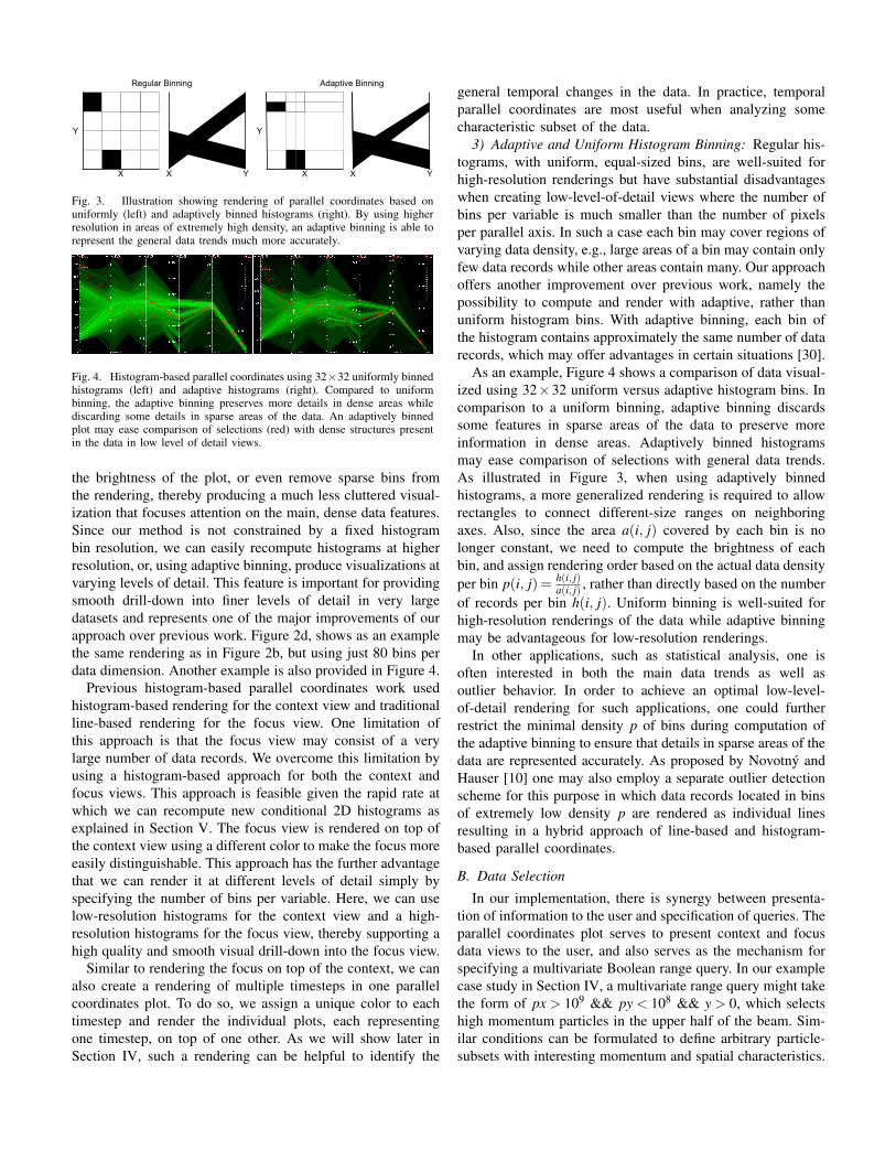
Fig. 3. Illustration showing rendering of parallel coordinates based onuniformly (left) and adaptively binned histograms (right). By using higherresolution in areas of extremely high density, an adaptive binning is able torepresent the general data trends much more accurately.

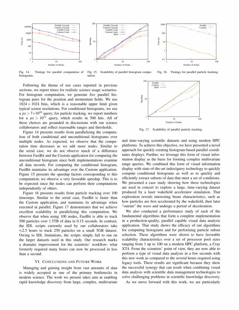
Fig. 4. Histogram-based parallel coordinates using 32×32 uniformly binnedhistograms (left) and adaptive histograms (right). Compared to uniformbinning, the adaptive binning preserves more details in dense areas whilediscarding some details in sparse areas of the data. An adaptively binnedplot may ease comparison of selections (red) with dense structures presentin the data in low level of detail views.

the brightness of the plot, or even remove sparse bins fromthe rendering, thereby producing a much less cluttered visual-ization that focuses attention on the main, dense data features.Since our method is not constrained by a fixed histogrambin resolution, we can easily recompute histograms at higherresolution, or, using adaptive binning, produce visualizations atvarying levels of detail. This feature is important for providingsmooth drill-down into finer levels of detail in very largedatasets and represents one of the major improvements of ourapproach over previous work. Figure 2d, shows as an examplethe same rendering as in Figure 2b, but using just 80 bins perdata dimension. Another example is also provided in Figure 4.

Previous histogram-based parallel coordinates work usedhistogram-based rendering for the context view and traditionalline-based rendering for the focus view. One limitation ofthis approach is that the focus view may consist of a verylarge number of data records. We overcome this limitation byusing a histogram-based approach for both the context andfocus views. This approach is feasible given the rapid rate atwhich we can recompute new conditional 2D histograms asexplained in Section V. The focus view is rendered on top ofthe context view using a different color to make the focus moreeasily distinguishable. This approach has the further advantagethat we can render it at different levels of detail simply byspecifying the number of bins per variable. Here, we can uselow-resolution histograms for the context view and a high-resolution histograms for the focus view, thereby supporting ahigh quality and smooth visual drill-down into the focus view.

Similar to rendering the focus on top of the context, we canalso create a rendering of multiple timesteps in one parallelcoordinates plot. To do so, we assign a unique color to eachtimestep and render the individual plots, each representingone timestep, on top of one other. As we will show later inSection IV, such a rendering can be helpful to identify the

general temporal changes in the data. In practice, temporalparallel coordinates are most useful when analyzing somecharacteristic subset of the data.

3) Adaptive and Uniform Histogram Binning: Regular his-tograms, with uniform, equal-sized bins, are well-suited forhigh-resolution renderings but have substantial disadvantageswhen creating low-level-of-detail views where the number ofbins per variable is much smaller than the number of pixelsper parallel axis. In such a case each bin may cover regions ofvarying data density, e.g., large areas of a bin may contain onlyfew data records while other areas contain many. Our approachoffers another improvement over previous work, namely thepossibility to compute and render with adaptive, rather thanuniform histogram bins. With adaptive binning, each bin ofthe histogram contains approximately the same number of datarecords, which may offer advantages in certain situations [30].

As an example, Figure 4 shows a comparison of data visual-ized using 32×32 uniform versus adaptive histogram bins. Incomparison to a uniform binning, adaptive binning discardssome features in sparse areas of the data to preserve moreinformation in dense areas. Adaptively binned histogramsmay ease comparison of selections with general data trends.As illustrated in Figure 3, when using adaptively binnedhistograms, a more generalized rendering is required to allowrectangles to connect different-size ranges on neighboringaxes. Also, since the area a(i, j) covered by each bin is nolonger constant, we need to compute the brightness of eachbin, and assign rendering order based on the actual data densityper bin p(i, j) = h(i, j)

a(i, j) , rather than directly based on the numberof records per bin h(i, j). Uniform binning is well-suited forhigh-resolution renderings of the data while adaptive binningmay be advantageous for low-resolution renderings.

In other applications, such as statistical analysis, one isoften interested in both the main data trends as well asoutlier behavior. In order to achieve an optimal low-level-of-detail rendering for such applications, one could furtherrestrict the minimal density p of bins during computation ofthe adaptive binning to ensure that details in sparse areas of thedata are represented accurately. As proposed by Novotny andHauser [10] one may also employ a separate outlier detectionscheme for this purpose in which data records located in binsof extremely low density p are rendered as individual linesresulting in a hybrid approach of line-based and histogram-based parallel coordinates.

B. Data Selection

In our implementation, there is synergy between presenta-tion of information to the user and specification of queries. Theparallel coordinates plot serves to present context and focusdata views to the user, and also serves as the mechanism forspecifying a multivariate Boolean range query. In our examplecase study in Section IV, a multivariate range query might takethe form of px > 109 && py < 108 && y > 0, which selectshigh momentum particles in the upper half of the beam. Sim-ilar conditions can be formulated to define arbitrary particle-subsets with interesting momentum and spatial characteristics.

Once the user specifies such a multivariate range condition,those conditions are passed back upstream in the system tothe FastBit-enhanced HDF5 reader for processing, either tocompute new histograms or to extract data subsets that matchthe query for downstream processing. In the case of datasubsetting, FastBit will locate those data records that satisfythe query and then pass them along for downstream process-ing. For conditional histograms, FastBit will compute newhistograms using the query conditions as well as a histogramspecification: the number of bins and the bin boundaries.

Once an interesting subset has been identified, yet anotherform of query can be issued in order to identify the same datasubset (here particles) at different points in time. This type ofquery is of the form ID IN (id1, id2, ..idn), where there are nparticles in the subset. Again, such queries can be processedefficiently by FastBit and only the relevant set of particlesis extracted and then passed along to visual data analysismachinery. This processing step offers a huge performanceadvantage: a technique without access to the index informationmust search the entire dataset for particle identifier matches.By issuing an identifier query across the entire time sequence,we construct particle tracks, which reveal valuable informationabout how particles are accelerated over time.

IV. USE CASE

We now present a specific example where we apply oursystem to perform visual data analysis of 2D and 3D dataproduced by a laser wakefield particle accelerator simulation.These simulations model the effects of a laser pulse propagat-ing through a hydrogen plasma. Similar to the wake of a boat,the radiation pressure of the laser pulse displaces the electronsin the plasma, and with the space-charge restoring force of theions, this displacement drives a wave (wake) in the plasma.Electrons can be trapped and accelerated by the longitudinalfield of the wake, forming electron bunches of high energy.Due to the large amount of particles required in order achieveaccurate simulation results, it is not possible to simulate theentire plasma at once. As a result, the simulation is restricted toa window that covers only a subset of the plasma in x directionin the vicinity of the beam. The simulation code moves thewindow along the local x axis over the course of the run.

The simulation data in these examples contains informationabout the position of particles in physical space –x, y, z –,particle momentum – px, py, pz – and particle ID at multipletimesteps. As a derived quantity, we also include the relativeparticle position in x direction within the simulation windowxrel(t) = x(t)−max(x(t)). There are more than 400,000 and90 million particles per timestep in the 2D and 3D datasets,respectively. The 2D data consists of 38 timesteps and has anoverall size of about 1.3GB, including the index structures.The 3D dataset consists of 30 timesteps and has an overallsize of about 210GB, including the index. Each 3D timestephas a size of about 7GB, including the index, and about 5GBwithout the index. We perform a detailed analysis of the 2Ddataset and then extend our analysis to the larger 3D dataset.

a) b)

d)px(x10^9)

py(x10^9)

pz(x10^9)

x(x10^-3)

y(x10^-6) id

Y-Axis (x10^-6)

X-Axis (x10^-6) 1270 1280 1310 1320 1290 1300

-30

-20

-10

0

10

20

30

c)

Y-Axis (x10^-6)

-30

-20

-10

0

10

20

30

X-Axis (x10^-6) 1750 1760 1790 1800 1770 1780

px(x10^9)

py(x10^9)

pz(x10^9)

x(x10^-3)

y(x10^-6) id

Fig. 5. a) Parallel coordinates and b) pseudocolor plot of the beam at t = 27.Corresponding plots c,d) at t = 37. The context plot, shown in red, shows bothbeams selected by the user after applying a threshold of px > 8.872 ∗ 1010

at t = 37. The focus plot, shown in green, indicates the first beam that isfollowing the laser pulse. In the pseudocolor plots b) and d), we show allparticles in gray and the selected beams using spheres colored according tothe particle’s x-momentum, px. The focus beam is the rightmost bunch inthese images. At timestep t = 27, the particles of the first beam (green infigure a) show much higher acceleration and a much lower energy spread(indicated via px) than the particles of the second beam. At later times, thelower momentum of the first beam indicates it has outrun the wave and movedinto decelerating phase, e.g at timestep t = 37.

In order to gain a deeper understanding of the accelerationprocess, we need to address complex questions such as: i)which particles become accelerated; ii) how are particlesaccelerated, and iii) how was the beam of highly acceleratedparticles formed and how did it evolve [31]. To identify thoseparticles that were accelerated, we first perform selection ofparticles at a late timestep (t = 37) of the simulation by usinga threshold for the value for x-momentum, px (Section IV-A).By tracing the selected particles over time we will then analyzethe behavior of the beam during late timesteps (Section IV-B).Having defined the beam, we can analyze formation andevolution of the beam by tracing particles further back to thetime where they entered the simulation and became injectedinto the beam (Section IV-C to IV-E). In this context, we useselection of particles, ID-based tracing of particles over time,and refinement of particle selections based on informationfrom different timesteps as main analysis techniques.

As we will illustrate in this use case, the ability to performselection interactively and immediately validate selectionsdirectly in parallel coordinates as well as other types ofplots, such as pseudocolor or scatter-plots, enables much moreaccurate selection than previously possible. Tracing of parti-cles over time then enables researchers to better understandevolution of the beam. With our visualization system the

t=14

t=15

t=16

t=17

X-Axis (x10^-6)

Y-Axis(x10^-6) 0

-10

-20

-30

30

20

10

660 680 700 720 760 780 800740 820

X-Axis (x10^-6)

Y-Axis(x10^-6) 0

-10

-20

-30

30

20

10

660 680 700 720 760 780 800740 820

X-Axis (x10^-6)

Y-Axis(x10^-6) 0

-10

-20

-30

30

20

10

660 680 700 720 760 780 800740 820

X-Axis (x10^-6)

Y-Axis(x10^-6) 0

-10

-20

-30

30

20

10

660 680 700 720 760 780 800740 820

Fig. 6. Particles of the beam at timestep 14 (top left) to 17 (bottom right).The color of selected particles indicates x-momentum, px, using a rainbowcolor map (red=high, blue=low). Non-selected particles are shown in gray.We can readily identify two main sets of particles entering the simulation attimestep t = 14 and additional sets of particles entering at t = 15.

1415

1617

X-Axis (x10^-6)660 680 700 720 740 760 780 800

Y-Axis (x10^-6)

-15

-10

-5

0

5

10

15

Fig. 7. The traces of the beam particles during timesteps t = 14 to t = 17as shown in Figure 6. The positions of the selected particles at the differenttimes are also shown. The begin and end of the timesteps in x direction areindicated below the bounding box. Here, we use color to indicate particle ID.

user can rapidly identify subsets of particles of interest andanalyze their temporal behavior. For “small” datasets one willusually perform all analysis on a regular workstation. Forlarger datasets VisIt can also be run in a distributed fashion sothat all heavy computation is performed on a remote machinewhere the data is stored and only the viewer and the GUI runon a local workstation.

A. Beam Selection

In order to identify the beam, i.e., find those particles thatbecame accelerated, we first concentrate on the last timestep of

1415

1617

a)

c)

px(x10^9)

py(x10^9)

pz(x10^9)

x(x10^-6)

y(x10^-6) id

X-Axis (x10^-6)

630 640 650 660 670 680

-30

-20

10

20

30b)

Y-Axis(x10^-6)

0

-10

X-Axis (x10^-6)X-Axis (x10^-6)660 680 700 720 740 760 780 800

-15

-10

-5

5

10

15

Y-Axis (x10^-6)

0

Fig. 8. a) By applying an additional threshold in x at timestep t = 14,we separate the two different set of particles entering the simulation. b) Therefinement result, shown in physical space, includes all non-selected particles(gray) to provide context. c) Particle traces of the complete beam and therefined selection. In all plots we show the complete beam in red and therefined selection in green. After entering the simulation, the selected particles(green) define first the outer part of the first beam at timestep t = 15. Lateron at timesteps t = 16 and t = 17, these particles become highly focused anddefine the center of the first beam.

t=14

t=15

t=16

t=17

t=18

t=19

t=20

t=21

t=22

Fig. 9. The beam at timesteps t = 14 to t = 22 in a temporal parallel coordi-nates plots. Here, color indicates each of the discrete timesteps. We can readilyidentify the two different beams in x and xrel (xrel(t) = x(t)−max(x(t))).While the second beam shows equal to higher values in px during earlytimesteps (t = 14 to t = 17), the first beam shows much higher accelerationat later times compared to the second beam.

the simulation (at t = 37). Using the parallel coordinates dis-play, we select the particles of interest by applying a thresholdof px > 8.872∗1010. As is visible in the parallel coordinatesplot, those particles constitute two separate clusters (beams)in x direction (Figure 5 c). Using a pseudocolor plot of thedata, we can then see the physical structure of the beam.

B. Beam Assessment

By tracing particles back in time, we observe that the firstbunch following the laser pulse (rightmost in these plots) haslower momentum spread at its peak energy (at t = 27) than thesecond bunch (see Figure 5a and 5b). In practice, the first beam

a) b)

px(x10^9)

x(x10^-6)

py(x10^9)

y(x10^-6)

pz(x10^9)

z(x10^-6) id

c)

Fig. 10. a) Parallel coordinates of timestep t = 12 of the 3D dataset. Context view (gray) shows particles selected with px > 2∗109. The focus view (red)shows particles satisfying the condition (px > 4.856∗1010) && (x > 5.649∗10−4), which form a compact beam in the first wake period following the laserpulse. b) Volume rendering of the plasma density and the selected focus particles (red). c) Traces of the beam. We selected particles at timestep t = 12, thentraced the particles back in time to timestep t = 9 when most of the selected particles entered the simulation window. We also traced the particles forward intime to timestep t = 14. Color indicates px. In addition to the traces and the position of the particles, we also show the context particles at timestep t = 12in gray to illustrate where the original selection was performed. We can see that the selected particles are constantly accelerated over time (increase in px).

following the laser pulse is therefore typically the one of mostinterest to the accelerator scientists. The fact that the secondbeam shows higher or equal acceleration at the last timestep ofthe simulation is due to the fact that the first beam will outrunthe wave later in time and therefore switches into a phase ofdeceleration while the second beam is still in an accelerationphase. In practice, when researchers want to select only thefirst beam, they usually perform selection of the particles usingthresholding in px at an earlier time (e.g. t = 27) when thebeam-particles of interest have maximum momentum, ratherthan the last timestep, here t = 37. By performing selectionat an earlier time, one avoids selecting particles in the secondbeam while being sure to select all particles in the first beam.In this specific use case we are interested in analyzing andcomparing the evolution of these two beams, which is whywe performed selection at the last timestep.

C. Beam Formation

Having defined the beam in the 2D dataset, we can analyzeformation of the beam by tracing the selected particles back tothe time when particles entered the simulation and were theninjected into the beam. In Figure 6, the individual particlesof the beam are shown at timesteps t = 14 to t = 17. Here,color indicates the particles’ momentum in the x direction(px). Figure 7 shows the particle traces over time coloredaccording to particle ID’s (the first beam appearing in blueand the second beam in yellow/red). Different sets of injectionare readily visible, and two sets of particles appear at t = 14.The left bunch will be injected to form a beam in the secondwake period, which is visible at t > 14. A second group ofparticles is just entering the right side of the box (recall thatthe simulation box is sweeping from left to right with the laser,so that plasma particles enter it from its right side). This bunchcontinues to enter at t = 15, and the particles stream into thefirst (rightmost) wake period. These particles are acceleratedand appear as a bunch in the first bucket for t > 15. At thefollowing timesteps t = 16 and t = 17, further acceleration ofthe two particle beams can be seen while only a few additional

particles are injected into the beam, and these are less focused,i.e., they show higher spread in the transverse direction (y).

D. Beam Refinement

Based on the information at timestep t = 14, we then refineour initial selection of the beam. By applying an additionalthreshold in x, we can select those particles of the beam thatare injected into the first wake period behind the laser pulse(see Figure 8a and 8b). By comparing the temporal traces ofthe selected particle subset (green) with the traces of the wholebeam (red), we can readily identify important characteristicsof the beam (see Figure 8c). After being injected, the selectedparticle subset (green) first defines the outer part of the firstbeam at timestep t = 15, while additional particles are injectedinto the center of the beam. Later on at timesteps t = 16and t = 17, the selected particles become strongly focusedand define the center of the first beam. By refining selectionsbased on information at an earlier time, we are able to identifycharacteristic substructures of the beam.

E. Beam Evolution

Using temporal parallel coordinates, we can analyze thegeneral evolution of the beam in multiple dimensions (seeFigure 9). Along the x axis, two separate beams can be seenat all timesteps (t = 14 to t = 22) with a quite stable relativeposition in x (xrel). At early timesteps, both beams showsimilar acceleration in px while later on, at timestep t = 18 tot = 22 (magenta to lilac), the particles of the first beam showsignificantly higher acceleration with a relatively low energyspread. We find particles at relatively high relative positionsin x direction (xrel) only at timesteps t = 14 and t = 15 dueto the fact that the particles of the beams enter the simulationwindow at these times.

F. 3D Analysis Example

We now describe a similar example analysis of the 3Dparticle dataset. Figure 10(a and b) shows the beam selectionstep for this dataset. At a much earlier timestep t = 12 (x ≈5.7∗10−4 compared to x≈ 1.3∗10−3 in the 2D case) particles

are trapped and accelerated. In order to get an overview ofthe main relevant data, the user removed the background fromthe data first by applying a threshold of px > 2.0 ∗ 109. Theuser then selected particles in the first bunch via thresholdingbased on the momentum in x direction (px > 4.586 ∗ 1010)and x position (x > 5.649 ∗ 10−4) to exclude particles in thesecondary periods from the selection. Figure 10b shows avolume rendering of the plasma density along with the selectedparticles revealing the physical location of the selected beamwithin the wake.

Figure 10c shows the traces of the particles selected earlierin Figure 10a. We selected the particles at timestep t = 12then traced them back to timestep t = 9 where most of theselected particles enter the simulation window and forward intime to timestep t = 14. As one can see in the plot, the selectedparticles are constantly accelerated over time.

V. PERFORMANCE EVALUATION

In this section, we present results of a study aimed at charac-terizing the performance of our implementation under varyingconditions using standalone, benchmark applications. Theseunit tests reflect the different stages of processing we presentedearlier in Section IV, the Use Case study. First, we examine theserial performance of histogram computation in Section V-A:histograms serve as the basis for visually presenting data to auser via a parallel coordinates plot. Second, in Section V-B, weexamine the serial performance of particle selection based onID across all time steps of simulation data. Finally in SectionV-C, we examine the parallel scalability characteristics of ourhistogram computation and particle tracking implementationson a Cray XT4 system.

For the serial performance tests in Sections V-A and V-B,we use the 3D dataset described earlier in Section IV: 30timesteps worth of accelerator simulation data, each timestephaving about 90 million particles and being ≈ 7GB in size(including ≈ 2GB for the index). The aggregate dataset size isabout 210GB, including the index data. We store and retrievesimulation and index data using HDF5 and a veneer librarycalled HDF5-FastQuery [32]. HDF5-FastQuery presents animplementation-neutral API for performing queries and ob-taining histograms of data. We conduct the serial performancetests on a workstation equipped with a 2.2GHz AMD OpteronCPU, 4GB of RAM and running the SuSE Linux distribution.

The serial performance tests in Sections V-A and V-Bmeasure the execution time of two different implementationsthat are standalone applications we created for the purposeof this performance experiment. One application, labeled“FastBit” in the charts, uses FastBit for index/query andhistogram computation. The other, labeled “Custom” in thecharts, does not use any indexing structure, and thereforeperforms a sequential scan of the dataset when computinghistograms and particle selections. Note, in order to enablea fair comparison we here use our own Custom code whichshows better performance than the IDL scripts currently usedby our science collaborators.

A. Computing 2D HistogramsWe run a pair of test batteries aimed at differentiating

performance characteristics of computing both unconditionaland conditional histograms. The unconditional histogram issimply a histogram of an entire dataset using a set ofapplication-defined bin boundaries. A conditional histogramis one computed from a subset of data records that match anexternal condition.

1) Unconditional Histograms: In our use model, the com-putation of the unconditional histogram is a “one-time” oper-ation. It provides the initial context view of a dataset.

For this test, we vary the number of bins in a 2D histogramover the following bin resolutions: 32×32, 64×64, 128×128,256×256, 512×512, 1024×1024, and 2048×2048 bins. Allhistograms span the same range of data values: increasing thebin count results in bins of finer resolution. The results of thistest are shown in Figure 11. Since both the FastBit and Customapplications need to examine all the data records to compute anunconditional histogram, we do not expect much performancevariation as we change the number of bins. FastBit is generallyfaster than the custom code throughout primarily because ofthe difference in organization of the histogram bin countsarray. FastBit uses a single array, which results in a morefavorable memory access pattern. FastBit computes adaptivehistograms by first computing a higher-resolution uniformlybinned histogram and then merging bins. Since merging binsis a fairly inexpensive process and increasing the number ofbins has no significant effect on the performance of uniformlybinned histograms we observe only a minor, constant increasein computation time for adaptive versus uniform binning.

2) Conditional Histograms: In contrast to the unconditionalhistogram, which is a one-time computation, the process ofvisual data exploration and mining relies on repeated computa-tions of conditional histograms. Therefore, we are particularlyinterested in achieving good performance of this operationto support interactive visual data analysis. This set of testsfocuses on a use model, a change in the set of conditionsresults in examining a greater or lesser number of data recordsto compute a conditional histogram. This set of conditionsreflects the repeated refinement associated with interactive,visual data analysis.

We parameterize our test based on the number of hitsresulting from a range of different queries. We use thresholdsof the form px > ... as the histogram conditions. As weincrease the threshold of particle momentum in the x directionwith this condition, fewer data records (particles) satisfy thatcondition and contribute to the resulting histogram. In thesetests, we hold the number of bins constant at 1024×1024.

Figure 12 presents results for computing conditional his-tograms using FastBit and the Custom application. We observethat for small number of hits, the FastBit execution times aredramatically faster than the Custom code that examines alldata records. Also, in this regime we observe that uniformand adaptive binning show similar performance. While forunconditional histograms the minimum and maximum valuesare known for each variable, we here need to compute these

0

1

2

3

4

5

6

7

8

1000 10000 100000 1e+06 1e+07

Tim

e (s

)

Number of Bins

FastBit-RegularFastBit-AdaptiveCustom-Regular

Fig. 11. Timings for serial computation of uncon-ditional histograms.

0

1

2

3

4

5

6

7

8

10 100 1000 10000 100000 1e+06 1e+07 1e+08

Tim

e (s

)

Number of Hits

FastBit-RegularFastBit-AdaptiveCustom-Regular

Fig. 12. Timings for serial computation of con-ditional histograms.

1e-04

0.001

0.01

0.1

1

10

100

10 100 1000 10000 100000 1e+06 1e+07 1e+08

Tim

e (s

)

Number of Hits

FastBitCustom

Fig. 13. Timings for serial processing of identifierqueries.

values from the selected data parts in order to compute theadaptive binning. Due to this fact we observe a performance-decrease of the adaptive binning compared to uniform binningfor very large selections. It is important to note that visualanalysis queries typically isolate a small number of particles– from tens to thousands – and FastBit provides outstandingperformance in this regime. As the number of hits increases,approaching 1M and 10M+ particles – which is a significantfraction of the 90M total particles – a sequential scan throughall the data records produces better results. This performancechange is due to the fact that FastBit computes the histogramin two separate steps. It first evaluates the user-specifiedconditions to select the appropriate values, and then counts thenumber of values in each histogram-bin. The selected valuesare passed from the first to the second step as an intermediatearray with as many elements as the number of hits. It isexpensive to pass this intermediate array through memorywhen it is large. Since the intended applications primarily havea small number of hits, using FastBit is more efficient.

B. Particle Selections

Following our use model, once a user has determineda set of interesting data conditions, like particles having amomentum exceeding a given threshold, the next activity isto extract those particles from the large dataset for subsequentanalysis. This set of tests aims to show performance of theparticle subsetting part of the processing pipeline.

The execution time for this task is clearly proportional tothe size of the selection – the time required to find a set ofparticles in a large, time-varying dataset varies as a functionof the size of the particle search set as well as the size of thesimulation data itself. We parameterize the search set size forthis set of performance tests, varying the number of particlesto search for over values ranging from 10, 100, 1000, ... , upto 20M particles.

Our custom code uses a sequential scan of the entire datasetto search for particles in the search set. For each data record,it compares the particle ID of the record to the search setusing an efficient algorithm: if the size of the search set isS, then the search time is O(log(S)). If there are N datarecords in the entire dataset, the computational complexity ofthe entire algorithm is O(Nlog(S)). In contrast, the worst-case

time required to locate a set of identifiers using FastBit isexpected to be proportional to the number records found [17].

Figure 13 presents results for running ID queries usingFastBit and the Custom code for one timestep. For relativelysmall numbers of identifiers, we observe that FastBit is aboutfour orders of magnitude (104×) faster than the Custom code.As the number of identifiers involved increases, the relativedifference becomes smaller. When 20 million of identifies areinvolved, FastBit is still three times faster.

C. Scalability Tests

Whereas the previous sections have focused on the serialperformance of computing histograms and performing parti-cle subset selections, this section focuses on the scalabilitycharacteristics of both algorithms.

The platform for these tests is franklin.nersc.gov,a 9,660 node, 19K core Cray XT4 system. Each of the nodesconsists of a 2.6GHz, dual-core AMD Opteron processor andhas 4GB of memory and runs the Compute Node Linuxdistribution. One optimization we use on this machine at alllevels of parallelism is to restrict operations to a single coreof each node. This optimization maximizes the amount ofmemory and I/O bandwidth available to each process in ourparallel performance tests. On this platform, the Lustre ParallelFilesystem serves data to each of the nodes. The nodes used inthe study are a small fraction of a larger shared facility witha dynamic workload. Our scalability tests cover parallelismlevels over the following range: 1, 2, 5, 10, 20, 50, and 100nodes of the Cray XT4.

As in previous sections, we report wall-clock times whichencapsulate CPU processing and I/O. We report the speedupfactor as the ratio of time taken by a single node to the timetaken by the node subset to complete a task. We do a strongscaling test by keeping the problem size fixed at 100 timestepsfor all cases.

The dataset used in this study has 100 timesteps; eachtimestep has 177 million particles and is about 10GB in size.The aggregate dataset size is about 1.5T B, including the indexdata. We employ a fairly simple form of data partitioning forthese scalability tests: namely we assign data subsets corre-sponding to individual timesteps (corresponding to individualHDF5 files) to individual nodes for processing. The subsetsare statically assigned to nodes in a strided fashion.

1

10

100

1000

10000

100000

1 10 100

Tim

e (s

)

Number of Nodes

FastBit Uncond.Custom Uncond.

FastBit Cond.Custom Cond.

Fig. 14. Timings for parallel computation ofhistograms.

1

10

100

1 10 100

Spee

dup

Number of Nodes

FastBit Uncond.Custom Uncond.

FastBit Cond.Custom Cond.

Ideal

Fig. 15. Scalability of parallel histogram compu-tation.

0.1

1

10

100

1000

1 10 100

Tim

e (s

)

Number of Nodes

FastBitCustom

Fig. 16. Timings for parallel particle tracking.

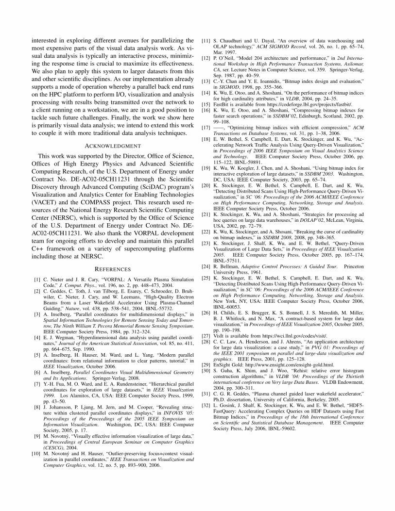
Following the theme of use cases reported in previoussections, we report times for realistic science usage scenarios.For histogram computation, we generate five parallel his-togram pairs for the position and momentum fields. We use1024× 1024 bins, which is a reasonable upper limit giventypical screen resolutions. For conditional histograms, we usea px > 7∗1010 query; for particle tracking, we report numbersfor a px > 1011 query, which results in 500 hits. All ofthese choices are grounded in discussions with our sciencecollaborators and reflect reasonable ranges and thresholds.

Figure 14 presents results from parallelizing the computa-tion of both conditional and unconditional histograms overmultiple nodes. As expected, we observe that the compu-tation time decreases as we add more nodes. Similar tothe serial case, we do not observe much of a differencebetween FastBit and the Custom application for computing theunconditional histogram since both implementations examineall data records. For computing the conditional histogram,FastBit maintains its advantage over the Custom application.Figure 15 presents the speedup factors corresponding to thiscomputation; we observe a very favorable speedup. This is tobe expected since the nodes can perform their computationsindependently of others.

Figure 16 presents results from particle tracking over 100timesteps. Similar to the serial case, FastBit is faster thanthe Custom application, and maintains its advantage whenexecuted in parallel. Figure 17 demonstrates that we achieveexcellent scalability in parallelizing this computation. Weobserve that when using 100 nodes, FastBit is able to track500 particles over 1.5TB of data in 0.15 seconds. In contrast,the IDL scripts currently used by our collaborators take≈2.5 hours to track 250 particles on a small 5GB dataset.Owing to IDL limitations, the scripts simply fail to run onthe larger datasets used in this study. Our research marksa dramatic improvement for the scientists’ workflow: whatformerly required many hours can now be processed in lessthan a second.

VI. CONCLUSIONS AND FUTURE WORK

Managing and gaining insight from vast amounts of datais widely accepted as one of the primary bottlenecks inmodern science. The work we present takes aim at enablingrapid knowledge discovery from large, complex, multivariate

1

10

100

1 10 100

Spee

dup

Number of Nodes

FastBitCustom

Ideal

Fig. 17. Scalability of parallel particle tracking.

and time-varying scientific datasets and using modern HPCplatforms. To achieve this objective, we have presented a novelapproach for quickly creating histogram-based parallel coordi-nates displays. Further, we leverage this form of visual infor-mation display as the basis for forming complex multivariaterange queries. We combined this form of visual informationdisplay with state-of-the-art index/query technology to quicklycompute conditional histograms as well as to quickly andefficiently extract subsets of data that meet a set of conditions.We presented a case study showing how these technologiesare used in concert to explore a large, time-varying datasetproduced by a laser wakefield accelerator simulation. Thatexploration reveals interesting beam characteristics, such ashow particles are first accelerated by the wakefield, then later“outrun” the wave and undergo a period of deceleration.

We also conducted a performance study of each of thefundamental algorithms that form a complete implementationin a production-quality, parallel capable visual data analysisapplication. That study shows the efficacy of our algorithmsfor computing histograms and for performing particle subsetselection. These algorithms were shown to have favorablescalability characteristics over a set of processor pool sizesranging from 1 up to 100 on a modern HPC platform, a CrayXT4. From the scientists’ point of view, they are now able toperform a type of visual data analysis in a few seconds withthis new work as compared to the several hours required usinglegacy tools. These results are significant because they showthe successful synergy that can result when combining visualdata analysis with scientific data management technologies tosolve challenging problems in scientific knowledge discovery.

As we move forward with this work, we are particularly

interested in exploring different avenues for parallelizing themost expensive parts of the visual data analysis work. As vi-sual data analysis is typically an interactive process, minimiz-ing the response time is crucial to maximize its effectiveness.We also plan to apply this system to larger datasets from thisand other scientific disciplines. As our implementation alreadysupports a mode of operation whereby a parallel back end runson the HPC platform to perform I/O, visualization and analysisprocessing with results being transmitted over the network toa client running on a workstation, we are in a good position totackle such future challenges. Finally, the work we show hereis primarily visual data analysis; we intend to extend this workto couple it with more traditional data analysis techniques.

ACKNOWLEDGMENT

This work was supported by the Director, Office of Science,Offices of High Energy Physics and Advanced ScientificComputing Research, of the U.S. Department of Energy underContract No. DE-AC02-05CH11231 through the ScientificDiscovery through Advanced Computing (SciDAC) program’sVisualization and Analytics Center for Enabling Technologies(VACET) and the COMPASS project. This research used re-sources of the National Energy Research Scientific ComputingCenter (NERSC), which is supported by the Office of Scienceof the U.S. Department of Energy under Contract No. DE-AC02-05CH11231. We also thank the VORPAL developmentteam for ongoing efforts to develop and maintain this parallelC++ framework on a variety of supercomputing platformsincluding those at NERSC.

REFERENCES

[1] C. Nieter and J. R. Cary, “VORPAL: A Versatile Plasma SimulationCode,” J. Comput. Phys., vol. 196, no. 2, pp. 448–473, 2004.

[2] C. Geddes, C. Toth, J. van Tilborg, E. Esarey, C. Schroeder, D. Bruh-wiler, C. Nieter, J. Cary, and W. Leemans, “High-Quality ElectronBeams from a Laser Wakefield Accelerator Using Plasma-ChannelGuiding,” Nature, vol. 438, pp. 538–541, 2004, lBNL-55732.

[3] A. Inselberg, “Parallel coordinates for multidimensional displays,” inSpatial Information Technologies for Remote Sensing Today and Tomor-row, The Ninth William T. Pecora Memorial Remote Sensing Symposium.IEEE Computer Society Press, 1984, pp. 312–324.

[4] E. J. Wegman, “Hyperdimensional data analysis using parallel coordi-nates,” Journal of the American Statistical Association, vol. 85, no. 411,pp. 664–675, Sep. 1990.

[5] A. Inselberg, H. Hauser, M. Ward, and L. Yang, “Modern parallelcoordinates: from relational information to clear patterns, tutorial,” inIEEE Visualization, October 2006.

[6] A. Inselberg, Parallel Coordinates Visual Multidimensional Geometryand Its Applications. Springer-Verlag, 2008.

[7] Y.-H. Fua, M. O. Ward, and E. A. Rundensteiner, “Hierarchical parallelcoordinates for exploration of large datasets,” in IEEE Visualization1999. Los Alamitos, CA, USA: IEEE Computer Society Press, 1999,pp. 43–50.

[8] J. Johansson, P. Ljung, M. Jern, and M. Cooper, “Revealing struc-ture within clustered parallel coordinates displays,” in INFOVIS ’05:Proceedings of the Proceedings of the 2005 IEEE Symposium onInformation Visualization. Washington, DC, USA: IEEE ComputerSociety, 2005, p. 17.

[9] M. Novotny, “Visually effective information visualization of large data,”in Proceedings of Central European Seminar on Computer Graphics(CESCG), 2004.

[10] M. Novotny and H. Hauser, “Outlier-preserving focus+context visual-ization in parallel coordinates,” IEEE Transactions on Visualization andComputer Graphics, vol. 12, no. 5, pp. 893–900, 2006.

[11] S. Chaudhuri and U. Dayal, “An overview of data warehousing andOLAP technology,” ACM SIGMOD Record, vol. 26, no. 1, pp. 65–74,Mar. 1997.

[12] P. O’Neil, “Model 204 architecture and performance,” in 2nd Interna-tional Workshop in High Performance Transaction Systems, Asilomar,CA, ser. Lecture Notes in Computer Science, vol. 359. Springer-Verlag,Sep. 1987, pp. 40–59.

[13] C.-Y. Chan and Y. E. Ioannidis, “Bitmap index design and evaluation,”in SIGMOD, 1998, pp. 355–366.

[14] K. Wu, E. Otoo, and A. Shoshani, “On the performance of bitmap indicesfor high cardinality attributes,” in VLDB, 2004, pp. 24–35.

[15] FastBit is available from https://codeforge.lbl.gov/projects/fastbit/.[16] K. Wu, E. Otoo, and A. Shoshani, “Compressing bitmap indexes for

faster search operations,” in SSDBM’02, Edinburgh, Scotland, 2002, pp.99–108.

[17] ——, “Optimizing bitmap indices with efficient compression,” ACMTransactions on Database Systems, vol. 31, pp. 1–38, 2006.

[18] E. W. Bethel, S. Campbell, E. Dart, K. Stockinger, and K. Wu, “Ac-celerating Network Traffic Analysis Using Query-Driven Visualization,”in Proceedings of 2006 IEEE Symposium on Visual Analytics Scienceand Technology. IEEE Computer Society Press, October 2006, pp.115–122, lBNL-59891.

[19] K. Wu, W. Koegler, J. Chen, and A. Shoshani, “Using bitmap index forinteractive exploration of large datasets,” in SSDBM’2003. Washington,DC, USA: IEEE Computer Society, 2003, pp. 65–74.

[20] K. Stockinger, E. W. Bethel, S. Campbell, E. Dart, and K. Wu,“Detecting Distributed Scans Using High-Performance Query-Driven Vi-sualization,” in SC ’06: Proceedings of the 2006 ACM/IEEE Conferenceon High Performance Computing, Networking, Storage and Analysis.IEEE Computer Society Press, October 2006.

[21] K. Stockinger, K. Wu, and A. Shoshani, “Strategies for processing adhoc queries on large data warehouses,” in DOLAP’02, McLean, Virginia,USA, 2002, pp. 72–79.

[22] K. Wu, K. Stockinger, and A. Shosani, “Breaking the curse of cardinalityon bitmap indexes,” in SSDBM 2008, 2008, pp. 348–365.

[23] K. Stockinger, J. Shalf, K. Wu, and E. W. Bethel, “Query-DrivenVisualization of Large Data Sets,” in Proceedings of IEEE Visualization2005. IEEE Computer Society Press, October 2005, pp. 167–174,lBNL-57511.

[24] R. Bellman, Adaptive Control Processes: A Guided Tour. PrincetonUniversity Press, 1961.

[25] K. Stockinger, E. W. Bethel, S. Campbell, E. Dart, and K. Wu,“Detecting Distributed Scans Using High-Performance Query-Driven Vi-sualization,” in SC ’06: Proceedings of the 2006 ACM/IEEE Conferenceon High Performance Computing, Networking, Storage and Analysis.New York, NY, USA: IEEE Computer Society Press, October 2006,lBNL-60053.

[26] H. Childs, E. S. Brugger, K. S. Bonnell, J. S. Meredith, M. Miller,B. J. Whitlock, and N. Max, “A contract-based system for large datavisualization,” in Proceedings of IEEE Visualization 2005, October 2005,pp. 190–198.

[27] VisIt is available from https://wci.llnl.gov/codes/visit/.[28] C. C. Law, A. Henderson, and J. Ahrens, “An application architecture

for large data visualization: a case study,” in PVG 01: Proceedings ofthe IEEE 2001 symposium on parallel and large-data visualization andgraphics. IEEE Press, 2001, pp. 125–128.

[29] EnSight Gold: http://www.ensight.com/ensight-gold.html.[30] S. Guha, K. Shim, and J. Woo, “Rehist: relative error histogram

construction algorithms,” in VLDB ’04: Proceedings of the Thirtiethinternational conference on Very large Data Bases. VLDB Endowment,2004, pp. 300–311.

[31] C. G. R. Geddes, “Plasma channel guided laser wakefield accelerator,”Ph.D. dissertation, University of California, Berkeley, 2005.

[32] L. Gosink, J. Shalf, K. Stockinger, K. Wu, and E. W. Bethel, “HDF5-FastQuery: Accelerating Complex Queries on HDF Datasets using FastBitmap Indices,” in Proceedings of the 18th International Conferenceon Scientific and Statistical Database Management. IEEE ComputerSociety Press, July 2006, lBNL-59602.