UNLV Theses, Dissertations, Professional Papers, and Capstones

5-1-2016

High-Pressure Properties of Several Narrow Bandgap High-Pressure Properties of Several Narrow Bandgap

Semiconductors from First-Principles Calculations Semiconductors from First-Principles Calculations

Andrew Michael Alvarado University of Nevada, Las Vegas

Follow this and additional works at: https://digitalscholarship.unlv.edu/thesesdissertations

Part of the Condensed Matter Physics Commons, Engineering Science and Materials Commons, and

the Materials Science and Engineering Commons

Repository Citation Repository Citation Alvarado, Andrew Michael, "High-Pressure Properties of Several Narrow Bandgap Semiconductors from First-Principles Calculations" (2016). UNLV Theses, Dissertations, Professional Papers, and Capstones. 2629. http://dx.doi.org/10.34917/9112019

This Thesis is protected by copyright and/or related rights. It has been brought to you by Digital Scholarship@UNLV with permission from the rights-holder(s). You are free to use this Thesis in any way that is permitted by the copyright and related rights legislation that applies to your use. For other uses you need to obtain permission from the rights-holder(s) directly, unless additional rights are indicated by a Creative Commons license in the record and/or on the work itself. This Thesis has been accepted for inclusion in UNLV Theses, Dissertations, Professional Papers, and Capstones by an authorized administrator of Digital Scholarship@UNLV. For more information, please contact digitalscholarship@unlv.edu.

HIGH-PRESSURE PROPERTIES OF SEVERAL NARROW BANDGAP

SEMICONDUCTORS FROM FIRST-PRINCIPLES CALCULATIONS

By

Andrew M. Alvarado

Bachelor of Science – Physics

University of Nevada, Las Vegas

2014

A thesis submitted in partial fulfillment

of the requirements for the

Master of Science – Physics

Department of Physics and Astronomy

College of Sciences

The Graduate College

University of Nevada, Las Vegas

May 2016

ii

Thesis Approval

The Graduate College

The University of Nevada, Las Vegas

April 4, 2016

This thesis prepared by

Andrew M. Alvarado

entitled

High-Pressure Properties of Several Narrow Bandgap

Semiconductors from First-Principles Calculations

is approved in partial fulfillment of the requirements for the degree of

Master of Science – Physics

Department of Physics and Astronomy

Changfeng Chen, Ph.D. Kathryn Hausbeck Korgan, Ph.D. Examination Committee Chair Graduate College Interim Dean

Andrew L. Cornelius, Ph.D. Examination Committee Member

Ravhi S. Kumar, Ph.D. Examination Committee Member

Pamela Burnley, Ph.D. Graduate College Faculty Representative

iii

ABSTRACT

High-pressure Properties of Several Narrow Bandgap Semiconductors from First-Principles

Calculations

By

Andrew Alvarado

Dr. Changfeng Chen, Examination Committee Chair

Professor of Physics

University of Nevada, Las Vegas

The electronic, thermodynamic, and structural properties of three semiconducting materials,

ZnO, InN, and PbS, at high pressure are investigated utilizing first-principles calculations based

on density function theory. The first two systems, ZnO and InN, crystalize as hexagonal

structures at ambient conditions and transition to a cubic structure at higher pressures. The last

system, PbS, is cubic at ambient conditions, but transitions to an orthorhombic structure at higher

pressure. At ambient conditions, these materials are well known semiconductors with vast

amount of research and a variety of wide ranging applications in electrical devices. However,

there is a lack of understanding of their physical properties at high pressures. In this thesis, an

attempt is made to establish an understanding of the fundamental properties of the high-pressure

phase of these materials. DFT and Boltzmann transport theory are used to find how pressure-

induced phase transitions affect the electronic and heat transport of these materials. From

harmonic approximations, a frozen phonon method is used to calculate the phonon frequencies

and thermodynamic properties.

iv

ACKNOWLEDGEMENTS

I would like to thank and express my deepest gratitude to Dr. Changfeng Chen for being my

advisor and mentor. Dr. Chen has taught me more than I can receive from any classroom. As a

freshman with little knowledge in physics, Dr. Chen allowed me to join his research group. Dr.

Chen has given me task and projects to prepare me for classes and onward. I sincerely appreciate

Dr. Chen and all he has done for me. From statistical mechanics to the ethics of working in and

out of a research group, Dr. Chen has taught valuable lessons of life in general.

I also thank Dr. Yi Zhang who has taught me how to use a number of computational programs

and explaining to me the physics behind them. I also appreciate the discussions and meetings we

had to go over my research and his patience in working with me.

I would also like to thank Jeevake Attapattu, Christopher Higgins, and William Wolfs. As fellow

students, they supported and studied with me.

Finally, I would like to thank my family and friends for all their support.

v

TABLE OF CONTENTS

ABSTRACT ............................................................................................................................... iii

ACKNOWLEDGEMENT ......................................................................................................... iv

LIST OF TABLES ..................................................................................................................... vi

LIST OF FIGURES ................................................................................................................... vii

CHAPTER 1: INTRODUCTION ............................................................................................. 1

CHAPTER 2: BACKGROUND AND THEORY ....................................................................... 3

CRYSTAL STRUCTURE ................................................................................................ 3

N-BODY SCHRODINGER EQUATION ........................................................................ 7

DENSITY FUNCTIONAL THEORY ............................................................................ 11

ELECTRONIC TRANSPORT THEORY ...................................................................... 22

LATTICE DYNAMICS .................................................................................................. 29

CHAPTER 3: THERMOELECTRIC PROPERTIES OF ROCKSALT ZnO ............................ 35

CHAPTER 4: HIGH-PRESSURE PROPERTIES OF ROCKSALT InN .................................. 53

CHAPTER 5: PHASE-TRANSITION INDUCED GAP TRANSITION IN PbS ..................... 71

REFERENCES ........................................................................................................................... 79

CURRICULUM VITAE ............................................................................................................. 87

vi

LIST OF TABLES

TABLE 2.1 List of Crystal Systems ............................................................................................ 5

vii

LIST OF FIGURES

Figure 2.1 Simple Cubic structure ................................................................................................ 4

Figure 2.2 Body-Centered Cubic structure ................................................................................... 5

Figure 2.3 Face-Centered Cubic structure .................................................................................... 5

Figure 3.1 Enthalpy versus Pressure curve for ZnO ................................................................... 39

Figure 3.2 Phonon Dispersion of RS ZnO at 0 and 20 GPa ....................................................... 41

Figure 3.3 Thermodynamic properties of RS and WZ ZnO ....................................................... 43

Figure 3.4 Thermal Conductivity of RS ZnO and experimental WZ ZnO ................................. 45

Figure 3.5 Electronic Band Structure of RS ZnO ....................................................................... 46

Figure 3.6 Transport Properties of n-type concentration of RS ZnO at 0 and 20 GPa ............... 48

Figure 3.7 Transport Properties of p-type concentration of RS ZnO at 0 and 20 GPa ............... 49

Figure 3.8 Figure of Merit ZT of RS ZnO at 0 and 20 GPa ....................................................... 51

Figure 4.1 Enthalpy versus Pressure curve for InN .................................................................... 56

Figure 4.2 Electronic Band Structure of RS InN at 0 and 13 GPa .............................................. 57

Figure 4.3 Electronic Band Structure of WZ InN at 0 GPa ........................................................ 59

Figure 4.4 Phonon Dispersion curve for RS InN at 0 and 13 GPa ............................................. 60

Figure 4.5 Phonon Dispersion curve for WZ InN at 0 GPa ........................................................ 61

Figure 4.6 Thermodynamic Properties of RS and WZ InN ........................................................ 63

Figure 4.7 Transport Properties of n-type and p-type concentration of RS InN at 0 GPa .......... 65

Figure 4.8 Transport Properties of n-type and p-type concentration of RS InN at 13 GPa ........ 66

Figure 4.9 Nudged Elastic Band plot of WZ to RS InN transition ............................................. 69

Figure 5.1 Enthalpy versus Pressure of varies phases of PbS ..................................................... 75

Figure 5.2 Volume versus Pressure of various phases of PbS .................................................... 76

viii

Figure 5.3 Electronic Band Structure of orthorhombic and cubic PbS ....................................... 77

1

CHAPTER 1

INTRODUCTION

Semiconductors are used in nearly every electrical device in today’s world. There are many

important semiconductors that are used in a variety of electrical devices. Silicon is one of the

world’s most highly produced semiconductors. Silicon is seen from integrated circuit boards to

solar panels. Like many other semiconductors, silicon has a variety of crystal structures at higher

pressures, each with their own interesting physical properties. However, studies on

semiconductors are done at or near ambient conditions due to experimental limitations. In this

thesis ZnO, InN, and PbS are investigated because, like silicon, they are well understood in their

ambient condition, but their behavior changes when they are introduced to pressure. A material

that is a semiconductor at ambient condition may become metallic or an insulator when the

pressure is increased. The band gap may either widen or become narrower. This can be due to a

pressure-induced phase transition.

In the second, the theory and background behind much of the calculations for each material are

discussed. The crystal structure of a material, density functional theory, and Boltzmann transport

theory are examined to develop means of calculating physical properties. Understanding the

crystal structure at various pressures of a material can help expand the knowledge of a material

phase diagram. Density functional theory transforms the many-bodied Schrödinger equation to a

single electron charge density dependent equation. Boltzmann transport theory and the

Boltzmann equation provide the capability to determine interesting transport properties. Finally,

software packages that implement the theory are introduced.

2

ZnO and InN both crystalize as a hexagonal wurtzite crystal structure in ambient conditions. It is

experimentally shown that they transition to a cubic rocksalt structure at higher pressures. [1, 2]

It is also shown that it is possible to stabilize their high-pressure structures much lower than their

transition pressures through epitaxial stabilization. [3, 4] In the third and fourth chapter of this

thesis, ZnO and InN, respectively, are investigated to compare their electrical and heat transport

between their respected ambient and high-pressure phases both above and below the pressure

transition. In addition to modeling their transport properties, calculations of the figure of merit

ZT were performed to surmise the potential of these materials as thermoelectrics.

In the fifth chapter an investigation in corroboration with experimentalists was made to find and

characterize the intermediate structure of PbS. PbS is a narrow band gap semiconductor that

belongs to a family of lead chalcogenides (PbS). This family is a sodium chloride structure in

ambient conditions and transitions to a caesium chloride structure at higher pressures. However,

PbS is shown to transition to an intermediate orthorhombic structure and then further to a

caesium chloride structure. [5] Here, two plausible orthorhombic structures are investigated to

see which of the two is more energetically stable, and then characterize its electronic and

structural properties.

3

CHAPTER 2

BACKGROUND AND THEORY

In this chapter, the crystal structure, density functional theory, Boltzmann transport theory, and

general phonon theory are discussed to provide the theory behind the study. The first section

entitled crystal structure discusses the basic concept behind defining crystalline features in

materials. The second section depicts the theory and functions used in general density functional

theory (DFT) to provide relaxed structure and ground state energy of n-electron systems. The

third section provides the theory behind transport properties of solid materials. The last section

gives the general theory behind calculating phonon frequencies through the frozen phonon

method.

CRYSTAL STRUCTURE

It is essential to discuss the theory behind the crystal structure of any solid material especially

since in this thesis a comparison between two different crystal structures at varying pressures is

made. A crystal structure, or Bravais lattice, is defined as the spacing and periodic arrangement

between units. Units can be the atoms, groups, or molecules in a system, but as long as there is a

periodic array it belongs to a lattice system and can be categorized under a Bravais lattice. For

solid materials and this study, atoms are the units. A unit cell can then be defined as a structure

of atoms in which are repeated throughout the solid. A vector that relates all the points in a

lattice is called the position vector. A general example of the position vector is:

!R = n1

!a1 + n2!a2 + n3

!a3

4

Where ni are integers and a1 are primitive vectors that generate the lattice. It must be noted that

for any Bravais lattice the primitive vectors are not unique. In fact, there are infinitely many

nonequivalent choices for the primitive vectors.

Although in ambient conditions semiconductors and metals can be in many different crystal

structures, in high-pressure they often transition into crystal structures with higher symmetry. [6]

A well-known and highly symmetric lattice is that of the cubic. The cubic lattice contains three

Bravais lattices: Simple cubic, body-centered cubic, and face-centered cubic. The simple cubic

structure can be described by three mutually orthogonal primitive vectors a1, a2, and a3 with

atoms at each corner of a unit cell.

Figure 2.1 The simple (primitive) cubic cell.

With primitive vectors

!a1 = ax, !a2 = ay,

!a3 = az.

The body-centered cubic structure contains an atom in the middle of a cell and atoms at each

corner of the cell.

→a3

→a1

→a2

5

Figure 2.2 The body-centered cubic cell.

With primitive vectors

!a1 = ax, !a2 = ay,

!a3 =a2(x + y+ z).

The face-centered cubic structure contains atoms at the center of each face of the cube as well as

every corner of the cell.

Figure 2.3 The face-centered cubic cell.

With primitive vectors

→a3

→a1

→a2

→a3

→a1→a2

6

!a1 =a2(y+ z),

!a2 =a2(z + x),

!a3 =a2(x + y).

There are 7 types of crystal systems and 14 Bravais lattice. Table 1.1 describes systems and their

associated number of lattice, along with restrictions on the vector length and the angle between

the primitive vectors. [7]

System Number of lattice Restrictions

Triclinic 1 a1≠a2≠a3, α ≠β ≠γ

Monoclinic 2 a1≠a2≠a3, α =γ =90o≠β

Orthorhombic 4 a1≠a2≠a3, α =β =γ =90o

Tetragonal 2 a1=a2≠a3, α =β =γ =90o

Cubic 3 a1=a2=a3, α =β =γ =90o

Trigonal 1 a1=a2=a3, α =β =γ < 120o

Hexagonal 1 a1=a2≠a3, α =β =90 , γ = 120o

Table 1.1 Crystal systems, their number of lattices, and restrictions. [7]

The figures depicted above are for single element materials. Here, binary compounds are

investigated. With cells containing two ions the Bravais lattice loses a translational symmetry. In

other words, all points do not look the same; instead there is some kind of interchanging of

atoms. For example the sodium chloride structure contains equal atoms at every Bravais lattice

point, but the corners of a cell alternate between sodium and chlorine ions. This type of structure

is that of a face-centered cubic Bravais lattice. The sodium chloride structure is also referred to

as the rock-salt structure.

7

N-BODY SCHRÖDINGER EQUATION

The many-body Schrödinger equation can used to study solid-state properties. First a

Hamiltonian that contains the kinetic energy and interactions of all the particles in a solid must

be defined. Within a solid there are the ions and the electrons, these ions and electrons can

interact with each other. Furthermore, the electrons can be distinguished between the valence

electrons and the core electrons. These valence electrons are the main drivers of interactions such

as chemical bonding. The cores electrons are usually strongly bound with the ions and do not

significantly contribute to material properties. Therefore the Hamiltonian can be simply

described as

H = Hion +Helectron +Hion,electron

This describes the Hamiltonian of the ions, the valence electrons, and the interaction between

them. In some cases there may be external fields that can also be considered.

Bearing in mind only the ionic part of the Hamiltonian, there are the kinetic energies of the ions

and the ion-ion interactions.

Hion = Kion +V ion,ion

where

Kion =Pi2

2i∑

The kinetic energy term Kion contains the momentum P for all ith ions and

Vion,ion =12

V (Ri − Ri ' )i,i ',i≠i '∑

8

The interaction V is dependent on the position R and distance between ion i and i’, excluding i

equating to i’. The factor of one half in front of the sum is to compensate for double counting.

Similarly the electron part can be defined as the kinetic energy and the interaction between

electrons.

Helectron = Kelectron +Vele,ele

The kinetic energy term is similar to the ion part with each electron carrying a momentum term

p, but the interaction is now a coulomb potential.

V elec,elec =12 j, j ', j≠ j '∑ 1

| r j − rj ' |

The sum runs through all electron index j and j’, excluding when j is equivalent to j’.

Finally, the interaction between the ions and the electrons can be described as

H ion,electron = Vion,elec (rj − Ri )j,i∑

The interaction depends on the distance between the ith ion and jth electron.

With these equations laid out, a quantum mechanical technique can be used to calculate solid-

state material properties. Using the coordinate representation, the Hamiltonian can be turned

from a function into its operator with a corresponding wavefunction as a function of the

coordinates of all the ions and electrons.

Hψ(x1, x2, x3...) = Eψ(x1, x2, x3...)

From this it can be seen that as the number of ions and electrons increases this quickly becomes

an expensive calculation. Since a headstrong ab-initio calculation would require more

9

computational power due to the exponential scaling in the number of electrons, approximations

can be made to lower the computational time. There are several approximations and methods that

have been developed to make the computational time more efficient. One such developed

method is driven by density functional theory.

The first approximation that can be considered to lower the computational cost and tedious

calculation is by manipulating the Hamiltonian suggested in the previous section. The

Hamiltonian shows a coupling of the ions and the electrons. The Born-Oppenheimer

approximation decouples the Hamiltonian by inciting that the ions are much heaver than the

electrons therefore move slower. [8] As a consequence the kinetic term for the ions is largely

insignificant and the electrons are moving in a static field. The ion-electron interaction is

therefore constant in the Hamiltonian. This is also considered as an adiabatic approximation

because as the electrons move through the lattice, the ions respond very slowly to the electrons

movement.

If the electronic motion is the only interest then this approximation is acceptable because now

the Schrödinger equation is now a decoupled adiabatic Schrödinger equation of electrons and

nuclei

(H elec +Hion,elec )ψ = Eelecψ

The ions are fixed and the electronic wave functions are as

ψ(r 1σ1, r2σ 2...rnσ n;R1...Rn ' )

Rn’ are parameters and compared to the previous equation the coordinates are now

xn = rnσ n

10

σn is the spin and rn remains as the position. The wave function is now a function of the all the

electron’s spins and all their position.

11

DENSITY FUNCTIONAL THEORY

KOHN-HOHENBERG AND KOHN-SHAM EQUATIONS

To begin describing density functional theory the Kohn-Hohenberg [9] and Kohn-Sham [10]

equations must be discussed. First, Hohenberg and Kohn theorized that the ground state energy

of a many-body system is a unique functional of the electron density. In other words, there is a

correspondence of the ground state wave function to the electron density. Consequently, once the

electron density is known it can be used to uniquely determine properties of the ground state.

Second, Kohn-Hohenberg theory states that the functional has a minimum relative to variations

of the electron density when compared to the equilibrium density. If different functionals are

used and only one has this relative minimum, then that functional corresponds to the true

solutions of Schrödinger equations. This approach is often incorporated by the use of variational

principle. The theory can now be summarized to state that the energy solved by the Schrödinger

equation is a sum of terms dependent on the trial density n.

E(n) = T (n)+Vext (n)+Velec,elec (n)

The Kohn-Sham equations propose a method for finding the electron spin density n(r) and the

electron ground state energy Eg for a system on N electrons with an external potential v(r). The

external potential can be caused by the nuclei in the system. The Kohn-sham equations

−12∇2 +ϕ(r)+ vXC

σ ([n↑,n↓];r%

&'

(

)*ψασ (r) = εασ (r)

nσ (r) = Θ(µ −εασ ) |ψασ (r) |2

α

∑

12

with n(r) = n↑(r)+ n↓(r) . Here, σ is the up and down z-component spin, α is the other electron

quantum numbers. Θ is a step function to have spin orbitals filled up to µ < ε, otherwise it is

zero. The chemical potential µ is chosen such that

n(r)d3r = N∫

The ϕ term contains the external potential v(r) and also contains the Hartree potential

ϕ(r) = v(r)+u([n];r)

u([n];r) = n(r ')| r − r ' |

d3r '∫

The last term on the left hand side is the exchange-correlation potential. This potential is

dependent on spin and a functional of spin density. From this equation it is seen that a necessary

self-consistent calculation must be made to solve the problem.

The electron energy is the sum of the kinetic energy, the external potential, and a Coulomb

potential. We can define each term

E = Ts[n↑,n↓]+ n(r)v(r)+U[n]+EXC[n↑,n↓]d3r∫

with

Ts[n↑,n↓]= Θ(µ −εσα ) ψσα −12∇2 ψσα

σα

∑

The inner product can be taken as integration through all space with the wave function and the

transpose conjugate of the wave function. This kinetic energy is non-interacting electrons. The

second term is a nuclei-electron interaction. The electron-electron interaction comes from the

coulomb potential similar to previous section.

13

U[n]= 12 ∫

n(r)n(r ')| r − r ' |

d3rd3r '

The last term is the exchange-correlation energy. The derivative of the energy gives the

exchange-correlation potential.

vXCσ ([n↑,n↓];r) =

δEXC

δnσ (r)

This is the self-consistent equation. A guess is made for the density, placed into the equation and

the products of which are functional qualities from which a new density can be approximated.

Iterations can be made until a convergence is made between the old density and the new. An

exact solution can be calculated if the exchange-correlation energy is known. The problem is to

have an accurate description of the exchange-correlation energy. Once again approximations

must be made to yield close-to-correct exchange-correlation energies.

LOCAL DENSITY APPROXIMATION

An early approximation for the exchange-correlation energy is the Local Density Approximation

(LDA). As the name implies the exchange-correlation energy can be approximated by

considering only the local electronic density. The Fermi and Thomas gas model can be used to

linearly decompose the exchange-correlation energy such that they are contributions of the

exchange energy and the correlation energy.

EXC = EX +EC

The contributions for the exchange and the correlation can be approximated. [11, 12] For the

non-interacting homogenous gas model the exchange density is known. The energy can be

calculated by integrating the density. The energy as a function of density can then be found

Ex[n(r)]= 0.74 n4/3(r)dr∫

14

The correlation densities are analytically found for the low and high-density limit. To find

intermediate values Monte Carlo simulations can be used to estimate accurate products,

alternatively interpolations are used from the results. The local density approximation gives

reasonable results even after so many approximations have been made. This can be attributed to

an underestimation and an overestimation to the exchange and correlation energy, respectively

[13]. Other approximation methods for the exchange-correlation energy have been made that

also improve computational time.

GENERALIZED GRADIENT APPROXIMATION

The Generalized Gradient Approximation (GGA) is another approach to approximate the

exchange-correlation energy. This approximation does not only consider the charge density but

also the derivative of the density. Thus the local density gradient is used additionally to the local

density.

EXC[n(r)]= f (n(r),∇n(r))d3r∫

Incorporating additional information does not always generate a more accurate result, but

nevertheless how to incorporate this information comes in the form of many functionals. An

honorable mention must be made to Perdew-Wang functional (PW91) [14] and the Perdew-

Burke-Ernzerhof functional (PBE) [15]. PBE uses universal constants and is built upon PW91

making it slightly more desirable. In this thesis both of these functionals have been used for

simulations.

GGA generally gives better results than LDA when the results are compared to experimental

work. However, improvements on functionals and the exchange-correlation energy are

15

constantly being refined. Other functionals to mention are the Meta-GGA functionals [16] that

also considers the second derivative and Hybrid Exchange functionals [17] that mixes different

functionals.

HELLMANN-FEYNMAN THEOREM

This theorem stems from the fact that the Hamiltonian H can depend on a parameter λ . Often it

is desired to understand how this parameter affects the energy Eλ .

If

Hλ ψλ = Eλ ψλ

then the wave function ψλ can be used to define the energy

ψλ Hλ ψλ = Eλ

If the derivative with respect to the parameter λ is carried across the above, it now becomes

dEλ

dλ= ψλ

∂Hλ

∂λψλ

This is the Hellmann-Feynman theorem [18, 19]. This theorem can be used to derive

intermolecular forces. Here is an example of molecule with N electrons having ri coordinates and

M nuclei located at a site Rj with nuclear charge Zj. The Hamiltonian for this configuration is

given by

H = −12∇i2 +

−Z j

| ri − Rj |+

i, j∑

i=1

N

∑ 12

1| ri − ri ' |

+12

Z jZ j '

| Rj − Rj ' |j, j '≠ j∑

i,i '≠r∑

The force is given by the negative derivative of the energy with respect to a coordinate

FRj = −∂E∂Rj

= − ψ∂H∂Rj

ψ

16

The only terms that the Hamiltonian contributes are the second and the third terms. If the charge

density is used instead the summation becomes an integral of the form

FRj = −Z j n(r)(r − Rj )| r − Rj |

3 d3r −

Z j '

| Rj − Rj ' |j '≠ j∑∫

%

&''

(

)**

Here is the electrostatic force, similar to that in the classical regime. Equilibrium states can be

found by displacing R until the energy is minimized. Conversely, this method allows for force

calculations of molecular dynamics, as will be discussed in later sections.

PSEUDOPOTENTIAL

Once an approximation for the exchange-correlation energy is chosen, the next step is to choose

a wave function that represents each atom. A possible wave function is that of a plane wave.

Φi (r) = cieik⋅r

i∑

This is generally a good wave function if it is slowly varying. However, in the core of an atom

the wave function oscillates rapidly. This requires a large number of plane waves to set a

converging basis. Here, the fact that the electrons can be distinguished in the two parts is taken

advantage of. In the inner core of the atom the core electrons are not significantly interacting and

locked. The outer regions of the atom, the valence electrons, are responsible for chemical

bonding. Thus the plane wave function can be used to describe the valence electrons while a

smoother potential, given by the pseudopotential, is used for the inner atom. The smoother

potential is to be used as a method to reach quicker convergence. Where to cut off the radius of

the core and how to chose the pseudopotential depends on the material. This ultimately also

determines the convergence and accuracy.

PROJECTOR AUGMENTED WAVE

17

A mixed method was introduced to obtain better results. The projector-augmented wave (PAW)

mixes the pseudopotentials discussed above and an augmented wave. The inner core is treated as

atomic orbitals. The true wave functions are projected into auxiliary wave functions with the

goal to have smooth auxiliary wave functions. The smooth auxiliary wave functions can be

expanded in plane waves to achieve faster convergence. The operator T facilitates the

transformation from physical wave functions onto auxiliary wave function.

Ψn = T !Ψn

Where Ψn is the physical wave function and !Ψn is the smooth auxiliary wave function. The

operator T can be written as

T =1+ SRR∑

The sum goes through every atomic site R. SR is then that which differentiates the physical with

the smooth and is only acting below the cut off radius. Beyond the cut off radius it vanishes and

the operator is reduced to the identity matrix.

Using the frozen core approximation, the core has auxiliary wave functions that can be expanded

in terms of auxiliary partial waves !φi , where the index i goes over the site index R. Just as

there is a transformation between the wave functions there is also the transformation between the

partial waves.

φi = (1+ SR ) !φi

At a radius larger than the cut off radius SR once again vanishes and the identity matrix is left,

leaving

18

φi = !φi

Naturally, the auxiliary partial wave and the physical partial wave must match beyond the cut off

radius. Auxiliary projector functions !pj can be used to expand the wave functions in terms of

the partial waves for inside the cut off radius.

!Ψ = !φi !pi !Ψi∑

From this it can be noted that inside the cut off radius

!φi !pii∑ =1

and

!pi !φ j = δij

Bearing these in mind and applying SR altogether

SR !Ψ = SR !φi !pi !Ψi∑ = ( φi − !φi ) !pi !Ψ

i∑

This leads to another definition of the T operator

T =1+ ( φii∑ − !φi ) !p

Finally, the real wave function and the auxiliary wave functions are related by

Ψ i = !Ψ i + ( φij∑ − !φi !pi !Ψ i

VIENNA AB-INITIO SIMULATION PACKAGE

The Vienna Ab-initio Simulation Package (VASP) [20] uses density functional theory for ab-

initio 0 Kelvin quantum-mechanical molecular dynamics. In this thesis, VASP is the main

program used for such simulations. The LDA and GGA-PBE pseudopotentials are used along

19

with the projector augmented wave. [21] VASP can be used to calculate forces and the stress

tensor. In turn these can be used to relax the atoms to their respected ground state.

The actual simulation and relaxation can be thought of as two loops. An outer loop, optimizing

the charge density, and an inner loop that optimize the wave functions. Within VASP the user

has a selection of options to use different algorithms, which use some form of a matrix-

diagonalization process and iterations. In this thesis, the residual minimization-direct inversion in

iterative space RMM-DIIS (tag IBRION =1) [22] algorithm is chosen for close to the local

minimum and a conjugated gradient algorithm (tag IBRION = 2) [23] is used for difficult

relaxations. Since the optimization runs on a loop, a criteria must be set to stop and exit the loop.

For much of the work here this criterion is when the difference in energy between two iterations

reaches 10-6 eV. A convergence test is then made to make sure no change larger than 0.5 meV

per atom occurs. The convergence test depends on an Energy cut off of the plane wave (tag

ENCUT), related to the cut off radius described in the previous section, and the k-points used.

The k points are important in DFT calculations because integrals of the charge density of state

within the Fermi surface must be chosen.

n = Vcell(2π )3

g(k)dkBZ∫

VASP implements a k-grid generating scheme developed by Monkhorst and Pack [24]. Using

this method the user inputs directions for the reciprocal lattice in the form of i× j × k . A

convergence test with the k-points will allow the user to know how many k-points are sufficient

for well-converged results.

20

The plane wave cut off energy is another parameter in a convergence test. From Bloch’s theorem

a solution to the Schrödinger equation is of the form

φk (r) = eik⋅ruk (r)

where

uk (r) = cGeiG⋅r

G∑

is a periodic function that contains a summation of all the reciprocal lattice vectors G.

The plane wave would then produce an energy solution of the form

E = !2

2m| k +G |2

Here a cut off energy must be found so that the reciprocal lattice vectors are also cut off. This

means the sum is now only the summation up to the cut off energy.

Ecut =!2

2mGcut2

Choosing a sufficient k-mesh and plane wave cut off energy, the calculation can reach

convergence quicker with minimum loss in accuracy. For most calculations in this thesis that

deal with semiconductors a k-grid of or around 12x12x12 is generally used.

WIEN2K

WIEN2k uses the augmented plane wave plus local orbitals to calculate crystal properties. [25]

WIEN2k also utilizes DFT and is used in this thesis to reach an energy converge faster with

higher k-meshes than VASP. WIEN2k uses the linearized augmented plane wave (LAPW) with

GGA to solve the Kohn-Sham equations. The solutions of the Kohn-Sham equations are

expanded to in terms of a basis of LAPW according to the linearized variational method.

21

ψk = cnφknn∑

where the coefficients cn are determined by Rayleigh-Ritz variational principle. Additional

functionals are added to improve the linearization and treatment of the core and valence states.

These are called local orbitals LO [26, 27]. In general the LAPW or APW+LO method expands

the potential similar in fashion to what is done within VASP. In this thesis a k-grid used with

WIEN2k is 48x48x48. The equivalent to the energy cut off seen in VASP is the atomic sphere

radius in the unit cell. The pseudopotential used in WIEN2k is GGA-PW91.

22

ELECTRON TRANSPORT THEORY

DRUDE MODEL

To begin discussion of theory of electronic transport the Drude model must be mentioned. Three

years after the discovery of the electron by Thomson, Drude developed a method to describe the

electrical and thermal conduction by applying what he had learned from his theory of gases to

metal [6]. The model assumes that electrons are seen as free particles in a box. They undergo

collisions and the time taken up by a single collisions are negligible while no other forces are

assumed to act between the particles. In the case of the electron in a metal that is not true. The

collisions are now also between the electrons and the ions and they are instantaneous events that

abruptly alter the velocity of the electron. In the Drude model it can be assumed that in a metal

the ions are static while the electrons are free to move. It is also approximated that one collision

of the electron brings it to thermal equilibrium with the surroundings. The average time between

collisions, τ, is called the relaxation time or mean free time. With the probability of the electron

undergoing a collision in a time dt is equal to dt/τ.

This model is rather outdated due to the many assumptions that are made. The model can still be

used in some limits. The Drude model works well enough for some metals and noble metals.

The model can also be used to understand the basics of electronic and thermal conductivity.

Boltzmann Transport theory similarly makes some of these assumptions while the idea of

electrons bouncing completely off of the ions has changed and developed. By the Drude model,

there is a relation between the current density j and the electric field E. The proportionality

between the two is the conductivity σ .

23

j =σE

The conductivity can also be written as the inverse of the resistivity.

ρ =1σ

, E = ρ j

The current density is a vector that is parallel to the flow of charges. In other words, if n

electrons per unit volume move with some velocity v, then the current density is parallel to that

velocity. Since electrons carry a charge e, a charge crossing an area A in a time dt will be –nevA

dt. Therefore the current density is now !j = −ne!v

If an electron undergoes a collision in the absence of an electric field then the velocity after the

collision v0 is in a random direction. This means if an average is taken then that average comes

out to be 0. If the electric field is present, the velocity after a collision at time t will be

!v0 − e!Et /m . The average of the velocity, with average time τ , is

!vavg = −e!Eτm

Inputting this into the current density

!j = ne2τ

m!

"#

$

%&!E

Finally, the above can be used to equate the conductivity as a function of classical quantities

σ =ne2τm

Assuming the conductivity, or resistivity, is known through experiments the relaxation time can

be extracted.

24

τ =m

ρne2

Typically the resistivity is in the order of microhm centimeters in room temperature [28], thus

the relaxation times are in the order between 10-14 and 10-15 seconds. Through the Drude model it

is found that the average velocity is an order of magnitude too small and the relaxation time is an

order too large. This gives strong evidence that electrons do not simply bounce of the ions as this

model suggests.

BOLTZMANN TRANSPORT THEORY

In a semi-classical theory, the conduction cannot be explicitly described through a non-

equilibrium distribution function gn (r,k, t) . This distribution holds the number of electrons in the

nth band at some time t when integrated in the d3rdk volume and phase space. Since this

distribution is in a non-equilibrium state, it is perturbed by a combination of the electric field,

magnetic field, or a thermal gradient. In the semi-classical theory, those perturbations affect and

advance the position, wave vector, and the band index. The semi-classical motions of the

electron can be used to give some approximation to construct g at a time t from its initial

infinitesimal time dt. If there are no collisions, the electron is subject to a force

F = −e E(r, t)+ 1cvn (k)×H (r, t)

#

$%&

'(

with

vn (k) =1!∂εn (k)∂k

as the velocity depending on the wave vector k. εn (k) is the energy for a band with index n. H is

the magnetic field.

25

The explicit solution to these equations to a linear order in dt can be found since dt is

infinitesimal. In other words, if the electron is at r and k at a time t then the electron must be at r-

v(k)dt, and k-F dt/! at a time t – dt. From this, collisions are introduced and corrected for to

produce

gn (r,k, t) = g(r − v(k)dt,k −Fdt / !, t − dt)+∂gn (r,k, t)

∂t#

$%

&

'(out

dt + ∂gn (r,k, t)∂t

#

$%

&

'(in

dt

The second term with subscript out on the right hand side is a correction related to electrons

failing to arrive at r,k at time t due to collisions. The third term with subscript in on the right

hand side is a correction related to electrons that do reach r,k at time t because of collisions. The

last two terms are due to the effects of collisions while the first is a collisionless evolution. The

left hand side of the above equation can be expanded to linear order in dt and in the limit as dt

approaches 0 the equation reduces to

∂g∂t+ v ⋅ ∂

∂rg+F ⋅ 1

!∂∂kg = ∂g

∂t#

$%

&

'(coll

The dependencies in g are omitted for simplicity. The above is the Boltzmann equation. On the

left hand side, those terms are referred to as the drift terms and they deal with the evolution of

electrons without collisions. The right hand side deals with collision. With this equation

ingenious methods are used to produce transport properties of materials. If the relaxation time

approximation is used the collision term on the right side simplifies to

∂g k( )∂t

=g0 k( )− g k( )

τ k

26

τ k is an averaged relaxation time between two collisions. Although there are methods to better

define the nature of the collision this is the approximation used for this thesis and the program

used.

Boltzmann transport theory can be used to gain insight in the transport properties of materials. A

material in the presence of an electric field, magnetic field, and a thermal gradient, the current

density can be as the sum of conductivity tensors.

ji =σ ijE j +σ ijkE jBk + vij∇ jT +...

The conductivity tensors can be written in terms of the group velocity

vα (i,k) =1!∂εi,k∂kα

and the mass inverse tensor

M −1βu(i,k) =

1!2

∂2εi,k∂kβ∂ku

where εi,k is the band energies and wave vector k. The conductivity tensor is then

σαβ (i,k) = e2τ i,kvα (i,k)vβ (i,k)

and

σαβγ (i,k) = e2τ 2

i,kεγuvvα (i,k)vβ (i,k)Mβu−1

using the Levi-Cevita symbol εijk . The relaxation time τ is in principle dependent on the band

index and the k vector direction. However, several studies show that τ is actually direction

independent [28]. In this assumption, τ can be taken as constant. A conductivity distribution can

be made using energy projected conductivity tensors

27

σαβ (ε) =1N

σαβ (i,k)δ(ε −εi,k )

dεi,k∑

where N is the number of k-points. In a similar fashion σαβγ can also be defined. Using the

conductivity distributions the transport tensors in the current density equation can be calculated.

BOLTZTRAP

BoltzTraP [29] utilizes outputs, the energy bands, given by DFT programs such as VASP and

WIEN2k. The outputs of WIEN2k are readily available to use with BoltzTraP. If VASP is to be

used a VASP-to-BoltzTraP script is necessary to prepare the energy band outputs as input to

BoltzTraP. BoltzTraP performs data analysis and transformations on the energy eigenvalues to

extrapolate material transport properties. Such properties are the conductivity over relaxation

time σ / τ , Seebeck coefficients S, and the electron contribution to the thermal conductivity as

functions of carrier concentration and temperature. As mentioned in the previous section

Boltzmann Transport theory does not readily solve the relaxation time. Instead experiment work

can be used to extrapolate resistivity and generate a relaxation time. Using the experimental

work for relaxation time extrapolation requires data of the temperature range and carrier

concentration. Ong and Singh [30] provide an example of this procedure.

The code relies on Fourier expansions of band energies. The space group symmetry is

maintained by using star functions. A result of this is to choose a large number of k-points for

accuracy, the advantage is that only the band energies are required and there is no need to store

large numbers of wave functions. For the reason of using a large k-grid, WIEN2k is used due to

its faster convergence time for larger k-points. In this thesis, using WIEN2k as input for

28

BoltzTraP with a k-grid of 48x48x48. For further implementation of BoltzTraP a user guide is

available with specification on the algorithms used [29].

29

LATTICE DYNAMICS

HARMONIC APPROXIMATION

Recall that in the Born-Oppenheimer approximation the ions remain fixed and do not move from

a site R. For lattice dynamics and purpose of analysis, two assumptions are added. The mean

equilibrium position of each ion is a Bravais lattice site. Such Bravais lattice sites can be

associated with a particular ion, but now that site R is just a mean position of the ion about which

the ion oscillates. The sites R are mean positions so that the structure still exists at an average

ionic configuration rather than the instantaneous one. A second assumption is that the

displacement of each ion from the equilibrium position is small compared to the spacing from

ion to ion. These assumptions are made to consider the crystalline structure, but still allow

grounds of analytical necessity. The second assumption leads to the harmonic approximation.

The results from the harmonic approximation are often in agreement with observed solid

properties [6]. Other materials require an anharmonic approach to correctly describe their

properties. For this thesis and the program used here, the harmonic approximation is generally

considered.

Consider a pair of atoms separated by r with the separation contributing to a Lennard-Jones

potential φ(r) . If a static lattice was taken as correct with every atom fixed at sites R, then the

total potential energy in that crystal is the sum of the pairs.

U =12

φ(R− R ') = N2

φ(R)R≠0∑

R,R '∑

Now consider the ion which site is R is now located at a position r(R), and are not at R. An

additional variable must be added to the potential

30

U =12

φ(r R( )− r R '( )) =R,R '∑ 1

2φ(R− R '+u(R)−u(R '))

R,R '∑

The dynamical variable u(R) appears. This dynamic variable must be accounted for within the

Hamiltonian, which can be given as

H =P(R)2

2M+U

R∑

where P(R) is the momentum which governs the motion of ion. If u(R) is small the potential

energy U can be expanded about the equilibrium using a Taylor’s series. Applying the Taylor’s

series on the potential

U =N2

φ R( )+ 12∑ (u R( )−u R '( ))R,R '∑ ⋅∇φ(R− R ')+ 1

4[(u R( )−u R '( )) ⋅∇]2φ R− R '( )+O u3( )

R,R '∑

The second term that involves the gradient of a Lennard-Jones potential is just force exerted on

the atom R by all the other atoms. Consequently, the sum of the forces on this atom will add up

to 0 and the linear term vanishes. The next higher order term is a quadratic and in the harmonic

approximation this is the last term retained. Therefore the potential can be written as

U =Ueq +Uharm

where Ueq is the equilibrium potential energy and is taken as a constant since it is independent of

u and P. The harmonic potential is then

Uharm =14

[uµ R( )−uµ R '( )]φµν (R− R ')[RR 'µ,ν=x,y,z

∑ uν R( )−uν R '( )] ,

φµν r( ) = ∂2φ(r)∂rµ∂rν

This is the harmonic approximation and is the starting point to many lattice dynamic

applications. Further corrections to this approximation deal with looking at third and fourth order

31

terms of the dynamic variable u. Those higher orders are often distinguished as anharmonic

terms and are useful for finding many physical occurrences of thermal transport. A more general

form that the harmonic potential takes is

Uharm =12

uµ R( )Dµν (R− R ')uν (R ')RR 'µ,ν

∑

Dµν (R− R ') is known as the dynamical matrix.

There are N equations of motions for each of the three components of displacements of N ions,

for a total of 3N.

M!!uµ (R) = −∂Uharm

∂uµ (R)= − Dµν (R− R ')uν (R ')

R ',ν∑

Solutions to the equation of motion are of the form of simple plane wave

u(R, t) = εei(k⋅R−ωt )

where ε is a polarizing vector that is to be determined, k are wave vectors, and ω is the angular

frequency. Using the periodic boundary condition, a solution of the equation of motion must

satisfy the condition that the displacements of an atom in a unit cell must be only a phase factor

off of another unit cell. Inserting the plane wave into the equation of motion, there will be a

solution when ε is an eigenvector.

Mω 2ε = D(k)ε

D(k) is known as the dynamical matrix and given by

D(k) = D(R)e−ik⋅RR∑

32

These three solutions to the three-dimensional eigenvalue problem give rise to 3N normal modes.

They will have polarization vectors εs (k) and frequencies ωs (k)with s = 1, 2, 3. In other words,

diagonalizing the dynamical matrix gives rise to the frequencies of the normal modes and their

eigenvectors.

When considering a three-dimensional lattice with a basis, for every value of k there will be 3p

normal modes, where p is the number of ions in a basis. The frequencies ωs (k) are functions of

k. 3 of the 3p branches are called acoustic while 3(p-1) branches are called optical. The naming

is due to the behavior of the frequencies at a long-wavelength limit. Acoustic branches are

defined by the frequencies of vibrations vanishing for k at a long-wavelength limit. Optical

branches contain vibrations whose frequencies do not vanish in the long-wavelength limit.

PHONONS

In the previous section normal modes were used to describe the vibrations in a lattice. The

energy of an N-ion harmonic crystal depends on the frequencies of the 3N classical normal

modes. Since these are considered as 3N independent oscillators the energies add up discretely.

Therefore the energy contribution of a particular mode is (nks +12)!ωs (k) ; nks is the excitation

number of the mode. Each of the 3N normal modes is given an excitation number. The sum

of the individual normal mode energies is then

E = (nks +12)!ωs (k)

ks∑

Discussing the above in terms of excitation numbers of the normal modes can become clumsy

because this type of exchange in energy is not unique. Other system such as electrons, incident

33

neutrons, or incident X-rays also contain normal modes. Therefore the term phonon has been

coined to talk about the normal modes in a crystal. Instead of normal modes it is now possible to

discuss nks phonons of type s with a wave vector k. An analogy to the term phonon is the term

photons. Photons are quanta of radiation field that describes classical light. Phonons are quanta

of the ionic that displacement field describe classical sound [6].

In order to understand the behavior of solids it is important to understand the crystal structure

along with the lattice dynamics. From dynamical studies, insight into physical properties like

thermal expansion, specific heat, and thermal conductivity can be achieved. The dynamics of the

lattice depends on the lattice vibration and are what creates traveling waves in the solid. There

are theoretical limits where different approximations can be considered. For instance above the

Debye temperature the solid vibrations are no longer considered only harmonic. Anharmonicity

begins to take affect and higher order terms must be taken into account. However, with a

dynamical matrix, techniques can be applied to diagonalize the matrix and study thermodynamic

properties.

Phonons are not limited to theoretical calculations; there are experimental techniques to measure

the lattice vibration. Raman spectroscopy and inelastic x-ray scattering are two examples.

Experimental techniques have physical limitations, either at high pressure or high temperature.

Models and simulations can be used to investigate thermodynamic properties above those

limitations.

34

FROPHO

Fropho [31], for frozen phonons, uses a modified finite-displacement method enhanced by

Parlinski, Li, and Kawazoe [32] to analyze phonon system in a solid. Fropho is used with first-

principles calculations with periodic boundary condition. The theory is based on the harmonic

approximation and is simplified in two steps. First, supercells that are prepared by first-principle

calculations are used. Those supercells must be atomically displaced. First-principles programs

that output forces based on Hellman-Feynman theorem can be used to generate forces. Second,

the calculated forces are gathered and dynamical matrices are generated at each point in

reciprocal space. The program solves the dynamical matrix and finds the eigenvalues and

eigenvectors of each matrix. These eigenvalues and eigenvectors correspond to the phonon

frequencies and the phonon vibration modes. Identifying phonon frequencies on successive

points in reciprocal space can generate a phonon band structure.

35

CHAPTER 3

THERMOELECTRIC PROPERTIES OF ROCKSALT ZnO

I. INTRODUCTION

Zinc oxide (ZnO) is an important semiconducting material that finds wide-ranging applications.

[33] It crystallizes in wurtzite (WZ) structure at ambient pressure, but transforms to rocksalt (RS)

structure at high pressure. It has been shown that the high-pressure RS ZnO phase can be

stabilized at ambient pressure. [2, 3, 34] This finding introduces an additional structural phase of

ZnO accessible at ambient conditions, which offers exciting opportunities for expanding

fundamental understanding and the range and variety of its potential applications. To

characterize the RS ZnO phase, it is essential to establish its electronic, phonon, thermodynamic,

and transport properties. In this work, we report first-principles calculations that provide results

on such fundamental properties. Based on these results, we further explore thermoelectric (TE)

properties of RS ZnO, which is characterized by a dimensionless figure of merit ZT =σS2T /κ ,

where σ is electrical conductivity, S is Seebeck coefficient, also known as thermopower, T is

the absolute temperature, and κ is thermal conductivity, which comprises electric and lattice

contributions so that κ =κe +κ l . Since electrical and thermal conduction are usually positively

correlated, it is a formidable challenge in TE research to find materials that have high electrical

but low thermal conduction, thus optimizing the ZT value.

There has been considerable interest in ZnO as a low-cost, non-toxic, and highly stable

thermoelectric [35-48] and for many other applications. [49-56] However, past studies have

almost exclusively focused on the wurtzite phase of ZnO, which is its normal structural form that

36

exists at ambient conditions. There has been little literature discussing the essential physical

properties of the RS ZnO phase, either in its high-pressure form or the recovered form at ambient

pressure. Here, we attempt to establish an understanding of the fundamental properties of RS

ZnO and, subsequently, explore its thermoelectric performance.

II. METHODS OF CALCULATION

We have performed first-principles calculations based on the density functional theory (DFT)

within the generalized gradient approximations (GGA-PBE) [15] as implemented in the VASP

package [20]. The projector augmented-wave (PAW) [21] pseudopotential method is used with a

cut off energy of 500 eV. The structure was relaxed using a k-mesh of 12x12x12 with an energy

convergence of less than 0.5 meV per atom. We also performed harmonic lattice dynamics

calculations using the Fropho package [31] and self-developed codes to obtain the mode and

total heat capacity and Grüneisen parameter at various temperatures. [57] These calculations

were carried out using the phonon frequencies where ωi (q,V ) is the frequency for the ith mode

and wave vector q for a volume V. The linear thermal expansion coefficient α(T ) is obtained

from

α(T ) = 13B

γ i (q)cvi (q, t)q,i∑ ,

where B is the bulk modulus, and γ i (q) is the ith mode Grüneisen parameter given by

γ i (q) = −d[lnωi (q,V )]d[lnV ]

and cvi (q,T ) , which is the mode contribution to specific heat, is calculated by

37

(q,T ) = !ωi (q,V )V

ddT

exp !ωi (q,V )k bT

!

"#

$

%&−1

(

)*

+

,-

−1

.

Summing the mode contributions across all the Brillouin zone with

Cv (T ) = cvi (q,T )q,i∑

the overall weighted and averaged Grüneisen parameter is obtained as

γ (T ) = 1Cv (T )

γ i q( )cvi q,T( ) = 3B T( ) α(T )Cv (T )q,i

∑ .

The temperature and doping-level dependent Seebeck coefficient S(T,n) and electrical

conductivity σ are calculated using the Boltzmann transport theory [58] as implemented in the

BoltzTraP package. [29] The electronic structure input for BoltzTraP is obtained using WIEN2k

with the implementation of the linearized augmented plane wave (LAPW) method. [25] A more

accurate determination of the band gap was obtained using the hybrid functional HSE06 in

VASP. A crucial parameter needed to determine electrical conductivity is the electronic

scattering rate, τ −1 . We adopt a constant scattering time approximation for the conductivity

calculations, which can be completed based on the calculated electronic structure with no

adjustable parameters, and a comparison with experimental resistivity data allows the extraction

of s at a given doping level. [30]

Lattice thermal conductivity is given by κ l =13

Cqsv2qsτ qs

qs∑ , where Cqs , vqs , and τ qs are specific

heat, group velocity, and lifetime of phonon mode with momentum q and polarization index i,

respectively. [59] We have performed first-principles anharmonic lattice dynamics calculations

38

based on the Boltzmann transport theory with the phonon relaxation time obtained from the

three-phonon scattering process. [60] We used the Fropho package and self-implemented codes

to compute specific heat and group velocity, and the phonon lifetime τ is obtained as the inverse

of the phonon scattering rate

Γqs =!π16

| Ass 's ''qq 'q '' |2 Δqq 'q ''BZ∫

s 's ''∑ × nq 's ' + nq ''s '' +1( )δ(wqs −wq 's ' −wq ''s '' )

+ 2(nq 's ' − nq ''s '' )δ(wqs −wq 's ' +wq ''s '' )dqdq ''

where nqs is the phonon occupation number, Δqq 'q '' ensures momentum conservation, and the

delta functions ensure energy conservation. The three-phonon matrix elements are given by

Ass 's ''qq 'q '' =

ijk∑

εαiqsεβ j

q 's 'εγkq ''s ''

mimjmk wqswq 's 'wq ''s ''

×Ψ ijkαβγei(q⋅r1+q '⋅r2+q ''⋅r3 ),

αβγ

∑

where mi is the atomic mass and ε qs is the phonon polarization vector. The third order

interatomic force constants (IFCs) Ψ are calculated by taking the derivative of the second-order

IFCs using the finite difference method; because all the major third- order IFCs are between the

first- and second-nearest-neighbors, pair interactions beyond the second-nearest neighbors are set

to zero. This procedure treats the lattice anharmonicity, allowing its incorporation into the

computational codes. [59–61] The electronic contribution to thermal conductivity is obtained

using the Wiedemann-Franz relation κe = LσT , where L = 2.45×10−8 is the standard value. [30]

In the present work, we study the temperature and doping dependence of ZT of RS ZnO and

explore the optimal parameter range for its peak performance. Below, we first report on

calculated phonon dispersion results, which are used to obtain several key thermodynamic

properties, and the thermal conductivity of RS ZnO. We then examine the electronic band

39

structures, electrical conductivity σ , and Seebeck coefficient S(T, n). Finally, we combine these

results to determine ZT.

III. RESULTS AND DISCUSSION

Figure 3.1 shows the enthalpy versus pressure for the rocksalt and wurtzite ZnO phases. The

calculated critical pressure for the wurtzite-to-rocksalt phase transition is 11.2 GPa, which is in

good agreement with the experimental results showing that the transition starts around 9 to 10

GPa. [62–64] The calculated lattice parameter of the RS ZnO structure at the experimental

transition pressure of 8.7 GPa is 4.270 Å, which is in excellent agreement with the measured

value [62] of 4.271 Å. Below, we examine the RS ZnO phase at two representative pressure

points, one at 20 GPa where the high-pressure RS ZnO phase is well established and the other at

0 GPa where the RS ZnO phase is recovered and stabilized by quenching the sample to the

ambient conditions. [3]

Figure 3.1 Enthalpy versus pressure for rocksalt (solid line) and wurtzite (dashed line, set to zero) ZnO.

0 5 10 15Pressure (GPa)

0

0.1

0.2

Ener

gy (e

V)

40

In Fig. 3.2, we present the phonon dispersion curves for RS ZnO at 0 and 20 GPa together with

the corresponding phonon density of states. There is a noticeable pressure induced frequency up-

shift from 0 to 20 GPa. It is also noted that there is a large broad peak in the phonon density of

states around 5 THz, which is contributed by a high number of acoustic phonon modes in this

frequency range. It has been shown that WZ ZnO exhibits an appreciable LO-TO splitting

around the Γ point. [65] Our calculations reveal a similar LO-TO splitting in RS ZnO, which is

obtained using the Born effective charge and dielectric constants calculated from the VASP code

and then used as input to the phonon calculations. The calculated dielectric constant for RS ZnO

is 5.492 and the Born effective charges are 2.4092e and -2.4115e for Zn and O, respectively, at 0

GPa; these values are insensitive to pressure change, and at 20 GPa the dielectric constant

becomes 5.491 and Born effective changes turn into 2.4093e and -2.4115e for Zn and O,

respectively.

41

Figure 3.2 Calculated phonon dispersion curves of RS ZnO at 0 and 20 GPa and the corresponding phonon density of states.

From the phonon dispersion curves, we have calculated the heat capacity, Grüneisen parameter,

and the linear thermal expansion coefficient of RS ZnO and also for the normal ambient-pressure

wurtzite phase of ZnO for comparison. The results are shown in Fig. 3.3, and it is seen that the

Grüneisen parameter and linear thermal expansion coefficient of the RS ZnO phase at both 0

GPa and 20 GPa are significantly higher than those for the ambient-pressure WZ ZnO. These

results indicate a much more sensitive dependence of the phonon frequency on the volume

change in RS ZnO, which reflects the stronger lattice anharmonicity in the RS ZnO crystal

structure. It is interesting to note that the RS ZnO phase at 0 GPa exhibits especially strong

anharmonic effects as measured by these parameters. Such highly anharmonic lattice dynamics

are known to impede heat transport, leading to lower thermal conductivity. [59–61] The present

results thus suggest that the RS ZnO phase recovered at the ambient conditions should exhibit

W L K X W0

5

10

15

20

Freq

uenc

y (T

Hz)

0 GPa20 GPa

0.5 1 1.5 21.5PDOS

42

low thermal conductivity, which is favorable for achieving high-efficiency thermoelectric

performance.

43

Figure 3.3 Calculated heat capacity (top panel), total Grüneisen parameter (middle panel), and linear thermal expansion coefficient (bottom panel) for RS ZnO at 0 and 20 GPa and for WZ ZnO at 0 GPa.

100 200 300 400 500 600Temperature (K)

0

5

10

15

Hea

t Cap

acity

Cv (C

al/M

ol)

Wurtzite 0 GPaRocksalt 0 GPaRocksalt 20 GPa

100 200 300 400 500 600Temperature (K)

0

0.5

1

1.5

2

a

Wurtzite 0 GPaRocksalt 0 GPaRocksalt 20 GPa

100 200 300 400 500 600Temperature (K)

0

0.5

1

1.5

2

_ (

10<5

) (C

al/G

Pa )(

m3 /K

)

Wurzite 0 GPaRocksalt 0 GPaRocksalt 20 GPa

44

We have calculated the thermal conductivity by summing over the mode specific heat, phonon

group velocity, and life-time following the procedure described in Section II, and we show in

Fig. 3.4 the obtained thermal conductivity results of RS ZnO at 0 and 20 GPa compared against

experimental values of WZ ZnO at 0 GPa. [66] It is seen that the thermal conductivity of RS

ZnO is much lower than that of WZ ZnO, and this is especially true for RS ZnO at 0 GPa, where

the results are lower by more than a factor of two compared to those of WZ ZnO in the

temperature range studied here. This result is attributed to the much larger lattice anharmonicity

as indicated by the much larger values of Grüneisen parameter for the RS ZnO phase shown

above. The thermal conductivity of RS ZnO at 20 GPa is higher than that at 0 GPa, and this is

also consistent with the relatively smaller Grüneisen parameter of the high-pressure phase. Since

the figure of merit ZT is inversely proportional to thermal conductivity, the low thermal

conductivity of RS ZnO is expected to generate higher ZT values.

45

Figure 3.4 Calculated thermal conductivity of RS ZnO at 0 GPa, 20 GPa, compared to experimental data for WZ ZnO at 0 GPa. [66]

We have performed two sets of electronic band structure calculations for ZnO, namely, one each

using the VASP and WIEN2k package. This is because the BoltzTraP package, [29] which was

used for the calculations of electrical transport properties needed to determine thermoelectric

properties, requires the electronic band structure generated by the WIEN2k calculations that

place the output data on a very dense grid; meanwhile, the band gap correction necessary to

reproduce the experimental value is achieved using the hybrid functional HSE06 implemented in

VASP. It is noted that the calculated electronic band structures obtained from the WIEN2k and

VASP under the GGA are nearly identical except for the grid density of the output data. Using

the HSE06 functional, the VASP calculations produced a corrected band gap of 2.45 eV at 0 GPa

for ZnO; at 20 GPa the calculated band gap increases to 3.00 eV. These results are in good

agreement with the experimental results that give band gaps from 2.33 eV to 2.61 eV in the

200 300 400 500 600 700 800 900Temperature (K)

0

10

20

30

40

50

Ther

mal

Con

duct

ivity

gL (W

/mK

) Rocksalt 0 GPaRocksalt 20 GPaWurtzite (exp.)

46

pressure range of 4.7 GPa to 19.9 GPa with an average of 2.45 ± 0.15 eV. [65] The electronic

band structures with the corrected band gap are shown in Fig. 3.5. It is noted that ZnO switches

from a direct band-gap semiconductor in its wurtzite phase to an indirect band-gap

semiconductor in its rocksalt phase. While the bottom of the conduction band remains at the Γ

point, the top of the valence band is at the L point in RS ZnO. We then introduced the same band

gap correction to the electronic band structure produced by the WIEN2k code and used the

results as input for the transport calculations presented below.

Figure 3.5 Electronic band structure of RS ZnO at 0 and 20 GPa calculated using the hybrid functional HSE06.

Using the electronic band structure from WIEN2k, we have calculated the Seebeck coefficient

and σ / τ of RS ZnO using BoltzTraP, [29] and then combined the results under the constant

scattering time approximation [30] to obtain the power factor σS2 for n-type (Fig. 3.6) and p-

type (Fig. 3.7) carrier. The Seebeck coefficient data peak in the carrier concentration range of 1×

1020 cm-3 to 1× 1021 cm-3 and temperature range of 300 K to 800 K. With increasing temperature,

W L K X W

-4

-2

0

2

4

6

8

Ener

gy (e

V)

0 GPa20 GPa

47

there is a drop in magnitude and a shift toward higher carrier concentration for the peak Seebeck

coefficient. This trend is similar to the results for WZ ZnO. [45] The electrical conductivity

keeps increasing and does not peak in this carrier concentration range; however, the peak values

for the power factor fall into this range since its behavior is largely dominated by the square of

the Seebeck coefficient. This sensitive dependence on the Seebeck coefficient also explains the

quick drop of the power factor with rising temperature, which reduces the Seebeck coefficient.

48

Figure 3.6 The Seebeck coefficient, electrical conductivity divided by τ , and power factor of n-type RS ZnO at 0 and 20 GPa at selected temperatures from 300 K to 800 K in the carrier concentration range of to 1× 1020 cm-3 to 1× 1021 cm-3.

1020 1021

Electron Concentration (cm-3)

-200

-100

0

S (µ

V/K

)

300K, 20 GPa400K, 20 GPa500K, 20 GPa600K, 20 GPa700K, 20 GPa800K, 20 GPa

1020 1021

Electron Concentration (cm-3)

1019

1020

1021

m/o

(1 m

s)-1

300K, 20 GPa400K, 20 GPa500K, 20 GPa600K, 20 GPa700K, 20 GPa800K, 20 GPa

1020 1021

Electron Concentration (cm-3)

0

0.005

0.01

0.015

0.02

mS2 (W

/m K

2 )

300K, 20 GPa400K, 20 GPa500K, 20 GPa600K, 20 GPa700K, 20 GPa800K, 20 GPa

1020 1021

Electron Concentration (cm-3)

1019

1020

1021

m/o

(1 m

s)-1

300K, 0 GPa400K, 0 GPa500K, 0 GPa600K, 0 GPa700K, 0 GPa800K, 0 GPa

1020 1021

Electron Concentration (cm-3)

0

0.005

0.01

0.015

0.02

mS2 (W

/m K

2 )

300K, 0 GPa400K, 0 GPa500K, 0 GPa600K, 0 GPa700K, 0 GPa800K, 0 GPa

1020 1021

Electron Concentration (cm-3)

-200

-100

0

S (µ

V/K

)300K, 0 GPa400K, 0 GPa500K, 0 GPa600K, 0 GPa700K, 0 GPa800K, 0 GPa

49

Figure 3. 7 The Seebeck coefficient, electrical conductivity divided by τ , and power factor of p-type RS ZnO at 0 and 20 GPa at selected temperatures from 300 K to 800 K in the carrier concentration range of to 1× 1020 cm-3 to 1× 1021 cm-3.

Finally, based on the results of the thermal and electrical transport calculations, we have

determined the figure of merit ZT for RS ZnO with n-type and p-type carriers as shown in Fig.

3.8. It is seen that the ZT for the ambient-pressure RS ZnO phase reaches values between 0.25

and 0.3 over a wide temperature range of 400 K to 800 K in the carrier concentration range of

1020 1021

Hole Concentration (cm-3)

0

0.005

0.01

0.015

0.02

mS2 (W

/m K

2 )

300K, 0 GPa400K, 0 GPa500K, 0 GPa600K, 0 GPa700K, 0 GPa800K, 0 GPa

1020 1021

Hole Concentration (cm-3)

0

100

200S

(µV

/K)

300K, 0 GPa400K, 0 GPa500K, 0 GPa600K, 0 GPa700K, 0 GPa800K, 0 GPa

1020 1021

Hole Concentration (cm-3)

1019

1020

1021

m/o

(1 m

s)-1

300K, 0 GPa400K, 0 GPa500K, 0 GPa600K, 0 GPa700K, 0 GPa800K, 0 GPa

1020 1021

Hole Concentration (cm-3)

0

100

200

S (µ

V/K

)

300K, 20 GPa400K, 20 GPa500K, 20 GPa600K, 20 GPa700K, 20 GPa800K, 20 GPa

1020 1021

Hole Concentration (cm-3)

1019

1020

1021

m/o

(1 m

s)-1

300K, 20 GPa400K, 20 GPa500K, 20 GPa600K, 20 GPa700K, 20 GPa800K, 20 GPa

1020 1021

Hole Concentration (cm-3)

0

0.005

0.01

0.015

0.02

mS2 (W

/m K

2 )

300K, 20 GPa400K, 20 GPa500K, 20 GPa600K, 20 GPa700K, 20 GPa800K, 20 GPa

50

1020 cm-3 to 1021 cm-3; meanwhile, the ZT values for the high-pressure RS ZnO are slightly lower

due to its higher lattice thermal conductivity. In contrast, the ZT for WZ ZnO in the same

temperature range (not shown here) is an order of magnitude smaller, which is caused by its

higher lattice thermal conductivity and lower power factor at these relatively low temperatures.

However, WZ ZnO has been shown to be a good high-temperature thermoelectric material,

reaching similarly high ZT values in the much higher temperature range of 1400 K to 1600K.

[30] These results show that the RS phase complements the wurtzite phase by expanding

considerably the operating range of ZnO as a good thermoelectric material. In particular, the

lower temperature range for optimal thermoelectric performance of RS ZnO may open new

opportunities for its applications moderately above the ambient temperature where safe, cheap,

and efficient TE materials are highly desirable. It should be noted, however, that RS ZnO has a

tendency to revert back to the WZ phase under moderate temperatures. [3] This material stability

issue is crucial to potential applications of RS ZnO, and it may be addressed by epitaxial

stabilization or low-level alloying techniques in thin-film and nanophase ZnO structures as

demonstrated in some recent work. [67–69]

51

Figure 3.8 The figure of merit ZT of RS ZnO with n-type and p-type carrier at 0 GPa and 20 GPa at selected temperatures form 300 K to 800 K in the carrier concentration range of 1× 1020 cm-3 to 1× 1021 cm-3.

IV. CONCLUSIONS

We have carried out a systematic computational study of the electronic, phonon, thermodynamic,

and electrical and thermal transport properties of rocksalt ZnO, which is a high-pressure phase

but can be recovered and stabilized at ambient pressure. Calculations were performed at 0 GPa

and 20 GPa for the rocksalt phase and compared with the results of WZ ZnO, which is the

normal structural phase at ambient pressure. The calculated results show that the ambient-

pressure RS ZnO phase exhibits figure of merit ZT values of 0.25 to 0.3 in a wide temperature

range of 400 K to 800 K for both n-type and p-type carriers. This finding expands considerably

1020 1021

Hole Concentration (cm-3)

0

0.1

0.2

0.3

0.4

ZT

300K, 0 GPa400K, 0 GPa500K, 0 GPa600K, 0 GPa700K, 0 GPa800K, 0 GPa

1020 1021

Electron Concentration (cm-3)

0

0.1

0.2

0.3

0.4

ZT

300K, 20 GPa400K, 20 GPa500K, 20 GPa600K, 20 GPa700K, 20 GPa800K, 20 GPa

1020 1021

Electron Concentration (cm-3)

0

0.1

0.2

0.3

0.4ZT

300K, 0 GPa400K, 0 GPa500K, 0 GPa600K, 0 GPa700K, 0 GPa800K, 0 GPa

1020 1021

Hole Concentration (cm-3)

0

0.1

0.2

0.3

0.4

ZT

300K, 20 GPa400K, 20 GPa500K, 20 GPa600K, 20 GPa700K, 20 GPa800K, 20 GPa

52

the operating range of ZnO as a good thermoelectric material, which has been previously

proposed to possess similar ZT values well above 1000 K. These results suggest that RS ZnO can

operate in a very desirable temperature range moderately above the ambient temperature where

device designs may be implemented for heat recovery applications involving relatively low-

temperature heat sources. The low lattice thermal conductivity of RS ZnO plays a key role in its

good thermoelectric performance; it stems from its large lattice anharmonicity associated with

the intrinsic structural near-instability of the rocksalt lattice. This points to the possibility of

identifying more materials in the rocksalt structure that may exhibit good thermoelectric

properties. Work along this line is currently in progress.

53

CHAPTER 4

HIGH-PRESSURE PROPERTIES OF ROCKSALT InN

I. INTRODUCTION

III-V semiconductor materials have a strong foothold in electrical devices in commercial

technologies. These materials are used in a variety of electrical and optical devices such as in

diode lasers, photodetectors, and in light-emitting diodes. [70] The ambient pressure phases of

these materials usually reside in a zinc blende or wurtzite structure. Such is true for InN. Since

wurtzite and zinc blende are the ambient condition structures of the materials, vast research has

been done for those phases. However, there is a lack of understanding of the high-pressure

rocksalt structure. The lack of understanding in information regarding the thermodynamic and

transport properties of rocksalt InN, hinders potential applications of this material.

Understanding the high-pressure phase’s electronic and heat transport properties at higher

pressures may reveal the operation temperature range of an optimized yield, which can fulfill the

needs and demands for new applications. Advancement in understanding the potential of these

materials continues. For example, previous assumptions made for InN are that it was a wide-

band gap material. However, research led to a discovery that its band gap is smaller than 1 eV

[71−75] as opposed to the previously achieved 1.89 eV [76] from past experimental results.

Understanding the thermoelectric properties of InN high-pressure phase may prove to contain

valuable results as a semiconductor and as an application as a thermoelectric material.

II. Method of Calculations

We have performed first-principles calculations based on Density Functional Theory (DFT) with

Generalized Gradient Approximations Perdew-Burke-Ernzerhof (GGA-PBE) [15] as

54

implemented in the VASP package. [20] The Projector Augmented Wave (PAW) [21]

pseudopotential method is used with a cut off energy of 500 eV. The structure for InN was

relaxed in a k-grid generated by the Monkhorst−Pack algorithm [24] of 16 × 16 × 16 and an

energy convergence of less than 0.5 meV per atom. We obtained the optimized cell of the

wurtzite and rocksalt structures. We found the pressure at which InN transitions by using DFT

implemented in VASP and using energy-pressure relation. Using another feature of the VASP

package, we can also calculate the electronic band structure. After finding the optimized and

relaxed primitive cell, we used HSE06 functional implemented by VASP to determine the band-

gap. As a third tool for determining the band-gap we also utilize the GW method.

We also perform harmonic lattice dynamics calculations using the Fropho [31] package and self-

developed codes to obtain the mode and total heat capacity and the Grüneisen parameter at

various temperatures. These calculations require a supercell of 128 atoms. The equations used to

calculate the thermodynamic properties are given in chapter 3, Section II.

The temperature and doping-level dependent Seebeck coefficient S(T, n) and electrical

conductivity σ are calculated using the Boltzmann transport theory as implemented in the

BoltzTraP package. [29] The electronic structure input for BoltzTraP is obtained using WIEN2k

with the implementation of the linearized augmented plane wave (LAPW) method. [25] A more

accurate determination of the band gap was obtained using the hybrid functional HSE06 in

VASP.

55

An energy path minimization calculation was done through the use of nudge elastic band method

(NEB) as implemented in VASP. Two end points, a reactant and a product, are used to generate

the path of least energy and determine a kinetic barrier. We use a unit cell of 4 atoms for both the

wurtzite and rocksalt phase. The two unit cells are relaxed and energy converged with varying

pressures. Then, structure images are generated between the reactant and the product and relaxed

through the NEB method as implemented in VASP.

III. RESULTS AND DISCUSSION

Using the initial inputs discussed above, calculations have been made to find the relaxed

structures and the pressure of transition. Figure 4.1 shows the enthalpy change in pressure for

InN using d-electrons. The transition pressure from wurtzite structure to rocksalt structure occurs

at 7.1 GPa (not plotted here) without the information regarding d-electrons included within the

psuedopotential. This does not fare well compared to experimental results; from experiment [77]

InN transitions from wurtzite to the rocksalt structure at about 14 GPa. This number is far from

the calculated transition pressure. Next, we included the d-electron pseudopotential generated by

VASP. We again ran an energy convergence and relaxation calculation for the different

structures at varying pressures and measured the enthalpy change. From figure 4.1, we find a

transition pressure from wurtzite to rocksalt at 12.9 GPa. This result is much closer to

experimental results. [77] We may also notice that the zinc blende structure runs closely with the

wurtzite structure and for many III-V materials this remains generally true. The zinc blende

phase is metastable while the wurtzite phase is the structure found in ambient conditions.

56

Figure 4.1 Enthalpy-pressure curve for InN with d-electron included in the pseudopotential. The black dotted line represents wurtzite structure. The black solid line is rocksalt structure with respect to the wurtzite structure and the red

solid line is zinc blende structure with respect to the wurtzite structure.

A driving focus of this research is to find materials that show promising thermoelectric

properties at ambient conditions. One of the conditions for promising thermoelectric properties is

to first show a well-behaved semiconductor. It is known that InN is a semiconductor in the

ambient phase. [78] Here we test whether this material behaves similarly in its high-pressure

phase.

0 10 20 30 40Pressure (GPa)

-0.8

-0.6

-0.4

-0.2

0

0.2

0.4

Enth

alpy ∆

E (

eV)

InN: RS - WZInN: ZB - WZ

57

Figure 4.2 Electronic band structure of rocksalt InN at 0 (black solid line) and 13 GPa (red dashed line) calculated using the hybrid function HSE06.

Figure 4.2 shows the electronic band structure of rocksalt InN at 0 GPa and at its transition

pressure of 13 GPa. The band structure for rocksalt InN, shows that the high pressure structure

maintains a band-gap. Rocksalt InN is an indirect narrow band-gap semiconductor between the L

and Γ points. The calculation shown in figure 4.2 comes from a hybrid functional

implementation from VASP. The calculated band gap without using the hybrid function

calculation is 0.0569 eV. Using GGA psuedopotential and 0.0782 eV using LDA

psuedopotential, neither of which matches the experimental data [79].

We used several methods for finding the band gap to compare to the GGA VASP

implementation is known to underestimate the results. Through the hybrid function HSE06, we

W L Γ X W-8

-6

-4

-2

0

2

4

6

8

10

12E

ner

gy

(eV

)

0 GPa13 GPa

58

find the band gap to be 0.6887 eV for GGA and 2.047 eV for LDA at 0 GPa. Although the range

between GGA and LDA is large these values are more common for semiconductors. These

results are obtained without the use of the d-electron pseudopotentials. We now calculate the

band gap for rocksalt InN using a GGA pseudopotential that contains the d-electrons. We then

employ three methods. The regular implementation from VASP, the HSE06 algorithm, and GW

method are used to calculate the band-gap. Using the regular implementation from VASP, we

find the band-gap to be 0.0573 eV at 0 GPa. From HSE06, the band gap is 0.7438 eV at 0 GPa.

Finally, to close the investigation we use the GW method and find the band-gap value to be

0.6153 eV. The second and third methods have band gaps that are reasonably close to each other

and are also comparable to the wurtzite structure, which has a band gap from between 0.7-0.85

eV (see below). [74] As no experimental results, to our knowledge, have been conducted using

rocksalt InN at 0 GPa this limits the validation of the calculation. However, experiments at the

pressure transitions have been conducted and the electronic band structures have been studied.

Figure 4.2 also shows the electronic band structure InN about its transition pressure of 13 GPa.

Experiments at the transition pressure of InN have been conducted [79]. They find a band-gap

value for rocksalt InN at 15.3 GPa with an indirect band-gap value of 1.0 ± 0.5 eV. From our

study we find the transition pressure at about 13 GPa. Our band gap calculation for rocksalt InN

at 13 GPa from regular implementation of VASP is 0.1803 eV. From HSE06, the band-gap is

1.3249 eV. From our third method, GW, the band-gap is 1.4571 eV. The last two values fall

within the range of those found in the experiment.

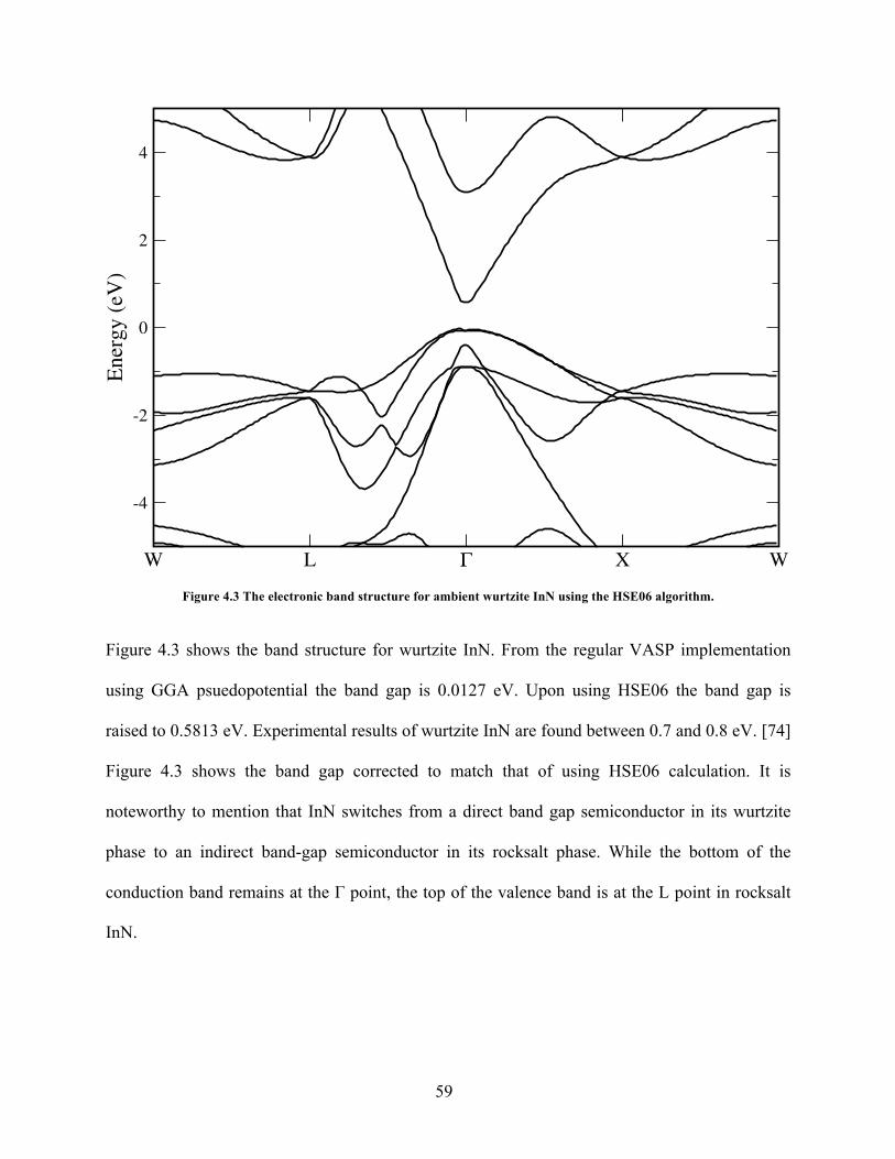
59

Figure 4.3 The electronic band structure for ambient wurtzite InN using the HSE06 algorithm.

Figure 4.3 shows the band structure for wurtzite InN. From the regular VASP implementation

using GGA psuedopotential the band gap is 0.0127 eV. Upon using HSE06 the band gap is

raised to 0.5813 eV. Experimental results of wurtzite InN are found between 0.7 and 0.8 eV. [74]

Figure 4.3 shows the band gap corrected to match that of using HSE06 calculation. It is

noteworthy to mention that InN switches from a direct band gap semiconductor in its wurtzite

phase to an indirect band-gap semiconductor in its rocksalt phase. While the bottom of the

conduction band remains at the Γ point, the top of the valence band is at the L point in rocksalt

InN.

W L Γ X W

-4

-2

0

2

4

En

erg

y (

eV)

60

Figure 4.4 Calculated phonon dispersion curves of rocksalt InN calculated at 0 (black solid line) and 13 GPa (red dashed line) and the corresponding density of states.

The phonon dispersion curves for rocksalt InN at a pressure of 0 GPa and 13 GPa are shown in

figure 4.4. These curves were achieved by calculating phonon frequencies from the force

constants as calculated by the software package Fropho. Figure 4.4 shows the dispersion for InN

with a LO-TO splitting generated using born effective charge and dielectric constant calculated

by VASP. For rocksalt InN at 0 GPa, the calculated dielectric constant is 10.632 and the Born

effective charge are 3.65600e and -3.65138e for the In and N, respectively. At 13 GPa, the

dielectric constant is 8.798 and the Born effective charge are 3.570e and -3.565e for In and N,

respectively. This phonon dispersion is similar to that of the rocksalt structure of ZnO. As shown

later in figure 4.6, many thermodynamic properties attained from the phonon frequencies show

similarities to those of ZnO discussed in chapter 3 of this thesis. Figure 4.4 also contains a

W L Γ X W0

5

10

15

20F

req

uen

cy (

TH

z)InN: 0 GPaInN: 13 GPa

0.5 1 1.5 2

PDOS

61

density of states plot. The DOS is generated with a full k-mesh as opposed to the lines of

symmetry in the phonon dispersion curve. From the DOS, we may note that a large number of

states lie in the acoustic phonon branches.

Figure 4.5 Calculated phonon dispersion curves of wurtzite InN calculated at 0 GPa.

Figure 4.5 presents a phonon dispersion curve of wurtzite InN at 0 GPa. Dielectric constant and

Born effective charge calculations were performed for wurtzite InN at 0 GPa to apply a LO-TO

splitting around Γ. As seen in experimental phonon dispersion by Davydeov et al. [79] an

appreciable LO-TO split on the Γ is observed. The dielectric constant for wurtzite InN is 9.699

for the a and b-axis and 10.496 for the c-axis. The Born effective charge along the a and b-axis

are 2.95196e for In and - 2.93900e for N. Along the c-axis the Born effective charge is 3.13048e

W L Γ X W0

5

10

15

20

Fre

quen

cy (

TH

z)

62

for In and -3.12504e for N. From this phonon dispersion curve and the phonon frequencies, we

calculate thermodynamic properties at varying temperatures.

The thermodynamic properties of rocksalt InN are calculated using the methods discussed above.

Using software package Fropho, we generate phonon frequencies that are used to calculate the

Grüneisen parameter, heat capacity, and linear thermal expansion coefficient for rocksalt InN.

The structures used for finding the phonon frequencies are from a GGA pseudopotential

containing the d-electron information.

63

Figure 4.6 Thermodynamic properties of rocksalt InN. Top: Grüneisen parameter, Middle: Heat Capacity, and Bottom: Linear thermal expansion coefficient for rocksalt InN at 0 GPa and 13 GPa and wurtzite InN at 0 GPa. The temperature

ranges from 50 K to 700 K.

100 200 300 400 500 600 700Temperature (K)

0

2

4

6

8

10

12

Hea

t Cap

acity

Cv (C

al/M

ol)

Rocksalt 0 GPaWurtzite 0 GPaRocksalt 13 GPa

100 200 300 400 500 600 700Temperature (K)

0

0.5

1

1.5

2

a

Rocksalt 0 GPaWurtzite 0 GPaRocksalt 13 GPa

100 200 300 400 500 600 700Temperature (K)

0

0.5

1

1.5

2

2.5

3

_ (1

0-5) (

Cal/G

Pa)(m

3 /K)

Rocksalt 0 GPaWurtzite 0 GPaRocksalt 13 GPa

64

Figure 4.6 shows the heat capacity, Grüneisen parameter, and linear thermal expansion

coefficient for both wurtzite and rocksalt InN at 0 GPa. Since the phonon dispersion curve for

rocksalt InN is similar to rocksalt ZnO, we have compared the two. The Grüneisen parameter

difference between InN and ZnO is about 0.8. The heat capacity difference between InN and

ZnO is 0.076 Cal/Mol at 500 K. The linear thermal expansion coefficient is about 0.9 (105)

Cal/GPa m3/K. Indeed these two materials at rocksalt phase are very similar. ZnO showed a

smaller thermal conductivity than its ambient wurtzite phase when quenched to 0 GPa. Similar to

ZnO, the results shown in figure 4.6 also suggest a small thermal conductivity, due to

anharmonic effects impeding heat transport.

We may also compare wurtzite heat capacity to measurements obtained in experiments. An

experiment by Leitner et al [80] on wurtzite InN uses Calvet calorimetry and drop calorimetry at

temperatures ranging from 300 K to 700 K. They obtained a fit of the heat capacity as a function

of temperature. From their fitting formula, at 300 K the heat capacity is 9.335 Cal per mol. This

result is similar to our calculation of 9.487 Cal per mol for wurtzite at 0 GPa at 300 K.

65

Figure 4.7 Electronic transport properties of rocksalt InN at 0 GPa. The Seebeck coefficient, electrical conductivity divided by τ , and power factor of n-type and p-type RS InN at selected temperatures from 300 K to 800 K in the carrier

concentration range of to 1× 1020 cm-3 to 1× 1022 cm-3.

1e+20 1e+21 1e+22

Hole Concentration (cm-3

)

10

100

1000

S (

µV

/K)

300 K400 K500 K600 K700 K800 K

1e+20 1e+21 1e+22

Hole Concentration (cm-3

)

1e+18

1e+19

1e+20

1e+21

σ/τ

(Ω

m s

)-1

300 K400 K 500 K600 K700 K800 K

1e+20 1e+21 1e+22

Electron Concentration (cm-3

)

1e+18

1e+19

1e+20

1e+21

σ/τ

(Ω

m s

)-1

300 K400 K 500 K600 K700 K800 K

1e+20 1e+21 1e+22

Electron Concentration (cm-3

)

10

100

1000-S

(µ

V/K

)

300 K400 K500 K600 K700 K800 K

1e+20 1e+21 1e+22

Electron Concentration (cm-3

)

0

0.01

0.02

0.03

0.04

0.05

σ S

2 (

W/m

K2)

300 K400 K500 K600 K700 K800 K

1e+20 1e+21 1e+22

Hole Concentration (cm-3

)

0

0.1

0.2

0.3

0.4

σ S

2 (

W/m

K2)

300 K400 K500 K600 K700 K800 K

66

Figure 4.8 Electronic transport properties of rocksalt InN at 13 GPa. The Seebeck coefficient, electrical conductivity

divided by τ , and power factor of n-type and p-type RS InN at selected temperatures from 300 K to 800 K in the carrier concentration range of to 1× 1020 cm-3 to 1× 1022 cm-3.

The electronic transport of InN has been investigated using software WIEN2k, BoltzTraP, and

some self-implemented codes. Figure 4.7 and 4.8 shows the Seebeck coefficient and the

electronic conductivity for rocksalt InN at 0 GPa and 13 GPa, respectively. Figure 4.7 and 4.8

1e+20 1e+21 1e+22

Electron Concentration (cm-3

)

1e+18

1e+19

1e+20

1e+21

σ/τ

(Ω

m s

)-1

300 K400 K500 K600 K700 K800 K

1e+20 1e+21 1e+22

Hole Concentration (cm-3

)

1e+18

1e+19

1e+20

1e+21

σ/τ

(Ω

m s

)-1

300 K400 K500 K600 K700 K800 K

1e+20 1e+21 1e+22

Hole Concentration (cm-3

)

0

100

200

300

400

500

S (

µV

/K)

300 K400 K 500 K600 K700 K800 K

1e+20 1e+21 1e+22

Electron Concentration (cm-3

)

0

100

200

300

400

500

S (

µV

/K)

300 K400 K 500 K600 K700 K800 K

1e+20 1e+21 1e+22

Hole Concentration (cm-3

)

0

0.05

0.1

0.15

0.2

0.25

0.3

0.35

0.4

σS

2 (

W/m

K2)

300 K, 13 GPa400 K, 13 GPa500 K, 13 GPa600 K, 13 GPa700 K, 13 GPa800 K, 13 GPa

1e+20 1e+21 1e+22

Electron Concentration (cm-3

)

0

0.01

0.02

0.03

0.04

0.05

σS

2 (

W/m

K2)

300 K, 13 GPa400 K, 13 GPa500 K, 13 GPa600 K, 13 GPa700 K, 13 GPa800 K, 13 GPa

67

are made using the energy eigenvalues generated by WIEN2k with a dense k-mesh of 48×48×48.

In addition, the WIEN2k outputs are compatible for input into BoltzTraP. Before using the

energy bands produced by WIEN2k, they are analyzed for band gap values. Using self-

implemented codes the band gap is shifted and corrected to the values found by HSE06 as

implemented by VASP. Using the shifted energy eigenvalues in the format of WIEN2k as input

for BoltzTraP various electronic transport properties may be found using the Boltzmann

transport theory.

The hole and electron concentration for both the Seebeck coefficient and electronic conductivity

divided by the relaxation time are rather similar in curvature to that from the work of Khuong P.

Ong, David J. Singh, and Ping Wu. [30] In both figure 4.7 and 4.8, which corresponds to 0 and

13 GPa rocksalt InN, respectively, the electron concentration has a lower Seebeck coefficient

than its hole concentration. This leads to the power factor, σS2, being much lower for the hole

concentration than the electron concentration.

To calculate the power factor, the relaxation time calculated with the electron conductivity must

be canceled. To do this would require an experimental data to fit the theoretical electronic

conductivity against the experimental and estimate the relaxation time from there. To our

knowledge there is yet to be experimental data on the electronic conductivity of rocksalt InN at 0

GPa. Instead an estimation of the relaxation time is made here. The relaxation time used is in the

order of 10−13 s. This value is a flat constant, however it is known that the relaxation time varies

with carrier concentration and temperature. A further investigation and improvement on these

68

electronic transport properties can made if the relaxation time and how it varies with temperature

and concentration is known.

The nudged elastic band method, NEB, is implemented in software VASP. This method is used

for finding the minimum path energy of transition states. It may also be used for diffusion of

adatom, but in this case it is used in a solid phase to solid phase transition in a material to find

the minimum energy path and the kinetic barrier associated with the path. The kinetic barrier is

determined from the saddle point. Images of the in-between stages of the transition are generated

using scripts. The atom positions of the cell are adjusted to form a linear interpolation of two

fixed end points, as for example wurtzite to rocksalt structure transition. These images are then

relaxed in all remaining degrees of freedom constrained by the interpolation. VASP calculates

the energy and the gradient of each structure with a spring between each image. A notable

difference between the nudged elastic band method and plain elastic band method is that the

force in the tangential direction of the interpolation, that is the spring force, is broken down to its

parallel and perpendicular components so that the perpendicular is projected out. This is the

“nudging” that is produced in order to achieve a correct minimum energy path.

69

Figure 4.9 Nudged elastic band calculation of WZ InN to RS InN at various pressures with 12 images, the first and last points are fixed and are the relaxed structures of wurtzite and rocksalt, respectively.

A NEB calculation was made for InN from 0 GPa up to 15 GPa for a phase transition from

wurtzite to rocksalt. This transition is hexagonal to cubic meaning the treatment of the atom

positions need to be a 1 to 1 correlation. Since the images produced are a linear interpolation,

rotations and other effects are not taken into consideration. This means for a cell of 4 atoms with

2 different atoms. There are 4 possible configurations. From the 4 configurations one must

determine which holds the lowest energy for the minimum energy path, as that path will be more

favorable in nature. Shown in figure 4.9, is the lowest energy for the minimum energy path from

those 4 configurations. Figure 4.9 gives the NEB for wurtzite to rocksalt InN at pressures up to

15 GPa. It is known that solid-to-solid phase transition nudged elastic band calculation can be

0 2 4 6 8 10 12

Images

-0.1

0

0.1

0.2

0.3E

nth

alpy (

eV/a

tom

)

0 GPa5 GPa10 GPa11 GPa12 GPa13 GPa14 GPa15 GPa

70

difficult if the end points do not have the same symmetry. [81] In this case the transition occurs

from a hexagonal to a cubic structure. The result in figure 4.9 is created from InN GGA

psuedopotential with a k-mesh of 5×5×5.

From figure 4.9, it is seen that the rocksalt phase becomes energetically more stable above a

thermal equilibrium pressure of 12 GPa, which agrees well with previous experimental results.

[77] It is also shown that the wurzite to rocksalt transition has a kinetic barrier decreasing

significantly as pressure is increased. From 0.28/atom eV at 0 GPa reduced to 0.15 eV/atom at

12 GPa. This allows for kinetic phase fluctuations and for the atoms in a wurtzite structure to

move about and find a more energetically favorable rocksalt structure at higher pressures.

IV. CONCLUSIONS

We are still unaware if these materials can be quenched and remain stable under ambient

conditions. There are some experimental studied that have found rocksalt InN to be quenchable

to around 3 GPa [18]. With improving techniques in epitaxial growth, this material’s high-

pressure phase may very well be produced at ambient conditions. However, here we show good

results from this research and possible applications as a semiconducting material. We can

satisfactorily conclude that the results are within range of experimental and other theoretical

results. Our transition pressure, figure 4.1 and 4.9, and band gap, figure 4.2, are near to

experimental results. We show transport properties, Seebeck coefficient and conductivity, of the

high-pressure phase at 0 and 13 GPa. The thermodynamic properties of InN are also shown and

calculated from the phonon frequencies. The results of which suggest a low thermal conductivity

and a promising thermoelectric material. Continuing work is being made to gather a satisfactory

71

thermal conductivity and more accurate relaxation time for applications as a thermoelectric

material and develop a figure of merit ZT.

72

Chapter 5

PHASE-TRANSITION INDUCED GAP TRANSITION

IN PbS

I. INTRODUCTION

Lead chalcogenides (PbX, X= S, Se, Te) are a class of narrow band gap semiconductors that are

widely used for infrared detectors, diodes, thermoelectric devices and thermophotovoltaic

converters. [82-84] Anomalous ferroelectric fluctuations [85, 86] and large anharmonic phonon

scattering [87,88] in PbX have recently been discovered and are theoretically attributed to

competitive bonding between ionicity and covalency. [89] In ambient conditions, these materials

crystallize in the rocksalt (RS) structure. They transition to an orthorhombic structure at around

2-6 GPa and further transition into a Caesium Chloride (CsCl) structure from 13-20 GPa [90-97].

The transition from RS to orthorhombic to CsCl structures is attributed to an electronic

transformation from semiconductor to semiconductor to metal. [84,98] However, it is

experimentally challenging to accurately determine electronic properties of the orthorhombic and

CsCl phases at high pressures; as a result, they have been the subject of debate and controversy.

[84, 95, 97−99] In fact, pressure-induced phase transition between RS and CsCl structures has

also been observed in binary pnictides (e.g., CeP and CeAs), [100, 101] halides (e.g., NaCl and

KCl), [102] and hydrides (e.g., NaH and KH). [103,104] A thorough overview of the RS to CsCl

transition can be found in [105]. Thus, the study of the structural transition between RS and CsCl

is of a fundamental and technological importance.

73

The structure of intermediate phase is a key to understanding the pressure-induced RS to CsCl

transitions. In most material systems the RS-CsCl transition proceeds without involvement of

any intermediate phase. [105] As exceptions, only a few materials have an intermediate phase.

For the case of AgF and NpAs, hexagonal structures are the intermediate phase between the RS

to CsCl transitions in. [106, 107] An isostructural transition is observed for SmTe and EuO

before transforming to a CsCl type structure at higher pressures. [108] For the cases of lead

chalcogenides, the GeS-type Pnma [84, 92] and InI-type Cmcm [89, 93] structures have both

been reported as intermediate phases on the basis of high-pressure synchrotron X-ray diffraction.

To complicate the matter further, a new orthorhombic phase, neither of GeS- and InI-type

structures, has been reported as an intermediate phase in PbTe at 6 GPa. [90] However many

reports have been made to suggest two possible orthorhombic phases are of GeS-type and InI-

type. [109-111] Previous first-principles calculations on the structures of the orthorhombic phase

have also been performed, but the results are as conflicting as the experimental reports. [98, 99,

112, 113] In addition, there are significant discrepancies in the elastic bulk modulus (B0)

determined for orthorhombic PbS. The B0 value measured by Grzechnik et al., for example, is

134(2) GPa, [94] which is more than 300% larger than that reported by Knorr et al., which is

30.9(4) GPa. [93] A similar discrepancy can also be found in ab-initio simulations. [93, 112]

In this chapter, first-principles calculations are made to study crystal structures, phase stability,

elastic and electronic properties of PbS. This study is also in corroboration with an experimental

study and is used for theoretical support in the form of ab-intio simulations [5]. Shown below are

only those first-principles calculations made by the author of this thesis.

74

II. METHOD OF CALCULATIONS

First-principles calculations were performed for PbS using the generalized gradient

approximation (GGA-PBE) [15] implemented in the VASP package. [20] The projector

augmented-wave (PAW) [21] and pseudopotential methods were employed with a plane-wave

basis set, which was truncated at the cutoff energy of 400 eV to obtain a 0.2 meV convergence in

the total energy per atom. The Brillouin zone integration was carried out with a 16 × 16 × 16 k-

point grid generated by the Monkhorst−Pack algorithm. [24] The final energy convergence for

electronic steps is in the magnitude of 1 µeV. The force convergence of ionic steps was set to be

10 µeV/Å. The spin-orbital interaction was involved for band structure calculations.

III. RESULTS AND DISCUSSION

Using the inputs discussed above, a relaxed structure is generated for three structures, the cubic

RS structure and the two possible orthorhombic phases Pmna (B16) and Cmcm (B33). Their

transition pressures are found and shown by the enthalpy versus pressure plot in figure 5.1. The

transition pressures for cubic to the orthorhombic structures are 8.5 GPa for Cmcm and 9.8 GPa

for Pmna. These results are higher than the experimental measurements, which find a transition

at about 2.1 GPa [5]. As seen in figure 5.1, Cmcm is energetically more favorable than Pmna,

and it can be said that PbS is isotypic with indium iodide InI and adopts its structure Cmcm.

75

Figure 5.1 Calculated pressure dependence of the enthalpy difference between both orthorhombic phases and the cubic phase.

A pressure versus volume plot is also generated and shown in figure 5.2. The third-order

Birch−Murnaghan equation of state [113] was fitted to derive the bulk modulus B0. The bulk

modulus from the calculation is 55 GPa and 24 GPa for cubic and orthorhombic Cmcm phase,

respectively, which agrees well with previously reported values. [5, 93, 98] This result finds that

the orthorhombic phase is about 50% more compressible than the low-pressure cubic phase. This

goes against common intuition that a material under pressure will become less and less

compressible. It is shown that after the phase transition, this is not true for PbS. The result is

76

quite anomalous, yet consistent with the experimental data provided for PbS that there is a phase

transition induced elastic softening.

Figure 5.2 Pressure versus volume curve with calculated bulk modulus of cubic and two orthorhombic phases of PbS.

Lastly, the electronic structure of the cubic and the InI-type Cmcm orthorhombic phases were

calculated. Figure 5.3 shows the electronic band structure along with the DOS for both

structures. As shown in Figure 5.3, the two phases show remarkable differences in their band

structures and total density of states (DOS) at the Fermi energy level. It can be seen that he cubic

phase is a direct band gap semiconductor. That is that the top of the valence band and bottom of

the conduction band occur at the same L symmetry point (see Figure 5.3 a). The obtained band

gap, Eg, is 0.47 eV, which is close to the experimental value of 0.42 eV at 300 K [114, 57] and a

reported theoretical result [98]. The orthorhombic phase has an indirect band gap of Eg = 1.04 eV

0 5 10 15 20 25 30Pressure (GPa)

0.7

0.75

0.8

0.85

0.9

0.95

1

V/V

0

PbS-CubicPbS-PnmaPbS-Cmcm

B0 = 55.20

B0 = 30.66

B0 = 24.21

77

(see figure 5.3 b) and is similar to that of the silicon semiconductor with a band gap of Eg = 1.11

eV at 300 K. [115] The simulations show there is a direct-to-indirect band gap transition induced

by a phase transition in semiconducting PbS. An observation made by [5] also sees an abrupt

increase in electrical resistivity measurements during transition, which supports band gap

transition.

Figure 5.3 Electronic band structure of cubic (a) and orthorhombic Cmcm (b) PbS (upper panel) and the total density of

state DOS (lower panel). The cyan dashed line represents the Fermi energy E = 0 eV.

IV. CONCLUSION

In summary, the pressure-induced phase transition in PbS was studied by first-principles

calculations. Two possible orthorhombic configurations are considered. Of the two, Cmcm is

78

energetically more favorable. Both cubic and orthorhombic phases are semiconductors, but they

exhibit features of direct and indirect band gaps, respectively, with Eg = 0.47 and 1.04 eV. Phase

transition induced elastic softening is shown using calculated Birch−Murnaghan equation of state

that the orthorhombic phase is more compressible than the cubic phase. Phase transition also

leads to an anomalous drop in electrical conductivity in orthorhombic PbS, which is mainly

attributed to the enlarged and indirect band gap in the Cmcm phase as well as the lower crystal

symmetry when compared to cubic.

79

REFERENCES

1. C. H. Bates, W. B. White, and R. Roy, Science 137, 993 (1962).

2. I.G. Pichugin, M. Tiachala, Izv. Akad. Nauk SSSR, Neorg. Mater. 14, 175 (1978).

3. P. S. Sokolov, A. N. Baranov, Zh. V. Dovrokgotov, and V. L. Solozhenko, Russ. Chem.

Bull. 59, 325 (2010).

4. J. Ibaez, A. Segura, F. j. Manjon, L. Artus, T. Yamaguchi, and Y. Nanishi, Appl. Phys.

Lett. 96, 201903 (2010).

5. S. Wang, J. Zhang, Y. Zhang, A. Alvarado, J. Attapattu, H. Duanwei, L. Wang, C. Chen,

and Y. Zhao, Inorg. Chem. 52, 8638-8643 (2013).

6. N. W. Ashcroft and N. D. Mermin, Solid State Physics (1976).

7. C. Kittel, Introduction to Solid State Physics (1991).

8. Max Born and Robert Oppenheimer, Zur quantentheorie der molekeln. In: Annalen der

Physik 389, 457–484 (1927).

9. P. Hohenberg and W. Kohn, Phys. Rev. 136, B864 (1964).

10. W. Kohn and L. J. Sham Phys. Rev. 140, A1133–A1138 (1965).

11. J. P. Perdew and A. Zunger, Phys. Rev. B 23, 5048–5079 (1981).

12. J. P. Perdew and Y Wang, Phys. Rev. B 45, 13244–13249 (1992).

13. NM Harrison, An introduction to density functional theory. NATO SCIENCE SERIES

SUB SERIES III COMPUTER AND SYSTEMS SCIENCES 187, 45–70 (2003).

14. J. P. Perdew, J. A. Chevary, S. H. Vosko, Koblar A. Jackson, Mark R. Pederson, D. J.

Singh, and C. Fiolhais Phys. Rev. B 46, 6671 (1992).

15. J. P. Perdew, K. Burke, and M. Ernzerhof Phys. Rev. Lett. 77, 3865 (1996).

80

16. J. Tao, J. P. Perdew, V. N. Staroverov, and G. E. Scuseria Phys. Rev. Lett. 91 146401

(2003).

17. P. J. Stephens, F. J. Devlin, C. F. Chabalowski, and M. J. Frisch J. Phys. Chem. 98,

11623 (1994).

18. H. Hellmann, Einführung in die Quantenchemie. Leipzig: Franz Deuticke 285, (1937).

19. R. P. Feynman Phys. Rev. 56, 340 (1939).

20. G. Kresse and J. Furthmller, Phys. Rev. B 54, 11169 (1996).

21. G. Kresse and D. Joubert, Phys. Rev. B 59, 1758 (1999).

22. P. Pulay, Chem. Phys. Lett. 73, 393 (1980).

23. W.H. Press, B.P. Flannery, S.A. Teukolsky and W.T. Vetterling, em Numerical Recipes

(Cambridge University Press, New York, 1986).

24. H.J. Monkhorst und J.D. Pack, Phys. Rev. B 13, 5188 (1976).

25. P. Blaha, K. Schwarz, G. Madsen, D. Kvasnicka, and J. Luitz, WIEN2k, An Augmented

Plane Wave + Local Orbitals Program for Calculating Crystal Properties (Technische

Universit€at Wien, Austria, 2001).

26. David Singh Phys. Rev. B 43, 6388 (1991).

27. D. Singh and L. Nordstrom, Plane waves, pseudopotentials and the LAPW method, (2nd

edition, Springer, New York, 2006).

28. Kaye, G W. C, and T H. Laby. Tables of Physical and Chemical Constants: And Some

Mathematical Functions, (Wiley, New York, 1966).

29. G. K. H. Madsen, D. J. Singh, Comput. Phys. Commun. 175, 67 (2006).

30. K. P. Ong, D. J. Singh, and P. Wu, Phys. Rev. B 83, 115110 (2011).

31. A. Togo, F. Oba, and I. Tanaka, Phys. Rev. B 78, 134106 (2008).

81

32. K. Parlinski, Z. Q. Li, and Y. Kawazoe Phys. Rev. Lett. 78, 4063 (2007).

33. Ü Özgür, Ya. I. Alivov, C. Liu, A. Teke, M. A. Reshchikov, S. Dogan, V. Avrutin, S. J.

Cho, and H. Morkoc, J. Appl. Phys. 98, 041301 (2005).

34. W. Class, A. Ianucci, and H. Nesor, Norelco Rep. 13, 87 (1966).

35. M. Ohtaki, T. Tsubota, K. Eguchi, and H. Arai, J. Appl. Phys. 79, 1816 (1996).

36. J. P. Wiff, Y. Kinemuchi, H. Kaga, C. Ito, and K. Watari, J. Eur. Ceram. Soc. 29, 1413

(2009).

37. J. P. Wiff, Y. Kinemuchi, and K. Watari, Mater. Lett. 63, 2470 (2009).

38. M. Ohtaki, K. Araki, and K. Yamamoto, J. Electron. Mater. 38, 1234 (2009).

39. B. A. Cook, J. L. Harringa, and C. B. Vining, J. Appl. Phys. 83, 5858 (1998).

40. Y. Kinemuchi, C. Ito, H. Kaga, T. Aoki, and K. Watari, J. Mater. Res. 22, 1942 (2007).

41. M. Ueno, Y. Yoshida, Y. Takai, and M. Yamaguchi, J. Ceram. Soc. Jpn. 112, 327 (2004).

42. T. Tsubota, M. Ohtaki, K. Eguchi, and H. Arai, J. Mater. Chem. 8, 409 (1998).

43. T. Tsubota, M. Ohtaki, K. Eguchi, and H. Arai, J. Mater. Chem. 7, 85 (1997).

44. S. Katsuyama, Y. Takagi, M. Ito, K. Majima, H. Nagai, H. Sakai, K. Yoshimura, and K.

Kosuge, J. Appl. Phys. 92, 1391 (2002).

45. Y. Fujishiro, M. Miyata, M. Awano, and K. Maeda, J. Am. Ceram. Soc. 87, 1890 (2004).

46. K. H. Kim, S. H. Shim, K. B. Shim, K. Nihara, and J. Hojo, J. Am. Ceram. Soc. 88, 628

(2005).

47. H. Kaga, Y. Kinemuchi, S. Tanaka, A. Makiya, Z. Kato, K. Uematsu, and K. Watariet,

Jpn. J. Appl. Phys., Part 2 45, L1212 (2006).

48. S. Isobe, T. Tani, Y. Masuda, W. S. Seo, and K. Kuomoto, Jpn. J. Appl. Phys., Part 1 41,

731 (2002).

82

49. S. J. Pearton, D. P. Norton, K. Ip, Y. W. Heo, and T. Steiner, Prog. Mater. Sci. 50, 293

(2005).

50. D. C. Look, Mater. Sci. Eng., B 80, 383 (2001).

51. P. Zu, Z. K. Tang, G. K. L. Wong, M. Kawasaki, A. Ohtomo, K. Koinuma, and Y.

Sagawa, Solid State Commun. 103, 459 (1997).

52. D. M. Bagnall, Y. R. Chen, Z. Zhu, T. Yao, S. Koyama, M. Y. Shen, and T. Goto, Appl.

Phys. Lett. 70, 2230 (1997).

53. M. Wraback, H. Shen, S. Liang, C. R. Gorla, and Y. Lu, Appl. Phys. Lett. 74, 507 (1999).

54. J. M. Lee, K.-K. Kim, S. J. Park, and W.-K. Choi, Appl. Phys. Lett. 78, 2842 (2001).

55. J. E. Nause, III-V’s Rev. 12, 28 (1999).

56. Y. Chen, D. Bagnall, and T. Yao, Mater. Sci. Eng., B 75, 190 (2000).

57. Y. Zhang, X. Ke, C. F. Chen, J. Yang, and P. R. C. Kent, Phys. Rev. B 80, 024304

(2009).

58. J. M. Ziman, Electrons and Phonons (Oxford University Press, New York, 2001).

59. Y. Zhang, J. Dong, P. R. C. Kent, J. Yang, and C. F. Chen, Phys. Rev. B 92, 020301(R)

(2015).

60. X. Tang and J. Dong, Proc. Natl. Acad. Sci. U.S.A. 107, 4539 (2009).

61. K. Esfarjani, G. Chen, and H. T. Stokes, Phys. Rev. B 84, 085204 (2011).

62. H. Karzel, W. Potzel, M. Kfferlein, W. Schiessl, M. Steiner, U. Hiller, G. M. Kalvius, D.

W. Mitchell, T. P. Das, P. Blaha, K. Schwarz, and M. P. Pasternak, Phys. Rev. B 53,

11425 (1996).

63. L. Gerward and J. S. Olsen, J. Synchrotron Radiat. 2, 233 (1995).

64. J. E. Jaffe and A. C. Hess, Phys. Rev. B 48, 7903 (1993).

83

65. A. Segura, J. A. Sans, F. J. Manjón, A. Muñoz, and M. J. Herrera-Cabrera, Appl. Phys.

Lett. 83, 278 (2003).

66. T. Olorunyolemi, A. Birnboim, Y. Carmel, O. C. Wilson, Jr., and I. K. Lloyd, J. Am.

Ceram. Soc. 85, 1249 (2002).

67. S. Katayama, H. Hayashi, F. Oba, and I. Tanaka, Jpn. J. Appl. Phys., Part 1 50, 075503

(2011).

68. R. S. Koster, C. M. Fang, M. Dijkstra, A. van Blaaderen, and M. A. van Huis, J. Phys.

Chem. C 119, 5648 (2015).

69. S. W. H. Eijt, J. de Roode, H. Schut, B. J. Kooi, J. Th., and M. De Hosson, Appl. Phys.

Lett. 91, 201906 (2007).

70. H. Morko, Nitride Semiconductors and Devices (Springer, New York, 1999).

71. T. Inushima, V. V. Mamutin, V. A. Vekshin, S. V. Ivanov, T. Sakon, M. Motokawa, and

S. Ohoya, J. Cryst. Growth 227/228, 481 (2001).

72. V. Yu. Davydov et al., Phys. Status Solidi B 230, R4 (2002); 229, R1 (2002); 234, 787

(2002).

73. J. Wu et al., Appl. Phys. Lett. 80, 3967 (2002).

74. J. Wu, W. Walukiewicz, K. M. Yu, J. W. Ager III, E. E. Haller, H. Lu, and W. J. Schaff,

Appl. Phys. Lett. 80, 4741 (2002).

75. A. Yamamoto, K. Sugita, H. Takatsuka, A. Hashimoto, and V. Yu. Davydov, J. Cryst.

Growth 261, 275 (2004).

76. T. L. Tansley and C. P. Foley, J. Appl. Phys. 59, 3241 (1986).

77. C. Pinquier et al., Phys. Rev. B 73, 115211 (2006).

78. I. Vurgaftman, J. R. Meyer, and L. R. Ram-Mohan, J. Appl. Phys. 89, 5815 (2001).

84

79. V. Yu. Davydov, et al., Appl. Phys. Lett 75, 3297 (1999).

80. J. Leitnera, P. Marka, et al., Journal of Physics and Chemistry of Solids, 65, 1127 (2004).

81. D. Sheppard, P. Xiao, W. Chemelewski, D. D. Johnson, and G. Henkelman, J. Chem.

Phys. 136, 074103 (2012).

82. D. Khokhlov, Lead Chalcogenides: Physics and Applications; (Taylor & Francis, New

York, 2002).

83. Y. Z. Pei, A. LaLonde, S. Iwanaga, and G. J. Snyder, Energy Environ. Sci. 4, 2085−2089,

(2011).

84. S. V. Ovsyannikov, V. V. Shchennikov, S. V. Popova, and A. Y. Derevskov, Phys. Status

Solidi B 235, 521−525, (2003).

85. E. S. Bozin, C. D. Malliakas, P. Souvatzis, T. Proffen, N. A. Spaldin, M. G. Kanatzidis,

and S. J. L. Billinge, Science 330, 1660− 1663, (2010).

86. K. M. Ø. Jensen, E. S. Bozin, C. D. Malliakas, M. B. Stone, M. D. Lumsden, M. G.

Kanatzidis, S. M. Shapiro, and S. J. L. Billinge, Phys. Rev. B 86, 085313 (2012).

87. O. Delaire, J. Ma, K. Marty, A. F. May, M. A. McGuire, M. H. Du, D. J. Singh, A.

Podlesnyak, G. Ehlers, M. D. Lumsden, and B. C. Sales, Nat. Mater. 10, 614−619 (2011).

88. Y. Zhang, X. Ke, P. R. C. Kent, J. Yang, and C. Chen, Phys. Rev. Lett. 107, 175503

(2011).

89. T. Chattopadhyay, H. G. Vonschnering, W. A. Grosshans, and W. B. Holzapfel, Phys. B

& C 139, 356−360 (1986).

90. G. Rousse, S. Klotz, A. M. Saitta, J. Rodriguez-Carvajal, M. I. McMahon, B. Couzinet,

and M. Mezouar, Phys. Rev. B 71, 224116 (2005).

85

91. Y. Fujii, K. Kitamura, A. Onodera, and Y. Yamada, Solid State Commun. 49, 135−139

(1984).

92. I. Wakabaya, H. Kobayash, H. Nagasaki, and S. J. Minomura, Phys. Soc. Jpn. 25,

227−233 (1968).

93. K. Knorr, L. Ehm, M. Hytha, B. Winkler, and W. Depmeier, Eur. Phys. J. B 31, 297−303

(2003).

94. A. Grzechnik, and K. J. Friese, Phys. Condens. Matter 22, 095402 (2010).

95. J. Z. Jiang, L. Gerward, R. Secco, D. Frost, J. S. Olsen, and J. J. Truckenbrodt, Appl.

Phys. 87, 2658−2660 (2000).

96. D. W. Fan, W. G. Zhou, S. Y. Wei, J. Liu, Y. C. Li, S. Jiang, and H. S. Xie, Chin. Phys.

Lett. 27, 086401 (2010).

97. K. T. Wheeler, D. Walker, and M. C. Johnson, Am. J. Sci. 307, 590−611 (2007).

98. R. Ahuja, Phys. Status Solidi B 235, 341−347 (2003).

99. D. Zagorac, K.; Doll, J. C. Schön, and M. Jansen, Phys. Rev. B 84, 045206 (2011).

100. I. Vedel, A. M. Redon, J.; Rossatmignod, O. Vogt, and J. M. J. Leger, Phys. C Solid State

Phys. 20, 3439−3444 (1987).

101. A. Werner, H. D. Hochheimer, and R. L. Meng,E.Bucher, Phys. Lett. A 97, 207−209

(1983).

102. L. J. Merrill, Phys. Chem. Ref. Data 6, 1205−1252 (1977).

103. S. J. Duclos, Y. K. Vohra, A. L. Ruoff, S. Filipek, and B. Baranowski, Phys. Rev. B 36,

7664−7667 (1987).

104. H. D. Hochheimer, K. Strossner, W. Honle, B. Baranowski, and F. J. Filipek, Less-

Common Met. 107, L13−L14 (1985).

86

105. P. Toledano, K. Knorr, L. Ehm, and W. Depmeier, Phys. Rev. B 67, 144106 (2003).

106. J. C. Jamieson, P. M. Halleck, R. B. Roof, and C. J. Pistorius, Phys. Chem. Solids 36,

939−944 (1975).

107. U. Benedict, S. Dabosseignon, C. Dufour, H. Luo, and S. J. Heathman, Nucl. Mater. 166,

48−55 (1989).

108. A. Jayaraman, A. K. Singh, A. Chatterjee, and S. U. Devi, Phys. Rev. B 9, 2513−2520

(1974).

109. T. Yagi, T. Suzuki, and S. J. Akimoto, Phys. Chem. Solids 44, 135−140 (1983).

110. G. A. Samara, L. C. Walters, and D. A. J. Northrop, Phys. Chem. Solids 28, 1875−1883

(1967).

111. K. Kusaba, Y. Syono, T. Kikegawa, and O. J. Shimomura, Phys. Chem. Solids 56,

751−757 (1995).

112. Y. Bencherif, A. Boukra, A. Zaoui, and M. Ferhat, Mater. Chem. Phys. 126, 707−710

(2011).

113. F. Birch, Phys. Rev. 71, 809−824 (1947).

114. I. Madelung, O. Rössler, U. Schulz, M. Eds. In Non-Tetrahedrally Bonded Elements and

Binary Compounds, 41C, 1−4 (Springer: Berlin, Germany, 1998).

115. V. Alex, S. Finkbeiner, and J. J. Weber, Appl. Phys. 79, 6943− 6946 (1996).

87

CURRICULUM VITAE

THE GRADUATE COLLEGE

UNIVERSITY OF NEVADA, LAS VEGAS

ANDREW ALVARADO

EMAIL: ALVAR170@UNLV.NEVADA.EDU

Education

M.S. in Physics (2014 – May 14, 2016) University of Nevada, Las Vegas B.S. in Physics (2010-2014) University of Nevada, Las Vegas

Awards and Activities

Millennium Scholarship 2010 - 2014

Rebel Achievement Scholarship 2010 – 2014

Nevada Space Grant Scholarship 2012 – 2013

Nevada Space Grant Scholarship 2013 – 2014

Graduate Assistantship Fellowship 2014 - 2016

UNLV Dean’s Honor List 2012, Fall 2013, Spring 2014

88

Professional Experience

Graduate Research 2014 - 2016 I work in a highly distributed Linux based environment and develop programs using C++, Fortran, and shell script. I created several C++ programs that do data analysis using parallel computations, and have developed programs for visualization of the data. One of my finished projects involves high-pressure thermoelectric properties of ZnO. The project involved planning the research, effective use of computation expenses, writing several C++ programs for data analysis, using several software packages, and reading scientific literature.

As a graduate researcher, I teach introductory physics labs and teach new members of the research group fundamentals of computational analysis.

Undergraduate Research 2011 - 2014 Co-authored in a paper that studies high-pressure properties of PbS [S. Wang et al., Inorganic Chemistry 52, 8638 (2013)]. This project involved using VASP and self-developed codes to calculate structural properties of PbS. I calculated phase transitions, band-gaps, bulk modulus, and visualized the band structure and phonon dispersion curve for PbS.

Lab Instructor 2014 – 2016 I have taught several introductory lab courses. I am responsible for teaching the students how to safely use lab equipment and how to conduct a scientific experiment.

Other Experiences

Volunteer Safety Nights 2006 – 2010 I volunteered for safety nights where young children can socially interact in a safe environment. I monitored the room and cleaned up.

Volunteer Middle School Science Bowl 2015 I volunteered for a middle school science bowl, young and brilliant students compete with each other for a chance to move on to the national science bowl. I monitored the room and made sure important packages were received to a head administrator.

Volunteer Skybot Challenge 2015 I volunteered for the first ever Skybot challenge where young aspiring scientists can compete with their own drones in rigorous obstacle courses. I was a referee and scorekeeper for the competitions.

89

Professional Associations

Member of HiPSEC.

Member of UNLV’s Society of Physics Students.

Student member of the American Physics Society (APS).

Advanced Photon Source user at Argonne National Lab.

Publications

Shanmin Wang, Jianzhong Zhang, Yi Zhang, Andrew Alvarado, Jeevake Attapattu, Duanwei He, Liping Wang, Changfeng Chen, and Yusheng Zhao, Inorg. Chem. 52, 8638 (2013). Andrew Alvarado, Jeevake Attapattu, Yi Zhang, and Changfeng Chen, J. Appl. Phys. 118, 165101 (2015).

Presentations

NNSA SSAP Symposium Bethesda, Maryland 2016 High-pressure properties of rocksalt InN from first-principles calculation Graduate Poster presentation for those affiliated with NNSA.

HiPSEC annual review Las Vegas, Nevada 2015 Thermoelectric properties of rocksalt ZnO from first-principles calculation Graduate poster presentation for those involved in HiPSEC for annual review.

NNSA SSAP Symposium Santa Fe, New Mexico 2015 Thermoelectric properties of rocksalt ZnO from first-principles calculation Graduate poster presentation for those affiliated with NNSA.

NSTec/UNLV Symposium Las Vegas, Nevada 2014 Thermoelectric properties of rocksalt ZnO from first-principles calculation Undergraduate poster presentation for those affiliated with NSTec and UNLV.

APS March Meeting Denver, Colorado 2014 Thermoelectric properties of rocksalt ZnO from first-principles calculation Undergraduate poster presentation for the American Physical Society on my work on ZnO

Recent/Current Research

Electronic Structure calculations of PbS from first-principles 2013 Using VASP I conducted calculations and simulations on the lattice structure and the electronic structure of PbS to find parameters such as lattice parameter, Band-gap, Density of States, and the transition pressure.

90

Thermoelectric properties of rocksalt ZnO from first-principles 2014-2015 I used first-principles methods to calculate phonon transport, from which I obtained heat capacity, Grüneisen parameter, group, velocity and phonon relaxation time. These results allowed determination of thermal conductivity at varying temperatures. I also calculated the electronic band structure of RS-ZnO and determined Seebeck coefficient and electric conductivity as a function of temperature and carrier concentration. From the transportation properties I calculated the figure of merit ZT.

High Pressure properties of novel materials from first-principles 2014-2016 Using software package VASP, WIEN2k, BoltzTraP, Fropho, and self implemented codes I study the electronic and heat transport properties of compounds: InN, InAs, and InP. Thermodynamic properties are calculated through phonon frequencies from Boltzmann transport theory as implemented by Fropho and self developed codes. Electronic transport properties, band-gaps, Seebeck coefficient, and electronic conductivity, are calculated through electronic energy eigenvalues as implemented by VASP, WIEN2k, BoltzTraP, and self developed codes. Phase transitions and minimization of energy paths are analyzed through the use of nudged elastic band method.

Skills

• Thorough understanding in use of scientific software VASP (structure relaxation, elastic properties, electronic band structure, phase transitions), BoltzTrap (Electronic transport: Seebeck coefficient, electrical conductivity), Fropho (phonon transport, dispersions and density of states), and WIEN2K (electronic transport, energy bands, and structure relaxation).

• Savvy in computer languages C++, Fortran, Java, HTML. Created several programs to calculate physical properties including a calculation of thermodynamic lattice properties from phonons.

• Skilled in Microsoft Word, Excel, PowerPoint, Latex, Xmgrace, and other similar software. • Fluent in Spanish.