high pressure viscosity measurement with falling body … pressure viscosity measurement... · the...

International Review of Chemical Engineering (I.RE.CH.E.), Vol. 2, N. 5

September 2010

Manuscript received and revised August 2010, accepted September 2010 Copyright © 2010 Praise Worthy Prize S.r.l. - All rights reserved

564

High Pressure Viscosity Measurement with Falling Body Type Viscometers

Carl J. Schaschke

Abstract – With the increasing number of applications of high pressure chemical and process technologies across a range of engineering fields, there is a corresponding growing interest in the need to measure accurately and reliably important rheological parameters. Of these, the measurement of good and reliable viscosity data is critical in engineering design. The ability to measure viscosity at high pressure, however, presents a number of engineering challenges and a number of innovative viscometers have consequently been devised and operated. This review considers those devices which are based on the falling body principle and considers falling ball, cylinder and needle in open and closed systems. Viscosity is determined from the rate of fall and the usual challenge is to detect its position during descent. While reliable data can be obtained from these viscometers, there is a discrepancy between theoretical values and actual values. This is the result of end effects in the form of vortices, wake oscillations and shedding. Calibration is therefore necessary in all cases. Improvements to analytical models have been attempted and computation fluid dynamics is also used to examine in more detail the flow fields around bodies to understand and appreciate better the performance of these viscometers. Copyright © 2010 Praise Worthy Prize S.r.l. - All rights reserved. Keywords: Falling Body Viscometer, High Pressure, Viscosity, Density, CFD

Nomenclature A Flow area (mm2) A Calibration constant (mPa s-1) Ao Constant at infinite viscosity (mPa s-1) B Coefficient C Sinker coefficient CD Drag coefficient (-) de Equivalent hydraulic diameter (mm) dp Diameter of a particle (mm) ds Sinker diameter (mm) d Inner diameter viscometer tube (mm) e Eccentric displacement from centreline (mm) g Gravitational acceleration (m s-2) G Eccentricity factor (-) Ge Geometric index (-) Ls Length of sinker (mm) Lt Distance of tube between coils (mm) k Sinker dimensionless radius (r1/ r2) m Mass of sinker (g) n Calibration exponent (-) p Pressure (N m-2) pref Reference pressure (N m-2) P Wetted perimeter (mm) Q Rate of flow (m3 s-1) r General radius (mm) r1 Radius of sinker (mm) r2 Inner radius of viscometer tube (mm) rmax Radius corresponding to du/du=0 (mm)

Rep Reynolds number for a particle (-) Rem Modified Reynolds number (-) t Sinker fall time (s) T Temperature (K) Tref Reference temperature (K) us Terminal velocity of sinker (m s-1) u Liquid velocity, m s-1 vt Terminal velocity of sinker, m s-1

z Vertical coordinate ∆V Change in voltage (V)

Greek

α Thermal expansion (coef. thermal expansion K-1) α Constant in equation 26 (MPa-1) β Bulk compressibility (MPa-1) µ Viscosity (mPa s) µo Viscosity at ambient conditions (mPa s) ρl Liquid density (kg m-3) ρs Sinker density (kg m-3) τ Shear stress (N m-2)

I. Introduction Understanding the flow behaviour of fluids is

fundamental to virtually every aspect of chemical and process engineering. The study of fluid flow, sometimes known as transport phenomena or fluid mechanics deals with the behaviour of fluids when subjected to changes

Carl J. Schaschke

Copyright © 2010 Praise Worthy Prize S.r.l. - All rights reserved International Review of Chemical Engineering, Vol. 2, N. 5

565

of pressure, frictional resistance, flow through various types of duct, orifice and nozzle, impact of jets and production of power. It also includes the development and testing of theories devised to explain the various phenomena that occur.

The study of fluids is of great importance in the chemical and process industries. Process materials, whether they be solids, liquids, gases, or some mixture of these phases, are transported from one place to another via pipes, ducts or channels. Process plants may feature many hundreds of kilometres of pipework. To transport the fluids along the pipework requires energy, which, in turn, translates to a financial cost. A full appreciation, knowledge and understanding of the nature of fluids therefore allows cost-effective design and operation of pipework and operations such as packed towers, fluidised beds, safety relief systems, fluid flow metering and control etc. These flows may be either laminar or turbulent, compressible or incompressible, single or multi-phase, or multi-component, Newtonian or non-Newtonian in nature.

While fluids may be described as substances which offer no resistance to shear and include both gases and liquids, gases differ from liquids in that they are compressible and may be described by simple gas laws. Liquids, on the other hand, are effectively classified as being incompressible, and for most practical purposes their density remains constant. This, however, is not strictly true. Water, for example, has a 3.3% compressibility at pressures of 69 MNm-2.

The measurement of fluid of process fluids is an essential aspect of any process operation, not only for plant control and safety but also for fiscal purposes. Both viscosity and density are essential parameters which define the nature of fluid flow behaviour. Viscosity is the phenomenon in which a liquid will withstand a slight amount of tension due to molecular tension between the particles, which will cause an apparent shear resistance between two adjacent layers. Density is the mass per unit volume. Fluids may be classified as incompressible or compressible, depending upon whether the density is constant or a function of pressure.

Over the past decade or so, there has been an increasing commercial and industrial interest in the application of high pressure technology in the processing of fluids. A wide range of foods, for example, are now being processed world-wide using high pressure technology principally as a non-thermal alternative to extending shelf life. The technology also provides the food industry with a plethora of new product development opportunities that is able to exploit the functional properties of ingredients such as hydrocolloids and proteins. High pressure technology is proving increasingly attractive and beneficial in the destruction of micro-organisms, activation and deactivation of enzymes, inactivation kinetics of both vegetative and pathogenic microorganisms, change of functional properties of biopolymers such as proteins and

polysaccharides used in foams, gels and emulsions, and the control of phase change such as fat solidification and ice melting point [1] [2].

The application of high pressure is not new and has long been used in a number of industrialised areas including the production of plastics, ceramics, metal-forming and pharmaceutical tablet manufacture. Many diesel-powered vehicles these days operate with high pressure common rail diesel engine systems. Unlike their petrochemical counterpart, diesel and biodiesel blends are expected to function through compressive combustion in which high pressure injection enables rapid atomisation and combustion to provide higher efficiencies and reduction in emissions [3]. Understanding the transport behaviour of these fuels is critical in the safe and efficient design, and performance of these engines. Under the extreme high pressure conditions used both density and viscosity vary significantly, and at a certain point hydrocarbon fuels will pressure-freeze. At low ambient temperature diesel and biodiesel are also known to wax and solidify, which is a major issue particularly in the colder climes [4].

II. Viscosity Measurement The measurement of viscosity can be determined by

applying a known shear force and measuring the resultant rate of deformation. Numerous apparatuses are widely available which operate over a wide range of shear rates and shear stresses to measure viscosity and/or yield stress. The majority operate at atmospheric pressure. The measurement of viscosity at elevated pressures, however, is not quite so straightforward. This is due to the need for high pressure containment. This, in itself, restricts the engineering and measurement options available. The widely available and simple-to-use rotating type rheometers are therefore not possible. Instead, alternative designs have been developed with either remote electronic sensors or the ability to see and observe within the pressure containment vessel. Due to the high pressures, ordinary glass windows are not possible. Using very small diamond or sapphire windows capable of withstanding the very high pressures it is possible to offer a small view into chamber. Within, it is then possible to observe the movement of a ball or sinker, allowed to descend freely under the influence of gravity. The timing of the movement then allows evaluation of the viscosity. Difficulties lie in the precise timing of the falling object due to the refractive index of the window and recording the moment or movement of passage.

Vibrating wire and torsionally vibrating crystal methods have also been successfully used to measure the viscosity of liquids of interest such as alkanes at high pressure. The former method in based on the buoyancy and inertial effects of a fluid which increases the period of vibration while the latter is based on the “converse” piezoelectric property of quartz. The quartz crystal,

Carl J. Schaschke


566

which is cut right cylindrically along the x-axis, vibrates in a torsional mode in which an alternating electrical field is applied between two pairs of electrodes placed in the quadrants between the y and z axes. The viscous resistivity of the fluid results in changes of the resonance frequency and conductance of the crystal. Caudwell et al., [5] was able to determine the viscosity and density of n-dodecane and n-octadecane at pressures up to 200 MPa and temperatures up to 473 K while Kashiwagi and Makita [6] reported the use for determining the viscosity of twelve hydrocarbon liquids up to 348 K and at pressures up to 110 MPa. Chang and Moldover [7] reported the use of a high-temperature high pressure oscillating tube densimeter. Capillary tube viscometers have also been used measure liquids at high pressure including some innovative designs such as that used by Kumagai et al. [8] for the measure of viscosity of water containing dissolved carbon dioxide at pressures up to 40 MPa and 333 K.

Kulisiewicz and Delgado [9] and Calvignac [10] have presented recent reviews of rheological in situ measurement techniques applied to liquids and soft solids at high pressures in excess of 100 MPa and briefly cover typical experimental problems and error sources connected with high-pressure conditions. Kiran and Sen [11] provide a comprehensive list of methods which have been used to measure both the viscosity and density of n-alkanes at pressures up to an exceeding 1100 MPa. This review considers those types of viscometers which function by way of a freely falling object under the influence of gravity. Within this grouping, a range of viscometers have been developed, fabricated, operated, and successfully used to measure the viscosity of a wide range of fluids.

III. Falling Body Viscometers When dropped in a vacuum, all bodies will descend

and accelerate by the gravitational constant. The principle of operation of the falling body viscometer relies on gravity to provide the external force in which an object is allowed to descend freely. Unlike being in a vacuum, the fluid surrounding the object or body provides frictional resistance in which the forces balance whereupon the object attains a terminal and constant velocity. This principle forms the basis of all falling body viscometers in which an object is permitted to descend freely through a fluid undergoing testing. The location and movement of the object is noted from which the viscosity is evaluated. The object may typically be in the form of spheres, cylinders or needles. Several designs exist which have each been developed to overcome technical difficulties of containment and monitoring, but also the difficulty of allowing the object to begin its descent downwards at the start of the measurement process. Cylinders and needles are usually allowed to descend axisymmetrically although Stalnaker and

Hussey [12] presented the case for a cylinder descending transverse to its axis.

For a falling sphere in an infinite medium, viscosity can be readily determined from Stokes’ law [13] for which the free settling velocity of a particle is given by:

( )

124

3p s l

tD l

gdv

Cρ ρρ

⎛ ⎞−= ⎜ ⎟⎜ ⎟⎝ ⎠

(1)

The drag coefficient is variable and depends on the

flow conditions represented by the Reynolds number:

l t pP

v dRe

ρµ

= (2)

where the particle is small, the corresponding terminal settling velocity expression for the laminar regime (Stokes’ law) is inversely proportional to viscosity [14]:

( )18

p s lt

gdv

ρ ρµ−

= (3)

While it is reasonably straightforward to use this

approach to determine the viscosity of reasonably clear or translucent liquids at atmospheric pressure, several difficulties exist for this infinite medium approach at high pressure: it requires a vessel and sample with a sizeable volume; tracking the whereabouts of falling body is problematic and the sinker movement can not be guaranteed as being truly vertical. Lommatzsch et al. [15], also recognised the need for corrections to obtain data from falling-ball viscometers.

The use of large high pressure vessels is exceedingly expensive and volumes are required to be kept to a minimum. With a restrictive volume, the body may not truly fall or considered to freely fall within an infinite environment (see Fig. 1).

Fig. 1. Pressure chamber containing the falling cylinder viscometer

Viscometer il

Pressure vessel

Carl J. Schaschke


567

Wall corrections are therefore required and the viscosity measurements may not consequently be absolutely ones [16]. Cristescu et al., [17] developed a falling cylinder viscometer that only requires a very small liquid sample. This is particularly beneficial where only small sample volumes may be available. Pressurization and effective sealing are also important issues. High pressures can be achieved using pressure intensifiers (see Fig. 2).

Air 21

3 4

5

6

7

9

Atm Bar

Pressure Vessel

Pressure measurising coil (leading to Kistler gauge

Intensifier piston

Priming circuitIntensifier circuit

Air pump

Reservoir

Fig. 2. Pressurizing system which uses air at 7 bar and a pressure

intensifier piston to achieve pressures in excess of 500 Mpa

Lohrenz [18] and Lohrenz et al., [19] presented the first mathematical theories for the falling cylinder viscometer. Their theories do not include end effects but instead proposed the use of a narrow gap and infinite walls. Ashore at his co-workers [21] as well as Eichstadt and Swift [22] made extensions to the theoretical developments to non-Newtonian fluids. They assumed that, since the annular gap is small, the problem could be regarded as a plane slit. In spite of the theoretical considerations, as a result of the lack of knowledge of the nature of end effects, a number of workers found it necessary to calibrate their viscometers [22]. Huang et al., [23] first presented work on the high pressure and low temperature viscosity measurement of methane and propane, while Dandridge and Jackson [24] and Claesson et al., [25] presented new applications to low viscosity measurement using falling body viscometers.

Wehbeh et al., [26] used the infinite length approach solution to fit the earlier theoretical results of Chen and Swift [27] for small gaps and the experimental results of Parks and Irvine [16] for large gaps. They were able to obtain reasonable results but were confined to the instrument limitations. Gui and Irvine [28] therefore attempted to solve the flow field around the falling cylinder and with the knowledge of pressure and shear fields to evaluate the falling cylinder end effects.

IV. Falling Needle Measurement

The falling needle viscometer was developed to enable the vertical descent of a body (needle) to measure

the viscosity of Newtonian fluids [16] [29]. The instrument consisted of a slender hollow cylinder (needle) with hemispherical ends. The needle was permitted to fall axially under the influence of gravity through the liquid sample contained within the cylindrical container. Once the needle had reached its terminal velocity, the procedure is to determine the time taken for the needle to travel between two points.

An advantage of this type of viscometer is the ability to measure non-Newtonian rheological properties [30]-[32]. As with all falling body-type viscometers, determination of viscosities is dependent on the accurate prediction of drag forces acting on the body. The end designs of the needles are important and range from blunt to hemispherical. As is often the case, calibration is required and based on empirical estimates of end effects. Davis and Brenner [33] presented a case in which they were able to conclude that the drag of the body increases with increasing bluntness and decreases as the needle becomes thinner. Arguably, this is intuitively to be expected.

V. Falling Ball The falling ball viscometer is regarded as being one of

the simplest and most accurate types of viscometer by means of determining the low shear rate of liquids with numerous applications in the testing of petroleum products, food and beverage products and pharmaceuticals [34]. Based on Stokes’ law, the falling ball is allowed to reach terminal velocity and the time to descend through the liquid under examination is used to determine the viscosity. For atmospheric pressure operation, where containment is not usually an issue, the liquid is required to be reasonably transparent. A more major difficulty, however, with a falling ball or sphere viscometer is the need to use balls or spheres of an appropriate density such that the rate of descent is such that Stokes’ law is maintained. It is also essential that balls are of a dimensional integrity and homogeneity such that they are able to fall vertically and not permit erratic downward motion [16]. Recognizing the importance and versatility of the viscometer, Feng et al. [35] examined the accuracy of the viscometer and combined a theoretical analysis with numerical solutions and laboratory data in order the assess the accuracy and reproducibility of experimental tests in Newtonian fluids.

Applied to high pressure applications, a falling ball viscometer has been developed which has been used to determine successfully the viscosity of liquids and consists of an open vertical glass tube down which 2mm spheres of aluminum are automatically fed from a batch of balls. The viscosity is inferred from the time taken for the ball to pass two site windows in the side of the vertical high pressure cylindrical vessel [10]. This system is considered to open in the sense that as the ball descends the test liquid under examination is displaced

Carl J. Schaschke


568

out of the bottom of the tube and replaced by liquid above.

VI. Falling Cylinder

The falling cylinder-type viscometer consists of a vertical tube containing a test liquid through which a cylindrical sinker falls freely under the influence of gravity. In the closed system approach, the sinker descends displacing the liquid up through the annulus formed by the wall of the tube and sinker. The displacement causes a considerable resistance of the falling sinker and the rate of descent is related to the frictional effects in the annular region between the tube and the sinker [36].

The falling sinker viscometer can be traced back to the early work of Bridgman who used it for measuring the effect of pressure on viscosity [37]. Some thirty years later, Lohrenz [18] and Lohrenz et al. [19] derived a mathematical theory for the falling cylinder viscometer and proposed the use of a narrow gap and long walls between the tube and sinker to suppress end effects. Based on the dimensions of the sinker and tube, and sinker descent times, viscosity determination is then based on an assumed concentric sinker descent. However, this may not always be the case in practice and is well known to cause significant measurement errors in determining viscosity. Indeed, a stable position of descent also exists along the wall of the tube. Chen et al. [27] and Irving [38] studied the effects of eccentric sinker descent and confirmed the issues of concern. The extent of eccentricity can be defined by both viscometer tube and sinker diameters, and displacement from the centerline as:

2

s

eGd d

=−

(4)

The value of G ranges from 0 for concentric descent

to 1.0 where the sinker at its maximum displacement from the centerline and thus touching the tube wall (see Fig. 3).

Fig. 3. Falling body eccentricity. The movement should ideally fall along the centerline. The position away from the centerline towards the

wall can be given by equation 4

Improvements to the stability of the sinker, reduction in drag and concentric descent has been through careful design of the aspect ratio of the sinker, adding a hemispherical nose and reducing surface roughness to a minimum. For free-falling sinkers, it has been shown that reducing the gap between sinker and viscometer tube, concentric descent occurs. It has been recommended that the radius of the sinker to tube ratio should be in excess of 0.95 [39] to ensure self-centering sinker descent.

The viscosity is determined directly from the time taken for the sinker to descend a known distance. Using a non-magnetic tube and sinker of magnetic material, the precise location and movement of the sinker can be detected and recorded. Kiran and Sen [11], and more recently Kottke et al. [40] reported the use of a falling sinker viscometer in which the viscometer is surrounded by a linear variable differential transformer (LVDT) in which the sinker movement produces a change in LVDT output voltage, ∆V, which is proportional to the displacement. Viscosity is then measured from:

( )s lC t

Vρ ρ

µ−

=∆

(5)

Dymond et al. [41] used a similar design of falling

sinker viscometer and, later used by Schaschke et al. [42], in which sinker detection is by way of two detection coils wrapped around the outside of the tube a known distance apart (see Fig. 4). Using a non-magnetic sinker containing an embedded ferrite core, the location of the sinker is then detected by the change in inductance in the surrounding coils. The coils consist of around 200 turns of lacquered copper wire, each with approximately equal electrical resistance, and form the active arm of a balanced bridge circuit. As the ferrite core passes the detection coils, the electrical signal increases to a maximum when the ferrite core of the sinker is positioned at the centre of the coil. In this way, it is possible to have peaks corresponding to the sinker passing each coil (see Fig. 5). From the dimensions of the viscometer tube and sinker, and the time for the sinker to fall freely at terminal velocity between a known distance, the viscosity is readily determined.

The viscometer tube contains the sample liquid to be tested and the entire tube is placed vertically in the pressure vessel. Pressure transmission to the sample within the vessel is through a shrinkable PTFE expansion sheath at the bottom of the tube (see Fig. 4). A paraffin/Shell Tellus oil mixture is used as the hydraulic medium by pressure amplification. As with the viscometer used by Kottke [40], the sinker is returned to the top of the tube between measurements by inverting the viscometer. The viscometer used by Dymond [41] which sits inside a high pressure vessel is completely inverted since the vessel is mounted on bearings.

Variations have been developed and tested to track and detect the sinker during descent. Irving and Barlow [43] developed an automatic falling cylinder viscometer

Carl J. Schaschke


569

for high pressure in which the sinker was either a solid cylinder or one with a central hole, and the falling time detected inductively by a series of coils along the viscometer tube.

Fig. 4. Falling Sinker Viscometer

Fig. 5. Electrical signal for the detection of the sinker. Each peak denotes the location of the sinker pass the detection coils

VII. Rolling Ball In a rolling-ball viscometer, a ball or sphere is allowed

to fall under the influence of gravity. This is a simple method which, unlike the falling ball, allows a slower rate of descent down the inclined path. The ball or sphere is initially at rest and accelerates until it reaches a constant velocity. At steady state, the sum of the forces balance in which the gravitational force balances exactly the buoyant and kinetic forces.

Applied to high pressure applications, there is a requirement to detect and measure the movement of the rolling ball. Containment in a high pressure vessel with the use of sapphire or diamond windows can be used to observe and note the passage and consequently velocity of the ball.

While the rolling ball has a constant velocity in which the applied forces balance, the descending ball offers frictional resistance with the path. Prior calibration of the viscometer is necessary using standard and known

calibration fluids. A further disadvantage with the method is the potential for the ball to slip instead of rolling leading to spurious results.

VIII. Model of a Falling Body Sinker A number of analytical solutions for the free descent

of a sinker types under the influence of gravity have been proposed. These are related to experimental data for a variety of calibration fluids, sinker types and dimensions [16], [17], [28], [36], [42]-[44]. These solutions are based on a cylindrical body which is assumed to fall axially with steady, laminar fully developed flow. For the movement of a sinker down a closed vertical tube with terminal velocity, the equations governing the motion can be solved based on Navier-Stokes equations in which:

0dp d durdz r dr dr

µ ⎛ ⎞− + =⎜ ⎟⎝ ⎠

(6)

thus:

2

12dp r dur cdz dr

µ− + = (7)

For a closed system, there is a displacement of liquid

up the gap as the sinker descends. In terms of velocity profile, there a maximum at a particular radius from the centerline. Thus:

0 at maxdu r rdr

= = (8)

thus:

2

1 2maxrdpc

dr= − (9)

Integrating again gives:

2

22

12 2 max r

d r r ln r u cdz

µ⎛ ⎞

− − + =⎜ ⎟⎜ ⎟⎝ ⎠

(10)

Using the no-slip assumption, the boundary conditions

for the sinker dimensions are such that the velocity of the liquid in contact with the sinker and tube are:

2

1

0

s

u r ru u r r= == − =

from which the radius that corresponds to the point of maximum velocity (see Fig. 6) is:

2 22 1

2

1

14 2

12

s

max

r rdp udz

rrdp ln

dz r

µ⎛ ⎞−

− +⎜ ⎟⎜ ⎟⎝ ⎠=−

(11)

O-ring seal

Detection coils

Flexible PTFE sheath

Retaining clip

End plug

Sinker

Carl J. Schaschke


570

Fig. 6. Falling cylinder and velocity profile in the gap. Note the

downwards movement of the sinker with the upward displacement of the liquid

The hydrostatic force is assumed to be small in

comparison to the pressure drop through the annulus. The velocity profile between the sinker and the tube wall is therefore found from:

2 2

22

2

12 2 max

r rdp ru r lndz rµ

⎛ ⎞−= − −⎜ ⎟⎜ ⎟

⎝ ⎠ (12)

For the closed system in which the sinker descends,

there is a flow of liquid displaced through the annulus:

2

12

r

rQ rudrπ= ∫ (13)

This flow up the gap corresponds to the displacement

by the sinker down: 2

1 sQ r uπ= − (14)

Using the above equations, and integrating by parts, the viscosity is given by:

( )2 2 2 22

1 2 1 21

4 s

rr r ln r rrdp

dz uµ

+ + −= − (15)

Applying a force balance on the sinker based on the

buoyancy of the sinker in the tube and the shear force at the wall of the sinker:

21 1 11 2 0l

s ss

dpmg r L r Ldz

ρτ π π

ρ⎛ ⎞− + + =⎜ ⎟

⎝ ⎠ (16)

For a particular instrument with tube and sinker of the

same material operating which have the same thermal

and pressure expansion coefficients, the expression for viscosity reduces to:

1 l

st

A

ρρ

µ

⎛ ⎞−⎜ ⎟

⎝ ⎠= (17)

in which:

2 2

2 2 12 2

1 2 1

2 s tL LA

r r rmg lnr r r

π=

⎛ ⎞−−⎜ ⎟⎜ ⎟+⎝ ⎠

(18)

The working equation therefore comprises of the

buoyancy factor ( )1 l sρ ρ− , the coefficient A and sinker descent time, t. While compressibility and expansion effects at high pressure of the materials can be reduced by using same materials for both sinker and tube, the working equation can make allowance of pressure compressibility and thermal expansion in the form:

( ) ( )

1

1 2 1 2 3

l

s

ref ref

t

A (T T p p /

ρρ

µα β

⎛ ⎞−⎜ ⎟

⎝ ⎠=⎡ ⎤ ⎡ ⎤+ − − −⎣ ⎦ ⎣ ⎦

(19)

The coefficient, A, is dependent on the dimensions of

the viscometer tube and sinker and strongly dependent on the difference between the two radii, r1 and r2 [41]. Small errors in the measurement of the radii can otherwise produce large errors. End effects also influence the scale of error. Wehbeh et al. [26] noted that the difficulty with using analytical solutions is due to the nature of flow around the sinker ends and thus the need to evaluate the end shear and pressure forces.

While the coefficient, A, can be evaluated from direct measurements of the sinker fall times and dimensions, it is more usual to calibrate the viscometer using liquids of known viscosity and density variation with pressure. To fit data, Dymond et al. [41] used an equation with adjustable parameters of the form:

( )

11

n

ol S

BA At ρ ρ

⎛ ⎞⎛ ⎞⎜ ⎟= + ⎜ ⎟⎜ ⎟⎜ ⎟−⎝ ⎠⎝ ⎠ (20)

in which Ao is the calibration constant at high or “infinite” viscosity while B and n are coefficients found from fitting experimental data for specific sinker and tube dimensions. This equation has been reported to be within ±1.5% agreement of literature data for n-alkanes between 0.29 and 25 mPa.s.

Vant [45] related the calibration coefficient to a modified Reynolds number of the form:

( )

21

2 1

2 l tm

v rRe

r rρ

µ=

+ (21)

Carl J. Schaschke


571

This is derived using the equivalent hydraulic diameter:

( )2 2

2 1

2 1

24e

r rAdP r r

−= =

+ (22)

and noting that the displacement of liquid up through the gap for a closed system is related to the descent of the sinker: ( )2 2 2

1 2 1tQ v r u r rπ π= = − (23)

While Dymond et al. [41] showed significant

deviation for the values of A for Newtonian liquids with a low viscosity which correspond to a rapid rate of sinker fall, Schaschke et al. [39] illustrated that the value of A for modified Reynolds numbers up to 60 tends towards a constant value and approaches the analytically determined value.

IX. Density Considerations Density is directly linked to the evaluation of

viscosity. The accurate evaluation of the viscosity of a liquid is therefore also dependent on the accurate evaluation of liquid density with pressure. While liquids may be generally regarded as incompressible at atmospheric pressure, compressibility issues become more significant at high pressure. Literature values, measurement techniques, theoretical evaluations and empirical models are all used to determine accurate values.

Baylaucq et al. [46] examined the use of six equations of state (Peng-Robinson (PR), Soave-Redlich-Kwong (SRK), modified Soave-Redlich-Kwong (mSRK), Lee-Kesler, Patel-Teja, and Nishiumo-Saïto) to obtain density values. Equations of state are largely empirical and are able to correlate pressure, temperature and molar volume. The equations are either cubic (PR, SRK and mSRK) or, as in the case of the correlation by Lee and Kesler [47], based on the principle of corresponding states. In all cases, it is necessary to know the critical point data in order to predict densities.

Generalised polynomials have also proved effective in determining density data. The Tait equation and modified Rackett equation have been used to predict densities of n-alkanes and their mixtures at elevated pressure. Dymond and Malhotra [48] [49] reported that using the modified Tait equation in the form:

l ref

l ref

B pC lnB p

ρ ρρ

⎛ ⎞− += ⎜ ⎟⎜ ⎟+⎝ ⎠

(24)

in which the two adjustable parameters C and B were 0.20 and linked to the number of carbon atoms in the chain length, respectively. An example of density variation and fit is shown in Fig. 7.

650

670

690

710

730

750

770

790

810

830

0 50 100 150 200 250

Pressure (MPa)

Den

sity (kg.m

‐3)

Fig. 7. Variation of density with pressure at 20oC for i) n-dodecane: ◊ Tait equation, ■ Dymond et al., (1982), . ii) n-hexane: ▲ Tait equation,

○ Dymond et al., (1980) [71]

Where liquids are complex in nature such as polymer solutions or unknown composition such as automotive or biofuels, there is a need for direct measurement. Devices and methods such as pVT have been developed which operate by the translational movement of a plunger at a controlled rate into the cell containing the sample liquid held isothermally. Using a collapsible bellow arrangement, Dymond et al. [50] presented density and temperature data for pure n-alkane and binary mixtures of n-alkanes in the range 298-373 K up to 500 MPa. Belonenko et al. [51] developed a micro-pVT apparatus for measurement of liquid densities at pressures up to 500 MPa and was used to measure the density of binary hydrocarbon liquids.

In some cases, it is possible to use viscometers to indirectly measure density. Reid et al. [52] used a falling needle viscometer to measure density. Park and Irvine [44] presented a method to simultaneously determine the density and viscosity of liquids by using needles of three distinct densities. Harris et al. [53]-[55] examined the viscosity of ionic liquids which also determined liquid density and viscosity simultaneously by using geometrically identical sinkers of differing sizes. More recently, Minyu and Schaschke [56] also used this method with n-dodecane. While Harris et al. [55] estimated that the uncertainty in the estimates obtained is ±2%, the methods of replicating experiments is time-consuming [56].

X. Simulation and Computational Fluid Dynamics

While theoretical analyses, analytical and numerical solutions have been presented for each type of viscometer, the fact that actual experimental viscosity data does not precisely match theoretical values infers a discrepancy between practice and theory. When objects such as spheres, cylinders and needles sink in fluids, it is possible to experience separation, wake oscillation and wake shedding with increasing modified Reynolds number [57]. Many improvements to analytical models have been postulated although in practice, calibration

Carl J. Schaschke


572

fluids are routinely used to correct determined values of viscosity from sinker fall times.

To understand and appreciate the nature of fluid flow behaviour, the use of computation fluid dynamics (CFD) software can be used to model the performance of high pressure viscometers. CFD has found extensive use in engineering as a means of providing visualisation of the flow patterns across a wide range of applications. Applied to falling needle, ball and cylinder-type viscometers, CFD has been applied to model the flow field around the object and in particular the annular space between the falling object and wall. In the case of needles and cylinders, both the front as well as back face have been examined for the behaviour of vortex shedding patterns that may be present.

Ristow [57] used extensive numerical simulations of the full Navier-Stokes equations to simulate the descent of cylinders in two-dimensional bounded geometries. Using an implicit finite difference method which could be extended to a three-dimensional case, the work produced streamlines around the cylinder leading to approximations for wall correction factors.

Using FORTRAN programming with the SIMPLE algorithm of Patanker [58] Gui and Irvine [28] presented a theoretical and experimental study of a falling cylinder viscometer in which the velocity and pressure fields around the cylinder were examined using solving momentum and continuity equations. Their analysis also included the prediction of end effects without the need to resort to either empirical or instrument calibrations. The work was carried out over a wide range of cylinder diameters and lengths. They also proposed a dimensionless Geometry number based on the geometry of the viscometer in which:

( )

( ) ( )

4

22 2 4

2 1

1 1

kGe

k k ln k k

− −=

⎡ ⎤− + −⎢ ⎥⎣ ⎦

(25)

which is equal to ( )1 S

t

grv

ρ ρµ

−.

A basic feature of all numerical solution methods to model and examine flow around an object is the need to discretized the flow area into elements. The basic governing equations for momentum are solved for the entire domain but written in such a way that the unknowns, such as velocity, involved are at nodes located on the boundaries.

Using widely available software packages such as Fluent to perform rapid computations, several approaches are possible for CFD simulation of falling body viscometers. The viscometer can be modelled with a moving sinker either as a steady state model or as an unsteady state model in which the sinker travels down the tube through a dynamic deforming mesh. The more straightforward approach is to use a steady state two-

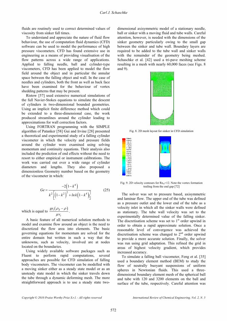
dimensional axisymmetric model of a stationary needle, ball or sinker with a moving fluid and tube walls. Careful attention, however, is needed with the dimensions of the sinker geometry particularly owing to the small gap between the sinker and tube wall. Boundary layers are required to be added to the tube wall and sinker walls with the remainder of the geometry being meshed. Schaschke et al. [42] used a tri-pave meshing scheme resulting in a mesh with nearly 60,000 faces (see Figs. 8 and 9).

Fig. 8. 2D mesh layout for sinker in CFD simulation

Fig. 9. 2D velocity contours for Rem=12. Note the vortex formation trailing from the end gap [72]

The solver was set to pressure based, axisymmetric

and laminar flow. The upper end of the tube was defined as a pressure outlet and the lower end of the tube as a velocity inlet in which all the sinker walls were defined as stationary. The tube wall velocity was set to the experimentally determined value of the falling sinker. The discretisation scheme was set to 1st order upwind in order to obtain a rapid approximate solution. Once a reasonable level of convergence was achieved the discretisation scheme was changed to 2nd order upwind to provide a more accurate solution. Finally, the solver was run using grid adaptation. This refined the grid in areas of highest velocity gradient, which provides increased accuracy.

To simulate a falling ball viscometer, Feng et al. [35] used a boundary element method (BEM) to study the flow of neutrally buoyant suspensions of uniform spheres in Newtonian fluids. This used a three-dimensional boundary element mesh of the spherical ball and tube with 120 and 3200 elements on the ball and surface of the tube, respectively. Careful attention was

Carl J. Schaschke


573

paid to applying the no-slip conditions on the surfaces of the tube and ball. The simulations involved permitting the ball to fall from rest to the bottom of the tube and the results were found to compare favourable with the analysis of Tanner [34] and prediction of Graham et al. [59].

The descending sinker was simulated for the range of isostatic pressures considered experimentally using available fluid property data for density and viscosity. The results of the simulations illustrated that a high level of vortex formation exists, which decreases with pressure and thus modified Reynolds number.

Schaschke et al. [42] found that the hemi-spherical or round-nosed sinker provided a channeling of flow into the annulus between the sinker and tube. The short entry length to form fully developed laminar flow was evident. From the tail-end, vortex formation was found to exist and was particularly evident at high sinker fall rates (see Figs. 10 and 11).

Fig. 10. 3D mesh for a falling sinker [72]

Fig. 11. Velocity vector for 3D CFD simulation. Rem=6.8 [72] The design of a sinker which avoids the complex flow

formations is complicated by the practicality of machining and fabrication. The CFD simulation supports the use of the sinker used but reliance on analytical solutions for flow must therefore be treated with caution. Calibration fluids therefore remain essential in order to provide the necessary accuracy with determined viscosity data.

XI. Models The viscosity of liquids can be obtained from direct

measurement of sinker fall times. As previously noted, the determinations are also dependent on accurate measurement of the sinker and tube dimensions as well

as the density data at elevated pressure. The viscosity of complex liquids such as polymers

and diesel fuels is well known to increase with decreasing temperature as well as increasing pressure. While there are many approaches to the evaluation of viscosity with temperature for complex liquids comparatively few are associated with the effects of pressure and even fewer when combined with temperature.

The viscosity of liquids under the influence of high isostatic pressure rises following the rather general rule in that the more complex the molecular structure of the liquid, the larger the effect of pressure. Simple quadratic or higher polynomial equations can also be used to relate viscosity to pressure over moderate pressure ranges.

A number of empirical expressions have been proposed relating viscosity to pressure. Based on the concept of free volume, the molecules are assumed to occupy a volume [60]-[62]. For isothermal conditions, the concept of free volume leads to the so-called Barus equation in which the viscosity is given by: ( )O exp pµ µ α= (26)

This has been used successfully to provide viscosity data with pressure from many applications. An example is shown in Fig. 12 and Table I.

0

0.5

1

1.5

2

2.5

3

3.5

4

4.5

5

0 20 40 60 80 100 120 140 160 180 200

Pressure (MPa)

Viscosity (m

Pa.s)

Fig. 12. Variation of viscosity with pressure for n-hexane/n-dodecane at

5oC. ● n-hexane, ◙ 25% n-dodecane, ■ 50% n-dodecane, ▲75% n-dodecane, ◊100% n-dodecane [71]

TABLE I

BARUS EQUATION CONSTANTS FOR N-HEXANE AND N-DODECANE AT 5OC AND 20OC [71]

5oC 20oC n-hexane/ n-dodecane

ηo mPa.s

α MPa-1

R2 ηo mPa.s

α MPa-1

R2

100% hexane 0.353 0.0072 0.980 0.315 0.0062 0.985 25% n-dodecane

0.528 0.0068 0.993 0.429 0.0066 0.989

50% n-dodecane

0.692 0.0082 0.995 0.592 0.0073 0.981

75% n-dodecane

1.905 0.0098 0.995 0.945 0.0082 0.996

100% n-dodecane

1.774 0.0133 0.992 1.422 0.0097 0.977

Studying the effect of pressure on the viscosity of

lubricants in bearing analysis, Kottke et al. [40] applied

Carl J. Schaschke


574

the Barus equation to many experimental data of liquids subjected to high pressure in which it was noted that experimental data does not fully obey the equation and the use of more accurate models is therefore necessary as noted by Bair et al. [63].

The molecular architecture of complex mixtures such as diesel fuels has a profound effect on rheological properties [64]. Hydrocarbon liquids and, in particular, their mixtures such as those of diesel fuels are highly complex in composition. In general, the rheological properties of long chain molecules are more complex than short chain molecules, which in turn are more complex than simple “spherical” molecules. Highly branched molecules are more complex again as, too, are mixtures of short and long molecules [64]. The complexity arises from the need for greater free volume void space in which to move. The exponential increase is to be expected due to the increasing compression of the molecules with pressure inhibiting or restricting molecular movement.

Xuan et al., [65] presented a novel model for correlating the viscosity of Newtonian liquids at high pressure, and based on the activation model, which can simultaneously be influenced by both temperature and pressure. Based on Hu and Lui’s work [66] for compressibility, the final expression contains two adjustable parameters, which are determined by fitting with literature viscosity data.

There are a number of models which take into account the combined effects of temperature and pressure on the rheological properties of fluids [67]. Some are empirical functions of temperature and pressure, while others are based on the concept of free-volume. Martínez-Boaz et al. [68] presents a comprehensive review of high pressure-temperature-viscosity relationships of used motor oil and vacuum residue blends over a range of shear rates spanning 1 to 100 s-1.

While the viscosity of simple and small molecules may be modelled using simple models, the situation is complicated with long chain molecules such as polymers and oil mixtures. Yoshimura et al. [69] presents viscosity data for a series of amines up to 100 MPa and between 20oC and 80oC, with respect to chain length. This was based on the Vogel-Fulcher-Tamman representation, a rough hard-sphere scheme and the concept of free-volume, in which success is reported and concluded to be a function of intermolecular repulsive potential.

A focus for the high pressure work is the oil industry. With this in mind, Boned et al. [70] presented high pressure viscosity and density data of two synthetic hydrocarbon mixtures examined seven different models, applicable to hydrocarbon fluids. These were based on classical mixing laws, the self-referencing model, hard sphere theory, free volume and the Lohrenz-Bray-Clark correlation.

XII. Conclusion The falling body viscometer is an effective tool for

determining the viscosity of a range of fluids at high pressure. There is a good degree of reproducibility of experimental data now being published. While theoretically predicted viscosities from analytical solutions for flow differ from those obtained experimentally, the use of calibration fluids remains a necessity to correct determined values. Numerical deviations from theoretical values are due to sinker end effects with manifest themselves as complex flow patterns emanating from the annulus formed between the sinker and tube. The use of CFD simulation and imaging approaches reveals evidence of complex circulating flow patterns of the fluid exiting from the annular gap. These flow patterns are influenced by the isostatic pressure, which affects the rate of sinker descent and thus the determination of viscosity.

With the heightened interest in high-pressure viscosity measurement, many more fluids and, in particular, complex liquids such as foods, polymers and biodiesels are becoming the focus of attention and can all lead to improvements in our understanding of the rheological changes all of which occur during the high pressure processing.

References [1] J. C. Cheftel, Applications des hautes pressions en technologie

alimentaire, Actualités des Industries Alimentaire et Agro-Alimentaire, 108 (1991) 141-153.

[2] D. Knorr, High pressure processing for preservation modification and transformation of foods, High Pressure Research 22 (2002) 595-599.

[3] S. Lee, D. Tanaka, J. Kusaka, Y. Daisho, Effects of diesel fuel characteristics on spray and combustion in a diesel engine, JSAE Rev., 23 (2002) 407-414.

[4] R. Dunn, M. Bagby, Low Temperature Filterability Properties of Alternative Diesel Fuels from Vegetable Oils, JAOCS., 73 (2006) 1719-1728.

[5] D. R. Caudwell, J. P. M. Trusler, V. Vesovic, W. A. Wakeman, The viscosity and density of n-dodecane and n-octadecane at pressures up to 200 MPa and temperatures up to 473 K, Int. J. Thermophys., 25(5) (2004) 1339-1352.

[6] H. Kashiwagi, T. Makita, Viscosity of twelve hydrocarbon liquids in the temperature range 298-348 K at pressures up to 110 MPa, Int. J. Thermophys., 3(4) (1982) 289-305.

[7] R. F. Chang, M. R. Moldover, High-temperature high pressure oscillating tube densimeter, Rev. Sci. Instrum., 67(1) (1996) 251-256.

[8] A. Kumagai, Y. Kawase, C. Yokoyama, Falling capillary tube viscometer for liquids at high pressure, Rev. Sci. Instruments, 69(3) (1998) 1441-1445.

[9] L. Kulisiewicz, A. Delgado, High-pressure rheological measurement methods: A review, Appl. Rheol. 20:1 (2010) DOI 10.3933/ApplRheol-20-13018.

[10] B. Calvignac, Mise au point de méthodes de caractérisation de binaires en milieu supercritiques et modélisation des propriétés physiques et thermodynamiques mesurées, Ph.D. dissertation, Ecole Nationale Supérieure des Mines de Paris. 2009.

[11] E. Kiran, Y. L. Sen, High-pressure viscosity and density of n-alkanes, Int. J. Thermophys., 13(3) (1992) 411-442.

[12] J. F. Stalnaker, R. G. Hussey, Wall effects on cylinder drag at low Reynolds number, Phys Fluids, 22(4) (1979) 603-613.

Carl J. Schaschke


575

[13] G. G. Stokes, On the effects of the internal friction on the motion of pendulums, Trans. Cambridge Philos. Soc., 9 (1851) 8-106.

[14] M. Brizard, M. Megharfi, E. Mahe, C. Verdier, Design of a high precision falling-ball viscometer, Rev. Sci. Instrum., 76 (2005) 025109.

[15] T. Lommatzsch, M. Megharfi, E. Mahe, E. Devin, Conceptual study of an absolute falling-ball viscometer, Metrologia 38 (2001) 531-534.

[16] N. A. Park, T. F. Irvine, The falling needle viscometer: A new technique for viscosity measurements, Wärme- und Stoffübertragung 18 (1984) 201-206.

[17] N. D. Cristescu, B. P. Conrad, R. Tran-Son-Tay, A closed form solution for falling cylinder viscometers, Int J. Eng Sci. 40 (2002) 605-620.

[18] J. Lohrenz, An experimental verified theoretical study of the falling cylinder viscometer, Ph.D. dissertation, University of Kansas, Lawrence USA, 1960.

[19] J. Lohrenz, G. W. Swift, F. Kurata, An experimentally verified study of the falling cylinder viscometer, AIChE J. 6(4) (1960) 547-550.

[20] E. Ashore, R. B. Bird, J. A. Lesearboura, Falling cylinder viscometer for non-Newtonian fluids, AIChEJ., 11 (1965) 910-916.

[21] F. J. Eichstadt, G. W. Swift, Theoretical analysis of the falling cylinder viscometer for power law and bingham plastic fluids, AIChEJ., 12(6) (1966) 1179-1183.

[22] F. Ramsteiner, Falling cylinder viscometer for determination of the viscosity of polymer melts under hydrostatic pressure, Rheol. Acta., 15(7-8) (1976) 427-433).

[23] E. T. S. Huang, G. W. Swift, F. Kurata, Viscosity of methane and propane at low temperature and high pressure, AIChEJ. 12 (1966) 932-936.

[24] A. Dandridge, D. A. Jackson, Measurement of viscosity under pressure: a new method, J. Phys. D: Appl. Phys. 14(5) (1981) 829-831.

[25] S. Claesson, S. All, J. L. McAtee, New types of viscometer plummets for measuring viscosity of low viscosity liquids under pressure, Industrial & Chemistry Engineering, Process Design and Development 22(4) (1983) 633-635.

[26] E. G. Wehbeh, T. J. Ui, R. G. Hussey, End effects for the falling cylinder viscometer, Phys Fluids A 5(1) (1993) 25-33.

[27] M. C. S. Chen, J. A. Lescarboura, G. W. Swift, The effect of eccentricity on the terminal velocity of the cylinder in a falling cylinder viscositer, AIChEJ., 14(1) (1968) 123-127.

[28] F. Gui, T. F. Irving, Theoretical and experimental study of the falling cylinder viscometer, Int J. Heat Mass Transfer 37(1) (1994) 41-50.

[29] N. A. Park, T. F. Irvine, Measurement of rheological fluid properties with the falling needle viscometer, Rev. Sci. Instrum. 59(9) (1988) 2051-2058.

[30] N. A. Park, Y. I. Cho, T. F. Irvine, Steady shear viscosity measurements of viscoelastic fluids with the falling needle viscometer, J. Non-Newtonian Fluid Mech. 34 (1990) 351

[31] K. Cho, Y. I. Cho, N. A. Park, Hydrodynamics of a vertically falling thin cylinder in non-Newtonian fluids, J. Non-Newtonian Fluid Mech. 45 (1992) 105.

[32] R. Zheng, N. Phan-Thien, V. Ilic, Falling needle rheometry for general viscoelastic fluids, J. Fluid Eng. 116 (1994) 619.

[33] A. M. J. Davis, H. Brenner, The falling-needle viscometer, Physics of Fluids 13(10) (2001) 3086-3088.

[34] R. I. Tanner, End effects in falling-ball viscometry, J. Fluid Mech. 17 (1963) 161-170.

[35] S. Feng, A. L. Graham, P. T. Reardon, J. Abbott, L. Mondy, Improving falling ball tests for viscosity determination, J. Fluids Eng. 128 (2006) 157-163.

[36] E. R. Lindgren, Note on falling cylindrical-shell viscometer Rev. Sci Instrum. 43(3) (1972) 557-560.

[37] P. W. Bridgman, The effect of pressure on the viscosities of forty-three pure liquids, Proc. Am. Acad. Arts Sci. 61 (1926) 56.

[38] J. B. Irving, The effect of non vertical alignment on the performance of a falling-cylinder viscometer, J. Physics. D: Appl. Phys. 5 (1972) 214-224.

[39] C. J. Schaschke, S. Allio, E. Holmberg, Viscosity measurement of vegetable oil at high pressure, Trans IChemE 84(C) (2006) 173-178.

[40] P. A. Kottke, S. S. Bair, W. O. Winer, The measurement of viscosity of liquids under tension, J. Tribology 125 (2003) 260-265.

[41] J. H. Dymond, K. J. Young, J. D. Isdale, Transport properties on nonelectrolyte liquid mixtures, Int. J. Thermophysics 1(4) (1980) 345-373.

[42] C. J. Schaschke, S. Abid, I. Fletcher, M. J. Heslop, Evaluation of a falling sinker-type viscometer at high pressure using edible oil, J. Food Eng., 87 (2008) 51-58.

[43] J. B. Irving, A. J. Barlow, An automatic high pressure viscometer, J. Physics 4 (1971) 232-236.

[44] N. A. Park, T. F. Irvine, Falling cylinder viscometer end correction factor, Rev Sci. Instrum. 66(7) (1995) 3982-3984.

[45] S. C. Vant, Investigation of fluid properties at non-ambient conditions, Ph.D. dissertation, Dept Chem. Proc. Eng., University of Strathclyde, Glasgow, UK, 2002.

[46] A. Baylaucq, M. J. P. Comuñus, C. Boned, A. Allal, J. Fernández, High pressure viscosity and density modeling of two polyethers and two dialyl carbonates, Fluid Phase Equilibria, 199 (2002) 249-263.

[47] B. I. Lee, M. G. A. Kesler, A Generalized Thermodynamic Correlation Based on Three-Parameter Corresponding States, AICheEJ. 21 (1975) 510-527.

[48] J. H. Dymond, R. Malhotra, Densities of n-alkances and their mixtures at elevated pressures, Int. J. Thermophys., 8(5) (1987) 541-555.

[49] J. H. Dymond, R. Malhotra, The Tait equation: 100 years on, Int. J. Thermophysics, 9(6) (1988) 941-950.

[50] J. H. Dymond, J. Robertson, J. D. Isdale, (p, ρ, T) of some pure n-alkane and binary mixtures of n-alkanes in the range 298-373 K and 0.1 to 500 MPa, J. Chem. Thermodynamics 14 (1982) 51-59.

[51] V. N. Belonenko, V. M. Troitsky, Y. E. Belyaev, J. H. Dymond, N. F. Glen, Application of a micro-pVT apparatus for the measurement of liquid densities at pressures up to 500 MPa, J. Chem. Thermodynamics., 32 (2000) 1203-1219.

[52] S. R. Reid, C. Peng, N. A. Park, T. F. Irvine, Liquid density measurements using the falling needle viscometer, Int. Commun. Heat Mass Transfer 24(3) (1997) 303-312.

[53] K. R. Harris, L. A. Woolf, M. Kanakubo, Temperature and pressure dependence of the viscosity of the ionic liquid 1-buyl-3-methylimidazolium hexafluorophosphate, J. Chem. Eng Data, 50 (2005) 1777-1782.

[54] K. R. Harris, M. Kanakubo, L. A. Woolf, Temperature and pressure dependence of the viscosity of the ionic liquids 1-hexyl-3-octylimidazolium hexafluorophosphate and 1-methyl-3-octylimidazolium tetrafluorophosphate, J. Chem. Eng Data, 51 (2006) 1161-1167.

[55] K. R. Harris, M. Kanakubo, L. A. Woolf, Temperature and pressure dependence of the viscosity of the ionic liquids 1-hexyl-3-methylimidazolium hexafluorophosphate and 1-butyl-3-methylimidazolium bis(trifluoromethylsulfonyl)imide, J. Chem. Eng. Data 52 (2007) 1080-1085.

[56] Z. Minyu, C. J. Schaschke, High Pressure Falling Sinker Liquid Viscosity Determination Without Supplementary Density Data: A New Approach, Int J Chem Eng. (2009) Doi 10.1155/2009/747592.

[57] G. H. Ristow, Wall correction for sinking cylinders in fluids, Physical Rev. 55(3) (1997) 2808-2813.

[58] S. V. Patanker, Numerical Heat Transfer and Fluid Flow. McGraw-Hill. New York, USA (1980).

[59] A. L. Graham, L. A. Moody, D. J. Miller, N. J. Wagner, W. A. Cook, Numerical solutions of eccentricity and end effects in falling ball rheometry, J. Rheol. 33(7) (1989) 1107-1128.

[60] R. C. Reid, J. M. Prausnitz, B. E. Poling, In The properties of gases and liquids, (4th edition, McGraw-Hill Book Company, New York, 1987, 314-332).

[61] M. M. Aalto, K. I. Keskinen, Liquid densities at high pressure, Fluid Phase Equilibria 166 (1999) 183-205.

Carl J. Schaschke


576

[62] A. Allal, M. Moha-Ouchane, C. Boned, A new free volume model for dynamic viscosity and density of dense fluids versus pressure and temperature, Phys. Chem. Liq. 39 (2001), 1-30.

[63] S. Bair, J. Jarzynski, W. Winer, The temperature, pressure and time dependence of lubricant viscosity, Tribol. Int. 34 (2001) 461-468.

[64] K. I. Kioupis, E. J. Maginn, Impact of Molecular Architecture on the High-Pressure Rheology of Hydrocarbon Fluids, J. Phys. Chem. B, 104 (2000) 7774-7783.

[65] A. Xuan, Y. Wu, C. Peng, P. Ma, Correlation of the viscosity of pure liquids at high pressure based on an equation of state, Fluid Phase Equilibria 240 (2006) 15-21.

[66] Y. Hu, H. L. Liu, J. M. Prausnitz, Equation of state for fluids containing chain-like molecules, J. Chem. Phys. 104 (1996) 396.

[67] J. Lamb, Viscoelasticity and lubrication: a review of liquid properties, J. Rheol. 22(4) (1978) 317.

[68] F. Martínez-Boaz, F. Fernandez-Latorre, C. Gallegos, High-pressure viscosity of used motor oil/vacuum residue blends, Fuel 88 (2009) 1595-1601.

[69] M. Yoshimura, C. Boned, A. Balaucq, G. Galliéro, H. Ushiki, Influence of the chain length on the dynamic viscosity at high pressure of some amines: Measurement and comparative study of some models, J. Chem. Thermodyn. 41 (2009) 291-300.

[70] C. Boned, C. K. Zéberg-Mikkelsen, A. Baylaucq, P. Dauge, High-pressure viscosity and density of two synthetic hydrocarbon mixtures representative of some heavy petroleum cuts, Fluid Phase Equilibria 212 (2003) 143-164.

[71] E. P. Fernandez, C. J. Schaschke, Viscosity measurement of n-dodecane and n-hexane and their binary mixtures at combined high pressure and ambient and sub-ambient temperatures of 20oC and 5oC, Int. Rev. Chem. Eng. 2(3) (2010) 364-370.

[72] S. Saied, Evaluation of a falling body-type viscometer at high pressure. Ph.D. dissertation, Dept Chem. Proc. Eng., University of Strathclyde, Glasgow, UK, 2009.

Author’s information Department of Chemical & Process Engineering, University of Strathclyde, 75 Montrose Street, Glasgow, UK.

Carl J Schaschke gained his PhD in Chemical Engineering from the University of Strathclyde in 1990. He is professor and has been head of the department of Chemical & Process Engineering at Strathclyde since 2006. He is a Fellow of the Institution of Chemical Engineers and a member of the European Federation of Chemical Engineers (EFCE) Working Party on

High Pressure Technology. He works of fluid measurement across a diverse range of industries from oil and gas to honey processing.

high pressure viscosity measurement with falling body … pressure viscosity measurement... · the...

Documents