high resolution geoacoustic inversion in shallow water: a

SACLANTCEN MEMORANDUM . serial no.: SM-361

RESEARCH CENTRE MEMORANDUM

C. W. Holland, J.. Osler

December 1998

' . . . : . - I , ,. . , .

' - 1 ' . I t I. ' I

i , , , I . . ,

Report no. changed (Mar 2006): SM-361-UU

This document is approved for public release. Distribution is unlimited

SACLANT Undersea Research Centre Viale San Bartolomeo 400 19138 San Bartolomeo (SP), Italy

tel: +39-0187-540.111 fax: +39-0187-524.600

e-mail: [email protected]

NORTH ATLANTIC TREATY ORGANIZATION


SACLANTCEN SM-36 1

High resolution inversion in shallow water: a joint time and frequency domain technique

Charles W. Holland, John Osler

The content of this document pertains to work performed under Project 042- 1 of the SACLANTCEN Programme of Work. The document has been approved for release by The Director, SACLANTCEN.

Jan L. Spoelstra Director


SACLANTCEN SM-36 1

intentionally blank page


SACLANTCEN SM-361

High resolution geoacoustic inversion in shallow water: a joint time and frequency domain technique

Holland, C.W., Osler, J.

Executive Summary: Sonar system performance in shallow water is often constrained by interaction with the seafloor. The accuracy of performance predictions is generally limited by knowledge of the seafloor properties rather than model physics. Therefore there is a need for methods by which the seafloor properties, or geoacoustic data, can be estimated. Our application for the geoacoustic data requires high spatial resolution because we require the geoacoustics for both propagation and reverberation. Since direct measurement of geoacoustic data is difficult, time-consuming and expensive, inversion of acoustic data is a promising alternative. However, the main problem encountered in geoacoustic inversion is the problem of uniqueness, i.e., many diverse geoacoustic models can be made to fit the same data set. A second problem encountered in geoacoustic inversion is that the resulting properties are generally low resolution in the sense of that seafloor properties are averaged over many kilometres. In order to meet the stringent requirements of high spatial resolution and uniqueness, an entire method has been developed including a new measurement technique, processing/analysis technique, and inversion strategy. The inversion strategy is based on a novel combination of a time domain inversion and frequency domain extraction. In this report we describe each of these techniques and then show how they were applied to measurements at a shallow water site in the Mediterranean Sea.


SACLANTCEN SM-361

intentionally blank page


SACLANTCEN SM-361

High resolution geoacoustic inversion in shallow water: a joint time and frequency domain technique


Abstract: High resolution geoacoustic data are quired for accurate predictions of acoustic propagation and scattering in shallow water. Since direct measurement of geoacoustic data is difficult, time-consuming and expensive, inversion of acoustic data is a promising alternative. However, the main problem encountered in geoacoustic inversion is the problem of uniqueness, i.e., many diverse geoacoustic models can be made to fit the same data set. A key, and perhaps unique, aspect of this approach is the combination of data analysis in both the space-time and the space-fkquency domains. This combination attempts to ameliorate the uniqueness problem by incorporating as much independent data as possible in the analysis. In order to meet the stringent requirements of high spatial resolution and uniqueness, an entire method has been developed including a new measurement technique, processing/analysis technique, and inversion strategy. In this paper we describe each of these techniques and then show how they were applied to a shallow water data set in the Mediterranean Sea. The resulting sound speed @en& in the upper 150 m sub-bottom appear to be much higher (one order of magnitude) than generally assumed. Inversion results in the upper several meters compare favorably with axe analysis.

Keywords: geoacoustic inversion, shallow water, sediment layering, bottom reflection, sediment sound speed merits


SACLANTCEN SM-36 1

Contents

............................................................................................................ 1 Introduction 1

2 . Experiment design ................................................................................................. 3

2.1. Source .............................................................................................................. 4

2.2. Receiver ........................................................................................................... 5

3 . Data processing ....................................................................................................... 6

3.1 . Time domain .................................................................................................... 6

..................................................................... 3.2. Frequency domain - bottom loss 6

....................................................................... . 4 Modelling, extraction and inversion 9

..................................................................... 4.1. Time domain - inversion method 9 ............................................................ 4.2.Time domain - synthetic seismograms 11

4.3. Frequency domain ...................................................................................... I I

............................................................................................. 5 . Discussion of results 13

5.1 . Time domain - Bryan method .................................................................... 1 3

......................................................................................... 5.2. Frequency domain 14

5.3. Time domain synthetics ................................................................................. I7

5.4. Ground truthing ............................................................................................. 19 6 . Summary ............................................................................................................... 21

References ................................................................................................................. 22

Annex A .................................................................................................................... 23


SACLANTCEN SM-36 1

Introduction

Shallow water' acoustic propagation is often constrained by interaction with the seafloor. Prediction accuracy is generally limited by knowledge of the seafloor properties rather than model physics. Therefore there is a need for methods by which the seafloor properties can be estimated. A simplified description of the seafloor properties that controls seafloor interaction over a particular frequency band of interest is called a geoacoustic model. The model includes compressional2 speed, density, and attenuation as a function of depth and the latter as a function of frequency.

Our application for the geoacoustic model requires high spatial resolution since we require the geoacoustics for both propagation and scattering3 or reverberation. This concept of a self-consistent geoacoustic model, i.e., a model capable of treating both the propagation and the scattering with the same physical descriptors, is different from the common approach of treating the propagation with a geoacoustic model and the scattering with an empirical scattering kernel. The concept of a self-consistent geoacoustic model was explored in a deep-water environment in Holland and Neumann (1998). In this paper the problem of high resolution geoacoustic inversion is addressed. In a later study the application of these data to propagation and scattering will be examined.

Since direct measurement of geoacoustic data is difficult, time-consuming and expensive, inversion of acoustic data is a promising alternative. However, the main problem encountered in geoacoustic inversion is the problem of uniqueness, i.e., many diverse geoacoustic models can be made to fit the same data set. For some applications this does not pose a serious problem since only a parameterization that fits the data is required without a requirement that the parameters represent actual physical properties. However, for our application, the sediment physical properties, not just parameters are required. One way to improve uniqueness, i.e., improve the likelihood of obtaining properties and not geo-parameters, is to employ more (independent) data. For example, one approach that has been widely used is to employ data over a broad frequency band (e.g., Gerstoft and Gingras (1996)). In this method we attempt to use as much independent data as possible over three domains: time, frequency, and space.

I By shallow water we generally mean continental shelf regions, however, i t can mean by extension any Ft tom limited region. - The inversion technique is capable of including shear waves. However, for the environment examined in this paper shear waves contributed negligibly and thus are not included in the geoacoustic model.

The scattering from sub-bottom sediment volume inhomogeneities requires substantially higher resolution in the geoacoustics than does the propagation.


SACLANTCEN SM-36 1

based on a novel combination of a time domain inversion and frequency domain extraction. The time domain inversion uses the wide angle reflection data to obtain layer thicknesses and interval velocities; this step solves a second problem in geoacoustic inversion which is to adequately define the initial parameterization (e.g., how many layers should be considered in the solution space). The reflectivity (or bottom loss) analysis in the frequency domain provides attenuation as a function of depth and frequency and density as a function of depth. A new analysis technique exploits cumulative time windowing of the bottom loss to improve resolution in depth for the density and attenuation estimates.

In order to meet the stringent requirements of high spatial resolution and uniqueness, an entire method has been developed including a new measurement technique, processing/analysis technique, and inversion strategy. In this paper we describe each of these techniques and then show how they were applied. Details of the experiment design and processing are provided in Sections 2 and 3. Section 4 describes the inversion and modelling procedures and Section 5 provides discussion of the results at a shallow water site in the Mediterranean Sea.


SACLANTCEN SM-36 1

Experiment design

A common method of geoacoustic inversion in shallow water is to employ propagation data over spatial scales of kilometres or tens of kilometres; the resulting data therefore represent a spatial average over a large measurement aperture. The requirement for high regional range resolution in our approach was met by using the strategy of making multiple very short aperture (termed 'local') measurements, with spatial averaging over scales of a few hundred meters. In addition to the advantage of a smaller spatial averaging footprint, the local measurements have the additional advantage of being less sensitive to oceanographic variability that sometimes plagues shallow water geoacoustic inversion. Interpolation between 'local' measurements using seismic reflection data has the potential for a regional range dependent model with high resolution. In this paper we address the local measurement and inversion problem.

The requirement for high resolution in depth suggests that the source pulse length should be short (which also fits the requirement of obtaining data over a broad bandwidth) with dense along-track sampling. A Uniboom source was selected because it transmits a short repeatable pulse at high repetition rates. A sparker source was also examined but later discarded because the pulse was neither repeatable nor sufficiently short.

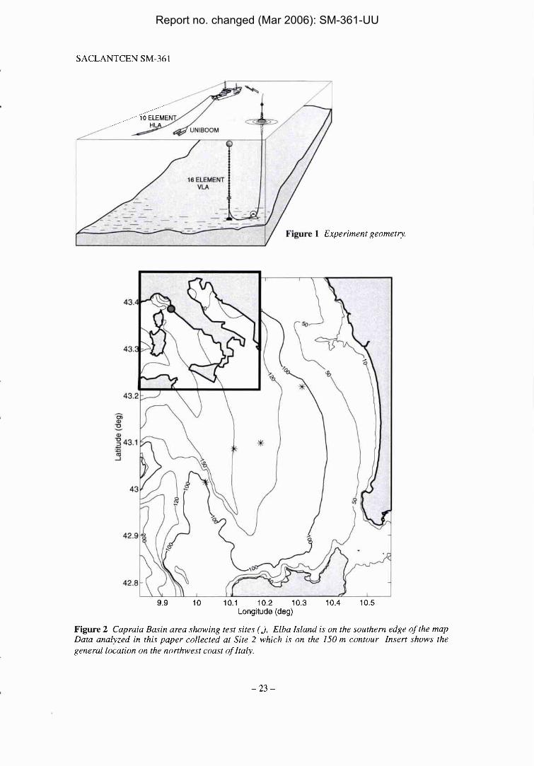
The experiment geometry as shown in Fig. 1 consists of the towed Uniboom source and a bottom moored receiver. This measurement technique has been conducted at several sites in the northern Tyrrhenian Sea as shown in Fig. 2. In this case a 16 element vertical line array (VLA) was employed although the analysis here uses data from one hydrophone. After deployment, the VLA geographic position was fixed within an estimated rms error of less than 8.5 m using transponders on the huli and bottom of the VLA.

The acoustic data were collected along orthogonal tracks with the center intended to be directly over the array position. This pattern allows data to be acquired over a wide range of grazing angles in four azimuths around the array. The length of each leg is determined based upon the local sound speed profile, water depth and array depth, but a typical spatial aperture of the measurement is of order 1 km. The close proximity of the ship to the array required gas turbines to be used in order to minimize contamination from own-ship noise. DGPS was employed for navigation and timing. Supporting environmental data included seismic reflection profiling, CTDlXBTs, bathymetry, gravity and piston cores, and side scan data.


SACLANTCEN SM-361

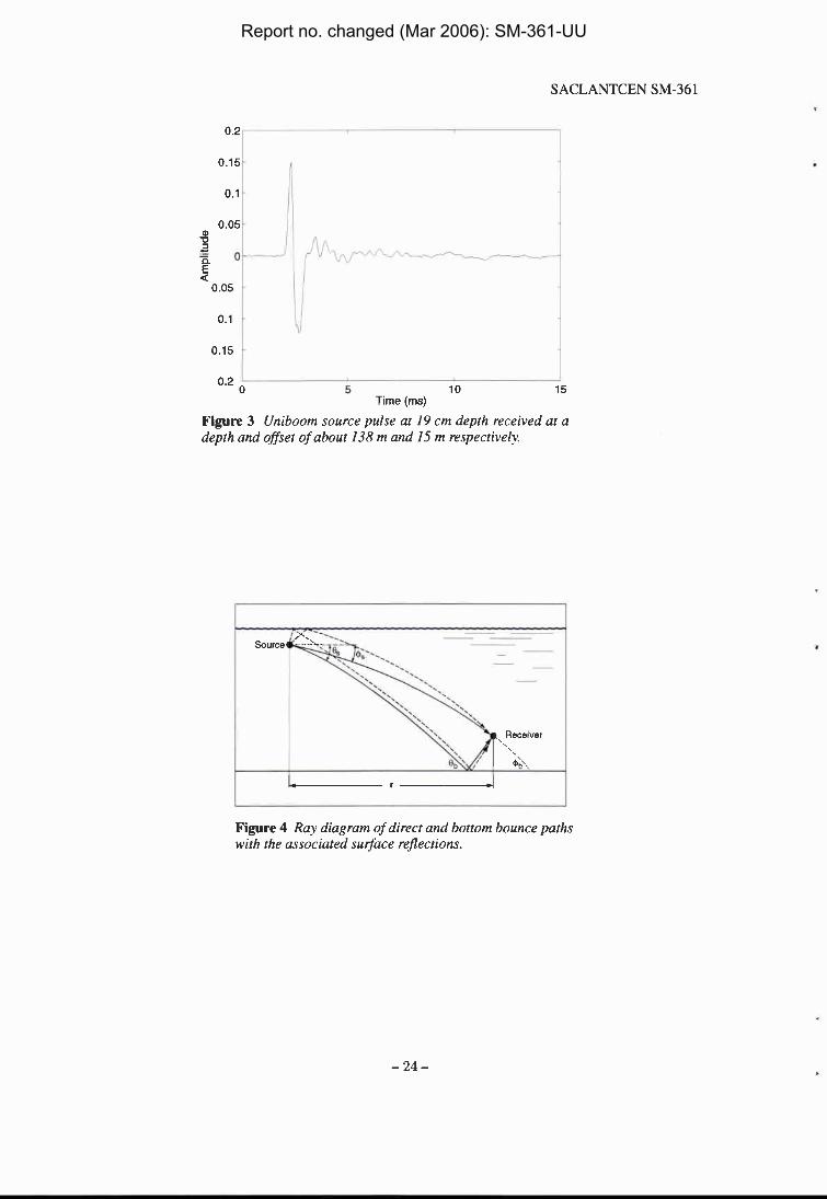
2.1. Source The source was an EG&G model 265 Uniboom which had desirable qualities of a repeatable short pulse length and broad bandwidth (600-6000 Hz). Its electromechanical assembly consists of an insulated round metal plate of radius 0.2 m and rubber diaphragm adjacent to a flat-wound electrical coil. A short duration high energy (300 J) electrical pulse discharges into the coil and the resultant magnetic field explosively repels the metal plate. The plate motion in the water generates a single broadband acoustic pressure pulse less than 1 ms in duration (see Fig. 3) with a broadband source level of 207 dB re 1 pPa. The source was mounted on a catamaran with a source depth of about 0.2 m and tow speed of 4 kn. The pulse repetition rate was 15 pulses per minute or 1 pulse approximately every 8 meters. This repetition rate yielded a high data density for the measured wide angle reflection seismogram and an excellent resolution in grazing angle for the bottom loss data. Uniboom pulses are initiated by a trigger controlled from a GPS clock. The data acquisition is also keyed to GPS, which avoids the tedious and error prone task of clock synchronization.

The difficulty in using the Uniboom as opposed to more conventional sources is that the source plate characteristics were not known. Also the catamaran has a slight, but unknown, tilt. The source characteristics were estimated by using the direct path arrival on the vertical array. Figure 4 shows a ray diagram of the experiment including the direct and bottom reflected paths. The source beampattern and presence of the image path eliminates the possibility of performing a self-calibrating technique. Instead we use the direct path to extract source level as follows:

Where TL,, and RL,, are the theoretical transmission loss and measured received level for the direct path (including the surface image) over a 113 octave bandwidth. TL,,, is computed using two rays coherently summed then frequency averaged.

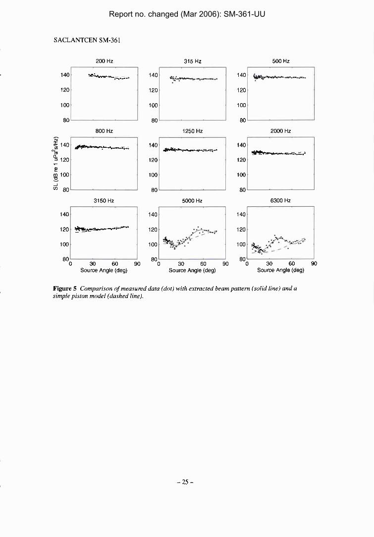
Figure 5 shows a comparison of the measured source level for an integration time4 of 15 ms with a model based on the classical radiation from a plane, circular, baffled, piston. These model results are shown only to demonstrate that they capture the general characteristics of the source. The details of the data are not well-modelled because model assumptions are not met, most notably the assumption of an infinite baffle. Because of the complexity of the source, the mount, and the sled, our approach to source modelling was to simply fit a polynomial to the measured data. This fit is done for each leg since the sled tilt is different depending on whether the leg is approaching or receding from the array.

The low frequency ringing of the transducer following the electrical discharge is small (see Fig. 3) but not negligible. The source ringing has two undesirable effects. First, it places a lower limit on the receiver height above the seafloor (a receiver close to the seafloor may be contaminated by the extended source pulse depending on the magnitude of the bottom reflectivity). Second, the source level is a function of integration time

" Integration times vary depending upon source-receiver offset. All integration times are given referenced to the value at normal incidence.


SACLANTCEN SM-36 1

which places limits on the bottom loss integration times. Figure 6 shows the dependence of the source level (direct path) received level on integration time. The data have been normalized to the longest integration time of 48 ms. For data above 1000 Hz, the source level appears to be independent of integration time for times greater than 6 ms. For longer integration times, lower frequencies can be used. For the data shown in this paper, 630 Hz was the lowest frequency analyzed.

2.2. Receiver The receiver consisted of 16 Benthos AQ-4 hydrophones spaced irregularly over a 62 m aperture. The data were sampled at 24 kHz and low pass filtered at 8 kHz with a seven- pole six-zero elliptic (70 dB per octave roll off) anti-alias filter. The variable RC high pass filter (6 dB per octave roll off) was set at 150 Hz. A high speed digital link within the array provided programmable signal conditioning, digitization and serialization of the signals. Non acoustic data (gains, filter settings, etc..) were interleaved in the serial stream and telemetered to the NATO Research Vessel Alliance. The system filter and gain settings (0-84 dB in 6 dB steps) are user-programmable via telemetry.

The limited dynamic range of the VLA (about 60 dB) meant that gains had to be manually changed frequently near the VLA. Also, the close approach to the VLA meant that the RF antennae had to be manually steered resulting in some data drop-outs. Nevertheless, the overall quality of the data was very high.


SACLANTCEN SM-36 1

Data Processing

In this section the processing of the data in the time and frequency domains is discussed. One of the assumptions in the processing and analysis is that the environment can be approximated as range independent. The short spatial aperture over which the measurements are conducted makes this assumption valid for environments that we have investigated. For example at Site 2 where the maximum offset (horizontal source - receiver separation) was 800 m, acoustic interaction with the seafloor interface occurs within 100 m of the array for the bottom phone. Interaction with sub-bottom layers spans a somewhat larger offset of approximately 300 m (depending on the sub-bottom sound speed structure). Seismic reflection data indicate that the range independent assumption is justified over these range scales.

3.1. Time domain Quality control checks are applied to the time domain data, including the removal of seismograms which are contaminated by RF or other spurious noise and ensuring that array gain changes have been properly logged and applied to the data. Seismograms which are clipped, usually on the direct arrival, are removed from the bottom loss analysis. However, they are not removed from the time domain analysis as the clipping has little effect, with the possible exception of comparison of synthetic and data.

Horizontal source-receiver offsets are calculated using time of flight of the direct arrival, the experimental geometry (source, receiver, and water depths), and an eigenray model (Westwood and Vidmar, 1987) using the measured sound velocity profile. Initial attempts to construct seismograms using horizontal source-receiver offsets based on the DGPS position of the Alliance and the array position failed due to insufficient accuracy. In addition, the assumption of straight line ray paths (an isovelocity water column) was found to be inappropriate for our measured sound velocity profiles, in particular for the shallower grazing angles.

3.2. Frequency domain - bottom loss Bottom loss has historically been primarily a deep water measurement. In shallow water the short intervals between multipaths make separation of the bottom arrivals difficult. In our experiment geometry, the separation of multipaths is possible because of the very shallow tow depth (the surface and non-surface reflected path have nearly the same


SACLANTCEN SM-36 1

characteristics) the short duration of the transmit pulse, and the relatively short measurement aperture.

Bottom loss as a function of frequency, f, and specular angle, 4, at the water-sediment interface and integration time T can be calculated from a simple sonar equation as:

where TLP,, is the theoretical transmission loss from a perfectly reflecting bottom, RLhh is the measured received level in one-third octave bands associated with the bottom interacting arrival and SLF is the fitted source level from Eq. 1 at angles corresponding to the bottom bounce path. A signal-to-noise criteria of 6 dB was used both for the individual data points and a fitted curve.

Traditionally, bottom loss has been processed as a total energy quantity, i.e., integrated over all bottom arrivals. However, this method generally leads to severe uniqueness problems inasmuch as there can be many diverse parameter sets that explain the data equally well. In order to hone in on the 'true' solution, the bottom loss data are processed for selected cumulative time (or equivalently sub-bottom depth) intervals q: first across just the water-sediment interface, then across the water-sediment interface plus the next layer, and continuing until all layers are included in the integration. In the inversion, the geoacoustics are first extracted starting from the BL data at the water-sediment interface. Then those properties are fixed and the next BL data set including the next horizon are analyzed, and so forth until the last data set which is integrated over all arrivals. In this way the gradients in velocity, density and attenuation can be better constrained. The cumulative approach also has the advantage of indicating sensitivity of the BL to deeper layers. Data windowing is limited, of course, by the pulse length and the relative interval velocity between adjacent layers. In practice the time windows are placed between layers or layer groups in such a way that there is no danger of cutting across layer boundaries.

Frequently, bottom loss data are smoothed over some range of angles as an attempt to reduce 'random' scatter arising from imprecise knowledge of the geometry and environment. However, in order to maximize resolution in angle space, no smoothing is done in our processing. In other words, there is information in the angular dependence that can be useful for geoacoustic inversion. If the measurement and processing are performed with sufficient care, it appears possible to avoid angle smoothing altogether.

Standard bottom loss processing (e.g., Eq. 2) makes the implicit assumption that the bottom is a halfspace since the correction for the transmission loss in the water is applied only to the sediment reflected path at 8,. When sub-bottom paths contribute as in Fig. 7, the measurement represents a non plane-wave bottom loss. That is, the measurement includes energy from multiple angles. The presence of sub-bottom paths leads to artifacts in the data including the infamous "negative bottom loss" anomaly. Thus, it is possible in processing such as Eq. 2 to arrive at the wholly undesirable result of different bottom loss values depending upon source-receiver geometry. Using a source with a


SACLANTCEN SM-36 1

beam pattern further complicates matters. In the case of the Uniboom it means that at moderate5 frequencies, the beam pattern is corrected only at the angle of the sediment reflected path, and not for any other sub-bottom paths (even though the loss may be dominated by the sub-bottom paths).

These problems (relating to the incorrect halfspace assumption) can be addressed either in the data processing stage or in the modelling stage. For purposes here, it is more convenient to treat these problems in the modelling and retain simplicity in the data processing.

' At low frequencies the Uniboom is omnidirectional and at high frequencies the sub-bottom paths contribute negligibly because of attenuation.


SACLANTCEN SM-36 1

Modelling, extraction and inversion

The objective of the inversion and extraction techniques is to recover the deterministic sediment geoacoustic properties. A unique aspect is the coordinated analysis of data in both the time-space and frequency-space domains. The analyses performed in each domain are not necessarily new, but their combination is new (according to the authors' knowledge). Our technique attempts to use as much independent data as possible (across time, frequency, and space) and to extract information from each data type that is most suitable. For example, sound speed information is best extracted from the time domain, whereas, attenuation is best extracted from the frequency domain.

The first step in the technique is to use the time domain data to invert for the interval velocity and thickness of each layer. This provides the crucial initial parameterization, in terms of identifying the number of layers and provides an important advantage over many geoacoustic inversion techniques that have no basis for selecting the number of layers on which to perform the inversion. The second major step is to use the frequency domain data (bottom loss) to extract density and attenuation, as well as to refine the velocity structure. Finally, the geoacoustic properties are refined by alternating between the synthetic seismogram analysis and the bottom loss analysis.

4.1 Time domain - inversion method Assuming that the velocity structure above a given layer is a function of depth only, Dix (1955) showed that it is possible to determine the velocity and thickness of a homogeneous layer embedded in an arbitrary sequence of layers, without prior knowledge of the overlying structure. The interval velocity, v,, , of a layer is determined

from the root mean square velocities of the wide angle reflections from the top, v ~ ~ ~ _ ~ ,

and bottom, vRMsn, interfaces of the layer,

The root mean square velocity is defined as


SACLANTCEN SM-361

with t, being the zero-offset travel time within a layer. Le Pichon et al. (1968) incorporated the Dix method to calculate an initial velocity structure of deep-sea sediments in their technique that used conventional sonobuoys deployed while the vessel was underway conducting seismic reflection profiling. This velocity structure was then revised by iterative forward modelling to improve the fit between measured and modelled travel times, progressing from shallower to deeper layers. Implicit in this technique is the assumption that the velocity structure may be treated as a sequence of isovelocity layers, including the water layer, thus assuming straight line ray paths segments in each layer.

As documented by Bryan (1974, 1980), the application of straight-line paths to layers which are not homogeneous leads to errors which may be significant in certain cases. In particular, errors in the water column which are negligible in comparison with the times and offsets involved in the water column can be appreciable as the error is magnified as a sub-seabed layer gets thinner. In the absence of a detailed water velocity structure to overcome the assumption of straight line ray paths, the method of Le Pichon et al. is limited to water depthllayer thickness ratios of up to about 15 (Bryan, 1974).

Bryan (1974, 1980) presented an alternative approach, the ray-parameter method (see annex), which he used for characterizing relatively thin layers near the sea floor in deep water. His experimental data involved both the source and receiver located on the seabed, an optimal configuration from the standpoint of avoiding lateral variations in the water column. However, the theory is more general and allows for diverse experimental geometries such as the surface towed source and bottom moored receiver as used in our experiments. Since this method allows the resolution of thinner layers and is valid over a wider range of incident angles, it is a suitable choice for the inversion of wide-angle reflection data in shallow water.

The implementation of the Bryan inversion method involves fitting an hyperbola to each of the wide angle reflections which determines the zero-offset travel time and stacking velocity, t', and vzST (see annex for details on the theory). The hyperbola fitting is done interactively with a visual display of data, presented as a reduced travel time (t2 - x2 1 v2,, where v, is the reducing velocity generally chosen to be the depth averaged sound speed in the water column) versus offset plot. Hyperbolae were fitted qualitatively, i.e., "by eye". Once the hyperbolae have been defined, the layer thicknesses and interval velocities are immediately computed from Eq. A3.

Interval velocities recovered from the Bryan method are averaged both on a micro and macro scale. That is, there are fine-scale fluctuations in the velocity structure within a layer as well as larger scale variability, e.g. velocity gradients. The small scale velocity fluctuations are not addressed in this paper. Velocity gradients are extracted at a later point in the analysis.


SACLANTCEN SM-36 1

4.2 Time domain - synthetic seismograms The objective for the synthetic seismograms was to 1) aid in interpreting the measured data 2) guide the time domain pick criteria, and 3) refine the geoacoustic model. The generation of the synthetic seismograms follows Westwood and Vidmar (1987). It uses the same ray-based approach as in the bottom loss modelling (see next section), except that no attempt is made to correct for the source beampattern. The receiver response for individual eigenrays (see the first term in Eq. 4) are calculated then summed with the proper delay based on the travel times. An approximate source function was employed using the source data of Fig. 3 with the surface reflection removed. The sampling frequency in the synthetics is 16384 Hz, with a bandpass filter of 800-7000 Hz and Hamming window roll-offs of 400 Hz below and above the band.

In an isovelocity water column the direct and bottom bounce arrivals would appear as straight lines in reduced time. Synthetics allowed us to examine the isovelocity approximation and determine that the isovelocity approximation for computing offsets from travel times was not appropriate for our environments.

The synthetics also provided a solution to a puzzling phenomenon where the water- sediment interface arrival was only visible for offsets shorter than 200 m. From the synthetics, i t was found that for a low velocity layer at the water-sediment interface that the arrival structure would be masked beyond an offset of about 200 m due presumably to the classical angle of intromission. Since the water-sediment interface arrival is obscured at large offsets, the model results are used to guide the picking process for the time domain inversion.

4.3. Frequency domain

Modelling

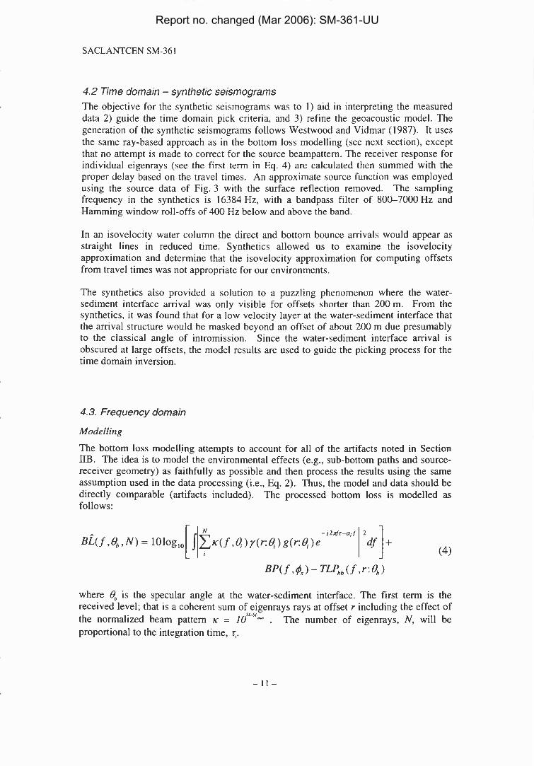
The bottom loss modelling attempts to account for all of the artifacts noted in Section IIB. The idea is to model the environmental effects (e.g., sub-bottom paths and source- receiver geometry) as faithfully as possible and then process the results using the same assumption used in the data processing (i.e., Eq. 2). Thus, the model and data should be directly comparable (artifacts included). The processed bottom loss is modelled as follows:

where 8, is the specular angle at the water-sediment interface. The first term is the received level; that is a coherent sum of eigenrays rays at offset r including the effect of

sr-s; the normalized beam pattern K = 10 . The number of eigenrays, N, will be proportional to the integration time, q .


SACLANTCEN SM-36 1

The 113 octave frequency average is performed incoherently. Ray quantities y, g, r, and a respectively are the combined pressure reflection/transmission coefficient, the geometrical spreading, travel time, and attenuation for each ray i as computed following (Westwood and Vidmar (1987)). The model is capable of predicting effects of shear waves. However, for the environment examined in this paper shear waves contributed negligibly and thus are not included in the analysis. The second and third terms mirror the assumptions in the data processing (Eq. 2) by introducing a normalized beam pattern correction BP at the nominal source angle 4 and a correction for the transmission loss TLP,, at the nominal bottom angle 8,.

Geoacoustic Extraction The frequency domain solution contains clues about the velocity structure of the sub- bottom that can refine the time domain picks. The frequency domain solution also contains important clues about the attenuation and density, the former being the most notoriously difficult parameter in a geoacoustic model to estimate.

As an initial geoacoustic model, density and attenuation are computed from empirical relationships following Bachman (1985) and Hamilton (1980)6 respectively using the velocity data as the known parameter. Forward modelling is then employed to refine these estimates by comparing the model output with the measured data over frequency and angular regions that are sensitive to each parameter. For example, the slope (in angle) of low angle bottom loss is often highly sensitive to the attenuation. This is due to the fact that at low frequencies, the dominant path for the energy is often refraction through the sediment. A linearly frequency dependent attenuation is assumed. There was no indication in the measured data that a non-linear frequency dependence was justified. Density effects are generally best observed near normal incidence where reflection rather than refraction dominates.

m e attenuation is derived from the porosity which is estimated using the Bachman (1985) relation between velocity and porosity.


SACLANTCEN SM-361

5 Discussion of Results

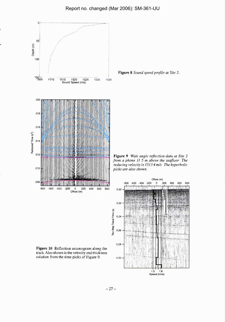
Our method has been employed at various locations in a shallow water region known as Capraia Basin in the northern Tyrrhenian Sea (see Fig. 2) as well as in on the Malta Plateau. Data from the north-south track at Capraia Site 2 on a hydrophone 12 m above the seafloor will be presented in this section. Bathymetry was essentially flat (150 m water depth) across the measurement area and the limiting angle at the seafloor based on the sound speed profile (see Fig. 8) is approximately 11".

5.1. Time domain - Bryan method In Fig. 9, the wide angle reflection data on the bottom hydrophone of the VLA is presented versus reduced time. This mapping has the desirable property that reflectors with the same stacking velocity (see Annex) have the same curvature regardless of their zero offset intercept time. It also allows a visual indication of where layers of lower sound speed relative to surrounding layers are located. The "picked" wide angle reflections used to obtain the thickness and interval velocity of the layers are also shown in this figure.

The velocity versus depth solution from the picks (converted to travel time) is superimposed on the reflection seismogram in Fig. 10. Note that in the reflection seismogram that the sub-seabed reflectors are laterally continuos and exhibit little range dependence. The quality of the reflection data was lower than that which is normally acquired. For example, there is a gap in the data until an offset of 183 m from the VLA and numerous spurious transient signals are present. However, we are confident that these are not actual point reflectors in the seabed as they are sometimes present as pre- seabed arrivals and no hyperbolic shaped diffraction arrivals are seen on adjacent seismograms. The interval velocity and thickness of the layers are provided in Table 1 along with the initial density and attenuation values.


SACLANTCEN SM-361

Table 1 Initial geoacoustic model

5.2. Frequency Domain In this section, results of the bottom loss (frequency domain) analysis are provided. In order to obtain the best possible depth resolution in the extracted geoacoustics, the bottom loss data were processed in cumulative time intervals. At this site, three cumulative windows were chosen, the first from 04 m sub-bottom, the second from approximately 0-9 m sub-bottom depth and the third from 0-25 m sub-bottom. In the following discussion we define the depth of these windows not in terms of the actual window length but rather in terms of the depth of the last layer horizon in the window. These windows were at 3 m, 5 m, and 23 m respectively sub-bottom. The analysis frequencies for each of the windows were changed slightly for each time window because the longer time windows yielded improved source level stability at lower frequencies due to transducer ringing (see Section IA), but degraded signal-to-noise ratio at the higher frequencies. Therefore the analysis frequencies (covering just over 2% octaves) are 1000-6300 Hz, 800-5000 Hz, and 6304000 Hz respectively. Bottom loss data on the incoming leg (south of the array) were essentially identical to the data on the outgoing leg (north of the array), indicating that the measurement area is laterally homogenous. Data are presented from the incoming leg.

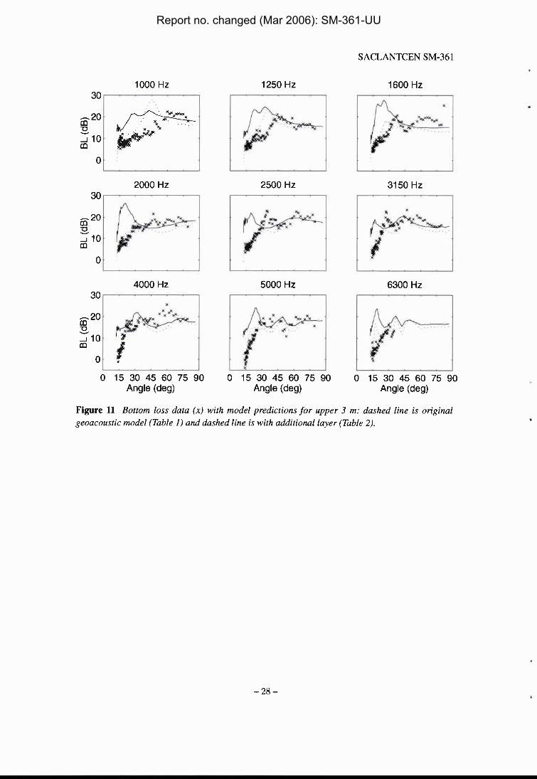
Figure 11 shows bottom loss data integrated to 3 m depth in sub-bottom. First note the characteristics of the measured data. The unusually high data density and lack of


SACLANTCEN SM-36 1

'random' scatter7 in the data provides features which can be exploited for extracting geoacoustic data. Now consider the model predictions shown in the solid line. Predictions from the baseline geoacoustic model (Table 1, first three layers only) are quite poor, especially at shallow grazing angles. A more careful examination of the time domain data indicated the presence of another layer between the first and second. These layer properties were estimated by a combination of the time and frequency domain data and are given in Table 2 (second layer). The resulting prediction (dotted line) in Fig. 11 is considerably better, especially at higher frequencies.

Table 2 Updated geoacoustic model for upper 3 m

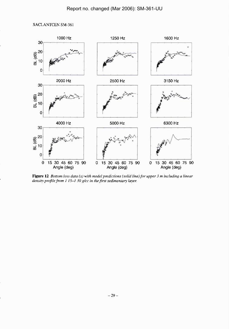
An even higher quality geoacoustic model was desired which lead to a sensitivity study. The sensitivity analysis showed that the bottom loss was very sensitive to density gradients in the first layer. Since the first layer has such a low velocity indicative of a very soft silty clay, a large gradient could be suggestive of the transition from a suspension to a sediment. Figure 12 shows the predictions using a linear density profile from 1.15-1.30 g/cc in the first layer; note that the fit is now quite good across angle and frequency. Some of the details in angular dependence are well-modelled, e.g., at 2500 and 3150 Hz. That the bottom loss was sensitive to the density gradient was a somewhat surprising result inasmuch as density gradients are often assumed to be unimportant in geoacoustic modelling [e.g., Rutherford and Hawker (1978)l. Corresponding to the density gradient there is almost certainly a velocity gradient. The predictions, however, are not sensitive to typical velocity gradients (less than 10 s-') in the upper layer. The predictions are sensitive to very large velocity gradients of order 50 s-'. For such large gradients the model predicts higher peaks in the bottom loss near 30" at 2500 and 3150 Hz in greater accord with the measurements. An analysis of sensitivity to attenuation for this 3 layer model indicated that Hamilton values were an upper bound. In other words, higher attenuation values gave poorer fits (especially at low angles and high frequencies), but lower values did not change the prediction at all. In general, for such short path lengths (3 metres to last reflecting horizon in the window) the model is not very sensitive to attenuation.

Thickness(m)

0.5 0.6 2.2 03

With the geoacoustic model set for the upper 3 m the next 2 layers from Table 1 are now added as shown in Table 3. Figure 13 shows bottom loss data integrated to 6 m depth in sub-bottom with the corresponding predictions. The predictions are quite good across angle and frequency indicating that the geoacoustic model is reasonable. Note for example the capability of the model to predict the low angle interference pattern caused

The usual angle averaging was not done.

Velocity (mls)

1486 155 1 1516 1527

Density (g/cc) 1.38 1.58 1.48 1.51

Attenuation (dB/m/kHz)

.07 0.1

.09 0.1


SACLANTCEN SM-36 1

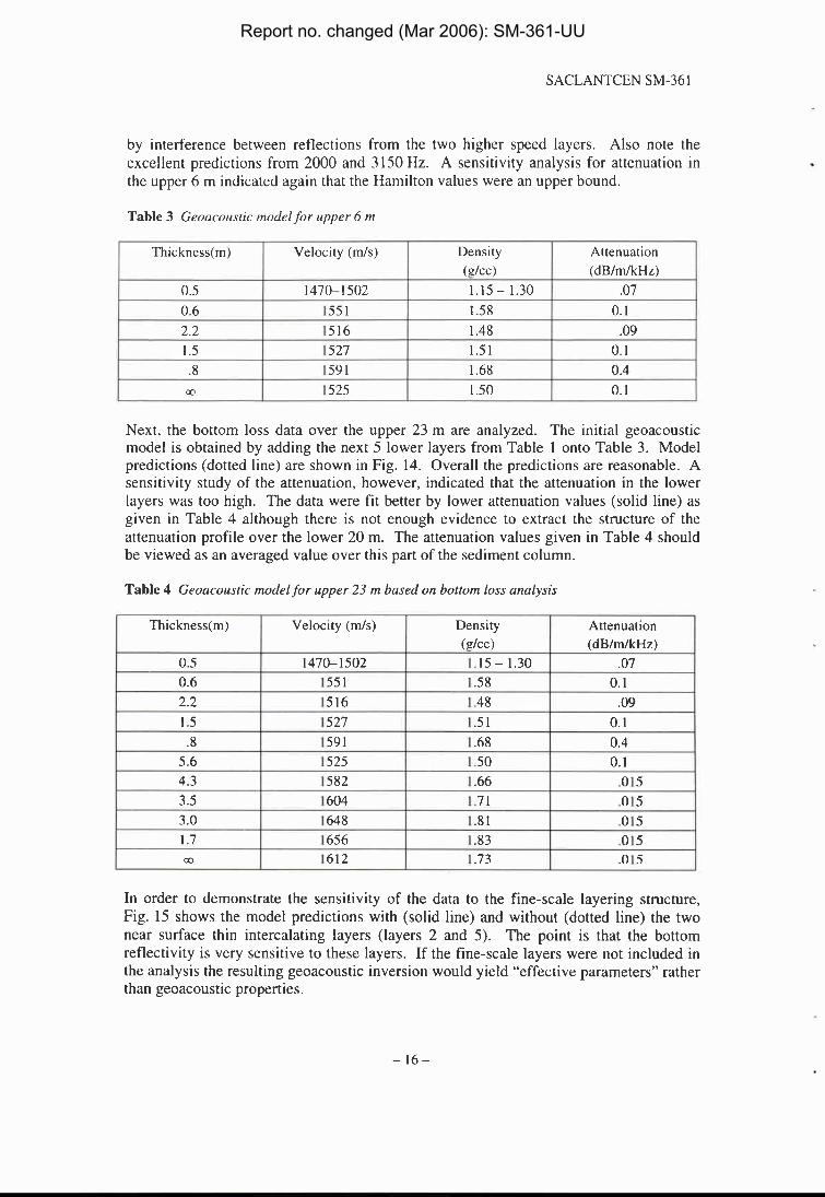
by interference between reflections from the two higher speed layers. Also note the excellent predictions from 2000 and 3150 Hz. A sensitivity analysis for attenuation in the upper 6 m indicated again that the Hamilton values were an upper bound.

Table 3 Geoacoustic model for upper 6 m

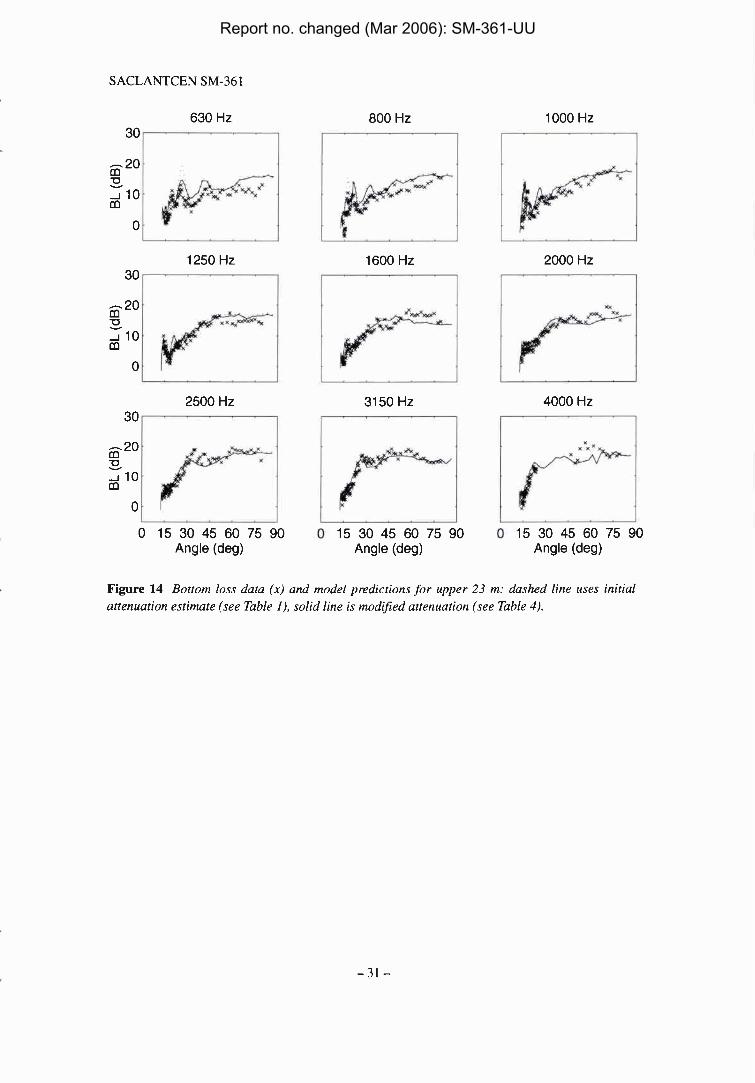
Next, the bottom loss data over the upper 23 m are analyzed. The initial geoacoustic model is obtained by adding the next 5 lower layers from Table 1 onto Table 3. Model predictions (dotted line) are shown in Fig. 14. Overall the predictions are reasonable. A sensitivity study of the attenuation, however, indicated that the attenuation in the lower layers was too high. The data were fit better by lower attenuation values (solid line) as given in Table 4 although there is not enough evidence to extract the structure of the attenuation profile over the lower 20 m. The attenuation values given in Table 4 should be viewed as an averaged value over this part of the sediment column.

Table 4 Geoacoustic model for upper 23 m based on bottom loss analysis

Thickness(rn)

0.5 0.6 2.2 1.5 .8 w

In order to demonstrate the sensitivity of the data to the fine-scale layering structure, Fig. 15 shows the model predictions with (solid line) and without (dotted line) the two near surface thin intercalating layers (layers 2 and 5). The point is that the bottom reflectivity is very sensitive to these layers. If the fine-scale layers were not included in the analysis the resulting geoacoustic inversion would yield "effective parameters" rather than geoacoustic properties.

Density (g/cc) 1.15 - 1.30 1.58 1.48 1.5 1 1.68 1.50

Velocity (rn/s)

1470-1502 155 1 1516 1527 159 1 1525

Attenuation (dB/rn/kHz)

.07 0.1

.09 0.1 0.4 0.1


SACLANTCEN SM-361

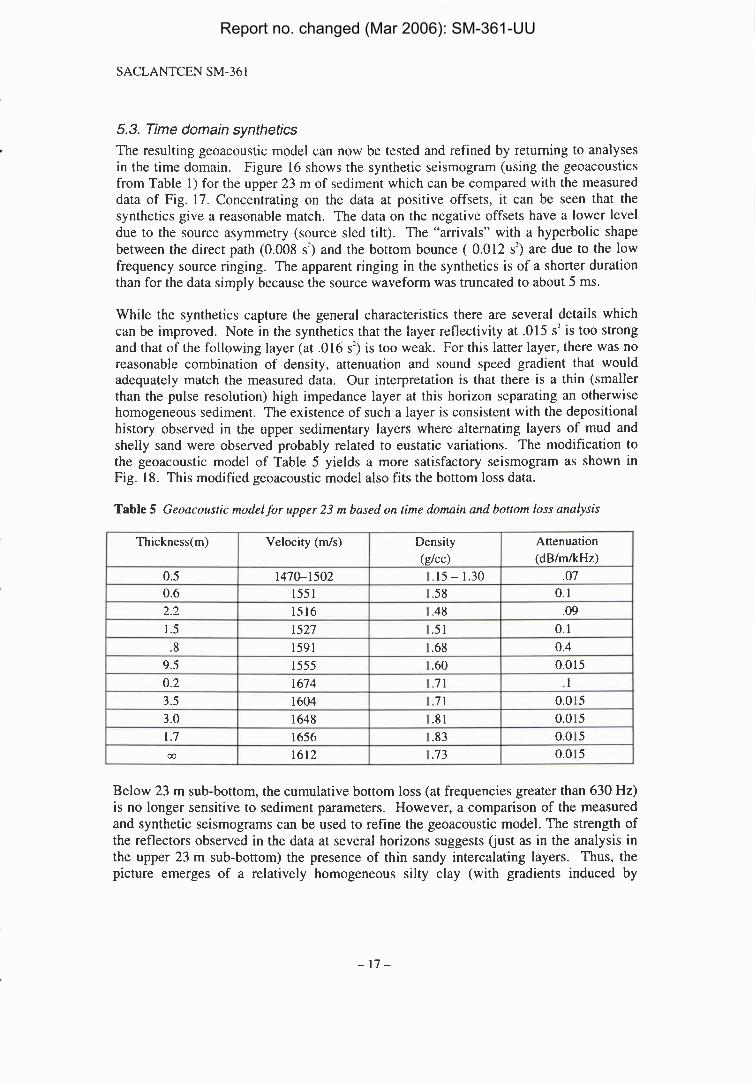
5.3. Time domain synthetics The resulting geoacoustic model can now be tested and refined by returning to analyses in the time domain. Figure 16 shows the synthetic seismogram (using the geoacoustics from Table 1) for the upper 23 m of sediment which can be compared with the measured data of Fig. 17. Concentrating on the data at positive offsets, it can be seen that the synthetics give a reasonable match. The data on the negative offsets have a lower level due to the source asymmetry (source sled tilt). The "arrivals" with a hyperbolic shape between the direct path (0.008 sZ) and the bottom bounce ( 0.012 s') are due to the low frequency source ringing. The apparent ringing in the synthetics is of a shorter duration than for the data simply because the source waveform was truncated to about 5 ms.

While the synthetics capture the general characteristics there are several details which can be improved. Note in the synthetics that the layer reflectivity at .015 s' is too strong and that of the following layer (at .016 s') is too weak. For this latter layer, there was no reasonable combination of density, attenuation and sound speed gradient that would adequately match the measured data. Our interpretation is that there is a thin (smaller than the pulse resolution) high impedance layer at this horizon separating an otherwise homogeneous sediment. The existence of such a layer is consistent with the depositional history observed in the upper sedimentary layers where alternating layers of mud and shelly sand were observed probably related to eustatic variations. The modification to the geoacoustic model of Table 5 yields a more satisfactory seismogram as shown in Fig. 18. This modified geoacoustic model also fits the bottom loss data.

Table 5 Geoacoustic model for upper 23 m based on time domain and bottom loss analysis

Below 23 m sub-bottom, the cumulative bottom loss (at frequencies greater than 630 Hz) is no longer sensitive to sediment parameters. However, a comparison of the measured and synthetic seismograms can be used to refine the geoacoustic model. The strength of the reflectors observed in the data at several horizons suggests (just as in the analysis in the upper 23 m sub-bottom) the presence of thin sandy intercalating layers. Thus, the picture emerges of a relatively homogeneous silty clay (with gradients induced by


SACLANTCEN SM-36 1

overburden pressure) and interspersed sandy layers that provide sufficient velocity contrast for a reflecting horizon to be visible in the seismic data.

Figures 19 and 20 show the synthetic and measured seismograms for the entire observable arrival structure (to 150 m sub-bottom). The second bottom reflected multiple is seen at about .08 s2. Note that the curvature of each layer is well-modelled, meaning that the velocity structure is correct. Thin intercalating layers have been inserted at the appropriate points. Their existence is strongly evident in the data, however, their geoacoustic characteristics (thickness, sound speed, density, and attenuation) are not particularly well constrained. The final geoacoustic model is shown in Table 6.

Table 6 Geoacoustic model for upper 150 m based on time domain and bottom loss analysis

Figure 21 shows the inverted interval velocity along with the empirical depth function suggested by Hamilton (1980) for deep water terrigenous sediments (silt clays, turbidities, mudstone shale). Note that in this shallow water environment the sound speed gradients are considerably higher than the Hamilton model allow, especially near the water-sediment interface. An alternative fit to the interval velocity is also shown which was based on a form for the sediment sound speed c(z) as proposed by Spofford et al. (1983)


SACLANTCEN SM-361

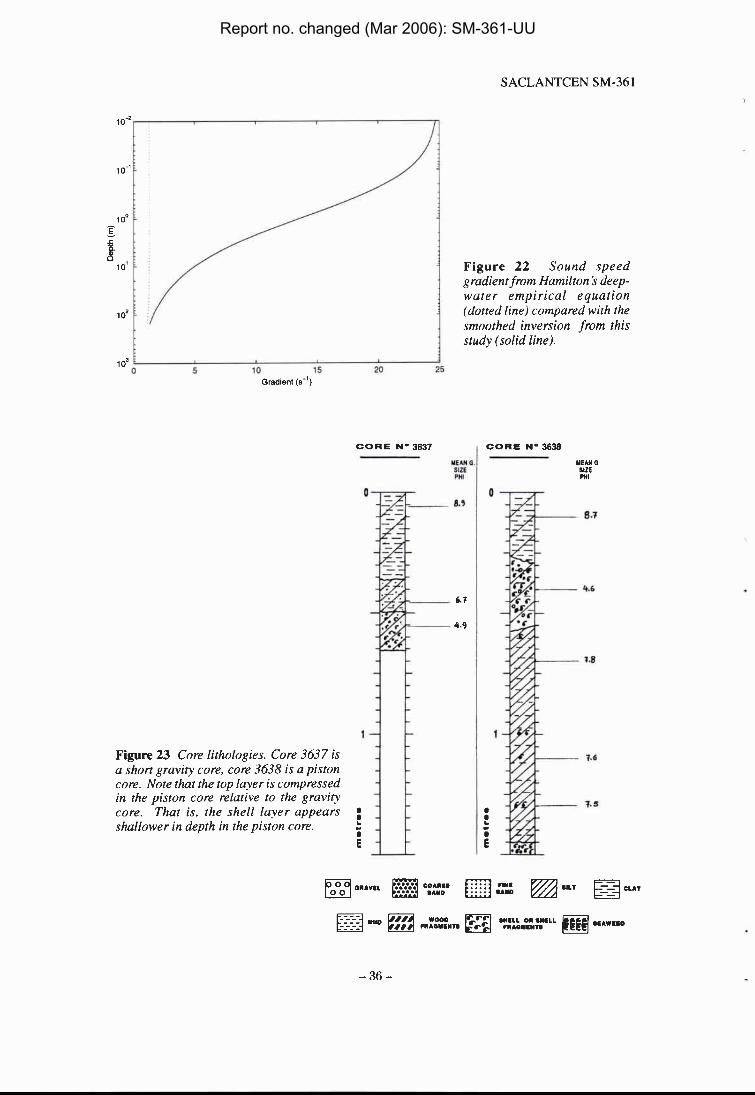
where z is depth in metres, c,, is the speed at the top of the sediment, g,, is the initial gradient and P is a parameter that controls the curvature. For the fit in Fig. 21 we have used c,, =I470 rn/s (from the inversion results), g,, = 25 s-' and P = -.986. Figure 22 shows a quantitative comparison of the depth dependence of the sound speed gradient from the fitted model and the Hamilton empirical equation.

5.4 Ground truthing It would be desirable compare the geoacoustic model of Table 6 with independent ground-truth. However, there does not exist any reliable ground truthing method for the complete model, to 150 m in sub-bottom depth. One potential means is by coring, however, coring has limitations because the sediment fabric is often disturbed by the coring operation as well as by post-core handling. Also core velocity measurements are prone to error because they are taken at much higher frequencies (200 kHz in our case) and suffer from scattering from small pebbles and shell fragments. Thus, core data can be considered to be valuable additional information, but not necessarily ground truth.

Two short cores (of order 1 m) were taken at this site, one gravity core (#3637) designed to minimize disturbance of the sediment and one piston core (#3638) intended for deeper penetration with greater likelihood of sediment disturbance. Sound speed measurements were taken at 200 kHz shortly after the cores were collected. Several months after collection, the cores were split, logged, md measured for mass properties (including density). Some of the cores showed evidence of settling from 2-4 cm over this time period. Therefore, the velocity measurements are the most reliable in terms of minimal core disturbance caused by handling.

The lithology of the cores is shown in Fig. 23 which shows a predominantly mud bottom with intercalating layers of shelly sand with some coral fragmentss. For the piston core, the upper layer is compressed about 30% relative to the gravity core. This most probably stems from core collection problems associated with the piston. This compression is also visible in the velocity and density measurements shown in Fig. 24. In the shelly layer, the shells were quite large having length scales on the order of 2 4 cm, the largest had an area of about 6 cm by 6 cm. Since these densely packed inclusions were on the order of a wavelength the velocity measurements in the shell layers are probably not reliable.

Figure 24 also contains the inversion results. There are a number of promising similarities between the inversion results and the core data. First, both show the 50 cm low speed layer at the water-sediment interface. Both also show large gradients in this layer, although the measured gradients are even larger than the inversion results. Second, note the manifestation of the higher speed shelly layer in both the inversion and the core data. Since the core velocity measurements are probably contaminated in this layer a quantitative comparison can not be made. Third, note that the inversion and the core sound speed measurements are very similar below the shelly layer. Fourth, note the density gradient in the core measurements which was crucial for the good model-to-data

The shells and shell fragments were bivalves (from the Tellinid and Pettinid families) and prosobranches (Tunitellid and Vermetid families). The coral fragments were Arborascente.


SACLANTCEN SM-36 1

agreement in Fig. 12. The major difference in the comparison is that the inversion density results appear to be lower than the core measurements. This may be due in part to core disturbance during storage and shipping. It may also be due to the fact that the inversion technique can extract information about density differences but not absolute densities.


SACLANTCEN SM-361

Summary

A method has been presented for obtaining high resolution geoacoustic properties from the seafloor. The high resolution in depth stems from using a short pulse, with a dense spatial sampling over a fairly short aperture (of order several hundred metres). Layers of order 50 cm were identified and geoacoustic data were recovered to depths greater than 100 m. The best quality data were extracted from the upper 23 m. Depth of penetration will be depend on the sub-bottom structure with a maximum penetration of one water depth.

The short measurement aperture means that the measurements are "local", i.e., they are applicable over a confined area. A later paper will explore the potential for extrapolating these "local" measurements to a regional model using seismic data to connect various sites.

The strength of the method lies in the wide range of data employed: including the time, frequency and spatial domains. Using as much independent data as possible provides the basis for inversion of geoacoustic properties rather than effective parameters. Whether the geoacoustic data obtained from the inversion in this paper are properties, is difficult to determine since there is no means for determining "ground truth" for any of these properties to depths of 150 m sub-bottom. Core velocity and density data in the upper 1.5 metres did compare favorably with the inverted data.

Finally, sound speed gradients appear to be much larger in this shallow water environment than the deep-water Hamilton empirical equations would suggest down to 100 m sub-bottom. Near surface (within the first meter) velocity and density gradients were extremely large, approximately 150 s" and 1.2 gfcclm respectively.

Acknowledgments

We wish to acknowledge the captain, officers, crew and the entire scientific crew aboard the Alliance who managed the ship manoeuvers and data collection effort with adeptness and aplomb. We express particular appreciation of Mr. Luigi Troiano and Mr. Piero Boni, whose engineering and data acquisition skills and initiative were crucial to the success of the experiment. Special thanks to Dr. Reg Hollett for help in the bottom loss data processing.


SACLANTCEN SM-36 1

References

Al-Chabali, M. Series approximation in velocity and traveltime computation. Geophysical Prospecting, 21, 1973:783-795. Bachman, R.T., Acoustic and physical property relationships in marine sediments. Journal of the Acoustical Society of America, 78, 1985:616-621. Bryan, G. M. The hydrophone-pinger experiment. Journal of the Acoustical Society of America, 68, 1980:1403-1408. Bryan, G. M. Sonobuoy measurements in thin layers. In: Lloyd Hampton (editor), Physics of Sound in Marine Sediments. New York, Plenum, 1974:119-130. Claerbout, J. F. How to derive interval velocities using a pencil and a straight edge. Stanford Exploration Project Report No. 14,1978. Dix, C. H. Seismic velocities from surface measurements. Geophysics, 20, 1955:68-86. Hamilton, E.L. Geoacoustic modelling of the seafloor. Journal of the Acoustical Society of America, 68, 1980: 13 13-1339. Gerstoft, P., Gingras, D. Parameter estimation using multifrequency range-dependent acoustic data in shallow water. Journal of the Acoustical Society of America, 99, 1996:2839-2850. Holland, C.W., Neumann, P. Sub-bottom scattering: a modelling approach. Journal of the Acoustical Society of America, 104, 1998: 1363-1 373. Le Pichon, X., Ewing, J., Houtz, R.E. Deep-sea sediment velocity determination made while reflection profiling. Journal of Geophysical Research, 73, 1968:2597-2614. Mitchell, S.K., Focke, K.C. New measurements of compressional wave attenuation in deep ocean sediments. Journal of the Acoustical Society of America, 67, 1980: 1582-1589. Osler, J.C., Holland, C.W., Fracassi, U. High resolution velocity inversion from shallow water wide angle seismic reflection measurements, SACLANTCEN SM-353. Rutherford, S.R. Hawker, K.E. Effects of density gradients on bottom reflection loss for a class of marine-sediments. Journal of the Acoustical Society of America, 63, 1978:750-757. Spofford, C.W. Greene R.R., Hersey, J.B. The estimation of geoacoustic ocean sediment parameters from measured bottom-loss data. SAIC Technical Report 83-879-WA, McLean, VA (1983). Taner, M. T., Koehler, F. Velocity spectra-digital computer derivation of velocity functions. Geophysics, 34, 1969959-881. Westwood, E.K. Vidmar, P.J. . Eigenray finding and time series simulation in layered bottom ocean. Journal of the Acoustical Society of America, 81, 1987:912-924.


SACLANTCEN SM-361

Figrnt 1 Experiment geometry.

Longitude (deg)

Figure 2 Capraia Basin area showing test sites (3, Elba Island is on the southern edge of the map Data analyzed in this paper collected at Site 2 which is on the 150 m contour Insert shows the general location on the northwest coast of Italy.


SACLANTCEN SM-36 1

0 8 10 15 Time (ms)

Figure 3 Uniboom source pulse at 19 cm depth received at a depth and offset of about 138 m and 15 m respectively.

Figure 4 Ray diagram of direct and bottom bounce naths with the asso>iated surface reflections.


SACLANTCEN SM-361

Source Angle (deg) Source Angle (deg) Source Angle (deg)

Figure 5 Comparison of measured data (dot) with extracted beam pattern (solid line) and a simple piston model (dashed line).


SACLANTCEN SM-361

315.0 500.0

Off set (m) Off set (m) Offset (m)

Figure 6. Dependence of source characteristics (direct path received level) on integration time for integration times of 24 ms (triangle), 12 ms (+) and 6 ms (dot). Data are plotted relative to an integration time of 48 ms.

- A - -

Figure 7 Ray diagram of the experiment geomtry showing the non-plane wave nature of the measurement technique That is, sub-bottom paths arrive at different angles than the specular.


0

50 / J-

a

, Figure 8 Sound speed profile at Site 2. 1

1520 1525 1530 1535 Sound Speed (mls)

a go0 400 -200 0 200 400 8QO 800 Offset (m)

Figure 10 Reflection seismogram along the track Also shown is the velocity and thickness solution from the time picks of Figure 9.

Figure 9 Wide angle reflection data at Sire 2 from a phone 11 5 m above the seafloor The reducing velocity is 1513 4 rn/s The hyperbolic picks are also shown.

Offset (m) "8w -400 -200 0 200 400 em 8a0

1.5 1.8 Speed (kmts)


0 15 30 45 60 75 90 0 15 30 45 60 75 90 Angle (deg) Angle (deg)

SACLANTCEN SM-361

1600 Hz

0 15 30 45 60 75 90 Angle (deg)

Figure 11 Bottom loss data (x) with model predictions for upper 3 m: dashed line is original geoacoustic model (Table I ) and dashed line is with additional layer (Table 2).


SACLANTCEN SM-361

I . . . . I

L J

0 15 30 45 60 75 90 Angle (deg)

0 15 30 45 60 75 90 Angle (deg)

0 15 30 45 60 75 90 Angle (deg)

Figure 12 Bottom loss data (x) with model predictions (solid line) for upper 3 m including a linear density profile from 1 15-1 30 g/cc in the first sedimentary layer:


0 15 30 45 60 75 90 Angle (deg)

0 15 30 45 60 75 90 Angle (deg)

SACLANTCEN SM-361

1250 Hz

0 15 30 45 60 75 90 Angle (deg)

Figure 13 Bottom loss data ( x ) and model predictions (solid line) for upper 6 m.


SACLANTCEN SM-36 1

- 0 15 30 45 60 75 90

Angle (deg) 0 15 30 45 60 75 90

Angle (deg) 0 15 30 45 60 75 90

Angle (deg)

Figure 14 Bottom loss data (x ) and model predictions for upper 23 m: dashed line uses initial attenuation estimate (see Table I ) , solid line is modified attenuation (see Table 4).


SACLANTCEN SM-361

1 - - . - . I

0 15 30 45 60 75 90 Angle (deg)

0 15 30 45 60 75 90 Angle (deg)

0 15 30 45 60 75 90 Angle (deg)

Figure 15 Bottom loss data ( x ) and model predictions for upper 23 m: solid line is with all layers (see Table 4), dotted line is with the intercalating layers (layers 2 and 5 ) removed.


-600 SM) -400 -200 0 200 400 600 800 Offset (m)

Figure 17 Wide angle seismogram for upper 25 m of sediment.

Figure 16 Synthetic seismogram for upper 25 m of sediment using inputs from Table 4.

-800 -600 -400 -200 0 200 400 600 800 Offset (rn)


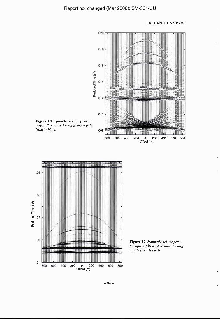
Figure 18 Synthetic seismog, upper 2.5 m of sediment using from Table 5.

ram for inputs

SACLANTCEN SM-36 1

-800 -800 -400 -200 0 200 400 600 800 Offset (rn)

Figure 19 Synthetic seismogram for upper 1.50 m of sediment using inputs from Table 6.

800 -800 400 -200 0 200 400 800 800 Offset (rn)


SACLANTCEN SM-361

Figure 20 Wide angle seismogram for upper 150 m of sediment.

-200 0 200 Offset (m)

- E - C 8 n

1W- -

lsbo

Figure 21 Interval velocity structure from the inversion (sol id stair step l ine) compared with Hamilton S empirical equation (dotted line) and a jit through the center of the layers (solid curved line) that appear to be the same sediment type.

2ow


SACLANTCEN SM-36 1

Gradient ( d l )

CORE No 3637

Figure 23 Core lithologies. Core 3637 is a short gravity core, core 3638 is a piston core. Note that the top layer is compressed in the piston core relative to the gravity core. That is, the shell layer appears shallower in depth in the piston core.

Figure 22 Sound speed gradient from Hamilton 5 deep- water empirical equation (dotted line) compared with the smoothed inversion from this study (solid line).

MEAN 0 SIZE CHI


SACLANTCEN SM-361

1.5 1500 1550 1600 1650

Sound Speed (mls) Density (glcc)

Figure 24 Comparison of inversion results (dashed line) with piston core (dotted line) atlrl gravity core (solid line) measurements. Above the water-sediment interface (0 m) are shorvrl the wnter columt~ values of density and sound speed.


SACLANTCEN SM-36 1

Annex A

Theory Following Bryan (1974, 1980) and Claerbout ( 1978), consider a homogeneous layer of velocity, v, , bounded by reflectors at depths, h , and h+h. As with the Dix (1955) and Le Pichon et al. (1968), it is assumed that velocity is a function of depth only. A given ray parameter, p , defines a path to each reflector (Fig. Al). In the ray parameter approach, these two paths are not associated with the same value of x (as would be the case in the Dix method), but rather with the same value of p , and above h , they are everywhere parallel. Thus, the contribution from the structure above h has cancelled out because of the choice of paths. The difference in travel time and offset for these two paths are

k ( p ) = ~ ~ + f pv/~- I - p-v- dh and

For a uniform velocity in the layer, vj , Eq. A1 can be integrated to give

AX = 2 pv,h, /dm and

which can be solved for the velocity and thickness of the layer,

v, = /" and PA^


SACLANTCEN SM-36 1

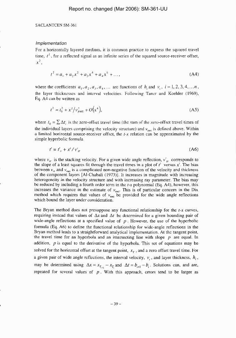
lmplemen ta tion For a horizontally layered medium, it is common practice to express the squared travel

2 time, t , for a reflected signal as an infinite series of the squared source-receiver offset, 7

x-.

where the coefficients a , , a,, a,, a,, . . . are functions of hl and v, , i = 1, 2, 3 ,4 , . . . n , the layer thicknesses and interval velocities. Following Taner and Koehler (1969), Eq. A4 can be written as

where to = 1 Atl is the zero-offset travel time (the sum of the zero-offset travel times of the individual layers comprising the velocity structure) and v,,, is defined above. Within a limited horizontal source-receiver offset, the t-x relation can be approximated by the simple hyperbolic formula

where v, is the stacking velocity. For a given wide angle reflection, vZn corresponds to the slope of a least squares fit through the travel times in a plot of t2 versus x2. The bias between v,, and v,, is a complicated non-negative function of the velocity and thickness of the component layers [Al-Chabali (1973)l. It increases in magnitude with increasing heterogeneity in the velocity structure and with increasing ray parameter. The bias may be reduced by including a fourth order term in the t-x polynomial (Eq. A4), however, this increases the variance in the estimate of v,,,. This is of particular concern in the Dix method which requires that values of v,, be provided for the wide angle reflections which bound the layer under consideration.

The Bryan method does not presuppose any functional relationship for the t-x curves, requiring instead that values of Ax and At be determined for a given bounding pair of wide-angle reflections at a specified value of p . However, the use of the hyperbolic formula (Eq. A6) to define the functional relationship for wide-angle reflections in the Bryan method leads to a straightforward analytical implementation. At the tangent point, the travel time for an hyperbola and an intersecting line with slope p are equal. In addition, p is equal to the derivative of the hyperbola. This set of equations may be solved for the horizontal offset at the tangent point, x, , and a zero offset travel time. For a given pair of wide angle reflections, the interval velocity, v, , and layer thickness, h, , may be determined using Ax = xT+, - xT and At = bj+, - b, . Solutions can, and are, repeated for several values of p . With this approach, errors tend to be larger as


SACLANTCEN SM-361

p approaches its minimal and maximal value. In the former case, because the values of Ax are very small and in the latter case, because it is increasingly rapidly.

As wide-angle reflections are represented by hyperbolae (Eq. A6), the maximum horizontal offset that is used must be selected with care. In order to work at larger horizontal source-receiver offsets, the use of a fourth order polynomial to represent the t- x curves was pursued. However, there are no straightforward analytical solutions to the system of equations described above and numerical solutions using Newton's method were prone to finding local minima. An alternate approach, therefore, was to also consider the maximum horizontal source-receiver offset which could be employed when testing the layer thickness and velocity resolution capabilities of the Bryan method with synthetic data.

Testing A number of test geoacoustic models were constructed and are described in detail in Osler et al. (in press). They all included a water depth of 150 m (characteristic of the depths in which SACLANTCEN shallow water experiments have been conducted) underlain by a seabed comprised of multiple isovelocity layers, including cases with low velocity zones. The thickness of the three seabed layers was varied in unison from 50 m to 1 m, yielding water depth to layer thickness ratios ranging from 3 to 150. For each geoacoustic model, theoretical travel times are calculated and then subjected to the analysis procedure outlined above.

Test results in Bryan (1974) using synthetic data indicate that solutions using the exact ray-parameter method deteriorate for thickness ratios of 100 or greater due to increasing relative error in Ax (Eq. A3) as Ax itself decreases with layer thickness. Further, his experience with real data suggest the method was useful up to thickness ratios of 25 and that another method, the thin layer approximation, should be used for thickness ratios greater than 50. When an appropriate horizontal source-receiver offset is selected, our test results suggest that the exact ray-parameter method is well behaved over a wider range of thickness ratios. The discrepancy between test results likely stems from different implementations of the method. Unfortunately, Bryan provides few details, but a potential explanation is that our analytical implementation serves to minimize errors in Ax.


SACLANTCEN SM-361

Time

I Distance

Depth Figure A1 Schematic diagram ofthe ray-parameter method (after Bryan, 1974). Note that the two ray paths are everywhere parallel above the first rejlector at depth h.


NATO UNCLASSIFIED

Document Data Sheet NATO UNCLASSIFIED . Project No.

042- 1

Total Pages

47 PP.

Security Classification

UNCLASSIFIED

Document Serial No.

SM-361

Date of Issue

December I998

A uthor(s)


Title

High resolution geoacoustic inversion in shallow water: a joint time and frequency domain technique.

Abstract " F'

High resolution geoacoustic data are required for accurate predictions of acoustic propagation and scattering in shallow water. Since direct measurement of geoacoustic data is difficult, time-consuming and expensive. inversion of acoustic data is a promising alternative. However, the main problem encountered in geoacoustic inversion is the problem of uniqueness, i.e., many diverse geoacoustic models can be made to fit the same data set. A key, and perhaps unique, aspect of this approach is the combination of data analysis in both the space-time and the space-frequency domains. This combination attempts to ameliorate the uniqueness problem by incorporating as much independent data as possible in the analysis. In order to meet the stringent requirements of high spatial resolution and uniqueness, an entire method has been developed including a new measurement technique, processinglanalysis technique, and inversion strategy. In this paper we describe each of these techniques and then show how they were applied to a shallow water data set in the Mediterranean Sea. The resulting sound speed R"' gradients in the upper 150 m sub-bottom appear much higher (one order of magnitude) than generally assumed. Inversion results in the upper several m~.~~kompare'-favorably with core analy$~*~ ...,>?&q

. ... .,.- a - ... 1:: ;-,q?..,+jfi ;$! = L : q ! p ,$ * ,; >

, ,+ l;ii.l ?A . J fi; , , rn ,: > ; + X z

.- i ; T - > . i" $' ";r. . -4%: '.:remu u'r ', ,- 'I,iiy.m.:J:

9 .... .,,;&"(:>+i: $

, .::$.ip;~ .-..-,I ;: 5%

*..>J>. $. rr2+ +.;y . ., . ; .- .-

1 :. . : - ,, - . . . . -.:7 ' . .. -!.: 4:

Keywords :.? -. , . .

Geoacoustic inversion, shallow water, sediment la;&ing, bottom reflection, sediment sound speed gradients

Issuing Organization

North Atlantic Treaty Organization SACLANT Undersea Research Centre Viale San Bartolomeo 400, 191 38 La Spezia, Italy

[From N. America: SACLANTCEN . (New York) APO AE 096131

Tel: +39 0187 527 361 Fax:+39 01 87 524 600

E-mail: library @saclantc.nato.int


gassie

Rectangle

gassie

Rectangle

Initial Distribution for Classified SM-361

Scientific Committee of National Representatives

SCNR Belgium SCNR Canada SCNR Denmark SCNR Germany SCNR Greece SCNR ltaly SCNR Netherlands SCNR Norway SCNR Portugal SCNR Spain SCNR Turkey SCNR UK SCNR USA SECGEN Rep. SCNR NAMILCOM Rep. SCNR

National Liaison Officers

NLO Canada NLO Denmark NLO Germany NLO ltaly NLO Netherlands NLO Spain NLO UK NLO USA

Sub-total SACLANTCEN library

Total


high resolution geoacoustic inversion in shallow water: a

Documents