high-resolution interpolar difference of atmospheric

Biogeosciences, 9, 3961–3977, 2012www.biogeosciences.net/9/3961/2012/doi:10.5194/bg-9-3961-2012© Author(s) 2012. CC Attribution 3.0 License.

Biogeosciences

High-resolution interpolar difference of atmospheric methanearound the Last Glacial Maximum

M. Baumgartner1,2, A. Schilt1,2, O. Eicher1,2, J. Schmitt1,2, J. Schwander1,2, R. Spahni1,2, H. Fischer1,2, andT. F. Stocker1,2

1Climate and Environmental Physics, Physics Institute, University of Bern, Sidlerstrasse 5, 3012 Bern, Switzerland2Oeschger Centre for Climate Change Research, University of Bern, 3012 Bern, Switzerland

Correspondence to:M. Baumgartner ([email protected])

Received: 16 April 2012 – Published in Biogeosciences Discuss.: 9 May 2012Revised: 28 August 2012 – Accepted: 14 September 2012 – Published: 16 October 2012

Abstract. Reconstructions of past atmospheric methane con-centrations are available from ice cores from both Greenlandand Antarctica. The difference observed between the two po-lar methane concentration levels represents a valuable con-straint on the geographical location of the methane sources.Here we present new high-resolution methane records fromthe North Greenland Ice Core Project (NGRIP) and the Eu-ropean Project for Ice Coring in Antarctica (EPICA) Dron-ning Maud Land (EDML) ice cores covering Termination 1,the Last Glacial Maximum, and parts of the last glacial backto 32 000 years before present. Due to the high resolution ofthe records, the synchronisation between the ice cores fromNGRIP and EDML is considerably improved, and the inter-polar concentration difference of methane is determined withunprecedented precision and temporal resolution. Relativeto the mean methane concentration, we find a rather stablepositive relative interpolar difference throughout the recordwith its minimum value of 3.7± 0.7 % between 21 900–21 200 years before present, which is higher than previouslyestimated in this interval close to the Last Glacial Maxi-mum. This implies that Northern Hemisphere boreal wet-land sources were never completely shut off during the peakglacial, as suggested from previous bipolar methane concen-tration records. Starting at 21 000 years before present, i.e.several millennia prior to the transition into the Holocene,the relative interpolar difference becomes even more pos-itive and stays at a fairly stable level of 6.5± 0.8 % dur-ing Termination 1. We thus find that the boreal and tropicalmethane sources increased by approximately the same factorduring Termination 1. We hypothesise that latitudinal shiftsin the Intertropical Convergence Zone (ITCZ) and the mon-soon system contribute, either by dislocation of the methane

source regions or, in case of the ITCZ, also by changing therelative atmospheric volumes of the Northern and SouthernHemispheres, to the subtle variations in the relative interpo-lar concentration difference on glacial/interglacial as well ason millennial time scales.

1 Introduction

Methane (CH4) is a trace gas with a global mean atmo-spheric concentration of about 1800 parts per billion by vol-ume (ppbv) today and contributed to the greenhouse effectwith a radiative forcing (relative to 1750 AD) of 0.5 Wm−2

in 2010 (Dlugokencky et al., 2011). The higher CH4 emis-sions in the Northern Hemisphere compared to the South-ern Hemisphere induce an interpolar concentration differ-ence (IPD) which today is (under the anthropogenic influ-ence) about 134± 7ppbv (7.6± 0.5%) averaged over theyears from 1985 to 2010 (Dlugokencky et al., 2011), wherethe uncertainty is the 1σ standard deviation over the se-lected time span. Knowledge of the past latitudinal sourcedistribution is valuable to understand the biogeochemicaland climatic changes occurring in glacials, interglacials, andduring rapid climate changes such as Dansgaard/Oeschger(DO) events. As the main control of the past IPD, we con-sider the latitudinal distribution of emissions from borealand tropical wetlands, which contribute 60–80 % to the to-tal natural source today (Denman et al., 2007). A recentmodelling study (Weber et al., 2010) estimates a 4–18 %smaller wetland area and a 35–42 % lower wetland CH4 fluxduring the Last Glacial Maximum (LGM) compared to thepreindustrial Holocene. Wetland CH4 productivity depends

Published by Copernicus Publications on behalf of the European Geosciences Union.

3962 M. Baumgartner et al.: Interpolar difference of atmospheric methane

on temperature, precipitation, and availability of organicmaterial. Recent satellite observations show that temperatureis the more critical factor in high northern latitudes and wa-ter table depth more dominant in the tropics (Bloom et al.,2010). Changes in the latitudinal distribution of tempera-ture and consequent changes in the latitudinal distributionof precipitation might have regulated changes in the wetlandsource distribution in the past.

The atmospheric concentration of CH4 is not only influ-enced by the sources, but also by the sinks. The major sinkis the oxidation in the troposphere by the hydroxyl radi-cal (OH), which has its maximum abundance in the tropics(Hein et al., 1997). CH4 has a mean atmospheric lifetime of8.7± 1.3 years today (Denman et al., 2007). The influenceon the atmospheric lifetime of CH4 of sink competitors suchas biogenic volatile organic compounds (BVOC) is still de-bated. WhileKaplan et al.(2006) invoke major changes inthe atmospheric lifetime due to large changes in the BVOCemissions over Termination 1,Levine et al.(2011) find theeffect of changes in BVOC emission to be compensated bythe effects of changes in air temperatures on humidities andgas-phase chemical kinetics.Levine et al.(2012) confirm thisstatement also for DO events, and suggest that the changes inCH4 are mainly source driven.

Ice cores from Greenland and Antarctica allow us to re-construct past atmospheric CH4 variations and hence to con-strain the latitudinal source distribution by the knowledgeof the IPD (Brook et al., 2000; Chappellaz et al., 1997;Dallenbach et al., 2000). In this study, we measure theCH4 concentration along the NGRIP (Greenland) and EDML(Antarctica) ice cores. In two-box and three-box model simu-lations, the measured concentrations are used as inputs to es-timate the source strengths in both the Northern and SouthernHemisphere. Finally, we discuss the processes which mighthave caused the observed changes in the past source distribu-tion.

2 New data

Figure1 presents the two new high-resolution atmosphericCH4 records measured along the NGRIP (blue, 469 newmeasurements) and EDML (red, 190 new measurements) icecores covering the time interval between 32 and 11 thousandyears before present (kyrBP) on the unified EDML gas agescale derived byLemieux-Dudon et al.(2010). This includesthe Younger Dryas (YD), the Bølling/Allerød (BA), the LGMand the response to the DO events 2, 3, and 4. Earlier pub-lished EDML data (EPICA Community Members, 2006) areincluded in our calculations, where 83 remeasurements showa mean difference of 0.3 ppbv and a standard deviation of13.9 ppbv. A few NGRIP data points published earlier (Schiltet al., 2010b) are included as well. The mean time resolu-tion is 43yr for NGRIP and 59yr for EDML on the unifiedEDML gas age scale. This is in the order of the width of the

gas age distributions of the enclosed air from NGRIP andEDML. Details about the measurement system are describedin Sect.2.3.

2.1 Synchronisation

Precise synchronisation between the ice cores from Green-land and Antarctica is a prerequisite to calculate the IPD ofCH4. The fast and strong variations in the greenhouse gasCH4 can be used to synchronise the gas ages from differ-ent ice cores (Blunier et al., 2007). Ironically, the existenceof the IPD, which we want to calculate based on a precisesynchronisation, renders the latter difficult, since for everytie point we assume a certain IPD value (e.g.Buiron et al.,2011). Based on the assumption that fast CH4 variationsoccur simultaneously in both hemispheres, our new high-resolution data improve the synchronisation of the NGRIPand EDML gas records. Particularly, a new tie point is de-fined at 20.9kyrBP, and the uncertainty of the tie pointsat the start and the end of DO event 2 is substantially re-duced. We use 29 CH4 tie points (TableA1, black trian-gles on top of Fig.1) to improve the synchronisation of theNGRIP CH4 record to the unified EDML gas age scale de-rived byLemieux-Dudon et al.(2010). The start of the slowCH4 increase at 18kyrBP is also used as a tie point, assumingconstant increase rates in both hemispheres. This assumptionis not necessarily true, since the IPD represents an additionaldegree of freedom and induces a substantial synchronisationuncertainty in this case. We thus apply a synchronisation un-certainty of this tie point of 500yr, which is much larger thanthat of rapid CH4 changes (≈ 50yr).

2.2 Gravitational fractionation

In the context of the calculation of the IPD, we have to dis-cuss the gravitational fractionation in the firn column whichdecreases the CH4 concentration at the close-off depth com-pared to the atmospheric value. The gravitational depletionin the considered time interval is relatively stable with meanvalues of 2.9± 0.6ppbv for NGRIP and 2.4± 0.4ppbv forEDML, where the close-off depth was calculated using thedensification model byHerron and Langway(1980) with anestimated temperature and accumulation rate history fromNGRIP (Johnsen et al., 2001; NGRIP Project Members,2004) and EDML (Ruth et al., 2007; EPICA CommunityMembers, 2006). The atmospheric IPD would thus be about0.5±0.7ppbv higher than the IPD measured in the ice cores.The effect on the relative interpolar difference (rIPD) is lessthan 0.1 %, which is small compared to the overall error.Thus, we do not correct the data for gravitational depletion,in line with previous ice core studies (e.g.Buiron et al., 2011;Stenni et al., 2011; Schilt et al., 2010a,b; EPICA Commu-nity Members, 2006; Huber et al., 2006; Spahni et al., 2005;Fluckiger et al., 2004).

Biogeosciences, 9, 3961–3977, 2012 www.biogeosciences.net/9/3961/2012/

M. Baumgartner et al.: Interpolar difference of atmospheric methane 3963

11 12 13 14 15 16 17 18 19 20 21 22 23 24 25 26 27 28 29 30 31 32Age (kyr BP)

350

400

450

500

550

600

650

700

750

800

CH

4 (pp

bv)

0

5

10

15

20

25

30

35

40

45

50

55

IPD (C

H4 ) (ppbv)

NGRIP newNGRIP previousNGRIP SplineEDML newEDML previousEDML Spline

DO2DO3

DO4

H1 H2 H3

5.6

± 0.

8%

6.6

± 1.

0%6.

8 ±

0.9%

7.6

± 1.

6%

6.1

± 0.

5%

3.7

± 0.

7%

7.1

± 0.

5%

5.0

± 0.

8%

5.4

± 1.

0%

2.9

± 2.

3%6.

2 ±

2.4%

6.7

± 0.

9%

(I) (II) (III) (IV) (V) (VI) (VII) (VIII) (IX)(X) (XI) (XII)

Fig. 1. Atmospheric CH4 concentration between 32 and 11kyr BP reconstructed from polar ice core measurements. Data from Greenland(NGRIP) are plotted as blue circles and data from Antarctica (EDML) as red diamonds. Earlier published data (NGRIP fromSchilt et al.(2010a) and EDML fromEPICA Community Members, 2006) are shown as open symbols. The splines through the data are calculatedaccording toEnting (1987) with a cutoff period of 350yr. Mean IPD values (Table1) are in green, where the horizontal bar and the greenshaded area indicate the time interval and the vertical error bar shows the standard error of the mean. Corresponding relative interpolardifference (rIPD) values are indicated as black numbers. Heinrich Events (H) 1 to 3 (Hemming, 2004) are indicated in brown. Tie points forsynchronisation (Sect.2.1) are indicated on the top as black triangles. All CH4 concentrations are synchronised to the unified EDML gas agescale derived byLemieux-Dudon et al.(2010).

2.3 Measurement system

We use a wet extraction technique according toChappellazet al. (1997) andFluckiger et al.(2004) to separate the en-closed air from the surrounding ice (sample size 40g, cor-responds to a depth interval of 3 and 5cm, for EDML andNGRIP, respectively). In brief, a sample is put in a smallglass container and after evacuation of the ambient air, theice is melted in a heat bath (50◦C) and refrozen from bot-tom to top on a cooling plate (−40◦C). The headspacevolume is expanded into an evacuated and temperature-controlled (−60◦C) sampling loop and analysed by gas chro-matography using a thermal conductivity detector (TCD)(N2 +O2 +Ar) and a flame ionisation detector (FID) (CH4).Two standard gases (CH4 concentration at 408ppbv and1050ppbv) are used to calibrate the detectors at hourly inter-vals. Each calibration is checked by a control measurementwith a third standard gas showing a mean concentration of529.4± 3.1ppbv over the entire measurement series. Inter-calibration measurements with NOAA standard gases showthat the Bern CH4 concentrations are about 1 % higher com-pared to measurements performed on the NOAA scale. Thereproducibility of measurements on natural ice samples wasfurther determined by the analysis of a series of 5 adjacent

samples in 18 depth intervals. 83 data points show a precisionof 6.2ppbv, where 7 points have been rejected because of toohigh values caused by badly sealed glass containers (morethan 3σ higher than the mean of the other reproducibilitymeasurements from the same depth-interval). In contrast toMitchell et al.(2011), who observe a loss of CH4 due to sol-ubility effects during the wet extraction process, blank mea-surements with air-free ice and standard gas show a concen-tration independent contamination (Chappellaz et al., 1997)on the order of 10 ppbv, depending on the particular glasscontainer. For each of the glass extraction containers, we de-termine a separate correction value, which is subtracted fromeach measurement on natural ice.

3 Interpolar concentration difference of CH4

The interpolar concentration difference of CH4 is a valuableconstraint on the geographical location of the CH4 sources.For the determination of the IPD of only a few ppbv, we mustexclude any systematic offsets between the CH4 records fromboth polar ice sheets. The sampling and measurement strat-egy of this study was designed for an optimum determina-tion of the IPD. For the first time, all the new data points are

www.biogeosciences.net/9/3961/2012/ Biogeosciences, 9, 3961–3977, 2012


analysed in the same laboratory, relative to the same standardgases and within the same year of measurement. On eachmeasurement day we analysed both samples from Greenlandand Antarctica. Samples of different ages were measured inrandomised order over the complete record to avoid system-atic drifts in the IPD. Due to the quasi-simultaneously anal-ysed samples, we are confident of the accuracy of the newIPD values. Note that there are still potential systematic er-ror sources like, for example, in situ production of CH4 bybacteria and/or chemical reactions in any of the ice cores.However, in situ production of CH4 in the dry snow zone ofpolar ice sheets has not been proven yet.

3.1 Definition and calculation of IPD and rIPD

We define the interpolar concentration difference of CH4 inan absolute (IPD) and a relative manner (rIPD) similar toBrook et al.(2000):

IPD = cn − cs (1)

and

rIPD =cn − cs

12 (cn + cs)

=IPD

12 (cn + cs)

, (2)

where cn (index n: Northern Hemisphere) andcs (indexs: Southern Hemisphere) represent the concentrations mea-sured along the NGRIP and EDML ice cores, respectively.

As described in Sect.2.1, the synchronisation uncertaintyis relatively small for most of the tie points. However, theCH4 synchronisation provides no information about the tim-ing between the tie points, where linear interpolation mustbe assumed. Therefore, we calculatecn, cs, and the IPD asmeans over specific time intervals instead of a continuousIPD record. By calculating a mean value, and not a time-weighted mean value as inChappellaz et al.(1997), we es-sentially assume constant CH4 levels within the intervals,since the mean value over an interval with, for example, twodifferent CH4 levels would only be the same as the time-weighted mean value if the data resolution is exactly constantover the whole time interval.

The uncertainty in the calculated IPD is dependent bothon the measurement and the synchronisation error. For theEDML measurement error, we assign the standard error ofthe mean to the mean valuecs of an interval. For the NGRIPrecord we basically do the same but use a Monte-Carlo ap-proach to simultaneously estimate the synchronisation er-ror. For a total of 105 simulations, we randomly changethe NGRIP start and end points of each interval. With theexception of the point at 24.4kyrBP, these start and endpoints coincide with the tie points. For each simulation, thenew NGRIP tie points are chosen randomly and uniformlydistributed within the synchronisation uncertainty aroundthe original tie points. Hereby, we assign a slightly differ-ent gas age to all NGRIP data points. For each simulation

i = 1. . .105 and time interval, the mean concentrationcn,iand the standard error SEi of the mean concentration arecalculated. The final mean NGRIP concentrationcn and itsmeasurement error are calculated as the mean of all simu-lated mean concentrationscn,i and the mean of all simulatedstandard errors SEi , respectively. The synchronisation erroris calculated as the standard deviation of all mean concentra-tionscn,i . Errors for the IPD and rIPD are calculated from thestandard errors ofcn, cs, and the synchronisation error.

The criterion of constant CH4 levels is not a reason-able assumption for the interval 17.8–14.8 kyrBP, wherethe CH4 concentrations in both hemispheres show approx-imately a linear increase. We thus calculate the IPD as themean difference between two linear fits through the data.In order to account for synchronisation uncertainties, theNGRIP tie points are varied and the error of the IPD is ob-tained as the standard deviation of all 105 simulated IPD val-ues.

Since the DO events 3 and 4 are too short to calculatea mean value over their duration, we estimate the IPD usingthe maximum atmospheric concentrations observed duringthe events (for more details see Sect.3.4).

3.2 IPD in specified time intervals

A complete list of specified time intervals (I)–(XII), whichcorrespond to the green shaded areas (plus DO events 3and 4) in Fig.1, and associated IPD and rIPD values aregiven in Table1. We observe a positive IPD and hencea predominance of northern hemispheric sources comparedto southern hemispheric sources throughout the record. Be-side the very low IPD value during DO event 3, which hasa large uncertainty, the minimum IPD of 13.8± 2.5ppbv(3.7± 0.7%) is observed just after DO event 2 (interval VI),which is within the time interval of maximum ice sheet extent(Clark et al., 2009). The maximum IPD of 43.5± 6.5ppbv(6.6± 1.0%) is observed during the BA (interval II).

We refrain from calculating the IPD in the time interval24.4–23.2 kyrBP because the EDML data are inconsistentwith the Talos Dome Ice Core Project (TALDICE) data (Bu-iron et al., 2011; Stenni et al., 2011). This inconsistency ismarked as the grey shaded interval in Fig.2. Before DOevent 2, TALDICE (yellow) and NGRIP (blue) show an in-crease in the CH4 concentration from 26kyrBP until the on-set of DO event 2. This pattern is visible in EDML (red)prior to 24kyrBP; however, just before DO event 2, the con-centration level drops suddenly to 365.2ppbv, correspond-ing to the grey shaded area in Fig.2. Remeasurements ofthe EDML samples in this 20 ppbv concentration dip con-firm the low concentration level and exclude a problem in themeasurement system. With the current time resolution of theTALDICE record, the EDML dip can not be entirely rejected.High-resolution measurements on other Antarctic ice coreswill be crucial to resolve this issue. We note that TALDICE



Table 1.List of time intervals where the IPD is calculated (see also Fig.1).

Interval Mean Age Duration NGRIP CH4 Error EDML CH4 Error IPD Error rIPD Error sn ss stot(yr BP) (yr) (points)∗ (ppbv) (ppbv) (points) (ppbv) (ppbv) (ppbv) (ppbv) (%) (%) (Tgyr−1) (Tgyr−1) (Tgyr−1)

(I) YD 12 078 742 21 506.9 1.8 22 479.5 3.2 27.4 3.9 5.6 0.8 96 48 143(II) BA1 13 339 792 34 686.0 4.2 13 642.5 4.0 43.5 6.5 6.6 1.0 135 58 193(III) BA2 14 044 617 29 655.0 3.1 11 612.1 4.3 42.9 5.5 6.8 0.9 130 54 184(IV) H1 16 254 3099 55 463.2 1.9 39 429.1 1.6 34.1 7.1 7.6 1.6 95 35 130(V) + St1 19 109 2611 63 395.9 1.2 29 372.5 1.3 23.4 2.0 6.1 0.5 77 35 112(VI) LGM 21 545 656 17 376.7 1.8 20 362.8 1.5 13.8 2.5 3.7 0.7 66 42 108(VII) DO2 22 605 984 35 419.0 1.8 28 390.2 1.1 28.9 2.1 7.1 0.5 84 33 118(VIII) St2 25 672 2568 34 387.2 2.1 49 368.2 1.4 19.0 3.1 5.0 0.8 72 38 110(IX) St2 27 108 306 14 408.3 2.9 11 386.7 1.9 21.6 4.0 5.4 1.0 77 39 116(X) o DO3 27 600 0 1 461.5 6.7 1 448.1 8.3 13.4 10.7 2.9 2.3 78 54 132(XI) o DO4 28 750 0 1 518.7 7.2 1 487.3 9.7 31.4 12.1 6.2 2.4 101 46 146(XII) St3 30 005 1531 32 421.9 2.4 21 394.3 2.2 27.5 3.8 6.7 0.9 84 35 119

∗ Due to the variation of the NGRIP tie points (Sect.3.2), this is the mean value of all simulations and might thus not be an integer number.o IPD estimate based on one point (maxima of DO event) and after application of the firn model.+ Used as reference interval in Fig.7d.

15 20 25 30Age (kyr BP)

350

400

450

500

550

CH

4 sou

th (p

pbv)

350

400

450

500

550

CH

4 north (ppbv)

NGRIPNGRIP SplineGRIP newGRIP previousEDMLEDML SplineTalos newTalos previous

DO2

DO3

DO4

Fig. 2. Remeasurements along the GRIP and TALDICE ice cores.For clarity reasons, data from Greenland (circles) and Antarctica(diamonds) are shown on different concentration axes. The NGRIP(blue,Schilt et al.(2010b) and new data) and EDML (red,EPICACommunity Members(2006) and new data) data are the same as inFig. 1. Additionally plotted are the previous GRIP record (Blunieret al., 1998; Dallenbach et al., 2000) (light blue) and the TALDICErecord (Buiron et al., 2011; Stenni et al., 2011) (yellow). New GRIPand TALDICE remeasurements are shown as big light blue and yel-low symbols, respectively. The grey shaded area marks the time in-terval, where the EDML record deviates from the TALDICE record.All CH4 concentrations are synchronised to the unified EDML gasage scale derived byLemieux-Dudon et al.(2010).

data suggest that the IPD would be similar as in the intervalbefore.

3.3 Comparison with previous results

Figure 3 shows a compilation of new and existing (Brooket al., 2000; Chappellaz et al., 1997; Dallenbach et al., 2000)

rIPD values. The new rIPD values between 21.9–17.8 kyrBPare in agreement withBrook et al.(2000) but are significantlylarger than the estimate fromDallenbach et al.(2000). Thisdifference results from a concentration offset between ournew NGRIP data and the previously measured Greenland IceCore Project (GRIP) data (Blunier et al., 1998; Dallenbachet al., 2000). Figure2 shows that the GRIP data (light blueline) tend to be up to 30ppbv lower than the NGRIP data(blue line) in certain time intervals. The GRIP data especiallyshow a larger bias towards lower concentrations. On the otherhand, Antarctic records are consistent with the new EDMLdata. We remeasured 18 data points (round light blue sym-bols) along the GRIP ice core and found a good agreementwith our new NGRIP concentration level. A contamination ofthe GRIP ice due to the long storage time and an accompany-ing gas loss (Bereiter et al., 2009) is unlikely, since we elim-inated about 5mm of the outer surface when preparing theice. The reliability among the new data emphasises the im-portance of measuring both hemispheric records in the samelaboratory, with the same extraction technique, and using thesame standard gases to correctly determine the IPD.

The rIPD values of the DO events 2 (7.1± 0.5%) and 4(6.2± 2.4%) are well in the range of previous results fromBrook et al.(2000) for DO event 8 (7.8± 2.0%) and withthe mean value over several DO events (7.5± 2.1%) fromDallenbach et al.(2000). The rIPD value for DO event 3(2.9± 2.3%) is lower but has a large uncertainty.

For the BA period, we find a rIPD value twice as largeas estimated byBrook et al.(2000) and Dallenbach et al.(2000). For the YD period, the new rIPD value is in agree-ment withDallenbach et al.(2000) and 1.5 times larger thanthe value fromBrook et al.(2000).

3.4 IPD during the DO events 3 and 4

In contrast to the other parts of the new CH4 record, theDO events 3 and 4 are too short to calculate the IPD asa mean over a specific time interval. Thus, we estimate the



0 5 10 15 20 25 30 35 40 45 50Age (kyr BP)

-4

-3

-2

-1

0

1

2

3

4

5

6

7

8

9

10

11

12

rIPD

CH

4 (%

)

300

350

400

450

500

550

600

650

700

750

800

CH

4 (ppbv)

rIPD this studyDällenbach et al., 2000Brook et al., 2000Chappellaz et al., 1997EDML CH4

mean interstadial

mean stadial

BA

YDDO2

DO3

DO4 DO5DO6

DO7

DO8

Fig. 3. Compilation of rIPD values for atmospheric CH4 reconstructed from polar ice cores. Values from previous studies are given in black(Chappellaz et al., 1997): based on GRIP, D47 and Byrd; blue (Brook et al., 2000): based on GISP2 and Taylor Dome; and grey (Dallenbachet al., 2000): based on GRIP, Byrd and Vostok. New values, corresponding to the time intervals of Fig.1 and Table1, are shown in pink. TheCH4 concentration from EDML is plotted in red. All data are synchronised to the unified EDML gas age scale derived byLemieux-Dudonet al.(2010).

interstadial IPD using an estimate of the maximum atmo-spheric concentrations observed during the events. However,because such fast and short atmospheric variations are atten-uated due to molecular diffusion and gradual bubble close-offin the firn of an ice sheet, we first apply a forward smooth-ing firn model (Schwander et al., 1993; Spahni et al., 2003)to take into account the different enclosure characteristics ofthe EDML and the NGRIP sites. Temperature and accumula-tion rate, which both strongly influence the firn structure, areassumed to be similar at both sites during stadial conditions(NGRIP:−50.5±6.6◦C, 0.054±0.020 mH2Oyr−1; EDML:−51.9± 1.4◦C, 0.030± 0.004 mH2Oyr−1). During the DOevents 3 and 4, both temperature (−43.6± 4.8◦C) and accu-mulation rate (0.086± 0.023 mH2Oyr−1) jump up to highervalues in the NGRIP ice core. The estimates are taken fromthe ss09sea age scale (Johnsen et al., 2001) based on theδ18O reconstructions (NGRIP Project Members, 2004) com-bined with the temperature-δ18O relationship derived fromδ15N measurements (Huber et al., 2006). The higher temper-ature and accumulation rate during the interstadial periodslead to weaker attenuation at NGRIP compared to the EDMLsite, where we assume a temperature of−50.2± 1.7◦C andan accumulation rate of 0.036± 0.006mH2Oyr−1 (EPICACommunity Members, 2006; Ruth et al., 2007). Without ap-plication of the firn model, the IPD would be overestimatedfor these two short interstadial periods. Consequently, the in-

terstadial rIPD recorded in the ice cores without enclosurecorrection represents an upper limit, which is 6.3 % for DOevent 3 and 9.3 % for DO event 4.

The application of the firn model helps to derive the inter-stadial IPD for DO event 3 and 4 more precisely. The modelneeds several input parameters. For the close-off density, thesurface density and the tortuosity at NGRIP and EDML, weuse the recent values specified bySpahni et al.(2003) forGRIP and EPICA Dome C, respectively. Since we use a for-ward smoothing model, we first need to estimate the atmo-spheric signal, which serves as input for the firn model. Theatmospheric signal is then attenuated due to molecular dif-fusion and gradual bubble close-off in the firn (Schwanderet al., 1993). The closed-off concentration, which we mea-sure, is different compared to the original atmospheric con-centration. Note that the estimation of the atmospheric signalhas no unique solution, since mathematically it is a decon-volution. We followSpahni et al.(2003) and simply linearlyscale the CH4 amplitude of the NGRIP signal to constructthe estimate of both the northern and southern atmosphericsignal.

The constructed northern atmospheric signal is the inputfor the firn model at the NGRIP site, where we apply threedifferent attenuation scenarios (mean [min,max]; Fig.4). Thesmallest root mean square difference between the output ofthe firn model and the measured NGRIP data is achieved



Age (kyr BP)28 28.5 2927 27.5 28

Age (kyr BP)28 28.5 2927 27.5 28

Age (kyr BP)28 28.5 2927 27.5 28

350

400

450

500

550

CH

4 (pp

bv)

DO3DO4

DO3 DO3DO4 DO4

NGRIP dataEDML datafirn modelfirn modelatm. northatm. south

A B C

maxIPD

min IPD best guess IPD

Fig. 4. Firn model applied on DO events 3 and 4. Shown are the NGRIP data (blue circles) and EDML data (red diamonds) correspondingto Fig. 1. Atmospheric signals constructed by linear scaling and shifting the NGRIP data are shown as dotted lines. The corresponding firnmodel output is shown in blue for NGRIP and in red for EDML.(A) Minimum IPD: minimum attenuation at NGRIP, maximum attenuationat EDML. (B) Mean IPD: mean attenuation at NGRIP, mean attenuation at EDML.(C) Maximum IPD: maximum attenuation at NGRIP,minimum attenuation at EDML.

when the linear scaling factor is 1.13 [1.06,1.19] for DOevent 3 and 1.08 [1.05,1.13] for DO event 4. The southernatmospheric signal, which is obtained by linear scaling ofthe CH4 amplitude of the NGRIP signal as well, is the in-put for the firn model at the EDML site, where we applyagain three different attenuation scenarios. The smallest rootmean square difference between the output of the firn modeland the measured EDML data is obtained by varying thelinear scaling factor (1.48 [1.35,1.62] for DO event 3 and1.11 [1.02,1.21] for DO event 4) and the offset between theNGRIP and EDML data, which has been assumed to be con-stant over the entire DO event.

The resulting IPD (13.4± 10.7ppbv for DO event 3 and31.4± 12.1ppbv for DO event 4) is calculated as the dif-ference between the maximum concentrations of the splines(cutoff period 100yr) through the atmospheric input signals,where the maximum attenuation at NGRIP is combined withthe minimum attenuation at EDML and vice versa. The re-sulting rIPD is(2.9±2.3%) for DO event 3 and(6.2±2.4%)

for DO event 4.

4 Source distribution of CH4

The new NGRIP and EDML records provide the concentra-tions of CH4 in the northern (cn) and southern (cs) hemi-spheres. This enables us to formulate a two-box model toestimate the CH4 source strength in the Northern (sn) andSouthern (ss) Hemispheres. In this two-box model, the north-ern box (0◦ N–90◦ N, index: n) and the southern box (0◦ S–90◦ S, index: s) account for 50 % of the total atmosphericvolume each. The mass balance (Tans, 1997) is given by:

dM

dt= S − � · M, (3)

M = m∗·

(cncs

), S =

(snss

), m∗

=m0

c0·Vhem

Vatm(4)

and

� =

(1τ

+1

τex−

1τex

−1

τex

1τ

+1

τex

), (5)

where M is a vector of the atmospheric CH4 burden(Tgbox−1). The factor m∗ converts the concentrations(ppbv) into mass (Tg) where we use the relation between amean atmospheric concentrationc0 = 1650ppbv and a cor-responding global atmospheric inventory ofm0 = 4800Tgfrom Steele et al.(1992). The volume of one hemisphereVhem is assumed to be 50 % of the total atmospheric vol-umeVatm, which induces a factor of12. S is a vector whichsummarises the CH4 sources(Tgyear−1), � is the exchangematrix with τ the atmospheric lifetime of CH4, andτex theinterhemispheric mixing time.

We initialise the model with a present-day source strength(490 Tgyr−1) and a source distribution fromFung et al.(1991) (scenario 7) combined with the mean values in theatmospheric concentrations of the years 1985–1987 fromAlert (Canada, 82.45◦ N) and South Pole (89.98◦ S) (Dlugo-kencky et al., 2011), and immediately findτ = 10.0yr andτex = 1.8yr. We keep these values fixed during all modelruns. The dependence ofsn andss on the parametersτ andτexis described in Sect.4.1. An alternative initialisation with asource strength estimate (548 Tgyr−1) and a source distribu-tion estimate for the year 2004 from a more recent CH4 bud-get modelling study (Spahni et al., 2011) yields τ = 9.5yrandτex = 1.7yr, which compare well with the above initiali-sation. Note that other studies using a two-box model (Sow-ers, 2010) lower the concentration measured in Greenlandcn



by a fixed portion of the IPD to obtain the mean concentra-tion of the northern box. This takes into account the latitu-dinally decreasing concentration from north to south withinthe northern box observed today. Due to the lack of the an-thropogenic sources, this latitudinal concentration gradientmight have been smaller in the past, however it might stillhave been present since it is mainly an effect of the sink,which is significantly lower at high latitudes. We did notlower the ice core derivedcn in our model study, but tookthis effect into account in our model initialisation by allow-ing for a relatively largeτex of 1.8yr. This essentially impliesthat this exchange time is representing the time needed forCH4 to sustain the measured interpolar, and not a mean inter-hemispheric concentration difference. If we had loweredcnby 26 % of the IPD (Sowers, 2010), the initialisation wouldyield τex = 1.3yr, which is well in range with the value fromGeller et al.(1997) (1.3±0.1yr) derived from sulfur hexaflu-oride (SF6).

The model is run for steady state conditions, which sim-plifies Eq. (3) and provides the sources:

sn (cn, IPD,τ,τex) = m∗·

(1

τ· cn +

1

τex· IPD

)(6)

and

ss(cs, IPD,τ,τex) = m∗·

(1

τ· cs−

1

τex· IPD

). (7)

The calculated source strengths corresponding to the meanconcentrations of the specified time intervals (Fig.1) areshown in Fig.5a and summarised in Table1. The errors forsn andss in this top-down simulation are calculated from theerrors ofcn andcs.

Vice versa in a bottom-up simulation, from a given sourcedistribution the two-box model provides the concentrationscn, cs and the IPD and rIPD:

IPD(sn, ss,τ,τex) =1

m∗· (sn − ss) ·

τ

1+ 2 ττex

(8)

and

rIPD(sn, ss,τ,τex) = 2 ·sn − ss

sn + ss·

1

1+ 2 ττex

. (9)

Hence, in this two-box model both the IPD and the rIPD areproportional to the differencesn − ss, but only the rIPD isindependent of global source scaling. This means that ifsnandss are scaled by the same factor, the rIPD stays constant.

For short exchange times,τex, the IPD is not especiallysensitive to the atmospheric lifetimeτ . However, for a givenvalue ofτex, rIPD decreases with increasingτ as the extentto which CH4 is mixed between hemispheres increases (andhence its concentration is homogenised globally).

4.1 Sensitivity of CH4 sources toτ and τex

Figure6 shows the sensitivity of the sourcessn andss, cal-culated in Eq. (6) and Eq. (7), to the parametersτ andτexfor three different time intervals (BA, YD, LGM). Relativelysmall changes in the two parameters have substantial impacton the estimated sources. For both parameters, the sensitivityis stronger for higher IPD. While changes in the atmosphericlifetime τ of CH4 primarily affect the total source strength,changes in the interhemispheric mixing timeτex affect thesource distribution.

Similar sensitivity experiments byBrook et al. (2000)with the three-box model show that for a fixed rIPD theboreal source increases and the tropical source decreaseswith decreasingτex (faster interhemispheric mixing). In thetwo-box model used in this study, assuming a fixed rIPD,sn would increase andss would decrease with decreasingτex (faster interhemispheric mixing). Conversely, assuminga fixed source distribution, a decrease inτex (faster inter-hemispheric mixing) would result in a decrease in the rIPD.Glacial/interglacial changes inτex could thus have affectedthe rIPD. If the interhemispheric mixing was faster in glacialtimes, this would imply that the northern source was strongerand the southern source weaker than estimated in this study.Further work is required to constrain the changes inτex onglacial/interglacial time scales.

4.2 Two-box model versus three-box model

Previous IPD studies used a three-box model to estimatethe CH4 source distribution (Chappellaz et al., 1997; Brooket al., 2000; Dallenbach et al., 2000). The three-box modelhas the advantage that it accounts for the higher sink strengthin the tropics compared to the high latitudes. Further, it pro-vides an estimate for the tropical source strength (30◦ N–30◦ S), but it is not able to distinguish between northern andsouthern tropical sources. Moreover, the source term for thesouthern box (30◦ S–90◦ S) has to be prescribed, becauseonly two measurements (Greenland and Antarctica) exist toconstrain the model.

The two-box model, on the other hand, has the advantagethat it is more illustrative and can be easily treated analyti-cally. Further, as already stated bySowers(2010), there is noneed to fix one source term. This is necessary in the three-boxmodel due to the missing information on the tropical concen-tration. Figure5b shows an alternative run with the three-boxmodel using exactly the model configuration fromChappel-laz et al.(1997). The southern source (30◦ S–90◦ S) is fixed at15 Tgyr−1 for the Holocene intervals including the YD andBA periods. For the glacial intervals it is fixed at 12 Tgyr−1.Overall, there is little difference in the output of the two mod-els. The trend insn of the two-box model is closely relatedto the trend in the boreal box of the three-box model (bluelines), while the trend inss follows the trend in the tropicalbox (red and green line). Adding the tropical source equally



0 10 20 30Age (kyr BP)

0

40

80

120

160

200

240

sour

ce s

tren

gth

(Tg

CH

4/yr)

400

500

600

700

CH

4 (ppbv)

3 box total3 box north3 box tropics3 box southEDML CH4

0 10 20 30Age (kyr BP)

0

40

80

120

160

200

240

sour

ce s

tren

gth

(Tg

CH

4/yr)

2 box total2 box north2 box southEDML CH4

3 box south + (3 box tropics)/23 box north + (3 box tropics)/2

BA

DO2DO3

DO4

DO2DO3

DO4

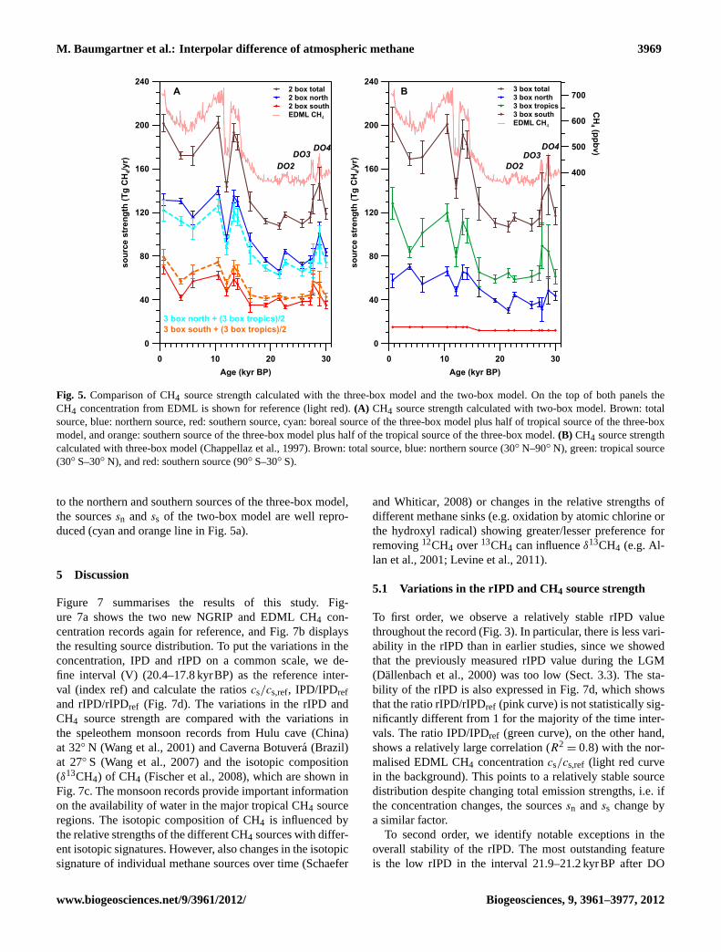
Fig. 5. Comparison of CH4 source strength calculated with the three-box model and the two-box model. On the top of both panels theCH4 concentration from EDML is shown for reference (light red).(A) CH4 source strength calculated with two-box model. Brown: totalsource, blue: northern source, red: southern source, cyan: boreal source of the three-box model plus half of tropical source of the three-boxmodel, and orange: southern source of the three-box model plus half of the tropical source of the three-box model.(B) CH4 source strengthcalculated with three-box model (Chappellaz et al., 1997). Brown: total source, blue: northern source (30◦ N–90◦ N), green: tropical source(30◦ S–30◦ N), and red: southern source (90◦ S–30◦ S).

to the northern and southern sources of the three-box model,the sourcessn andss of the two-box model are well repro-duced (cyan and orange line in Fig.5a).

5 Discussion

Figure 7 summarises the results of this study. Fig-ure 7a shows the two new NGRIP and EDML CH4 con-centration records again for reference, and Fig.7b displaysthe resulting source distribution. To put the variations in theconcentration, IPD and rIPD on a common scale, we de-fine interval (V) (20.4–17.8 kyrBP) as the reference inter-val (index ref) and calculate the ratioscs/cs,ref, IPD/IPDrefand rIPD/rIPDref (Fig. 7d). The variations in the rIPD andCH4 source strength are compared with the variations inthe speleothem monsoon records from Hulu cave (China)at 32◦ N (Wang et al., 2001) and Caverna Botuvera (Brazil)at 27◦ S (Wang et al., 2007) and the isotopic composition(δ13CH4) of CH4 (Fischer et al., 2008), which are shown inFig. 7c. The monsoon records provide important informationon the availability of water in the major tropical CH4 sourceregions. The isotopic composition of CH4 is influenced bythe relative strengths of the different CH4 sources with differ-ent isotopic signatures. However, also changes in the isotopicsignature of individual methane sources over time (Schaefer

and Whiticar, 2008) or changes in the relative strengths ofdifferent methane sinks (e.g. oxidation by atomic chlorine orthe hydroxyl radical) showing greater/lesser preference forremoving12CH4 over13CH4 can influenceδ13CH4 (e.g.Al-lan et al., 2001; Levine et al., 2011).

5.1 Variations in the rIPD and CH4 source strength

To first order, we observe a relatively stable rIPD valuethroughout the record (Fig.3). In particular, there is less vari-ability in the rIPD than in earlier studies, since we showedthat the previously measured rIPD value during the LGM(Dallenbach et al., 2000) was too low (Sect.3.3). The sta-bility of the rIPD is also expressed in Fig.7d, which showsthat the ratio rIPD/rIPDref (pink curve) is not statistically sig-nificantly different from 1 for the majority of the time inter-vals. The ratio IPD/IPDref (green curve), on the other hand,shows a relatively large correlation (R2

= 0.8) with the nor-malised EDML CH4 concentrationcs/cs,ref (light red curvein the background). This points to a relatively stable sourcedistribution despite changing total emission strengths, i.e. ifthe concentration changes, the sourcessn andss change bya similar factor.

To second order, we identify notable exceptions in theoverall stability of the rIPD. The most outstanding featureis the low rIPD in the interval 21.9–21.2 kyrBP after DO



5 10 15 20τ (years)

0

50

100

150

s n (T

g/yr

)

0

50

100

150

ss (Tg/yr)

YDBALGM

1 2 3 4τex (years)

0

50

100

150

s n (T

g/yr

)

0

50

100

150

ss (Tg/yr)

τex = 1.8 yr

τ = 10.0 yr

Fig. 6. Sensitivity of CH4 sources toτ and τex. Source distribu-tion (solid lines:sn, dashed lines:ss) calculated for three differentclimate states (blue: YD, red: BA, light blue: LGM; concentrationsfrom Table1) depending onτ (upper panel) andτex (lower panel).While one parameter is varied, the other is set toτ = 10.0yr orτex = 1.8yr (grey lines), accordingly. The model is run at these val-ues, which have their origin in the initialisation with a present-daysource distribution fromFung et al.(1991).

event 2. Both the decrease in the rIPD from DO event 2 tothis interval and the subsequent increase in the rIPD fromthis interval to the glacial reference interval 20.4–17.8 kyrBPare statistically significant. The same is true for the increasein the rIPD from the interval 27.0–24.4 kyrBP to the DOevent 2.

In the following we discuss in detail the time span aroundthe LGM, the Termination 1 (T1), and the DO events.

5.1.1 rIPD around the LGM

In the interval 21.9–21.2 kyrBP, we observe a pronouncedminimum in the rIPD. Together with this pronounced min-imum, but not significantly different from the reference in-terval, the interval 27.0–24.4 kyrBP shows one of the low-est rIPD values observed in the record. Especially in NorthAmerica, the boreal source is likely to be suppressed bythe wide extent of the ice sheets and permafrost regionsand hence is likely to contribute to the reduction of therIPD (Dallenbach et al., 2000; Fischer et al., 2008). Fur-ther, a bottom-up modelling study supports a southward shift

of the boreal and tropical sources in the LGM, which wascaused by a southward shift of the westerlies because of thelarge ice sheet extent and by a southward displacement of theITCZ, respectively (Weber et al., 2010).

A southward displacement of the ITCZ could influence therIPD in two ways. First, it would shift the optimal conditionsfor CH4 emissions to more southerly latitudes. The effecton the rIPD might be amplified by the coincident latitudi-nal dislocation of the monsoon systems. Second, a southwardshift in the ITCZ would increase the volume of the north-ern box at the expense of the southern box. A 1◦ southwardshift would change the volumes in the northern and southernbox by about 2 % in opposite directions. For 5◦ the volumechange of a box is 9 % and for 10◦ it is 17 %. If we assumethat the mixing time of a box is proportional to its volume,the two-box model simulates the volume changes caused bythe ITCZ shifts by using different mixing timesτex,n andτex,s for the northern and southern box. Assume now thatthe ITCZ was exactly at the equator during the glacial refer-ence interval (20.4–17.8 kyrBP). If we take the northern andsouthern emission strengths of the glacial reference intervalfrom Table1 (sn = 76.5Tgyr−1, ss = 35.3Tgyr−1) and varythe volumes of the northern and southern box, respectively,we find an alternative way to explain the rIPD variations ofthe glacial neighbour intervals. We need a 8.5◦ southwardshift of the ITCZ to explain the rIPD in the interval 21.9–21.2 kyrBP. Analogous, a southward shift of 4◦ is needed forthe interval 27.0–24.4 kyrBP and a northward shift of 3.5◦

for DO event 2.During the Holocene, speleothem records from the North-

ern Hemisphere (Southern Hemisphere) show a long-termdecrease (increase) in precipitation in line with North-ern Hemisphere (Southern Hemisphere) summer insolation(Burns, 2011). This points to a long-term southward shiftof the mean position of the ITCZ during the Holocene.Along the same line,Singarayer et al.(2011) explain the in-crease in the CH4 concentration during the Holocene, whichstarted at 5kyrBP, with increased emissions from the south-ern low latitudes due to precession-induced modification ofseasonal precipitation. While the northern source strength re-mains at a constant level, they state that the additional emis-sions stem from the Southern Hemisphere due to wetter con-ditions. Burns (2011) remarks that the scenario of south-ward migration of CH4 sources could explain the reductionof the rIPD from the interval 5–2.5 kyrBP to the interval1–0.25 kyrBP (Chappellaz et al., 1997). Chappellaz et al.(1997) attribute the temporarily higher rIPD during the in-terval 5–2.5 kyrBP to boreal wetland expansion. Similarly asduring the Late Holocene, the Southern Hemisphere summerinsolation reaches a maximum at approximately 20kyrBP.As in the Holocene, the enhanced precipitation connected tothis maximum in the southern low latitudes could boost theemissions from the Southern Hemisphere. Indeed the sum-mer monsoon strength at Caverna Botuvera (South America)is relatively high between 27–14 kyrBP (compared to the full



0 2 4 6 8 10 12 14 16 18 20 22 24 26 28 30 32Age (kyr BP)

0.40.60.81.01.21.41.61.82.02.2

conc

entr

atio

n ra

tios

400

500

600

700

800

CH

4 (ppbv)

450

460

470

480

490

Inso

latio

n JJ

A 3

0°N

(W/m

2 )

0

10

20

30

40

50

60

70

80so

urce

s (%

of to

tal s

ourc

e)

-1

-2

-3

-4

-5

-6

-7

-8

-9

δ18

EDML cs/cs,ref

IPD/IPDref

rIPD/rIPDref

Summer Insolation JJA 30°NHulu cave (32°N)Caverna Bouterva (27°S)δ13CH4

2 box north2 box south

3 box north (30°N-90°N)3 box tropics (30°N-30°S)

3 box south (30°S-90°S)

-42

-44

-46 δ13C

H4

NGRIPEDML

Chappellaz et al., 1997

A

B

C

DO2 DO3

DO4

BA

D

BA

DO2 DO3DO4

YD

YD

REF

wetter

H1 H2 H3

Fig. 7.Variations in the CH4 source strength. Green shaded areas are the same as in Fig.1 and indicate the time interval, wherein each pointis the mean value of its time interval (Table1). On the left side, the four Holocene values fromChappellaz et al.(1997) are also included,where the horizontal bars indicate the time interval.(A) CH4 concentrations from EDML (red,EPICA Community Members, 2006, andnew data) and NGRIP (blue,Schilt et al., 2010b, and new data).(B) Source strengths calculated by the two-box and the three-box modelas fractions of the total source strength. Solid blue: northern source of two-box model, solid red: southern source of two-box model, dashedblue: northern source (30◦ N–90◦ N) of three-box model, dashed green: tropical source (30◦ S–30◦ N) of three-box model, and dashed red:southern source (90◦ S–30◦ S) of three-box model.(C) Grey: northern summer insolation (30◦ N) (Quinn et al., 1991), dark blue: monsoonrecord from Hulu Cave (Wang et al., 2001), dark red: monsoon record from Caverna Bouterva (Wang et al., 2007), and orange:δ13CH4(Fischer et al., 2008). (D) Light red curve in the background: ratiocs/cs,ref (from EDML, (EPICA Community Members, 2006) and newdata), green: ratio IPD/IPDref (Chappellaz et al., 1997, and new data), and pink: ratio rIPD/rIPDref (Chappellaz et al., 1997, and new data).Interval (V) from Table1 is used as the reference interval, to put all the ratios on the same scale. With the exception of the monsoon records,which are shown on their original time scales, all data are synchronised to the unified EDML gas age scale derived byLemieux-Dudon et al.(2010).



glacial record), while the summer monsoon strength at Hulucave (China) is very weak during this period (Fig.7c).

The increase in the rIPD from the time interval 21.9–21.2 kyrBP to the time interval 20.4–17.8 kyrBP is statis-tically significant and happens several thousand years be-fore the transition into the Holocene and in the absence ofrapid climatic changes like a DO event, although we recog-nise a small peak in the CH4 concentration at 21kyrBP(Fig. 1). The increase in the mean CH4 concentration fromthe time interval 21.9–21.2 kyrBP to the time interval 20.4–17.8 kyrBP is only 15ppbv. The consequent increase instotof 4Tgyr−1 arises from an increase insn of 11Tgyr−1 anda simultaneous decrease inss of 7Tgyr−1 in our two-boxmodel. The three-box model suggests that this increase stemsfrom the boreal region. However, changes in low latitudescould also have contributed to changes in the rIPD, connectedto shifts in the ITCZ as explained above. Due to synchroni-sation uncertainties between ice core and speleothem recordsand the only weakly expressed variations in the speleothemsignals during this time period as well as uncertainties in theinterpretation of speleothem records (Clemens et al., 2010),we do not attempt to interpret any trends in view of changesin monsoon strength.

5.1.2 rIPD during Termination 1

The new data suggest a fairly stable mean rIPD level of6.5± 0.8% (20.4–11.7 kyrBP, intervals (I)–(V)) during T1,which is well expressed in the ratio rIPD/rIPDref close to one(Fig. 7d). With the exception of the higher value during thelate Holocene (5–2.5 kyrBP), previous Holocene reconstruc-tions show a similar rIPD as well (Chappellaz et al., 1997).It is also close to the present day anthropogenically modi-fied rIPD (7.6± 0.5 %) with global emissions 2.5 times aslarge. Taken at face value and assuming a constant atmo-spheric lifetime (Levine et al., 2011) and interhemisphericmixing time, this could imply that the source distributions ofthe Holocene, BA and YD period were not so different fromthe source distribution at the end of the last glacial (20.4–17.8 kyrBP). Note that the YD period still shows the lowestrIPD during T1 in line with Northern Hemisphere cold condi-tions. On the other hand, the BA shows a relatively high rIPDdespite a still more extended northern continental ice cover-age in the BA compared to the Holocene. It is also notablethat the monsoon records from the Northern and SouthernHemispheres show a pronounced anti-correlation during theBA–YD–Holocene transition. The southward displacementof wet conditions might contribute to the slightly lower rIPDduring the YD.

The interval 17.8–14.7 kyrBP(IV), which contains Hein-rich event 1 (H1) and shows a slow 100ppbv increase in theCH4 concentration, has also a relatively high rIPD value, al-though with a large uncertainty due to the synchronisationuncertainty (Sects.2.1and3.1). To agree with both the higherconcentration and the higher rIPD value compared to the

glacial reference interval (20.4–17.8 kyrBP), an increase insn is needed. The catastrophic drought in Afro–Asian mon-soon regions (Stager et al., 2011; Wang et al., 2001) relatedto H1 tends to weaken the low-latitude northern source. Thispoints to an increase in the boreal source to establish the in-crease insn.

The isotopicδ13CH4 data fromFischer et al.(2008) show asubstantial decrease from the LGM to the Holocene (Fig.7c).Largely based on the zero rIPD during the LGM and thestrong increases in the rIPD and in the CH4 concentrationduring T1 (Dallenbach et al., 2000), Fischer et al.(2008) sug-gested that the decrease in the isotopic compositionδ13CH4is most likely due to a relatively strong increase in the lightboreal wetland CH4 source (compared to a relatively mod-erate increase in the tropical wetland source). Our new rIPDdata would still support a relatively strong increase in the bo-real source strength during the interval 17.8–14.7 kyrBP inline with the relatively large portion of the LGM to Holocenedecrease in the isotopic signature completed during this in-terval. However, due to the almost identical rIPD during theBA and the Holocene compared to the glacial interval 20.4–17.8 kyrBP, it is highly unlikely that the changes in the iso-topic signature can be fully attributed to an increase in theboreal wetland source. A similar increase in the boreal andtropical source strength is visible in the three-box model run.While the boreal and tropical sources account for 35.8 % and53.4 % of the total source during the glacial reference interval20.4–17.8 kyrBP, respectively, they reach almost unchangedvalues of 35.2 % and 56.5 % during the BA period (Fig.7b).

Note that a substantial decrease in interhemispheric ex-change timeτex from the LGM to the Holocene could stillpretend a constant rIPD during T1, although the borealsource would have increased by a higher factor comparedto the tropical source strength. Furthermore, the interpreta-tion of δ13CH4 is not yet unambiguous and, for instance,a large shift in the ratio of C3 to C4 plants could also explainpart of the isotopic changes over T1 (Sowers, 2010; Schaeferand Whiticar, 2008), as could a decrease in biomass burn-ing – a particularly rich source of13CH4 – or an increase inthe fraction of methane oxidised by atomic chlorine, whichshows a particularly strong preference for removing12CH4over13CH4 (e.g.Levine et al., 2011).

5.1.3 rIPD variations during DO events

The increase in the rIPD from the interval 27.0–24.4 kyrBP(5.0± 0.8%) to the DO event 2 (7.1± 0.5%) is relativelyweak but statistically significant. The coincident increase inthe concentration is caused by an increase insn of 12Tgyr−1

and a slight decrease inss by 5Tgyr−1 in our two-box model.During DO events, the active Atlantic meridional over-

turning circulation (AMOC) transports heat into the NorthernHemisphere (Stocker and Johnsen, 2003), which should en-hance the northern CH4 emissions. In the three-box modelrun by Dallenbach et al.(2000), the higher rIPD values



during DO events are caused by a stronger increase inthe boreal source strength compared to the increase in thetropical source strength. Similarly, using the rIPD and iso-topic δD(CH4) data as constraints,Bock et al.(2010) findan increase of boreal wetland emissions by a factor of 6(from 5Tgyr−1 to 32Tgyr−1) combined with a moderate in-crease of tropical wetland emissions by a factor of 1.4 (from84Tgyr−1 to 118Tgyr−1) for DO event 8. In view of the toolow northern stadial CH4 concentrations in theDallenbachet al. (2000) record, which were also used byBock et al.(2010), this strong increase in boreal CH4 emissions has tobe questioned. In our measurements for DO event 2, we finda 30 % increase in the boreal source strength (Fig.5b). Thethree-box model shows an increase in the relative contribu-tion of boreal emissions from 32.4 % to 38.7 % and a de-crease in the relative contribution of tropical emissions from56.6 % to 50.9 % from the interval 27.0–24.4 kyrBP to theDO event 2.

However, the equally high rIPD value for DO event 2 com-pared to other DO events (Sect.3.3) is surprising, since DOevent 2 occurs in a time of very large ice sheet extent, andthus, an equally strong impact of boreal wetland sourcesfor DO event 2 compared to other DO events appears notto be straightforward. Thus, the question arises if the three-box model overestimates the increase in the boreal emissionsduring DO events. Several studies (Otto-Bliesner and Brady,2010; Broccoli et al., 2006; Schmidt and Spero, 2011) sug-gest also latitudinal swings in the ITCZ and the monsoon sys-tems on millennial time scales. During DO events, the ITCZis located in a more northward position coincident with in-creased northern summer monsoon strength compared to thecold stadial intervals. As described in Sect.5.1.1, we hypoth-esise that the source redistribution within lower latitudes andthe changes in the size of the northern and southern hemi-spheric box connected to shifts in the ITCZ also contributeto the subtle variations in the rIPD during DO events.

5.1.4 Long-term rIPD trend

In this section we discuss a potential long-term influence ofnorthern summer insolation on the latitudinal distribution ofthe CH4 sources. If such an influence exists, it should be mir-rored in the rIPD. In periods of low northern summer inso-lation, we would expect lower emissions from the NorthernHemisphere due to shorter emission seasons.

The comparison of the rIPD to northern summer insolationis motivated by a bottom-up modelling study (Singarayeret al., 2011), which estimates the CH4 emissions over the last120kyrBP for different source regions. Their model accountsfor orbital forcing, greenhouse gas concentrations, ice sheetextent and sea level, but it neglects millennial scale variabil-ity. To asses a long-term trend in the rIPD from their results,we use the sum of all northern and southern hemisphericemissions in theSingarayer et al.(2011) study as an inputfor our two-box model for the northern and the southern box,

0 50 100Age (kyr BP)

-4

-2

0

2

4

6

8

10

12

rIPD

(%)

420

440

460

480

500

Insolation JJA 30°N

(W/m

2)

rIPD (calculated from Singarayer et al., 2011)rIPD (previous and new data)Summer Insolation JJA 30°N

Fig. 8. rIPD long-term trend estimated from the CH4 source dis-tribution by Singarayer et al.(2011). The rIPD (orange) was cal-culated according to Eqs. (8) and (9). Measured rIPD data (Brooket al., 2000; Chappellaz et al., 1997, and new data) are shown inpink. Northern summer insolation (JJA) (30◦ N) is plotted in grey(Quinn et al., 1991).

respectively. Figure8 shows the clear variation along withthe precessional cycle in the calculated rIPD (orange line)together with the northern summer insolation curve (grey)(Quinn et al., 1991).

In contrast, the ice core derived rIPD, covering only thelast 30 kyrBP, shows less variation. However, there are a fewpatterns which show a relation to the insolation curve. Asalready discussed in Sect.5.1.1, the pronounced minimumin the rIPD between 21.9–21.2 kyrBP is approximately atthe time of a minimum in northern summer insolation. Fur-ther, with the exception of DO event 2, there is a decreas-ing trend in the rIPD between roughly 30–20 kyrBP in linewith northern summer insolation. Less clear and again withan exception (5–2.5 kyrBP), the same could be true duringthe Holocene between roughly 10–0 kyrBP. The increasingnorthern summer insolation between roughly 20–10 kyrBP,however, has no clear counterpart in the rIPD due to the sta-bility of the rIPD during T1.

In summary, our data neither support nor fully rule outa possible long-term influence of northern summer insola-tion on the rIPD. The limited temporal coverage of our dataset combined with the weak variation and the superimposedprocesses on millennial time scales do not allow for any con-clusive remarks on this topic. High-resolution records pro-duced in the way presented here from both poles, and overthe whole last glacial cycle, are needed to address this ques-tion. The importance of the rIPD as a constraint for models isa strong motivation for future high-resolution measurements.



6 Conclusions

The sampling and measurement strategy carried out for thisstudy was designed for an optimum determination of the in-terpolar difference in CH4. The quasi-simultaneously anal-ysed samples from Greenland and Antarctica increase theconfidence in the accuracy of our values. We suggest thatthis procedure is essential for future rIPD studies. Further,the high resolution of our records improves the synchroni-sation of the gas ages between the NGRIP and EDML icecores and determines the IPD with unprecedented precisionand temporal resolution.

We show that the previous rIPD estimate (−0.8± 1.0%)during the LGM (21.9–17.8 kyrBP) fromDallenbach et al.(2000) was significantly too low. The revised estimate isbetween 3.7± 0.7% and 6.1± 0.5%. Consequently, thereis less variability in the rIPD and CH4 source distributionthan previously reported, and boreal wetland sources in theNorthern Hemisphere were never completely shut off dur-ing the glacial. The strongest variations in the rIPD (28–18 kyrBP) are observed during a time interval where onlysmaller changes in the CH4 concentration occurred. The low-est rIPD (3.7±0.7%) is observed between 21.9–21.2 kyrBP,just after DO event 2. This is during a time when the ice sheetextent was at its maximum and the northern summer insola-tion at its minimum. A shift back to northern sources happensaround 21kyrBP, several millennia prior to the transition intothe Holocene.

The rIPD during Termination 1 is fairly stable (6.5±

0.8%), although somewhat lower during the YD. It is alsoclose to the present-day anthropogenically modified rIPD(7.6± 0.5 %) with global emissions 2.5 times as large. As-suming a constant atmospheric lifetime of CH4 (Levine et al.,2011), the stability of the rIPD could imply that the inter-hemispheric source distribution of the Holocene was not sodifferent from the source distribution of the last glacial, al-though with increasing source strengths both south and northof the equator. In agreement withBrook et al.(2000), weconclude that the increase in the CH4 concentrations overTermination 1 is established by increases in the boreal andthe tropical sources by approximately the same factor.

The rIPD values for DO event 2 (7.1± 0.5%) and 4(6.2±2.4%) are well in the range of previous results for DOevent 8 (7.8± 2.0%) (Brook et al., 2000) and with the meanvalue over several DO events (7.5±2.1%) (Dallenbach et al.,2000). The rIPD value for DO event 3 (2.9± 2.3%) is lowerbut has a large uncertainty connected to the short duration ofthis event.

We hypothesise that latitudinal shifts in the ITCZ and themonsoon system contribute, either by dislocation of the CH4source regions or, in case of the ITCZ, also by changingthe relative atmospheric volumes of the Northern and South-ern Hemispheres, to the subtle variations in the rIPD onglacial/interglacial as well as on millennial time scales.

Table A1. List of tie points for CH4 synchronisation of NGRIP tounified EDML gas age scale (Lemieux-Dudon et al., 2010).

NGRIP depth EDML depth Gas age Uncertainty(m) (m) (yr BP) (yr)

1481.2 692.2 11 067 501502.6 703.6 11 334 501514.7 711.2 11 490 501518.0 716.6 11 592 501519.7 724.0 11 707 501540.1 759.2 12 449 501553.2 772.0 12 835 501560.4 775.6 12 943 501580.2 791.5 13 397 501597.8 803.2 13 735 501627.5 823.7 14 367 501630.2 827.3 14 472 501641.2 835.7 14 705 501693.5 938.7 17 804 5001762.8 995.2 20 414 2001770.5 1005.9 20 889 501780.4 1014.0 21 218 501792.5 1031.2 21 872 501796.9 1037.1 22 112 501826.6 1067.0 23 097 501828.8 1071.0 23 237 501868.4 1139.2 26 956 501882.7 1146.7 27 261 2001890.4 1151.9 27 579 501893.7 1159.7 28 091 501900.3 1169.0 28 561 501906.9 1171.7 28 699 501911.3 1174.0 28 833 501919.0 1181.9 29 240 501937.7 1195.6 30 031 501944.9 1207.6 30 771 200

Appendix A

Supplementary data

NGRIP and EDML CH4 records can be downloaded fromthe website of the World Data Center for Paleoclimatologyatwww.ncdc.noaa.gov/paleo.

Supplementary material related to this article isavailable online at:http://www.biogeosciences.net/9/3961/2012/bg-9-3961-2012-supplement.zip.


www.ncdc.noaa.gov/paleo

http://www.biogeosciences.net/9/3961/2012/bg-9-3961-2012-supplement.zip

http://www.biogeosciences.net/9/3961/2012/bg-9-3961-2012-supplement.zip


Acknowledgements.We thank Jerome Chappellaz for helpful com-ments. The very detailed and constructive review comments byJ. G. Levine and L. Mitchell have improved the presentation of thematerial. This work, which is a contribution to the North GreenlandIce Core Project (NGRIP) and the European Project for Ice Coringin Antarctica (EPICA), was supported by the University of Bern,the Swiss National Science Foundation, and the Prince Albert II ofMonaco Foundation.

NGRIP is coordinated by the Department of Geophysics at theNiels Bohr Institute for Astronomy, Physics and Geophysics,University of Copenhagen. It is supported by Funding Agenciesin Denmark (SHF), Belgium (FNRS-CFB), France (IPEV andINSU/CNRS), Germany (AWI), Iceland (RannIs), Japan (MEXT),Sweden (SPRS), Switzerland (SNF) and the United States ofAmerica (NSF, Office of Polar Programs). EPICA is a jointEuropean Science Foundation/European Commission scientificprogram, funded by the EU and by national contributions fromBelgium, Denmark, France, Germany, Italy, the Netherlands,Norway, Sweden, Switzerland and the UK. The main logisticsupport was provided by IPEV and PNRA (at Dome C) and AWI(at Dronning Maud Land). This is EPICA publication no. 290.

Edited by: X. Wang

References

Allan, W., Lowe, D. C., and Cainey, J. M.: Active chlorine in theremote marine boundary layer: Modeling anomalous measure-ments ofδ13C in methane, Geophys. Res. Lett., 28, 3239–3242,2001.

Bereiter, B., Schwander, J., Luthi, D., and Stocker, T. F.:Change in CO2 concentration and O2/N2 ratio in ice coresdue to molecular diffusion, Geophys. Res. Lett., 36, L05703.doi:10.1029/2008GL036737, 2009.

Bloom, A. A., Palmer, P. I., Fraser, A., Reay, D. S., and Franken-berg, C.: Large-scale controls of methanogenesis inferred frommethane and gravity spaceborne data, Science, 327, 322–325,2010.

Blunier, T., Chappellaz, J., Schwander, J., Dallenbach, A., Stauf-fer, B., Stocker, T. F., Raynaud, D., Jouzel, J., Clausen, H. B.,Hammer, C. U., and Johnsen, S. J.: Asynchrony of Antarctic andGreenland climate change during the last glacial period, Nature,394, 739–743, 1998.

Blunier, T., Spahni, R., Barnola, J.-M., Chappellaz, J., Loulergue,L., and Schwander, J.: Synchronization of ice core records via at-mospheric gases, Clim. Past, 3, 325–330,doi:10.5194/cp-3-325-2007, 2007.

Bock, M., Schmitt, J., Moller, L., Spahni, R., Blunier, T., andFischer, H.: Hydrogen Isotopes Preclude Marine Hydrate CH4Emissions at the Onset of Dansgaard-Oeschger Events, Science,328, 1686–1689, 2010.

Broccoli, A. J., Dahl, K. A., and Stouffer, R. J.: Response of theITCZ to Northern Hemisphere cooling, Geophys. Res. Lett., 33,L01702,doi:10.1029/2005GL024546, 2006.

Brook, E. J., Harder, S., Severinghaus, J., Steig, E. J., andSucher, C. M.: On the origin and timing of rapid changes in at-mospheric methane during the last glacial period, Global Bio-geochem. Cy., 14, 559–572, 2000.

Buiron, D., Chappellaz, J., Stenni, B., Frezzotti, M., Baumgart-ner, M., Capron, E., Landais, A., Lemieux-Dudon, B., Masson-Delmotte, V., Montagnat, M., Parrenin, F., and Schilt, A.:TALDICE-1 age scale of the Talos Dome deep ice core, EastAntarctica, Clim. Past, 7, 1–16,doi:10.5194/cp-7-1-2011, 2011.

Burns, S. J.: Speleothem records of changes in tropical hydrol-ogy over the Holocene and possible implications for atmosphericmethane, Holocene, 21, 735–741, 2011.

Chappellaz, J., Blunier, T., Kints, S., Dallenbach, A., Barnola, J. M.,Schwander, J., Raynaud, D., and Stauffer, B.: Changes in the at-mospheric CH4 gradient between Greenland and Antarctica dur-ing the Holocene, J. Geophys. Res.-Atmos., 102, 15987–15997,1997.

Clark, P. U., Dyke, A. S., Shakun, J. D., Carlson, A. E., Clark, J.,Wohlfarth, B., Mitrovica, J. X., Hostetler, S. W., and Mc-Cabe, A. M.: The Last Glacial Maximum, Science, 325, 710–714, 2009.

Clemens, S. C., Prell, W. L., and Sun, Y.: Orbital-scale timing andmechanisms driving Late Pleistocene Indo–Asian summer mon-soons: Reinterpreting cave speleothemδ18O, Paleoceanography,25, PA4207,doi:10.1029/2010PA001926, 2010.

Dallenbach, A., Blunier, T., Fluckiger, J., Stauffer, B., Chappel-laz, J., and Raynaud, D.: Changes in the atmospheric CH4 gradi-ent between Greenland and Antarctica during the Last Glacialand the transition to the Holocene, Geophys. Res. Lett., 27,1005–1008, 2000.

Denman, K., Brasseur, G., Chidthaisong, A., Ciais, P., Cox, P.,Dickinson, R., Hauglustaine, D., Heinze, C., Holland, E., Ja-cob, D., Lohmann, U., Ramachandran, D., da Silva Dias, P.,Wofsy, S., and Zhang, X.: Couplings between changes in theclimate system and biogeochemistry, in: Climate Change 2007:The Physical Science Basis, Contribution of Working Group I tothe Fourth Assessment Report of the Intergovernmental Panel onClimate Change, 2007.

Dlugokencky, E. J., Lang, P. M., and Masarie, K. A.: AtmosphericMethane Dry Air Mole Fractions from the NOAA ESRL Car-bon Cycle Cooperative Global Air Sampling Network, 1983-2010, Version: 2011-10-14, Path:ftp://ftp.cmdl.noaa.gov/ccg/ch4/flask/event/2010), Version: 2011-08-11, 2011.

Enting, I.: On the use of smoothing splines to filter CO2 data, J.Geophys. Res.-Atmos., 92, 10977–10984, 1987.

Barbante, C., Barnola, J.-M., Becagli, S., Beer, J., Bigler, M.,Boutron, C., Blunier, T., Castellano, E., Cattani, O., Chappel-laz, J., and Dahl-Jensen, D., Debret, M., Delmonte, B., Dick,D., Falourd, S., Faria, S., Federer, U., Fischer, H., Freitag, J.,Frenzel, A., Fritzsche, D., and Fundel, F., Gabrielli, P., Gaspari,V., Gersonde, R., Graf, W., Grigoriev, D., Hamann, I., Hansson,M., Hoffmann, G., Hutterli, M. A., Huybrechts, P., Isaksson, E.,Johnsen, S., Jouzel, J., Kaczmarska, M., Karlin, T., Kaufmann,P., Kipfstuhl, S., Kohno, M., Lambert, F., Lambrecht, Anja, Lam-brecht, Astrid, Landais, A., Lawer, G., Leuenberger, M., Littot,G., Loulergue, L., Luthi, D., Maggi, V., Marino, F., Masson-Delmotte, V., Meyer, H., Miller, H., Mulvaney, R., Narcisi, B.,Oerlemans, J., Oerter, H., Parrenin, F., Petit, J.-R., Raisbeck, G.,Raynaud, D., Roethlisberger, R., Ruth, U., Rybak, O., Severi, M.,Schmitt, J., Schwander, J., Siegenthaler, U., Siggaard-Andersen,M.-L., Spahni, R., Steffensen, J. P., Stenni, B., Stocker, T. F.,Tison, J.-L., Traversi, R., Udisti, R., Valero-Delgado, F., van denBroeke, M. R., van de Wal, R. S. W., Wagenbach, D., Wegner, A.,


http://dx.doi.org/10.1029/2008GL036737

http://dx.doi.org/10.5194/cp-3-325-2007

http://dx.doi.org/10.5194/cp-3-325-2007

http://dx.doi.org/10.1029/2005GL024546

http://dx.doi.org/10.5194/cp-7-1-2011

http://dx.doi.org/10.1029/2010PA001926

ftp://ftp.cmdl.noaa.gov/ccg/ch4/flask/event/2010

ftp://ftp.cmdl.noaa.gov/ccg/ch4/flask/event/2010


Weiler, K., Wilhelms, F., Winther, J.-G., Wolff, E., and EPICACommunity Members: One-to-one coupling of glacial climatevariability in Greenland and Antarctica, Nature, 444, 195–198,2006.

Fischer, H., Behrens, M., Bock, M., Richter, U., Schmitt, J., Louler-gue, L., Chappellaz, J., Spahni, R., Blunier, T., Leuenberger, M.,and Stocker, T. F.: Changing boreal methane sources and con-stant biomass burning during the last termination, Nature, 452,864–867, 2008.

Fluckiger, J., Blunier, T., Stauffer, B., Chappellaz, J., Spahni, R.,Kawamura, K., Schwander, J., Stocker, T. F., and Dahl-Jensen, D.: N2O and CH4 variations during the last glacialepoch: insight into global processes, Global Biogeochem. Cy.,18, GB1020,doi:10.1029/2003GB002122, 2004.

Fung, I., John, J., Lerner, J., Matthews, E., Prather, M., Steele, L.,and Fraser, P.: 3-Dimensional model synthesis of the globalmethane cycle, J. Geophys. Res.-Atmos., 96, 13033–13065,1991.

Geller, L. S., Elkins, J. W., Lobert, J. M., Clarke, A. D., Hurst, D. F.,Butler, J. H., and Myers, R. C.: Troposhperic SF6: Observed lati-tudinal distribution and trends, derived emissions and interhemi-spheric exchange time, Geophys. Res. Lett., 24, 675–678, 1997.

Hein, R., Crutzen, P. J., and Heimann, M.: An inverse modelingapproach to investigate the global atmospheric methane cycle,Global Biogeochem. Cy., 11, 43–76, 1997.

Hemming, S. R.: Heinrich events: massive late pleistocene detrituslayers of the North Atlantic and their global climate imprint, Rev.Geophys., 42, RG1005,doi:10.1029/2003RG000128, 2004.

Herron, M. M. and Langway, C. C.: Firn densification – anempirical-model, J. Glaciol., 25, 373–385, 1980.

Huber, C., Leuenberger, M., Spahni, R., Fluckiger, J., Schwan-der, J., Stocker, T. F., Johnsen, S., Landais, A., and Jouzel, J.: Iso-tope calibrated Greenland temperature record over Marine Iso-tope Stage 3 and its relation to CH4, Earth Planet. Sc. Lett., 243,504–519, 2006.

Johnsen, S. J., Dahl-Jensen, D., Gundestrup, N., Steffensen, J. P.,Clausen, H., Miller, H., Masson-Delmotte, V., Sveinbjornsdot-tir, A., and White, J.: Oxygen isotope and palaeotemperaturerecords from six Greenland ice-core stations: Camp Century,Dye-3, GRIP, GISP2, Renland and NorthGRIP, J. QuaternarySci., 16, 299–307, 2001.

Kaplan, J. O., Folberth, G., and Hauglustaine, D. A.: Roleof methane and biogenic volatile organic compound sourcesin late glacial and Holocene fluctuations of atmosphericmethane concentrations, Global Biogeochem. Cy., 20, GB2016,doi:10.1029/2005GB002590, 2006.

Lemieux-Dudon, B., Eric, B., Jean-Robert, P., Claire, W., An-ders, S., Catherine, R., Jean-Marc, B., Maria, N. B., and Fred-eric, P.: Consistent dating for Antarctic and Greenland ice cores,Quaternary Sci. Rev., 29, 2821–2822, 2010.

Levine, J. G., Wolff, E. W., Jones, A. E., Sime, L. C.,Valdes, P. J., Archibald, A. T., Carver, G. D., Warwick, N. J.,and Pyle, J. A.: Reconciling the changes in atmosphericmethane sources and sinks between the Last Glacial Maximumand the pre-industrial era, Geophys. Res. Lett., 38, L23804,doi:10.1029/2011GL049545, 2011.

Levine, J. G., Wolff, E. W., Hopcroft, P. O., and Valdes, P. J.: Con-trols on the tropospheric oxidizing capacity during an idealizedDansgaard-Oeschger event, and their implications for the rapid

rises in atmospheric methane during the last glacial period, Geo-phys. Res. Lett., 39, L12805,doi:10.1029/2012GL051866, 2012.

Mitchell, L. E., Brook, E. J., Sowers, T., McConnell, J.R., and Taylor, K.: Multidecadal variability of atmosphericmethane, 1000–1800 C.E., J. Geophys. Res., 116, G02007,doi:10.1029/2010JG001441, 2011.

Andersen, K. K., Azuma, N., Barnola, J. M., Bigler, M., Biscaye, P.,Caillon, N., Chappellaz, J., Clausen, H. B., Dahl-Jensen, D., Fis-cher, H., Fluckiger, J., Fritzsche, D., Fujii, Y., Goto-Azuma, K.,Gronvold, K., Gundestrup, N. S., Hansson, M., Huber, C., Hvid-berg, C. S., Johnsen, S. J., Jonsell, U., Jouzel, J., Kipfstuhl, S.,Landais, A., Leuenberger, M., Lorrain, R., Masson-Delmotte, V.,Miller, H., Motoyama, H., Narita, H., Popp, T., Rasmussen, S. O.,Raynaud, D., Rothlisberger, R., Ruth, U., Samyn, D., Schwander,J., Shoji, H., Siggard-Andersen, M. L., Steffensen, J. P., Stocker,T., Sveinbjornsdottir, A. E., Svensson, A., Takata, M., Tison, J.L., Thorsteinsson, T., Watanabe, O., Wilhelms, F., and White, J.W. C.: N Greenland Ice Core Project: High-resolution record ofNorthern Hemisphere climate extending into the last interglacialperiod, Nature, 431, 147–151, 2004.

Otto-Bliesner, B. L. and Brady, E. C.: The sensitivity of the climateresponse to the magnitude and location of freshwater forcing:Last Glacial Maximum experiments, Quaternary Sci. Rev., 29,56–73, 2010.

Quinn, T., Tremaine, S., and Duncan, M.: A 3 million year integra-tion of the Earths orbit, Astron. J., 101, 2287–2305, 1991.

Ruth, U., Barnola, J.-M., Beer, J., Bigler, M., Blunier, T., Castel-lano, E., Fischer, H., Fundel, F., Huybrechts, P., Kaufmann, P.,Kipfstuhl, S., Lambrecht, A., Morganti, A., Oerter, H., Parrenin,F., Rybak, O., Severi, M., Udisti, R., Wilhelms, F., and Wolff,E.: “EDML1”: a chronology for the EPICA deep ice core fromDronning Maud Land, Antarctica, over the last 150 000 years,Clim. Past, 3, 475–484,doi:10.5194/cp-3-475-2007, 2007.

Schaefer, H. and Whiticar, M. J.: Potential glacial-interglacialchanges in stable carbon isotope ratios of methane sourcesand sink fractionation, Global Biogeochem. Cy., 22, GB1001,doi:10.1029/2006GB002889, 2008.

Schilt, A., Baumgartner, M., Blunier, T., Schwander, J., Spahni, R.,Fischer, H., and Stocker, T. F.: Glacial-interglacial andmillennial-scale variations in the atmospheric nitrous oxide con-centration during the last 800 000 years, Quaternary Sci. Rev.,29, 182–192, 2010a.

Schilt, A., Baumgartner, M., Schwander, J., Buiron, D., Capron, E.,Chappellaz, J., Loulergue, L., Schupbach, S., Spahni, R., Fis-cher, H., and Stocker, T. F.: Atmospheric nitrous oxide during thelast 140 000 years, Earth Planet. Sc. Lett., 300, 33–43, 2010b.

Schmidt, M. W. and Spero, H. J.: Meridional shifts in themarine ITCZ and the tropical hydrologic cycle over thelast three glacial cycles, Paleoceanography, 26, PA1206,doi:10.1029/2010PA001976, 2011.

Schwander, J., Barnola, J. M., Andrie, C., Leuenberger, M.,Ludin, A., Raynaud, D., and Stauffer, B.: The age of the air in thefirn and the ice at Summit, Greenland, J. Geophys. Res.-Atmos.,98, 2831–2838, 1993.

Singarayer, J. S., Valdes, P. J., Friedlingstein, P., Nelson, S., andBeerling, D. J.: Late Holocene methane rise caused by orbitallycontrolled increase in tropical sources, Nature, 470, 82–85, 2011.

Sowers, T.: Atmospheric methane isotope records covering theHolocene period, Quaternary Sci. Rev., 29, 213–221, 2010.


http://dx.doi.org/10.1029/2003GB002122

http://dx.doi.org/10.1029/2003RG000128

http://dx.doi.org/10.1029/2005GB002590

http://dx.doi.org/10.1029/2011GL049545

http://dx.doi.org/10.1029/2012GL051866

http://dx.doi.org/10.1029/2010JG001441

http://dx.doi.org/10.5194/cp-3-475-2007

http://dx.doi.org/10.1029/2006GB002889

http://dx.doi.org/10.1029/2010PA001976


Spahni, R., Schwander, J., Fluckiger, J., Stauffer, B., Chappellaz, J.,and Raynaud, D.: The attenuation of fast atmospheric CH4 vari-ations recorded in polar ice cores, Geophys. Res. Lett., 30, 1571,doi:10.1029/2003GL017093, 2003.

Spahni, R., Chappellaz, J., Stocker, T. F., Loulergue, L., Hausam-mann, G., Kawamura, K., Fluckiger, J., Schwander, J., Ray-naud, D., Masson-Delmotte, V., and Jouzel, J: AtmosphericMethane and Nitrous Oxide of the Late Pleistocene from Antarc-tic Ice Cores, Science, 310, 1317–1321, 2005.

Spahni, R., Wania, R., Neef, L., van Weele, M., Pison, I., Bousquet,P., Frankenberg, C., Foster, P. N., Joos, F., Prentice, I. C., and vanVelthoven, P.: Constraining global methane emissions and uptakeby ecosystems, Biogeosciences, 8, 1643–1665,doi:10.5194/bg-8-1643-2011, 2011.

Stager, J. C., Ryves, D. B., Chase, B. M., and Pausata, F. S. R.:Catastrophic drought in the Afro-Asian monsoon region duringHeinrich Event 1, Science, 331, 1299–1302, 2011.

Steele, L., Dlugokencky, E., Lang, P., Tans, P., Martin, R., andMasarie, K.: Slowing down of the global accumulation of atmo-spheric methane during the 1980s, Nature, 358, 313–316, 1992.

Stenni, B., Buiron, D., Frezzotti, M., Albani, S., Barbante, C.,Bard, E., Barnola, J. M., Baroni, M., Baumgartner, M.,Bonazza, M., Capron, E., Castellano, E., Chappellaz, J., Del-monte, B., Falourd, S., Genoni, L., Iacumin, P., Jouzel, J., Kipfs-tuhl, S., Landais, A., Lemieux-Dudon, B., Maggi, V., Masson-

Delmotte, V., Mazzola, C., Minster, B., Montagnat, M., Mul-vaney, R., Narcisi, B., Oerter, H., Parrenin, F., Petit, J. R.,Ritz, C., Scarchilli, C., Schilt, A., Schupbach, S., Schwander, J.,Selmo, E., Severi, M., Stocker, T. F., and Udisti, R.: Expressionof the bipolar see-saw in Antarctic climate records during the lastdeglaciation, Nat. Geosci., 4, 46–49, 2011.

Stocker, T. F. and Johnsen, S. J.: A minimum thermodynamicmodel for the bipolar seesaw, Paleoceanography, 18, 920,doi:10.1029/2003PA000920, 2003.

Tans, P.: A note on isotopic ratios and the global atmosphericmethane budget, Global Biogeochem. Cy., 11, 77–81, 1997.

Wang, Y. J., Cheng, H., Edwards, R. L., An, Z. S., Wu, J. Y.,Shen, C. C., and Dorale, J. A.: A high-resolution absolute-datedLate Pleistocene monsoon record from Hulu Cave, China, Sci-ence, 294, 2345–2348, 2001.

Wang, X., Auler, A. S., Edwards, R. L., Cheng, H., Ito, E.,Wang, Y., Kong, X., and Solheid, M.: Millennial-scale precip-itation changes in southern Brazil over the past 90 000 years,Geophys. Res. Lett., 34, L23701,doi:10.1029/2007GL031149,2007.

Weber, S. L., Drury, A. J., Toonen, W. H. J., and van Weele, M.:Wetland methane emissions during the Last Glacial Maximumestimated from PMIP2 simulations: climate, vegetation, andgeographic controls, J. Geophys. Res.-Atmos., 115, D06111,doi:10.1029/2009JD012110, 2010.


http://dx.doi.org/10.1029/2003GL017093

http://dx.doi.org/10.5194/bg-8-1643-2011

http://dx.doi.org/10.5194/bg-8-1643-2011

http://dx.doi.org/10.1029/2003PA000920

http://dx.doi.org/10.1029/2007GL031149

http://dx.doi.org/10.1029/2009JD012110

high-resolution interpolar difference of atmospheric

Documents