high spatial resolution observations of circumstellar disks
TRANSCRIPT
University of Massachusetts Amherst University of Massachusetts Amherst
ScholarWorks@UMass Amherst ScholarWorks@UMass Amherst
Doctoral Dissertations 1896 - February 2014
1-1-1990
High spatial resolution observations of circumstellar disks. High spatial resolution observations of circumstellar disks.
Luis, Salas-Casales University of Massachusetts Amherst
Follow this and additional works at: https://scholarworks.umass.edu/dissertations_1
Recommended Citation Recommended Citation Salas-Casales, Luis,, "High spatial resolution observations of circumstellar disks." (1990). Doctoral Dissertations 1896 - February 2014. 1802. https://doi.org/10.7275/g590-gp55 https://scholarworks.umass.edu/dissertations_1/1802
This Open Access Dissertation is brought to you for free and open access by ScholarWorks@UMass Amherst. It has been accepted for inclusion in Doctoral Dissertations 1896 - February 2014 by an authorized administrator of ScholarWorks@UMass Amherst. For more information, please contact [email protected].
HIGH SPATIAL RESOLUTION OBSERVATIONS OF
CIRCUMSTELLAR DISKS
A Dissertation Presented
by
LUIS SALAS-CASALES
Submitted to the Graduate School of the
University of Massachusetts in partial fulfillment
of the requirements for the degree of
DOCTOR OF PHILOSOPHY
September 1990
Department of Physics and Astronomy
© Copyright by Luis Salas-Casales 1990
All Rights Reserved
HIGH SPATIAL RESOLUTION OBSERVATIONS OF
CIRCUMSTELLAR DISKS
A Dissertation Presented
by
LUIS SALAS-CASALES
Approved as to style and content by:
Stephen E. Strom, Chair
4-^Suzan Edwards, Member
F. Peter Schloerb, Member
Thomas T. Arny, Member^
Edward S. Chang, Member fy
Robert B. Hal lock. Department Head
Department of Physics and Astronomy
ACKNOWLEDGEMENTS
At the University of Massachusetts, Steve Strom gave me the
opportunity of working with him since my first summer in Amherst. His
continuous support and unique insight have been important factors in
my formation. I express my sincerest gratitude to him. He suggested
the topic of this dissertation, a topic that has proven very
challenging, and will remain so for many years to come.
I want to thank Pete Nisenson for his continuous interest in the
project, for sharing his observations, new methods, and comments with
us.
I also want to thank Julian Christou and Steve Ridgway for
providing important and useful ideas for this work.
I finally want to thank Suzan Edwards, Pete Schloerb, Tom Arny,
and Ed Chang for reading and suggesting important changes to this
dissertation,
I acknowledge the financial support that I received from the
Universidad Nacional Autonoma de Mexico during my tenure as a graduate
student
.
iv
ABSTRACT
HIGH SPATIAL RESOLUTION OBSERVATIONS OF
CIRCUMSTELLAR DISKS
SEPTEMBER 1990
LUIS SALAS-CASALES, B. S. , UNIVERSIDAD NACIONAL AUTONOMA DE MEXICO
M.S., UNIVERSITY OF MASSACHUSETTS
Ph.D., UNIVERSITY OF MASSACHUSETTS
Directed by: Professor Stephen E. Strom
We review current indirect evidence that supports the hypothesis
that disks of gas and dust surround young stars in their formation
stages. Current theoretical models explain this evidence, in
particular the observed spectral energy distributions AF « andA
luminosities. We argue that a consequence of these models is a flared
disk structure H(r) « r^ that should be observable, yielding a
relation between the flaring constant z and the spectral index t) that
can be used to propose an evolutionary sequence for the geometry of
such disks.
We performed high resolution observations in the infrared, aimed
imaging scattered radiation from dust embedded in circumstel lair disks
in solar type pre-main sequence stars. We used an infrared array
recently developed by the Kitt PeaJc National Observatory, in
combination with the 4 meter telescope. These observations were
analyzed using different super-resolution techniques such as image
motion suppression, speckle shift-and-add, contrast-ratio analysis,
V
maximum entropy restorations, and speckle interferometry. We present
the results of these studies for the star SCrA, as a case study.
However, we discovered that the response function of the
telescope has three peaks, with typical separations of half to one arc
second, and variations in intensity and position of 307, in times as
short as one minute. This unstable response sets a limit of only
22 mag/" fainter than the central star for any extended structure that
can be resolved, which is brighter than the 3.75 mag/"^ expected for a
flared disk, and thus hampers the possibility of recovering disks
structures.
In addition, we find that the noise in long exposure images in
the infrared is proportional to the signal, possibly due to the low
number of speckles at these wavelengths. On the other hand, the noise
in the speckles themselves appears to be of Poisson type, but the
events that make those statistics are not individual photons, but
bunches of many, such that the number of photons in each event is
proportional to the intensity of the source.
vi
TABLE OF CONTENTS
Page
ACKNOWLEDGMENTSiv
ABSTRACTV
LIST OF TABLES ,
LIST OF FIGURES ^
Chapter
1. INTRODUCTION 1
2. DISKS AROUND YOUNG STARS 4
2. 1 Introduction 42.2 Observational Evidence of the Existence of Disks 5
2.2.1 Biconical Nebulae 6
2.2.2 Forbidden Line Spectra 7
2.2.3 Thermal Continuum Emission 9
2.2.4 Millimeter Wave Interferometry 10
2.2.5 Imaging of Scattered Radiation 11
2.3 Theoretical Developments 12
2.3.1 Star Formation in Molecular Clouds 13
2.3.2 Disk Characteristics 15
2.4 Observational Model 22
2.4.1 Dust in Circumstel lar Disks 23
2.4.2 Thermal Emission 25
2.4.3 Scattered Radiation 26
2. 4. 3. 1 Flat Disk 27
2.4.3.2 Flared Disk 28
2.4.3.3 Reflection Nebula 29
2.4.4 Conclusion 31
3. OBSERVATIONS 35
3. 1 Introduction 35
3.2 Instrumentation * 36
3.3 Signal to Noise 37
3.4 Object Selection 40
3.5 Observations 42
3.6 SCrA as a Case Study 43
vi i
4. DATA ANALYSIS 53
4. 1 Introduction4.2 Image Formation Basics 24
4.2.1 Telescope Contribution 554.2.2 Atmospheric Contribution 554.2.3 Long and Short Exposures 574.2.4 Speckle Phenomena 59
4.3 Initial Reduction 604.4 Center and Add Method 51
4.4.1 Frame Centering 624.4.2 Radial Profiles 634.4.3 Noise Behavior 644.4.4 On the Possibility of Detecting Disks 664.4.5 Telescope Response 694.4.6 Deconvolution of the PSF 71
4.5 Speckle Shift and Add Method 734.6 Speckle Interferometry 79
5. SUMMARY OF RESULTS 101
5. 1 Introduction 101
5.2 Observations of SCrA at Infrared Wavelength 101
5.3 Observations of SCrA at Visible Wavelengths 104
5.4 Rest of Survey 106
6. CONCLUSION Ill
BIBLIOGRAPHY 113
vi i i
LIST OF TABLES
Page
3. 1 TAURUS SOURCES
3.2 ADDITIONAL IDENTIFICATION OF IRAS SOURCES 47
3.3 RHO OPHIUCHUS SOURCES 48
3.4 RCRA SOURCES 49
3.5 OBSERVED OBJECTS 50
3.6 REFERENCE STARS 51
5.1 OBSERVED LIMITS 108
ix
LIST OF FIGURES
Page
2. 1 Disk Geometries 24
3. 1 Required Number of FrEimes 52
4.1 Theoretical Atmospheric Profiles 83
4.2 Single Frajne Images 34
4.3 Center and Add Images g5
4.4 The Center and Add Profile 66
4.5 Noise in Center and Add Images 87
4.6 Disk detectability in SCrA 88
4.7 Contrast Ratio Images 89
4.8 Maximum Entropy Reconstructions of excess fluxaround SCrA 90
4.9 Telescope response in two different observations 91
4.10 Telescope response variation in one observation 92
4. 11 Maximum entropy deconvolutions of center and addimages 93
4. 12 Speckle shift and add images of SCrA 94
4. 13 Speckle shift and add on reference 95
4. 14 Noise in Speckle Shift and Add Images 96
4. 15 Maximum entropy deconvolutions of speckle shift
and add images 97
4. 16 Radial plot of power spectra 98
4. 17 Images of the power spectra 99
4.18 Autocorrelations • 100
5.1 Radial profile of the differences between CA and
SSA images 109
X
5.2 Maximum Entropy Reconstruction of SCrA in the Ha1 i ne
110
xi
CHAPTER 1
INTRODUCTION
The purpose of this work is to detect and image scattered
radiation from dust embedded in circumstellar disks of solar system
dimension around young low mass stars.
The idea that our own Solar System formed from a cloud of gas and
dust that collapsed around a new Sun being formed is not new. It was
first suggested by Laplace near the end of the 18th century. But the
proving of hypothesis in Astronomy is not an easy task, because
Astronomy is the science to which the experimental part of the
scientific method is most prohibited. We have to rely only on
observations to get the little pieces of a big picture that has to be
assembled in time as well as in space. A tremendous effort of many
scientific men and women has gone into careful classification of
hundreds of thousajids of objects, to recognize their similitudes and
differences, to explain their interactions in space and situate them
in a proper stage of evolution. Recognizing which stage is first and
which is after without actually being able to see the passage from one
to the other is impossible in all but a few examples. One such
violent and evident example is a Supernova explosion, which marks the
death of a massive star. Paradoxically, this event was once believed
to be the sign of a star being born. Stars being born do however show
fluctuations in intensity. T-Tauri stars, named for the first star of
its type discovered in 1852, are believed to be solatr pre-main
sequence stars near the end of their formation process. It is in this
1
stage of evolution that a disk of dust and gas, still accreting
material on to the star and probably forming planets as well, is most
likely to be observable.
However, seeing such disks is difficult because stars are at
great distances compared to solar system sizes. As stars are usually
born in associations, when a molecular cloud becomes gravitational ly
unstable and collapses, distances to single stars in formation can be
estimated. From these distances and the predicted sizes of the disks,
it is estimated that they will subtend sub-arc-second regions when
observed from the Earth. So the problem is to get images of such
small regions when the atmospheric seeing limits the resolution of the
observations to comparable sizes. We will explore the use of two
techniques to overcome this limitation: the super-resolution
techniques that try to extract the information from the blurred
images, and speckle interferometric techniques. The latter use the
idea that during short (milliseconds) periods, the blurring caused by
the turbulence in the atmosphere cein be modeled to obtain essentially
diffraction limited resolution thereby gaining about a factor of ten
increased resolution.
In Chapter 2 we will provide observational and theoretical
evidence of the existence of circumstel lar disks. Based on this, we
will make simple models capable of predicting the observable features
that such disks must have, and make clear the need for further
observations that provide direct and quantitative information,
susceptible for statistical studies of the evolution of disks.
Later, in Chapter 3, observational procedures and instrumentation
will provide us with the required signal to noise ratios needed to
detect radiation coming from such a disk with a certain degree of
confidence, so that a list of possible candidates of young low mass
stars with observable disks can be drawn up. The observations done on
some of the objects in that list will be reported.
In Chapter 4, a vast collection of analysis methods will be
developed, pointing to their inherent problems and to the problems
they intend to solve. These methods will then be applied to a case
study: the star SCra. Comparative results will be attained.
The rest of the results of the observations will be summarized in
Chapter 5.
In the Conclusion we will present a final evaluation and
suggestions for future studies.
3
CHAPTER 2
DISKS AROUND YOUNG STARS
2.1 Introduction
T-Tauri stars (ITS) emerged as a distinct class of objects in
1945 with the work of Joy, who noted them to be late type stars (of
solar kind) with certain intriguing characteristics. The idea that
TTS might be young stars of solar type in formation was proposed by
Ambartsumian (1947), but this was not properly demonstrated until 1956
by the work of Walker and that of Cohen and Kuhi in 1979, who were
able to place known associations of TTS in a Hertzprung-Russel 1
diagram (of temperature versus luminosity), along with theoretical
evolutionary tracks, showing extreme youth. Evidence of dusty
envelopes around these young stars first cajne as Mendoza (1986)
discovered high infrared excesses in their continuum emission. The
evidence that for most cases these dust envelops are disks, and not
spherical shells, is much more recent (chapter 2.2).
Theoretical models (chapter 2.3) predict the formation of
disk-like structures during the process of star formation. Models of
disks have been tested for their ability to explain the observed
infrared spectrum (chapter 2.3.2) and we will argue below that a
saucer shaped disk (either passive or active) is more suitable than
flat disks. In particular this hypothesis will predict the appearance
of a disk (chapter 2.4) when seen by scattered radiation, and will
yield a measurable quantity related to the degree of flaring. The
hypothesis can be verified, in principle, by comparing this quantity
with the spectral index (chapter 2.3) characterizing the mid to far
infrared excess, and thus an evolutionary sequence for the geometry of
the disk will be proposed.
2.2 Observational Evidence of the Existence of Disks
Over the past five years, a number of observations have led to
the inference that disks of solar system dimension surround a large
fraction of solar-type pre-main sequence (PMS) stars. However disks
have not yet been unequivocally observed. Indirect evidence of their
existence arises from the disk's ability to absorb, emit or scatter
radiation, as we will explain in the next few paragraphs.
By their ability to block light, disks create biconical nebulae
(chapter 2.2.1), blue shifted forbidden line spectra (chapter 2.2.2),
and absorption lines. From these, only the forbidden line spectra are
subject to statistical studies, since the other phenomena Eire rare.
From such studies, typical radii can be inferred for the disks, which
place r<50 AU as an average.
By their ability to emit radiation, disks generate an excess
continuum emission in the ultraviolet due to hot gas in the boundary
layer near the star and infrared and far-infrared presumably due to
dust heated by reprocessing of the star's light or energy dissipation
during accretion. Sizes inferred in studies of the excess continuum
emission range in the tens to hundreds of astronomical units as well
(chapter 2.2.3). Line emission has also been observed in the mm
5
region of the spectrum for a few cases. Mapping of molecular material
using these lines, has provided images and kinematics of disks around
some of the best candidates (chapter 2.2.4). However, the sizes of
such structures are much larger (r~2000 AU) than standard solar system
dimensions and smaller structures cannot be detected by this method
due to a combination of resolution problems (A/D) and temperature of
the emitting region.
Scattered light has been detected and imaged in a few cases
(chapter 2.2.5), but generally it is not clear if that light was
scattered by dust within a disk or in a more extended region of lower
density, possibly a remnant of nebular material, such as an infalling
envelope or halo.
2.2.1 Biconical Nebulae
Biconical nebulae illuminated by Young Stellair Objects (YSOs)
provide indirect evidence for circumstel lar disks.
The R-Mon object, a small triangular patch (~5") of high surface
brightness located at the apex of Hubble' s veiriable nebula NGC 2261,
close (<1°) to the young cluster NGC 2264, has long been suggested to
be illuminated by light escaping from the polar regions of a torus
(cf. Jones and Herbig, 1982).
The CSS 30 bipolar infrared reflection nebula in the Rho
Ophiuchus dark cloud, has been investigated by Castelaz et ai. (1985),
who have determined it to be illuminated by an invisible star (Av >30)
at the position of IRS 1, and from infrared photometry and the
application of Hubble's relation (Hubble. 1922) that links the size of
a reflection nebula with the apparent magnitude of the illuminating
star. Castelaz et al. have shown that the extinction from the observer
towards the star is much greater than from the observer to the nebula
or than from the star to the nebula, a geometry best explained by an
opaque circumstel lar disk viewed nearly edge on.
A similar result is obtained by Castelaz et al. (1986) for the
single lobed IR reflection nebula SGS 1, located in the NGC 1333 dark
cloud, but an additional ingredient in the model: a tilted disk, is
invoked to obscure the unseen lobe of the bipolar structure.
Strom et al. (1985) also reach a similar conclusion for the case
of HH1/HH2, a pair of Herbig-Haro objects that trace a biconical
nebula illuminated by an invisible (Av >20 and probably >90) star at
the intermediate position of the line joining them. This source has
been identified with the VLA 1 radio source discovered by Pravdo et
al. (1985).
2.2.2 Forbidden Line Spectra
Strong P-Cygni type III profiles are seen in most T-Tauri Stars
(TTS) (0.2 to 1.5 Mo) and Herbig Ae/Be stars (M > 1.5 Mo) in several
spectral lines, like the Hydrogen Balmer series, NaD, Ca II and Mg II.
Their profile consists of two peaJcs and a reversal that is found
typically at a velocity of -200 Km/s with respect to the rest velocity
of the star. The current interpretation for this profile, is that it
originates in the stellar wind close to the star (-10 R,), and that
7
the reversal is either due to true absorption of the stellar continuum
in the line of sight (cf Bertout's review 1984). or lack of emission
at certain velocities (Edwards et al., 1987).
Mass loss rates can be computed from the velocity of the reversal
and the equivalent width of the Ha line, but only with great
uncertainty due to possible contributions from the chromosphere and/or
the boundary layer. Typical values are 10~^ to lO"^ Mo/year (Strom,
Strom, and Edwajrds, 1987), and are thus evidence for energetic winds
associated with solar-type PMS stars or TTS.
Forbidden line emission from [Oi] A6300A is found in -30% of TTS
(Cohen and Kuhi , 1979). The critical density (c.d. ) for this
collisionally excited transition to occur is -10^ electrons/cm^. The
doublet [Sii] A6731A/X6716A (c.d. -10*) is also seen in the spectrum
of many TTS, although it is a factor of 5 to 10 lower in intensity
than the [Oi] A6300A line.
Due to the low critical densities where these transitions occur,
Jankovics, Appenzeller, Eind Krautter (1983) suggested their utility in
tracing the wind at relatively large distances from the star (> 0. 1
AU). These lines are also found in shock excited regions (optical
jets and HH objects) as result of the interaction of the wind with the
ambient medium and are also likely to be formed from a wind-disk
interact ion.
Appenzeller et al. (1984), and Edwards et al. (1987) observe
forbidden line spectra of 15 YSOs (TTS and Herbig emission objects)
and find that they all show blue-shifted forbidden line emission.
These observations suggest that the receding part of the mass outflow
8
traced by the forbidden lines is hidden by a disk of dimension larger
than the wind emitting region size.
Edwards et al. (1987) calculate the minimum sizes of the
circumstellar opaque disks (t^~1000) required to occult the
red-shifted volume of emission in [Sii], and find sizes in the range
20 to 400 AU but < 100 AU for most of the YSOs in their sample.
2.2.3 Thermal Continuum Emission
Ultraviolet and infrared excesses are common in the continuum
spectra of T-Tauri stars. As first suggested by Mendoza (1966) the
infrared excess is due to thermal emission from hot dust grains.
In the infrared, the observed spectral energy distributions are
broad, implying a range of color temperatures 100 K to 1300 K (Rydgren
and ZaJc, 1987), from which it is suggested that the dust must be
spatially extended.
IRAS (X=12/i, 25^, 60fi, lOOfi), sub-mm and mm continuum
observations imply that the disks surrounding young stars have
relatively large masses (M -0.01 to 0.1 Mo) ajid optical depths (t^
-100 to 1000). Yet in Taurus, more than 907. of YSOs are optically
visible: hence, circumstellar material must be clumpy or highly
flattened.
If the circumstellar structures responsible for producing the
infrared excesses are disks, and if such disks are optically thick for
X <100/i, then their sizes can be estimated from the average disk
2 2temperature and observed flux: F - r /d B (T).
9
Estimated sizes (Cabrit. 1987) range from 10 to 1000 AU, which is
comparable to the sizes estimated from forbidden line observations.
The above observations provide evidence that massive disks (mdisk
-0.01 to O.lMo) of solar system dimension are associated with many
solar-type PMS stars.
2.2.4 Millimeter Wave Interferometry
Millimeter line and continuum observations, using the Millimeter
Wave Interferometer of the Owens Valley Radio Observatory, have
recently lead to the detection of circumstel lar structures around some
YSOs.
Observations of the extreme T-Tauri star HL-Tau in Taurus by
Sargent and Beckwith (1987), showed -0.1 Mo of gas distributed in an
elongated disk-like structure along P. A. =146° with extent of 4000 AU
13in the J = 1 -> 0 transition of CO. This disk is found to be bounded
and in Kepler ian motion around a ~1 Mo object at the position of
HI..-Tau.
For the IRS-5 source in Lynds 1551, Sargent et al. (1988)
detected a very similar structure to that in HL-Tau in the J = 1 -> 0
1
8
transition of C 0, limiting the structure to a size of -1400 AU, mass
~0. IMo and P. A. =135°. However, no rotation could be established,
probably because of the smaller size of the structure.
10
2.2.5 Imaging of Scattered Radiation
Disks have been observed via scattering of starlight by embedded
dust. For example, in 1984, Smith and Terrile reported the
imequi vocally observation of an edge on disk around the star
p Pictoris. This is a nearby star (d = 16 pc), magnitude 4, spectral
type A5V. The disk is seen in I band CCD imaging with a coronograph
blocking the central region of the star. The contrast ratio of disk to
scattered star light is 1/3 to 1/5 resulting in a disk surface
brightness of 16 mag/"^ at 100 AU and falling off as r"'*'^ to an
external radius of 400 AU with an opening angle of 10°. 3 Pic,
although seen through its own disk, shows no reddening, from which it
is inferred that the size of the scattering grains is >> X. Modeling
_3of the disk yields a mass density that decreases with r , resulting
in a total mass of 2x10 Mo if the size of the particles is 10 Km, or
5x10"* Mo if it is 10 pm.
Another disk detected from scattered star light is that of IRS-5.
Here, Strom et ai.'s (1985) observations of IRS-5 at 2^m with heavy
oversampl ing, show the existence of a cusp-like extended structure
(-750 AU or 5") south-west of IRS-5. This is interpreted as the
flared boundary of a thick disk surrounding IRS-5.
Yet another example comes from the high spatial resolution
imaging in the near infrared ( 1.6^1" & 2.2nm) by Grasdalen et al.
(1984) of HL-Tau, which resulted in the detection of a resolved
structure extended along P. A. =112° with a size of 1.9" (-300 AU).
11
This result was also obtained independently by Beckwith et al. (1984)
via speckle interferometric measurements in the infrared.
However, more recent observations at 2.2iim by Beckwith et al.
(1989) using speckle technics in 6 different one dimensional
directions, show no evidence for such disk like structure in HL-Tau,
and instead suggest that light is scattered from above and below the
mid plane of the molecular disk by a reflection nebulosity (halo),
presumably a remnant of a circumstel lar envelope.
2.3 Theoretical Developments
Present theories on low mass stair formation generally include the
presence of disks as a byproduct of the formation process. We will
review some of the aspects of star formation that provide verifiable
predictions about the disks (chapter 2.3.1).
Disks models have been developed during the past few yesirs, to
explain the observed characteristics as the luminosity excess
attributed to them, eind the spectral energy distribution (chapter
2.3.2). We will be interested in their predictions regarding the
local disk structure or scale height, H(r), as a function of radius.
This is the observational characteristic that will determine their
appearance when seen through scattered radiation.
12
2.3.1 Star Formation in Molecular Clouds
The problem of star formation has received a lot of attention in
the past few years. A recent review by Shu, Adams, and Lizano (1987),
summarizes the state of art in star formation theory, dividing the
process into four main stages.
1) Stars Eu-e born by condensation in molecular clouds. First,
as the cloud is perturbed it contracts to form a high density core.
The collapse depends on the relation between the gravitational mass
and the support provided by magnetic fields frozen to the ions in the
cloud. Two cases can be distinguished; clouds are said to be
supercritical if the magnetic field is too weak to support the cloud
against gravitational collapse. Thus, the collapse is fast, leading
to fragmentation and the formation of high and low mass protostars.
On the other hand, clouds can be subcritical, in which case the field
limits collapse to be mainly along the magnetic field lines. This
leads to a flat structure that further collapses to its center by the
slow process of ambipolar diffusion.
2) A protostar is formed when the condensing cloud core has
accreted enough mass to become gravitational ly unstable. The system
formed consists of a central protostar surrounded by a disk or
flattened structure and an infailing envelope surrounding both. The
protostar shines as the gravitational energy released becomes
thermal ized. In addition, a shock wave propagates outwards and the
accretion disk also generates heat. This produces a spectral energy
distribution (SED) A F. vs X which increases towards longer
13
wavelengths (IR and FIR) and no optical counterpart may be seen (Lada
and Wilking, 1984; Adams, Lada, and Shu, 1987).
3) After the central protostar has accreted enough mass (M <
2Mo). deuterium will start undergoing nuclear reactions thus marking
the birth of a star (Stahler, 1983). A wind from the star might form,
clearing the infailing envelope preferentially at the poles where the
density is lower, and producing a bipolar outflow. However, accretion
may continue to occur via the disk. As the wind continues sweeping
material from the surroundings, the star will eventually become
optically visible, revealed like a new born T-Tauri star (likely of
continuum plus emission type). A still active disk will have a SED
which resembles a power law in the near to mid infrared, A F « A'" (AA
« 1 to lO^m), with a negative to small positive spectral index n < 0.
Further support for this stage comes from statistical studies of the
Taurus molecular cloud by Strom et al. (1988), showing that most
continuum plus emission stars have large luminosity excesses and
negative spectral indexes.
4) When the wind is finally able to stop all accretion
processes, the disk becomes passive and shines only by scattering and
reprocessing of the light received from the star, producing a spectral
index presumably closer to the observed n ~ 0.75 to 1 (Rucinski, 1985;
Rydgren and Zak, 1987; Strom et al. , 1988), and up to n = 4/3 in
principle.
A fifth phase can be logically included, when the stelleir wind
and/or other processes like binary or planetary system formation,
14
.1
finally disrupt the disk yielding a spectral index n ^ 3, proper for a
black body. Such objects are probably the "naked T-Tauri stars".
2.3.2 Disk Characteristics
Two processes can compete to account for the emission of thermal
radiation from the disk surface: the dissipation of energy by some
mechanism in accreting active disks, and the reprocessing of stellar
radiation by dust embedded in either active or passive disks,
converting optical to infrared radiation.
A disk is said to be accreting if it transfers mass from the
outer regions of the disk to the inner regions. The work of Shakura
Euid Sunyaev (1973) on accretion disks is the modern basis for the
theoretical studies of active disks. Further work by Lynden-Bell and
Pringle (1974) among others, has been reviewed by Pringle (1981).
A rigorous hydrodynamical treatment of the accretion problem,
includes partial derivatives of time, and the problem is very
difficult to solve for all but a few idealized cases. The assumption
Othat the mass transfer rate is constant (M), simplifies the
mathematics and provides an analytically solvable problem. This is
known as the Steady State (SS) Accretion Model. This model includes
the following: a) a central potential due to the mass of the central
object (the mass of the disk is assumed negligible); b) the internal
pressure of the gas in the disk; and c) a viscosity force that is
proportional to the velocity gradient.
15
Three main results of this model are relevant to compare with
observations: the total luminosity emitted by the disk, the spectral
energy distribution of that radiation, and the scale height of the
disk which provides an observational appearance.
The total luminosity of the disk as a result of the SS model is
1 G M Msimply L = "2 ——, where M is the mass of the central star and ro
is the inner radius of the disk. This result can be understood as the
gain in potential energy of a mass M per unit time, falling from
infinity to a radius ro, minus the kinetic energy needed to go into a
circular orbit at ro. An important observation is that an equal amount
of L has to be radiated in going from the inner disk at ro to rest on
the stellar surface. This can lead to a strong ultraviolet continuum
which is observed in many T-Tauri stars. This model gives a total
disk luminosity L = 0. 1 Lo for M = 1 Mo, M = lO'^Mo/yeeir aind
12To = 10 cm, typical values of the parameters in T-Tauri stars.
The spectral energy distribution (SED) in the infreired (IR) is a
power law XF « A with spectral index n=4/3. This derives from aA
—3/4temperature gradient in the disk that goes as T(r) = To (r/ro) for
r >> ro, and the assumption that the disk radiates as a black body.
This latter assumption is supported by the observational evidence of
optical depth values -1000 at all IR wavelengths. Thus, the theory
provides a value of To in terms of the mass accretion rate M given by
To = g|-^
, which will be on the order of 1200°K for the
^ <r ro
parameters adopted above. The work of Rydgren and Zak (1987),
suggests IGOO^K as the maximum temperature for disks around T-Tauri
16
stars in Taurus. The behavior predicted by the SS model inwards of
the inner radius ro is that the temperature will decrease. This
clearly does not include the effects of heating by the star and the
ultraviolet boundary layer.
The scale height of the disk, the height above the mid plane of
the disk H(r) as a function of the radial distance r, is obtained
simply by the separation of the z component of the problem in
cylindrical coordinates. Hence, the force equation is just the
hydrostatic equilibrium condition: that the pressure gradient be
balanced by the central gravitational force from the star, although in
addition it is assumed that the disk is isothermal in the z direction.
With this model, the scale height is found to be on the order of the
ratio of the sound speed to the rotational speed of the medium, and
thus the disk is spatially thin, that is H(r) « r. Furthermore, we
can use the expression for the scale height to show that the disk is
f 2 r^ k T 1^^^not flat. Using the fact that H(r) =
, and noting thatI G M u m *
T(r) oc r , we see that H(r) « r . Thus we conclude that, with
this dependence of H on r, the disk is saucer shaped, or more
specifically it has a flaring geometry in the sense described by
Kenyon and Hartman (1987).
However, The SS model is far from explaining the observations of
spectral index and mass accretion rate, as we shall discuss. First,
the spectral index predicted n=4/3 is too steep. As mentioned above,
typical values for n seem to be around 1 to 0.75 (Rucinski, 1985;
Rydgren and ZaJc, 1987). Also, statistical studies on Taurus (Strom et
17
al., 1988). show that young stars with low luminosity excess
^^*^Kotai ^ PJ^efer a value of the ratio of IRAS fluxes at 25 to
12 iim of 0 to 0.1. consistent with n =1 to 0.75. Extreme sources,
that is. those with large luminosity excesses which should be those
more likely powered by accretion, have values of n from 0 to -1/2.
However, selection effects have probably underestimated the number of
stars with low luminosity excess, so the n = 4/3 region could be
favored by that unobserved population. But those are the sources
least likely to be accreting.
Accretion in a massive self-gravitating disk could produce a flat
spectral index n=0. However, the mass calculated for disks like the
one of HL-Tau with this spectral index is nearly 10^ Mo. a value that
can be definitively ruled out because the microwave lines of higher
isotopes of CO are optically thin (cf. Shu, Adams, and Lizano, 1987).
Another problem is that the theoretical luminosity of the disk
° -7assuming M = 10 Mo/year (the mass loss rate inferred from the
winds), is too small to explain the observed luminosity excesses.
o -4Higher values of M. up to 10 Mo/year would have to be invoked.
A possible reconciliation may come from considering the
reprocessing of stellar photons by the dust embedded in the disk. The
simplest model is a flat reprocessing disk. For this case the disk
will have a ma>cimum luminosity of 1/4 L,, and a temperature gradient of
T(r) « r"^^*. This comes from the fact that the flux intercepted by a
flat surface illuminated from above, decreases as sin 6 = h/r, where h
is the height of the illuminating source above the plane. This
introduces an additional factor of r'^ to the decrease in flux with
18
distance to give an r" dependence. If the disk is optically thick,
this intercepted flux will be re-radiated like a black body at a
temperature T, such that the total integrated flux emitted will be
4proportional to T . The spectral index corresponding to this
temperature gradient is again n = 4/3, as in the SS model. However,
the total luminosity of the system would make this disk a good
candidate for the unobserved population of T-Tauri stars with low
L,/L referred to by Strom et al. (1988).total
Kenyon and Hartman (1987) have proposed that a flared disk, with
a geometry described by a height above the mid-plane H(r) = Ho (r/R,)^
with a degree of f lairing z>l, can explain relatively flat spectral
energy distributions (SED) just by reprocessing stellar radiation.
The dust in this disk is self consistently maintained at the required
height by balancing the gravitational potential energy generated by
the star (the disk is assxamed to be of negligible mass) against the
thermal kinetic energy, so that the temperature is forced to go as
2z-3T(r) oc r . This is essentially the same approach as in the SS
model and includes the isothermal assumption which is more difficult
to Justify here (see Adams, Lada, and Shu, 1988). By comparing this
expression with the temperature gradient T(r) « r required by
a SED AF. « X"", we have z=( 10-3n)/(8-2n) , which gives z=9/8 for aA
passive or steady-state accretion disk of n=4/3, or z=5/4 for a flat
SED n=0 disk. This disk can reprocess up to 40 to 50% of the stellar
luminosity, while still being a thin disk. Furthermore, this model
can explain most of the sources with low luminosity excess and
19
moderate spectral indexes. However, for the extreme sources with
large luminosity excesses, another source of energy is still required.
Kenyon and Hartman (1987) tried to include the effect of steady
state accretion in their model, just by adding the internally
generated flux to the reprocessed flux from the star and requiring the
disk to reradiate it like a black body. This proved successful in
explaining the ultraviolet excess of the spectrum (through boundary
layer emission), but the infrared part of the spectrum approached the
limit n = 4/3 as M increased from 10~^ to 10~* Mo/year. The treatment
given is probably simplistic. Although the SS model produces a flared
disk with z=9/8, it does not consider the effect of a comparable
source of heat from above the disk surface. A proper solution to the
radiative transfer problem including this effect, would probably
modify the local disk structure H(r).
Another approach to the problem of explaining the extreme sources
with flat to negative spectral index n has been undertook by Adams,
Lada, and Shu (1987) (ALS87). In their treatment, they consider the
disk to be flat (in the sense that it will only reprocess a maximum of
1/4 of the stellar luminosity, the reprocessed flux going as r ), eind
spatially thin (H(r) « r). Then, the self-luminous mechanism that
produces the required observed flux at each wavelength interval, is
provided by the a priori condition that the temperature gradient
follows a power law T(r) « r"*'. No physical explanation is advanced
as to why should it be so, but the possibility that spiral waves are
responsible for transferring mass inwards and angular momentum and
heat outwards (thus increasing the temperature at outer radii) is
20
proposed. Excellent agreement with the observations is attained when
they include as well the effects of a dust shell, a remnant of the
infailing envelope. Such shells are likely in these extreme sources
because of their extreme youth. However, in their calculations of the
local disk structure H(r). ALS87 usually find (as in the case of
T-Tau), that H(r) increases with r (although H(r) « r). It is easy to
find from their numbers, that the way in which H(r) depends on r is
precisely H(r) « r^, with z = 9/8 to 5/4.
Thus, a strong case can be made in favor of the flared disk
geometry H(r) oc r^ over the the flat disk H(r) = constant « R,. to
explain both the low excess luminosity sources (typically 807. of
T-Tauri stars in Taurus) as well as the more extreme n=0 cases. A
flat geometry would only be suited to explain extreme low excess
luminosity sources with no accretion and spectral index n=4/3.
Objects with these characteristics have probably been undersajnpled
relative to the others, due to selection effects (Strom et al. , 1988).
We can then propose an evolutionary sequence for the disk's
geometry. The most extreme sources are youngest (as seen from their
location in the H-R diagram (Cohen and Kuhi, 1979)). and their
spectral index goes from n < 0 to the n = 0.75 - 1 values observed for
normal T-Tauri stars (which are older) and then probably to the
n = 4/3 predicted for flat reprocessing disks. That is. as the source
gets older, the spectral index goes from nearly zero to positive
values. The geometry of the disk, in the flaring hypothesis, would
correspondingly go from z > 5/4 (most flared for youngest) to z « 9/8
(less flared for older). If the value of z could be derived
21
independently from observations of the intensity of scattered
radiation, a comparison of z with n would prove the evolution;
sequence of the disk's geometry from most flared to flat.
2.4 Observational Model
We are interested in finding out what will be the direct
observational appearance of circumstel lar disks. A review of the
properties of dust particles will Justify the choice of infrared
wavelengths over visible ones (chapter 2.4.1). The tempting
possibility of directly observing the thermal emission from a disk,
which overwhelms the emission from the star at infrared wavelengths,
will be briefly addressed (chapter 2.4.2), but it is easily shown to
be beyond our present technological capabilities. Finally, the
analysis of the scattered radiation (chapter 2.4.3) will demonstrate
that flat disks have a surface brightness which goes as the inverse
cube of the radial distance from the star, and that it will be
excessively low overall. Flared disks, which we saw in chapter 2.3.2
are more likely to be present in most of the surveyed T-Tauri steirs,
have a much higher surface brightness than flat disks, and have a
radial gradient that asymptotically approaches the r law. This caji
make them look like reflection nebulosities, so an analysis of the
later will provide us with some expected differences. A possible
classification of flared disks in terms of the observable flaring
constant z could be used to confirm the evolutionary sequence proposed
in chapter 2.3.2, when confronted with the observed spectral index n.
22
2.4.1 Dust in Circumstellar Disks
Basic properties of dust grains provide with a definition of
observable extinction efficiencies and reflection albedo. Theoretical
work as well as experimental measurements, link the properties of the
dust grains (as size and composition) to the expected values for
extinction efficiency and albedo as a function of the wavelength A of
observation. Considerations on the possible size of grains in
circumstellar disks, will point to the convenience of using infrared
wavelengths for the observations. This choice is also supported by
the need to probe through remaining cloud material present in star
forming regions.
Dust is usually mixed with gas in the interstellar medium (ISM),
Eind it is responsible for extinction and reddening of the light from
the stars. The amount of extinction has been evaluated to be around 1
mag/Kpc. The reddening provides estimates of the size of grain
particles, with a normal value of 0.1 pna. From compeirison of the
amount of gas measured by millimeter line spectroscopy and the amount
of dust and size from extinction and reddening measurements, a normal
value of mass of gas to dust ratio of 100 has been established for the
ISM.
The total extinction efficiency (ratio of extinction cross
section to geometrical cross section) is due to the sum of absorption
Q and scattering Q components. The reflection albedo is defined asa s
d = Q /Q . For small particles (as compared to wavelength), Mie's
23
theory predicts that the scattering efficiency goes as A"*, and
depending on the grain composition (complex index of refraction m)
,
there are two limiting cases (see Greenberg, 1968): for dielectric
particles m € IR the amount of absorption is Q = 0, so Q = Q « A"*a ' e s '
in accordance with Rayleigh scattering; and for m i R absorption takes
place, going as Q « X~\ so that eventually as A increases Q » Q soa s
the albedo for reflection goes to zero and the total extinction goes
as A V For a normal mixture of grains, composed by silicate and
graphite of a specified size distribution, Van de Hulst curve 15 gives
a behavior in between these two limits for the extinction efficiency,
from which normal laws for reddening are available.
According to Drain and Lee (1984), for a normal mixture of
graphite and silicate grains of meaji size = 0.1 fim, the albedo for
scattering is about 0.6 at visible wavelengths (A < 0.8 (im) while it
is only 0.2 for 2 /im radiation, so searching for normal size grains
should be better performed in the visual than in the infrared.
However following Castelaz et ai. (1985), for grains larger than
average with radius a ~ A, ~ a^(Ei/A), while for the Rayleigh case
2 4(a « A) ~ a (ai/A) , so that large grains (where a/A in the IR is on
the order of a/A for a ~ normal and A in the visible) are easier to
2detect in the infrared because of the a factor.
There is evidence of larger than normal grains in some star
forming regions like Ophiuchus (Carrasco et al., 1973). Likewise,
dust grains embedded in circumstel lar disks may be larger than
average, as has been proposed to explain abnormal reddening towards
young stars like W90 (Walker, 1956) in NGC 2264, in which large
24
extinction, but no reddening, is observed at optical wavelengths
(Strom et al.,
1972). This is important because with larger grains,
there can be considerably more scattering of radiation in the
i nfrared
.
Estimates of the mass contained in disks (chapter 2.2.3) assure
us that such disks should be optically thick at wavelengths up to far
infrared (A-BOjim). On the other hand, dusty envelopes that surround
star forming regions, either part of the remaining protostellar
envelope or of the original molecular cloud, can prevent us from
seeing directly to the surface of the star plus disk system at short
wavelengths. In this case, lower column densities of that material
and smaller extinction efficiencies at larger wavelengths, make the
infrared a better choice to probe the disk's surface.
In summary, we can expect at 2.2 ^m that the surrounding
nebulosity in star forming regions (presumably of normal ISM dust and
gas composition), will be optically thin. However the larger size
dust grains in the disks may be more efficient in scattering infrared
radiation.
2.4.2 Thermal Emission
We have seen that the two most successful models (Kenyon and
Hartman, 1987; Adams, Lada, and Shu, 1988) to explain the spectral
energy distributions observed for T-Tauri stars (AF^ « A "). require a
temperature gradient T(r) « r^'^^^ which is less steep than the
25
-3/4r deduced from the steady state accretion model or the simple flat
reprocessing disk.
Although a less steep temperature fall off means that the disk
would have significantly higher temperatures at larger radii, it is
still not possible to view the disk via thermal emission in the
infrared. The peak of the AF^ emission would be at a radius
4 A k T-—I , which for the n=0 of a flat spectrum diskh c^
gives r = 0.05 AU [-^] [-^-|_]'
[.^T^j'. « a distance of
d = 140 PC typical of the nearest star forming regions, this subtends
an angle of only 3.3x10"'* ". To detect such structures, would require
a minimum baseline D of A/D = 2r/d or
D = 610 m2. 2jim f 3000 K1
140 pc A— T*— ' ^^^^^ shows the impossibility of
detecting it with a single dish telescope. Note that according to
this relation D = 13m at A = lOO/am; 2.5m at SOOfim; and only 1.2m at
1mm. Therefore it should be easy to detect thermal emission at mm
wavelengths, provided that the disk could extend that far out
4(r ~ 10 AU). Indirect evidence suggest an outer radius of 100 AU as
a typical value, so extrapolating the thermal dependence with n=0, the
ominimum temperature in the disk would be 35 K, and the emission would
peak at 100/im.
2.4.3 Scattered Radiation
In order to calculate the amount of scattered radiation, three
geometries of disks will be analyzed here: a flat but optically thick
disk; a flared disk; and a plane parallel reflection nebula. In the
26
concluding section (chapter 2.4.4) the results of the predictions will
be quantitatively compared.
2.4.3.1 Flat Disk
The case of a flat disk has been extensively analyzed and has
been shown incapable of producing the flat spectral energy
distribution (SED) XF^ vs A observed in many extreme sources, if it
only reprocesses stellar radiation. Nevertheless we calculate its
intensity for comparison.
In order to calculate the brightness of the disk Id (erg s'^ cm"^
sr in a given wavelength band, consider the flux f(r) (erg s~^
-2. .
cm J incident on the disk at a given position r (Figure 2.1-a), from
which the star's visible portion is centered at an angle
e = sin ^(R,/2r), and subtends a solid angle of = n/2 (R,/r)^ (only
one surface of the disk is being considered). If the intensity of the
star's light is I, and we neglect limb deu-kening, then
f (r) = I^ sin e, so f (r) =
4 ^ r J
If the disk is optically thick, all the radiation intercepted is
either absorbed or scattered, so the total extinction Q = 1 and thee
albedo d is equal to the scattering efficiency Q^. The scattered flux
for isotropic scattering is redistributed over the jr steradiatns of
half sky giving an intensity or surface brightness of
27
This can alternatively be written in terms of the total flux
received from the star f. by noting that f. = = I,7r(R./d)^ where
d is the distance to the observer.
2.4.3.2 Flared Disk
Kenyon and Hartman (1987) have proposed that a flared disk, with
a geometry described by a height above the mid-plane H(r) = Ho (r/R,)^
with a degree of flaring z>l, can explain relatively flat spectral
energy distributions (SED) just by reprocessing stellar radiation,
without invoking non-steady state accretion mechanisms. In our work,
we have shown that a flared geometry is also expected from the steady
state accretion model, and it also results form the disk structure
calculations of Adams, Lada, and Shu (1988).
We calculate the amount of scattered radiation from a flared disk
as follows: Let a be the cingle of the line of sight coming from the
center of the star to a point situated at (r,H(r)) on the surface of
the disk, and let 3 be the angle of the inclination of the disk at
that same position (Figure 2.1-b). Thus tan a = ^^^^, and
^ d H(r) z H(r)tan P = = .
d r r
The flux incident on a surface element of the disk at a distance
r from the star will be f(r) = I» sin G, where 9 is the angle that
the radiation makes with respect to the surface of the disk. We
28
neglect again limb darkening. Since sin 9 = sin O-a). we can expand
sin 9 in terms of sines and cosines of a ajid /3 to get
(z-1) (Ho/R^) (r/R,)sin 9 = —
z + l
(r/RJ* + (z^l)(Ho/R.)^r/R.)^"*^ z^ ( Ho/R. )*
( r/R, )
'
'
while = —2 (r/R,) + (Ho/R,)''(r/R,)
According to Kenyon and Hartman (1987), the thickness of the disk
near the star Ho/R^ is 0.05 to 0.1, so that all terms containing this
factor can be neglected for an asymptotic behavior, provided z«l.
Putting the terms together and using Id = f(r) A / n, we have
lD(r) ^ (z-1)
I» 2
Ho 1
R,
:-l r Rr r r r * r—
^—p,—J . For 2>1 the term with power
2-1 can be expanded to give (r/R,)^'^» 1 + (z-1) ln(r/R,»), which
increases very slowly with r and has a value of ~2 for r=50 AU. Thus
we write
lD(r) ' " ^ r -.2
If we define q = (z-1) d [^"^^j • then for z=5/4, A^l, and
Ho/R,^=0. 1, q=0.025; a value that with be compared to that obtained in
the case of a reflection nebula.
2.4.3.3 Reflection Nebula
The detection of scattered radiation is not sufficient to prove
the existence of a circumstel lar disk, since scattering could be due
29
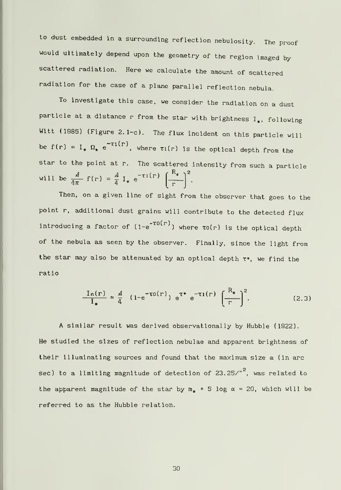
to dust embedded in a surrounding reflection nebulosity. The proof
would ultimately depend upon the geometry of the region imaged by
scattered radiation. Here we calculate the amount of scattered
radiation for the case of a plane parallel reflection nebula.
To investigate this case, we consider the radiation on a dust
particle at a distance r from the star with brightness I,, following
Witt (1985) (Figure 2.1-c). The flux incident on this particle will
be f(r) = I» e '^^^^\ where Ti(r) is the optical depth from the
star to the point at r. The scattered intensity from such a particle
will be ^f(r) = i T e-^^(-^'
471 4
Then, on a given line of sight from the observer that goes to the
point r, additional dust grains will contribute to the detected flux
introducing a factor of (l-e""^"^^^) where To(r) is the optical depth
of the nebula as seen by the observer. Finally, since the light from
the star may also be attenuated by an optical depth t», we find the
ratio
In(r) _ ^ -fo(r). T* -Ti(r)f^« f
A similar result was derived observational ly by Hubble (1922).
He studied the sizes of reflection nebulae and apparent brightness of
their illuminating sources and found that the maximum size a (in arc
sec) to a limiting magnitude of detection of 23.25/" , was related to
the apparent magnitude of the star by m^, + 5 log a = 20, which will be
referred to as the Hubble relation.
30
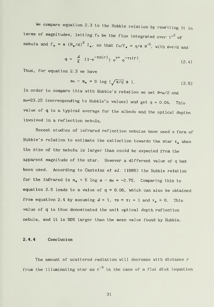
We compare equation 2.3 to the Hubble relation by rewriting it in
terms of magnitudes, letting fn be the flux integrated over l"^ of
nebula and f. = n (R,/d)^ I,, so that fn/f. = q/n e'^ with e=r/d and
q= t (l-e--(^))e-e--^^).
Thus, for equation 2.3 we have
mn - m, = 5 log (y n/q 9 ). (2.5)
In order to compare this with Hubble* s relation we set e=a/2 and
mn=23.25 (corresponding to Hubble' s values) and get q = 0.04. This
value of q is a typical average for the albedo and the optical depths
involved in a reflection nebula.
Recent studies of infrared reflection nebulae have used a form of
Bubble's relation to estimate the extinction towards the star when
the size of the nebula is larger than could be expected from the
apparent magnitude of the star. However a different value of q has
been used. According to Castelaz et ai. (1985) the Hubble relation
for the infrared is m, + 5 log a - mn = -2.75. Comparing this to
equation 2.5 leads to a value of q = 0.06, which can also be obtained
from equation 2.4 by assuming d = 1, to = ti = 1 and = 0. This
value of q is thus denominated the unit optical depth reflection
nebula, and it is 507. larger than the mean value found by Hubble.
2.4.4 Conclusion
The amount of scattered radiation will decrease with distance r
from the illuminating star as r in the case of a flat disk (equation
31
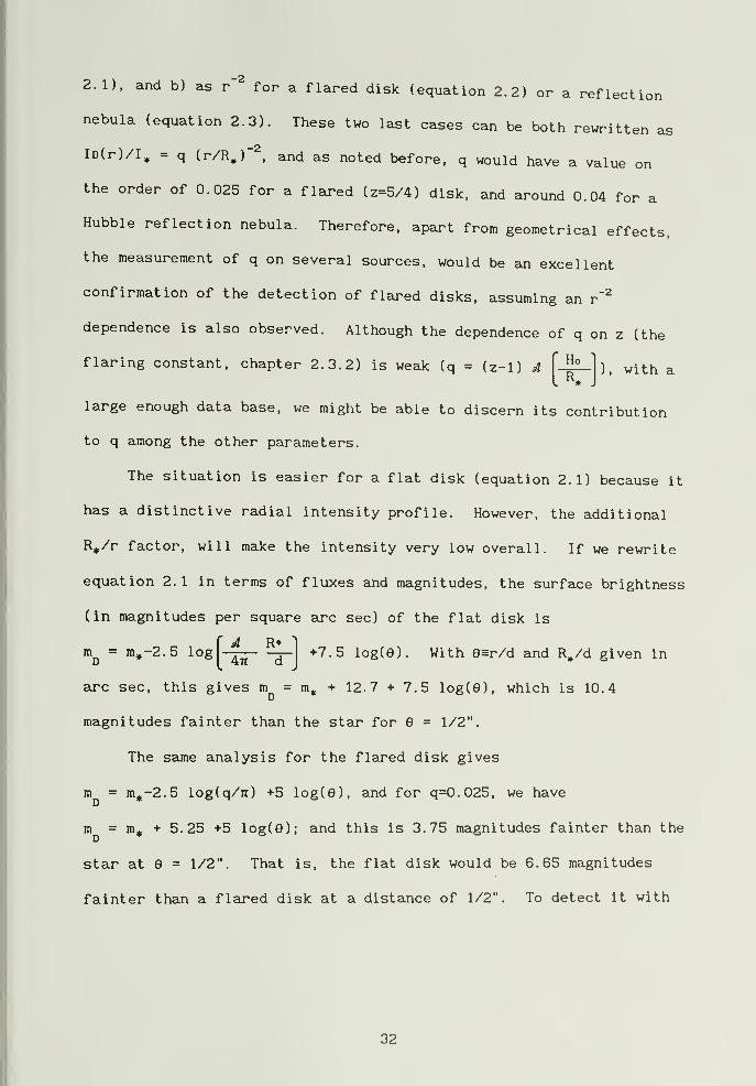
2.1). and b) as r" for a flared disk (equation 2.2) or a reflection
nebula (equation 2.3). These two last cases can be both rewritten as
lD(r)/I^ = q (r/R,)"^, and as noted before, q would have a value on
the order of 0.025 for a flared (2=5/4) disk, and around 0.04 for a
Hubble reflection nebula. Therefore, apart from geometrical effects,
the measurement of q on several sources, would be an excellent
confirmation of the detection of flared disks, assuming an r"^
dependence is also observed. Although the dependence of q on z (the
Ho) . with a
flaring constant, chapter 2.3.2) is weak (q = (z-1) ^
large enough data base, we might be able to discern its contribution
to q among the other parameters.
The situation is easier for a flat disk (equation 2.1) because it
has a distinctive radial intensity profile. However, the additional
R^/r factor, will make the intensity very low overall. If we rewrite
equation 2.1 in terms of fluxes and magnitudes, the surface brightness
(in magnitudes per square arc sec) of the flat disk is
= m,-2.5 log -^^^^ ^ +7.5 log(e). With e=r/d and R,/d given in
arc sec, this gives m^ = m, + 12.7 +7.5 log(e), which is 10.4
magnitudes fainter thaji the star for 9 = 1/2".
The s2une analysis for the flared disk gives
m^ = m^-2.5 log(q/7r) +5 log(e), and for q=0.025, we have
m = m, + 5.25 +5 log(9); and this is 3.75 magnitudes fainter than theD
star at e = 1/2". That is, the flat disk would be 6.65 magnitudes
fainter than a flared disk at a distance of 1/2". To detect it with
32
an equivalent signal to noise, would require a much larger (factor
~450) observing time.
Since most T-Tauri stars are intrinsically faint (because they
are low mass stars of late spectral type), and given that a flared
disk is most likely to be present (chapter 2.3.2). the observations
will be designed with the goal of detecting flared disks in as many
stars as possible, rather than searching for flat disks around a
single star.
33

34
CHAPTER 3
OBSERVATIONS
3.1 Introduction
The main purpose of this chapter is to justify the selected
observational procedure. We will show that it is in principle
possible to detect flared circumstel lar disks, and will calculate the
signal to noise expected in the observations. Finally, we will use
the calculation to define criteria in order to select objects to be
observed.
We begin with a justification for using infrared wavelengths.
Since star forming regions are still surrounded by residual gas and
dust, the use of infrared wavelengths is preferred because of they
suffer less extinction as we saw in chapter 2.4.1. The recent
development of infrared arrays of detectors facilitates the
possibility of imaging at these wavelengths.
In chapter 3.2 we will see the characteristics of the instrument
that was used. Spatial and temporal resolution of the instrument were
designed to be able to make speckle interferometric measurements. The
estimated signal to noise that can be attained with this system
(chapter 3.3) will provide a limiting magnitude of K~7.5 for the
objects that can be observed. This will be one of the selection
criteria. However, in addition we use the disk existence indicators
35
and the requirement that the object be close enough to be able to
resolve solar system size structures (chapter 3.4).
Our observations will be summarized in chapter 3.5 and a case
study of a good candidate, the YY-Ori star SCrA in the Corona
Australis dark clouds, will be discussed in chapter 3.6.
3.2 Instrumentation
In the past few years, technological advances have made possible
the integration of infrared detectors to form arrays. The Kitt Peak
National Observatory (KPNO) has recently developed an infrared speckle
system, based on such an array: a 58 by 62 pixel indium antimonide.
manufactured by Santa Barbara Research corporation. Among the nominal
features of this detector are: pixel size of 76x76 ^im; quantum
efficiency >80%; and 400 electron read-out noise (the dominant source
of noise at the K band). The control electronics and the optics were
developed at KPNO. The camera (Beckers et al. , 1988) in combination
with the KPNO 4m telescope and the f/28 secondary mirror, is capable
of providing different magnifications. We used optics that provide a
scale of 0.058" per pixel.
With this magnification, it is possible to achieve angular
resolutions up to the diffraction limit of the telescope (1.22 A/D
« 0.14" at 2.2 nm) . However, the atmosphere of the Earth blurres the
image of point sources to much larger sizes (~ 1" FWHM). However, the
use of such large magnifications is justified by the work of Labeyrie
36
(1970), who showed that during short exposures (smaller than than the
correlation time of the atmospheric variations that give rise to the
blurring), a photograph shows a speckled structure with frequency
components up to the diffraction limit. Correlation times up to a few
hundred milliseconds have been observed in the infrared. Several such
exposures may be combined together to increase the signal to noise in
a number of different ways like a) speckle interferometry, b)
centering to the center of mass and adding, or c) centering to speckle
locations and adding. There are deconvolut ion methods adequate to
each of these methods (chapter 4).
Some of these methods have been used successfully with
observations done using the system developed at KPNO, and diffraction
limited details are commonly recovered in objects brighter than 5
magnitudes in the K band.
The measured values for the performance of the system are a read
out noise of 9 counts per pixel and an efficiency of about 750 photons
(outside the atmosphere) per count at K.
3.3 Signal to Noise
The extent to which we can measure the flux attributed to the
disk will be limited by the noise associated with those measurements.
To identify a true signal from the disk above the background
noise for a single pixel, we require that the flux integrated over the
solid angle Qp subtended by that pixel and the period of time t, be
37
greater by a factor k (k usually equals 3 for a 3o- detection) than the
noise amplitude <r in that pixel. That is,
lD(e) fip t > k (T.(3
where IdO) is the intensity at a radial extent 9 in pixels from the
star.
Dividing this expression by f. = l^Q^ we have
f» t Qp lD(e)
- ^' (3.2)
which when combined with the expression for I for the flared disk
(equation 2.2) gives
f, t q^
0 ^ k. (3.3)
For a single exposure the noise will be signal independent and
dominated by the read out noise (cr =9 counts). For many exposures
(m), we would expect that the noise at a given pixel to increase as
the square root of m, if it were statistically independent. But we
will see (in chapter 4) that this is not the case, and that the
particular law for the increase of the noise will depend on the way in
which the frajnes are combined to produce an image or an
autocorre 1 at ion
.
However, to be able to make an estimate at this point, we will
assume that <r increases as while the signal f^^ increases as m, so
that after m frames of exposure time t we have
f, t qe"^ ^ k. (3.4)
38
This expression sets a limit for the maximum radial extent up to which
a flared disk can be detected, or alternatively the number of frames
needed to detect a disk up to a certain radial extent. If „e set this
distance to be 100 AU. that corresponds to 9 =11 pixels (for an object
150 PC away), we can construct a graph like Figure 3.1. This shows
the required number of frames to detect a flared disk of q=0.025 (see
chapter 2.4.3.2) for different fluxes of the star f, (in magnitudes at
K) and exposure times of 0.1 to 0.5 seconds. The shorter times are
better from the point of view of speckle interferometry. In fact, it
is unlikely that the correlation time of the atmosphere will exceed
0.3 seconds at K. Also, the performance of the system is such that
only ~2 frames per second can be obtained independently of the
integration time, thus adding to the total observing time for a large
number of frames. Long term atmospheric variations made us choose
-500 frames as the maximum. With these estimates, the maximum
magnitude that can be observed doing speckle work is 6.5 at K. For
image centering, larger integration times may be chosen, but in order
to suppress image motion this should be kept under 1 second (unless an
automatic guider is in use), and so a ma>cimum magnitude of K~7.5 seems
appropriate. Since it is not uncommon for T-Tauri stars to show
variations in intensity of half a magnitude, an upper limit of K~8
will be used in the next chapter to generate a list of candidates for
observation.
39
3.4 Object Selection
A list of T-Tauri stars to observe can be generated by ussing
three basic criteria: that the object be a) bright enough to be able
to observe a flared disk (K<8) with the KPNO IR speckle camera; b)
that it have disk existence indicators (Far Infrared emission); and
finally, c) that it be near enough that a disk of solar system
dimension may be resolvable.
Three nearby clouds (d~150pc) with known ongoing star formation
(cf. Shu, Adams, and Lizano, 1987) were selected. The Taurus cloud
complex is the one that has been most extensively studied. It is
knovm to have a relatively low density and efficiency of star
formation, and is probably dominated by magnetic fields (subcritical )
.
The p-Ophiuchus and R Corona Austral is are more obscured regions, with
higher star formation efficiencies. They are probably gravitational ly
dominated (supercritical) and forming bound clusters.
Near infrared (NIR) photometry for stars in the Taurus clouds has
been carried out by a number of workers over the past 15 years (cf
.
Strom et al. , 1989). Furthermore, the Infrared Astronomical Satellite
(IRAS) made far infrared (FIR) measurements at 12, 25, 60 and 100 ixm
and has allowed identifications with the known young stellar objects.
Strom et al. (1989) have compiled the photometry at these wavelengths
8Lnd have thereby identified the passage from an active inner disk (r
<0. 1 AU) to a depleted inner disk on the basis of the emission excess
at K (NIR). From this they set an age of 3x10 years for the
40
transition. However, the outer portions of the disk are still present
until the FIR emission disappears. In table 3.1 we list the objects
with K <8 and FIR emission identified as either T-Tauri stars or Weak
T-Tauri stars in Strom et ai. (1989). We list for each object the NIR
magnitudes (J, H. K. L), the IRAS fluxes (12. 25 60, 100 ^m) in Jy,
and an estimate of the spectral index n given by the ratio of fluxes
at 25 and 12 Mm, that is, n = 1 - log( I25/I12)log(25/12)
NIR surveys of the p-Ophiuchus dark clouds have been done by
Grasdalen et al. (1973). Vrba et al. (1975), Elias (1978), Wilking and
Lada (1983). Lada and Wilking (1984) classified the spectral energy
distributions (in NIR and MIR) of the objects in terms of the spectral
index, and noted that many of the stars that had been previously
classified as early spectral types (A and B). were really T-Tauri
stars with large (intrinsic) infrared excesses.
Young, Lada, and Wilking (1986) (YLW) identified a number of IRAS
sources in a small central region of the cloud, by performing mid
infrared observations (10 y.m) from a ground based observatory (IRTF)
in order to compare with the IRAS fluxes at 12 nm. However, sources
in a large portion of the cloud remain unidentified at these
wavelengths. For our studies, we present in table 3.2 a possible
identification of some of the objects associated with the cloud in the
list of Elias (1978) with K <8. that are not in the region surveyed by
YLW, to IRAS sources closer than ~1' to the star, taJcen from the IRAS
Point Source Catalog. This identification should be taken only as an
indication of the possibility of existence of FIR emission. Many of
41
the sources thus identified, show an incredibly large flux (GSS25.
GSS30, GSS31. and GSS35), while others (S-R4, EL24. S-R9 and MWC863)
show plausible values.
In table 3.3 we present the list of objects with K <8 taken from
Elias (1978) and Wilking and Lada (1983) that have either confirmed
(YLW) or possible (table 3.2) FIR emission.
In the R era region, NIR photometry by Knacke et al. (1973) and
Vrba et al. (1976) provides us with only two sources with K <8 that
are listed in the IRAS Point Source Catalog and which definitely have
FIR emission as well. These are given in table 3.4.
3 . 5 Observat ions
We were granted observing time in some of the first runs with the
KPNO new IR speckle system during 4 nights in February and 3 nights in
May of 1989, for the purpose of detecting disks around young stars.
People involved in those observations were Steve Ridgway, Julian
Christou, Dave Weintraub, Hanz Zinnecker, 8ind myself. The observing
time was shared between this project and others, such as observations
of circumstel lar shells around old stars and young binary stars.
The selected mode of operation was to taJce a set of a few hundred
short exposures (100 ms to 1 s), in order to make it possible to
increase the angular resolution via speckle interferometry or image
motion suppression. Our observations were haunpered because the
42

automatic guider could only be used during the February run, due to a
malfunction in May.
Each observation of an object consisted of 128 to 512 short
exposures. Table 3.5 gives a list of the objects observed during
these two periods listing name (most common in the case of p-Oph
sources) and association, date observed, filter, number of
observations, integration time per exposure, and number of exposures
per observation.
Stars from the SAO catalog, slightly brighter than the object,
were used as calibrators for the PSF. K magnitudes were estimated
from the V magnitudes and the spectral type. Observations of the
object, sky, and PSF standards were interleaved. Table 3.6 lists the
reference stars used for each of the objects.
On the basis of these observations we have chosen SCrA as a case
study and will describe it below in some detail.
3.6 SCrA as a Case Study
There are several reasons to choose SCrA as a case study.
1) It belongs to the YY-Ori sub-class of T-Tauri stars and hence
it is believed to be in the a state of active accretion of material
from a disk onto the star. The term YY Orionis star was introduced by
Walker in 1961 (see Walker, 1972) to denote T-Tauri stars with
unusually strong ultraviolet excess and redward displaced absorption
lines, indicative of infall of material, at velocities -300 Km/s.
43
The YY-Ori character of SCrA was discovered by Appenzeller and
Wolf (1977) (AW77). and it was identified to be the brightest star of
its kind yet observed. Further observations of SCrA have shown that
the profiles of forbidden lines in emission like [Oi] and [Sii], are
very similar to those of normal T-Tauri stars (Strom, Strom and
Edwards, 1987), that is they are only blueshifted, indicating the
presence of an obscuring screen or disk at large distances from the
star (see chapter 2.2.2).
The Balmer series of Hydrogen in SCrA shows the standard P-Cygni
III profile at Ha. with blueshifted as well as redshifted emission and
absorption at rest velocity, indicative of a bipolar outflow at
distances of tens of R^. But higher transitions in the series (H^,
Hy, H5) show the development of a redshifted absorption component,
indicative of infall onto the star at distances closer to the star's
surface (Edwards, 1979; AW77).
2) It is a binary star with separation 1"37 and so provides a
good way of comparing the results for the two stars simulteineously.
The companion was about 1 magnitude fainter in 1981 and its located at
PA 147 . According to AW77, it also seems to have similar spectral
characteristics to the main star (T-Tauri like).
3) Speckle observations in visible wavelengths have been done by
Dr. Pete Nisenson (at CFA), and analyzed by him. So we can compeu^e
our results and methods with his.
4) The set of our IR observations consists of 5 observations on
SCrA and 4 on a close reference star (SAO 210781), each with 256
44
frames of 200 ms integration time showing speckle structure. The
observations of the reference were interleaved with those of SCrA and
measurements of the sky intensity. In particular for 3 of the
observations, the reference star occupied the exact same position in
the sky than the next observation of SCrA. This may turn out to be
important if deformations in the structure of the telescope causing
aberrations are due to gravity.
45
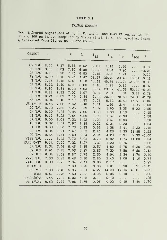
TABLE 3.1
TAURUS SOURCES
Near infrared magnitudes at J, H. K, and L. and IRAS fluxes at 12 2560 and 100 ^xm in Jy. compiled by Strom et al. 1989; and spectral indeiT) estimated from fluxes at 12 and 25 /im.
OBJECT J H K L I I T t12 '25 ^60 ^00
CW TAU 9. 00 7. 87 6. RR K*J .
RP od.
.
C 1 4. 1 A14 3. 56 0. 37DD TAU 9. 56 8. 62 7, 97 RR n PT oJ
.
C A5. 90 -2. 76
DE TAU 9. 15 8. 26 7_ 711 J. nu
.
A Q'its U . oU 1
.
21 0. 30RY TAU 8. 00 6. 78 5. 74. A 1 Q A V on '7n
/ y 20. 48 15. 91 0. 42T TAU 7. 15 6. 18 5. 40 A 1 R ID .
A Q A Q bb 111. 74 121
.
85 -0. 50DF TAU 8. 32 7. 40 6. RlO 1
c;o
.
RQ 11
.
1 RID 1
.
oo0. 65 0. 87
DC TAU 8. 96 7. 81 6. 73 o .1 n R/1 pp oy A 141
.
by 53. 13 -0. 08DK TAU 8. 88 7. 82 7. 03 5. 97 P4. c,
.
R/li .
R /Ib4 J
.
67 0. 78HL TAU 10. 21 8. 67 7. 10 5. 34 7 R4. PQ^y
.
Uo / u
.
Rn •7 A1 4 . bU -0
.
79XZ TAU 9. 34 8. 16 7. 17 5. 85 r> 3R R RP 1 RID .
Rn 1 v1 / .
Rr\bU U .
f\ A04UZ TAU E 8. 45 7. 60 7. 02 6. 40 1
.
51 1X . Q1 p /1
1
11 .PRcb U
.
ROboGG TAU 8. 79 7. 85 7. 25 6. 39 1
.
37 1X •oo
.
PR RD .np n RR
, bbGH TAU 9. 30 8. 38 7. 86 7. 05 0. 69 1X I 03 1X .
1 R, X o * '
n A R. 4D
GI TAU 9. 16 8. 22 7. 55 6. 60 1. 23 1
.
67 n 9R nu
,
RQ. Oo
GK TAU 9. 00 8. 01 7. 32 6. 42 1
.
. 23 1 R7 n u
,
RQ
IS TAU 9. 52 8. 51 7. 97 7. 19 0.,32 0.,31 0..20 . .. . . 1 .04Li 1 AU a. bO 8. 50 7. 76 6. 83 0., 92 1.. 38 2 , 41 2.. 32 0 .45HP TAU 9. 34 8. 24 7. 47 6. 52 2.,41 4..26 8,.33 21..86 0 .22DO TAU 9. 64 8. 44 7. 49 6. 24 2..04 4,.26 6 .91 7,.95 -0 .00
V955 TAU 8. 42 7. 73 6. 93 0..73 0..82 1 .74 11,.00 0 .84HARO 6-37 9. 14 7. 99 7. 23 6. 27 1,.20 1..20 0 .79 1 .00
DR TAU 8. 54 7. 46 6.,45 5. 15 3.,57 4..80 5,.76 6,.20 0 .60UY AUR 8. 91 7. 85 7. 05 5. 87 3..85 7,.30 7 .89 6 .80 0 . 13
RW AUR 8. 54 7. 62 6. 87 5. 79 2..60 4,.04 3 .34 1,.70 0 .40V773 TAU 7. 63 6. 83 6. 48 5. 86 2..80 3..40 2 .00 1,. 10 0 .74
V410 TAU 8. 33 7. 73 7.,54 7. 41 0,.90 0., 17 3 .27
UX TAU A 7. 58 6. 98 0..30 1,.81 3 .90 5,.51 -1 .45
SU AUR 7. 03 6.,46 5.,95 5. 21 4,.27 14..30 17,. 16 43,.61 -0 .65
LkCa3 8. 47 7.,76 7.,53 7. 32 0..05 0..05 0 . 10 1 .00
HDE283572 7. 46 7.,04 6.,93 6. 85 0.. 11 0.. 19 0 .26
Wa TAU/1 8. 52 7.,99 7., 85 7. 76 0,.05 0..03 0 . 10 1 . 40 1 .70
46
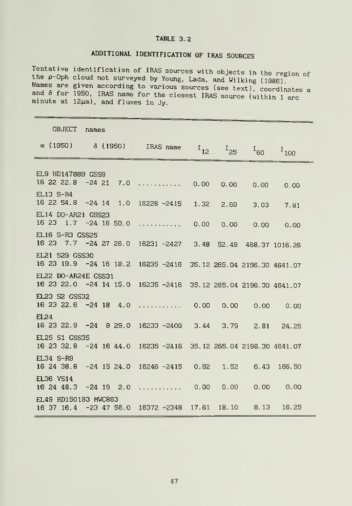
TABLE 3.2
ADDITIONAL IDENTIFICATION OF IRAS SOURCES
Tentative identification of IRAS sources with objects in the region ofthe p-Oph cloud not surveyed by Young. Lada, and Wi Iking (1986)Names are given according to various sources (see text), coordinates aand 6 for 1950. IRAS name for the closest IRAS source (within 1 arcminute at 12/im), and fluxes in Jy.
OBJECT names
a (1950) 8 (1950) IRAS name I I I t12 '25 ^60 SoO
EL9 HD147889 GSS916 22 22.8 -24 21 7.0 0.00 0.00 0.00 0.00
EL13 S-R416 22 54.8 -24 14 1.0 16228 -2415 1.32 2.69 3.03 7.91
EL 14 D0-AR21 GSS2316 23 1.7 -24 16 50.0 0.00 0.00 0.00 0.00
EL16 S-R3 GSS2516 23 7.7 -24 27 26.0 16231 -2427 3.48 52.49 468.37 1016.26
EL21 S29 GSS3016 23 19.9 -24 16 18.2 16235 -2416 35.12 265.04 2196.30 4641.07
EL22 D0-AR24E GSS3116 23 22.0 -24 14 15.0 16235 -2416 35.12 265.04 2196.30 4641.07
EL23 S2 GSS3216 23 22.6 -24 18 4.0 0.00 0.00 0.00 0.00
EL2416 23 22.9 -24 9 29.0 16233 -2409 3.44 3.79 2.81 24.25
EL25 SI GSS3516 23 32.8 -24 16 44.0 16235 -2416 35.12 265.04 2196.30 4641.07
EL34 S-R916 24 38.8 -24 15 24.0 16246 -2415 0.92 1.52 6.43 166.50
EL36 VS1416 24 48.3 -24 19 2.0 0.00 0.00 0.00 0.00
EL49 HD 150 193 MWC86316 37 16.4 -23 47 56.0 16372 -2348 17.61 18.10 8.13 16.25
47
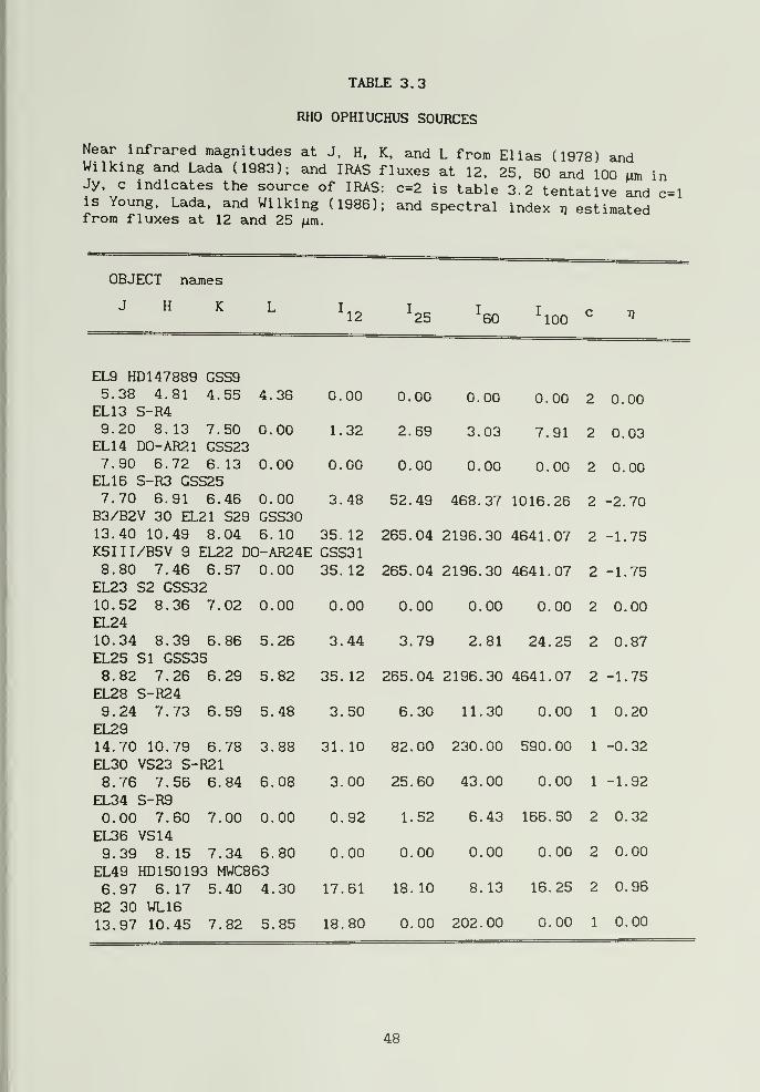
TABLE 3.3
RHO OPHIUCHUS SOURCES
Near infrared magnitudes at J, H, K, and L from Elias (1978) andWilking and Lada (1983); and IRAS fluxes at 12, 25, 60 and 100 im inJy, c indicates the source of IRAS: c=2 is table 3.2 tentative and c=lIS Young. Lada. and Wilking (1986); and spectral index d estimatedfrom fluxes at 12 and 25 fxm.
OBJECT names
J H K L I12
I25
I60 ^100 c 7)
EL9 HD147889 GSS95.38 4.81 4.55 4. 36 0. 00 0. 00 0. 00 0. 00 2 0. 00
EL13 S-R49.20 8.13 7.50 0. 00 1. 32 2. 69 3. 03 7. 91 2 0. 03
EL14 D0-AR21 GSS237.90 6.72 6.13 0. 00 0. 00 0. 00 0. 00 0. 00 2 0. 00
EL 16 S-R3 GSS257.70 6.91 6.46 0. 00 3. 48 52. 49 468. 37 1016. 26 2 -2. 70B3/B2V 30 EL21 S29 GSS3013.40 10.49 8.04 6. 10 35. 12 265. 04 2196. 30 4641. 07 2 -1.,75
K5III/B5V 9 EL22 D0-AR24E GSS318.80 7.46 6.57 0. 00 35. 12 265. 04 2196. 30 4641. 07 2 -1,.75EL23 52 GSS3210.52 8.36 7.02 0. 00 0. 00 0. 00 0. 00 0.,00 2 0,.00EL2410.34 8.39 6.86 5. 26 3. 44 3. 79 2. 81 24,,25 2 0 .87
EL25 SI GSS358.82 7.26 6.29 5. 82 35. 12 265. 04 2196. 30 4641.,07 2 -1 .75
EL28 S-R249.24 7.73 6.59 5. 48 3. 50 6. 30 11. 30 0.,00 1 0 .20
EL2914.70 10.79 6.78 3. 88 31. 10 82. 00 230.,00 590..00 1 -0 .32
EL30 VS23 S-R218.76 7.56 6.84 6. 08 3. 00 25. 60 43.,00 0,.00 1 -1 .92
EL34 S-R90.00 7.60 7.00 0. 00 0. 92 1. 52 6.,43 166,.50 2 0 .32
EL36 VS149.39 8.15 7.34 6. 80 0. 00 0. 00 0.,00 0 .00 2 0 .00
EL49 HD 150 193 MWC8636.97 6.17 5.40 4. 30 17. 61 18. 10 8., 13 16,.25 2 0 .96
B2 30 WL1613.97 10.45 7.82 5. 85 18. 80 0.,00 202.,00 0 .00 1 0 .00
48
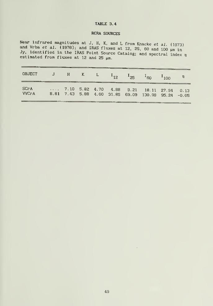
TABLE 3.4
RCRA SOURCES
Near infrared magnitudes at J, H, K. and L from Knacke et al (1973)and Vrba et al. (1976); and IRAS fluxes at 12. 25, 60 and 100 urn inJy. identified in the IRAS Point Source Catalog; and spectral indexestimated from fluxes at 12 and 25 iim.
OBJECT J H K L l2 25 so ^100 V
SCrAVVCrA
7.108.81 7.43
5. 825.88
4.704.00
4.8831.85
9.2169.09
18. 11
130.9927.9495.24
0. 13
-0.05
49
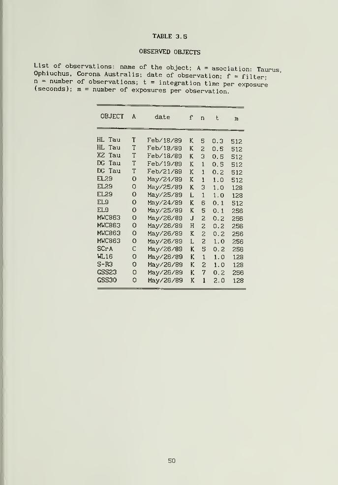
TABLE 3.5
OBSERVED OBJECTS
List of observations: name of the object; A = asociation- TaurusOphiuchus, Corona Austral is; date of observation; f = filter-n = number of observations; t = integration time 'per exposure(seconds); m = number of exposures per observation.
OBJECT A \Ji<X C C cI n t m
HL Tau T Pp^Vi/l Q /QQ O U. J 512HL Tau T1 P /QQ V
Pk U. O 512XZ Tau T r c u/ io/ OiD V o U
.
O blii
DG Tau T 1 U
.
cO C 1 oOlii
DC Tau T 1X U.
EL29 0 May/24/89 K 1 1. 0 512EL29 0 May/25/89 K 3 1. 0 128EL29 0 May/25/89 L 1 1. 0 128EL9 0 May/24/89 K 6 0. 1 512EL9 0 May/25/89 K 5 0. 1 256MWC863 0 May/26/89 J 2 0. 2 256MWC863 0 May/26/89 H 2 0. 2 256MWC863 0 May/26/89 K 2 0. 2 256MWC863 0 May/26/89 L 2 1.,0 256SCrA c May/26/89 K 5 0,,2 256WL16 0 May/26/89 K 1 1,,0 128S-R3 0 May/26/89 K 2 1,,0 128GSS23 0 May/26/89 K 7 0,.2 256GSS30 0 May/26/89 K 1 2 .0 128
50
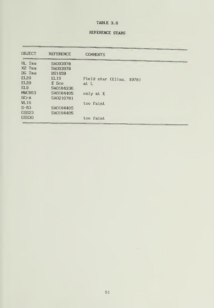
TABLE 3.6
REFERENCE STARS
OBJECT REFERENCE COMhENTS
HL Tau SA093978XZ Tau SA093978DG Tau BS1459EL29 EL15 Field starEL29 Z Sco at LEL9 SA0184336MWC863 SA0184405 only at KSCrA SA02 10781WL16 too faintS-R3 SA0184405GSS23 SA0184405GSS30 too faint
51
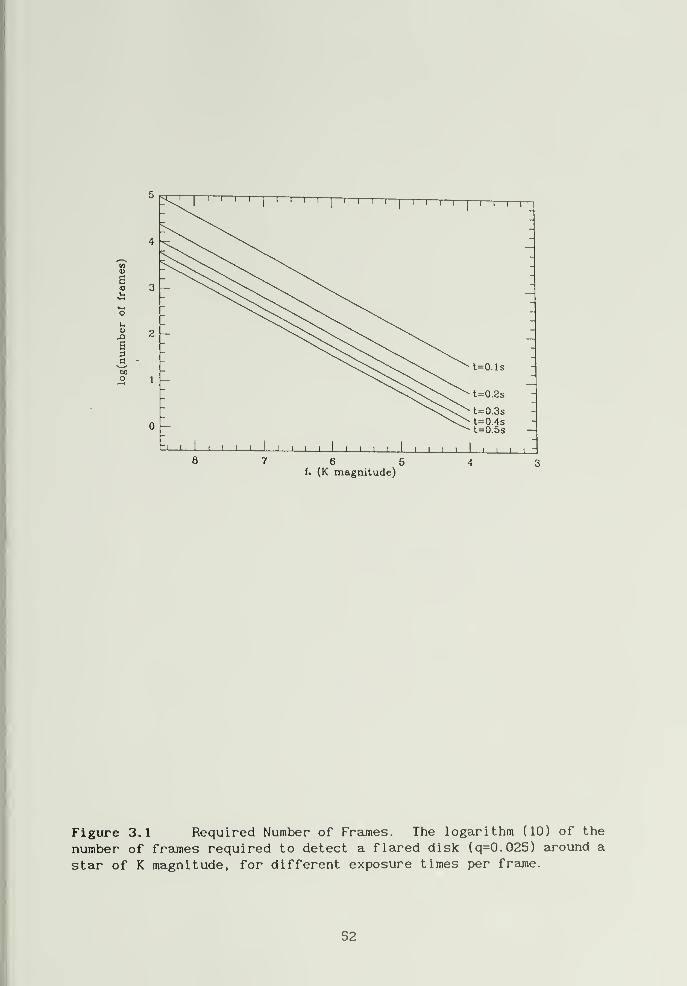
8 7 6 5f. (K magnitude)
4 3
Figure 3.1 Required Number of Frajnes. The logarithm (10) of the
number of frames required to detect a flared disk (q=0.025) around a
star of K magnitude, for different exposure times per frame.
52
CHAPTER 4
DATA ANALYSIS
4.1 Introduction
The main concern in analysing the obtained images is to separate
the response of the imaging system from the real features of the
object, within the limits allowed by the noise inherent in the
observations. A critical part of this noise arises from the earth's
atmosphere and the telescope, so we begin in chapter 4.2 by discussing
the image formation process and the expected contributions of the
earth's atmosphere and the telescope's optics to that response.
This introduction will provide us with an expected appearance for
the images that we have obtained. But the data is not initially in
the form of images. Observations consist of single frames with short
exposure times. A series of tasks have to be performed initially on
those frames (chapter 4.3) to remove contributions due to the
electronics and the optics of the system.
From there on, we can divide the different analysis methods in
three categories depending on the way in which we combine the frames
to produce an image. They can be either a) directly averaged (with
proper centering) thus producing the equivalent of a longer exposure
image; or b) the speckle nature of each frajne can be exploited to
produce a diffraction limited image; or finally c) the analysis can be
carried out in frequency space rather than in image space via speckle
interferometry. These methods will be analyzed in sections 4.4
53
through 4.6 under the names of Center and Add. Speckle Shift and Add.
and Speckle Interferometry.
Each of these methods has its advantages as well as its
drawbacks. In particular, all of them require some sort of
deconvolution of the instrumental response or Point Spread Function
(PSF). to distinguish features in the final image that are due to the
observing process from those due to the object itself. At this stage
the analysis can take several directions to deconvolve the PSF using
different algorithms.
We will apply each of the methods developed here to the
observations done on the star SCrA. Although we will be able to see
effects approximately as expected for a flared disk, we will find that
the response function of the telescope as a major problem in getting
conclusive results.
4.2 Image Formation Basics
The process by which images are formed in a linear optical system
can be described by the equation
I(x) = P(x) * 0(x), (4.1)
which relates the intensity I(x), measured at each position x in the
image plane, to the object 0(x), by its convolution with the Point
Spread Function (PSF) P(x). This equation is valid in a limited
region (in x) known as the isoplanatic patch, where the PSF is
invariant under translations. Its size has been measured to be on the
order of 20" in optical telescopes (Roddier, 1981). This value is
54
much larger than the field of view of the KPNO IR camera which is
3.5", so the issue of isoplanaticity will not be further addressed.
Our goal is to find 0(x) from the observed l(x). To do this we
must first determine the PSF. The PSF. however, is set by the optical
system and the atmosphere. Thus we shall considere each part
sepaj^ately.
4.2.1 Telescope Contribution
The PSF is the response of the optical system to an impulse. In
the case of a telescope, the PSF can be measured by looking at an
unresolved star. Stars, being self luminous, are considered to be
incoherent sources of radiation, and the telescope itself as a system
linear in intensities. Hence, according to Born and Wolf (chapter 9,
1959), the Fourier transform of the PSF, P(u), where u denotes spatial
frequency, is the autocorrelation of the pupil function H(u),
P(u) =J
H(u') H(u'-u) du'. (4.2)
The puil function H(u) is a window function that maps the aperture
(given by the main mirror in a telescope), while the spatial frequency
u is linearly related to the position in the main mirror ^, and the
space spajined by these coordinates is the Fourier transform space of
the image space.
For a circular aperture, as in the case of a telescope, H(u) is
simply a window function that is 1 inside the aperture (u < (A/D) ^)
and 0 outside of it. The PSF is then given by the inverse Fourier
trajisform of equation (4.2), giving rise to a combination of Bessel
55
functions that generate an Airy pattern (see Born and Wolf, chapter 8.
1959). The effect of a central hole can be included as well, and in
the case of aberrations, the pupil function is a complex quantity.
The effect of the atmosphere of the earth in the propagation of
an initially plane wave can be included in the pupil function by
H(u) = Ho(u) S(u), (4 3)
where Ho denotes the telescope and S the atmospheric contribution. As
a consequence of this, it is not in general trivial to separate the
contribution of the telescope from that of the atmosphere in equation
4.1 due to equation 4.2. Furthermore, real data is affected by the
presence of noise N(x) so that equation 4.1 should really be written
Kx) = P(x) » 0(x) + N(x). (4.4)
4.2.2 Atmospheric Contribution
The blurring that the atmosphere of the earth introduces in
astronomical images is usually the main limitation in high resolution
imaging because the size of the blurred image is This blurring
occurs as electromagnetic waves propagate through a turbulent medium
with varying index of refraction causing distortions (phase
variations) in the wavefront as well as image motion (wavefront tilt).
The contribution of these processes to image degradation is well
understood from a theoretical point of view, and has been corroborated
experimentally (see review by Roddier, 1981). Their effects on the
PSF will be summarized in chapter 4.2.3. However, single images taken
with short exposure times are dominated by a random pattern of bright
56
speckles that resemble a bunch of grapes. This phenomena will be
addressed in chapter 4.2.4.
4.2.3 Long and Short Exposures
Fried (1966) described the effect of the atmosphere in blurring
the image of a star with a single number ro, related to the seeing
FWHM Z by Z = X/ro,. This is the correlation length of the atmosphere
(see also Roddier. 1981) which is approximately 45 cm for 1" seeing at
A=2. 2;im.
For a large telescope of diameter D > ro, a long exposure image
is degraded by turbulence in the atmosphere. Fried (1966) has shown
that the Fourier transform of the mean PSF, <P(u)>, can be separated
in a telescope component t(u) (assumed constant) and an atmospheric
component B(|u|), where |ul denotes the norm of the two dimensional
vector u of spatial frequencies. Thus, we caji write
<P(u)> = T(u) B( |u| ). (4.5)
For our study, we take
B(|u|) = exp(-3.44 (X |u|/ro)^^^), (4.6)
following the model of Fried (1966) and let f(u) be given by the
autocorrelation of the telescope pupil's function Ho(u) (as equation
4.2). The 5/3 exponent comes from Kolmogorov's theory of turbulence
(1941), which asserts that in turbulent motion, the kinetic energy is
transferred to smaller and smaller scales.
With f (u) and B(u) specified, we can now find the PSF, P(x) by
taking the two dimensional inverse Fourier transform, or for circular
57
symmetry of T(u). the Inverse Hankel transform of equation 4.5. The
function P(x) so defined Is very similar to a gausslan In the core
(0 < 2<r, es|x|) but falls off less steeply, at a rate o'^ with p~4.
This behavior explains the data published by King (1971) for the
profiles of stellar Images.
Although the seeing parameter can be too large for our purposes
(Z-l"), a significant Improvement (factor of 1.5) should be achievable
by reducing the Image motion component of the long exposure PSF,
either by using a fast automatic gulder or by shifting short exposure
frames to their center of mass and adding. However, In this case
B(|u|) follows a modified Kolmogorov spectrum such that
B(|u|) = exp(-3.44 (A \u\ /vof^^ {\-{\ |u|/D)'^^) ). (4.7)
and the resultant PSF Is Fried' s "short exposure PSF" (Fried, 1966).
In Figure 4.1 we show the expected radial profiles of the PSF at
\ =2.2^im, calculated from the inverse Fourier transform of equation
4.5, for both short and long exposures, and for values of ro from 30
cm to 80 cm. As it can be seen from Figure 4. 1-a, the width of the
short exposure profile is always smaller (-2/3) than that of the long
exposure; the central core resembles a gausslan better for the long
exposure than for the short one (Figure 4.1-c), and the fall off in
the wings (Figure 4. 1-b) is more pronounced (corresponding to a power
law wlht p ~ -4) for the long exposure than for the short exposure (p
~ -3.3).
58
4.2.4 Speckle Phenomena
Long and short exposure PSF' s represent an average situation for
the behavior of the PSF. However, single frames taken with short
exposures present a different structure, a transient. Images in short
exposure frames are therefore characterized by an atmospheric induced
seeing spot interior to which is a random pattern of bright speckles.
Labeyrie (1970) suggested that speckle grains can be identified
with the coherence domains of the Bose-Einstein statistics. That is,
photons as spin 0 indistinguishable particles, tend to bunch together
in each energy state. Although this interpretation has not been
refuted, another one, by Korff. Dryden, and Miller (1972) (KDM), is
more accepted. In the KDM theory, cells of size ro in the atmosphere
produce random phase and amplitude variations to the incoming
wavefront, and the resulting intensities in the image are the result
of coherent superposition, in accordance with a two dimensional random
walk problem.
Following KDM, the characteristic size of each speckle is given
by the diffraction limited central spot of the Airy pattern of the
telescope aperture. Since the radius to the first zero Airy ring is
~ A/D (the actual factor depends on the amount of central obscuration
in the aperture due to the hole in the main mirror, but it is always
close to 1), we have that the mean separation between speckles is
~ 2 A/D.
For our infrared observations: A=2.2/im. D=4m, and with a scale
plate of 0. 058"/pixel , the mean separation between speckles is 0"22 or
59
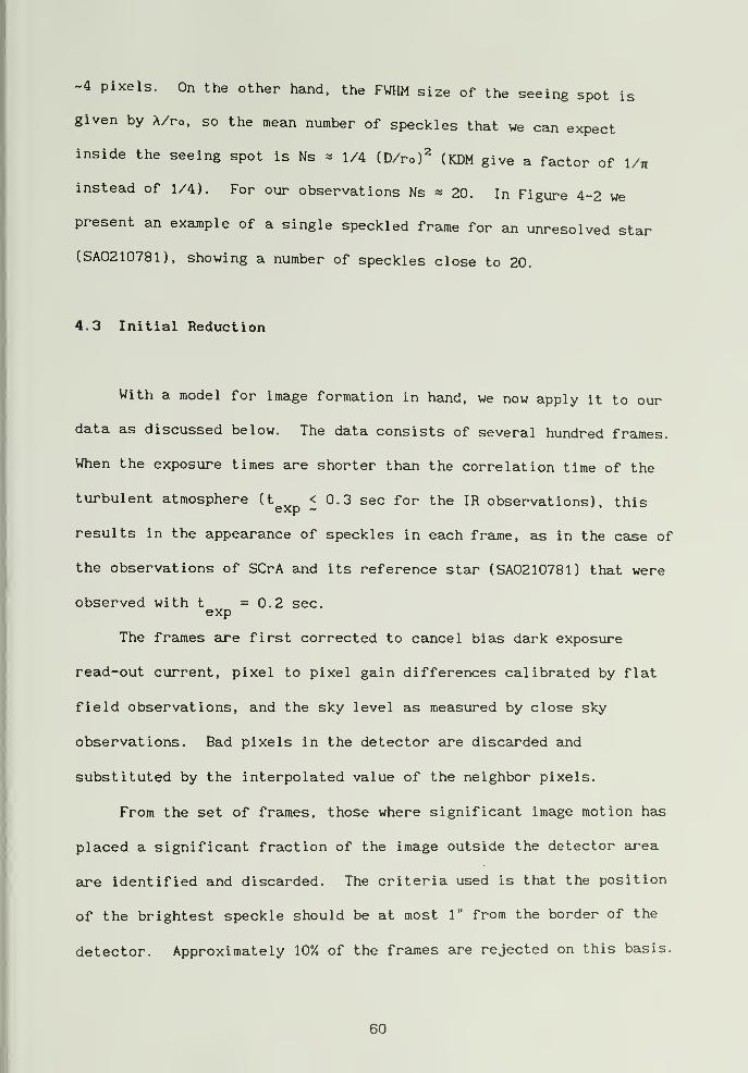
-4 pixels. On the other hand, the FWHM size of the seeing spot is
given by X/ro, so the mean number of speckles that we can expect
inside the seeing spot is Ns ^ 1/4 (D/ro)^ (KDM give a factor of 1/n
instead of 1/4). For our observations Ns « 20. In Figure 4-2 we
present an example of a single speckled frame for an unresolved star
(SA0210781), showing a number of speckles close to 20.
4.3 Initial Reduction
With a model for image formation in hand, we now apply it to our
data as discussed below. The data consists of several hundred frames.
When the exposure times are shorter than the correlation time of the
turbulent atmosphere (t^^^ ^ ^.3 sec for the IR observations), this
results in the appearance of speckles in each frajne, as in the case of
the observations of SCrA and its reference star (SA0210781) that were
observed with t =0.2 sec.exp
The frames are first corrected to cajicel bias dark exposure
read-out current, pixel to pixel gain differences calibrated by flat
field observations, and the sky level as measured by close sky
observations. Bad pixels in the detector are discarded and
substituted by the interpolated value of the neighbor pixels.
From the set of frajnes, those where significajit image motion has
placed a significant fraction of the image outside the detector area.
are identified and discarded. The criteria used is that the position
of the brightest speckle should be at most 1" from the border of the
detector. Approximately 10% of the frames are rejected on this basis.
60
Alternatively, when the exposure times are longer than the correlation
time of the atmosphere so that there are no speckles present, the
criteria used is that the total power detected in each frame should
not deviate from the mean by more than 2 standard deviations.
4.4 Center and Add Method
In order to get the equivalent of a short exposure integrated
image (chapter 4.2.3). we have to calculate the center of mass in each
frame, shift all frames to the same center, and add. This compensates
for image motion due to changes in the wavefront directions induced by
the turbulent atmosphere, and also those due to poor guiding of the
telescope. We will show that finding the center of mass with the
required accuracy (section 4.4.1) is not a problem for most of the
observations. As an example, center and add images for SCrA and its
reference star were obtained, and the radial profiles of the response
compared to the expected short exposure profiles (section 4.4.2). The
results are ambiguous as we shall see.
To decide if it is possible to detect a flared disk around SCrA,
we will analyze the noise present in the center and add images
(section 4.4.3), noting some interesting behavior. Later, we conclude
that there is enough signal-to-noise to detect the disk by means of
the contrast ratio of its intensity to the PSF. which is on the order
of 10% (section 4.4.4), assuming that the disk is resolved. A
structure of the required intensity can be observed, but as we will
see, a lack of stability in the response function of the telescope
61
produces effects of comparable magnitude. In section 4.4.5 .we will
present a description and analysis of the response function of the
telescope separated from that of the atmosphere by means of a maximum
entropy criteria and conclude that it has random components that vary
by 307. typically.
In section 4.4.6 we will relax the assumption that the disk is
resolved, and try to deconvolve the PSF. The maximum entropy criteria
will prove insufficient to recover high contrast structures with the
amount of noise present, apart from the differences in the response of
the telescope. A recently developed blind deconvolut ion algorithm is
more promising for the case in which the response of the telescope is
not known. However, its behavior is chaotic in the presence of noise.
4.4.1 Frame Centering
The accuracy with which we caji determine the center of mass of
each frame is important because errors may cause additional dispersion
in the width of the PSF, and thus be erroneously interpreted as a real
extension of the object.
The position of the x coordinate of the center of mass xc is
N N
given by X = -4— \ ) x d , where d is the observed flux at^ iJ 'J 'J
j=i 1=1
position X and d is the total flux in the N by N box. The^ ij T
2 —N o- -
uncertainty in this position is 5x = , where <r is the meain
2 V3 dT
noise in the data, <r . We can take a- to be the amplitude of the
62
read-out noise (9 counts), which is the dominant source of noise at K
for a single frame. Now for the IR detector. N^=60x60 pixels, and for
the observations on SCrA, d^ =19000 counts, so Sx^ =0.5 pixels. When
adding many frames together, this uncertainty will introduce a very
small (<1%) dispersion in the width of the PSF. and thus it is not
necessary to restrict the size of the box to calculate the center of
mass.
The result of the frame centering procedure is shown in Figure
4.3 for the binary star SCrA and its reference star, obtained by
processing the 256 exposures of one typical observation.
4.4.2 Radial Profiles
A comparison of the radial profiles obtained by the center and
add method with the expected theoretical short and long exposure
profiles (chapter 4.2.2 and Figure 4.1) is presented in Figure 4.4. A
successful comparison should test the hypothesis that a significaiit
improvement in the FWHM can be obtained by removing the image motion
component of the seeing.
The radial profiles of the reference star (for SCrA) are obtained
by averaging all azimuthal contributions at each radial position from
the center of mass. Up to a radial distance of 15 pixels (0.9") the
profile is better represented by a short exposure profile with ro =33
cm. implying a seeing of Z =X/ro = 1.37". But from there up to 25
pixels (1.45") it can be best described as a long exposure with ro =47
cm. and with an associated I =0.96". The measured FWHM is more like
63
0.9", so that if the short exposure profile were correct, we would
have indeed obtained a 1.5 improvement over the long exposure
exposure. However, given the resemblance to a long exposure profile
for part of the profile, there is no independent way for deciding the
"correct value" of ro. Therefore, we can not confirm the short
exposure hypothesis. The reason why will be clear from a further
consideration of the azimuthal variations in the PSF, as will be
discussed in chapter 4.4.5.
Although we cannot decide on a theoretical model for the profile
of the PSF, we still have a measure of the PSF that can be compared
(or deconvolved) to the object.
4.4.3 Noise Behavior
Noise measurements can be easily obtained in the Center and Add
method. Let I^(x) denote the intensity measured in each (centered)
frame i at position x. In each pixel the total signal detected is
m
S(x) = ^ Ij(x), where m is the number of frames. The uncertainty in
1 = 1
this measurement is the total noise at position x, N(x), which for
1 1/2
,2independent noises is N(x) =
, where<I(x)>)'i
1 = 1
<I(x)> = S(x)/m is the mean signal. Since it is more convenient to
express the results independently of the number of frames (which can
vary according to the frame selection criteria (chapter 4.3)) we will
use the per frame quantities:
64
m
<I(x)> = -1-m (4.8)
1 =1
and
<r(x) = (Ij(x) - <I(x)>)^ (4.9)m"-1=1 J
as measurements of the signal and the noise amplitude.
Figure 4.5 shows the behavior of the noise amplitude o-(x) as a
function of the signal <I(x)> for each position x, for SCrA and its
constant cr for low values of I, and another in which the noise
amplitude <r is proportional to the signal, I, to the first power. The
first regime is basically consistent with the read-out noise and gives
<r(x) =9/i/m counts. This implies that where the signal is low, the
noise is read-out dominated and thus the signal-to-noise increases
with the signal. The second regime Is more enigmatic. It implies a
constant signal-to-noise independent of the signal, that is, without
regard to the brightness of the object. As SCrA and its reference
star are different in brightness, the signal-to-noise cannot increase
above a certain limit. This limiting value of the signal-to-noise is
around (S/N)=2Vm per pixel, or -30 for this particular example. The
•v/m dependence has actually been checked, while the constant 2 is only
10% accurate. The reason for this limit is due to the speckled nature
of the single frames. That is, when many speckled frames are added,
the speckles are superposed incoherently. Considering one pixel, it
can be at a speckle position in one frame and at no speckle in the
reference star. Two regimes can be identified, one with roughly
65
next one. Thus, the speckles are basically the dominant
noise in high resolution long exposure images.
source of
4.4.4 On the Possibility of Detecting Disks
From the measurement of the signal-to-noise and the radial
profiles, we will show that in principle it is possible to detect a
flared disk around SCrA (as an example), since there is enough signal
to make a 1.5 cr per pixel detection in the region where the flared
disk can be considered resolved given the PSF width. We proceed as
fol lows.
As in equation 3.1, we require that the flux attributed to a disk
at a distance e from the star lD(e), integrated over the solid angle
subtended by one pixel, Qp, be k times the noise amplitude <r(e) at
that pixel, so that
However, in that pixel there will also be flux coming from the stair
and dispersed by the PSF. In general the two contributions will be
convolved, that is, the flux coming from the disk will also be
convolved with the PSF. But if we meike the assumption that the disk
is large enough to be considered resolved, which is true according to
simulations if it extends for more than -4/3 FWHM of the PSF, then we
can write that at position 0 the total flux fT(e) is the sum of the
star's contribution f, multiplied by the PSF P(e) and the flux from
the disk, and thus
lD(e) fip = k a-ie). (4. 10)
fT(e) = f, P(e) + iD(e) Qp, if e >2/3 fwhm. (4. 11)
66
Multiplying equation 4.10 by fT(e)/(lD(e) Qp) and substituting in
4.11 we get
fT(e) ^ . 1^1 + cRleT ^' (4.12)
in terms of the total signal-to-noise per pixel fi/cr. and the contrast
ratio CR(e) at position 9. defined as the ratio of the disk intensity
to the star's scattered light (Id(9) np)/(f^ P(e)).
Since we have measured the noise amplitude as a function of the
signal at each position (chapter 4.4.3) for the star SCrA, and we know
the expected lD(e) (equation 2.2 with q=0.025) as well the radial
behavior of the PSF (chapter 4.4.2). we can calculate k for each
position. The result is shown in Figure 4.6. There we show the
radial profile P(G)/P(0) measured for the reference star (assumed to
be approximately the same as for SCrA), the contrast ratio expected
from a flared disk of q=0.025 with this particular PSF, the
signal-to-noise ratio per pixel at each corresponding position for
SCrA, and the value of the number of standard deviations k (per
pixel), with which a disk of said characteristics should be recovered.
The radial profile shows a FWHM of 2*7 pixels, so that a resolved disk
should be seen from a distance of 9 pixels, where the contrast ratio
has a value of around 9% (at shorter radial distances the CR is not
defined, since the disk is not resolved and equation 4.11 is not
valid). This means that a deviation of 9% should be seen in the wings
of the PSF. The signal-to-noise shows the behavior explained earlier,
that is, it is constant and ~28 for the region of high signal and then
decreases in the wings. The corresponding value of k is such that in
67
the region around 10 pixels, it has a value of 1.5. This means a
1.5 0- detection should be possible for a disk of r = 100 AU. Since we
have many pixels available, we can take a mean of four independent
neighbor pixels and increase the confidence to 3 <r.
Variations in the contrast ratio of this magnitude (-10%) are
indeed detected in the observations done on SCrA. Figure 4.7-a shows
images of the contrast ratios for one observation of SCrA compared to
its closest observation of a reference star. There we see a CR of 10%
at a distance of 8-12 pixels (0"45 to 0"7) to the north and SE of
SCrA. This behavior is typical, as it is seen in three out of four
different observations of SCrA when they are compared to six possible
permutations of three observations of the reference. In Figure 4.8 we
present the structure that gives rise to this contrast ratio along
with a maximum entropy reconstruction of it. It clearly shows aji arc
structure extending form the North through the South-East with the
intensity expected from part of a flared circumstel lar disk.
However, contrast ratios of up to 20% sire also present when any
two observations of the reference star are compeired to each other (see
Figure 4.7, bottom). In this last case, it can be seen that such
variations are not due to seeing fluctuations, because the behavior of
the contrast ratio is predictably symmetric in that case. The
differences of the PSF's observed are not symmetric.
68
4.4.5 Telescope Response
The shape of the PSF in the center and add images appears at
first glance to be triangular, although sometimes it would be better
described as T-shaped. This asymmetry is related to the response of
the telescope, as we shall see.
In the case of long or short exposures, we have seen that the PSF
can be described as the convolution of an atmospheric term B(x) with
the telescope response T{x) (equation 4.5). Hence, we can deconvolve
an assumed atmospheric profile to get a better estimate of the
telescope response. We do this by using the method of maximum
entropy, as described by Skilling and Bryan (1984) (see section
4.4.6).
The profile that is deconvolved is a short exposure profile
(equation 4.7) with ro between 40 and 50 cm. The actual value of ro
is determined when it is the smaller value (worst seeing) such that a
goodness of fit Judged by x distribution is correct (equal to the
number of degrees of freedom). In Figure 4.9 we show the result of
such deconvolutions to two different observations of the reference
star taJcen 20 minutes apart. Three components can be identified in
both observations, although in one of them the evidence is weaJc from
the point of view of a maximum entropy (minimum information) criteria.
These components typically have a power split of 0.6, 0.3, and 0.1,
and are located at distances of 3, 6, and 9 pixels (respectively) from
the center of mass. This gives a weighted average radius of 4.5
pixels (0.25") for the structure.
69
The question is: how really different are these T(x)'s ? Are
they derived from the same stable response through a random process,
or do they come from intrinsically different responses? We can answer
this question as follows. We identify the three components in the
telescope response T(x), and make an analysis of the variations of
their intensities and positions relative to the center of mass from
observation to observation, or even better, within a same observation.
We do this by separating the individual observations of 256
frames into eight sets of 32 frames each. Maximum entropy
deconvolutions from short exposure atmospheric profiles are done and
we find the same structures as before (see Figure 4.10 for a sample of
the reconstructions of two of these sets). Analysis of the
intensities of the three components in each set show variations in
T(x) of 30% from set to set. This suggests that the signal-to-noise
in determining the intensity of one component in a set is around 3.
If we assume that the signal-to-noise increases as the square root of
the number of sets, then for a given observation the S/N should be 3v^
=8.5. In addition this would imply that for a single frame S/N ~3/V'32
~l/2. Then, if two different observations (of 256 frames each) were
to be compared, assuming they derive from the same response function,
we would expect to see differences in intensity of 12% in each
component, because S/N =8.5. However the observed differences are
again 30% (taken from three different observations of the reference
star). This is almost 3<r away from the expected, so we are forced to
conclude: 1) that the different observations of the telescope response
derive from different functions; or 2) that the square root assumption
70
for the increase of the S/N is not valid. If conclusion (1) is
correct, then we don't have a stable T(x) to compare with observations
better that 30%. If (2) is valid, then we cannot increase the S/N of
T(x) to values better than 3.
However, one effect decreases to values of 107, the importance of
the conclusions reached above. This is. the position of the center of
mass changes in a way that tends to cancel the effect of the intensity
variations. Thus, as one peak gets brighter, the center of mass
shifts closer to it. canceling its influence on the value of the whole
PSF(x) at some position x. when T(x) is convolved with an atmospheric
profile. Furthermore, the smaller the value of ro (worst seeing), the
less important the variations in the PSF turn out to be; but then also
we are in a worse position for resolving small structures.
4.4.6 Deconvolution of the PSF
In section 4.4.4, we made an ajialysis of the contrast ratio
expected from the presence of a flared disk, assuming (equation 4.11)
that the disk was partially resolved (i.e., it was larger than 1.5
FWHM of the PSF). If we rela^ that assumption, then we aire left with
equation 4.4, I(x) = P(x) * 0(x) + N(x), auid the only way to recover
the object 0(x) is by performing a deconvolution of the PSF P(x) from
the data I(x). If the data were noiseless, there are several
algorithms that could be tried, such as the Richardson-Lucy one (Lucy,
1974), or a recently developed blind deconvolution technique of Ayers
and Dainty (1988). However, in the presence of noisy data, we have to
71
use a technique with a proper treatment of the statistical
significance of the data, such as the maximum entropy method reviewed
by Narayan and Nityananda (1986), NN from here on.
The maximum entropy method allows us to recover the most unbiased
function 0(x) that is consistent with the convolved result I(x) and
the PSF P(x). Unbiased means that, by having maximum entropy, the
deconvolved function is as featureless as possible, and as flat and
smooth as allowed by the data, thus assuring the reality of any detail
seen in the reconstructions. The form used for the entropy is
entropy =-J] o(x) In o(x), (4.13)
where o(x) = 0(x)/2 0(x).
The consistency with the data is tested with a x distribution,
- V [I(x) - P(x)*0(x)]^X - I
-—. (4.14)
X (r(x)
where <r{x) is the amplitude of the noise. It is related to the actual
noise present in one particular observation by
N(x) = 7) <r(x). (4. 15)
where 7) is a random variable derived from a distribution with unit
variance. We use cr(x) as derived from observations (section 4.4.3).
During the past few years, several authors have developed
algorithms for deconving the maximum entropy problem, subject to
several constraints. These are summarized by NN, who divide the
different methods into two categories; those that try to solve the
integral equation iteratively. such as the ones of Gull and Daniel
(1978) (see also Willingale. 1981); and those that try to find the
maximum of the function by gradient methods, as the robust method of
72
Skilling and Bryan (1984). After trying both, we agree with NN that
the convergence of the integral methods is not assured. Hence, we
will present results using the algorithm of Skilling and Bryan (1984).
In Figure 4.11 we present deconvolved results of one observation
of SCrA and its reference star using other observation of the
reference as the PSF. The reconstructions of SCrA are consistent with
the observed data in the x sense, as it is usually equal to 1.25 n,
where n equals the number of points in the image (in 3 out of 4
cases). The reference does not reach to such good values, as it
usually stops at around 4-5 n. However, we see from the
reconstruction of the reference that the difference between different
observations of the PSF gives rise to unbelievable details, more
specifically, the reconstructions show a triangular structure with the
vertices oriented in the same directions as those determined to make
the three-component telescope response in section 4.4.5. Thus, we
conclude that it is not possible to reconstruct the object due to the
variation in the telescope response between observations.
4.5 Speckle Shift and Add Method
Another technique for processing speckle data is the speckle
shift and add method. The basic idea behind this method is that each
speckle is a highly distorted image of the diffraction limited object,
and by coadding many of these speckles, sufficient signal-to-noise may
be achieved to reconstruct the object. At infrared wavelengths, as
opposed to the case of visible wavelengths, the number of speckles,
73
in the seeing disk is small (see section 4.2.4);
N « 1/4 (D/ro)^ = 20 f-°-f f.^:^!
^
t4m J [ 1"J [ XJ
•
where S is the FWHM of the seeing disk, D the diameter of the
telescope mirror, and X the observing wavelength. So N ~ 20 fors
A = 2.2fx while « 390 for the visible (X = 0.5m). This makes the
speckle shift and add method more suitable for the infrared because we
can expect much more signal per speckle than in the visible.
Variations in the speckle shift and add method go from the simple
to the complex. The former takes only the position of the brightest
speckle in the specklegram for each frame, shift that position to the
center and add all the frames. The later (Christou et al., 1986),
take positions of several speckles and a mask of delta functions at
the positions of the speckles is generated, with heights weighted by
the power in each speckle. Then this mask is deconvolved from the
frame to give an estimate of the object. The problem with this method
is that the algorithms for identifying the positions of the speckles
are object-dependent and, in particular, very hsird to define
appropriately for extended objects. However, in the case of a central
star surrounded by a low intensity disk, it is more likely that the
speckle peaks at the position of the stair and not at the position of
the disk, so this method is promising.
The method can be described as follows (Christou et al., 1986):
let the signal detected I^(x) in each frajne i, be the convolution of
the combined atmospheric turbulence A^(x) ajid telescope response T(x)
with the object 0(x);
I.(x) = 0 (x) * T(x) * A.(x) + N,(x), (4.16)1 1 1
74
where * denotes the convolution operator and N.(x) represents a zero
mean additive noise term. The atmospheric term can be modeled by a
weighted sum of Dirac's delta functions at the position of the
speckles, so it is a known quantity;
A.(x) = fw.^5(x-x. J. (4.17)
where each x represents the position of speckle j in frame i and W
is its normalized intensity.
We now take the correlation (®) of equation 4.16 with A (x) oni
the right (the correlation operation is not commutative), and average
over the frames i in the ensemble (denoted by <>), leading to
< I.(x) ® A.(x) > = 0(x) * T(x) * < A.(x) ® A.(x) >. (4.18)
We have dropped the noise term on the assumption that by definition,
should not be correlated with the signal. If we Fourier transform
this equation, denoting the Fourier transform of 0(x) by 0(u), and
using the fact that in Fourier space the convolution becomes a product
and the correlation a product with the complex conjugate (denoted by
6 (u)) of the factor on the right, equation 4.18 finally becomes
< I (u) AAu) >
6(u) T(u) =. (4.19)
< |A.(u)|^ >
Fourier transforming back this result into image space yields the
convolution of the object with the telescope's response function,
which is given by the Fourier trajisform of the autocorrelation of the
pupil, the Airy pattern in the absence of aberrations.
75
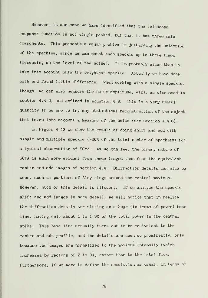
However, in our case we have identified that the telescope
response function is not single peaked, but that it has three main
components. This presents a major problem in justifying the selection
of the speckles, since we can count each speckle up to three times
(depending on the level of the noise). It is probably wiser then to
take into account only the brightest speckle. Actually we have done
both and found little difference. When working with a single speckle,
though, we can also measure the noise amplitude, <r(x), as discussed in
section 4.4.3, and defined in equation 4.9. This is a very useful
quantity if we are to try any statistical reconstruction of the object
that takes into account a measure of the noise (see section 4.4.6).
In Figure 4. 12 we show the result of doing shift and add with
single and multiple speckle (-207. of the total number of speckles) for
a typical observation of SCrA. As we can see, the binary nature of
SCrA is much more evident from these images than from the equivalent
center and add images of section 4.4. Diffraction details C8in also be
seen, such as portions of Airy rings around the central maximum.
However, much of this detail is illusory. If we analyze the speckle
shift said add images in more detail, we will notice that in reality
the diffraction details are sitting on a huge (in terms of power) base
line, having only about 1 to 1.5% of the total power in the central
spike. This base line actually turns out to be equivalent to the
center and add profile, and the details are seen so prominently, only
because the images are normalized to the maximum intensity (which
increases by factors of 2 to 3), rather than to the total flux.
Furthermore, if we were to define the resolution as usual, in terms of
76
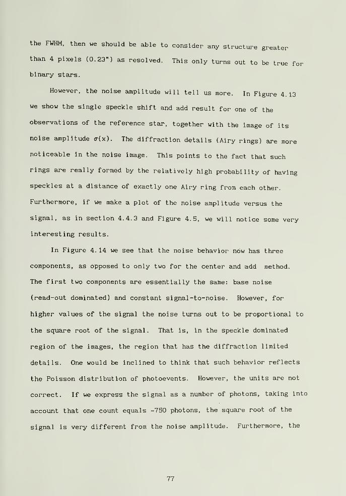
the FWHM, then we should be able to consider any structure great(
than 4 pixels (0.23") as resolved. This only turns out to be true for
binai'y stars.
However, the noise amplitude will tell us more. In Figure 4.13
we show the single speckle shift and add result for one of the
observations of the reference star, together with the image of its
noise amplitude (r(x). The diffraction details (Airy rings) are more
noticeable in the noise image. This points to the fact that such
rings are really formed by the relatively high probability of having
speckles at a distance of exactly one Airy ring from each other.
Furthermore, if we make a plot of the noise amplitude versus the
signal, as in section 4.4.3 and Figure 4.5, we will notice some very
interesting results.
In Figure 4. 14 we see that the noise behavior now has three
components, as opposed to only two for the center and add method.
The first two components are essentially the same: base noise
(read-out dominated) and constant signal-to-noise. However, for
higher values of the signal the noise turns out to be proportional to
the square root of the signal. That is, in the speckle dominated
region of the images, the region that has the diffraction limited
details. One would be inclined to think that such behavior reflects
the Poisson distribution of photoevents. However, the units are not
correct. If we express the signal as a number of photons, taJcing into
account that one count equals -750 photons, the square root of the
signal is very different from the noise amplitude. Furthermore, the
77
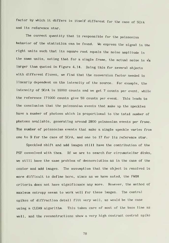
factor by which it differs is itself different for the case of SCrA
and its reference star.
The correct quantity that is responsible for the poissonian
behavior of the statistics can be found. We express the signal in the
right units such that its square root equals the noise amplitude in
the same units, noting that for a single frame, the actual noise is v'm
larger than quoted in Figure 4.14. Doing this for several objects
with different fluxes, we find that the conversion factor needed is
linearly dependent on the intensity of the source. For example, the
intensity of SCrA is 19000 counts and we get 7 counts per event, while
the reference 171000 counts give 59 counts per event. This leads to
the conclusion that the poissonian events that make up the speckles
have a number of photons which is proportional to the total number of
photons available, generating around 2800 poissonian events per frame.
The number of poissonian events that make a single speckle varies from
one to 9 for the case of SCrA, and one to 17 for its reference star.
Speckled shift and add images still have the contribution of the
PSF convolved with them. If we are to search for circumstel lar disks,
we still have the same problem of deconvolution as in the case of the
center and add images. The assumption that the object is resolved is
more difficult to define here, since as we have noted, the FWHM
criteria does not have significance any more. However, the method of
maximum entropy seems to work well for these images. The central
spikes of diffraction detail fitt very well, as would be the case
using a CLEAN algorithm. This takes care of most of the base line as
well, and the reconstructions show a very high contrast central spike
78
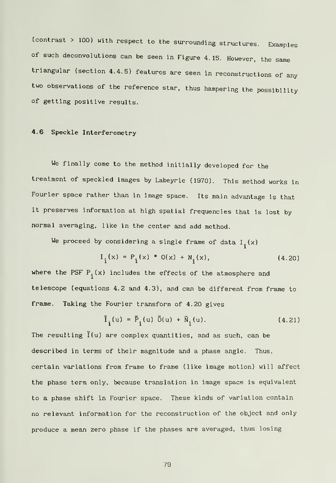
(contrast > 100) with respect to the surrounding structures. Examples
of such deconvolutions can be seen in Figure 4.15. However, the same
triangular (section 4.4.5) features are seen in reconstructions of any
two observations of the reference star, thus hampering the possibility
of getting positive results.
4.6 Speckle Interferoroetry
We finally come to the method initially developed for the
treatment of speckled images by Labeyrie (1970). This method works in
Fourier space rather than in image space. Its main advantage is that
it preserves information at high spatial frequencies that is lost by
normal averaging, like in the center and add method.
We proceed by considering a single frame of data I^(x)
I.(x) = P^(x) * 0(x) + N.(x), (4.20)
where the PSF P^(x) includes the effects of the atmosphere and
telescope (equations 4.2 and 4.3). and can be different from frajne to
frajne. Taking the Fourier transform of 4.20 gives
I.(u) = P.(u) 0(u) + N.(u). (4.21)
The resulting I(u) are complex quantities, and as such, can be
described in terms of their magnitude and a phase angle. Thus,
certain variations from frame to frame (like image motion) will affect
the phase term only, because translation in image space is equivalent
to a phase shift in Fourier space. These kinds of variation contain
no relevant information for the reconstruction of the object and only
produce a mean zero phase if the phases are averaged, thus losing
79
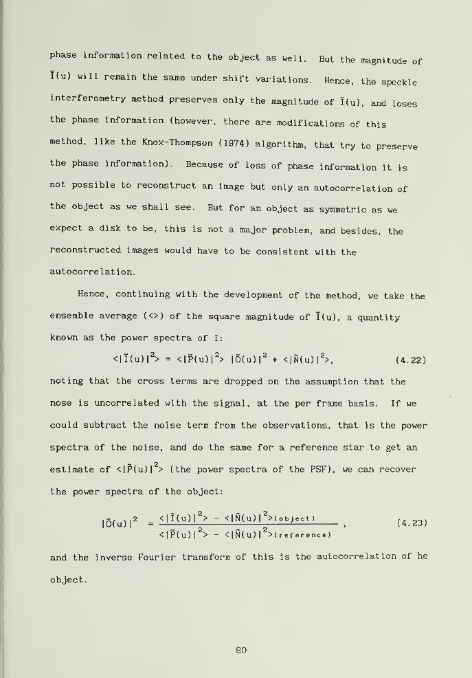
phase information related to the object as well. But the magnitude of
I(u) will remain the same under shift variations. Hence, the speckle
interferometry method preserves only the magnitude of I(u). and loses
the phase information (however, there are modifications of this
method, like the Knox-Thompson (1974) algorithm, that try to preserve
the phase information). Because of loss of phase information it is
not possible to reconstruct an image but only an autocorrelation of
the object as we shall see. But for an object as symmetric as we
expect a disk to be, this is not a major problem, and besides, the
reconstructed images would have to be consistent with the
autocorrelation.
Hence, continuing with the development of the method, we take the
ensemble average (<>) of the square magnitude of T(u). a quantity
known as the power spectra of I:
<|I(u)|S = <|P(u)|S |0(u)|^ + <|N(u)|S, (4.22)
noting that the cross terms su^e dropped on the assumption that the
nose is uncorrelated with the signal, at the per frame basis. If we
could subtract the noise term from the observations, that is the power
spectra of the noise, and do the same for a reference star to get an
estimate of <|P(u)| > (the power spectra of the PSF), we can recover
the power spectra of the object:
|6(u)2 ^ <|I(u)|^> - <|N(U) I^XobJect)
<|P(u)|^> - < |N(u) I reference)
and the inverse Fourier transform of this is the autocorrelation of he
object.
80
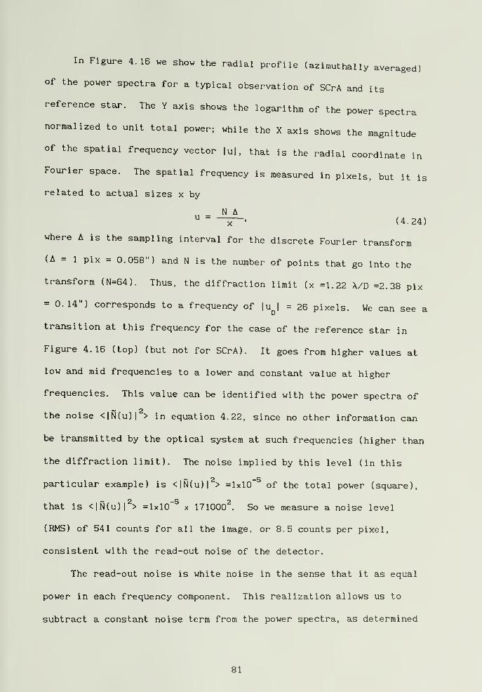
In Figure 4.16 we show the radial profile (azimuthally averaged)
of the power spectra for a typical observation of SCrA and its
reference star. The Y axis shows the logarithm of the power spectra
normalized to unit total power; while the X axis shows the magnitude
of the spatial frequency vector |u|. that is the radial coordinate in
Fourier space. The spatial frequency is measured in pixels, but it is
related to actual sizes x by
_ N A^ (4.24)
where A is the sampling interval for the discrete Fourier transform
(A = 1 pix = 0.058") and N is the number of points that go into the
transform (N=64). Thus, the diffraction limit (x =1.22 A/D =2.38 pix
= 0.14") corresponds to a frequency of |u^| = 26 pixels. We can see a
transition at this frequency for the case of the reference star in
Figure 4.16 (top) (but not for SCrA). It goes from higher values at
low and mid frequencies to a lower and constajit value at higher
frequencies. This value can be identified with the power spectra of
the noise <|N(u)| > in equation 4.22, since no other information can
be transmitted by the optical system at such frequencies (higher than
the diffraction limit). The noise implied by this level (in this
particular example) is <|N(u)|^> =1x10"^ of the total power (square),
that is <|N(u)|S =lxlO~^ x 171000^. So we measure a noise level
(RMS) of 541 counts for all the image, or 8.5 counts per pixel,
consistent with the read-out noise of the detector.
The read-out noise is white noise in the sense that it as equal
power in each frequency component. This realization allows us to
subtract a constant noise term from the power spectra, as determined
81
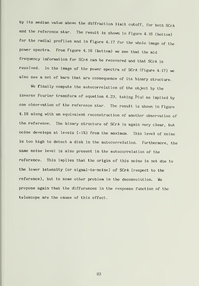
by its median value above the diffraction limit cutoff, for both SCrA
and the reference star. The result is shown in Figure 4.16 (bottom)
for the radial profiles and in Figure 4.17 for the whole image of the
power spectra. From Figure 4.16 (bottom) we see that the mid
frequency information for SCrA can be recovered and that SCrA is
resolved. In the image of the power spectra of SCrA (Figure 4.17) we
also see a set of bars that are consequence of its binary structure.
We finally compute the autocorrelation of the object by the
inverse Fourier transform of equation 4.23, taking P(u) as implied by
one observation of the reference star. The result is shown in Figure
4.18 along with an equivalent reconstruction of another observation of
the reference. The binary structure of SCrA is again very clear, but
noise develops at levels (-1%) from the maximum. This level of noise
is too high to detect a disk in the autocorrelation. Furthermore, the
same noise level is also present in the autocorrelation of the
reference. This implies that the origin of this noise is not due to
the lower intensity (or signal-to-noise) of SCrA (respect to the
reference), but to some other problem in the deconvolution. We
propose again that the differences in the response function of the
telescope are the cause of this effect.
82
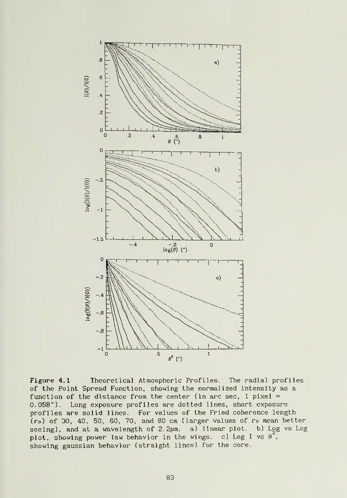
Figure 4.1 Theoretical Atmospheric Profiles. The radial profilesof the Point Spread Function, showing the normalized intensity as a
function of the distance from the center (in arc sec, 1 pixel =
0.058"). Long exposure profiles are dotted lines, short exposure
profiles are solid lines. For values of the Fried coherence length
(ro) of 30, 40, 50, 60, 70, and 80 cm (larger values of ro mean better
seeing), and at a wavelength of 2.2fim. a) linear plot, b) Log vs Log
plot, showing power law behavior in the wings, c) Log I vs 9 ,
showing gaussian behavior (straight lines) for the core.
83
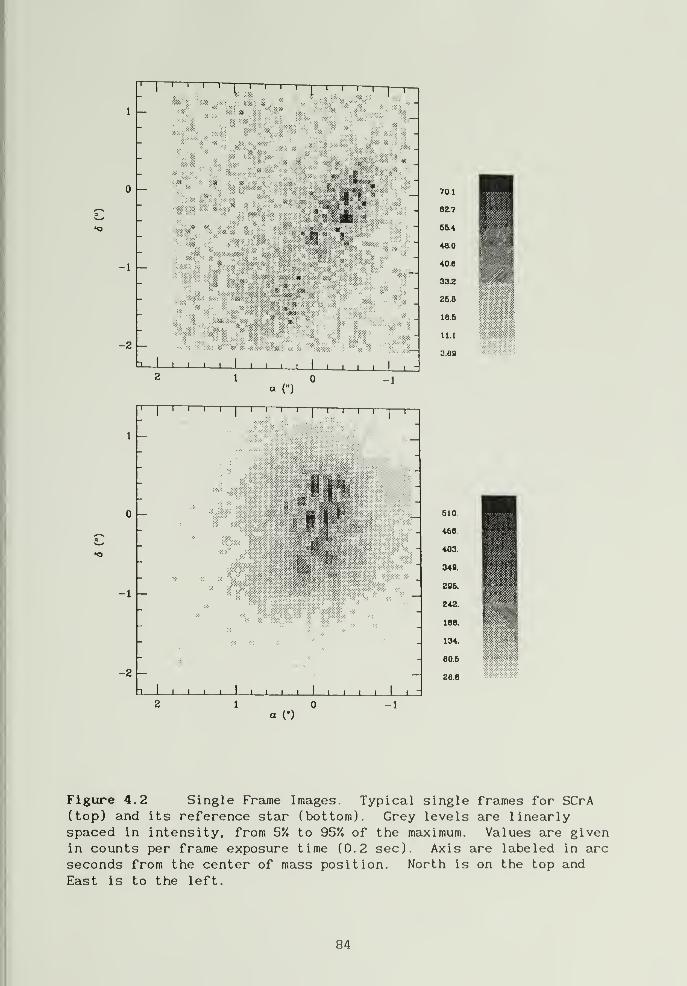
Figure 4.2 Single Frame Images. Typical single frames for SCrA(top) and its reference star (bottom). Grey levels are linearlyspaced in intensity, from 5% to 95% of the maximum. Values are givenin counts per frame exposure time (0.2 sec). Axis are labeled in arcseconds from the center of mass position. North is on the top and
East is to the left.
84
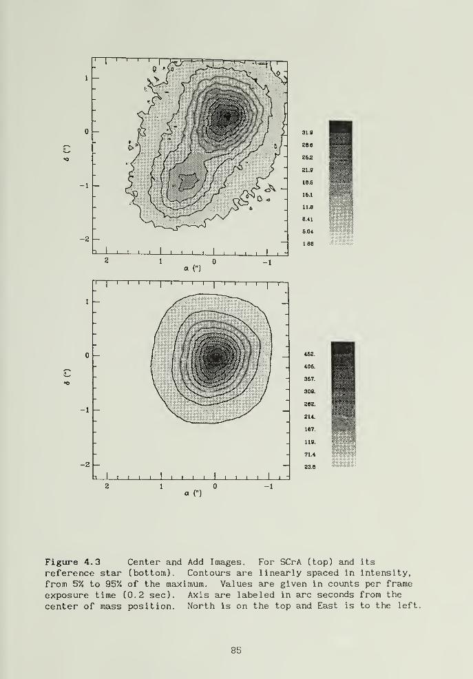
3—I I I I 1 I 1 I I I I I I I I I i_;
2 10-1a (")
Figure 4.3 Center and Add Images. For SCrA (top) ajid its
reference staj" (bottom). Contours are linearly spaced in intensity,
from 5% to 95% of the maximum. Values are given in counts per frame
exposure time (0.2 sec). Axis are labeled in arc seconds from the
center of mass position. North is on the top and East is to the left.
85
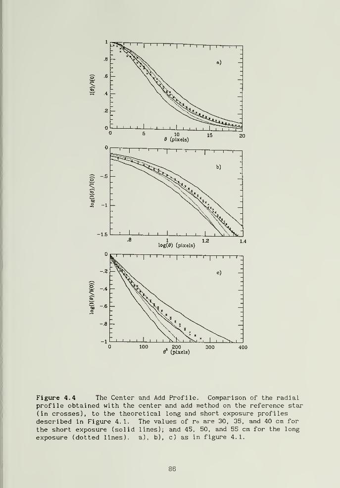
Figure 4.4 The Center and Add Profile. Comparison of the radialprofile obtained with the center and add method on the reference star
(in crosses), to the theoretical long and short exposure profiles
described in Figure 4.1. The values of ro are 30, 35, and 40 cm for
the short exposure (solid lines); and 45, 50, and 55 cm for the long
exposure (dotted lines). a), b), c) as in figure 4.1.
86
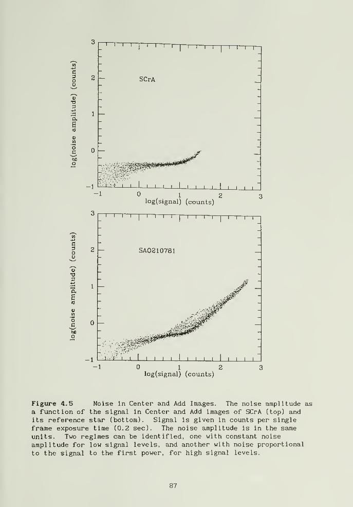
-1 0,1 2log(signal) (counts)
1—I
—
\—
r
n—
r
"I—
r
SA02 10781
•a3
0)
v>
o
o
-1 J ^ \ L
-1 0 1 2log(signal) (counts)
J I L
Figure 4.5 Noise in Center and Add Images. The noise amplitude as
a function of the signal in Center and Add images of SCrA (top) andits reference star (bottom). Signal is given in counts per single
frame exposure time (0.2 sec). The noise amplitude is in the same
units. Two regimes can be identified, one with constaint noise
amplitude for low signal levels, and another with noise proportional
to the signal to the first power, for high signal levels.
87
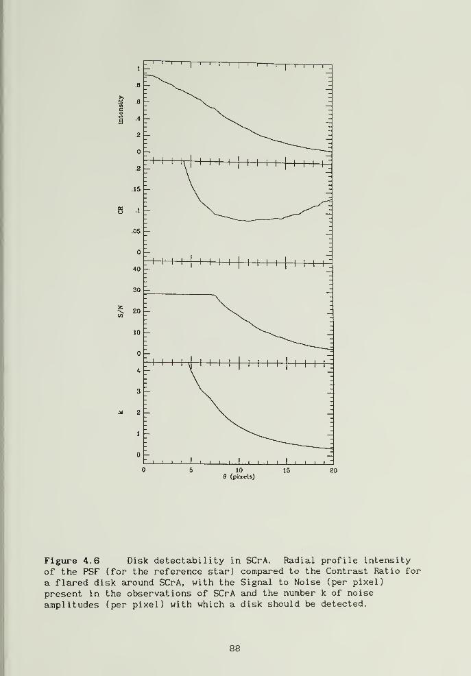
0 - -1-1 1 1 1 1 1 1 I I I I I I
r I I I I I
~
0 5 10 15 200 (pixels)
Figure 4.6 Disk detectabi 1 ity in SCrA. Radial profile intensity
of the PSF (for the reference star) compared to the Contrast Ratio for
a flared disk around SCrA, with the Signal to Noise (per pixel)
present in the observations of SCrA and the number k of noise
amplitudes (per pixel) with which a disk should be detected.
88
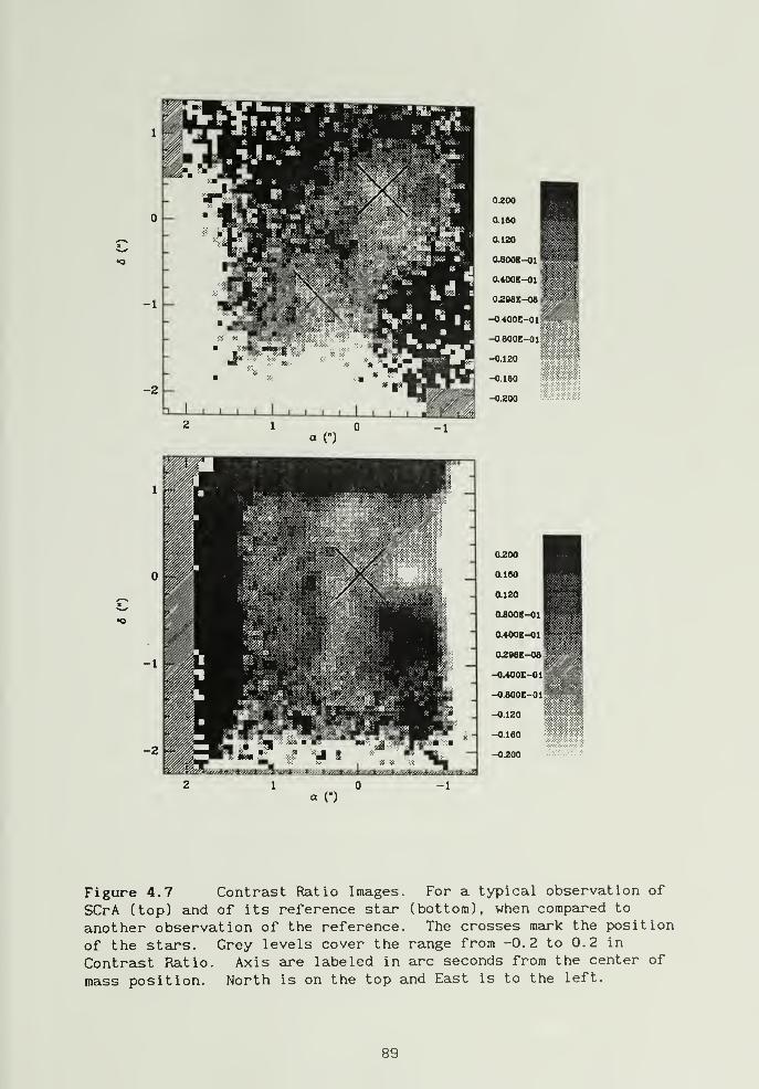
Figure 4.7 Contrast Ratio Images
SCrA (top) and of its reference star
another observation of the reference
of the stars. Grey levels cover the
Contrast Ratio. Axis are labeled in
mass position. North is on the top
For a typical observation of(bottom), when compared to
The crosses mark the positionrange from -0.2 to 0.2 in
arc seconds from the center of
and East is to the left.
89
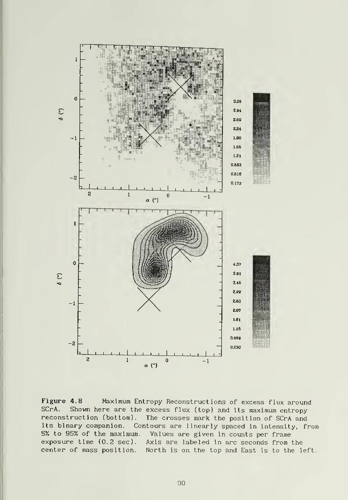
Figure 4,8 Maximum Entropy Reconstructions of excess flux aroundSCrA. Shown here are the excess flux (top) and its maximum entropyreconstruction (bottom). The crosses mark the position of SCrA andits binary companion. Contours are linearly spaced in intensity, from5% to 95% of the maximum. Values are given in counts per frameexposure time (0.2 sec). Axis are labeled in arc seconds from thecenter of mass position. North is on the top and East is to the left.
90

J L J L J L
a (")
-1
Figure 4.9 Telescope response in two different observations. Fortwo observations of the reference star 20 minutes apairt. Contours arelogarithmically spaced from 907. of the maximum at intervals of 0.15dex. Axis are labeled in arc seconds. North is on the top and Eastto the left.
91
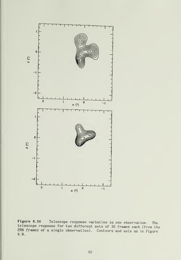
Figure 4,10 Telescope response variation in one observation. Thetelescope response for two different sets of 32 frames each (from the256 frames of a single observation). Contours and axis as in Figure4.8.
92
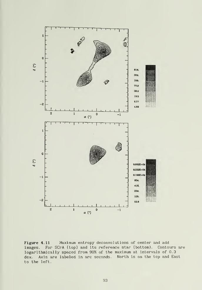
Figure 4.11 Maximum entropy deconvolut ions of center and add
images. For SCrA (top) and its reference star (bottom). Contours are
logarithmically spaced from 90% of the maximum at intervals of 0.3
dex. Axis are labeled in arc seconds. North is on the top and East
to the left.
93
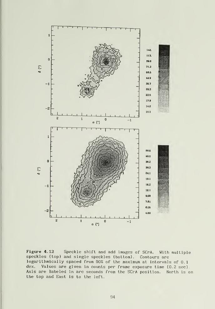
1
Figure 4.12 Speckle shift and add images of SCrA. With multiplespeckles (top) and single speckles (bottom). Contours arelogarithmically spaced from 907. of the maximum at intervals of 0.1dex. Values are given in counts per frame exposure time (0.2 sec).Axis are labeled in arc seconds from the SCrA position. North is onthe top and East is to the left.
94
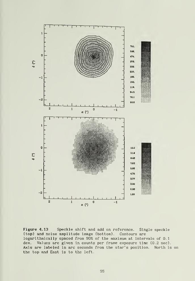
Figure 4.13 Speckle shift and add on reference. Single speckle(top) and noise ajnplitude image (bottom). Contours arelogarithmically spaced from 90% of the meiximum at intervals of 0.1dex. Values are given in counts per frame exposure time (0.2 sec).
Axis are labeled in arc seconds from the star's position. North is on
the top and East is to the left.
95

:3
a,
S(0
o
O
E
I/)
"o
O
0 —
-1
I I I I
I
-T—r—r
SCrA
I I I
I
I I I-
-1
.11 1
-11
1 1 1 1 ' 1 ' 1 1 1 1 10,1 2log(signal) (counts)
1 1 1
a
1 1 11
11 1 1 1
11 1 1 r
I
1
SA02 10781
1 1 1
' '.•
".'' y *.
1 1 1 1 1 1 1 1 1 1 1 1 11 1 1
-1 0 1 2log(signal) (counts)
Figure 4.14 Noise in Speckle Shift and Add Images. The noiseamplitude as a function of the signal in single speckle shift and addimages of SCrA (top) and its reference star (bottom). Signal is givenin counts per single frame exposure time (0.2 sec). The noiseamplitude is in the same units. As in figure 4.5, but a new regimenoise « i/signal is seen for high signal values.
96
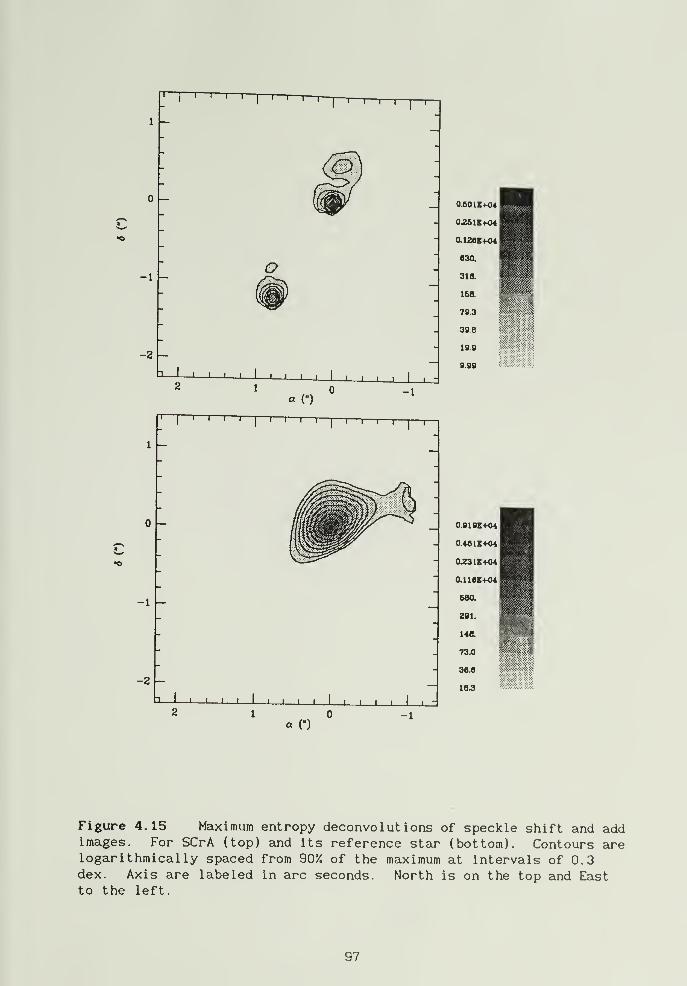
Figure 4.15 Maximum entropy deconvolutions of speckle shift and addimages. For SCrA (top) aind its reference star (bottom). Contours arelogarithmically spaced from 907. of the maximum at intervals of 0.3dex. Axis are labeled in arc seconds. North is on the top and Eastto the left.
97
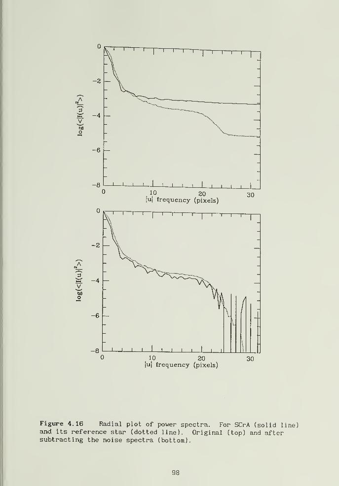
Figure 4.16 Radial plot of power spectra. For SCrA (solid line)and its reference star (dotted line). Original (top) and aftersubtracting the noise spectra (bottom).
98
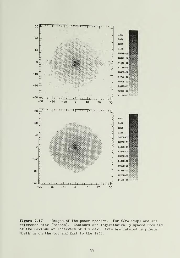
30
20
10
1' ' ' 'I
' ^ ' '
I' ^ ^ ' ' * '
IM I I
I
I I I I
Ij
-10
-20
r^-i I I I I I I I I I I I I I I ' ' ' '1 r I I I I , ,
, I
U
30
-30 -20 -10 0 10 20 30
L' ' ' '
I
I'
I I
I
' ' ' '
I
'' ' '
I
I ' I I
II ' I I
j_
20
10
-10
-20
~30 rf-i I I I I I I I I I I I I I I I I I I I I I r I I I I I . t-
-30 -20 -10 10 20 30
Figure 4.17 Images of the power spectra. For SCrA (top) and itsreference star (bottom). Contours are logarithmically spaced from 90%of the maximum at intervals of 0.3 dex. Axis are labeled in pixels.
North is on the top and East to the left.
99
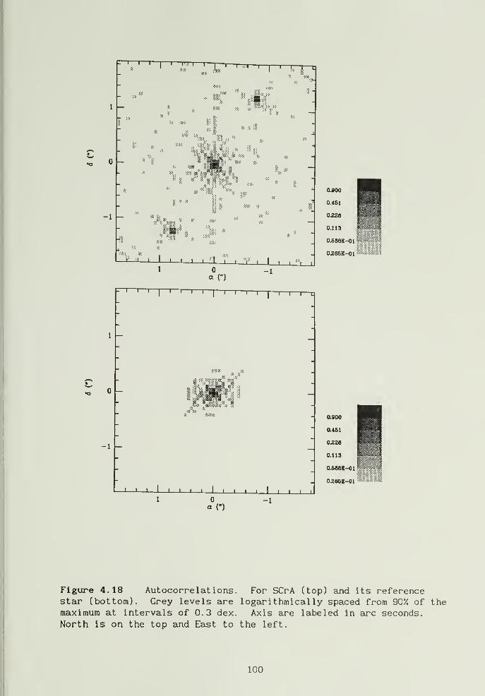
-1
- I 1 1
1
' ^ ' ' J7"T—nn—1—^—
1
!:•
—
§-
-
-
-
...?
'\ ^1^^^^^
- *^ www g jj£.... ..
—-
-
... .,
®
. is*:
-iff
m'i .J 1 1 1 -1—1—i_;t r 1 -i' ,
1 1 1 "l i
0a (")
-1
-1
=~i I II
I—I—I—
r
I
'I
'
'—I—r—I—I—
-J 1 1 1 1 1 1 1 1 I I I I I I t I I
1 0 -1a (")
Figure 4.18 Autocorrelations. For SCrA (top) and its referencestar (bottom). Grey levels are logarithmically spaced from 90% of themaximum at intervals of 0.3 dex. Axis are labeled in arc seconds.
North is on the top and East to the left.
100

CHAPTER 5
SUMMARY OF RESULTS
5.1 Introduction
In this final section, we will briefly address a quantitative
comparison of the different methods used in chapter 4 to study SCrA in
the infrared (chapter 5.2). We will provide with the limiting 3a-
surface brightness that can be recovered with these methods in view of
the unstable telescope response that was observed. Then we will
report the results of the analysis of visible wavelength observations
of SCrA (chapter 5.3). Finally, we will report on the rest of the
infrared survey that we carried out at KPNO (chapter 5.4).
5.2 Observations of SCrA at Infrared Wavelength
In chapter 4 we saw three ways of combining the individual frames
of the observations to produce an image or autocorrelation. These
were a) Center and Add (CA), b) Speckle Shift and Add (SSA), and c)
Speckle Interferometry (SI). A comparison between these follows.
We noted earlier that the SSA and CA methods were essentially
equivalent in that the diffraction limited details seen in the SSA
contained only 1% of the total power and sat on a huge baseline that
resembles the CA. This can be seen in fact by subtracting the CA from
the SSA images as in Figure 5.1, where we show the radial profile of
the difference for SCrA and its reference star. Only diffraction
101
details, as Airy rings persist. In addition, maximum entropy
reconstructions of images obtained with these two methods show
triangular structures. These structures were identified with the lack
of stability of the telescope response function. This is so because
the statistic criteria / is dominated by trying to fit the
differences in PSF's (that amount to //N . 4-5) rather than the
differences between a star alone and a star with a disk [x^/n -1.5).
The surrounding low intensity structure reconstructed with maximum
entropy methods on these images is usually dominated by triangular
structures. This is true even for the SSA images where diffraction
details help the maximum entropy method to find the position of the
star and make it more centrally peaked.
In table 5.1 we give a quantitative comparison of the sensibility
of these methods. There we list the surface brightness that could be
observed at a distance of 0.5" from the star (seeing = 0.9"). with the
maximum entropy method on CA and SSA images (ME CA and ME SSA),
compared to the same results for the contrast ratio method used on CA
images (chapter 4.4.4). and the SI method that will be further
discussed below. The first column in the table tells the method used;
the second column, the surface brightness at which we observe
fictitious structure reconstructed in an observation of an unresolved
star compared to another observation of the same star. As we
concluded in chapter 4.4.5, the variations in the telescope response
can still generate 10'/. variations in the total profile at 0.5" from
the center, so a 2<r detection would be for structures 0.28
2magnitudes/" brighter than the observed values of column 2. So. in
102
:ure
column 3 we list the limiting surface brightness that a struct,
Should have to be a 3. detection, in view of the possible variationsOf the telescope response. Finally, in column 4. we list the observedsurface brightness for structures seen around the star SCrA at 0.5"
(r=75 AU) With each of these methods. For comparison we recall from
chapter 2.4.4. that the surface brightness of a flared disk of q=0.025
is 3.75 mag/"2 fainter than the star at a distance of 0.5".
We can note from table 5.1 that: 1) all the observed structures
around SCrA are fainter than the 3cr limit for detection, so they are
all probably due to differences in the PSF's; 2) that the methods in
image space seem to perform slightly better than the one in Fourier
space (see below); and 3) that the limiting magnitude for a structure
that can be recovered at 0.5" from the star is around 2 mag/"^ which
is brighter than the predicted 3.75 mag/"^ for a flared disk.
A comparison of the results of the SI to the other two methods is
complicated by the difficulty in translating the effects of the
differences in the PSF's to Fourier space. In equation 4.23, the
power spectrum of one observation of a PSF was deconvolved directly
from that of the data. But differences to the actual PSF convolved
with the data will produce false power spectra information for the
object. This additional information is likely to result in the noise
that develops at low intensity levels (-1% of the maximum) in the
autocorrelations, thus hampering the recovery of disk structures. We
can show that this noise level masks the detection of any extended
structure with a surface brightness of more than 1.95 mag/"^ (listed
in table 5.1) fainter than the star, as follows:
103
The central spot in the autocorrelation has a triangular radial
profile with a base of 4.23 pixels. This can consistently arise from
a diffraction limited box of area w (=4.23^) and height H. We take
this as a model for the central star and consider that in the image of
the object 0(x) there is extended emission present at some position x
as well, with height S and extended over an area Q. In this simple
case, the autocorrelation A(x) =J
0(x' ) O(x'-x) dx' . can be written
as A(x) = w-S-H, while at the origin (x=0) A(0) = w(H^S^). We solve
for the value of the intensity S referred to the intensity H and get
A(0) - |^A(0)-4A(x)^JI
/ 2A(x). in terms of the measured value
of the autocorrelation at the point of interest and at the origin.
Furthermore, we are actually interested in the ratio of fluxes from
one square arc second of extended emission to the total flux from the
star which is S-n / H-w for 0=1"^, so we multiply the S/H result
above, by n/w = 1/(0.058x4.23)^ =16.6. A 1% level in the
autocorrelation then corresponds to A(x) = 0.01 (A(0) = 1), so that
S-n/ H-w = 0.166 gives the 1.95 mag/"^ limit referred above and in
table 5. 1.
5.3 Observations of SCrA at Visible Wavelengths
One of the reasons that SCrA is a good candidate for a case study
is that it had been observed in visible wavelengths by Dr. Peter
Nisenson (at the Center for Astrophysics), and we could therefore
compare our results and methods with his. His observations were
104
carried out at CTIO in Chile, using a photon counter camera (the PAPA,
see Nisenson. 1988). with which he obtained several images in the V
filter and in the Hydrogen Ha line filter. His analysis method is of
the SI type, complemented by image reconstructions using an enhanced
Knox-Thompson algorithm.
Dr. Nisenson kindly allowed us to test some of our methods on his
data. It is not possible to apply the SSA method because: a) the
correlation time for atmospheric variations in visible wavelengths is
smaller (~10ms) than in the infrared, and b) the number of speckles is
larger (Ns~300 ). These two factors combine to produce a very small
number of photons per speckle, in fact less than one for the case of
SCrA and most T-Tauri stars, and thus it is not possible to identify
speckle locations.
Therefore, we analyzed his data using the CA images, and
deconvolved the PSF with the maximum entropy technique described in
chapter 4. The noise amplitude suggested from the data has only one
component which is consistent with photon noise. The results are
quite consistent with those obtained by Nisenson doing Knox Thompson
image reconstructions. In summary these results aj-e: a) No evidence
is seen for a flared disk, although we didn't have enough data to see
if the reason may lie in instabilities in the PSF as was the case for
our infrared observations, b) The Ha images were particuleirly
interesting in that they show three components instead of two. That
is, the binary companion to SCrA is not seen in Ha, but instead two
components of emission are seen at different positions in these
images, the brighter one at 0.2" SE of the visible star, and the
105
fainter 0.3" NW of that star. The maximun> entropy reconstruction of
the Ha images is seen in Figure 5.2. where we show the position of the
two stars in the V fields superimposed. These three components are
also seen by Nisenson. In addition he detects a lower intensity
fourth component to the North of the main star, not seen by us. The
analysis of these images is still under way by Nisenson. with a final
interpretation awaiting his results. Nevertheless we can state that
the maximum entropy reconstruction of CA images can give similar
results to SI based methods.
5.4 Rest of Survey
The main results of the rest of the infrared survey that we
carried out at KPNO are described below. As in the case described for
SCrA (chapter 4) the differences in telescope response functions were
predominant. The PSF can be much worse than the one described for
SCrA, but it is never better. As a result of this, a) it was not
possible to recover any low intensity extended structure in our
survey, and b) none of the objects could be identified as extended in
high luminosity (allowing for 30% variations in the intensity
profiles) except for the case of DG-Tau, which seemed to have 40%
excess emission in the EW direction, while less than 5% in the NS
direction.
However, two binary stars were discovered. The first was the
star MWC863, an object that had been classified as enigmatic by Elias
(1978) (object 49 of his survey) because it had silicate emission at
106
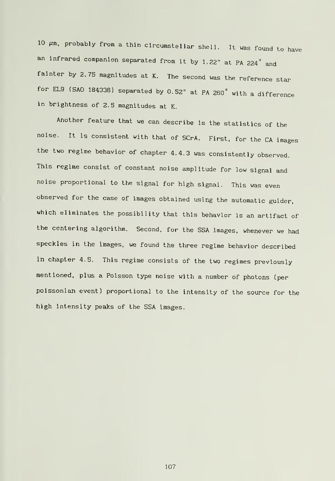
10 Mm. probably from a thin circumstellar shell. It was found to have
an infrared companion separated from it by 1.22" at PA 224° and
fainter by 2.75 magnitudes at K. The second was the reference star
for EL9 (SAO 184336) separated by 0.52" at PA 260° with a difference
in brightness of 2.5 magnitudes at K.
Another feature that we can describe is the statistics of the
noise. It is consistent with that of SCrA. First, for the CA images
the two regime behavior of chapter 4.4.3 was consistently observed.
This regime consist of constant noise amplitude for low signal and
noise proportional to the signal for high signal. This was even
observed for the case of images obtained using the automatic guider,
which eliminates the possibility that this behavior is an artifact of
the centering algorithm. Second, for the SSA images, whenever we had
speckles in the images, we found the three regime behavior described
in chapter 4.5. This regime consists of the two regimes previously
mentioned, plus a Poisson type noise with a number of photons (per
poissonian event) proportional to the intensity of the source for the
high intensity peaks of the SSA images.
107
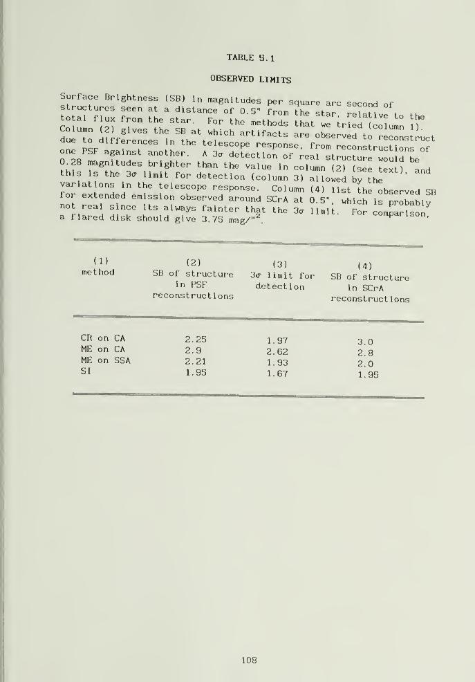
TABLE 5.1
OBSERVED LIMITS
tota, f... rro. the star. ror°ll LiZ: It.T[rT.lTo'll: \Tarto;^.-r„Lr:„^?.:\:?-
r
this s the 30- limit for detection (column 3) allowed by thevarlat ons in the telescope response. Column (4) list the observed SBfor extended emission observed around SCrA at 0.5". which is probablvnot real since its always fainter that the 3<r limi . For compaMsoia flared disk should give 3.75 mag/"^.comparison,
(2) (3) (4)method SB of structure 3o- limit for SB of structure
PSF detection in SCrAreconstructions reconstructions
CR on CAME on CAME on SSASI
2.252.92.21
1.95
1.972.621.93
1.67
3.0
2.8
2.01.95
108
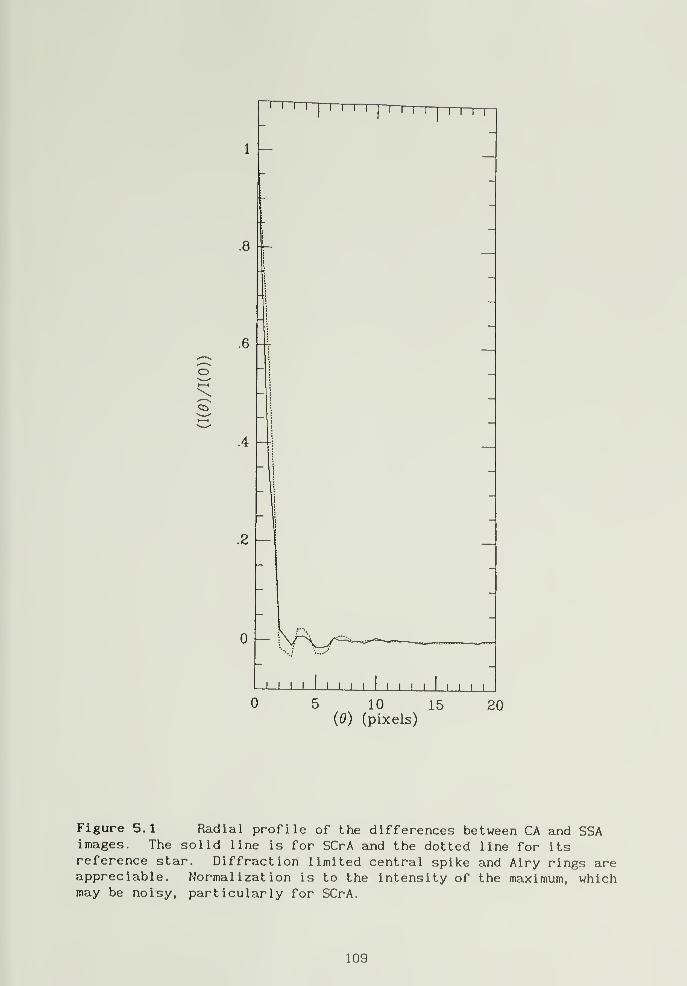
T~r7I I I I I
I
II I I I
I I I I I I I I I I I I I I I I I I
0 5 10 15 20(e) (pixels)
Figure 5.1 Radial profile of the differences between CA and SSAimages. The solid line is for SCrA and the dotted line for itsreference star. Diffraction limited central spike and Airy rings areappreciable. Normalization is to the intensity of the maximum, whichmay be noisy, particularly for SCrA.
109
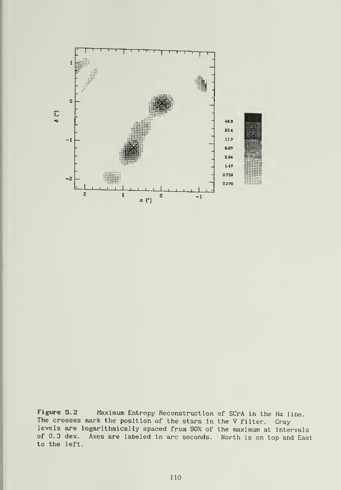
Figure 5.2 Maiximum Entropy Reconstruction of SCrA in the Ha line.The crosses mark the position of the stars in the V filter. Graylevels are logarithmically spaced from 90% of the maximum at intervalsof 0.3 dex. Axes are labeled in arc seconds. North is on top and Eastto the left.
110
CHAPTER 6
CONCLUSION
We have tried to confirm the hypothesis that disks surround young
stars in their formation stage, observing scattered infrared radiation
from dust embedded in such disks, using different super-resolution
techniques. The working hypothesis was that those disks should more
likely be flared, and an experimental verification of that hypothesis
was proposed in terms of a relation between the spectral index and the
flaring constant. The conclusions of this work are three:
1) With the methods used, the existence of flared disks surrounding
young low mass stars in formation could be neither proved nor
disproved, as the unstable response of the telescope limits the
brightness of recoverable extended structures to brighter than
~2 mag/"^ (fainter than the star) at 0.5" from the star, while the
corresponding value for a proposed flared disk was 3.75 mag/"^. which
is well below this limit.
2) The response of the telescope was identified as having three main
components, with typical separations of 0.5 arc sec (and up to one arc
sec) and variations in intensity and position of 307. typically. Such
variations occur in times as short as one minute.
3) The noise behavior in long exposure images in the infrared,
appears to be dominated by noise « signal, possibly due to the low
number of speckles. In addition, the speckle-shift-and-add method
provides the possibility to test the noise behavior statistics of the
speckles themselves. The noise so observed was of the Poisson type.
111
Ics arebut there is evidence that the events that make up that statisti.
not individual photons, but bunches of many, such that the number of
photons in one bunch is proportional to the intensity of the source.
This may prove Labeyrie's (1970) original hypothesis that it is the
tendency of photons to bunch together in each energy state (as a
result of their boson nature) that makes the speckle phenomena.
However, further observations with a variety of integration times,
intensity of the sources and wavelength of observation will be needed
to prove this hypothesis.
Although modern telescopes were designed to provide good spatial
resolutions at the arc second level, we have attempted to obtain
super-resolution up to the sub-arc second level. However, the
response of the instrument has proven to be too unstable to make that
possible. Better stability will probably be achieved with future
telescopes using adaptive optics to overcome not only deformations of
the mirrors, but also to correct for atmospherically induced wave
distortions. Besides, in the near future, the Hubble Space Telescope
will be able to obtain directly high resolution images of stars in
formation, without the problems created by the earth's atmosphere or
gravitational stress.
112
BIBLIOGRAPHY
Adams, F.C., Lada.C.J., Shu.F.H.. 1987, Ap.J., 312. 788.
Adams, F.C., Lada,C.J., Shu,F.H.. 1988, Ap.J., 326. 865.
Ambartsumian.V.A.. 1947. Stellar Evolution and Astrophysiscs. Erevan:
Acad. Sci. Armenian SSR.
Appenzeller.I.. Janckovics, I. . Ostreicher. R. . 1984. Astr.Ap. 141. 108.
Appenzeller, I. . Wolf.B., 1977. Astr.Ap., 54, 713.
Ayers.G.R.. Dainty, J. C, 1988, Opt. Lett., 13, 547.
Beckers, J. M. .Christou, J. C. , Probst,R.G.
, Ridgway, S. T. . Luke,O.V..
1988. in Proceedings of the NOAO-ESO conference on High
Resolution Imaging by Interferometry.
Beckwith.S.,Zuckerman, B. , Strutskie, M. F. , Dyck.H.M.
, 1984, Ap.J., 287,
793.
Beckwith.S. V. W., Sargent , A. I . , Koresco, C. D. , Weintraub. D. , A. , 1989,
Ap.J., 343, 393.
Bertout.C., 1984, Reports on Prgs in Physics, 47, 111.
Born.M., Wolf,E.
, 1959, Principles of Optics, Pergamon Press, NY.
Cabrit.S. , 1987, Private comunicat ion.
Carrasco.L., Strom, S.E., Strom, K.M., 1973, Ap.J., 182, 95.
Castelaz, M. W. , Hackwell , J. A. , Grasdalen, G. L. , Gehrz,R. D. . Gullixon.C.,
1985. Ap.J., 290, 261.
Castelaz, M. W. , Hackwell , J. A. , Grasdalen, G. L. , Gehrz,R.D. , 1986, Ap.J.,
300, 406.
Christou, J. C. , Hege,E.K. , Freeman, J. D. , Ribak,E., 1986, J.O.S.A., A3,
204.
113
Cohen, M.. Kuhi.L.V., 1979, Ap.J. Suppl.
, 41, 733.
Drain, B.T., Lee.H.M., 1984. Ap.J., 285, 89.
Edwards, S. , 1979, PASP, 91, 329.
Edwards, S., Cabrit,S., Strom S E Hevpn T Qfr>^,„ v.ouium.o.c.
, Heyer.i., btrom.K.M., Anderson, E.,
1987. Ap.J.. 321. 473.
Elias.J.H., 1978, Ap.J., 224, 453.
Fried, D.L., 1966, JOSA. 56, 1372.
Grasdalen.G.L.,Strom, K.M., Strom, S.E., 1973, Ap.J., 184, L53.
Grasdalen.G.L.,Strom, S.E., Strom, K.M.. Capps.R.W.
, Thompson. D..
Castelaz,M., 1984, Ap.J., 283. L57.
Greenberg, J.M. 1968 in Stars and Stellar Systems, VII, (University of
Chicago Press), p. 221.
Gull, S. P., Daniel, G. J., 1978, Nature. 272, 686.
Hubble, E. P., 1922, Ap.J., 56, 400.
Jankovics, I. , Appenzel ler, I . , Krautter,J., 1983, PASP, 95, 933.
Jones, B. P., Herbig.G. H. , 1982, AJ, 87. 1223.
Joy.A.H. , 1945, Ap.J., 102. 168.
Kenyon.S.J.. Hartmann.L., 1987, Ap.J., 323, 714.
King, I. R., 1971, PASP, 83, 1971.
Knacke.R.F., Strom, K.M., Strom, S.E.. Young, E.. 1973, Ap.J., 197, 847.
Knox.K.T. , Thompson, B. J. , 1974, Ap.J., 193. L45.
Kolmogorov. A. N. . 1941. Dan. S. S. S. R. , 30 (4). 229.
Korff.D., Dryden.G.. Miller, M.G.. 1972, Opt ics Comm. , 5, 187.
Lada.C.J., Wi Iking, B. A., 1984, Ap.J., 287. 610.
Labeyrie.A. . 1970, Astr.Ap., 6, 85.
Lucy.L.B. , 1974, AJ , 79, 745.
114
Lynden-Bell.D.. Pringle, J. E. , 1974, MNRAS, 168. 603.
Mendoza.V.E.E., 1966. Ap.J., 143. 1010.
Narayan.R..Nityananda. R.
. 1986. Ann. Rev. Astr. Ap. , 24. 127.
Nisenson.P..
1988. Proceedings of the NATO Adv. Stud. Inst, in
Cargese, France.
Pravdo.S.H.. Rodriguez. L. F. . Curiel.S.. Canto. J.. Torrelles. J. M..
Becker. R.H., Sellgren.K.. 1985. Ap.J., 293. L35.
Pringle, J. E. . 1981, Ann. Rev . Astr. Ap., 19. 137.
Roddier.F., 1981, in Progress in Optics, XIX. 281.
Rucinski.S.M., 1985, AJ, 90, 2321.
Rydgen,A.E., Zak,D.S.
, 1987, AJ, 99, 141.
Sargent, A. I. , Beckwith.S., 1987. Ap.J., 323, 294.
Sargent, A. I. , Beckwith,S., Keene,J., Masson,C.
, 1988, Ap.J., 333, 936.
Shakura,N. I. , Sunyaev, R. A. , 1973, Astr.Ap., 24, 337.
Shu,F.H., Adams, F.C., Lizano,S.
, 1987, Ann.Rev.of.Astron.Ap., 25, 23.
Skilling,J., Bryan, R.K., 1984, MNRAS, 211, 111.
Smith, B. A., Terri le, R. J. , 1984, Science 228, 1421.
Stahler,S. W. , 1983, Ap.J., 274. 822.
Strom, K.M., Strom, S.E., Kenyon,S.J., Hartmann,L. , 1988, AJ, 95, 534.
Strom, K.M., Strom, S.E., Edwards, S., Cabrit.S. , Skrutskie, M. F. , 1989,
AJ, 97. 1451. 51.
Strom. S.E., Strom, K.M., Bregman,J., Yost,Y. , 1972. Ap.J., 171. 267.
Strom. S.E.. Strom, K.M., Grasdalen, G. L. , Capps.R. W.. Thompson, D., 1985,
AJ, 90, 12.
Strom, S.E., Strom, K.M., Edwards, S., 1987
NATO, ASI ,Galct. Extrgl .Star. form.
115
Vrba.F.J.. Strom. K.M... Strom. S.E.. Grasdalen. G. L. . 1975. Ap.J., 197.
77.
Vrba.F.J.. Strom. S.E.. Strom. K. M.. 1976. AJ, 81. 958.
Walker. M.F. 1956, Ap.J. Suppl., 23. 365.
Walker, M.F.. 1972, Ap.J., 175. 89.
Wilking.B.A.. Lada.C.J.. 1983. Ap.J., 274. 698.
Wllllngale.R., 1981, MNRAS, 194, 359.
Witt, A. N., 1985, Ap.J., 294, 216.
Young. E.T.. Lada.C.J.. Wilking.B.A., 1986. Ap.J., 304, L45.
116