high speed obstacle avoidance using monocular vision and reinforcement...

High Speed Obstacle Avoidance using Monocular Vision and

Reinforcement Learning

Jeff Michels [email protected] Saxena [email protected] Y. Ng [email protected]

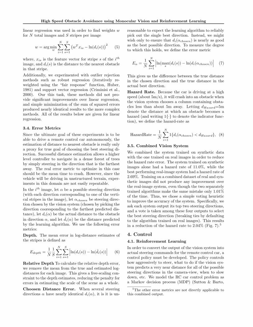
Computer Science Department, Stanford University, Stanford, CA 94305 USA

Abstract

We consider the task of driving a remote con-trol car at high speeds through unstructuredoutdoor environments. We present an ap-proach in which supervised learning is firstused to estimate depths from single monoc-ular images. The learning algorithm can betrained either on real camera images labeledwith ground-truth distances to the closest ob-stacles, or on a training set consisting of syn-thetic graphics images. The resulting algo-rithm is able to learn monocular vision cuesthat accurately estimate the relative depthsof obstacles in a scene. Reinforcement learn-ing/policy search is then applied within asimulator that renders synthetic scenes. Thislearns a control policy that selects a steeringdirection as a function of the vision system’soutput. We present results evaluating thepredictive ability of the algorithm both onheld out test data, and in actual autonomousdriving experiments.

1. Introduction

In this paper, we consider the problem of high speednavigation and obstacle avoidance on a remote controlcar in unstructured outdoor environments. We presenta novel approach to this problem that combines rein-forcement learning (RL), computer graphics, and com-puter vision.

Most work on obstacle detection using vision has fo-cused on binocular vision/steoreopsis. In this paper,we present a monocular vision obstacle detection algo-rithm based on supervised learning. Our motivationfor this is two-fold: First, we believe that single-imagemonocular cues have not been effectively used in most

Appearing in Proceedings of the 22 nd International Confer-ence on Machine Learning, Bonn, Germany, 2005. Copy-right 2005 by the author(s)/owner(s).

obstacle detection systems; thus we consider it an im-portant open problem to develop methods for obstacledetection that exploit these monocular cues. Second,the dynamics and inertia of high speed driving (5m/son a small remote control car) means that obstaclesmust be perceived at a distance if we are to avoid them,and the distance at which standard binocular vision al-gorithms can perceive them is fundamentally limitedby the “baseline” distance between the two camerasand the noise in the observations (Davies, 1997), andthus difficult to apply to our problem.1

To our knowledge, there is little work on depth es-timation from monocular vision in rich, unstructuredenvironments. We propose an algorithm that learnsrelative depth using only monocular visual cues onsingle images of outdoor environments. We collecteda dataset of several thousand images, each correlatedwith a laser range scan that gives the distance to thenearest obstacle in each direction. After training onthis dataset (using the laser range scans as the ground-truth target labels), a supervised learning algorithm isthen able to accurately estimate the distances to thenearest obstacles in the scene. This becomes our basicvision system, the output of which is fed into a higherlevel controller trained using reinforcement learning.

An addition motivation for our work stems fromthe observation that the majority of successfulrobotic applications of RL (including autonomous he-licopter flight, some quadruped/biped walking, snakerobot locomotion, etc.) have relied on model-basedRL (Kearns & Singh, 1999), in which an accuratemodel or simulator of the MDP is first built.2 Incontrol tasks in which the perception problem is non-trivial—such as when the input sensor is a camera—the quality of the simulator we build for the sensor will

1While it is probably possible, given sufficient effort, tobuild a stereo system for this task, the one commercial sys-tem we evaluated (because of vibrations and motion blur)was unable to reliably detect obstacles even at 1m range.

2Some exceptions to this include (Kim & Uther, 2003;Kohl & Stone, 2004).

High Speed Obstacle Avoidance using Monocular Vision and Reinforcement Learning

be limited by the quality of the computer graphics wecan implement. We were interested in asking: Doesmodel-based reinforcement learning still make sense inthese settings?

Since many of the cues that are useful for estimatingdepth can be re-created in synthetic images, we imple-mented a graphical driving simulator. We ran exper-iments in which the real images and laser scan datawas replaced with synthetic images. We also used thegraphical simulator to train a reinforcement learningalgorithm, and ran experiments in which we system-atically varied the level of graphical realism. We showthat, surprisingly, even using low- to medium-qualitysynthetic images, it is often possible to learn depth es-timates that give reasonable results on real camera testimages. We also show that, by combining informationlearned from both the synthetic and the real datasets,the resulting vision system performs better than onetrained on either one of the two. Similarly, the rein-forcement learning controller trained in the graphicalsimulator also performs well in real world autonomousdriving. Videos showing the system’s performance inreal world driving experiments (using the vision sys-tem built with supervised learning, and the controllerlearned using reinforcement learning) are available athttp://ai.stanford.edu/∼asaxena/rccar/

2. Related Work

Broadly, there are three categories of cues that can beused for depth perception from two-dimensional im-ages: monocular cues, stereopsis, and motion parallax(Kudo et al., 1999). By far the most commonly studiedfor this problem is stereo vision (Scharstein & Szeliski,2002). Depth-from-motion or optical flow is based onmotion parallax (Barron et al., 1994). Both methodsrequire finding correspondence between points in mul-tiple images separated over space (stereo) or time (op-tical flow). Assuming that accurate correspondencescan be established, both methods can generate veryaccurate depth estimates. However, the process ofsearching for image correspondences is computation-ally expensive and error prone, which can dramaticallydegrade the algorithm’s overall performance.

A number of researchers have studied how humans usemonocular cues for depth estimation (Loomis, 2001;Wu et al., 2004; Blthoff et al., 1998). Also, (Kardas,2005) presents experiments charaterizing some of thethe different cues’ effects. Such studies done both onhumans and on animals show that cues like texture,texture gradient, linear perspective, occlusion, haze,defocus, and known object size provide information toestimate depth.

Gini (Gini & Marchi, 2002) used single camera vi-

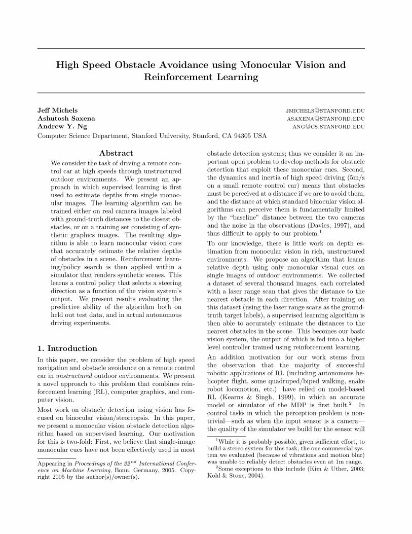
Figure 1. Laser range scans overlaid on the image. Laserscans give one range estimate per degree.

sion to drive a indoor robot, but relied heavily on theknown color and texture of the ground, and hence doesnot generalize well and will fail in unstructured out-door environments. In (Pomerleau, 1989), monocularvision and apprenticeship learning (also called imita-tion learning) was used to drive a car, but only onhighly structured roads and highways with clear lanemarkings, in which the perception problem is mucheasier. (LeCun, 2003) also successfully applied imi-tation learning to driving in richer environments, butrelied on stereo vision. Depth from defocus (Jahne& Geissler, 1994; Honig et al., 1996; Klarquist et al.,1995) is another method to obtain depth estimates,but requires high-quality images, objects with sharpboundaries, and known camera parameters (includingcamera aperture model and modulation transfer func-tion). Nagai (Nagai et al., 2002) built an HMM modelof known face and hand images to recover depth fromsingle images. Shao (Shao et al., 1988) used shapefrom shading to reconstruct depth for objects havingrelatively uniform color and texture.

3. Vision System

We formulate the vision problem as one of depth esti-mation over stripes of the image. The output of thissystem will be fed as input to a higher level controlalgorithm.

In detail, we divide each image into vertical stripes.These stripes can informally be thought of as cor-responding to different steering directions. In orderto learn to estimate distances to obstacles in outdoorscenes, we collected a dataset of several thousand out-door images (Fig. 1). Each image is correlated witha laser range scan (using a SICK laser range finder,along with a mounted webcam of resolution 352x288,Fig. 2), that gives the distance to the nearest obsta-


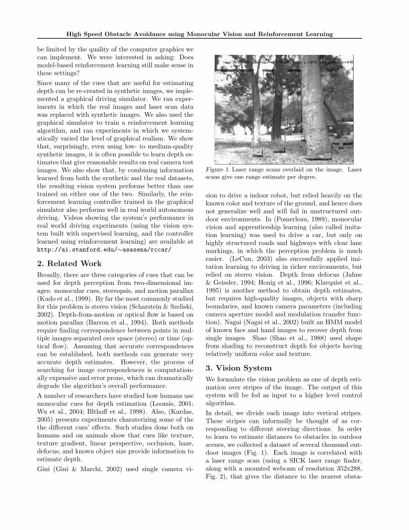
Figure 2. Rig for collecting correlated laser range scans andreal camera images.

cle in each stripe of the image. We create a spatiallyarranged vector of local features capturing monoculardepth cues. To capture more of the global context,the feature vector of each stripe is augmented withthe features of the stripe to the left and right. We uselinear regression on these features to learn to predictthe relative distance to the nearest obstacle in each ofthe vertical stripes.

Since many of the cues that we used to estimate depthcan be re-created in synthetic images, we also devel-oped a custom driving simulator with a variable levelof graphical realism. By repeating the above learningmethod on a second data set consisting of synthetic im-ages, we learn depth estimates from synthetic imagesalone. Additionally, we combine information learnedfrom the synthetic dataset with that learned from realimages, to produce a vision system that performs bet-ter than either does individually.

3.1. Synthetic Graphics Data

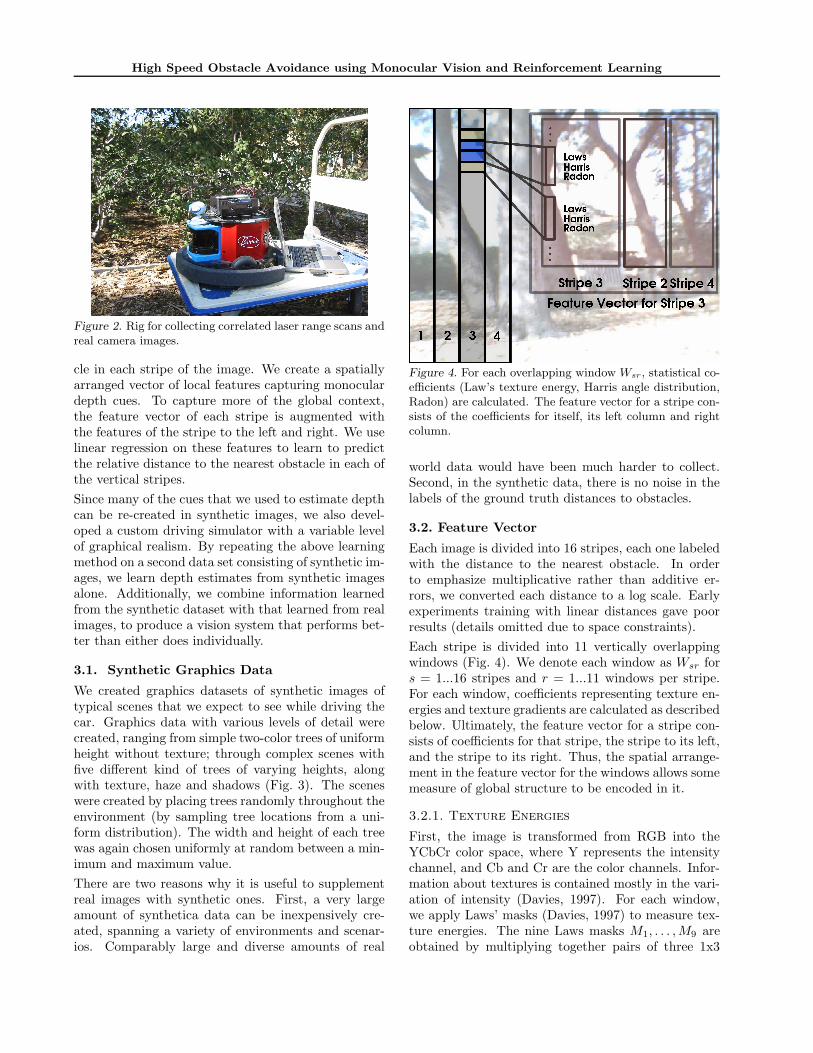
We created graphics datasets of synthetic images oftypical scenes that we expect to see while driving thecar. Graphics data with various levels of detail werecreated, ranging from simple two-color trees of uniformheight without texture; through complex scenes withfive different kind of trees of varying heights, alongwith texture, haze and shadows (Fig. 3). The sceneswere created by placing trees randomly throughout theenvironment (by sampling tree locations from a uni-form distribution). The width and height of each treewas again chosen uniformly at random between a min-imum and maximum value.

There are two reasons why it is useful to supplementreal images with synthetic ones. First, a very largeamount of synthetica data can be inexpensively cre-ated, spanning a variety of environments and scenar-ios. Comparably large and diverse amounts of real

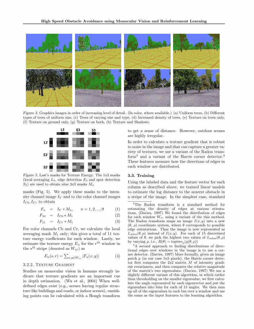
Figure 4. For each overlapping window Wsr, statistical co-efficients (Law’s texture energy, Harris angle distribution,Radon) are calculated. The feature vector for a stripe con-sists of the coefficients for itself, its left column and rightcolumn.

world data would have been much harder to collect.Second, in the synthetic data, there is no noise in thelabels of the ground truth distances to obstacles.

3.2. Feature Vector

Each image is divided into 16 stripes, each one labeledwith the distance to the nearest obstacle. In orderto emphasize multiplicative rather than additive er-rors, we converted each distance to a log scale. Earlyexperiments training with linear distances gave poorresults (details omitted due to space constraints).

Each stripe is divided into 11 vertically overlappingwindows (Fig. 4). We denote each window as Wsr fors = 1...16 stripes and r = 1...11 windows per stripe.For each window, coefficients representing texture en-ergies and texture gradients are calculated as describedbelow. Ultimately, the feature vector for a stripe con-sists of coefficients for that stripe, the stripe to its left,and the stripe to its right. Thus, the spatial arrange-ment in the feature vector for the windows allows somemeasure of global structure to be encoded in it.

3.2.1. Texture Energies

First, the image is transformed from RGB into theYCbCr color space, where Y represents the intensitychannel, and Cb and Cr are the color channels. Infor-mation about textures is contained mostly in the vari-ation of intensity (Davies, 1997). For each window,we apply Laws’ masks (Davies, 1997) to measure tex-ture energies. The nine Laws masks M1, . . . ,M9 areobtained by multiplying together pairs of three 1x3


Figure 3. Graphics images in order of increasing level of detail. (In color, where available.) (a) Uniform trees, (b) Differenttypes of trees of uniform size, (c) Trees of varying size and type, (d) Increased density of trees, (e) Texture on trees only,(f) Texture on ground only, (g) Texture on both, (h) Texture and Shadows.

Figure 5. Law’s masks for Texture Energy. The 1x3 masks(local averaging L3, edge detection E3 and spot detectionS3) are used to obtain nine 3x3 masks Mn

masks (Fig. 5). We apply these masks to the inten-sity channel image IY and to the color channel imagesICb, ICr to obtain

Fn = IY ∗ Mn, n = 1, 2, ..., 9 (1)

F10 = ICb ∗ M1 (2)

F11 = ICr ∗ M1 (3)

For color channels Cb and Cr, we calculate the localaveraging mask M1 only; this gives a total of 11 tex-ture energy coefficients for each window. Lastly, weestimate the texture energy En for the rth window inthe sth stripe (denoted as Wsr) as

En(s, r) =∑

x,y∈Wsr

|Fn(x, y)| (4)

3.2.2. Texture Gradient

Studies on monocular vision in humans strongly in-dicate that texture gradients are an important cuein depth estimation. (Wu et al., 2004) When well-defined edges exist (e.g., scenes having regular struc-ture like buildings and roads, or indoor scenes), vanish-ing points can be calculated with a Hough transform

to get a sense of distance. However, outdoor scenesare highly irregular.

In order to calculate a texture gradient that is robustto noise in the image and that can capture a greater va-riety of textures, we use a variant of the Radon trans-form3 and a variant of the Harris corner detector.4

These features measure how the directions of edges ineach window are distributed.

3.3. Training

Using the labeled data and the feature vector for eachcolumn as described above, we trained linear modelsto estimate the log distance to the nearest obstacle ina stripe of the image. In the simplest case, standard

3The Radon transform is a standard method forestimating the density of edges at various orienta-tions. (Davies, 1997) We found the distribution of edgesfor each window Wsr using a variant of the this method.The Radon transform maps an image I(x, y) into a new(θ, ρ) coordinate system, where θ corresponds to possibleedge orientations. Thus the image is now represented asIradon(θ, ρ) instead of I(x, y). For each of 15 discretizedvalues of θ, we pick the highest two values of Iradon(θ, ρ)by varying ρ, i.e., R(θ) = toptwoρ(g(θ, ρ))

4A second approach to finding distributions of direc-tional edges over windows in the image is to use a cor-ner detector. (Davies, 1997) More formally, given an imagepatch p (in our case 5x5 pixels), the Harris corner detec-tor first computes the 2x2 matrix M of intensity gradi-ent covariances, and then compares the relative magnitudeof the matrix’s two eigenvalues. (Davies, 1997) We use aslightly different variant of this algorithm, in which ratherthan thresholding on the smaller eigenvalue, we first calcu-late the angle represented by each eigenvector and put theeigenvalues into bins for each of 15 angles. We then sumup all of the eigenvalues in each bin over a window and usethe sums as the input features to the learning algorithm.


linear regression was used in order to find weights w

for N total images and S stripes per image

w = arg minw

N∑

i=1

S∑

s=1

(

wT xis − ln(di(s)))2

(5)

where, xis is the feature vector for stripe s of the ith

image, and di(s) is the distance to the nearest obstaclein that stripe.

Additionally, we experimented with outlier rejectionmethods such as robust regression (iteratively re-weighted using the “fair response” function, Huber,1981) and support vector regression (Criminisi et al.,2000). Our this task, these methods did not pro-vide significant improvements over linear regression,and simple minimization of the sum of squared errorsproduced nearly identical results to the more complexmethods. All of the results below are given for linearregression.

3.4. Error Metrics

Since the ultimate goal of these experiments is to beable to drive a remote control car autonomously, theestimation of distance to nearest obstacle is really onlya proxy for true goal of choosing the best steering di-rection. Successful distance estimation allows a higherlevel controller to navigate in a dense forest of treesby simply steering in the direction that is the farthestaway. The real error metric to optimize in this caseshould be the mean time to crash. However, since thevehicle will be driving in unstructured terrain, exper-iments in this domain are not easily repeatable.

In the ith image, let α be a possible steering direction(with each direction corresponding to one of the verti-cal stripes in the image), let αchosen be steering direc-tion chosen by the vision system (chosen by picking thedirection cooresponding to the farthest predicted dis-tance), let di(α) be the actual distance to the obstacle

in direction α, and let d̂i(α) be the distance predictedby the learning algorithm. We use the following errormetrics:

Depth. The mean error in log-distance estimates ofthe stripes is defined as

Edepth =1

N

1

S

N∑

i=1

S∑

s=1

∣

∣

∣ln(di(s)) − ln(d̂i(s))

∣

∣

∣(6)

Relative Depth To calculate the relative depth error,we remove the mean from the true and estimated log-distances for each image. This gives a free-scaling con-straint to the depth estimates, reducing the penalty forerrors in estimating the scale of the scene as a whole.

Choosen Distance Error. When several steeringdirections α have nearly identical di(α), it is it is un-

reasonable to expect the learning algorithm to reliablypick out the single best direction. Instead, we mightwish only to ensure that di(αchosen) is nearly as goodas the best possible direction. To measure the degreeto which this holds, we define the error metric

Eα =1

N

N∑

i=1

∣

∣

∣ln(max

s(di(s)) − ln(di(αchosen))

∣

∣

∣(7)

This gives us the difference between the true distancein the chosen direction and the true distance in theactual best direction.

Hazard Rate. Because the car is driving at a highspeed (about 5m/s), it will crash into an obstacle whenthe vision system chooses a column containing obsta-cles less than about 5m away. Letting dHazard=5mdenote the distance at which an obstacle becomes ahazard (and writing 1{·} to denote the indicator func-tion), we define the hazard-rate as

HazardRate =1

N

N∑

i=1

1{di(αchosen) < dHazard}, (8)

3.5. Combined Vision System

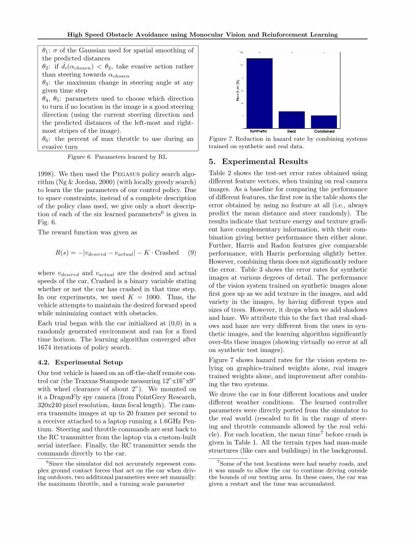
We combined the system trained on synthetic datawith the one trained on real images in order to reducethe hazard rate error. The system trained on syntheticimages alone had a hazard rate of 11.0%, while thebest performing real-image system had a hazard rate of2.69%. Training on a combined dataset of real and syn-thetic images did not produce any improvement overthe real-image system, even though the two separatelytrained algorithms make the same mistake only 1.01%of the time. Thus, we chose a simple voting heuristicto improve the accuracy of the system. Specifically, weask each system output its top two steering directions,and a vote is taken among these four outputs to selectthe best steering direction (breaking ties by defaultingto the algorithm trained on real images). This resultsin a reduction of the hazard rate to 2.04% (Fig. 7).5

4. Control

4.1. Reinforcement Learning

In order to convert the output of the vision system intoactual steering commands for the remote control car, acontrol policy must be developed. The policy controlshow aggressively to steer, what to do if the vision sys-tem predicts a very near distance for all of the possiblesteering directions in the camera-view, when to slowdown, etc. We model the RC car control problem asa Markov decision process (MDP) (Sutton & Barto,

5The other error metrics are not directly applicable tothis combined output.


θ1: σ of the Gaussian used for spatial smoothing ofthe predicted distancesθ2: if d̂i(αchosen) < θ2, take evasive action ratherthan steering towards αchosen

θ3: the maximum change in steering angle at anygiven time stepθ4, θ5: parameters used to choose which directionto turn if no location in the image is a good steeringdirection (using the current steering direction andthe predicted distances of the left-most and right-most stripes of the image).θ6: the percent of max throttle to use during anevasive turn

Figure 6. Parameters learned by RL

1998). We then used the Pegasus policy search algo-rithm (Ng & Jordan, 2000) (with locally greedy search)to learn the the parameters of our control policy. Dueto space constraints, instead of a complete descriptionof the policy class used, we give only a short descrip-tion of each of the six learned parameters6 is given inFig. 6.

The reward function was given as

R(s) = −|vdesired − vactual| − K · Crashed (9)

where vdesired and vactual are the desired and actualspeeds of the car, Crashed is a binary variable statingwhether or not the car has crashed in that time step.In our experiments, we used K = 1000. Thus, thevehicle attempts to maintain the desired forward speedwhile minimizing contact with obstacles.

Each trial began with the car initialized at (0,0) in arandomly generated environment and ran for a fixedtime horizon. The learning algorithm converged after1674 iterations of policy search.

4.2. Experimental Setup

Our test vehicle is based on an off-the-shelf remote con-trol car (the Traxxas Stampede measuring 12”x16”x9”with wheel clearance of about 2”). We mounted onit a DragonFly spy camera (from PointGrey Research,320x240 pixel resolution, 4mm focal length). The cam-era transmits images at up to 20 frames per second toa receiver attached to a laptop running a 1.6GHz Pen-tium. Steering and throttle commands are sent back tothe RC transmitter from the laptop via a custom-builtserial interface. Finally, the RC transmitter sends thecommands directly to the car.

6Since the simulator did not accurately represent com-plex ground contact forces that act on the car when driv-ing outdoors, two additional parameters were set manually:the maximum throttle, and a turning scale parameter

Figure 7. Reduction in hazard rate by combining systemstrained on synthetic and real data.

5. Experimental Results

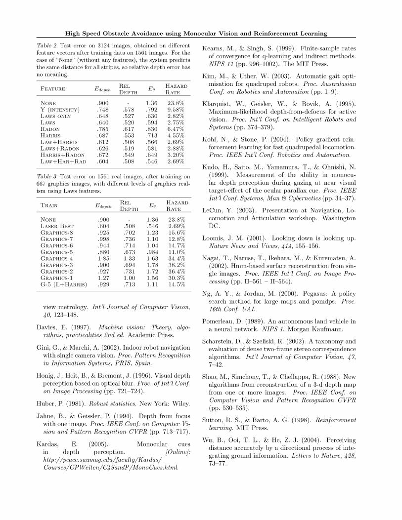
Table 2 shows the test-set error rates obtained usingdifferent feature vectors, when training on real cameraimages. As a baseline for comparing the performanceof different features, the first row in the table shows theerror obtained by using no feature at all (i.e., alwayspredict the mean distance and steer randomly). Theresults indicate that texture energy and texture gradi-ent have complementary information, with their com-bination giving better performance then either alone.Further, Harris and Radon features give comparableperformance, with Harris performing slightly better.However, combining them does not significantly reducethe error. Table 3 shows the error rates for syntheticimages at various degrees of detail. The performanceof the vision system trained on synthetic images alonefirst goes up as we add texture in the images, and addvariety in the images, by having different types andsizes of trees. However, it drops when we add shadowsand haze. We attribute this to the fact that real shad-ows and haze are very different from the ones in syn-thetic images, and the learning algorithm significantlyover-fits these images (showing virtually no error at allon synthetic test images).

Figure 7 shows hazard rates for the vision system re-lying on graphics-trained weights alone, real imagestrained weights alone, and improvement after combin-ing the two systems.

We drove the car in four different locations and underdifferent weather conditions. The learned controllerparameters were directly ported from the simulator tothe real world (rescaled to fit in the range of steer-ing and throttle commands allowed by the real vehi-cle). For each location, the mean time7 before crash isgiven in Table 1. All the terrain types had man-madestructures (like cars and buildings) in the background.

7Some of the test locations were had nearby roads, andit was unsafe to allow the car to continue driving outsidethe bounds of our testing area. In these cases, the car wasgiven a restart and the time was accumulated.


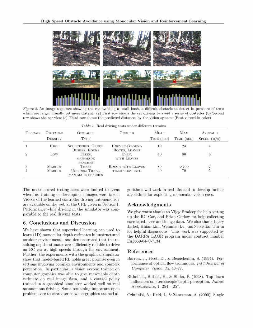
Figure 8. An image sequence showing the car avoiding a small bush, a difficult obstacle to detect in presence of treeswhich are larger visually yet more distant. (a) First row shows the car driving to avoid a series of obstacles (b) Secondrow shows the car view (c) Third row shows the predicted distances by the vision system. (Best viewed in color)

Table 1. Real driving tests under different terrains

Terrain Obstacle Obstacle Ground Mean Max Average

Density Type Time (sec) Time (sec) Speed (m/s)

1 High Sculptures, Trees, Uneven Ground 19 24 4Bushes, Rocks Rocks, Leaves

2 Low Trees, Even, 40 80 6man-made with Leavesbenches

3 Medium Trees Rough with Leaves 80 >200 24 Medium Uniform Trees, tiled concrete 40 70 5

man-made benches

The unstructured testing sites were limited to areaswhere no training or development images were taken.Videos of the learned controller driving autonomouslyare available on the web at the URL given in Section 1.Performance while driving in the simulator was com-parable to the real driving tests.

6. Conclusions and Discussion

We have shown that supervised learning can used tolearn (1D) monocular depth estimates in unstructuredoutdoor environments, and demonstrated that the re-sulting depth estimates are sufficiently reliable to drivean RC car at high speeds through the environment.Further, the experiments with the graphical simulatorshow that model-based RL holds great promise even insettings involving complex environments and complexperception. In particular, a vision system trained oncomputer graphics was able to give reasonable depthestimate on real image data, and a control policytrained in a graphical simulator worked well on realautonomous driving. Some remaining important openproblems are to characterize when graphics-trained al-

gorithms will work in real life; and to develop furtheralgorithms for exploiting monocular vision cues.

Acknowledgments

We give warm thanks to Vijay Pradeep for help settingup the RC Car, and Brian Gerkey for help collectingcorrelated laser and image data. We also thank LarryJackel, Khian Lim, Wenmiao Lu, and Sebastian Thrunfor helpful discussions. This work was supported bythe DARPA LAGR program under contract numberFA8650-04-C-7134.

References

Barron, J., Fleet, D., & Beauchemin, S. (1994). Per-formance of optical flow techniques. Int’l Journal ofComputer Vision, 12, 43–77.

Blthoff, I., Blthoff, H., & Sinha, P. (1998). Top-downinfluences on stereoscopic depth-perception. NatureNeuroscience, 1, 254 – 257.

Criminisi, A., Reid, I., & Zisserman, A. (2000). Single


Table 2. Test error on 3124 images, obtained on differentfeature vectors after training data on 1561 images. For thecase of “None” (without any features), the system predictsthe same distance for all stripes, so relative depth error hasno meaning.

Feature EdepthRelDepth

EθHazardRate

None .900 - 1.36 23.8%Y (intensity) .748 .578 .792 9.58%Laws only .648 .527 .630 2.82%Laws .640 .520 .594 2.75%Radon .785 .617 .830 6.47%Harris .687 .553 .713 4.55%Law+Harris .612 .508 .566 2.69%Laws+Radon .626 .519 .581 2.88%Harris+Radon .672 .549 .649 3.20%Law+Har+Rad .604 .508 .546 2.69%

Table 3. Test error on 1561 real images, after training on667 graphics images, with different levels of graphics real-ism using Laws features.

Train EdepthRelDepth

EθHazardRate

None .900 - 1.36 23.8%Laser Best .604 .508 .546 2.69%Graphics-8 .925 .702 1.23 15.6%Graphics-7 .998 .736 1.10 12.8%Graphics-6 .944 .714 1.04 14.7%Graphics-5 .880 .673 .984 11.0%Graphics-4 1.85 1.33 1.63 34.4%Graphics-3 .900 .694 1.78 38.2%Graphics-2 .927 .731 1.72 36.4%Graphics-1 1.27 1.00 1.56 30.3%G-5 (L+Harris) .929 .713 1.11 14.5%

view metrology. Int’l Journal of Computer Vision,40, 123–148.

Davies, E. (1997). Machine vision: Theory, algo-rithms, practicalities 2nd ed. Academic Press.

Gini, G., & Marchi, A. (2002). Indoor robot navigationwith single camera vision. Proc. Pattern Recognitionin Information Systems, PRIS, Spain.

Honig, J., Heit, B., & Bremont, J. (1996). Visual depthperception based on optical blur. Proc. of Int’l Conf.on Image Processing (pp. 721–724).

Huber, P. (1981). Robust statistics. New York: Wiley.

Jahne, B., & Geissler, P. (1994). Depth from focuswith one image. Proc. IEEE Conf. on Computer Vi-sion and Pattern Recognition CVPR (pp. 713–717).

Kardas, E. (2005). Monocular cuesin depth perception. [Online]:http://peace.saumag.edu/faculty/Kardas/Courses/GPWeiten/C4SandP/MonoCues.html.

Kearns, M., & Singh, S. (1999). Finite-sample ratesof convergence for q-learning and indirect methods.NIPS 11 (pp. 996–1002). The MIT Press.

Kim, M., & Uther, W. (2003). Automatic gait opti-misation for quadruped robots. Proc. AustralasianConf. on Robotics and Automation (pp. 1–9).

Klarquist, W., Geisler, W., & Bovik, A. (1995).Maximum-likelihood depth-from-defocus for activevision. Proc. Int’l Conf. on Intelligent Robots andSystems (pp. 374–379).

Kohl, N., & Stone, P. (2004). Policy gradient rein-forcement learning for fast quadrupedal locomotion.Proc. IEEE Int’l Conf. Robotics and Automation.

Kudo, H., Saito, M., Yamamura, T., & Ohnishi, N.(1999). Measurement of the ability in monocu-lar depth perception during gazing at near visualtarget-effect of the ocular parallax cue. Proc. IEEEInt’l Conf. Systems, Man & Cybernetics (pp. 34–37).

LeCun, Y. (2003). Presentation at Navigation, Lo-comotion and Articulation workshop. WashingtonDC.

Loomis, J. M. (2001). Looking down is looking up.Nature News and Views, 414, 155–156.

Nagai, T., Naruse, T., Ikehara, M., & Kurematsu, A.(2002). Hmm-based surface reconstruction from sin-gle images. Proc. IEEE Int’l Conf. on Image Pro-cessing (pp. II–561 – II–564).

Ng, A. Y., & Jordan, M. (2000). Pegasus: A policysearch method for large mdps and pomdps. Proc.16th Conf. UAI.

Pomerleau, D. (1989). An autonomous land vehicle ina neural network. NIPS 1. Morgan Kaufmann.

Scharstein, D., & Szeliski, R. (2002). A taxonomy andevaluation of dense two-frame stereo correspondencealgorithms. Int’l Journal of Computer Vision, 47,7–42.

Shao, M., Simchony, T., & Chellappa, R. (1988). Newalgorithms from reconstruction of a 3-d depth mapfrom one or more images. Proc. IEEE Conf. onComputer Vision and Pattern Recognition CVPR(pp. 530–535).

Sutton, R. S., & Barto, A. G. (1998). Reinforcementlearning. MIT Press.

Wu, B., Ooi, T. L., & He, Z. J. (2004). Perceivingdistance accurately by a directional process of inte-grating ground information. Letters to Nature, 428,73–77.

high speed obstacle avoidance using monocular vision and reinforcement...

Documents