Higher Education Expansion and IntergenerationalMobility in Contemporary China

Peng Zhang *

Faculty of Economics, University of Cambridge, UK

August, 2015

Abstract

There is a convergence in educational achievements between children from upper-class and middle-class families in contemporary China. The convergence in occu-pational status across these two groups is even faster. In this paper, I explainthis phenomenon by calculating occupational returns to education among childrenfrom different social backgrounds. Occupational status is measured by the widely-accepted ISEI scaling system ranging from 16 to 90 points. I take advantage of anexogenous college expansion policy in 1999 as a natural experiment and find thathaving a father with a middle-class occupation, compared with having a fatherwith an upper-class job, provides an additional advantage of 0.684 points (2.582points) along the ISEI scale in children’s occupational returns to education in OL-S (IV) regressions. This stimulates the intergenerational occupational mobility ofmiddle-class children.

Keywords: Intergenerational mobility; Occupational choice; Education; Con-temporary China.

JEL classification: I24, J24, J62.

1 IntroductionIntergenerational occupational mobility has important implications. A high intergener-ational persistence rate indicates that upper-class families can maintain their privilegeintergenerationally, because well-off parents are able to endow their children with ad-vantages (Banerjee and Newman, 1993) and increase children’s chances of succeeding inthe job market even if children from middle-class and working-class families have higherabilities. This leads to the persistence in inequality over time, mismatches in the labourmarket and restricted mobility (Magruder, 2010).

*Email: pz247@cam.ac.uk. I would like to thank Pramila Krishnan, Toke Aidt, Jane Cooley Frue-hwirth, Melvyn Weeks, Kaivan Munshi, Coen Teulings, Hamish Low and participants in Royal EconomicSociety Symposium and European Economic Association Annual Conference for very helpful suggestion-s. Financial support from the Cambridge Overseas Trust and Luca D’ Agliano Scholarship is highlyacknowledged.

1

Occupation, income and education are the most important three factors in shapingindividuals’ socio-economic status. By focusing on intergenerational occupational mo-bility, we can establish strong links among these three key factors across generations.That is to say, education is a key determinant of intergenerational occupational mobilitywhile the intergenerational mobility in occupation is a robust and thorough measurementof the intergenerational transmission of income and occupational status. Education hasbeen shown to be the most important determinant of occupational standing in differentcountries with diverse cultural and historical backgrounds. Following the current ap-proach (Kreidl et al., 2014), I use the term “occupational returns to education” to studythe effects of education on occupational attainments. Occupational returns to educationindicate the average additional occupational status one can achieve in response to anadditional year of schooling. Many current studies on intergenerational mobility focuson income status. In this paper I study occupational status instead of income for tworeasons. First, occupation is regarded as the most important indicator of overall socio-economic status in most sociology literature, which better captures social status as well aseconomic achievements than pure economic measurements such as income (Ganzeboom,1996). Second, measurement error in income data is a big problem and may result insevere downward bias when estimating intergenerational correlation because transitoryincome data capture much of the temporary fluctuations (Solon, 1992). The problem ofmeasurement error is more severe in developing countries where income data from cross-sectional household surveys or short panels are not sufficient to support estimates ofpermanent income. Occupational status is a good proxy for economic status and suffersless from the measurement errors resulting from such temporary fluctuations.

Research on intergenerational mobility has come a long way since the review in theHandbook of Labor Economics by Solon (1999), but as Black and Devereux (2011) state,there is little literature on mobility in developing countries. Evidence on occupationalmobility is especially scarce. Current studies show that intergenerational occupationalpersistence is as high as 43% in India, due to the caste system (Hnatkovska et al., 2013).Similar persistence rates are also found in Indonesia, Nepal and Vietnam (Pakpahanet al., 2009).

China has a higher rate of intergenerational occupational mobility than most devel-oping countries, including East Asian nations like Japan and Korea (Takenoshita, 2007).China’s society has become even more mobile in recent years (Chen, 2012), which hasbeen partly attributed to its merit-based educational system. Particularly, the collegeentrance exam system and the educational expansion policy in 1999 provided equality ofopportunity in tertiary education. China’s job market has also become more merit-basedsince the 1978 reform. The role of human capital became more crucial after the reformwhen a college education became a criterion for all administrative positions. At the sametime, the emerging market started attracting more and more talents. Intellectuals’ edu-cational attainments have made them more likely to obtain a prestigious position amongthe professional (or technical) elite (Bian, 2002).

Whether or not this educational system can be viewed as playing a key role in im-proving intergenerational mobility depends on two issues: accessibility to education andoccupational returns to education. If both accessibility to education and occupation-al returns to given education levels do not differ among children from different familybackgrounds, this educational system can provide a meritocratic route for the most ablechildren to become the most well-paid adults.

Most of the existing studies pay attention to the first issue to investigate whether

2

access to education is related to family background. In this paper I focus my analysis onthe second issue and compare occupational returns to education across different socio-economic groups and examine the intergenerational occupational mobility in China with afocus on the cross-partial effects of children’s education and family background. That is tosay, I will study if children from different family backgrounds have different occupationalreturns to education. My empirical analysis is based on the theoretical model developedby Becker (1981) and individual-level repeated cross-sectional data (waves 2003, 2005,2006 and 2008) from the China General Social Survey (CGSS).

There are a number of difficulties in establishing causal links between education andoccupational status; literature exists in which causal drivers of intergenerational trans-mission with an emphasis on human capital investment are discussed. In this paper Ifollow the natural experiment approach. In particular, I take advantage of an unexpect-ed policy change in China’s higher education in 1999 as a natural experiment, whichincreased the college enrolment rate from 34% in 1998 to 48% in 1999. This expansionpolicy mainly affected marginal students who would not have been able to pass the exam-inations had they taken the college entrance exams before 1999. This empirical strategyhas some similarities to several studies on intergenerational transmission using exogenouschanges in educational policies which affected particular birth cohorts as instrumentalvariables (Black et al., 2005; Carneiro et al., 2013; Oreopoulos et al., 2006; Currie andMoretti, 2003; Maurin and McNally, 2008; Chevalier, 2004). Unlike most of the paperswhich focus on compulsory schooling laws, the natural experiment in this paper is anexogenous change in higher education and is an intervention occurring at a later stage ineducation, which plays a more important role than primary and secondary education indetermining people’s chance of obtaining a privileged occupation.

In comparison to children from upper-class families, I find relatively larger occupa-tional returns to education among children from middle-class families in first occupations.Occupational status is measured by the widely-accepted ISEI scaling system ranging from16 to 90 points. Occupations of higher statuses receive higher scores. Having an addition-al year of schooling increases the expected ISEI scores by 1.644 points (4.024 points) inOLS (Instrumental Variable) regressions in children’s first occupations. Having a fatherwith a middle-class occupation, compared with having a father with an upper-class job,provides an additional advantage of 0.684 points (2.582 points) along the ISEI scale inoccupational returns to education in OLS (Instrumental Variable) regressions. This indi-cates that the occupational returns to education are larger among middle-class children,compared with their upper-class counterparts, meaning that education can stimulate theintergenerational mobility of middle-class children. However, this advantage diminishesas time goes by because individuals from upper-class families have better chance to moveto more privileged occupations later on in their career history.

This paper contributes to emerging literature on intergenerational mobility in de-veloping countries. Unlike most of the current literature, I do not explicitly measureintergenerational persistence and its relation to educational achievements. Instead I es-timate occupational returns to an additional year of schooling across social groups. Therole of education in intergenerational mobility is the implication of the results in thispaper. If occupational returns to schooling are the same regardless of family background,policies aiming at the equalization of educational attainments among middle-class andworking-class children (such as lowering the financial burden of these families) can stim-ulate intergenerational mobility.

My second contribution lies in the identification of cross-partial effects of children’s

3

education and family background to see whether educational attainments and familyresources are complements or substitutes in determining children’s socio-economic status,which has theoretical implications. This is similar to the recent work on cross-partialeffects of parental education and parental occupation (Emran and Sun, 2014). As parents’education and parents’ occupation may be highly correlated, which makes it less attractiveto compare these two aspects, I focus on the complementarity of children’s own educationand parents’ occupation instead. My focus is directly related to the determinants ofintergenerational mobility under China’s merit-based educational system where childrenwho reach the minimum requirements in entrance exams can get promoted to highereducation regardless of their family background. As a result, the comparison of childrenwith similar levels of education but from different family backgrounds helps us betterunderstand the relative roles of family resources and human capital effects which are notmediated through social status. If the educational system and the job-hunting processare both merit-based, children from middle-class and working-class families can offsetsome of the disadvantages of their family background by getting more education.

The results in this paper also have important policy implications. If the lower oc-cupational status of children from unfavorable socio-economic backgrounds is primarilya problem of human capital investment which is unrelated to family resources, policiesaiming at equalising educational levels among children from different family backgrounds(i.e. reducing the costs of schooling or expanding higher education) would be sufficientto stimulate intergenerational upward mobility.

The next section presents a literature review on the role of education in intergen-erational mobility, followed by a conceptual framework. Section 4 discusses data anddescriptive statistics of China’s intergenerational occupational mobility and educationexpansion. Details of the empirical strategy and results are reported in sections 5 and6. I will also discuss robustness checks, further checks which control for household fixedeffects and alternative explanations in sections 7 and 8. Interpretations of empiricalresults and possible explanations for the substitutability between education and familybackground will be addressed before conclusions.

2 Education and Intergenerational Mobility: A Lit-erature Review

The role of education has been given much attention in research on intergenerationaloccupational mobility. The question of “who gets ahead” has been translated into “whogets educated” (Bian and Li, 2012). Gary Becker first proposed theoretical frameworks toexplain the intergenerational transmission through education (Becker and Tomes, 1979;Becker, 1981). In his model, parents maximize their utility by choosing between theirown consumption and investments in their offspring. He predicted that intergenerationalmobility is affected by the propensity to invest in children, the degree of endowmenttransmission (family’s caste, religion, race, culture, genes or reputation) and the abilityto finance this investment (Becker, 1981).

Starting from these theoretical models, intensive empirical work has been done oneducational attainments and intergenerational mobility. One approach is to focus on thelevel of education and its impact on intergenerational mobility. For example, educationexplains the largest part of intergenerational transmission in the USA (Bowles and Gintis,2002). In India, educational mobility is larger than occupational mobility. Furthermore,

4

several studies attribute increased intergenerational mobility to the expansion of publiceducation because investment in public education provided an alternative to private edu-cation which was beyond the reach of poor families. This led to a higher intergenerationalmobility in the USA than in the UK in the 19th century (Botticini and Eckstein, 2006).However, evidence from Italy suggests that children’s achievements still largely dependon parents’ social statuses despite the establishment of an egalitarian education system(Di Pietro and Urwin, 2003). This gives rise to the idea that policies on education ex-pansion might be more beneficial if the spending is directed to early childhood educationor primary and secondary schooling instead of tertiary education, which is not accessibleto all (Corak, 2013).

Another approach, which is much less developed, links the returns to education andintergenerational persistence. Evidence from developed countries suggests that the inter-generational transmission in education can be higher in countries with higher returns tohuman capital, more years of schooling for teenagers and more investment in education(Black and Devereux, 2011; Behrman et al., 2001).

Testing the causal impact of education on intergenerational transmission is the focusof recent literature1. The first approach takes advantage of unique datasets to comparebiological and adoptive parents or identical and fraternal twins. It is shown that both pre-and post-birth factors contribute to intergenerational education transmission. Post-birthfactors are more important for sons’ income (Bjorklund et al., 2006). This approach hasthe advantage that it disentangles the effects between genetic inheritance and parentalsocio-economic statuses. However, the observed correlation between twins should still bedriven by parental characteristics which are not genetically transmitted and are poten-tially correlated to both education and job market performance. For example, parentsprefer investing more in the education of one of the twins and providing more resourcesto this child in the job market. This may still lead to a spurious correlation betweeneducation and job market performance of the preferred child.

Another approach in causal identification, which is more widely used, is based onexogenous shocks in the educational level as natural experiments (Black et al., 2005).Changes in compulsory schooling laws are typical examples of such instrumental vari-ables. Carneiro et al. (2013) rely on a reform in compulsory schooling laws regardingyears of required schooling in Norway and take advantage of the variation across differentmunicipalities at different times. They conclude that there is little evidence of a causalrelationship between father’s education and children’s education. Similar instrumentalvariables on compulsory schooling laws are applied by Oreopoulos et al. (2006) to data inthe US. Other examples include: cost of schooling and college openings as instrumentalvariables. Carneiro et al. (2013) instrument maternal schooling with variation in school-ing costs during mother’s adolescence and discover substantial intergenerational returnsto education. Currie and Moretti (2003) use data about the availability of colleges in thewoman’s county when she was 17 years old as an instrument for maternal education andfind that higher maternal education improves health and behaviors of children.

This paper follows the natural experiment approach and mainly looks at the differencein occupational returns to education across social classes. The identification approachhere is closest to that used by Maurin and McNally (2008) and Chevalier (2004).

Maurin and McNally (2008) look at an exogenous change in college admission rate inFrance to identify parents’ years of schooling. France was thrown into a state of turmoilin 1968 when normal examination procedures were abandoned and the pass rate for

1A detailed discussion is in Black and Devereux (2011).

5

different qualifications increased enormously. As a result, a larger proportion of studentswere able to pursue more years of higher education than would otherwise have beenpossible. The instrumental variable in my paper is also based on an exogenous changein college admission rate. The major difference between these two instrumental variablesis that college expansion was a temporary shock which only happened in 1968 while thecollege expansion process has been continuously taking place in China since 1999.

This expansion of higher education in China has brought about additional difficultiesin identification strategies because it is hard to disentangle college expansion effects fromcohort effects as the expansion has continued since 1999. Moreover, treatment effects ofthis natural experiment may be heterogenous in different cohorts. As a result, I followChevalier (2004) in constructing a group of instrumental variables by interacting thepolicy dummy with cohort trends. Although the policy change in Chevalier (2004)is about compulsory schooling requirement that took place in Britain in 1957, similarstrategies can also be applied here.

3 Conceptual FrameworkResearch on intergenerational transmission places education as the central mechanismthrough which advantages in human capital are passed from one generation to the next.The conceptual framework of this study follows this approach and modifies it by focusingon the cross-partial effects between education and parents’ social classes. The frameworkis based on a simplified version of Becker and Tomes (1979) and Becker (1981).

3.1 Determinants of Occupational StatusParents come from three social classes: upper class (h), middle class (m) and workingclass (l). The classification is based on their occupational status. Y k

i indicates children’soccupational status if their parents are from social class k, k ∈ {h,m, l}.

Following Becker and Tomes (1979) and Becker (1981), parents allocate resourcesbetween their own consumption and children’s human capital investment Ei based ontheir social class k. Children get human capital investments (i.e. education) and gaintheir own occupational statuses. Li refers to other determinants of children’s occupationalstatuses including family endowments. Becker (1981) stated that family endowmentsare “determined by the reputation and the connections of families, the contribution tothe ability, race and other characteristics of children, or the learning, skills and othercommodities acquired through belonging to a certain family”. For example, parents canprovide networks for job market candidates or impose their preference of certain jobs.Furthermore, children’s labour market outcomes also depend on random factors. Basedon the theory and the corresponding model specification in (Solon, 1999), a child fromsocial class k gains occupational status Y k

i written as:

Y ki = αi + ϕkEi + Li = αi + ϕkEi + δk + βXi + ui, with k ∈ {h,m, l}. (1)

The key parameter here is ϕk, the occupational returns to education. The relativemagnitude of ϕk among different social classes determine whether education and familybackground are substitutable, complementary or separable. ui is a random factor suchas luck during job applications. Determinants of occupational status besides education(Li) are decomposed into a social class fixed effect δk and some proxies for the strength of

6

family endowments and individual characteristics which are included in Xi2. Variables in

Li serve as control variables. A more rigorous control for Li will be performed in Section8 where Li is treated as a household fixed effect.

3.2 Social class, Education and Intergenerational MobilityBased on equation 1, a comprehensive framework which links social class, education andintergenerational mobility is provided in this section. Similar to the potential outcomeframework, it estimates and compares ϕk among individuals from three discretised socialclasses. The dependent variable Yi refers to the occupational status of individual i, whichcan be written as:

Yi = Y hi D1i + Y l

i D2i + Y mi (1−D1i −D2i) (2)

D1i is a dummy variable which indicates whether an individual is from an upper-classfamily. D2i is a dummy variable which indicates a working-class background. Middleclass is the reference group. Y k

i is represented explicitly by Y hi , Y m

i and Y li . Their

corresponding functions are as follows:

Y hi = αi + (ϕ1 + ξ)Ei + δ1 + βXi + ui. (3)

Y mi = αi + ξEi + βXi + ui. (4)

Y li = αi + (ϕ2 + ξ)Ei + δ2 + βXi + ui. (5)

ϕ1 (ϕ2) is the difference in occupational returns to education between individuals fromupper-class (working-class) and middle-class families. Class fixed effects δk equal to δ1and δ2 for individuals with upper-class and working-class origins, respectively. As thereference group, middle class has δm = 0.

We can link social class and education to occupational status by combining equations2, 3, 4 and 5. The cross-partial effects of parents’ social class and children’s educationon children’s occupational status can be modeled as:

Yi = αi + ϕ1Ei ×D1i + ϕ2Ei ×D2i + ξEi + δ1D1i + δ2D2i + βXi + ui. (6)This model specification has direct implications on intergenerational occupational

mobility. Evidence from China shows that educational achievements of children frommiddle-class and working-class families have increased in the past decades. Furthermore,China’s economic reform and the consequential decentralisation and marketisation in theeconomy since 1978 has made family endowments less important in determining children’sjob market performance. For example, upper-class families which typically had possessedmore networks in the communist regime now have less family resources (Bian, 2002). Asa result, differences in occupational returns to education among individuals from differentsocial class origins, rather than levels of education, matter more in determining intergen-erational occupational mobility. If ϕ is higher among upper-class children, the reductionin educational inequality will make a less difference in intergenerational mobility.

2β is assumed to be constant among children from different social classes for simplicity. I also runregressions where β differs among different social groups but the magnitude and significance of corecoefficients are quite similar.

7

Both ϕ1 and ϕ2 matter in intergenerational mobility but I focus on ϕ1. The reasonis that children from upper-class and middle-class families have had similar levels ofeducation in recent years. So higher occupational returns to education among middle-class children will lead to direct implications of the substitutability between educationand family social class. However, there is still a large gap in educational achievementbetween these two groups and working-class children. As diminishing returns to educationhave been indicated in some literature (Maurin and McNally, 2008), even if working-class children have higher occupational returns to education, it is still unclear whetherthis is because working-class children generally have higher motivations to achieve betteroccupations, or it is simply because they have lower levels of education. If the latter oneis true, the substitutability between working-class background and education will vanishas their educational attainments increase.

So ϕ1 is the key parameter which implies if children’s education and family socialclasses are complements or substitutes in determining children’s occupational status.ϕ1 > 0 implies complementarity between children’s education and family background.ϕ1 < 0 indicates substitutability and ϕ1 = 0 separability.

• If ϕ1 ≤ 0 then ϕh ≤ ϕm; increases in educational achievements among studentsfrom middle-class family can stimulate their intergenerational upward mobility.Children’s education and family backgrounds are either substitutable or separable.

• If ϕ1 > 0 then ϕh > ϕm; increases in educational achievements makes less differ-ence in their intergenerational upward mobility. Children’s education and familybackgrounds are complements.

4 Intergenerational Occupational Mobility in Con-temporary China

4.1 DataThe primary source of data in this paper is individual-level data from the China GeneralSocial Survey (CGSS). This is a biannual (annual in 2005 and 2006) repeated cross-sectional database compiled by the Survey Research Center of the Hong Kong Universityof Science and Technology. The CGSS project targets civilian adults aged 18 and older.In accordance with the sampling process in China’s fifth census in 2000, a national sampleof 5,900 urban households was interviewed in the 2003-2006 phase, with modificationsin the 2008 wave due to changes in community development (Bian and Li, 2012). Fourtypes of urban areas are included: three municipalities under the central government(Beijing, Shanghai and Tianjin), eastern, middle and western regions. To rule out theconfounders from the systematic rural-urban division in occupational structure and edu-cational achievement, I focus only on urban samples in the following analysis. To furthercontrol for the influences of social chaos during the Cultural Revolution, I restrict thesample to adults born after 1970. Their educational achievements were not likely to beaffected by the Cultural Revolution during 1966-1976. Furthermore, they all entered thejob market after 1978 when the reform towards a marketised economy was launched.

This study focuses on the influence of fathers’ occupational status on children’s occu-pational choice in the empirical analysis. As is mentioned by Lin and Bian (1991), fathers’occupational status, compared with mothers’ resources, is more crucial in determining

8

children’s job market performance in urban China where male-superior social norm stilldominates. I ran similar regressions by including both parents’ occupational status andfound that the coefficients of mothers’ background are not significant. I also use themore advantaged occupational standing of either the father or the mother to impute theoccupational status of the family to replace father’s occupational status and found thatthe magnitude and significance of core variables do not change too much. These resultsare not reported here due to limited space.

I use a pooled sample of both men and women to study children’s occupational status.Although in some studies the samples were restricted to men because the status attain-ment process may be different across genders, it has also been proved in some studiesthat the analysis might be biased by restricting the sample to men because changes in thesupply of and demand for female labor over time will also affect men’s choice in the jobmarket (Kreidl et al., 2014). This distortion is larger in China’s context because male andfemale labor forces can be more competing in China than in other countries. For exam-ple, the manual sector is highly sex-segregated in the US. However, female participationin this sector is not highly restricted in China partly because of the state protection inthe pre-reform era where women even got involved in military production and manualwork in heavy industries (Chen, 2012). I ran regressions by splitting sample into menand women and found that although the magnitude of core variables differ between menand women, the sign of these coefficients remain the same across genders. However, sep-arating the whole sample makes instrumental variables weaker, which leads to less validinstrumental variable regressions. As a result, gender difference is left for future researchwith more robust identification strategies.

Furthermore, labour force participation is less of an issue in China because urbanwomen in China have shown high participation rate in the labour market, especiallyamong younger cohorts. The proportion of females who stay at home for houseworkinstead of participating in the labour force is less than 2% among Chinese women under 30years old. Moreover, CGSS data has an advantage of dealing with potential bias resultingfrom labour force participation because it collects information on the last existing jobfor currently unemployed respondents. As a result, I can approximate the occupationalstatus of currently unemployed respondents by coding their last existing jobs, whichmakes my results less sensitive to selection into the labour market.

Annother advantage of CGSS data is that it provides retrospective information on theoverall employment history of each individual, which makes it possible to identify theirfirst jobs and current jobs after completing education as individuals may experience jobmobility during the economic reform. Moreover, the CGSS survey also contains detailedinformation on parents’ occupation when each individual was 18 years old 3, which isjust the time when parents and children make decisions on pursuing higher education orentering the job market.

Summary statistics of the national sample are presented in table 1. The average ageis 28.8 years, which is the age when respondents finish their education and are at anearly stage of their occupation. There is a decline in the proportion of employmentsin state sectors across the four waves, which reflects the privatisation taking place from1992. The number of siblings also decreases over time due to the implementation of theone child policy 4. Respondents in Beijing, Tianjin, Shanghai and east China report

3The 2005 and 2006 waves asked questions on parents’ occupation when the respondents were 14years old.

4This information is missing in the 2003 and 2005 data.

9

stronger socio-economic status such as income, year of schooling and proportion of thepopulation who receive college education or above. Variations of these socio-economicvariables across time and province indicate that the province fixed effect and time trendshould be controlled in the empirical analysis.

Occupations in CGSS are classified based on ISCO-88 (International Standard Clas-sification of Occupations 1988) in the years 2006 and 2008 and CSCO (Chinese StandardClassification of Occupations) in the 2003 and 2005 waves. I convert CSCO to ISCO-88classifications to make the measurements in each wave comparable 5. ISCO-88 is a hierar-chical four-digit system of nested classification of occupations based on skill requirements(Ganzeboom, 1996). For example, 1120 stands for “Senior government officials”, 2110for “Physicist, chemist and related professionals” and 8111 for “Mining plant operators”6. It also has a system of definitions and a mapping of various occupational titles in-to 9 major categories. I combine these 9 major groups into 6 categories to make theISCO-88 classification comparable with measurements in other database. These 6 majorgroups include: Principals and Legislators, Professionals and Technicians, Clerks, ServiceWorkers, Agricultural and Fishery Workers and Manufacturing Workers.

One remaining problem is that there might have been changes in occupations since1978. For example, new occupations have emerged after the process of marketisation andglobalisation. To prove that this does not severely affect my results, I suppose that theemerging occupations which are not included or cannot be integrated into the existingcategories are classified as the category “hard to classify” in ISCO-88. Figure A1 in theAppendix shows the proportion of respondents whose occupations are “hard to classify”in each year. As this proportion is not increasing over time, there is no clear evidencethat the classification of new occupations is a serious problem.

I then convert ISCO-88 codes to the Socio-Economic Index of Occupational Status(ISEI) to map each occupation into its occupational standing 7. ISEI is an optimalscaling of occupations which ranks occupations according to their skill levels and incomestatus. More precisely, it is a ranking of attributes of different occupations based ontheir potential of converting individuals’ educational attainment to expected earningsGanzeboom (1996). ISEI scores are continuous measurements of occupational statusunder occupational titles.

One advantage of ISEI scaling is that ISEI was developed without interference fromany criterion which is external to the process of stratification itself. As a result, althoughISEI was first created to study occupational stratification in the US, it can also be ap-plied to China’s context even if occupational prestige might be different between thesetwo countries. Thus it is arguably the best available international standard ranking of

5The code is provided by China Family Panel Studies. The codebook is available athttp://www.isss.edu.cn/cfps/sj/data2010/2013-07-11/180.html

6According to the ISCO88 manual (ILO, 1990), virtually every occupation can be defined as a self-employed or salaried position. Thus, ISCO-88 does not acknowledge self-employment, ownership, andsupervising status. Self-employers and small shop owners are classified with workers managing establish-ments on someone else’s behalf. Members of the Armed Forces are treated as an undifferentiated majorgroup, 0000.

7There are two additional scales used to measure socio-economic status of different occupations insociology (Xie, 2012). Treiman’s Standard International Occupational Prestige Scale (SIOPS) is largelybased on prestige measures and reputation. This is not applicable in China’s context as prestige ofdifferent occupations has changed a lot after the economic reform. For example, manufacturing workerswere once highly respected but they lost this privilege after 1978. Erikson and Goldthorpe’s classcategories (EGP) map the ISCO-88 occupation categories into a discontinuous 10-category classification,which loses much information on the relative status of different occupations.

10

occupations.As is pointed out in current literature (Kreidl et al., 2014), another advantage of ISEI

ranking system is that it has a relatively stable distribution across contexts and is robustto changes in the distribution of occupations as long as the underlying stratificationprinciples remain the same. As a result, differences in occupational returns to educationare less likely to be associated with differences in the distribution of occupations amongdifferent social classes. Thus the potential confounder of changes in occupations since1978, which is described in figure A1 in the Appendix, becomes less of an issue whenISCO-88 codes are converted to hierarchical ISEI scores.

Operational procedures for coding can be found in Ganzeboom (1996) and detailedcomparisons of ISEI and ISCO-88 are in its appendix. ISEI scores are created by com-puting a weighted sum of socioeconomic characteristics of each occupation. The codeof converting ISCO-88 to ISEI with some adaption to China’s context is provided bythe China Family Panel Studies8. The resulting set of scores ranges from 16 to 90, withJudges (ISCO-88 is 2422) gaining the highest score. The lowest score is jointly held bytwo unit groups: Agricultural, Fishery and Related Laborers (ISCO-88 is 9200) and Do-mestic Helpers and Cleaners (ISCO-88 is 9130). A higher ISEI score represents a higheroccupational status9. The ISCO-88 and ISEI were applied to occupations in China byDeng and Treiman (1997) using 1982 Census data and the results were reasonable. Theyalso made slight changes in CSCO before matching it with ISCO and ISEI 10, which arealso adapted here.

However, a single continuous measurement of fathers’ occupational status is not e-nough to generate a complete pattern of the effects of family background due to tworeasons. First, the effects of fathers’ occupational status may not change in a monotonicway with the increase of fathers’ ISEI scores. For example, children from middle-classfamilies are proved to be the most sensitive to changes in education in current literature(Maurin and McNally, 2008). Thus middle-class children might have higher occupationalreturns to education, compared with children from both upper-class and working-classfamilies. If this is true, occupational returns to education do not change monotonicallyalong the ISEI scale. Second, the effects of an increase in fathers’ occupational status maybe heterogenous even if the effects of fathers’ occupational status change in a generallymonotonic way. Sometimes a slight increase in ISEI score may lead to fundamentallydifferent effects but sometimes not. For example, although production clerks (ISEI is43) and paper-products machine operator (IESI is 38) differ little in ISEI scores, theyrepresent two fundamentally different occupations (i.e. white-collar and blue-collar jobs,respectively). Thus they may influence children’s occupational achievements to very dif-ferent degrees. On the contrary, senior government officials (ISEI is 68) and corporatemanagers in large enterprises (ISEI is 70) are similar both in ISEI scores and occupationcategories. As a result, an adequate study of family background requires that fathers’occupational status should also be treated as a set of discrete categories.

Although research can benefit from a discretised measure of occupational status, the8The codebook is available at http://www.isss.edu.cn/cfps/sj/data2010/2013-07-11/180.html.9The skill-level distinctions embedded in the logic of ISCO88 are also reflected in the ISEI scale.

For example, associate professionals average 16 points less (5 points more) than professionals (clericalworkers). The manual/nonmanual divide (between clerical and skilled-crafts occupations) is 11 points. Inthe manual ranks, craft workers are only 3 points higher than machine operators, which lead elementaryoccupations by 11 points, according to Ganzeboom (1996).

10 Deng and Treiman (1997) also made slight changes before they matched the CSCO with the ISCOand assigned ISEI to each occupation, which are summarised by Huang (2001).

11

discretisation process requires careful consideration. As there is no consensus on how toconvert ISEI scores to different social classes in current literature, I refer to the definitionin EGP scheme, which is another scale for social classification in sociology, to determinethe thresholds in ISEI scores to define social classes. A diagram of distribution of ISEIscores across the sample can also provide additional information.

EGP scheme, developed by Erikson and Goldthorpe, classifies occupations into 10categories, which includes: 1. higher service such as professionals, large enterprise em-ployers and higher managers; 2. lower service such as associate professionals, lowermanagers and higher sales; 3. routine clerical/sales workers; 4. small employers such assmall entrepreneurs; 5. independent own account workers with no employees; 6. manualforemen such as manual workers with supervisory status; 7. skilled manual workers suchas craft workers, some skilled service and skilled machine operators; 8. semi-unskilledmanual workers such as machine operators, elementary laborers, elementary sales andservices; 9. farm workers such as employed farm workers irrespective of skill level andfamily farm workers; 10. farmers/farm managers, self-employed and supervisory farmworkers irrespective of skill level (Ganzeboom, 1996).

Comparison between EGP categories and ISEI scores can help us find the thresholdsfor social classes because definition of social classes is much more obvious based on EGPscheme. According to current literature Ganzeboom (1996), categories 1 and 2 are definedas upper class. Categories 3, 4 and 5 are defined as middle class while 6-10 are consideredas working class occupations. I then map the ISCO-88 codes into EGP categories so thateach occupation is assigned to a unique category in EGP.

One problem with the EGP scheme is that this measurement of occupational status isvery rough and can be misleading. For example, registered nurses and registered midwives(ISEI score is 43) generally have lower educational attainments and occupational standingthan numerical clerks (ISEI score is 51). However, the former one is classified into category2 (which represents an upper-class job) while the latter one is in category 3 (whichmeans it is a middle class job). As EGP scheme is a much less precise measurementof occupational standing than ISEI scale, it is misleading to relying on the range ofISEI scores in each EGP category to define upper-class, middle-class and working-classoccupations11. However, the mean value of ISEI scores in each category can be a goodproxy for the overall occupational status in each social class. Thus I calculate the meanvalue rather than the range of ISEI scores to define social classes.

Comparisons between ISEI scores and EGP classifications are in table A2 in theAppendix. It shows that individuals defined as ”higher controllers” have an average ISEIscore of 73 while agricultural workers only have an average ISEI score of 23. Category 6(manual foremen such as manual workers with supervisory status) is missing in China’scontext, which is in consistent with current studies of occupational status based on CGSSdata (Chen, 2012). Another issue is that self-employed workers with no employees onlyscore 30.6 in China, even 3 points lower than manual workers. As a result, they areclassified into working-class occupations in this study. Social classification based on EGPscheme, which has been widely accepted, is also presented in table A2. There is a hug gapin mean ISEI scores between lower-upper class (ISEI score is 57.25) and upper-middleclass (ISEI score is 43.19). A large gap also exists between lower-middle class (ISEI scoreis 42.24) and upper-working class (33.97). Thus the threshold between upper class and

11Measurement of EGP in CGSS data is even less convincing because a more precise definition of EGPcategories requires information on the number of subordinates and supervisory status which are missingin CGSS database.

12

middle class should be around 60 and the threshold between middle class and workingclass should be around 40. The distribution of ISEI scores across the whole sample, whichis revealed in figure A2 in the Appendix, further confirms the validity of these thresholdsbecause there are discontinuities in ISEI scores around 40 and 60.

As a result, it is reasonable to define people with ISEI scores larger than 60 to be theupper class. People scoring between 40 and 60 in their ISEI are the middle class whilethe rest belong to the working class. This definition also has economic intuitions because40 is the mean value of ISEI scores of service workers who are considered to be on theboundary between middle-class and working-class people while 60 is the mean value ofISEI scores of upper-level and middle-level professional workers who are regarded to bethe watershed between upper class and middle class.

In empirical analysis I will run regressions with both continuous measurements of fa-ther’s occupational status and their discretised social classes. Continuous measurementshave attractive measurement properties and criterion validity in representing status at-tainment processes while discrete measures of social classes allow for the occupationalreturns to education to differ at the bottom, in the middle, and at the top of the distri-bution of occupational status.

Summary statistics of continuous occupational status and discrete social classes basedon ISEI scores are in table 2. The sample consists of 21% upper-class, 38% middle-class and 41% working-class people. ISEI scores of first occupations of the respondentsrange from 16 to 90. Upper class people score 25 points higher than the middle classin ISEI while there is a 16-point gap between middle-class and working-class people.Gaps in ISEI scores exist among people with different educational achievements. Collegegraduates (including postgraduates) achieve 13 points more than senior school graduatesand 27 points higher than people with junior degree. They are also the most likely to getupper-class occupations (38.94%). I also list the occupational status of people enteringthe job market in different years. ISEI scores increase with entrance years, from 35.6points in the 1978-1986 cohort to 48 points in the post-1998 cohort, indicating that theeconomic development since 1978 has resulted in more opportunities for occupations ofhigher socio-economic status. ISEI scores of current occupations are 2 points higher thanthose of first occupations, on average, and the largest gap exists among working classrespondents, which shows that there were opportunities for upward mobility throughoutpeople’s careers.

One limitation of the CGSS data is that we only observe people’s residence at thetime of the survey rather than at the time when they made decisions regarding educationand occupation. Location is important because occupational distributions might differin different places. For example, people in Beijing, Shanghai and some coastal provincesmight have more opportunities of attaining upper-class occupations due to more advancedeconomic development. Thus, I have to assume that each individual’s province of currentresidence is the same as it was when he began his highest education qualifications or firstentered the job market, in accordance with the current literature (Currie and Moretti,2003). However, it is worth noticing that if individuals randomly change location betweenthe time of birth and time of education or job search, I will tend to underestimate theextent to which education affects people’s intergenerational mobility.

13

4.2 Intergenerational Occupational Mobility in ContemporaryChina

Great changes have taken place in the job allocation system since China’s independencein 1949, which has resulted in different patterns of intergenerational mobility over time.Figure 1 compares intergenerational persistence, which is measured by the rate of indi-viduals obtaining the same occupation as their father, among older birth cohorts fromthe 1940s (who entered the job market in around 1960) to the 1970s (who entered thejob market after the 1978 reform). From 1949 to 1978 in the communist regime, bureau-cratic boundaries in the workplace had a dominant role in job allocation, which largelyconstrained intergenerational upward mobility for people who lacked political and socialconnections. For example, during Mao’s post-revolutionary period before the 1970s, itwas very hard to change one’s social class because of the rigid institutional regulationssuch as status hierarchy, cadre-worker dichotomy and compulsory political classificationwith a particular emphasis on family class origin. Status hierarchy appeared when thelegacies of the 1949 Communist revolution defined inheritance of status in a political per-spective, which means a politically “distrusted” family class origin strictly constrainedone’s opportunities for upward mobility. Cadre-worker dichotomy was also an issue then.Cadre refers to a minority group where individuals occupied prestigious managerial andprofessional jobs. Workers’ promotion into a cadre position was very rare (Bian, 2002).The persistence rate is thus the highest among the cohort born in the 1940s.

These organisational hierarchies and the socialist redistributive economy have gradu-ally been replaced by a marketised economy since the 1978 reform. Social contacts andnetwork resources, which largely constrained intergenerational upward mobility of themiddle-class and working-class people, have given way to credentials and ability. Fur-thermore, the development of emerging industries after the marketisation created newjob openings in non-manual work, which further stimulated inter-occupational mobility(Yang, 2006). As a result, intergenerational occupational mobility, a rare case duringMao’s period, has become a living experience in the emerging market economy (Bian,2002). The persistence rate became lower for younger cohorts. The intergenerationalcorrelation in occupational choice decreased from 0.5 among the 1940 birth cohort to lessthan 0.2 among those born after 1970, which indicates a new pattern of mobility intoelite positions in contemporary China as the society has become more mobile in terms ofoccupational choice.

I focus on the birth cohort after 1970 who entered the job market after 1980 andwere less influenced by the rigid institutional regulations in the communist regime. Chi-na’s increase in intergenerational mobility since the economic reform is also reflected intransition matrices which present clearer patterns of intergenerational mobility across d-ifferent categories of occupations. Table 2 consists of transition matrices of both absolutemobility and the mobility based on the odds ratio, which reflects a high rate of inter-generational upward mobility among children from middle-class families 12. I includethree generations (grandfather, father and son) to see both the level and the trend ofintergenerational mobility. The absolute persistence rates (implied by the employment

12The odds ratio gives the chances for an individual originating in occupation i being found in i ratherthan in j, relative to the same chances for an individual originating in j, which is calculated as:

odds_ratioij =fii / fijfji / fjj

.

14

rate) between two generations (father and son) are lower than those in other developingcountries (Hnatkovska et al., 2013). Possibilities of working as a principal are similar be-tween individuals whose father worked as a principal and those whose father was a clerk.Chances of getting a professional job are similar between the offspring of technicians andthose of service workers. Occupational mobility is even higher between grandfather andson. Persistence rate is the lowest for children whose grandparents worked as principalsor managers. There is an increase in the employment rate in professional jobs amongchildren from all kinds of family backgrounds. The third generation of manufacturingworkers have more chances of upward mobility compared with the second generation. Forexample, the chance of moving from manufacturing jobs to professional occupations hasincreased from 17% in the second generation to 26% in the third generation. Similar pat-terns can be found when mobility is measured by the odds ratio rather than the absoluteemployment rate. In the transition matrix, the odds ratios between principals and clerksand that between service workers and technicians are both close to 1. The odds ratio ofthe third generation of manufacturing workers has decreased a lot compared with thatof the second generation, indicating more mobility among the third generation.

A more detailed look at the time trend of intergenerational mobility in contemporaryChina can be obtained from figure 2 which presents the occupational status of individ-uals coming from different family backgrounds for each birth cohort. The society hasbecome more mobile as the average ISEI scores among children from both middle-classand working-class families have increased. And the gap in occupational status amongrespondents from different social classes has been narrowing since 1974. There has beena convergence in ISEI scores among children from upper-class and middle-class families,especially after 1976 when the average ISEI scores are almost the same among childrenfrom these two social groups. Individuals born in 1983 in middle-class families haveeven higher ISEI scores. More importantly, the average ISEI scores among children fromupper-class families decreased from 50 in the 1970 birth cohort to 45 in the 1983 birthcohort while the ISEI scores among middle-class children increased from 43 in the 1970birth cohort to around 50 in the 1983 birth cohort.

The role of education has been given important attention in interpreting this in-tergenerational upward mobility (Bian and Li, 2012) because possibilities for obtainingupper-class jobs may differ among people with different educational attainments, whichis revealed in figure 3. College graduates (and above) have the largest chance to findupper-class occupations, more than twice the chances that senior and junior high schoolgraduates have. This gap in possibilities of obtaining upper-class jobs among people withdifferent educational levels stays constant in the past two decades, which indicates thathigher education may be a way for children from less privileged families to achieve up-ward mobility and the equalisation of education (especially tertiary education) might bea way to reduce the intergenerational inequality in occupational status.

There has also been a convergence in educational achievements among children fromdifferent social backgrounds due to China’s great efforts in expanding education amongchildren from disadvantaged families since its reform in 1978. Figure 4 based on thenational sample (China Statistics Yearbook 1989-2010) shows a large increase in people’seducational achievements in recent years (after 1990). Figure 5 reports the educationalachievements of each cohort born after 1970 (who finished their education in or after 1990)from different social backgrounds in the CGSS sample. To achieve universal compulsoryprimary education, China launched its Compulsory Education Law on July 1, 1986, whichmade 9 years of education (6 years of primary school plus 3 years of junior high school)

15

compulsory for students in the entire country. According to the law, all the children at agesix should have the right to finish at least junior schooling regardless of gender, ethnicityand family background, which should be guaranteed by the state, the community, schoolsand families (Fang et al., 2012). Figure 4 shows that the enrolment rates in primaryschool and the lower secondary levels have been nearly 100% since 2003. Figure 5 revealsthat years of schooling of students from all three social classes are above 10 among allbirth cohorts, indicating that China has achieved the national goal of extending universalcompulsory education among all of the school-aged population.

This convergence in educational achievements among upper-class and middle-classchildren is also observed in higher education. China has a primarily merit-based high-er education system which has developed a lot since 1978 when the National CollegeEntrance Examination was reinstated. All students need to take the standardized andhighly competitive National College Entrance Examination to gain a place in a collegeregardless of their family background. From 1978 to 1998, the scale of higher educationincreased continuously: the number of colleges increased from 598 to 1022, the numberof new college students enrolled increased from 0.4 million to 1.08 million, and the num-ber of college students increased from 0.86 million to 3.41 million (Li et al., 2013). Thefraction of students who got college degrees increased from 0.4 in 1970 to 0.8 in 1985among upper-class children and from 0.3 in 1970 to 0.8 in 1985 for middle-class children.The gap between these two groups disappeared after 1980.

A comparison between figure 2 and 5 reveals two facts. First, the convergence inoccupational status between middle-class and upper-class children is faster than the con-vergence in educational achievements. Second, the average ISEI scores among childrenfrom upper-class families remain almost the same (and slightly decreased) although therehas been a large increase in their educational attainment. This indicates that the occu-pational returns to education may be larger among middle-class children, which remainsto be examined in the empirical part.

5 Empirical StrategiesThe empirical model directly follows equation 6 in the conceptual framework. Mainregressions are based on a discretised measurement of fathers’ occupational status. I alsoconsider a continuous measurement of fathers’ occupations for additional information.

5.1 Baseline RegressionsBaseline analysis is the OLS regression of children’s ISEI scores on family backgroundand its interaction with educational attainment. I restrict the sample to cohorts bornbetween 1970 and 1986 who had already finished education in each survey year. Asis mentioned in section 4, the social chaos during the Cultural Revolution disruptedthe development of higher education in China. Colleges were closed until 1978 whenDeng Xiaoping reinstated the National College Entrance Examination. On the one hand,students who were younger than 16 years old and thus had not started higher educationyet in 1978 (i.e. born after 1963) could be exposed to this merit-based college admissionsystem. On the other hand, students who were still in school had not started job-huntingprocess, which makes it hard to identify their educational attainment and occupationalchoice. To account for the possible effect of the Culture Revolution on primary andsecondary education, I take advantage of the fact that cohorts born after 1970, who

16

began attending school at age 6 after the end of the Cultural Revolution in 1976, shouldnot be affected by this social chaos at any stage of their education.

One remaining concern is that the time trend in China’s economy may directly affectthe opportunities of being employed in upper-class occupations, regardless of the devel-opment of higher education. China has been growing rapidly since 1978, transformingfrom a planned economy to a market-oriented one after the enforcement of the reformand opening-up policy in 1978. Great changes took place in this post-reform period,resulting in a continuous decline in employment in manufacturing industries and a rise oftertiary industries. This means job opportunities increased continuously in upper-classand middle-class occupations (especially professional and service jobs) after the 1978 re-form. Although all birth cohorts in my sample went to the job market after 1979, thistime trend in the economy can still affect individuals’ occupational choices because itis possible that cohorts born later on had better chances to get upper-class jobs. Orchanges in the persistence rate as time went by may only reflect the changes in opportu-nities in middle class occupations (clerks and service personnel). Opportunities may alsodiffer across regions. Metropolitan cities such as Beijing and Shanghai and economicallyadvanced cities in East China may have encountered larger economic development.

To address these issues, I further consider cohort and spatial effects. Respondentsborn in the same year belong to the same birth cohort. As in the current literature(Chevalier, 2004), I include a quadratic function of birth year of each individual (birthyear and its quadratic form) in all regressions to allow for the curvilinear relationshipbetween year of birth and occupational status. Each measurement of year of birth issubtracted by 1969 in regression models. I also add dummies on province of residence tocontrol for spatial patterns in the changing economy. Additionally, I control for calendareffects and trends in reported education and occupation, by controlling for the year eachwave of the survey was conducted.

Furthermore, more socio-economically advanced parents tend to have children at anolder age. Some aspects of parents’ socio-economic status, which cannot be completelycaptured by fathers’ occupations, can also directly affect children’s job market perfor-mance. In the existing literature, fathers’ education can provide some additional infor-mation on fathers’ abilities in affecting children’s job market performance (Emran andSun, 2014). Fathers’ years of birth matter as fathers born in more recent years tendto have higher socio-economic status as a result of the economic development. Father-s’ party membership is also important in determining children’s job hunting in China’scontext (Bian, 1997). To account for this, I also control for father’s birth year, father’seducational achievement and father’s party membership in some of the regression models.

Fathers’ occupational statuses are discretised into three social classes in OLS regres-sions. As is suggested in Section 4, I also present models where father’s occupationalstatuses are represented by a continuous measurement of ISEI scores in the Appendix.The baseline regression model is as follows13:

13The baseline OLS regression with continuous measurements of father’s occupational status is:

Occupationi = (schooli × father′s ISEIi)β + father′s ISEIiλ+ schooliγ

+ cohorti + cohort2i +Xiω + α+ ϵi.

where father′s ISEIi represents father’s occupational status measured by continuous ISEI scores. Insome of the regressions, I include dummies of province of residence and dummies of the survey year tofurther control for variations across regions and years of survey. The model predicts that if β is negativeor zero, then increase in educational achievements of children from relatively disadvantaged families can

17

Occupationi = (schooli × downfatheri)θ + (schooli × upfatheri)β

+ downfatheriλ+ upfatheriδ + schooliγ + cohorti + cohort2i +Xiω + α + ϵi.(7)

where downfatheri and upfatheri are dummies on fathers’ occupations (working-class and upper-class occupations, respectively). Respondents from middle-class familiesare treated as the reference group. Occupationi refers to individuals’ occupational status.schooli is a continuous variable of years of schooling for each respondent. cohorti andcohort2i includes cohort trend and forms a quadratic form of birth year to control forthe time trend. Xi includes gender, ethnicity, father’s birth year, father’s educationand father’s party membership. ϵi is the random error term for unobservable individualcharacteristics. In some of the regressions, I include dummies of province of residence andsurvey year to further control for variations across regions and years of survey. The modelpredicts that if β is negative or zero, increase in educational achievements of middle classchildren can stimulate their intergenerational upward mobility.

5.2 Natural Experiment ApproachThree conditions must be satisfied to get consistent estimates of occupational returns toschooling among individuals from different social classes:

Cov(ui, Ei) = 0; Cov(ui, Ei ×D1i) = 0; Cov(ui, Ei ×D2i) = 0. (8)These conditions, however, may not be satisfied in simple cross-sectional analysis.

Confounding factors come from the unobservables in the error term which may be cor-related with education and occupational status at the same time. For example, thevariable of years of schooling may suffer from endogeneity when unobservable individualcharacteristics such as inherent ability can affect both education and occupational choicepositively, as individuals with higher abilities tend to obtain more education and are morelikely to have higher occupational status. It is thus unable to disentangle the effect ofeducation from that of underlying abilities. The above OLS estimation may overestimatethe effect of schooling and its interaction terms.

Natural experiments can help identify causal relationship. Instrumental variablesbased on natural experiments can deal with the remaining variations in Li resultingfrom the unobserved confounders which cannot be controlled by D1i, D2i and Xi andpotentially affect children’s occupation and education at the same time. In this part, Itake advantage of an exogenous change in college admission rate to address the issue ofendogeneity by using it’s functional form as instrumental variables for the endogenousvariable of education and its interaction terms with 2SLS estimates 14 for regressionanalysis. These instrument variables shift Ei independent of ui conditional on Di.

The natural experiment comes from an unexpected increase in the college admissionrate in 1999. Before 1998, the college attendance rate in China was low. In June 1999,the central government and the Ministry of Education increased the number of studentsadmitted to tertiary education by 0.55 million. As a result, the number of new collegestudents increased by 48% compared with that in 1998, which is the largest increase since

stimulate their intergenerational upward mobility.14I also calculated LIML estimates which are more robust to weak instruments in instrumental variable

regressions and the results are quite similar.

18

1978. In addition, the admission rate increased from 34% in 1998 to 48% in 1999 (Yeung,2013). This made year 1999 a milestone in the history of China’s higher education. Moreimportant, this expansion in 1999 was unexpected for high school graduates and theirfamilies as the announcements were made less than one month before the college entranceexams which were held in early July. The expansion policy can thus be regarded as anexogenous experiment because it did not dramatically change the behavior of high schoolgraduates. The number of new college students continued to increase in the followingyears, as is reflected in figure 4 in the national sample. This sharp college expansion is alsoshown in figure 6 in the CGSS sample. Although the scale of higher education increasedcontinuously, the growth rate before 1998 was much lower than from 1999 onwards. Thereis a discontinuity in the rate of higher education across all social classes between studentsborn in 1979 and 1980. Figure 4 also shows an increase in the average years of schoolingin around 1980.

The expansion in 1999 lowered the thresholds (minimum requirement of exam scores)for college admission, which enabled a proportion of students on the margin of the highereducation system to pursue more years of higher education than would otherwise havebeen possible. However, access to higher education is still a competitive process after1999 because all students still need to take the National College Entrance Examination,which is described as “thousands of troops crossing a single-log bridge” in the publicmedia (Yeung, 2013). This means there is still a large variation in years of schoolingamong cohorts who participated in college entrance exams after 1999, which makes theinstrumental variable analysis plausible.

I estimate the effect of an increase in opportunities of tertiary education by exploitingthis variation in years of schooling caused by the college expansion policy. I constructa dummy variable posti on this policy change as the instrumental variable for years ofschooling. That is to say, posti = 1 if individual i was affected by this policy change.Consistent with Maurin and McNally (2008), the effect of college expansion policy onany given birth cohort is important if it is mainly made up of students at relevant stagesof tertiary education15. According to the compulsory schooling law in 1986, students arerequired to go to primary schools at 6 or 7 years old. After 6 years of primary education,3 years of junior schooling and 3 years of senior school education, they are generally 18 or19 years old when making the decisions on whether or not to attend college (Fang et al.,2012). It is plausible to assume that the expansion policy in 1999 primarily affectedstudents born between 1980 and 1986 who were at an early stage of higher education in1999 (younger than 19 years old in 1999) while individuals were not potentially affectedby the expansion policy if they were 20 years old or older in 1999. So I focus on outcomesof the cohorts born after 1979 as compared to the outcomes of the comparison cohortsborn before 1979 who are unlikely to have been affected by the 1999 college expansionpolicy. This will provide an estimate of the average effect on occupational choice ofchanges in years of schooling encountered by affected students in the after-1979 cohorts.

Thus posti = 1 if a respondent i was less than 19 years old on the policy’s effectivedate (i.e. i was born after 1979) and equals 0 otherwise. I rely on this binary variable todetermine whether each individual was affected by the 1999 reform.

This binary variable captures the difference in educational achievements for cohortsbefore and after the 1999 reform. However, it cannot distinguish between two possible

15Variations in enrolment rates across province and time may be another potential IV. However, as ispointed out in Currie and Moretti (2003), enrolment reflects both the supply of college places and thedemand for these places, which can be endogenous as well.

19

effects over time: (1) variation in the cross section that is driven by differences in collegeadmission rates (education effect); and (2) variation in the time trend that is driven justby differences across birth cohorts - for example, the fraction of people who can achievecollege degrees is increasing each year (cohort effect). As a result, a quadratic form ofbirth cohort should also be included in the first stage regressions.

Furthermore, this simple binary variable does not take into account the fact that theeffect of the 1999 policy may be heterogeneous for post-reform cohorts. As is shownin figure 4 and figure 6, college admission rate kept increasing over time after 1999.As a result, cohorts who took college entrance exams later can benefit more from theexpansion policy, which suggests that the treatment effect of this natural experimentis not homogenous for all post-reform cohorts. Variations in both years of schoolingand the probability of attending college after 1999 also indicate that this reform shiftedthe educational attainment of all post-reform cohorts in a non-uniform way even aftercontrolling for trends in education. To account for the heterogeneous treatment effects,I follow Chevalier (2004) and include both the binary variable posti and the interactionsbetween posti and a quadratic function in the cohort of birth as instruments for eachindividual’s education. The predicted educational attainment of each individual, ratherthan the observed one, is used to estimate occupational returns to education.

Both year of schooling and its interaction terms with parental social classes are poten-tially endogenous so that both should be instrumented to avoid the problem of “forbiddenregressions”. I also include interaction terms between the above three instrumental vari-ables (i.e. posti and its interaction with a quadratic function in the cohort of birth) andparental social classes in the whole set of instrumental variables. This idea comes fromBun and Harrison (2014) who proved that if z is a valid instrument for x and there is adummy w, z × w is better than z as an instrument for x × w. This is mainly becauseusing only z is likely to suffer from underidentification problems.

In first-stage regressions, the instruments for the endogenous variables (schooli, schooli×downfatheri, schooli × upfatheri) are posti, posti × cohorti, posti × cohort2i , posti ×upfatheri, posti× cohorti×upfatheri, posti× cohort2i ×upfatheri, posti×downfatheri,posti × cohorti × downfatheri, posti × cohort2i × downfatheri. The exogenous variablesincluded are cohorti, cohort2i , upfather, downfather and Xi

16. First-stage regressionsare run separately for each of these three endogenous variables.

Concerns of the exogeneity of this IV approach arise from the following aspects. First,some high school graduates who were expected to take college entrance exams in 1998 mayhave been able to anticipate the expansion policy in the next year and thus postponedtheir exams to 1999. This is not very likely though due to the fact that the expansionpolicy was largely unanticipated. Second, students who failed the exams in 1998 mayretake the exams in 1999, which lowers the average ability of candidates in 1999. However,it does not affect the results because re-examination happens every year after 1978, whichcannot explain the sharp gap in educational achievements between cohorts born beforeand after 1980.

16Xi is a vector variable including gender, age, father’s education, father’s party membership andfather’s age. In regressions where a continuous measurement of fathers’ occupational status is used, theinstruments for the endogenous variables (schooli and schooli×father′s ISEIi) are posti, posti×cohorti,posti×cohort2i , posti×father′s ISEIi, posti×cohorti×father′s ISEIi, posti×cohort2i×father′s ISEIi.The exogenous variables included are cohorti, cohort2i , father′s ISEIi, Xi.

20

6 Empirical Results6.1 Baseline Results on the Substitutability between Education

and Family BackgroundI consider two dependent variables in regression analysis: the ISEI scores of individu-als’ first occupations (first ISEI) and current occupations (ISEI)17. Both dependentvariables are important. On the one hand, it is not common for children to get eliteoccupations (such as managers, senior government officers or professors) in their first jobeven if they get the best education or come from families at the top of the occupationalstatus. However, they may obtain elite positions at a later stage of their careers. Thus,looking at first occupations may underestimate their potentials in upward mobility. Onthe other hand, those who have the motivation to change their jobs may systematicallydiffer from those who stick to their first occupations. Focusing only on current jobs maysuffer from potential selection bias. As a result, I consider both the first occupation andthe current occupation in empirical analysis.

In the existing literature where wages are used as dependent variables, it is commonthat the percentage changes in wages rather than the absolute levels of earnings arecomputed to estimate economic returns to education. It is however not permitted instudies of occupational status because ISEI is an interval scale with no naturally occurringzero point Kreidl et al. (2014). Thus I interpret the occupational returns to education aschanges in average occupational status brought by an additional year of education.

In the main regressions fathers’ occupational status is measured in a discretised way.It is necessary to divide fathers’ occupational status into three social classes (upper class,middle class and working class) because the effects of fathers’ occupational status maynot change in a monotonic way with the increase of fathers’ ISEI scores. Furthermore,the effects of an increase in fathers’ occupational status may be heterogenous even if theeffects of fathers’ occupational status behave in a generally monotonic way. Regressionswhere fathers’ occupational status is measured in a continuous way are presented in theAppendix, which can provide a general pattern of the change in occupational returns toeducation when fathers’ occupational status increases.

The results of OLS regressions based on the continuous measurement (i.e. ISEI s-cores) of fathers’ occupational status with robust standard errors are presented in tableA3. Columns 1 and 2 reveal individuals’ status attainment in their first occupationswhile columns 3 and 4 show the results of their current occupational statuses. Fathers’characteristics, such as father’s year of education, party membership and year of birthare controlled in columns 2 and 4 but not in columns 1 and 3. Each additional year ofeducation increases the expected ISEI score of the first occupation by around 2.2 pointsbut the effect decreases to 1.7 points for the current occupation. Unlike some of theresults in current literature Kreidl et al. (2014), the coefficients of father’s occupationalstatus after controlling for individuals’ year of schooling are not significant. The coeffi-cients even become negative in regressions of current occupations, which indicates thatintergenerational persistence in occupational status is not high. Moreover, the interaction

17The chance of upward mobility in people’s career history, which might be determined by familybackground, is also an interesting topic regarding occupational status attainment. Thus I also used abinary variable on whether one has ever switched occupational status as a dependent variable. I do notpresent the results here because there is too little variation to add any information in the current dataset. This issue will be investigated more carefully in future studies.

21

term between fathers’ ISEI scores and individuals is negative and insignificant in all fourregressions, which means patterns of the cross partial effects between family backgroundand education on children’s status attainment are not clear when a single continuousmeasure of fathers’ occupational status is employed.

I now turn to models which substitute the continuous measure of fathers’ occupationalstatus with dummy variables on their social classes. Table 3 reports these baseline models.β is the estimate of interest. β < 0 indicates that children’s education and upper-classfamily background are substitutes, which means an additional year of schooling makesmore difference in occupational status for children from less advantaged families.

Again, the base model (column 1) only includes province fixed effects and survey yearfixed effects. The second model (column 2) adds parental characteristics as addition-al determinants, including father’s education, father’s year of birth and father’s partymembership. The significance of coefficients between these two models is similar whilethe effects of education and the interaction terms are slightly smaller in magnitude whenfathers’ background information is controlled for. The second model indicates that hav-ing one additional year of schooling provides an advantage of 1.644 points in ISEI scoresfor middle-class children in their first occupations. This advantage is amplified whencomparing marginal effects of education between upper-class and middle-class childrenas children from middle-class families obtain an additional advantage of 0.687 points.

It should be noticed that the macroeconomic background such as unemployment rateand higher supply or demand of certain occupations in certain years in the job marketmay also affect children’s occupational choices. As a result, children born in the same yearand with the same level of education may still differ in a way irrelevant to their familybackground just because they entered the job market in different years. First, childrenwho got jobs one year later than their peers who graduated in the same year may not havefound an appropriate job upon graduation and had to look for jobs in the following year.Or these children declined job offers in order to wait for better opportunities. Second,certain occupations require more years of schooling than others. For example, it takesmore time to finish a degree in medicine. Children graduating from medical schools andother college graduates may not be able to enter the job market at the same year andtheir performances may differ from other students just because of the changing conditionsin the job market rather than education or family background.

As a result, it may be helpful to add a quadratic function of the year of enteringthe job market in regression analysis. As this makes the instrumental variables weak18,I do not include them in this study. But I added a quadratic function of the year ofentering the job market in the OLS regressions. It shows that the variable of years ofschooling and the interaction term with fathers’ social classes are still significant at the1% level. The magnitude, however, decreases a bit. For example, having an additionalyear of education provides an advantage of 0.658 points in ISEI for middle-class children,compared with their upper-class counterparts, which is slightly less than 0.687 in column2. This suggests that adding year of job market entrance does not significantly changethe results. The results are not shown here for the sake of brevity.

The effects of education on occupational status become larger but its cross partial18There are two reasons to explain this. First, people’s choice on education may not be directly affected

by their year of entrance into the job market. Second, by controlling for year of entrance and year ofbirth at the same time, there is not much variation in years of schooling because the variation in the gapbetween year of birth and year of job hunting largely captures the variation in educational attainment.As a result, F-statistics of IVs are not large in first-stage regressions.

22

effects with fathers’ social classes are smaller and less significant when current occupationsrather than first occupations are considered in columns 3 and 4. In column 3, each yearof schooling increases the expected ISEI scores by 1.926 points for middle-class children.This advantage is reduced by 0.503 points when the child comes from an upper-classfamily. In column 4, adding measures for the father’s characteristics has little effecton the estimated coefficients which remain almost identical to those obtained from thebaseline model in column 3. In other words, the advantage of being born into a middle-class family still exists even when controlling for their fathers’ education, year of birthand communist party membership. But the coefficients of the interaction terms betweeneducation and upper-class family background in columns 3 and 4 are less significant thanthose in columns 1 and 2, which means that being born into a middle-class family can leadto a larger increase in the occupational status of the first job compared with children froman upper-class family. This gap, however, can become both smaller and less significantin their current occupations.

The above results indicate that education is a substitute for family background a-mong middle-class and upper-class children. However, there might be some structuralchanges in both the economic and job allocation system, which may affect the aboveanalysis. This may not be a serious concern in this research because all the respondentsin my sample looked for jobs after the 1980s when great changes in the economy tookplace in China. Organisational hierarchies and the socialist redistributive economy havegradually been replaced by a marketised economy since the 1978 reform. Social contactsand network resources, which largely constrained intergenerational upward mobility ofthe middle-class and working-class people in the communist regime, have given way tocredentials and ability. Furthermore, the development of emerging industries after themarketisation created new job openings in non-manual work, which further stimulatedinter-occupational mobility (Yang, 2006). As a result, intergenerational occupationalmobility, a rare case during Mao’s period, has become a living experience in the emerg-ing market economy. People who entered the job market after the 1980s may not besystematically different in terms of the determinants of their job market performance.In the robustness check, I will consider three possible confounding policies to show thatstructural changes in the economy does not matter in this study.

6.2 Natural Experiment Approach and Test of the IV StrategyThe models accounting for the endogeneity of children’s education are identified by the1999 college expansion policy as a natural experiment. A quadratic function of cohorttrend, province fixed effect, survey year fixed effect and all other exogenous variableswhich appear in OLS regressions are controlled in all first-stage regressions. As thereare more than one endogenous variables and the number of instrumental variables islarger than the number of endogenous variables, I refer to minimum eigenvalue statisticfor tests on weak instruments and conduct overidentification tests as well Cameron andTrivedi (2005). Particularly, I rely on Kleibergen-Paap rk Wald F statistic for weak IVtests to account for heterogeneity in error terms as robust standard errors are uses in allregressions. Overidentification tests are based on Hansen J statistic.

Table A4 reports the estimated effects of the reform on children’s year of schoolingand its interaction with fathers’ occupational status measured by a continuous ISEI s-cale. There are six instrumental variables in total: the reform dummy, interaction termsbetween the reform dummy and a quadratic function of each birth cohort to capture the

23

heterogeneity of the effects of this policy over time and the interaction terms betweenthe above three variables and fathers’ ISEI scores. Fathers’ characteristics such as fa-thers’ education, membership and year of birth are controlled in columns 3 and 4. Theresults show that F statistics decrease from 10.691 to 8.84 after controlling for fathers’education, party membership and year of birth. As critical values of Kleibergen-Paap rkWald F statistic are not available, I refer to the corresponding Stock-Yogo weak ID testcritical values based on the assumption of homogeneous error terms. Although 8.84 issmaller than the critical values of 5% and 10% maximum IV relative bias, it is still largerthan the critical values of 15% maximum IV relative bias, which means the correspondingregressions in this study do not suffer from serious bias resulting from weak instrumentalvariables. P-values of Hansen J statistics are above 0.8 (much larger than 0.1) in all fourregressions, which means these instrumental variables have passed the overidentificationtest.

Table 4 presents results based on discrete measurements of fathers’ social classes. Asthere are two dummies on social classes in the regressions (upper class and working class),there are nine instrumental variables in total (i.e. the reform dummy, its interaction witha quadratic form of cohort trend and all interactions between these three variables and twodummies on social classes). The inclusion of father’s year of schooling, party membershipand years of birth again lowers the value of Kleibergen-Paap rk Wald F statistic in columns4, 5 and 6 (from 9.72 to 8.441). But the F statistic is still larger than the critical valuesof 15% maximum IV relative bias. P-values of Hansen J statistics are even larger thanthose in table A4, which further confirms that these are valid instrumental variables.

Table A5 presents two stage least square (2SLS) regressions where fathers’ occupa-tional statuses are measured by a continuous scale. As the Kleibergen-Paap rk Wald F issmaller than the 5% and 10% critical values in some of the first-stage regressions, I alsoran second stage regressions based on LIML estimates which are more robust to weakinstruments. The magnitude and significance of core coefficients do not change much. SoI just present 2SLS regressions for all second-stage regressions. The dependent variableis the ISEI score of the first occupation in columns 1 and 2 while columns 3 and 4 reportregression results of current occupations. Father’s characteristics are controlled for incolumns 2 and 4. The estimates of years of schooling are still significantly positive. Inaccordance with the results in OLS regressions, the interaction term between years ofschooling and fathers’ occupational status measured by ISEI scores is negative but notsignificant.

In table 5 the continuous measurement of fathers’ occupational status is replaced bytwo dummies on fathers’ social classes (i.e. upper class and working class). An additionalyear of schooling increases the average ISEI scores of first occupations by 4.024 pointsfor individuals from middle class families. The evidence also suggests a significant andnegative interaction effect between children’s educational attainment and father’s socialclasses on status attainment of first occupations. For example, there is a gap of 2.582points in occupational returns to education between individuals from middle-class andupper-class families, which is significant at 10% level. However, the interaction termbetween education and fathers’ social classes becomes insignificant when the dependentvariable is current occupation, which further confirms the results in OLS regressionsthat the substitutability between education and family background diminishes as one’soccupational status changes over time.

Comparing coefficients and marginal effects between OLS and IV regressions indicatesthat the magnitudes are generally much larger in IV regressions. Estimates of years of

24

schooling are three times as large. Estimates of the interaction term between educationand family background are twice as large in IV models with a continuous measurementof fathers’ occupational status and over three times in models with dummies on fathers’social classes. As is indicated by Angrist and Imbens (1995) and Card (2001), a highervalue in the IV specification is a typical finding in the literature estimating the returns toeducation. Card (2001) provides some explanations. Firstly, upward bias due to unob-served abilities in OLS estimates might be relatively small compared with their downwardbias due to measurement errors. Thus IV estimates can be larger than OLS estimates ifinstrumental variables can correct for the measurement errors in OLS regressions. Sec-ondly, 2SLS estimators based on quasi-experimental comparisons rely on grouped databecause it can only identify two groups: the treatment group and the compare group.This grouping may amplify any inherent bias in OLS regressions by reducing the vari-ance in the endogenous variable by more than it reduces the covariance of the endogenousvariable with the bias terms. In this study I introduce not only a policy dummy but alsothe interaction terms between the policy dummy and a quadratic form of cohort trendto reduce this bias in IV estimates resulting from quasi-experimental comparisons. Thethird reason is that the effect of education varies across individuals and IV and OLS esti-mates capture different aspects of the distribution of this effect. IV estimates here mainlyidentify marginal children who would not have attended college had there not been theexpansion policy. These students typically have higher marginal effects of schooling thanthe average as they treasure the chance of going to universities and are more motivatedin finding upper-class jobs. The fact that IV estimates are generally larger than thosecoming from OLS regressions is consistent with a LATE interpretation.

I conduct additional strategies to test the validity of this instrumental variable. Theconstruction of the instrumental variables relies on the assumption that the dummy posticaptures the influence of the 1999 college expansion policy rather than other confoundingpolicies. However, the college expansion policy was implemented in a period when theOne Child Policy was introduced. The One Child Policy took effect in 1978 (Qian, 2008),resulting in a sharp decline in the number of children born after 1978 who reached thecollege attending age in 1998. This policy may be related to education in two ways. First,the number of participants in college entrance exams and job markets may largely declineafter 1998 because of the One Child Policy, which can relax the competition in collegeentrance exams and in job hunting when they graduate; this can increase their chancesof being admitted by universities as well as finding a good job. Second, as children haveless siblings in their households, family resources can be more concentrated and they canbe taken care of better by their parents, which increases their academic and job marketperformance at the same time. As the One Child Policy may affect children’s schoolingtogether with their occupational status, the instrumental variables will also suffer fromthe problem of endogeneity if the dummy posti mainly captures the effect of the OneChild Policy rather than the 1999 college expansion policy.

Furthermore, if this is the case, it would be possible that the college expansion hasno identifying power and that the increase in years of schooling is driven by other policychanges in the economy such as the One Child Policy, despite my previous attempts tocontrol for cohort effects. If the increase in children’s educational attainment results fromthe One Child Policy, this increase may have continued since 1978 when the first birthcohort was affected by the policy and thus the year 1980 is not a good cutting point toconstruct the dummy instrumental variable.

According to Qian (2008), before 1979 when the One Child Policy was launched,

25

family planning policies in China had already begun with a four-year birth spacing lawin the early 1970s, which, together with the One Child Policy, affected cohorts born after1976. Thus, the effective date of the One Child Policy does not coincide with the birthof the 1980 cohort who reached age 19 in 1999 when the college expansion policy wasimplemented.

Based on this evidence, I regress years of schooling on birth year dummy variablesfor all birth cohorts from 1977 to 1980, which is between the implementations of the OneChild Policy and the college expansion policy, to see if the One Child Policy can solelyexplain the increase in educational achievements of later birth cohorts in the sample. Thecorresponding regression is as follows:

schooli =1980∑

l=1977

dlζl + cohorti + cohort2i +Xiω + α+ ϵi. (9)

where the dl variables represent cohort dummies from 1977 to 1980, which are variablesof interest. A quadratic function of birth cohort is still controlled and father’s year ofbirth, father’s characteristics, children’s gender and children’s ethnicity are included inXi.

The results are in table 6. Both years of schooling and the probability of getting anupper-class job are regressed with and without the inclusion of fathers’ characteristics.The coefficients or marginal effects of the 1980 birth cohort are positive and significant atthe 5% level in all the regressions, even when the general cohort trend is controlled for.The estimates of other birth cohorts are not significant and some of the signs are evennegative. One exception is that the coefficient for the 1979 birth cohort is significantlypositive at the 5% level in column 3. However, estimates in this column are not the mostprecise as fathers’ characteristics are excluded in these regressions.

This test supports the validity of the identification strategy. This means the One ChildPolicy itself cannot explain the lack of significance of the coefficients of the dummies onbirth cohorts in 1977, 1978 and 1979. As children born in other years except year 1980were also affected by the One Child Policy but were less likely to be influenced by thecollege expansion policy, the sharp increase in children’s educational attainment has beendriven by the college expansion policy rather than the One Child Policy. One Child Policyitself cannot explain the increase in the proportion of younger cohorts (born after 1979)who have college degrees, without additional college expansion policies. That is to say,the dummy on the birth cohorts after 1980 captures the influence of the college expansionpolicy rather than other confounding policy changes and the year 1980 is an appropriatecutting point.

7 Robustness Check7.1 College Degree and Occupational StatusRobustness checks are divided into three parts. In the first robustness check the variableof year of schooling is replaced by a dummy on whether one has a college degree. In thesecond robustness check I replace the two dummies on fathers’ social classes with moredetailed discretisation of occupational status. Finally, I will discuss some potentiallyconfounding policies.

The 1999 expansion policy directly changes the admission rate in higher education andas a result mainly affects students with college degrees. Thus, I conduct a robustness check

26

by replacing the variable of years of schooling with a dummy variable on whether one hasa college degree. The results are in table 7. Columns 1-4 show results for OLS regressionsand 5-8 are results based on the natural experiment with the same set of instrumentalvariables as above. I only report the results based on the discrete measurement of fathers’occupational status but the results based on the continuous ISEI scale are also robust.Here both occupational statuses in first occupations and current occupations are regressedagainst interaction terms of a dummy on whether one has a college degree with dummieson working-class and upper-class family backgrounds. Instrumental variables also passthe weak IV test and overidentification test. In OLS regressions in column 2, having acollege degree provides an advantage of 10.70 points in the ISEI scale (which becomes21.548 in IV regressions in column 6) for middle-class children. Coming from an upper-class family brings about a disadvantage of 3.795 points in an additional year of schooling,compared with those from middle-class families (which becomes 17.63 in IV regressions).Again, the gap in occupational returns to education between individuals from middle-class and upper-class families has vanished when current occupations rather than firstoccupations are considered, as is shown in column 4 and 8.

7.2 More Detailed DiscretisationThe thresholds (points 40 and 60) chosen to define social classes in section 4 have bothstatistic and economic implications. But they may still be arbitrary to some extent. Asa result, I define social classes from a more nuanced perspective with a more detaileddiscretisation as a robustness check.

As ISEI scores range from 16 to 90, I further classify occupational status into 7 groups:ISEI < 30, 30 ≤ ISEI < 40, 40 ≤ ISEI < 50, 50 ≤ ISEI < 60, 60 ≤ ISEI < 70,70 ≤ ISEI < 80, ISEI ≥ 80. The cross partial effect between education and familybackground is captured by interactions between years of schooling and fathers’ socialclasses based on this detailed classification. Both OLS and IV regressions are conducted.Dependent variables include both first occupations and current occupations. In consistentwith the estimations in the previous sections where middle class is used as a referencegroup, I choose the third class (40 ≤ ISEI < 50) to be the reference group.

The results are shown in table 8. Only interaction terms are reported here for the sakeof brevity. Coefficients of the interaction terms of classes with higher occupational statusare negative and especially significant among the fifth class (60 ≤ ISEI < 70). Thisindicates that compared with individuals from the third-class families, those whose fathershave higher ISEI scores have lower occupational returns to education. The effects are alsoheterogeneity across different social groups. Comparisons between table 5 and 8 show thatindividuals from lower-upper-class have less occupational returns to education than thosefrom middle-class families. This gap does not exist between middle-class children andchildren from higher-upper-class families. Again, the differences in occupational returnsto education among different social classes are not significant when the dependent variableis current occupation rather than first occupation. One problem in these regressions isthat the detailed discretisation makes the instrumental variables weak as Kleibergen-Paaprk Wald F statistic is only 4.74 in columns 6 and 8.

27

7.3 Possible Confounding PoliciesAlthough individuals in the sample were born in a short span of time (1970-1986), theymay still encounter structural changes in the economy, which will also affect their oppor-tunities in job hunting.

As a result, I conduct some robustness checks by adding dummies on policy changeswhich can account for possible structural changes in the economy. When looking ateach policy change, a dummy on whether each individual was influenced by this policyis added into regression models. This policy dummy will also be interacted with allkey variables (education and interaction terms between education and fathers’ socialclasses) in regression analysis. Thus the interaction among education, upper-class familybackground and policy dummy (school× upfather× policy) should be the core variablein this robustness check. Policy change does not significantly affect the results if thecoefficient of this variable is insignificant.

I consider three policies which took place in China after 1978. The first reform in the1990s is the accelerated process of marketisation after 1992. The year 1993 is important inChina’s economic development as China has sped up the process of reform and opening-up since then. In March 1992, the authorities declared an end to the 1988 “rectificationprogram” of centrally imposed price controls. In October 1992, the Communist Party for-mally endorsed Deng Xiaoping’s view that the market system is compatible with socialismand called for the establishment of a “socialist market economy”. Exchange rates wereunified, a labor law was issued and reforms of state-owned enterprises were announcedfor 18 cities in 1993 (Jaggi et al., 1996). All this may have created new job opportunitiesfor children who entered the job market after 1993, affecting their occupational choice.

The second reform in the 1990s relates to the urban job allocation system. From themid-1950s to the late 1980s, a government program of job assignments was the core of thejob allocation system in urban China where the central government controlled the size,growth and allocation of urban jobs mainly for college graduates. After graduating fromcollege, youths waited for state job assignments and were restricted from switching be-tween places of employment once assigned. Potential candidates for state job assignmentswere screened by authorities from residences, schools and recruiting organizations. Thescreening process was based on each applicant’s demographic information, political andacademic performance. Youths who got the job through state assignments were notifiedonly of their place of employment and did not know their particular occupations untilthey checked in at the assigned work place (Bian, 1997). As a result, cohorts who cameto the job market before the termination of this policy had little freedom in choosingtheir occupations and can thus be systematically different from those who looked for jobsafter that. Reforms of this urban job allocation system began in 1992 when the centralgovernment encouraged more freedom in job hunting for college graduates. This planningsystem was cancelled in 1996 and was completely terminated in all provinces in 1998.

The third one is about the One Child Policy. The One Child Policy may not onlyaffect children’s educational achievement, as is pointed out in the last section, but alsohave direct effects on children’s job market performance. The total number of childrenwho entered the job market and the consequential competition among these candidatesdecreased because of this policy, which may also be regarded as a structural change inthe economy.

I consider these three policies one by one in table 9. Dummy variables policy1, policy2and policy3 refer to these three policies, respectively. These dummy variables equal 1 if

28

individuals were affected by the policy change. I only report the interaction terms betweenthe policy dummies and key variables related to occupational returns to education. OLSand IV regressions are conducted in terms of both first and current occupations. Althoughinterpretations of the results of IV regressions on the second and third policy changesshould be cautious because Kleibergen-Paap rk Wald F statistics are not very high, thegeneral pattern remains quite consistent. The coefficients of interaction terms betweenpolicy dummies and fathers’ social classes are insignificant in all the six columns in allthe three sets of regressions. This indicates that individuals do not behave fundamentallydifferent after the accelerated process of marketisation, the abolishment of the urban joballocation system and the implementation of the One Child Policy. Although there havebeen some structural changes in both the economic and job allocation system, educationalways plays an important role in occupational choice. Furthermore, people from middle-class families always have advantages over those who have upper-class background interms of occupational returns to education.

8 Unobservable Family Characteristics and Alterna-tive Explanations

8.1 Accounting for Unobservable Family CharacteristicsOne limitation of CGSS data set is that it cannot deal with unobserved family specificvariables which might potentially affect children’s occupational choices. In equation 1,Li is proxied by dummies on social class origins (D1i and D2i) and a series of controlvariables Xi, However, as is indicated by Becker (1981), many factors in Li can either beunobserved, such as reputation, or be very hard to measure, such as occupational-specificskills inherited from parents. Thus the previous strategy, even with the help of naturalexperiments, may not be able to fully account for these unobservables.

As a result, a better way to deal with the unobservables in Li is to treat Li as ahousehold fixed effect and compare occupational returns to education among householdmembers. Here Li can be assumed to be family-specific because genetic makeup, parents’attitudes towards occupation and their child-rearing practices differ across families 19.

An alternative data set, RUMiC 2008 (Rural Urban Migration in China, 2008), canbe used to shed some light on how important these unobservables are and whether theseunobservables significantly bias the previous results. RUMiC project contains a uniquedataset with sibling data, which provides an opportunity for estimates with householdfixed effects. RUMiC 2008 sibling data provides information on education and occupa-tional choices of siblings originating from the same household. It is a panel database firstcompiled in 2008. It was carried out in collaboration with the National Bureau of Statis-tics of China and was designed specifically to capture the socioeconomic status of urbanhouseholds. Information on siblings of respondents in 2008 was collected in the 2009survey. Information on demographic information, occupations, educational backgroundand social contact of siblings can be merged with data on respondents’ own informationcollected in 2008.

Potential problems of the data come from two aspects. First, the RUMiC urban sur-vey only asks information on current employment status of parents, which means the

19These factors have been the focus of literature in intergenerational mobility. A detailed discussionis in Black and Devereux (2011).

29

employment history of parents, especially parents’ occupations when children were 14or 18 years old, is missing. If parents changed occupations after their children enteredthe job market, information on their current occupations is not necessarily indicative oftheir occupational status at the time when their children made decisions on educationand occupations. Second, occupations in RUMiC are roughly classified into 7 large cate-gories20, which, as is discussed in section 4, cannot be mapped precisely into three socialclasses21. This means measurements on occupational status might not be precise. Still,according to current literature (Treiman et al., 1996; Bian, 1997; Yeung, 2013; Maurinand McNally, 2008), I define professional and managerial jobs as upper-class occupations,cleric and service work as middle-class occupations and agricultural and manufacturingwork as working-class occupations.

Based on this dataset, I can regress equation 1 directly by taking advantage of siblingdata in urban China as a further check of the results in the previous sections. Directestimates of ϕ can be obtained by including family fixed effects. I regress equation 3, 4and 5 separately by performing within household comparisons and then compare ϕh andϕm directly, which is summarised as follows:

• If ϕh ≤ ϕm, increases in educational achievements among individuals from middleclass can stimulate their intergenerational upward mobility. Children’s educationand family backgrounds are substitutable or separable.

• If ϕh > ϕm, increases in educational achievements make less difference to theirintergenerational upward mobility. Children’s education and family backgroundsare complementary.

I control for time-invariant unobserved household-level heterogeneity by includinghousehold fixed effects. Comparison among siblings can eliminate the confounders fromunobservable family attributes as long as differences in education across siblings areindependent of parental preferences or resources, which has been shown in the currentliterature (Rosenzweig and Zhang, 2013). Here the impact of schooling is identified usingvariations among siblings within the same household, which resolves some possible sourcesof endogeneity arising from time-invariant unobserved family characteristics and adds tothe plausibility of the identification strategy.

I drop interaction terms and run regressions separately for upper-class, middle-classand working-class families because family backgrounds are the same among siblings in thesame household. To further control for possible confounders, I also include year dummieswhich indicate each individual’s starting year of the current occupation (i.e. entranceyear) in all the regressions to account for the macroeconomic background of job marketeach year. The regression thus becomes:

Pr(upih = 1) = f(αk + ϕkEih + Li

h)

= f(αk + ϕkEih + µh +X i

hβ + T ihη + ϵih), with k ∈ {h,m, l}

(10)

20Types of occupation include: 1) Principals in governments, Parties, enterprises and institutions;2) Professional technicians; 3) Clerk and relevant personnel; 4) Commercial and service personnel; 5)Agriculture, Forestry, Animal Husbandry, Fishery and Water Resources Producer; 6) Manufacturingand transporting equipment operator and relevant personnel; 7) Soldier. Soldiers are excluded fromclass definition because of the uniqueness.

21For example, primary education teaching associates belong to the technicians groups. They howeverget only 38 in ISEI, which is roughly the same as manufacturing workers.

30

Due to the categorial measurements of occupations in RUMiC data, the dependentvariable here upih is a binary variable on whether or not individual i from household his employed in an upper-class job, instead of a continuous variable on ISEI scores. µh isthe time-invariant unobservable family characteristics which can be controlled by house-hold fixed effect. T i

h indicates year of job market entrance. ϵih is an individual-specificrandom variable which captures the remaining variation in unmeasured determinants ofoccupational choice among siblings.

One problem with the sibling data is that individuals with siblings may have familycharacteristics which are fundamentally different from those of families with only one childafter the implementation of the One Child Policy. Thus focusing only on sibling datawill lead to selection bias by cropping individuals in one-child families out of the wholesample. To deal with the potential selection bias, I first match between families withonly one child and those with multiple children based on individuals’ years of schooling,gender, age, fathers’ social classes and fathers’ years of schooling. Then I run both linearprobability and logit models with household fixed effects on the matched sample.

Table 10 presents the results of occupational returns to education in the correspondinglinear probability and logit models with household fixed effects. Coefficients of years ofschooling are all positive and significant at the 1% level among all three social classes.Although the magnitude of coefficients here is not comparable with that in the previousregressions where the dependent variable is a continuous measurement of occupationalstatus, it is still the case that the estimated occupational returns to education are largerin magnitude among children from middle-class families compared with children whosefathers have upper-class jobs. For example, in logit models, children in middle-classfamilies get a 10.5% advantage in obtaining an upper-class job from one additional yearof schooling, which is only 6.82% for children from upper-class families. The number ofobservations varies with family background but is generally small in all these regressions,which means cohorts born recently (after 1970) are largely exposed to the One ChildPolicy so that they are less likely to have siblings.

Unobserved individual characteristics may still affect education as well as chances ofintergenerational occupational mobility, despite controlling for family fixed effects. Forexample, individuals with higher ability may get both higher educational achievementand better occupations than their siblings. Thus, it is still useful to instrument for un-observed individual factors with the college expansion policy. However, the coefficient ofthe dummy variable in first-stage regressions22 is not significant for middle-class families.Hence, these are not a valid group of instruments for education among middle-class chil-dren and I do not report IV regressions here. Possible reasons may be that the samplesize is not large enough for birth cohorts after 1979 and the variations in their year ofbirth and educational attainment may not be large enough.

8.2 Alternative Explanations1. Compositional change in the ability distribution.

The education expansion policy allowed more high school graduates to go to collegeby lowering the thresholds of scores in college entrance exams, leading to a com-positional change in the distribution of ability among higher education candidates.As the college entrance exam system selects students with the top scores, a higher

22The result is in table A6.

31

admission rate may lead to a lower average ability of the college graduates, whichmeans students who attended exams after 1999 may have lower abilities in general.As a result, the observed decrease in the chance of attaining an upper-class job forsome students may only result from the fact that candidates who attended collegeafter 1999 had lower abilities on average. Thus, they were less likely to find anupper-class job, even if they finished college education.To account for this compositional change, I assume that the grades in college en-trance examinations are good proxies for students’ ability. RUMiC 2008 data pro-vides information on the grades in the college entrance exams for students who oncetook the exam. I calculate the average grades in these exams for students from d-ifferent socio-economic backgrounds for each birth cohort. The results are plottedin Appendix figure A3. There has been an increase in exam scores for birth cohortsover time. Students who attended the college entrance exams from middle-classfamilies constantly behave better than those from upper-class backgrounds as theyachieve higher scores in the college entrance exams on average; they both behavebetter than students from working-class families. Furthermore, there is no evidenceto prove that the average scores have become lower among cohorts born after 1980.All this indicates that compositional change is not significant after the expansionpolicy. These conclusions may suffer from three problems. First, reported collegeexam scores may have some measurement errors as it is not easy for students toremember their exam scores long after they finish the exams. Second, there may besome selection bias in this measurement as students who perform better in examstend to report their scores. Third, information on exam scores among the mostrecent birth cohorts (who were born after 1984) is missing in the database. Howev-er, the first two problems apply to all the birth cohorts. The trend in the averagescores is still clear if these two problems bias the reported scores in a constant way.The third problem reflects an issue in the database because of the limited samplesize. We cannot fully rule out the possibility that there has been compositionalchange in college graduates after 1999 but we can at least conclude from that thisis not a big problem in this sample.

2. Increase in tuition fees.Under the central planning regime, higher education was heavily subsidized. Thesesubsidies have been lowered by the Chinese government since 1993 when highereducation institutions became increasingly decentralized both financially and ad-ministratively. From 1995 to 2004, tuition fees increased from 800 RMB per personper year to 5000 RMB per person per year, on average. Expenditures on educationranked first in total household expenditures in the early 2000s. Increasing tuitionfees resulted in financial constraints for some families, which might be the reasonwhy poor families had to give up college opportunities and might have benefitedless from the expansion policy (Yeung, 2013).However, family’s ability to finance college tuition may not contribute too much tothe difference in educational achievements and occupational choice for students inthis paper. First, my major focus is middle-class families which might be less likelyto suffer from this financial burden, compared with working-class or lower-incomefamilies. Second, a comparison of educational achievements of children from upper-class and middle-class families reveals that the proportions of students who havecollege degrees are quite similar across these two groups after 1980. This indicates

32

that children from middle-class families are not severely affected by the financialburden from the increase in tuition fees. Thus, the influence of tuition fees oncollege admission is limited when the question of interest in the above analysis ishow occupational choice responds to an additional year of schooling.

9 Interpretation of the Results: Substitutability ofEducation and Family Background

The above sections have shown that there are possible negative interaction effects betweenchildren’s education and fathers’ occupation. This finding has more important theoreticalimplications because it helps us understand whether children’s education and familybackground are complements or substitutes in determining the socio-economic status ofchildren. This section provides a brief interpretation of this result by discussing wherethis substitute effect comes from. Why are the occupational returns to education higheramong middle-class children?

9.1 Network EffectsFirst, I would like to establish that network effects, which provided additional benefitsfor upper-class children in their job-hunting and largely constrained the upward mobilityin the communist regime, are no longer important in contemporary China. There is alarge literature in which the role of networks in determining people’s job-hunting processis discussed (Ioannides and Loury, 2004; Rees, 1966; Munshi and Rosenzweig, 2006; Ma-gruder, 2010; Corak, 2013)23. This, however, does not apply to the job market in recentdecades in China.

The CGSS 2008 survey asks questions about four types of networks each respondentmay take advantage of in job hunting: family members (if they got any help from theirfamily members), friends (if they got any help from their friends), nepotism (if eachrespondent was introduced to potential employers directly by family members or friends)and job information (if each respondents got any information on the job market fromfamily members or friends). Table 11 presents the results of probit regressions of these fourtypes of networks on family background and educational achievements. Evidence on allof the four types of networks suggests that there is no evidence of family networks on theurban job market in contemporary China as the coefficients of family background are notsignificant in all regressions. Furthermore, the significant and negative signs of coefficientsof years of schooling in columns 6 and 8 suggest that job market candidates with highereducational achievements rely less on help from their friends or help in delivering jobmarket information, which indicates some substitutes between networks and education24.

23See Black and Devereux (2011) for a detailed discussion.24As the respondents have the incentive to underreport their use of networks, we cannot fully rule

out the possibility that networks still have some effects in job hunting. What we can conclude from thesample is that there is no evidence to show that networks can still make a big difference for job marketcandidates in contemporary China.

33

9.2 Quality of EducationSociologists argue that the quality of education matters as well as years of schooling indetermining individuals’ job market performance (Yeung, 2013). So if youth from middle-class families have higher odds of attending schools of higher quality, they may get bettereducated even if they receive the same amount of education as students from other familybackgrounds and thus can have higher occupational returns to education. This may helpexplain the substitutability between education and upper-class family background.

As a result, I take into account the quality of education and study if chances ofattending leading schools are similar across family backgrounds. In China, there arethree types of key schools in contrast to ordinary schools. The first one includes key highschools which recruit better teachers and receive more subsidies from the local governmentthan ordinary local high schools. These key schools have the reputation of higher collegepromotion rates. The second one refers to local key universities which are the priorityof educational policies of local governments. These universities are in the second tier ofChina’s higher educational system as they have a better quality than ordinary universitiesbut still cannot compete with the more elite universities at the national level. The thirdone is defined as national key universities including elite institutions such as PekingUniversity and Tsinghua University. In 1995, the Ministry of Education in China launched“Project 211” which provided a list of all the national key universities and colleges (around100) which can be offered preferential policies by the central government. They play theleading role in China’s educational system. In 1998, the “985 Project” was implementedon the top ten universities on this list. More than 30 billion RMB was allocated to thesetop ten leading universities to raise their research standards (Yeung, 2013).

CGSS 2003 and 2008 survey collects information on qualities of education each indi-vidual has received. I use probit models to regress chances of attending these three typesof key schools on children’s family backgrounds. The results are in table 12. Column 1is the probability of going to any of these schools. Column 2 shows the probability ofattending local key universities and column 3 is the probability of receiving education innational key universities. The coefficients of upper-class and working-class family back-grounds are all significantly negative in columns 1 and 2 at the 5% or 1% level. Thisindicates that middle-class children have better chances to attend key high schools andlocal key universities, compared with children from other family background.

However, the chances of being admitted to national leading universities are not sig-nificantly better among middle-class children. The corresponding coefficients becomeinsignificant although still negative in column 3. This is consistent with the currentfinding that historically youth from more socioeconomically advantaged families couldmaintain their edge by going to top universities (Yeung, 2013). Although this trend hasreversed in recent decades when middle-class children had more access to higher qualityeducation, the chances of receiving education in elite universities are still related to familybackground, which reduces the advantage in academic performance among middle-classchildren at the very top level.

Ultimately, higher occupational returns to education for middle-class children may berelated to their better quality of education. The odds are higher for them to go to keyschools, especially key high schools and local universities, compared with children fromother family backgrounds. This may be attributed to their higher motivation to achievebetter education and more dedication to their studies25.

25My result here is consistent with the most recent anecdotal evidence that middle-class families have

34

10 ConclusionsEducation plays a key role in intergenerational transmission. For example, educationexplains the largest part of intergenerational transmission in the US (Bowles and Gintis,2002). Models by Becker and Tomes (1979) and Becker (1981) place education as thecentral mechanism through which advantages are passed from one generation to the next.They argue that greater income allows parents to invest more in their children’s education.Following this approach, most of the current studies on education and intergenerationaltransmission rely on the presumption that the occupational returns to education are thesame among different social groups. Thus, middle-class and working-class children canmove upward if they manage to get more education.

The past decades have witnessed a convergence in educational levels between childrenfrom upper-class and middle-class families in China. However, this convergence in edu-cation does not necessarily lead to a convergence in occupational status. If accessibilityto education and occupational returns to given educational levels are equal regardlessof family background then education will provide a meritocratic route for the most ablechildren to become the most well-paid adults.

Motivated by this argument, I examine whether an increase in educational level a-mong middle-class children can stimulate their intergenerational upward mobility. Theestimated effects of education on status attainments in first occupations are both sig-nificant and larger in magnitude among children from middle-class families comparedwith children whose fathers have upper-class jobs. Having an additional year of schoolingincreases the expected ISEI scores by 1.644 points (4.024 points) in OLS (InstrumentalVariable) regressions in their first occupations. Having a father with a middle-class oc-cupation, compared with having a father with an upper-class job, provides an additionaladvantage of 0.684 points (2.582 points) along the ISEI scale in their occupational re-turns to education in OLS (Instrumental Variable) regressions. This indicates that theoccupational returns to education is larger among middle-class children, compared withtheir upper-class counterparts, meaning that education can stimulate the intergenera-tional mobility of middle-class children. However, this advantage diminishes as time goesby because individuals from upper-class families have better chance to move to moreprivileged occupations later on in their career history.

This is in consistence with the most recent evidence in China which shows that e-ducation and family resources might be substitutes (Emran and Sun, 2014). However,this is different from findings in other developing countries (Behrman et al., 2001). Evi-dence from developed countries such as Italy also points out that children’s achievementsstill largely depend on parents’ social status despite the establishment of an egalitarianeducation system (Di Pietro and Urwin, 2003).

This paper sits at the nexus of literature on intergenerational mobility and educationin the labour market. Literature in these fields has focused on education and familybackground separately, largely ignoring any possible cross-effects. Some papers whichtake both of them into account have noticed that the intergenerational transmission ineducation can be higher in countries with higher returns to human capital, more yearsof schooling for teenagers and more investment in education (Black and Devereux, 2011;

made full use of their cultural, social and economic capitals to enable their children to enter a higher-ranked school and have benefited most from the admission process of key schools. A study of ten citiesfound that the percentage of children from middle-class families attending key schools was as high as 62percent (Wu, 2014).

35

Behrman et al., 2001), but the relevant influences of education across different socialgroups still remain unclear in these papers.

The finding has important theoretical implications. I pointed out that children’seducation and family background are substitutes in contemporary China 26. The plausibleargument in favor of the story of substitutability is that odds are higher for middle-class children to receive a higher quality education, which is supported by evidence on adifferent quality of education among children from different social groups in the paper.

This paper also sheds light on policies aiming at increasing intergenerational mobilityby equalising educational attainment. Higher education has long been regarded as “agolden ticket” in China. The 1999 college expansion policy has increased the educationalachievements among children from all different social groups. As convergence in occupa-tional status is faster than that in educational levels in this paper, the expansion policymight act as an “equaliser” in the economy.

26See Emran and Sun (2014) for a detailed discussion on parents’ education and parents’ occupation.

36

ReferencesAngrist, J. D. and G. W. Imbens (1995). Two-stage least squares estimation of aver-

age causal effects in models with variable treatment intensity. American StatisticalAssociation 90(430), 431–442.

Banerjee, A. V. and A. F. Newman (1993). Occupational choice and the processof devel-opment. Journal of Political Economy 101(2), 274–298.

Becker, G. (1981). A treatise on the family. Chicago: University of Chicago Press.

Becker, G. S. and N. Tomes (1979). An equilibrium theory of the distribution of incomeand intergenerational mobility. Journal of Political Economy 87(6), 1153–1189.

Behrman, J. R., A. Gaviria, and M. Szekely (2001). Intergenerational mobility in LatinAmerica. Economía 2(1), 1–31.

Bian, Y. (1997). Bringing strong ties back in: indirect ties, network bridges, and jobsearches in China. American Sociological Review 62(3), 366–385.

Bian, Y. (2002). Chinese social stratification and social mobility. Annual Review ofSociology 28(1), 91–116.

Bian, Y. and L. Li (2012). The Chinese General Social Survey (2003-8): sample designsand data evaluation. Chinese Sociological Review 45(1), 70–97.

Bjorklund, A., M. Lindahl, and E. Plug (2006). The origins of intergenerational associa-tions: lessons from Swedish adoption data. The Quarterly Journal of Economics 121(3),999–1028.

Black, S. E. and P. Devereux (2011). Recent developments in intergenerational mobility.Handbook of Labor Economics 4(11), 1487–1541.

Black, S. E., P. J. Devereux, and K. G. Salvanes (2005). Why the apple doesn’t fallfar: understanding intergenerational transmission of human capital. The AmericanEconomic Review 95(1), 437–449.

Botticini, M. and Z. Eckstein (2006). Path dependence and occupations. New PalgraveDictionary of Economics.

Bowles, S. and H. Gintis (2002). The inheritance of inequality. The Journal of EconomicPerspectives 16(3), 3–30.

Bun, M. J. and T. D. Harrison (2014). OLS and IV estimation of regression medoelsincluding endogenous interactin terms.

Cameron, A. C. and P. K. Trivedi (2005). Microeconometrics: methods and applications.Cambridge, UK: Cambridge University Press.

Card, D. (2001). Estimating the return to schooling: progress on some persistent econo-metric problems. Econometrica 69(5), 1127–1160.

37

Carneiro, P., C. Meghir, and M. Parey (2013). Maternal Education, Home Environments,and the Development of Children and Adolescents. Journal of the European EconomicAssociation 11, 123–160.

Chen, M. (2012). Intergenerational mobility in contemporary China : 1996-2006. Phdthesis, University of Manchester.

Chevalier, A. (2004). Parental Education and Child’s Education: A Natural Experiment.

Corak, M. (2013). Income inequality, equality of opportunity and intergenerational mo-bility. The Journal of Economic Perspectives 27(3), 79–102.

Currie, J. and E. Moretti (2003). Mother’s Education and the Intergenerational Trans-mission of Human Capital: Evidence from College Openings. The Quarterly Journalof Economics 118(4), 1495–1532.

Deng, Z. and D. J. Treiman (1997). The impact of the Cultural Revolution on trendsin educational attainment in the People’s Republic of China. American Journal ofSociology 103(2), 391–428.

Di Pietro, G. and P. Urwin (2003). Intergenerational mobility and occupational statusin Italy. Applied Economics Letters 10(12), 793–797.

Emran, M. S. and Y. Sun (2014). Are the children of uneducated farmers doubly doomed?farm, nonfarm and intergenerational educational mobility in rural China.

Fang, H., K. N. Eggleston, J. A. Rizzo, S. Rozelle, and R. J. Zeckhauser (2012). Thereturns to education in China: evidence from the 1986 compulsory education law.NBER Working Paper.

Ganzeboom, H. B. (1996). Internationally Comparable Measures of Occupational Sta-tus for the 1988 International Standard Classification of Occupations. Social ScienceResearch 239(25), 201–239.

Hnatkovska, V., A. Lahiri, and S. B. Paul (2013). Breaking the caste barrier: intergen-erational mobility in India. The Journal of Human Resources 48(2), 435–473.

Huang, Y. (2001). Gender, hukou, and the occupational attainment of female migrantsin China (1985 - 1990). Environment and Planning A 33(2), 257–279.

Ioannides, Y. M. and L. D. Loury (2004). Job information networks, neighborhood effectsand inequality. Journal of Economic Literature 42(4), 1056–1093.

Jaggi, G., M. Rundle, D. Rosen, and Y. Takahashi (1996). China’s economic reforms:chronology and statistics.

Kreidl, M., H. B. Ganzeboom, and D. J. Treiman (2014). How did occupational returnsto education change over time?

Li, S., J. Whalley, and C. Xing (2013). China’s higher education expansion and unem-ployment of college graduates. China Economic Review.

Lin, N. and Y. Bian (1991). Getting Ahead in Urban China. American Journal ofSociology 97(3), 657–688.

38

Magruder, J. R. (2010). Intergenerational networks, unemployment and persistent in-equality in South Africa. American Economic Journal: Applied Economics 2(1), 62–85.

Maurin, E. and S. McNally (2008). Vive la Revolution! Long-Term Educational Returnsof 1968 to the Angry Students. Journal of Labor Economics 26(1), 1–33.

Munshi, K. and M. Rosenzweig (2006). Traditional Institutions Meet the Modern World: Caste , Gender , and Schooling Choice in a Globalizing Economy. The Americaneconomic review 96(4), 1225–1252.

Oreopoulos, P., M. E. Page, and A. H. Stevens (2006). The Intergenerational Effects ofCompulsory Schooling. Journal of Labor Economics 24(4), 729–760.

Pakpahan, Y. M., D. Suryadarma, and A. Suryahadi (2009). Destined for destitution:intergenerational poverty persistence in Indonesia. SMERU Research Institute workingpaper.

Qian, N. (2008). Missing women and the price of tea in China: the effect of sex-specificearnings on sex imbalance. The Quarterly Journal of Economics 123(3), 1251–1285.

Rees, A. (1966). Information networks in labor markets. The American Economic Re-view 56(1/2), 559–566.

Rosenzweig, M. R. and J. Zhang (2013). Economic growth, comparative advantage, andgender differences in schooling outcomes: Evidence from the birthweight differences ofChinese twins. Journal of Development Economics 104, 245–260.

Solon, G. (1992). Intergenerational income mobility in the United States. The AmericanEconomic Review 82(3), 393–408.

Solon, G. (1999). Intergenerational mobility in the labor market. Handbook of LaborEconomics 3, 1761–1800.

Takenoshita, H. (2007). Intergenerational mobility in East Asian countries: a comparativestudy of Japan, Korea and China. International Journal of Japanese Sociology 16(1),64–79.

Treiman, D. J., M. Mckeever, and E. Fodor (1996). Racial Differences in OccupationalStatus and Income in South Africa, 1980 and 1991. Demography 33(1), 111–132.

Wu, X. (2014). School choice in China: a different tale? Abingdon, Oxon: Routledge.

Xie, Y. (2012). China Family Panel Studies (2010) User’s Mannual.

Yang, J. (2006). Analysis of social structure in contemporary China (in Chinese).Lanzhou: Gansu Renmin Press.

Yeung, W.-J. J. (2013). China’s higher education expansion and social stratification.ASIA RESEARCH Institute working paper.

39

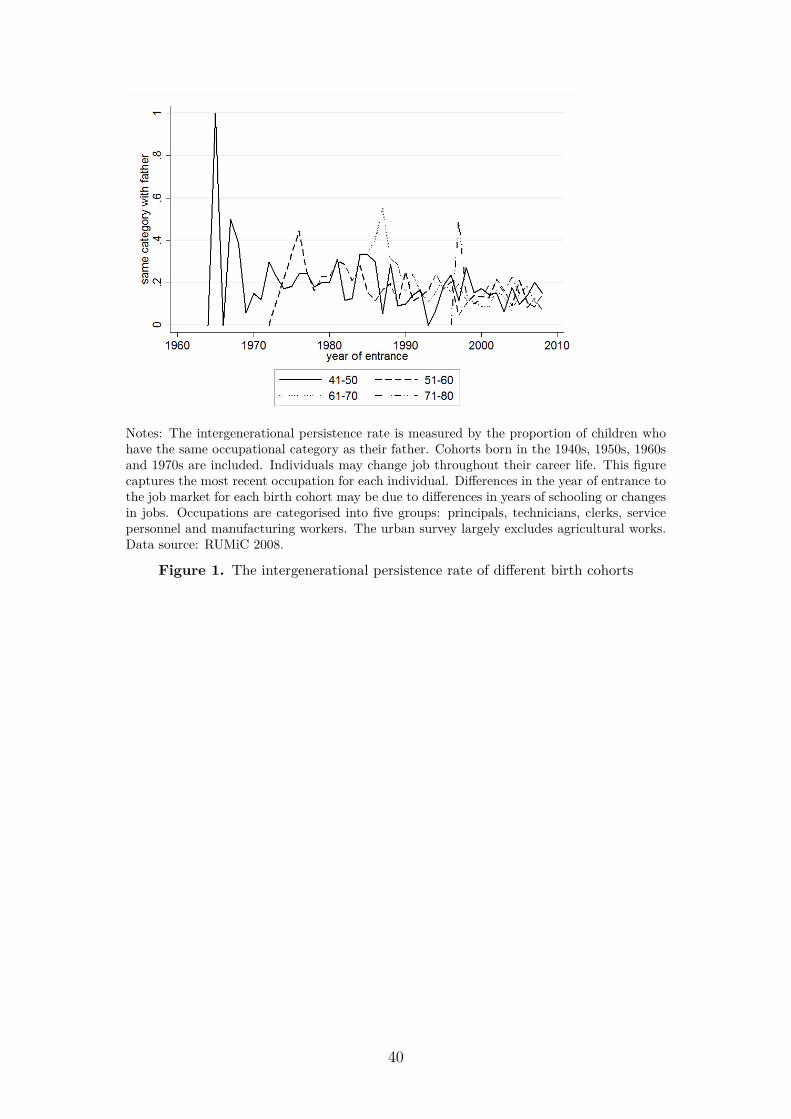
Notes: The intergenerational persistence rate is measured by the proportion of children whohave the same occupational category as their father. Cohorts born in the 1940s, 1950s, 1960sand 1970s are included. Individuals may change job throughout their career life. This figurecaptures the most recent occupation for each individual. Differences in the year of entrance tothe job market for each birth cohort may be due to differences in years of schooling or changesin jobs. Occupations are categorised into five groups: principals, technicians, clerks, servicepersonnel and manufacturing workers. The urban survey largely excludes agricultural works.Data source: RUMiC 2008.

Figure 1. The intergenerational persistence rate of different birth cohorts

40

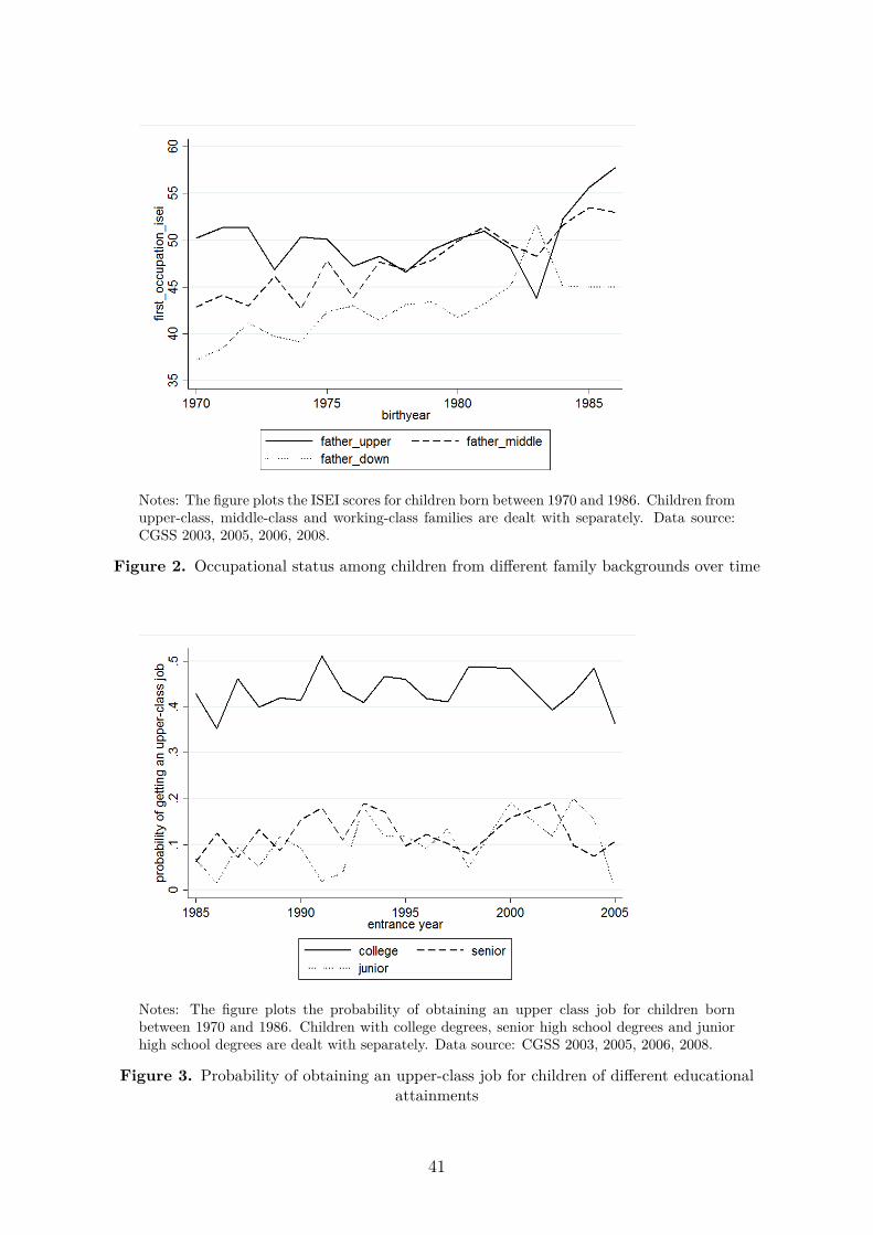
Notes: The figure plots the ISEI scores for children born between 1970 and 1986. Children fromupper-class, middle-class and working-class families are dealt with separately. Data source:CGSS 2003, 2005, 2006, 2008.

Figure 2. Occupational status among children from different family backgrounds over time

Notes: The figure plots the probability of obtaining an upper class job for children bornbetween 1970 and 1986. Children with college degrees, senior high school degrees and juniorhigh school degrees are dealt with separately. Data source: CGSS 2003, 2005, 2006, 2008.

Figure 3. Probability of obtaining an upper-class job for children of different educationalattainments

41

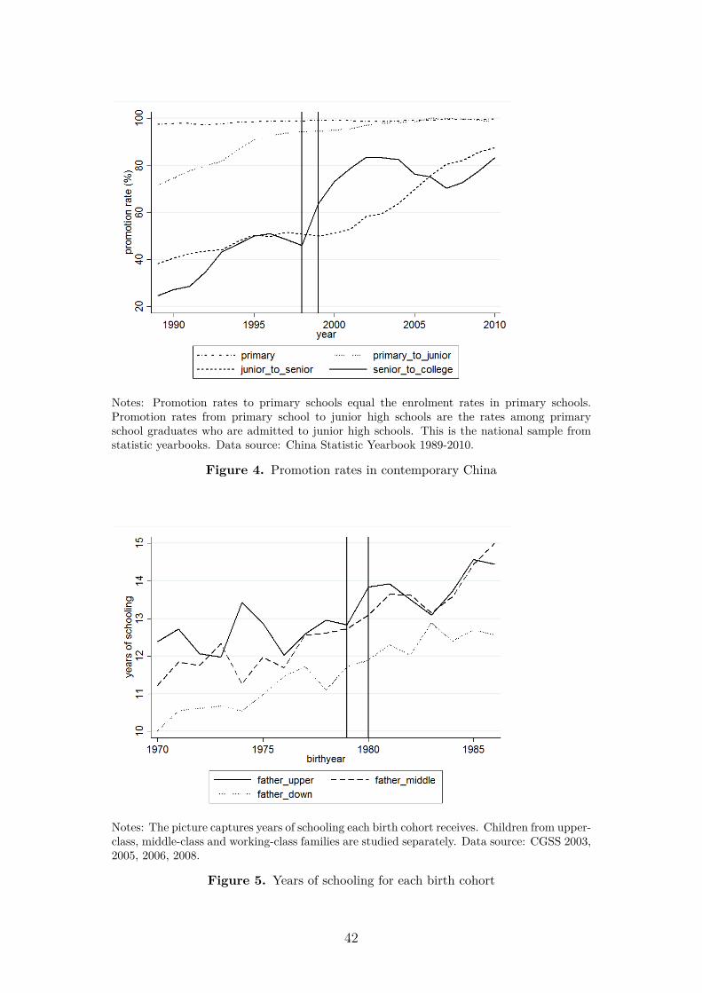
Notes: Promotion rates to primary schools equal the enrolment rates in primary schools.Promotion rates from primary school to junior high schools are the rates among primaryschool graduates who are admitted to junior high schools. This is the national sample fromstatistic yearbooks. Data source: China Statistic Yearbook 1989-2010.

Figure 4. Promotion rates in contemporary China

Notes: The picture captures years of schooling each birth cohort receives. Children from upper-class, middle-class and working-class families are studied separately. Data source: CGSS 2003,2005, 2006, 2008.

Figure 5. Years of schooling for each birth cohort

42

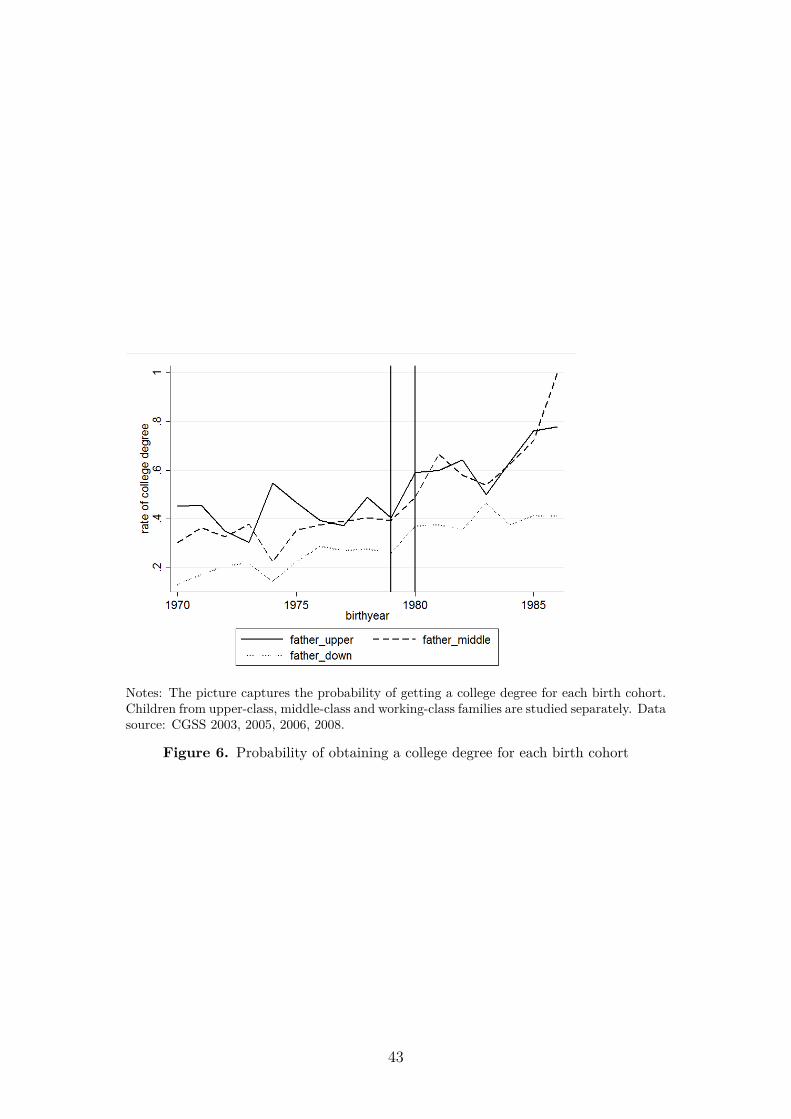
Notes: The picture captures the probability of getting a college degree for each birth cohort.Children from upper-class, middle-class and working-class families are studied separately. Datasource: CGSS 2003, 2005, 2006, 2008.

Figure 6. Probability of obtaining a college degree for each birth cohort

43

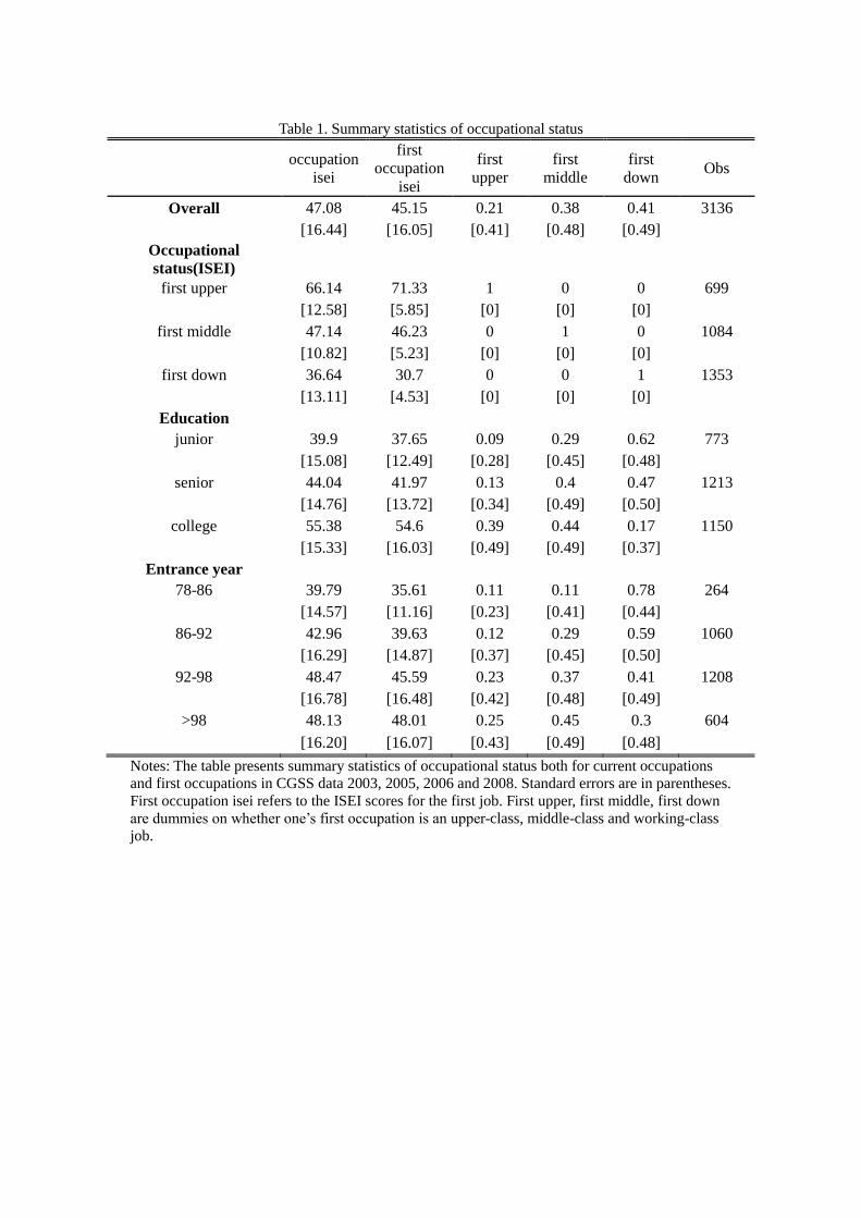
Table 1. Summary statistics of occupational status

occupation

isei

first

occupation

isei

first

upper

first

middle

first

down Obs

Overall 47.08 45.15 0.21 0.38 0.41 3136

[16.44] [16.05] [0.41] [0.48] [0.49]

Occupational

status(ISEI)

first upper 66.14 71.33 1 0 0 699

[12.58] [5.85] [0] [0] [0]

first middle 47.14 46.23 0 1 0 1084

[10.82] [5.23] [0] [0] [0]

first down 36.64 30.7 0 0 1 1353

[13.11] [4.53] [0] [0] [0]

Education

junior 39.9 37.65 0.09 0.29 0.62 773

[15.08] [12.49] [0.28] [0.45] [0.48]

senior 44.04 41.97 0.13 0.4 0.47 1213

[14.76] [13.72] [0.34] [0.49] [0.50]

college 55.38 54.6 0.39 0.44 0.17 1150

[15.33] [16.03] [0.49] [0.49] [0.37]

Entrance year

78-86 39.79 35.61 0.11 0.11 0.78 264

[14.57] [11.16] [0.23] [0.41] [0.44]

86-92 42.96 39.63 0.12 0.29 0.59 1060

[16.29] [14.87] [0.37] [0.45] [0.50]

92-98 48.47 45.59 0.23 0.37 0.41 1208

[16.78] [16.48] [0.42] [0.48] [0.49]

>98 48.13 48.01 0.25 0.45 0.3 604

[16.20] [16.07] [0.43] [0.49] [0.48]

Notes: The table presents summary statistics of occupational status both for current occupations

and first occupations in CGSS data 2003, 2005, 2006 and 2008. Standard errors are in parentheses.

First occupation isei refers to the ISEI scores for the first job. First upper, first middle, first down

are dummies on whether one’s first occupation is an upper-class, middle-class and working-class

job.

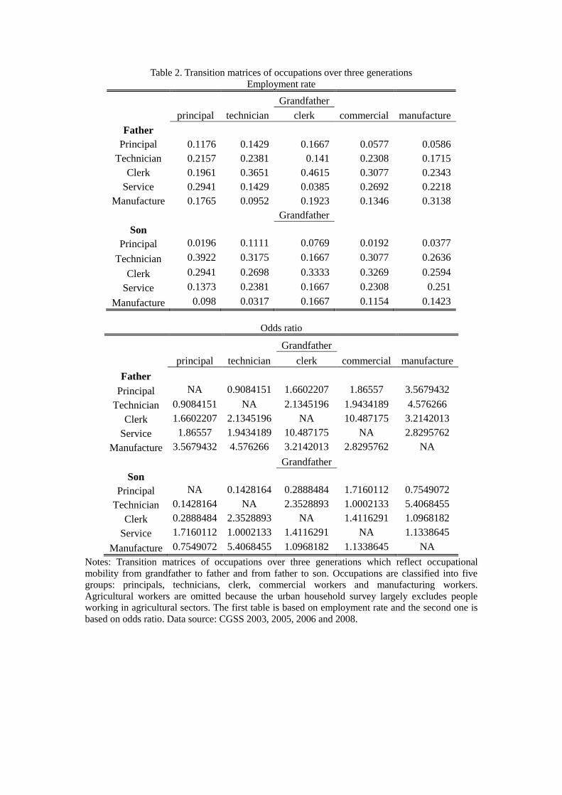
Table 2. Transition matrices of occupations over three generations

Employment rate

Grandfather

principal technician clerk commercial manufacture

Father

Principal 0.1176 0.1429 0.1667 0.0577 0.0586

Technician 0.2157 0.2381 0.141 0.2308 0.1715

Clerk 0.1961 0.3651 0.4615 0.3077 0.2343

Service 0.2941 0.1429 0.0385 0.2692 0.2218

Manufacture 0.1765 0.0952 0.1923 0.1346 0.3138

Grandfather

Son

Principal 0.0196 0.1111 0.0769 0.0192 0.0377

Technician 0.3922 0.3175 0.1667 0.3077 0.2636

Clerk 0.2941 0.2698 0.3333 0.3269 0.2594

Service 0.1373 0.2381 0.1667 0.2308 0.251

Manufacture 0.098 0.0317 0.1667 0.1154 0.1423

Odds ratio

Grandfather

principal technician clerk commercial manufacture

Father

Principal NA 0.9084151 1.6602207 1.86557 3.5679432

Technician 0.9084151 NA 2.1345196 1.9434189 4.576266

Clerk 1.6602207 2.1345196 NA 10.487175 3.2142013

Service 1.86557 1.9434189 10.487175 NA 2.8295762

Manufacture 3.5679432 4.576266 3.2142013 2.8295762 NA

Grandfather

Son

Principal NA 0.1428164 0.2888484 1.7160112 0.7549072

Technician 0.1428164 NA 2.3528893 1.0002133 5.4068455

Clerk 0.2888484 2.3528893 NA 1.4116291 1.0968182

Service 1.7160112 1.0002133 1.4116291 NA 1.1338645

Manufacture 0.7549072 5.4068455 1.0968182 1.1338645 NA

Notes: Transition matrices of occupations over three generations which reflect occupational

mobility from grandfather to father and from father to son. Occupations are classified into five

groups: principals, technicians, clerk, commercial workers and manufacturing workers.

Agricultural workers are omitted because the urban household survey largely excludes people

working in agricultural sectors. The first table is based on employment rate and the second one is

based on odds ratio. Data source: CGSS 2003, 2005, 2006 and 2008.

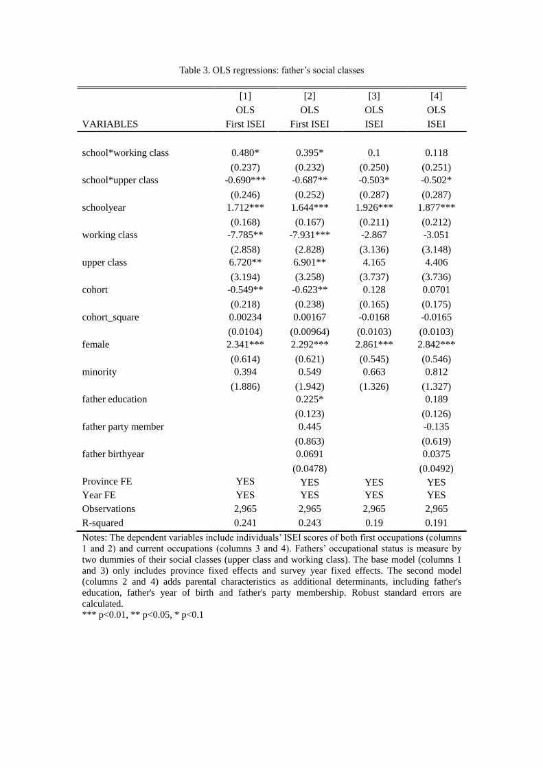
Table 3. OLS regressions: father’s social classes

[1] [2] [3] [4]

OLS OLS OLS OLS

VARIABLES First ISEI First ISEI ISEI ISEI

school*working class 0.480* 0.395* 0.1 0.118

(0.237) (0.232) (0.250) (0.251)

school*upper class -0.690*** -0.687** -0.503* -0.502*

(0.246) (0.252) (0.287) (0.287)

schoolyear 1.712*** 1.644*** 1.926*** 1.877***

(0.168) (0.167) (0.211) (0.212)

working class -7.785** -7.931*** -2.867 -3.051

(2.858) (2.828) (3.136) (3.148)

upper class 6.720** 6.901** 4.165 4.406

(3.194) (3.258) (3.737) (3.736)

cohort -0.549** -0.623** 0.128 0.0701

(0.218) (0.238) (0.165) (0.175)

cohort_square 0.00234 0.00167 -0.0168 -0.0165

(0.0104) (0.00964) (0.0103) (0.0103)

female 2.341*** 2.292*** 2.861*** 2.842***

(0.614) (0.621) (0.545) (0.546)

minority 0.394 0.549 0.663 0.812

(1.886) (1.942) (1.326) (1.327)

father education 0.225*

0.189

(0.123)

(0.126)

father party member 0.445

-0.135

(0.863)

(0.619)

father birthyear 0.0691

0.0375

(0.0478)

(0.0492)

Province FE YES YES YES YES

Year FE YES YES YES YES

Observations 2,965 2,965 2,965 2,965

R-squared 0.241 0.243 0.19 0.191

Notes: The dependent variables include individuals’ ISEI scores of both first occupations (columns

1 and 2) and current occupations (columns 3 and 4). Fathers’ occupational status is measure by

two dummies of their social classes (upper class and working class). The base model (columns 1

and 3) only includes province fixed effects and survey year fixed effects. The second model

(columns 2 and 4) adds parental characteristics as additional determinants, including father's

education, father's year of birth and father's party membership. Robust standard errors are

calculated.

*** p<0.01, ** p<0.05, * p<0.1

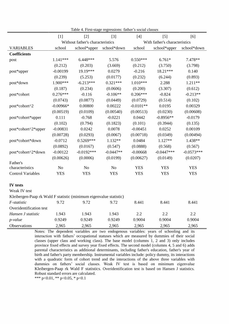
Table 4. First-stage regressions: father’s social classes

[1] [2] [3] [4] [5] [6]

Without father's characteristics With father's characteristics

VARIABLES school school*upper school*down school school*upper school*down

Coefficients

post 1.141*** 6.448*** 5.576 0.550*** 6.761* 7.478**

(0.212) (0.203) (3.669) (0.212) (3.750) (3.798)

post*upper -0.00199 19.19*** 0.0279 -0.216 18.21*** 0.140

(0.239) (5.253) (0.0177) (0.232) (6.244) (0.893)

post*down 1.900*** -6.213*** 0.321*** 1.010*** 2.288 1.211**

(0.187) (0.234) (0.0606) (0.200) (3.307) (0.612)

post*cohort 0.276*** -0.116 -0.106** 0.206*** -0.824 -0.213**

(0.0743) (0.0877) (0.0449) (0.0729) (0.514) (0.102)

post*cohort^2 -0.00966* 0.00800 0.00222 -0.0101** 0.0195 0.00329

(0.00519) (0.0109) (0.00540) (0.00513) (0.0230) (0.00608)

post*cohort*upper 0.111 -0.768 -0.0221 0.0442 -0.8956** -0.0179

(0.102) (0.794) (0.1823) (0.101) (0.3944) (0.135)

post*cohort^2*upper -0.00831 0.0242 0.0078 -0.00451 0.0252 0.00109

(0.00728) (0.0293) (0.0067) (0.00718) (0.0349) (0.00494)

post*cohort*down -0.0712 0.5269*** 1.132** 0.0484 1.127** 1.438**

(0.0892) (0.0167) (0.547) (0.0888) (0.568) (0.567)

post*cohort^2*down -0.00122 -0.0192*** -0.0447** -0.00668 -0.0447*** -0.0573***

(0.00626) (0.0006) (0.0199) (0.00627) (0.0149) (0.0207)

Father's

characteristics No No No YES YES YES

Control Variables YES YES YES YES YES YES

IV tests

Weak IV test

Kleibergen-Paap rk Wald F statistic (minimum eigenvalue statistic)

F-statistic 9.72 9.72 9.72 8.441 8.441 8.441

Overidentification test

Hansen J statistic 1.943 1.943 1.943 2.2 2.2 2.2

p-value 0.9249 0.9249 0.9249 0.9004 0.9004 0.9004

Observations 2,965 2,965 2,965 2,965 2,965 2,965

Notes: The dependent variables are two endogenous variables: years of schooling and its

interaction with fathers’ occupational statuses which are measured by dummies of their social

classes (upper class and working class). The base model (columns 1, 2 and 3) only includes

province fixed effects and survey year fixed effects. The second model (columns 4, 5 and 6) adds

parental characteristics as additional determinants, including father's education, father's year of

birth and father's party membership. Instrumental variables include: policy dummy, its interactions

with a quadratic form of cohort trend and the interactions of the above three variables with

dummies on fathers’ social classes. Weak IV test is based on minimum eigenvalue

Kleibergen-Paap rk Wald F statistics. Overidentification test is based on Hansen J statistics.

Robust standard errors are calculated.

*** p<0.01, ** p<0.05, * p<0.1

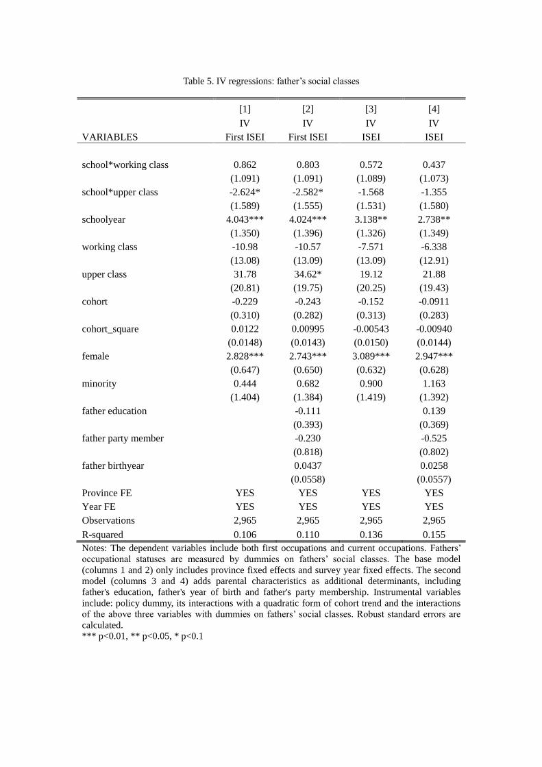
Table 5. IV regressions: father’s social classes

[1] [2] [3] [4]

IV IV IV IV

VARIABLES First ISEI First ISEI ISEI ISEI

school*working class 0.862 0.803 0.572 0.437

(1.091) (1.091) (1.089) (1.073)

school*upper class -2.624* -2.582* -1.568 -1.355

(1.589) (1.555) (1.531) (1.580)

schoolyear 4.043*** 4.024*** 3.138** 2.738**

(1.350) (1.396) (1.326) (1.349)

working class -10.98 -10.57 -7.571 -6.338

(13.08) (13.09) (13.09) (12.91)

upper class 31.78 34.62* 19.12 21.88

(20.81) (19.75) (20.25) (19.43)

cohort -0.229 -0.243 -0.152 -0.0911

(0.310) (0.282) (0.313) (0.283)

cohort_square 0.0122 0.00995 -0.00543 -0.00940

(0.0148) (0.0143) (0.0150) (0.0144)

female 2.828*** 2.743*** 3.089*** 2.947***

(0.647) (0.650) (0.632) (0.628)

minority 0.444 0.682 0.900 1.163

(1.404) (1.384) (1.419) (1.392)

father education

-0.111

0.139

(0.393)

(0.369)

father party member

-0.230

-0.525

(0.818)

(0.802)

father birthyear

0.0437

0.0258

(0.0558)

(0.0557)

Province FE YES YES YES YES

Year FE YES YES YES YES

Observations 2,965 2,965 2,965 2,965

R-squared 0.106 0.110 0.136 0.155

Notes: The dependent variables include both first occupations and current occupations. Fathers’

occupational statuses are measured by dummies on fathers’ social classes. The base model

(columns 1 and 2) only includes province fixed effects and survey year fixed effects. The second

model (columns 3 and 4) adds parental characteristics as additional determinants, including

father's education, father's year of birth and father's party membership. Instrumental variables

include: policy dummy, its interactions with a quadratic form of cohort trend and the interactions

of the above three variables with dummies on fathers’ social classes. Robust standard errors are

calculated.

*** p<0.01, ** p<0.05, * p<0.1

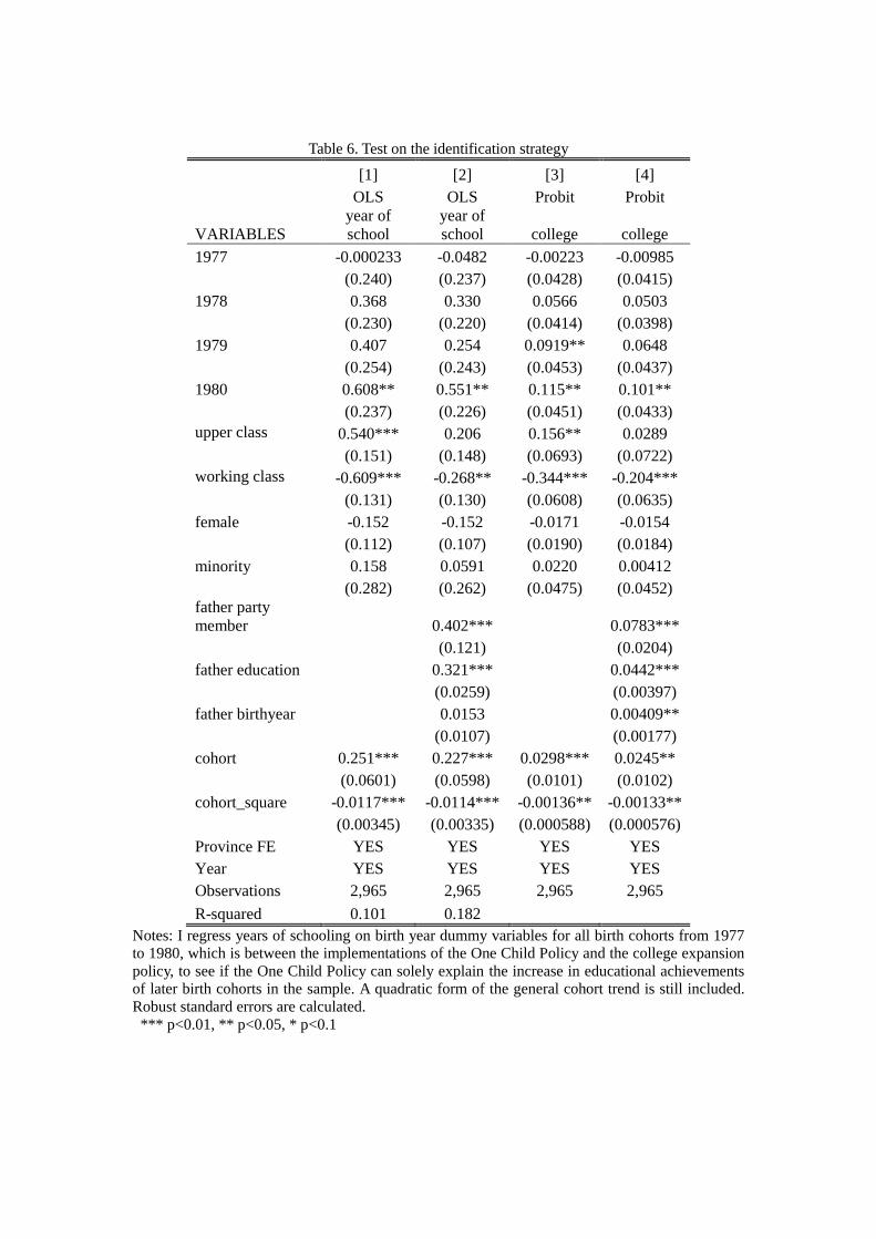
Table 6. Test on the identification strategy

[1] [2] [3] [4]

OLS OLS Probit Probit

VARIABLES

year of

school

year of

school college college

1977 -0.000233 -0.0482 -0.00223 -0.00985

(0.240) (0.237) (0.0428) (0.0415)

1978 0.368 0.330 0.0566 0.0503

(0.230) (0.220) (0.0414) (0.0398)

1979 0.407 0.254 0.0919** 0.0648

(0.254) (0.243) (0.0453) (0.0437)

1980 0.608** 0.551** 0.115** 0.101**

(0.237) (0.226) (0.0451) (0.0433)

upper class 0.540*** 0.206 0.156** 0.0289

(0.151) (0.148) (0.0693) (0.0722)

working class -0.609*** -0.268** -0.344*** -0.204***

(0.131) (0.130) (0.0608) (0.0635)

female -0.152 -0.152 -0.0171 -0.0154

(0.112) (0.107) (0.0190) (0.0184)

minority 0.158 0.0591 0.0220 0.00412

(0.282) (0.262) (0.0475) (0.0452)

father party

member

0.402***

0.0783***

(0.121)

(0.0204)

father education

0.321***

0.0442***

(0.0259)

(0.00397)

father birthyear

0.0153

0.00409**

(0.0107)

(0.00177)

cohort 0.251*** 0.227*** 0.0298*** 0.0245**

(0.0601) (0.0598) (0.0101) (0.0102)

cohort_square -0.0117*** -0.0114*** -0.00136** -0.00133**

(0.00345) (0.00335) (0.000588) (0.000576)

Province FE YES YES YES YES

Year YES YES YES YES

Observations 2,965 2,965 2,965 2,965

R-squared 0.101 0.182

Notes: I regress years of schooling on birth year dummy variables for all birth cohorts from 1977

to 1980, which is between the implementations of the One Child Policy and the college expansion

policy, to see if the One Child Policy can solely explain the increase in educational achievements

of later birth cohorts in the sample. A quadratic form of the general cohort trend is still included.

Robust standard errors are calculated.

*** p<0.01, ** p<0.05, * p<0.1

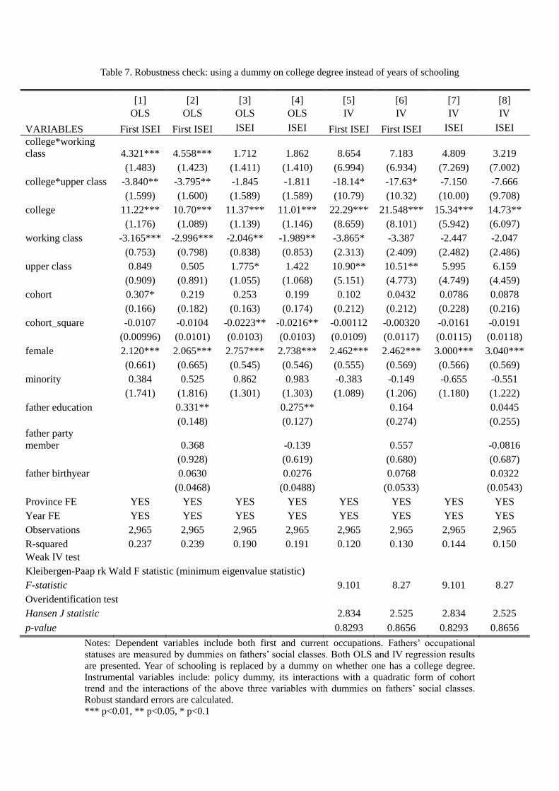
Table 7. Robustness check: using a dummy on college degree instead of years of schooling

[1] [2] [3] [4] [5] [6] [7] [8]

OLS OLS OLS OLS IV IV IV IV

VARIABLES First ISEI First ISEI ISEI ISEI First ISEI First ISEI ISEI ISEI

college*working

class 4.321*** 4.558*** 1.712 1.862 8.654 7.183 4.809 3.219

(1.483) (1.423) (1.411) (1.410) (6.994) (6.934) (7.269) (7.002)

college*upper class -3.840** -3.795** -1.845 -1.811 -18.14* -17.63* -7.150 -7.666

(1.599) (1.600) (1.589) (1.589) (10.79) (10.32) (10.00) (9.708)

college 11.22*** 10.70*** 11.37*** 11.01*** 22.29*** 21.548*** 15.34*** 14.73**

(1.176) (1.089) (1.139) (1.146) (8.659) (8.101) (5.942) (6.097)

working class -3.165*** -2.996*** -2.046** -1.989** -3.865* -3.387 -2.447 -2.047

(0.753) (0.798) (0.838) (0.853) (2.313) (2.409) (2.482) (2.486)

upper class 0.849 0.505 1.775* 1.422 10.90** 10.51** 5.995 6.159

(0.909) (0.891) (1.055) (1.068) (5.151) (4.773) (4.749) (4.459)

cohort 0.307* 0.219 0.253 0.199 0.102 0.0432 0.0786 0.0878

(0.166) (0.182) (0.163) (0.174) (0.212) (0.212) (0.228) (0.216)

cohort_square -0.0107 -0.0104 -0.0223** -0.0216** -0.00112 -0.00320 -0.0161 -0.0191

(0.00996) (0.0101) (0.0103) (0.0103) (0.0109) (0.0117) (0.0115) (0.0118)

female 2.120*** 2.065*** 2.757*** 2.738*** 2.462*** 2.462*** 3.000*** 3.040***

(0.661) (0.665) (0.545) (0.546) (0.555) (0.569) (0.566) (0.569)

minority 0.384 0.525 0.862 0.983 -0.383 -0.149 -0.655 -0.551

(1.741) (1.816) (1.301) (1.303) (1.089) (1.206) (1.180) (1.222)

father education

0.331**

0.275**

0.164

0.0445

(0.148)

(0.127)

(0.274)

(0.255)

father party

member

0.368 -0.139

0.557

-0.0816

(0.928)

(0.619)

(0.680)

(0.687)

father birthyear

0.0630

0.0276

0.0768

0.0322

(0.0468)

(0.0488)

(0.0533)

(0.0543)

Province FE YES YES YES YES YES YES YES YES

Year FE YES YES YES YES YES YES YES YES

Observations 2,965 2,965 2,965 2,965 2,965 2,965 2,965 2,965

R-squared 0.237 0.239 0.190 0.191 0.120 0.130 0.144 0.150

Weak IV test

Kleibergen-Paap rk Wald F statistic (minimum eigenvalue statistic)

F-statistic

9.101 8.27 9.101 8.27

Overidentification test

Hansen J statistic

2.834 2.525 2.834 2.525

p-value 0.8293 0.8656 0.8293 0.8656

Notes: Dependent variables include both first and current occupations. Fathers’ occupational

statuses are measured by dummies on fathers’ social classes. Both OLS and IV regression results

are presented. Year of schooling is replaced by a dummy on whether one has a college degree.

Instrumental variables include: policy dummy, its interactions with a quadratic form of cohort

trend and the interactions of the above three variables with dummies on fathers’ social classes. Robust standard errors are calculated.

*** p<0.01, ** p<0.05, * p<0.1

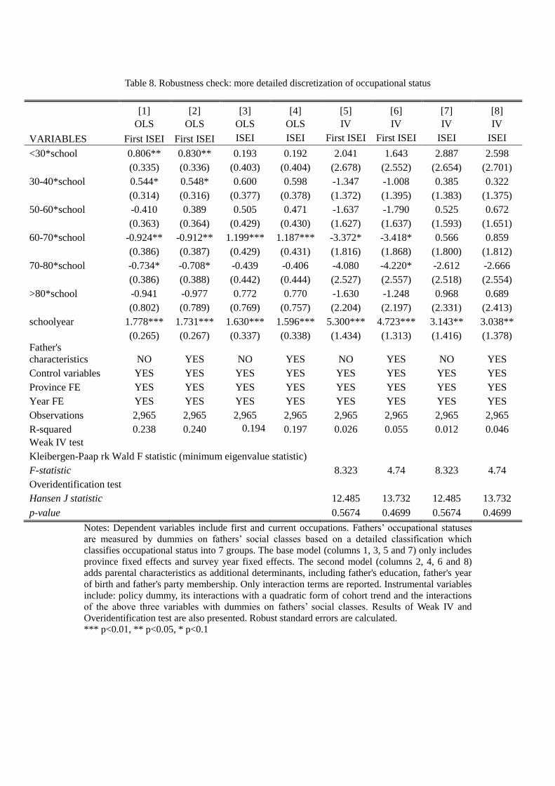
Table 8. Robustness check: more detailed discretization of occupational status

[1] [2] [3] [4] [5] [6] [7] [8]

OLS OLS OLS OLS IV IV IV IV

VARIABLES First ISEI First ISEI ISEI ISEI First ISEI First ISEI ISEI ISEI

<30*school 0.806** 0.830** 0.193 0.192 2.041 1.643 2.887 2.598

(0.335) (0.336) (0.403) (0.404) (2.678) (2.552) (2.654) (2.701)

30-40*school 0.544* 0.548* 0.600 0.598 -1.347 -1.008 0.385 0.322

(0.314) (0.316) (0.377) (0.378) (1.372) (1.395) (1.383) (1.375)

50-60*school -0.410 0.389 0.505 0.471 -1.637 -1.790 0.525 0.672

(0.363) (0.364) (0.429) (0.430) (1.627) (1.637) (1.593) (1.651)

60-70*school -0.924** -0.912** 1.199*** 1.187*** -3.372* -3.418* 0.566 0.859

(0.386) (0.387) (0.429) (0.431) (1.816) (1.868) (1.800) (1.812)

70-80*school -0.734* -0.708* -0.439 -0.406 -4.080 -4.220* -2.612 -2.666

(0.386) (0.388) (0.442) (0.444) (2.527) (2.557) (2.518) (2.554)

>80*school -0.941 -0.977 0.772 0.770 -1.630 -1.248 0.968 0.689

(0.802) (0.789) (0.769) (0.757) (2.204) (2.197) (2.331) (2.413)

schoolyear 1.778*** 1.731*** 1.630*** 1.596*** 5.300*** 4.723*** 3.143** 3.038**

(0.265) (0.267) (0.337) (0.338) (1.434) (1.313) (1.416) (1.378)

Father's

characteristics NO YES NO YES NO YES NO YES

Control variables YES YES YES YES YES YES YES YES

Province FE YES YES YES YES YES YES YES YES

Year FE YES YES YES YES YES YES YES YES

Observations 2,965 2,965 2,965 2,965 2,965 2,965 2,965 2,965

R-squared 0.238 0.240 0.194 0.197 0.026 0.055 0.012 0.046

Weak IV test

Kleibergen-Paap rk Wald F statistic (minimum eigenvalue statistic)

F-statistic

8.323 4.74 8.323 4.74

Overidentification test

Hansen J statistic

12.485 13.732 12.485 13.732

p-value 0.5674 0.4699 0.5674 0.4699

Notes: Dependent variables include first and current occupations. Fathers’ occupational statuses

are measured by dummies on fathers’ social classes based on a detailed classification which

classifies occupational status into 7 groups. The base model (columns 1, 3, 5 and 7) only includes

province fixed effects and survey year fixed effects. The second model (columns 2, 4, 6 and 8)

adds parental characteristics as additional determinants, including father's education, father's year

of birth and father's party membership. Only interaction terms are reported. Instrumental variables

include: policy dummy, its interactions with a quadratic form of cohort trend and the interactions

of the above three variables with dummies on fathers’ social classes. Results of Weak IV and

Overidentification test are also presented. Robust standard errors are calculated.

*** p<0.01, ** p<0.05, * p<0.1

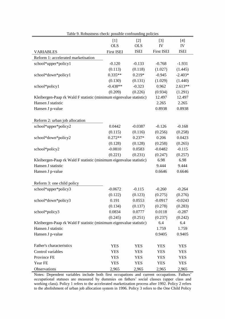
Table 9. Robustness check: possible confounding policies

[1] [2] [3] [4]

OLS OLS IV IV

VARIABLES First ISEI ISEI First ISEI ISEI

Reform 1: accelerated marketisation

school*upper*policy1 -0.120 -0.133 -0.768 -1.931

(0.113) (0.118) (1.027) (1.445)

school*down*policy1 0.335** 0.219* -0.945 -2.403*

(0.130) (0.131) (1.029) (1.440)

school*policy1 -0.438** -0.323 0.962 2.613**

(0.209) (0.226) (0.934) (1.291)

Kleibergen-Paap rk Wald F statistic (minimum eigenvalue statistic) 12.497 12.497

Hansen J statistic

2.265 2.265

Hansen J p-value

0.8938 0.8938

Reform 2: urban job allocation

school*upper*policy2 0.0442 -0.0387 -0.126 -0.168

(0.115) (0.116) (0.256) (0.258)

school*down*policy2 0.272** 0.237* 0.206 0.0423

(0.128) (0.128) (0.258) (0.265)

school*policy2 -0.0810 0.0583 -0.0482 -0.115

(0.221) (0.231) (0.247) (0.257)

Kleibergen-Paap rk Wald F statistic (minimum eigenvalue statistic) 6.98 6.98

Hansen J statistic

9.444 9.444

Hansen J p-value

0.6646 0.6646

Reform 3: one child policy

school*upper*policy3 -0.0672 -0.115 -0.260 -0.264

(0.122) (0.123) (0.275) (0.276)

school*down*policy3 0.191 0.0553 -0.0917 -0.0243

(0.134) (0.137) (0.278) (0.283)

school*policy3 0.0834 0.0777 0.0118 -0.287

(0.245) (0.251) (0.237) (0.242)

Kleibergen-Paap rk Wald F statistic (minimum eigenvalue statistic) 6.4 6.4

Hansen J statistic

1.759 1.759

Hansen J p-value

0.9405 0.9405

Father's characteristics YES YES YES YES

Control variables YES YES YES YES

Province FE YES YES YES YES

Year FE YES YES YES YES

Observations 2,965 2,965 2,965 2,965

Notes: Dependent variables include both first occupations and current occupations. Fathers’

occupational statuses are measured by dummies on fathers’ social classes (upper class and working class). Policy 1 refers to the accelerated marketization process after 1992. Policy 2 refers

to the abolishment of urban job allocation system in 1996. Policy 3 refers to the One Child Policy

after 1979. Only interaction terms are reported. All the models include province fixed effects,

survey year fixed effects and parental characteristics, including father's education, father's year of

birth and father's party membership. Instrumental variables include: policy dummy, its interactions

with a quadratic form of cohort trend and the interactions of the above three variables with

dummies on fathers’ social classes. Results of Weak IV and Overidentification test are also

presented. Robust standard errors are calculated.

*** p<0.01, ** p<0.05, * p<0.1

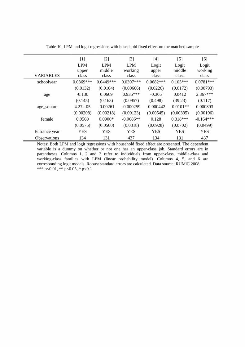
Table 10. LPM and logit regressions with household fixed effect on the matched sample

[1] [2] [3] [4] [5] [6]

LPM LPM LPM Logit Logit Logit

VARIABLES

upper

class

middle

class

working

class

upper

class

middle

class

working

class

schoolyear 0.0369*** 0.0449*** 0.0397*** 0.0682*** 0.105*** 0.0781***

(0.0132) (0.0104) (0.00606) (0.0226) (0.0172) (0.00793)

age -0.130 0.0669 0.935*** -0.305 0.0412 2.367***

(0.145) (0.163) (0.0957) (0.498) (39.23) (0.117)

age_square 4.27e-05 -0.00261 -0.000259 -0.000442 -0.0101** 0.000893

(0.00208) (0.00218) (0.00123) (0.00545) (0.00395) (0.00196)

female 0.0560 0.0900* -0.0686** 0.128 0.318*** -0.164***

(0.0575) (0.0500) (0.0318) (0.0928) (0.0702) (0.0499)

Entrance year YES YES YES YES YES YES

Observations 134 131 437 134 131 437

Notes: Both LPM and logit regressions with household fixed effect are presented. The dependent

variable is a dummy on whether or not one has an upper-class job. Standard errors are in

parentheses. Columns 1, 2 and 3 refer to individuals from upper-class, middle-class and

working-class families with LPM (linear probability model). Columns 4, 5, and 6 are

corresponding logit models. Robust standard errors are calculated. Data source: RUMiC 2008.

*** p<0.01, ** p<0.05, * p<0.1

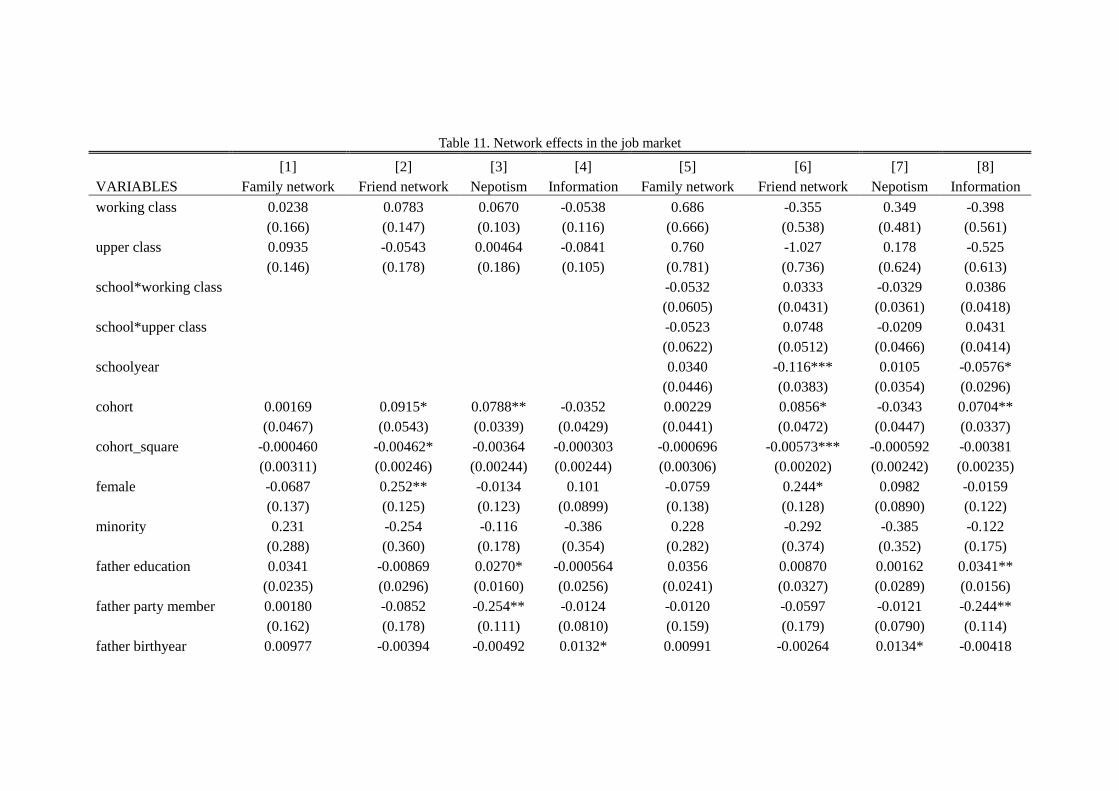
Table 11. Network effects in the job market

[1] [2] [3] [4] [5] [6] [7] [8]

VARIABLES Family network Friend network Nepotism Information Family network Friend network Nepotism Information

working class 0.0238 0.0783 0.0670 -0.0538 0.686 -0.355 0.349 -0.398

(0.166) (0.147) (0.103) (0.116) (0.666) (0.538) (0.481) (0.561)

upper class 0.0935 -0.0543 0.00464 -0.0841 0.760 -1.027 0.178 -0.525

(0.146) (0.178) (0.186) (0.105) (0.781) (0.736) (0.624) (0.613)

school*working class

-0.0532 0.0333 -0.0329 0.0386

(0.0605) (0.0431) (0.0361) (0.0418)

school*upper class

-0.0523 0.0748 -0.0209 0.0431

(0.0622) (0.0512) (0.0466) (0.0414)

schoolyear

0.0340 -0.116*** 0.0105 -0.0576*

(0.0446) (0.0383) (0.0354) (0.0296)

cohort 0.00169 0.0915* 0.0788** -0.0352 0.00229 0.0856* -0.0343 0.0704**

(0.0467) (0.0543) (0.0339) (0.0429) (0.0441) (0.0472) (0.0447) (0.0337)

cohort_square -0.000460 -0.00462* -0.00364 -0.000303 -0.000696 -0.00573*** -0.000592 -0.00381

(0.00311) (0.00246) (0.00244) (0.00244) (0.00306) (0.00202) (0.00242) (0.00235)

female -0.0687 0.252** -0.0134 0.101 -0.0759 0.244* 0.0982 -0.0159

(0.137) (0.125) (0.123) (0.0899) (0.138) (0.128) (0.0890) (0.122)

minority 0.231 -0.254 -0.116 -0.386 0.228 -0.292 -0.385 -0.122

(0.288) (0.360) (0.178) (0.354) (0.282) (0.374) (0.352) (0.175)

father education 0.0341 -0.00869 0.0270* -0.000564 0.0356 0.00870 0.00162 0.0341**

(0.0235) (0.0296) (0.0160) (0.0256) (0.0241) (0.0327) (0.0289) (0.0156)

father party member 0.00180 -0.0852 -0.254** -0.0124 -0.0120 -0.0597 -0.0121 -0.244**

(0.162) (0.178) (0.111) (0.0810) (0.159) (0.179) (0.0790) (0.114)

father birthyear 0.00977 -0.00394 -0.00492 0.0132* 0.00991 -0.00264 0.0134* -0.00418

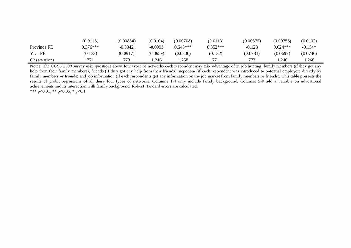
(0.0115) (0.00884) (0.0104) (0.00708) (0.0113) (0.00875) (0.00755) (0.0102)

Province FE 0.376*** -0.0942 -0.0993 0.640*** 0.352*** -0.128 0.624*** -0.134*

Year FE (0.133) (0.0917) (0.0659) (0.0800) (0.132) (0.0981) (0.0697) (0.0746)

Observations 771 773 1,246 1,268 771 773 1,246 1,268

Notes: The CGSS 2008 survey asks questions about four types of networks each respondent may take advantage of in job hunting: family members (if they got any

help from their family members), friends (if they got any help from their friends), nepotism (if each respondent was introduced to potential employers directly by

family members or friends) and job information (if each respondents got any information on the job market from family members or friends). This table presents the

results of probit regressions of all these four types of networks. Columns 1-4 only include family background. Columns 5-8 add a variable on educational

achievements and its interaction with family background. Robust standard errors are calculated.

*** p<0.01, ** p<0.05, * p<0.1

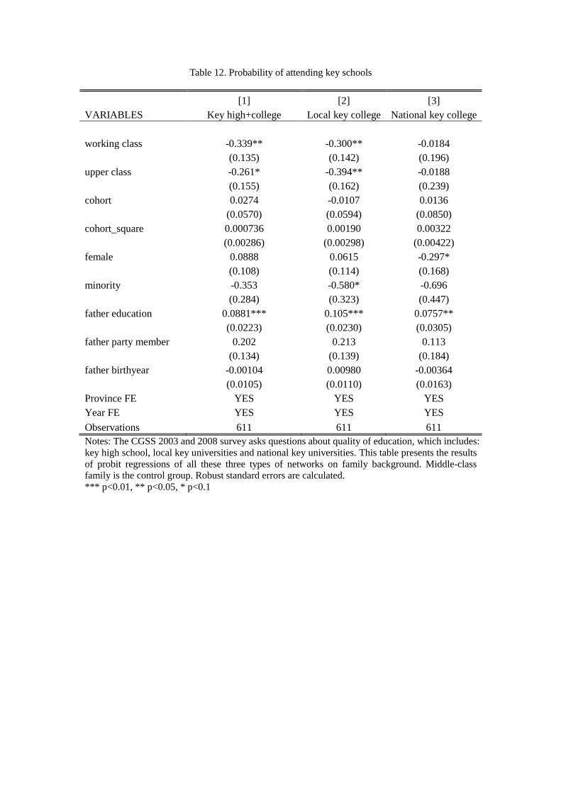
Table 12. Probability of attending key schools

[1] [2] [3]

VARIABLES Key high+college Local key college National key college

working class -0.339** -0.300** -0.0184

(0.135) (0.142) (0.196)

upper class -0.261* -0.394** -0.0188

(0.155) (0.162) (0.239)

cohort 0.0274 -0.0107 0.0136

(0.0570) (0.0594) (0.0850)

cohort_square 0.000736 0.00190 0.00322

(0.00286) (0.00298) (0.00422)

female 0.0888 0.0615 -0.297*

(0.108) (0.114) (0.168)

minority -0.353 -0.580* -0.696

(0.284) (0.323) (0.447)

father education 0.0881*** 0.105*** 0.0757**

(0.0223) (0.0230) (0.0305)

father party member 0.202 0.213 0.113

(0.134) (0.139) (0.184)

father birthyear -0.00104 0.00980 -0.00364

(0.0105) (0.0110) (0.0163)

Province FE YES YES YES

Year FE YES YES YES

Observations 611 611 611

Notes: The CGSS 2003 and 2008 survey asks questions about quality of education, which includes:

key high school, local key universities and national key universities. This table presents the results

of probit regressions of all these three types of networks on family background. Middle-class

family is the control group. Robust standard errors are calculated.

*** p<0.01, ** p<0.05, * p<0.1

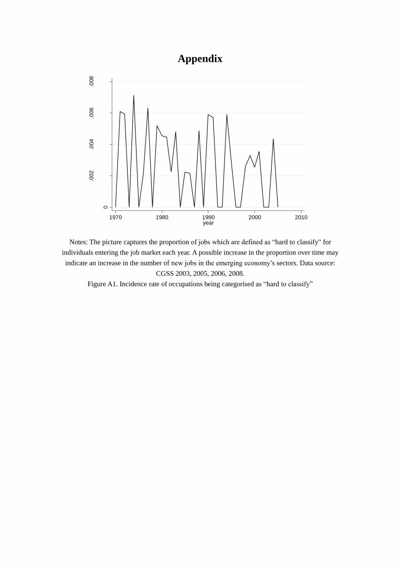
Appendix

Notes: The picture captures the proportion of jobs which are defined as “hard to classify" for

individuals entering the job market each year. A possible increase in the proportion over time may

indicate an increase in the number of new jobs in the emerging economy’s sectors. Data source:

CGSS 2003, 2005, 2006, 2008.

Figure A1. Incidence rate of occupations being categorised as “hard to classify”

0

.002

.004

.006

.008

ha

rd to

cla

ssify

1970 1980 1990 2000 2010year

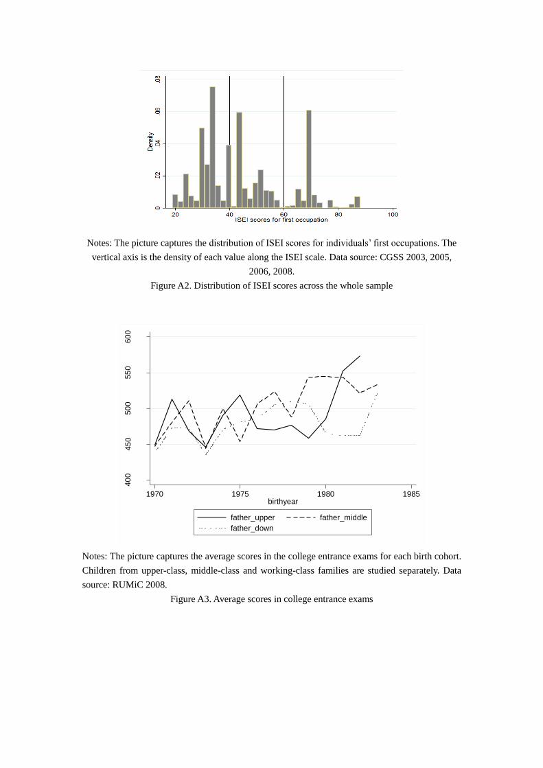
Notes: The picture captures the distribution of ISEI scores for individuals’ first occupations. The

vertical axis is the density of each value along the ISEI scale. Data source: CGSS 2003, 2005,

2006, 2008.

Figure A2. Distribution of ISEI scores across the whole sample

Notes: The picture captures the average scores in the college entrance exams for each birth cohort.

Children from upper-class, middle-class and working-class families are studied separately. Data

source: RUMiC 2008.

Figure A3. Average scores in college entrance exams

40

045

050

055

060

0

ave

rag

e e

xa

m s

co

res

1970 1975 1980 1985birthyear

father_upper father_middle

father_down

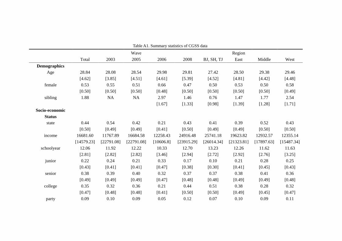
Table A1. Summary statistics of CGSS data

Wave Region

Total 2003 2005 2006 2008 BJ, SH, TJ East Middle West

Demographics

Age 28.84 28.08 28.54 29.98 29.81 27.42 28.50 29.38 29.46

[4.62] [3.85] [4.51] [4.61] [5.39] [4.52] [4.81] [4.42] [4.48]

female 0.53 0.55 0.51 0.66 0.47 0.50 0.53 0.50 0.58

[0.50] [0.50] [0.50] [0.48] [0.50] [0.50] [0.50] [0.50] [0.49]

sibling 1.88 NA NA 2.97 1.46 0.76 1.47 1.77 2.54

[1.67] [1.33] [0.98] [1.39] [1.28] [1.71]

Socio-economic

Status

state 0.44 0.54 0.42 0.21 0.43 0.41 0.39 0.52 0.43

[0.50] [0.49] [0.49] [0.41] [0.50] [0.49] [0.49] [0.50] [0.50]

income 16681.60 11767.89 16684.58 12258.43 24916.48 25741.18 19623.82 12932.57 12355.14

[14579.23] [22791.08] [22791.08] [10606.8] [23915.29] [26014.34] [21323.81] [17897.63] [15487.34]

schoolyear 12.06 11.92 12.22 10.33 12.70 13.23 12.26 11.62 11.63

[2.81] [2.82] [2.82] [3.46] [2.94] [2.72] [2.92] [2.76] [3.25]

junior 0.22 0.24 0.21 0.33 0.17 0.10 0.21 0.28 0.25

[0.43] [0.41] [0.41] [0.47] [0.38] [0.30] [0.41] [0.45] [0.43]

senior 0.38 0.39 0.40 0.32 0.37 0.37 0.38 0.41 0.36

[0.49] [0.49] [0.49] [0.47] [0.48] [0.48] [0.49] [0.49] [0.48]

college 0.35 0.32 0.36 0.21 0.44 0.51 0.38 0.28 0.32

[0.47] [0.48] [0.48] [0.41] [0.50] [0.50] [0.49] [0.45] [0.47]

party 0.09 0.10 0.09 0.05 0.12 0.07 0.10 0.09 0.11

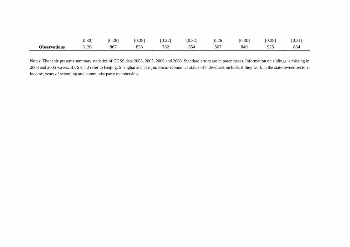
[0.30] [0.28] [0.28] [0.22] [0.32] [0.26] [0.30] [0.28] [0.31]

Observations 3136 867 833 782 654 507 840 925 864

Notes: The table presents summary statistics of CGSS data 2003, 2005, 2006 and 2008. Standard errors are in parentheses. Information on siblings is missing in

2003 and 2005 waves. BJ, SH, TJ refer to Beijing, Shanghai and Tianjin. Socio-economics status of individuals include: if they work in the state-owned sectors,

income, years of schooling and communist party membership.

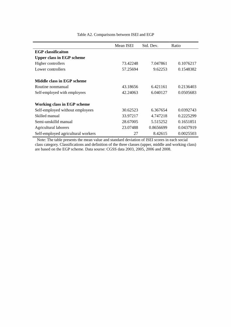
Table A2. Comparisons between ISEI and EGP

Mean ISEI Std. Dev. Ratio

EGP classificaiton

Upper class in EGP scheme

Higher controllers 73.42248 7.047861 0.1076217

Lower controllers 57.25694 9.62253 0.1548382

Middle class in EGP scheme

Routine nonmanual 43.18656 6.421161 0.2136403

Self-employed with employees 42.24063 6.040127 0.0505683

Working class in EGP scheme

Self-employed without employees 30.62523 6.367654 0.0392743

Skilled manual 33.97217 4.747218 0.2225299

Semi-unskilld manual 28.67005 5.515252 0.1651851

Agricultural laborers 23.07488 0.8656699 0.0437919

Self-employed agricultural workers 27 8.42615 0.0025503

Note: The table presents the mean value and standard deviation of ISEI scores in each social

class category. Classifications and definition of the three classes (upper, middle and working class)

are based on the EGP scheme. Data sourse: CGSS data 2003, 2005, 2006 and 2008.

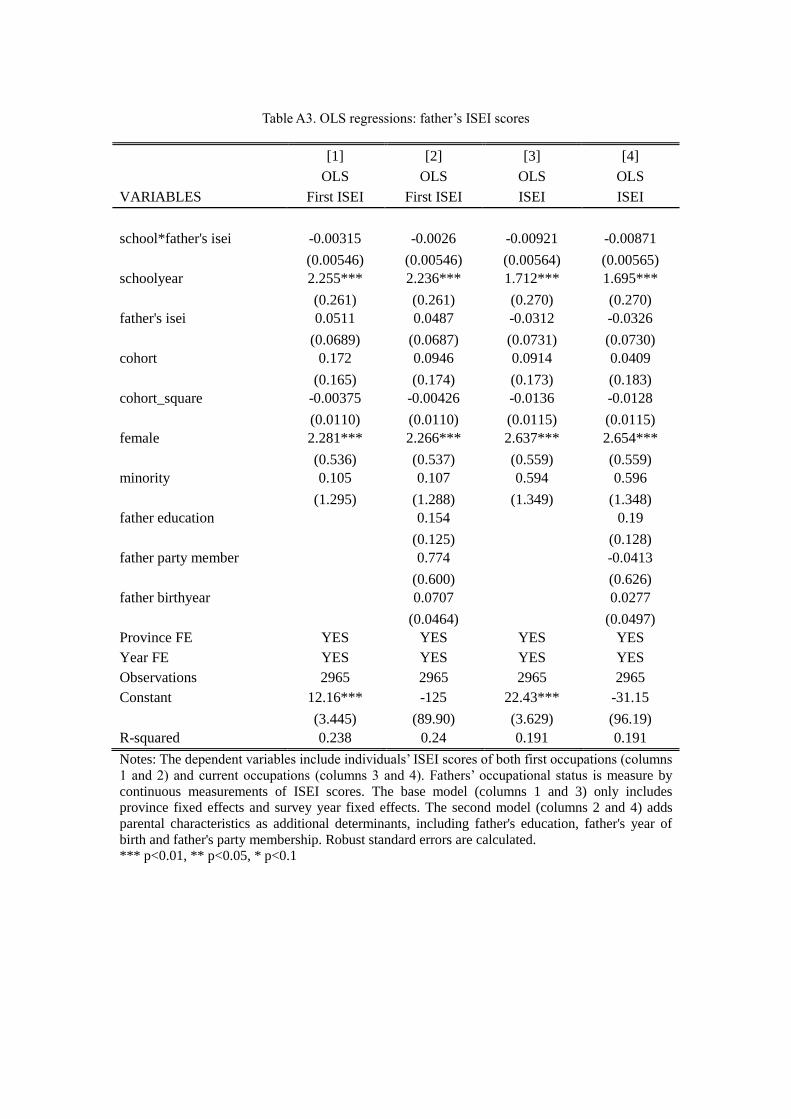
Table A3. OLS regressions: father’s ISEI scores

[1] [2] [3] [4]

OLS OLS OLS OLS

VARIABLES First ISEI First ISEI ISEI ISEI

school*father's isei -0.00315 -0.0026 -0.00921 -0.00871

(0.00546) (0.00546) (0.00564) (0.00565)

schoolyear 2.255*** 2.236*** 1.712*** 1.695***

(0.261) (0.261) (0.270) (0.270)

father's isei 0.0511 0.0487 -0.0312 -0.0326

(0.0689) (0.0687) (0.0731) (0.0730)

cohort 0.172 0.0946 0.0914 0.0409

(0.165) (0.174) (0.173) (0.183)

cohort_square -0.00375 -0.00426 -0.0136 -0.0128

(0.0110) (0.0110) (0.0115) (0.0115)

female 2.281*** 2.266*** 2.637*** 2.654***

(0.536) (0.537) (0.559) (0.559)

minority 0.105 0.107 0.594 0.596

(1.295) (1.288) (1.349) (1.348)

father education 0.154

0.19

(0.125)

(0.128)

father party member 0.774

-0.0413

(0.600)

(0.626)

father birthyear 0.0707

0.0277

(0.0464)

(0.0497)

Province FE YES YES YES YES

Year FE YES YES YES YES

Observations 2965 2965 2965 2965

Constant 12.16*** -125 22.43*** -31.15

(3.445) (89.90) (3.629) (96.19)

R-squared 0.238 0.24 0.191 0.191

Notes: The dependent variables include individuals’ ISEI scores of both first occupations (columns

1 and 2) and current occupations (columns 3 and 4). Fathers’ occupational status is measure by

continuous measurements of ISEI scores. The base model (columns 1 and 3) only includes

province fixed effects and survey year fixed effects. The second model (columns 2 and 4) adds

parental characteristics as additional determinants, including father's education, father's year of

birth and father's party membership. Robust standard errors are calculated.

*** p<0.01, ** p<0.05, * p<0.1

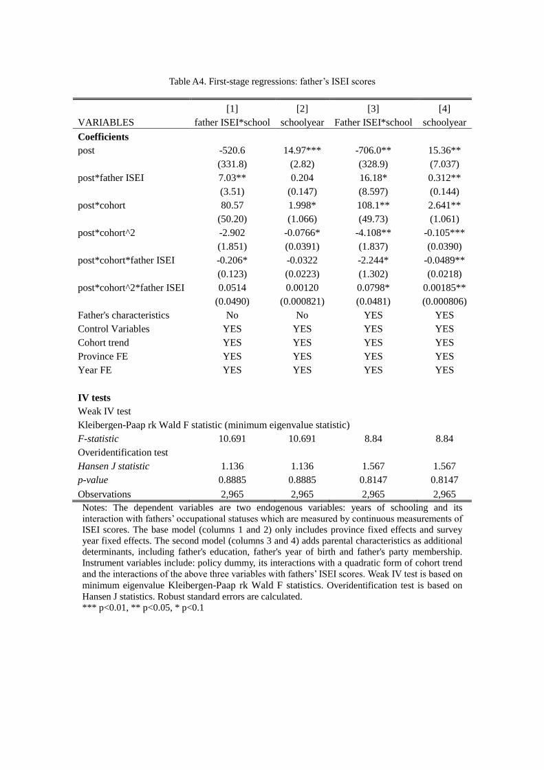
Table A4. First-stage regressions: father’s ISEI scores

[1] [2] [3] [4]

VARIABLES father ISEI*school schoolyear Father ISEI*school schoolyear

Coefficients

post -520.6 14.97*** -706.0** 15.36**

(331.8) (2.82) (328.9) (7.037)

post*father ISEI 7.03** 0.204 16.18* 0.312**

(3.51) (0.147) (8.597) (0.144)

post*cohort 80.57 1.998* 108.1** 2.641**

(50.20) (1.066) (49.73) (1.061)

post*cohort^2 -2.902 -0.0766* -4.108** -0.105***

(1.851) (0.0391) (1.837) (0.0390)

post*cohort*father ISEI -0.206* -0.0322 -2.244* -0.0489**

(0.123) (0.0223) (1.302) (0.0218)

post*cohort^2*father ISEI 0.0514 0.00120 0.0798* 0.00185**

(0.0490) (0.000821) (0.0481) (0.000806)

Father's characteristics No No YES YES

Control Variables YES YES YES YES

Cohort trend YES YES YES YES

Province FE YES YES YES YES

Year FE YES YES YES YES

IV tests

Weak IV test

Kleibergen-Paap rk Wald F statistic (minimum eigenvalue statistic)

F-statistic 10.691 10.691 8.84 8.84

Overidentification test

Hansen J statistic 1.136 1.136 1.567 1.567

p-value 0.8885 0.8885 0.8147 0.8147

Observations 2,965 2,965 2,965 2,965

Notes: The dependent variables are two endogenous variables: years of schooling and its

interaction with fathers’ occupational statuses which are measured by continuous measurements of

ISEI scores. The base model (columns 1 and 2) only includes province fixed effects and survey

year fixed effects. The second model (columns 3 and 4) adds parental characteristics as additional

determinants, including father's education, father's year of birth and father's party membership.

Instrument variables include: policy dummy, its interactions with a quadratic form of cohort trend

and the interactions of the above three variables with fathers’ ISEI scores. Weak IV test is based on

minimum eigenvalue Kleibergen-Paap rk Wald F statistics. Overidentification test is based on

Hansen J statistics. Robust standard errors are calculated.

*** p<0.01, ** p<0.05, * p<0.1

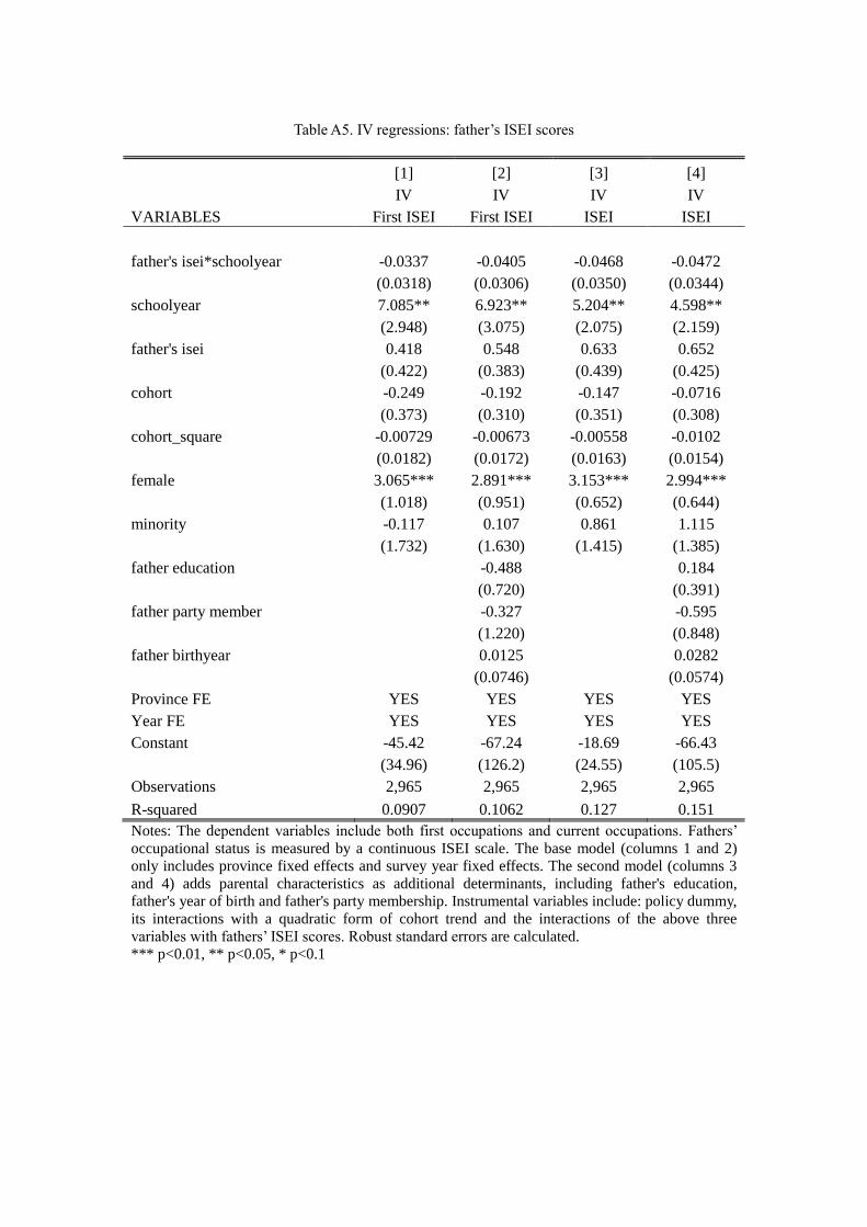
Table A5. IV regressions: father’s ISEI scores

[1] [2] [3] [4]

IV IV IV IV

VARIABLES First ISEI First ISEI ISEI ISEI

father's isei*schoolyear -0.0337 -0.0405 -0.0468 -0.0472

(0.0318) (0.0306) (0.0350) (0.0344)

schoolyear 7.085** 6.923** 5.204** 4.598**

(2.948) (3.075) (2.075) (2.159)

father's isei 0.418 0.548 0.633 0.652

(0.422) (0.383) (0.439) (0.425)

cohort -0.249 -0.192 -0.147 -0.0716

(0.373) (0.310) (0.351) (0.308)

cohort_square -0.00729 -0.00673 -0.00558 -0.0102

(0.0182) (0.0172) (0.0163) (0.0154)

female 3.065*** 2.891*** 3.153*** 2.994***

(1.018) (0.951) (0.652) (0.644)

minority -0.117 0.107 0.861 1.115

(1.732) (1.630) (1.415) (1.385)

father education

-0.488

0.184

(0.720)

(0.391)

father party member

-0.327

-0.595

(1.220)

(0.848)

father birthyear

0.0125

0.0282

(0.0746)

(0.0574)

Province FE YES YES YES YES

Year FE YES YES YES YES

Constant -45.42 -67.24 -18.69 -66.43

(34.96) (126.2) (24.55) (105.5)

Observations 2,965 2,965 2,965 2,965

R-squared 0.0907 0.1062 0.127 0.151

Notes: The dependent variables include both first occupations and current occupations. Fathers’

occupational status is measured by a continuous ISEI scale. The base model (columns 1 and 2)

only includes province fixed effects and survey year fixed effects. The second model (columns 3

and 4) adds parental characteristics as additional determinants, including father's education,

father's year of birth and father's party membership. Instrumental variables include: policy dummy,

its interactions with a quadratic form of cohort trend and the interactions of the above three

variables with fathers’ ISEI scores. Robust standard errors are calculated.

*** p<0.01, ** p<0.05, * p<0.1

Table A6. First-stage regression with household fixed effect

[1] [2] [3]

Probit Probit Probit

VARIABLES upper middle down

reform*cohort 0.533*** 0.175 0.251**

(0.203) (0.182) (0.115)

reform*cohort_square -0.000269*** -8.85e-05 -0.000127**

(0.000102) (9.19e-05) (5.80e-05)

age -0.388 -0.468 -0.632***

(0.367) (0.375) (0.210)

age_square 0.00397 0.00474 0.00694**

(0.00482) (0.00492) (0.00276)

female -0.181 -0.466** -0.698***

(0.173) (0.186) (0.103)

Constant 21.48*** 23.40*** 25.47***

(6.929) (7.070) (3.943)

Observations 134 131 437

Notes: First-stage regressions of Probit models with household fixed effect. Standard errors are in

parentheses. Columns 1, 2 and 3 refer to individuals from upper-class, middle-class and

working-class families. Instrumental variables are not valid for middle-class children. Standard

errors are clustered at the provincial level. Data source: RUMiC 2008.

*** p<0.01, ** p<0.05, * p<0.1