higher education reform cops working paper 16 march 2015

Centre of Policy Studies Working Paper

No. G-252 March 2015

Alternative Approaches to Fee Flexibility: Towards a

Third Way in Higher Education Reform in Australia

P. J. Dawkins and J.M. Dixon1

Victoria University

ISSN 1 031 9034 ISBN 978-1-921654-60-2

The Centre of Policy Studies (CoPS), incorporating the IMPACT project, is a research centreat Victoria University devoted to quantitative analysis of issues relevant to economic policy.Address: Centre of Policy Studies, Victoria University, PO Box 14428, Melbourne, Victoria, 8001home page: www.vu.edu.au/CoPS/ email: [email protected] Telephone +61 3 9919 1877

1 We are grateful to the Australian Government Department of Education and Training for providing

data on which this paper is based, and to comments and suggestions provided by Peter Noonan and

Alan Farley. We have also benefitted from discussions with Bruce Chapman and the opportunity to

present an overview of the ideas in this paper to the Senate Committee on Education and Employment

in their March 2015 inquiry into the higher education and research reform bill. The paper has also

benefitted from discussions with a number of people at the 2015 UA Conference, especially with Glyn

Davis.

Abstract

A major issue for the future of tertiary education is to ensure that Australia continues to expand its

investment in skills and capabilities, to enable a future of prosperity which is available to all. This has

been the aim of the demand‐driven system of higher education. The Federal Government’s current

proposals for higher education reform include the expansion of the demand‐driven system, by

bringing sub‐degree higher education programs into the subsided system and by bringing non‐

university higher education providers into the system.

At the same time the government has been seeking to achieve budget restraint and as a result

proposed to cut the amount of funding per student by an average of 20 per cent, although there is

considerable variation across the disciplines. The government has also proposed to uncap fees, so

that universities could at least recoup the lost funds due to the cuts in subsidies.

The government’s proposal for full‐fee deregulation in higher education has stalled in the Senate. It

has been subjected to criticism from the cross‐benchers and from a number of expert commentators

that there are serious risks with the proposal including the risk of excessive student fees and

excessive debts.

We argue that what is required is not full deregulation of fees, or a return to a more regulated

model with tight fee regulation and a possible reversion to more regulation of student numbers as

well. What is required is a ‘third way’ incorporating some degree of price flexibility, and an enhanced

equity package, while retaining the demand driven model.

This paper, therefore, is concerned with exploring alternative ways of sustaining the demand driven

system by allowing some degree of flexibility in student fees, while avoiding excessive fee rises and

allowing for some degree of price competition. Consideration is also given to ways in which the

equity aspects of the package could be enhanced.

Dawkins (2014) argued that three alternative methods should be explored to achieve a degree of fee

flexibility: fee caps, loan caps and a “taper model” whereby government tuition subsidies are

reduced according to a taper‐rate schedule, when they raise fees above a threshold level. The latter

concept is one that is also being proposed by Bruce Chapman (Chapman 2015).

Our analysis and consideration of the policy challenge leads us to the conclusion that the most

promising way forward is a two‐part package incorporating

i. a taper model whereby tuition subsidies are reduced according a progressive taper rate

schedule, when fees rise above a threshold level

ii. an enhanced Higher Education Participation Program (HEPP), incorporating scholarships for

all low socioeconomic status background students across the system, and additional

support for interventions for reducing the attrition rates of at‐risk students.

Data has been provided by the Commonwealth Department of Education and Training to assist with

this research and the modelling has been undertaken at the Centre of Policy Studies at Victoria

University.

1

1. Introduction

Over the last thirty years there has been a sequence of reforms to higher education (See Noonan

2015, for an overview).

The “Dawkins Revolution” in the 1980s involved a major expansion of higher education with a

number of former Colleges of Advanced Education and Institutes of Technology becoming

Universities. It was accompanied by the Introduction of the Higher Education Contribution Scheme

(HECS) which introduced fees for undergraduate education accompanied by income contingent

loans. In the early 2000s, when Brendan Nelson was the Minister for Education, the caps on the

HECS fees were lifted.

Thus, the last three decades has seen the size of the higher education system expand considerably.

Students first started to pay a contribution to their tuition costs and later the fees were increased.

These fees and their rise were justified on efficiency and equity grounds on the basis that students

received a substantial return on their investment, and as the system expanded students would need

to pay a higher share of the costs.

Following the Bradley Review (Bradley et al 2008), during the period of the Rudd‐Gillard

Government, the demand‐driven system was introduced which uncapped the number of bachelor

degree places that universities could offer, which provided for a further expansion of the system.

All of this expansion was driven by the case for expanding the size of the skilled workforce and the

need for an increasing number of graduates to enable ongoing technological change and

productivity growth.

While there was an uncapping of the number of subsidised places in universities under the reforms

following the Bradley Review, fees remained regulated, with fee caps in place. All universities charge

at the caps. Thus we have had a deregulation of quantities but not prices.

After the election of the Abbott Government, the new Minister, Christopher Pyne, asked David

Kemp and Andrew Norton to conduct a review (Kemp and Norton, 2014), of the demand driven

model. They concluded that it was a good idea and needed to be expanded by uncapping sub‐degree

higher education programs and bring non university higher education providers into the subsidised

system.

Then in the 2014 Budget, the Government announced that it would expand the demand driven

system in this way, but due to this expansion and to the need for budget restraint, government

subsidies to higher education students would be cut by 20 per cent. To enable providers to make up

for these cuts and to allow them to compete on price, fees for undergraduate courses would be fully

deregulated. Thus the fee caps would be removed. The caps on loans would also be removed.

This has resulted in a major debate about whether this fee deregulation is in the public interest. A

number of commentators, including one of the current authors, have argued that the policy setting

bring with them serious risks (Dawkins 2014).

2

The government has also not found it possible to get their legislation through the Senate, with a

number of the cross‐benchers concerned especially about the deregulation of fees and its potential

impact on students.

If there is no increase in student contributions, however, there are questions about whether, in a

period in where it is increasingly widely agreed that that expenditure restraint is necessary to

contain the budget deficit, the demand‐driven system and especially its expansion is able to be

continued.

This paper, therefore, is concerned with exploring alternative ways of sustaining the demand driven

system by allowing some degree of flexibility in student fees, while avoiding excessive fee rises and

allowing for some degree of price competition. Consideration is also given to ways in which the

equity aspects of the package could be enhanced.

Dawkins (2014) argued that three alternative methods should be explored to achieve a degree of fee

flexibility: fee caps, loan caps and a “taper model” whereby government tuition subsidies are

reduced according to a taper‐rate schedule, when they raise fees above a threshold level. The latter

concept is one that is also being proposed by Bruce Chapman (Chapman 2015).

These three options are explored in this paper.

Our analysis and consideration of the policy challenge leads us to the conclusion that the most

promising way forward is a two‐part package incorporating

iii. a taper model whereby tuition subsidies are reduced according a progressive taper rate

schedule, when fees rise above a threshold level

iv. an enhanced Higher Education Participation Program (HEPP), incorporating scholarships for

all low socioeconomic status background students across the system, and additional

support for interventions for reducing the attrition rates of at‐risk students.

Data has been provided by the Australian Government Department of Education and Training to

assist with this research and the modelling has been undertaken at the Centre of Policy Studies at

Victoria University.

2. The Government’s Current Proposals for Deregulation of Fees

In 2015, there will be more than 500,000 Equivalent Full Time (EFT) Commonwealth Supported

Places (CSPs) in Australian universities. Under the current system of funding, almost $6 billion, or

57% of total resourcing for CSPs, will be derived from the Australian Government Contribution, with

the remaining 43% provided by the student contribution.

As described above, to accommodate the expansion of the subsidised system to sub‐degree

programs and non‐university higher education providers and as part of a broader agenda of budget

restraint, the government aims to reduce its contribution to existing programs by 20% (equivalent to

11.4% of total resourcing for CSPs). In its simplest incarnation, this saving could be achieved by

reducing the Australian Government Contribution per student across all clusters by a uniform 20 per

3

cent. The shortfall in total resourcing to the universities could be made up by increasing maximum

student contributions by 26.5% (=11.4/43) across all clusters.

However, the current round of higher education reform includes other proposals.

Firstly, the government proposes to realign commonwealth support across the clusters by instead

allocating the disciplines into five funding tiers based on “private benefits for graduates, the

standard teaching method and infrastructure required to deliver the course.”1 Support will be

calibrated to achieve a saving of 20%.2

Secondly, the government proposes to deliver more decision‐making power to the universities by

deregulating prices. This would enable the universities to use student contributions to not only

make up the shortfall in total resourcing, but also to increase total resourcing. Noonan (2015) and

Chapman (2015), among others, identify the many risks associated with full fee deregulation. There

is a real risk of very high fee increases in an environment where the relationship between price and

demand, significantly negative for most commodities, is muddied by

Low interest income contingent loans removing the immediacy of price considerations in

the decision to purchase; and

The perception of price as a quality indicator, leading to the Veblen effect (Chapman

(2015).

In Figure 1, we show what could happen when the government cuts subsidy payments by 20 per

cent as in their current proposals. We assume that Go8 universities increase student contributions

by 100 per cent. A uniform increase in the student contribution charged by non‐Go8 universities is

illustrated on the horizontal axis, and the net percentage increase in university revenue (including

student contribution and government contribution) is shown on the vertical axis. Six scenarios for

the aggregate elasticity of demand (e) are shown3. In theory, as prices increase, demand falls and

this eventually has a negative impact on revenue. As illustrated in the chart, this effect becomes

more obvious the higher is the elasticity of demand. However, even with e=0.15 (a fairly high

estimate for the elasticity of demand) revenue is still growing with price increases in excess of 100%.

Only with a very high elasticity (e=0.25) does revenue growth start to drop away with price increases

in excess of 30%.

The elasticity of demand for education has been estimated by DAE (2011) using data on the

response of aggregate enrolments to increases in HECS. They find that “a 1% increase in the average

overall price of higher education corresponds to a 0.026 percentage point decrease in total

commencements.” In the medium term (by the time the change in commencements has worked

through the system, i.e. three years for an ordinary degree) we assume that this is equivalent to a

1 Department of Education (https://education.gov.au/public‐universities) 2 Davis and Dawkins (2014) and Dawkins (2014) have argued that the underpinnings of cluster funding rates require a thorough review. 3 The aggregate elasticity of demand is assumed to be a weighted average of the Go8 elasticity (assumed to be zero or very close to zero) and the non‐Go8 elasticity. In practice this means that the elasticity of demand for non‐Go8 universities is equal to the aggregate elasticity divided by 0.68 (the share of students at non‐Go8 universities). In practice the Go8 result could be inferred from the case where e=0, and the result for other universities from one of the cases where e>0. We assume a linear demand curve, so that the magnitude of the elasticity increases as price increases and quantity falls.

4

decrease in all enrolments of 0.026%. That is, the DAE estimate of the aggregate demand elasticity

for university education is 0.026. In this case, even with prices increased by 120 per cent as shown

in Figure 1, growth in revenue shows little sign of slowing down.

If universities do not implement large increases in price under deregulation, it may be because

‐ The elasticity of demand is higher (perhaps ten times higher) than that estimated by DAE;

‐ Universities are not acting to maximise revenue, possibly because of

o Universities’ concern for their public reputation or their view about what is in the

public interest;

o the prospect of competition from new entrants to the sector; or

o The prices are an opening gambit and could rise much further in the future.

If it is true that the elasticity of demand is high enough to act as an effective barrier to excessive

increases in price, then we must also consider the consequences of reduced enrolments on national

welfare, particularly in the long run. For example, if the aggregate elasticity of demand is 0.25, then

non‐Go8 universities will maximise revenue with a price increase of around 35 per cent, and

enrolments at these universities will fall by 13 per cent. This is equivalent to a fall in aggregate

enrolments of 9 per cent (assuming enrolments at Go8 universities are unaffected). In the long run,

this risks de‐skilling of the workforce, with obvious consequences for productivity and national

welfare In this case, aggregate revenue at the non‐Go8 universities will also fall (by 10 per cent),

although revenue per student will increase. Under this scenario it is possible that non‐university

higher education providers might fill the gap.

Figure 1: University revenue under full deregulation with 20% cut in subsidy, for several values of the aggregate elasticity of demand for higher education

‐10.00%

‐5.00%

0.00%

5.00%

10.00%

15.00%

20.00%

25.00%

30.00%

35.00%

40.00%

0 6

12

18

24

30

36

42

48

54

60

66

72

78

84

90

96

102

108

114

120Chan

ge in

total university revenue (%)

Uniform increase in non‐Go8 student contribution (%)

e=0

e=0.025

e=0.05

e=0.1

e=0.15

e=0.25

5

A deregulated system therefore carries the risk of either high price increases or risks significant falls

in enrolments, both with undesirable impacts on national welfare. As Chapman has outlined

(Chapman 2015), there are strong reasons to believe that demand elasticity is low (which prevents a

large drop in enrolments). The existence of low‐interest income‐ contingent loans, with a repayment

system that results in price increases resulting in no increase in repayments until payments are

completed to pay‐off the base price, is a major factor in keeping price sensitivity very low.

An optimistic scenario is that universities, motivated by concerns other than revenue‐maximising,

will not implement large increases in prices. While competition between providers may moderate

prices to some extent, Chapman (2015) argues that it is unlikely to have much effect. Thus under full

fee deregulation, the community has to trust the universities not to engage in significant price hikes.

3. Alternatives to deregulation

3.1. Alternative 1: A Fee Cap

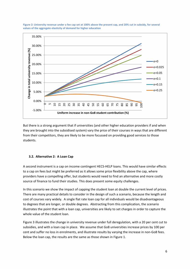
Experience and our modelling suggest that unless these caps are set very high, every university will

move to the cap. Figure 2 illustrates a fee cap set at 100 per cent above current prices. Again we

assume that the Go8 universities will increase prices by 100 per cent (that is, they will charge at the

cap) and suffer no loss in enrolments. Possible price increases by the non‐Go8 universities are

shown on the horizontal axis. If the elasticity of demand is sufficiently high, revenue growth slows

down as the non‐Go8 fees increase. However, at a fee cap of 100 per cent, non‐Go8 universities will

still maximise revenue by charging at the fee cap, for a realistic range of elasticities.

If the fee cap was higher, it is possible that not all universities would charge at the fee cap.

However, a fee cap of more than 100 per cent above the existing cap would not be an effective

means addressing the problems with deregulation, such as equity concerns or large bad debts

through the HECS system.

6

Figure 2: University revenue under a fee cap set at 100% above the present cap, and 20% cut in subsidy, for several values of the aggregate elasticity of demand for higher education

But there is a strong argument that if universities (and other higher education providers if and when

they are brought into the subsidised system) vary the price of their courses in ways that are different

from their competitors, they are likely to be more focussed on providing good services to those

students.

3.2. Alternative 2: A Loan Cap

A second instrument is a cap on income contingent HECS‐HELP loans. This would have similar effects

to a cap on fees but might be preferred as it allows some price flexibility above the cap, where

providers have a compelling offer, but students would need to find an alternative and more costly

source of finance to fund their studies. This does present some equity challenges.

In this scenario we show the impact of capping the student loan at double the current level of prices.

There are many practical details to consider in the design of such a scenario, because the length and

cost of courses vary widely. A single flat rate loan cap for all individuals would be disadvantageous

to degrees that are longer, or double degrees. Abstracting from this complication, the scenario

illustrates the point that with a loan cap, universities are likely to set charges in order to capture the

whole value of the student loan.

Figure 3 illustrates the change in university revenue under full deregulation, with a 20 per cent cut to

subsidies, and with a loan cap in place. We assume that Go8 universities increase prices by 100 per

cent and suffer no loss in enrolments, and illustrate results by varying the increase in non‐Go8 fees.

Below the loan cap, the results are the same as those shown in Figure 1.

‐5.00%

0.00%

5.00%

10.00%

15.00%

20.00%

25.00%

30.00%

35.00%

0 5

10

15

20

25

30

35

40

45

50

55

60

65

70

75

80

85

90

95

100

Chan

ge in



e=0

e=0.025

e=0.05

e=0.1

e=0.15

e=0.25

7

Above the loan cap, we assume that demand falls away very quickly, as students must find an

alternative source of funds. We assume that for every 1 per cent increase in price above the loan

cap, demand falls by 1 per cent. That it may fall by more does not change the central argument,

which is that the revenue‐maximising strategy of universities will be to charge the full loan cap.

A key problem with the loan cap is that it will not achieve any price diversity in the sector as all

providers are likely to price at the value of the loan cap.

Figure 3: University revenue under a loan cap set at 100% above the current fee cap, and 20% cut in subsidy

3.3. Alternative 3 Tapering Government Subsidies when Fees Rise

3.3.1. The concept

A third option is to vary the government's subsidy to providers depending on the prices that they

charge. Those providers charging the highest prices would receive lowest subsidies. This idea was

floated as a possible option by Dawkins (2014) and in his submission to the Senate inquiry in the

Higher education Reform, Chapman (2015) argues strongly that an approach of this kind is the way

forward.

Chapman writes

‐15.00%

‐10.00%

‐5.00%

0.00%

5.00%

10.00%

15.00%

20.00%

25.00%

30.00%

35.00%

0 6

12

18

24

30

36

42

48

54

60

66

72

78

84

90

96

102

108

114

120

Chan

ge in



e=0

e=0.025

e=0.1

e=0.15

e=0.2

e=0.25

8

“…a principal role of government is to design and enforce arrangements that encourage activities

that provide social benefits beyond the consequences of the private benefits to citizens”. (Chapman

2015 p.5)

He goes on to say

“..there are examples of public sector activity in which governments withhold and/or reduce

subsidies to citizens and institutions if their situations or behaviour warrant diminished support”

There are a number of key design issues in implementing the proposal. Our preferred option is

based on two key components:

A taper model whereby tuition subsidies are reduced according to a progressive taper rate

schedule as fees rise above threshold levels; and

An enhanced Higher Education Participation Program (HEPP), incorporating scholarships for all

low socioeconomic status background students across the system, and additional support for

interventions to reducing attrition rates for at‐risk students, in the expanded system

The details of the proposal are, of course, very amenable to variation, and are put up as a starting

point for a discussion about what the desirable properties of such a plan should be. Chapman’s

proposal is very similar and we give some analysis of it in Appendix 3.

3.3.2. The Dawkins‐Dixon taper scheme

The current version of the Dawkins‐Dixon plan reduces the cut in the government subsidy rate from

20 per cent to 5 per cent. It is our view that to undertake a cut of 20 per cent alongside a very

significant reform program would place undue strain on the system. It would of course, be open to

government not to reduce the subsidy at all.

The chosen threshold fee, at which the first taper is introduced, is set at a level where total funding

per student, including the adjusted subsidy, would be 10 per cent higher than at present. This is

based on the fact that two government reviews in recent years, Bradley (2008) and Lomax‐Smith

(2011), concluded that funding per student needed to rise by 10 per cent to adequately provide for

the level of quality of teaching and learning on which we should not be willing to economise.

At the first threshold, the taper rate is 20 per cent. This is progressively increased in steps of 10

percentage points up to a maximum of 90 per cent at approximately twice the current prices.

Figure 4 below illustrates how the taper scheme might work, using Humanities as an example.

Under the present system, Humanities students pay $6,152 in fees, with the government

contributing a further $5,447, for total resourcing of $11,599. Humanities does relatively well in the

government’s proposed re‐estimation of subsidies. Even after the government’s proposed 20 per

cent cut to aggregate subsidies, the subsidy to Humanities is barely touched, coming in at $5,332 per

full‐time equivalent student. With the lesser cut averaging just 5 per cent, government support for

Humanities places actually increases.

9

The full set of subsidy changes is given in Appendix 1. This, of course, is another design feature that

can be the subject to further discussion, if the basic principles of this policy design are accepted.

In Figure 4 we illustrate how the subsidy would be tapered downwards if the student contribution is

increased in the area of Humanities. Under the taper scheme, as the student contribution increases,

the subsidy is gradually tapered away. At a sufficiently high price, growth in total funding per

student eventually grinds to a halt. This is to curb any tendency in the universities towards excessive

price increases.

The green line in Figure 4 illustrates the government’s proposal for a 20 per cent cut to aggregate

subsidies and deregulated fees. With prices close to their present level, the taper scheme returns

more revenue to the universities because it embodies only a 5 per cent cut to aggregate subsidies.

However, as prices climb in the fully deregulated version, universities are not penalised. We are left

without an explicit safeguard against excessive price increases.

The full set of taper rates and thresholds is shown in Appendix 1.

Figure 4: The Taper Scheme for Humanities

3.3.3. A possible scenario

In choosing a scenario with which to illustrate the Dawkins‐Dixon taper scheme, we generated a

series of results for university revenue under different assumptions about increases in fees and

demand elasticities. These are shown in Appendix 2. The following analysis relates to a scenario

that we consider a good illustration of the likely pricing decisions by universities.

Group of Eight universities

$‐

$2,000

$4,000

$6,000

$8,000

$10,000

$12,000

$14,000

$16,000

$18,000

$20,000

$6152(2015

settings)

$6,000 $7,000 $8,000 $9,000 $10,000 $11,000 $12,000 $13,000

Total funding per student

Student contribution

Student Contribution Government Contribution Deregulated total, 20% subsidy cut

10

Our analysis leads us to the indicative conclusion that the Group of Eight (Go8) universities would be

likely to decide to charge their various courses at the tops of either the 50 per cent, 60 per cent, 70

per cent or 80 per cent taper thresholds, and that they would not need to experience a drop in

enrolments as a result. With students accessing income contingent loans at a real interest rate of

zero, our indicative assessment is that the net present value of typical4 student’s contribution for a

year’s tuition would increase by an average of about $3000. This is substantially lower than the kind

of rises that have been mooted under the fully deregulated model.

As an illustration, if all of the Go8 universities charged at the top of the 60 per cent taper, the

government contribution to the Go8 universities falls to $1.7 billion in 2016.5 Compared to the

business‐as‐usual case – the present system applied to 2016, with some natural growth in student

numbers and inflation – this is a saving of $400 million. With the increase in fees, the Go8

universities’ revenue increases to $4.3 billion in aggregate in 2016, or 18 per cent compared to

business as usual.

Other universities

It is quite possible that some or all of the 31 non‐Go8 universities will experience a drop in

enrolments if they engage in large fee increases. Our analysis leads us to the indicative conclusion

that these universities will charge less than the Go8, possibly pricing at the tops of either the 20 per

cent, 30 per cent, 40 per cent or 50 per cent taper thresholds.

As an illustration, if all of the non‐Go8 universities charged at the top of the 30 per cent taper, the

net present value of student contributions for a year’s tuition for a typical6 student would increase

by about $2,000. We estimate that there could be a fall in enrolments in non‐Go8 universities of

around 2.5 per cent. These students might instead go to non‐university higher education providers,

or a vocational education course.

We estimate that the government’s contribution to non‐Go8 universities would fall to about $3.8

billion, a saving of $400 million compared to business as usual. The revenue of the universities

would grow to $8.2 billion, an increase of 12 per cent compared to business‐as‐usual, and in line

with the Bradley/Lomax Smith recommendations.

The total government contribution to the universities is therefore $5.5 billion, a total saving of $800

million compared to business as usual.

4 For example, for a student who would have taken ten years to discharge her HECS debt at the current fees, the fee increase will be paid in the eleventh year and beyond. If the face value of the fee increase is, for example, $5600, but it is not required until 11 or 12 years’ time, the net present value of the fee increase is significantly lower at around $3000. For the many students who take longer than this to discharge their HECS debts, the net present value of the same fee increase would be much lower. Furthermore, as the HECS system is designed to insure students against the risk of default or repayment hardship, this estimate is likely to be an overstatement of the value of the fee increase for most students. 5 We simplify the analysis by assuming that all students in 2016 will be subject to the new subsidy rates. In practice, those who commenced prior to the 2014 budget will still fall under the old subsidy rates. 6 A student who would have taken ten years to discharge his HECS debt at the current fees.

11

Figure 5: Sources of University funding in 2016, Business as usual (2015 policy settings) and Taper scheme

3.3.4. The enhanced HEPP program

We propose that at least a proportion of the savings to government should be used to finance a

stronger equity package to include a system‐wide scholarship fund for all students from low socio‐

economic backgrounds. Some of the funds could also be used for interventions to reducing attrition

rates for at‐risk students, in the expanded system.

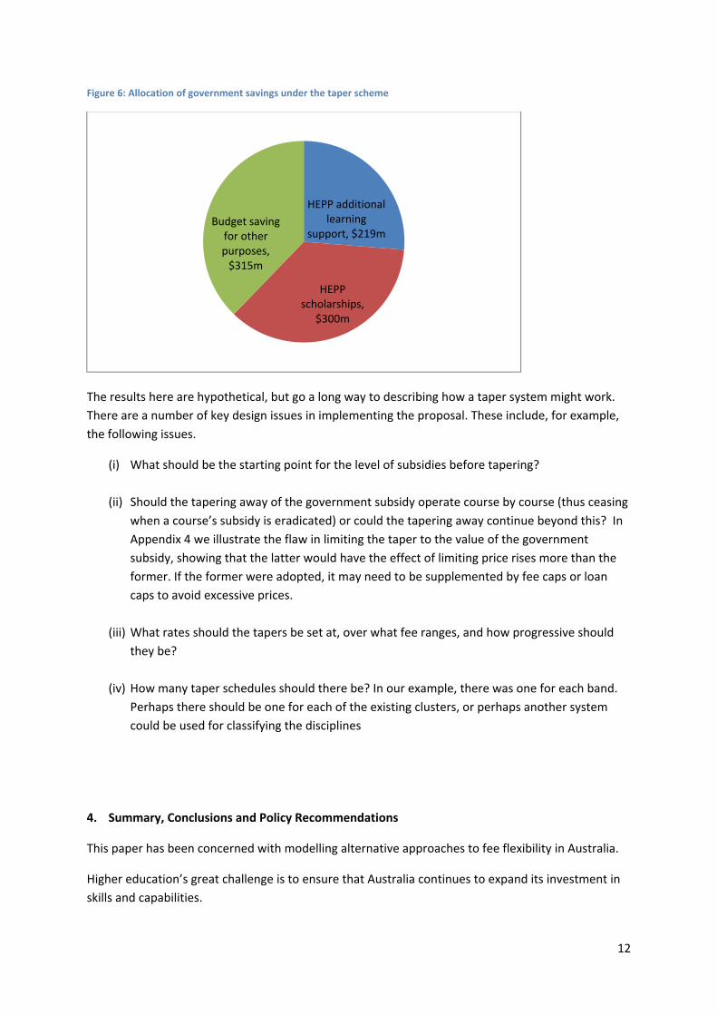
A possible allocation for the saving in our example above would be:

$300 million to be allocated to HEPP scholarships for students from low socio economic

status backgrounds. There are presently approximately 150,000 low‐SES students, so this

fund would be sufficient to pay each individual a scholarship of $2000.

$315 million, equivalent to the saving from the 5 per cent subsidy reduction, which could be

used for general budget savings or other purposes. In part this might help take the pressure

away from the possibility of cuts to research budgets. It might also help with the

implementation of a structural adjustment package for those universities that are most

challenged by this kind of reform agenda.

The remaining funds (approximately $219 million) to be used to support intervention

programs through the HEPP program for low SES students and others identified to be at risk

of discontinuing their studies.

0

1000

2000

3000

4000

5000

Government contribution:Go8 ($m)

Student contribution(supported by interestfree, income contingent

loan): Go8 ($m)

Government contribution:non‐Go8 ($m)

Student contribution(supported by interestfree, income contingentloan): non‐Go8 ($m)

Business as usual

Taper scheme

12

Figure 6: Allocation of government savings under the taper scheme

The results here are hypothetical, but go a long way to describing how a taper system might work.

There are a number of key design issues in implementing the proposal. These include, for example,

the following issues.

(i) What should be the starting point for the level of subsidies before tapering?

(ii) Should the tapering away of the government subsidy operate course by course (thus ceasing

when a course’s subsidy is eradicated) or could the tapering away continue beyond this? In

Appendix 4 we illustrate the flaw in limiting the taper to the value of the government

subsidy, showing that the latter would have the effect of limiting price rises more than the

former. If the former were adopted, it may need to be supplemented by fee caps or loan

caps to avoid excessive prices.

(iii) What rates should the tapers be set at, over what fee ranges, and how progressive should

they be?

(iv) How many taper schedules should there be? In our example, there was one for each band.

Perhaps there should be one for each of the existing clusters, or perhaps another system

could be used for classifying the disciplines

4. Summary, Conclusions and Policy Recommendations

This paper has been concerned with modelling alternative approaches to fee flexibility in Australia.

Higher education’s great challenge is to ensure that Australia continues to expand its investment in

skills and capabilities.

HEPP additional learning

support, $219m

HEPP scholarships,

$300m

Budget saving for other purposes, $315m

13

There is very little sign that government budgets are going to provide the long‐term solution to

support the growing resource needs of an expanding system that also aspires to excellence. It seems

inevitable that in an increasingly large tertiary system, students will be contributing more to the cost

of their education in the future. How do we achieve this without imposing too large a burden on

students and having seriously negative impacts on equity, while ensuring that students get an

enhanced education?

Income contingent loans will continue to be a key. However, as is evident from our modelling, fully

deregulated fees do not provide an efficient or equitable solution to the need for larger student

contributions. There is a genuine risk that under full fee deregulation, universities, in the long run

will act to maximise revenue and over time implement very large increases in prices, above the

socially optimum level.

The equity strategy in the current plan is to create Commonwealth scholarship funds which will be

largest in those universities charging the highest fees. While this may look reasonable to some at

first sight, these would likely be the universities with the fewest students from lower socio‐economic

backgrounds, both before and after the disbursement of scholarships. It is in the national interest to

create a whole‐of‐system scholarship fund that is equally supportive of students from poorer

backgrounds wherever they study. Universities charging the highest fees could, of course, top up

these scholarships as part of their own equity strategies.

What is needed is a redesigned approach to allow for increased but not excessive student

contributions, that enables an increase in the quality and quantity of tertiary education and

promotes access and success for students from lower socioeconomic backgrounds.

One of three possible policy instruments could be used to allow for increased but not excessive

student contributions.

The first is to raise the cap on fees. Experience and our modelling suggest that unless these caps are

set very high, every university will move to the cap. But there is a strong argument that universities

and other higher education providers, varying the price of their courses in ways that are different

from their competitors, are likely to be more focussed on providing good services to those students.

A second instrument is to cap the loans. This would have similar effects to a cap on fees but might be

preferred as it allows some price flexibility above the cap, where providers have a compelling offer,

but students would need to find an alternative and more costly source of finance to fund their

studies. This presents some equity challenges.

A third way is to vary the government's subsidy to providers depending on the prices they charge.

Those providers charging the highest prices would receive the lowest subsidies. This idea is also

being proposed by Bruce Chapman and is consistent with basic principles of equity and efficiency in

public financing. Our modelling suggests that this is more likely to result in price competition but

could be designed in such a way as to avoid excessive price rises. At the upper limit, a one‐dollar rise

could result in a one‐dollar loss of subsidy, which is effectively a price cap. But if the taper for

subsidy withdrawal starts at a lower rate and is progressively increased, it would be likely to be more

effective in restraining prices. In practice we think that a 90 per cent taper would be the highest

needed in such a system.

14

This has the added advantage that government funding saved from the withdrawal of subsidies

could be used to fund system‐wide equity scholarships. Some of the funds could also be used for

interventions to reducing attrition rates for at‐risk students in the expanded system. Our paper

suggests that the most promising way forward in meeting this policy challenge is s two part

strategy:‐

(i) a taper system, with a design that would not require it to be supplemented with a

fee cap or a loan cap

(ii) an expanded equity and participation package using the funds saved from the

reduction in the subsidies when fees rise.

A particular design is presented, which the authors argue have desirable features and would have

desirable outcomes. As important, however, is that the policy design is flexible and very amenable to

amendment depending upon the weight placed on different objectives. It is hoped that this could

form the basis of a discussion – with the government, the Senate, the higher education sector and

the broader community – that could ultimately lead to suitable package along these lines.

15

Appendix 1: More details on the tapers thresholds etc. in the Dawkins‐Dixon preferred model.

The taper system

Universities may increase fees to increase revenue. Fee increases will result in a reduction of

subsides at an increasing taper rate (see Table 1) to act as deterrent to very high increases with

the maximum taper at 90 per cent. Relative to Chapman (2015), the number of bands of taper

rates is increased, with the aim of producing a greater degree of price competition.

Assuming that government still requires some savings from the policy, the starting point is that

the cut in subsidy rates is 5 per cent which is equivalent to a saving in 2016 of just over $300

million compared to if the 2015 subsidy rates are carried forward to 2016 (assuming growth in

student numbers of 5 per cent).

Universities can increase fees in order to increase net revenue by 10 per cent without incurring

any penalty.

Table 1: Taper thresholds and rates

Band* New Student Contribution Marginal Taper rate

band 1 $0 ‐ $7,999 0%

($6152) $8,000 ‐ $8,499 20%

$8,500 ‐ $8,999 $9,000 ‐ $9,499 $9,500 ‐ $10,499 $1,0500 ‐ $10,999 $11,000 ‐ $11,499

30% 40% 50% 60% 70%

$11,500‐11,999 $12,000 and over

80% 90%

band 2 $0 ‐ $10,999 0%

($8768) $11000 ‐ $11,999 20%

$12,000 ‐ $12,999 $13,000 ‐ $13,499 $13,500 ‐ $13,999

30% 40% 50%

$14,000‐ $14,999 $15,000‐ $15,999 $16,000‐ $16,999 $17,000 and over

60% 70% 80% 90%

band 3 $0 ‐ $12,999 0%

($10266) $13,000 ‐ $13,999 20%

$14,000 ‐ $14,999 30%

$15,000 –$ 15,999 $16,000‐ $16,999 $17,000‐$17,999 $18,000‐$18,999 $19,000‐$19,999 20,000 and over

40% 50% 60% 70% 80% 90%

* current student contribution in parentheses at 2015 prices

16

The structure of subsidies

The subsidies are calculated according to the Department of Education’s cost of delivery model,

which is designed to reflect the cost of delivery for each of five tiers. Each tier is allocated a cost

coefficient. The subsidies are then calculated in order to reflect the relative cost coefficients, and

calibrated to achieve the required budget saving.

For this modelling exercise, we adopted the same approach, with two variations. Firstly, we

adjusted the cost coefficient for Tier 1 (equivalent to Cluster 1) from 0.3 to 0.6, effectively doubling

the subsidy for this tier. Even with this adjustment, Tier 1 still receives the lowest subsidy. Secondly,

we calibrated the subsidies to achieve a real cut of 5 per cent to subsidy payments per EFT student.

Table 2 below show the subsidies calculated for 2016 compared to the existing 2015 subsidies. In

some cases, the 2015 clusters span more than one of the proposed five tiers, so the subsidy rate

shown is an average across the relevant tiers, weighted by EFT student numbers. The subsidy rate

for 2016 assumes indexation to inflation of 2.5 per cent.

Table 2

Cluster 2015 rate 2016 rate change

1 Law, accounting, commerce, economics, administration

$1961 $4089 108.5%

2 Humanities $5447 $6815 25.1%

3a Mathematics, statistics, computing, built environment or other health

$9637 $11452 18.8%

3b Behavioural science or social studies $9637 $8542 ‐11.4%

4 Education $10026 $10222 2.0%

5a Clinical psychology, foreign languages, or visual and performing arts

$11852 $9525 ‐19.6%

5b Allied health $11852 $12612 6.4%

6 Nursing $13232 $13630 3.0%

7 Engineering, science, surveying $16850 $13630 ‐19.1%

8a Dentistry, medicine or veterinary science $21385 $20445 ‐4.4%

8b Agriculture $21385 $20445 ‐4.4%

17

Appendix 2: Sensitivity analysis on the Dawkins Dixon preferred model

Figures 7, 8 and 9 below illustrate results for Bands 1, 2 and 3 respectively, for several values of the

elasticity of demand. What is clear from these charts is that (a) the taper system causes revenue‐

maximising points to fall within a reasonable range of price increases, and (b) that the pricing

strategies that will maximise revenue depend on both the taper schedule and the elasticity of

demand.

Revenue maximising fees for the various elasticity scenarios are shown in Table 3 below. The results

show that revenue maximising points tend to be at the threshold between one taper rate and the

next. This suggests that a system in which there are many taper rates will lead to greater diversity in

prices.

Universities will be motivated by concerns other than revenue maximising, such as preserving their

quality and reputation, and wanting to act in the national interest. For these reasons we believe a

scenario in which universities charge a fee that is somewhat below the revenue maximising fee is a

suitable example to use in illustrating the taper model.

Table 3: Results of sensitivity analysis

elasticity of demand (non‐Go8) Business‐as‐usual

0 0.025 0.05 0.1 0.15 0.25

Revenue‐maximising fee ($)

Band 1 n.a. n.a. 12000 11500 11000 9115 6306 Band 2 n.a. n.a. n.a. 16643 15260 13853 8987 Band 3 n.a. n.a. n.a. 20000 19001 18000 10523 Net Government contribution ($m)

Band 1 n.a. n.a. 1958 2000 2038 2271 2095 Band 2 n.a. n.a. n.a. 1863 2023 2130 1702 Band 3 n.a. n.a. n.a. 890 874 845 388

* the revenue maximising result is above the top taper threshold

In most but not all cases, the revenue maximising fees are at the boundary between two taper

thresholds.

Supposing that most Go8 universities have very low elasticity of demand, we hypothesise that the

revenue maximising fee for these universities is at or above the top taper threshold. The fee they

actually charge may be at the top of the 80 per cent threshold, or lower, perhaps at the tops of

either the 50 per cent, 60 per cent or 70 per cent thresholds.

The non‐Go8 universities may face higher elasticities, in the range of 0.05 to 0.15. In this case, the

revenue maximising fee may be at the tops of the 50 per cent, 60 per cent or 70 per cent thresholds.

The fee they actually charge may be lower, perhaps at the tops of the 20 per cent, 30 per cent, 40

per cent or 50 per cent thresholds.

18

Figure 7: University revenue, Band 1


‐10%

‐5%

0%

5%

10%

15%

20%

6307

6542

6777

7012

7247

7482

7717

7952

8187

8422

8657

8892

9127

9362

9597

9832

10067

10302

10537

10772

11007

11242

11477

11712

11947

Chan

ge in

university revenue (%)

Student Contribution ($)

e=0

e=0.025

e=0.05

e=0.1

e=0.15

e=0.25

‐10%

‐5%

0%

5%

10%

15%

20%

8988

9311

9634

9957

10280

10603

10926

11249

11572

11895

12218

12541

12864

13187

13510

13833

14156

14479

14802

15125

15448

15771

16094

16417

16740

Chan

ge in



e=0

e=0.025

e=0.05

e=0.1

e=0.15

e=0.25

19


0%

5%

10%

15%

20%

25%

30%

35%

40%

45%

50%

10524

10934

11344

11754

12164

12574

12984

13394

13804

14214

14624

15034

15444

15854

16264

16674

17084

17494

17904

18314

18724

19134

19544

19954

20364

Chan

ge in



e=0

e=0.025

e=0.05

e=0.1

e=0.15

e=0.25

20

Appendix 3: Chapman’s taper model

In his submission to the Senate Inquiry (Chapman 2015) as well as explaining and arguing for the

concept, Chapman outlined an example of how it could be implemented in terms of the bands and

tapers. This includes the following points

Universities may increase fees to increase revenue. Fee increases will result in a reduction

of subsides at an increasing taper rate (see Table 4) to act as deterrent to very high

increases.

The government would make budget savings through taper revenue.

The starting point for the subsidies (before tapering) is to completely reverse the 20 per cent

cut (retaining the 2015 subsidies plus inflation), but after the tapering the effective subsides

will be lower when providers choose to price above the first threshold at which the first

taper cuts in.

The first taper threshold has been chosen by Chapman to reflect the “projected (and

rounded) value of the current maximum student contribution in that band at 2016”.

Subsequent thresholds are set in $5000 steps.

Table 4

Band* New Student Contribution Marginal Taper rate

band 1 $0 ‐ $6,499 0%

($6152) $6,500 ‐ $11,499 20%

$11,500 ‐ $16,499 60%

$16,500 and over 80%

band 2 $0 ‐ $9,199 0%

($8768) $9,200 ‐ $14,199 20%

$14,200 ‐ $19,199 60%

$19,200 and over 80%

band 3 $0 ‐ $10,749 0%

($10266) $10,750 ‐ $15,749 20%

$15,750 ‐ $20,749 60%

$20,750 and over 80%

* current student contribution in parentheses at 2015 prices

Source: Chapman (2015)

Group of eight results

We assume that the Group of eight universities all decide to charge at the top taper threshold, and

that they suffer no drop in enrolments as a result. This amounts to an average fee increase per

student of 162% in Band 1, 114% in Band 2, and 97% in Band 3.

As a result of the subsidy cut and the taper, the government contribution to the Go8 universities falls

to $1.3 billion, a fall of $788 million compared to business as usual. With the increase in fees, the

21

Go8 universities’ revenue increases by $1.2 billion in aggregate, or 32 per cent compared to business

as usual.

Non‐Group of eight results

Results for the non‐Go8 universities are more difficult to forecast. It is not likely that these

universities could charge at the top taper threshold and suffer no drop in enrolments.

We present some illustrative results based on several possible scenarios for the elasticity of demand

in Figure 10 below, in which we show the impact of a uniform percentage increase in student

contributions across all clusters. Figure 10 shows that if the elasticity is less than about 0.05,

demand does not fall enough to have a negative impact on revenue, even at a price increase of

120%.

Chapman expects the Go8 universities would provide 55% of the reduction on grants savings, with

non‐Go8 providing the remaining 45%. We find that an example in which this is the case is when

Go8 universities implement a fee increase of 100% with no impact on enrolments, and non‐Go8

universities implement a fee increase of 70%, losing 2.5 per cent of enrolments (assuming an

elasticity of 0.035). In this case, the aggregate budget saving is $1.4 billion, a saving of 23 per cent

compared to business as usual.

Figure 10: Change in non‐Go8 university revenue under several scenarios for the aggregate elasticity of demand (e)

A number of points emerge from this design:‐

(i) The progressive rate structure does open up the possibility of restraining prices and may

result in some degree of price differentiation.

‐15.0%

‐10.0%

‐5.0%

0.0%

5.0%

10.0%

15.0%

20.0%

25.0%

30.0%

35.0%

0 5

10

15

20

25

30

35

40

45

50

55

60

65

70

75

80

85

90

95

100

105

110

115

120

Non‐Go8 increase in student contribution (%)

e=0

e=0.025

e=0.05

e=0.1

e=0.15

e=0.25

22

(ii) A top rate of 80 percent may not be high enough to provide an effective cap.

(iii) The amount of price competition will be affected partly by variations in the elasticity of

demand and partly by how many different taper rates apply. The modelling shows that

providers price choices can be expected to be at the top of the one of the taper bands.

The more taper bands there are the more likely it is that some price competition will

emerge.

(iv) In the example above, any budget savings arise from the tapering away of the subsidies.

In the government’s current proposals there is one taper, i.e. 20 per cent the revenue

from which the provider in question has use themselves for Commonwealth scholarships

to their own low socio‐economic background students. Dawkins (2014) has pointed out

that this means that scholarship funds will be largest in those universities charging the

highest fees. While this may look reasonable at first sight, this would likely be those

universities with the fewest students from lower socio‐economic backgrounds, both

before and after the disbursement of scholarships. He went on to argue that was in the

national interest to create a whole of system scholarship fund that is equally supportive

of students from poorer backgrounds wherever they study. Universities charging the

highest fees could, of course, top up these scholarships as part of their own equity

strategies.

Furthermore, the 20 per cent taper in the government’s proposal is for the scholarship

fund, and is not intended to provide budget savings.

(v) Another issue for the government if they still require budget savings from the plan, is

that the savings form this design are expected to be positive but are unknown. They

could be forecast on the basis of expected provider and student responses but could be

very inaccurate.

23

Appendix 4: Taper offset with subsidy

In this appendix we illustrate a potential flaw in the system if the taper remittances are offset

against subsidy payments. This is a problem if the subsidy is low enough to be tapered out while the

pricing is still below the maximum taper range.

For example, in Chapman’s model, in the case of Cluster 1, the student fees are only in the 60%

taper range when the subsidy is completely tapered out, creating the danger that universities will

have no disincentive preventing them from pricing above this range. Figure 11 shows revenue

growth for Cluster 1, for which the present student fee is around $10,000, slowing at a fee increase

of around $17,300. Under Chapman’s taper parameters, this is where taper payment reaches

approximately $2000 per student, which is the present subsidy for Cluster 1. Beyond this fee

increase, the taper system is no longer effective because the university suffers no penalty for

increasing student fees.

This flaw could be easily avoided, either by continuing to tax fee increases after the subsidy is

tapered out, or by setting the tapers so that the top taper threshold is below the original value of

the subsidy. Offsetting taper remittances against subsidies at the whole‐of‐university revenue may

also be an effective method of preventing this problem.

Because a high subsidy rate provides a large cushion against which to offset the taper payment, this

flaw is not apparent for the heavily subsidised clusters. Across the present cluster arrangement, the

subsidy rates vary from a low of 16% for Cluster 1 (Law, accounting etc.) to a high of 71% for part of

Cluster 8 (Agriculture).

Figure 11: Cluster 1 revenue to universities under Chapman's taper with taper remittances offset against subsidies

0.0%

10.0%

20.0%

30.0%

40.0%

50.0%

60.0%

70.0%

80.0%

90.0%

10523

11049

11575

12101

12627

13153

13679

14206

14732

15258

15784

16310

16836

17362

17889

18415

18941

19467

19993

20519

21045

21571

22098

22624

23150

Student contribution ($)

e=0

e=0.025

e=0.05

e=0.1

e=0.15

e=0.25

20% taperrange

60% taper range

24

References

Bradley, D., Noonan, P., Nugent, H., & Scales, B. (2008). Review of Australian Higher Education.

Commonwealth of Australia.

Chapman, B. (2015). A Submission to Senate Enquiry on Higher Education Reform.

Dawkins, P. (2014). Reconceptualising Tertiary Education and the case for re‐crafting aspects of the

Abbott Government's Proposed Higher Education Reforms. Mitchell Institute Policy Lecture,

22 May.

Deloitte Access Economics. (2011). The impact of changes to student contribution levels and

repayment thresholds on the demand for higher education.

Kemp, D., & Norton, A. (2014). Review of the Demand Driven Funding System. Commonwealth of

Australia.

Lomax‐Smith, J., Watson, L., & Webster, B. (2011). Higher Education Base Funding Review: Final

Report. Commonwealth of Australia.

Noonan, P. (2015). Building a sustainable funding model for higher education in Australia ‐ a way

forward. Mitchell Institute discussion paper.

Victoria University. (2015). Victoria University (VU) Submission to the Senate Education and

Employment Legislation Committee on the Higher Education and Research Reform

Amendment Bill 2014.

http://www.aph.gov.au/Parliamentary_Business/Committees/Senate/Education_and_Empl

oyment/Higher_Education_2/Submissions (Submission 35).

higher education reform cops working paper 16 march 2015

Documents