© Wenjie Ma, 2021

Higher-Point Conformal Blocks

Thèse

Wenjie Ma

Doctorat en physique

Philosophiæ doctor (Ph. D.)

Québec, Canada

Higher-Point Conformal Blocks

Thèse

Ma, Wen-Jie

Sous la direction de:

Jean-François Fortin, directeur de recherche

Résumé

La théorie conforme des champs (en anglais, CFT) joue un rôle central dans la physique théo-rique moderne. L’étude des CFT débouche sur une compréhension profonde de la théorie descordes et de la physique de la matière condensée. Dans une CFT, les fonctions de corrélationsont des ingrédients essentiels pour le calcul des observables physiques. En raison de l’exis-tence du développement en produit d’opérateurs (OPE), les fonctions de corrélation conformespeuvent être séparées en parties dynamiques, qui constituent les coefficients de l’OPE ainsi queles dimensions conformes, et en parties cinématiques, appelées les blocs conformes, qui sontcomplètement fixées par la symétrie conforme. Depuis que le bootstrap conforme a été ravivéen 2008, plusieurs techniques ont été développées pour calculer les blocs conformes à quatrepoints au cours de la dernière décennie. Contrairement aux blocs à quatre points, les blocsconformes à plus de quatre points, qui sont notoirement difficiles à calculer, n’ont pas encoreété étudiés en détail, bien que ces derniers soient utiles pour la mise en œuvre du bootstrapconforme à plusieurs points, tout comme pour l’étude des diagrammes de Witten dans l’es-pace AdS. Dans cette thèse, en utilisant l’OPE de l’espace de plongement, nous obtenons desexpressions pour les blocs conformes scalaires à M points avec des échanges scalaires dans laconfiguration en peigne, et pour les ceux qui ont six et sept points avec des échanges scalairesdans les configurations en flocon de neige et en flocon de neige étendu. De plus, nous proposonsun ensemble de règles de type Feynman pour écrire directement une forme explicite pour toutbloc conforme global en une et deux dimensions. En nous basant sur l’OPE de l’espace de po-sition, nous prouvons les règles de type Feynman par construction. Enfin, après avoir discutédes propriétés de symétrie des blocs conformes, nous développons une méthode systématiquepour écrire les équations du bootstrap pour les fonctions de corrélation à plusieurs points.

ii

Abstract

Conformal field theories (CFTs) play a central role in modern theoretical physics. The studyof CFTs leads to a deep understanding of both string theory and condensed matter physics. Ina CFT, correlation functions are essential ingredients for the computation of physical observ-ables. Due to the existence of the operator product expansion (OPE), conformal correlationfunctions can be separated into their dynamical parts, which constitute of the OPE coefficientsas well as the conformal dimensions, and their kinematic parts, dubbed the conformal blocks,which are completely fixed by conformal symmetry. Since the conformal bootstrap was revivedin 2008, several techniques have been developed to compute the four-point conformal blocksduring the last decade. In contrast to the four-point blocks, conformal blocks with more thanfour points, which are notoriously difficult to compute, have not been studied in great detail,although these higher-point conformal blocks are useful for the implementation of higher-pointconformal bootstrap as well as the study of AdS Witten diagrams. In this thesis, by using theembedding space OPE, we obtain expressions for the scalar M -point conformal blocks withscalar exchanges in the comb configuration as well as scalar six- and seven-point conformalblocks with scalar exchanges in the snowflake and extended snowflake configurations. More-over, we propose a set of Feynman-like rules to directly write down an explicit form for anyglobal conformal block in one and two dimensions. Based on the position space OPE, we provethe Feynman-like rules by construction. Finally, after discussing the symmetry properties ofthe conformal blocks, we develop a systematical way to write down the bootstrap equationsfor higher-point correlation functions.

iii

Table des matières

Résumé ii

Abstract iii

Table des matières iv

Liste des figures vi

Remerciements x

Introduction 1

1 Conformal Symmetry 101.1 Conformal algebra . . . . . . . . . . . . . . . . . . . . . . . . . . . . . . . . 101.2 Representations of conformal algebra . . . . . . . . . . . . . . . . . . . . . . 111.3 Correlation functions . . . . . . . . . . . . . . . . . . . . . . . . . . . . . . . 121.4 Operator product expansion and conformal blocks . . . . . . . . . . . . . . 131.5 Embedding space formalism . . . . . . . . . . . . . . . . . . . . . . . . . . . 151.6 OPE in the embedding space . . . . . . . . . . . . . . . . . . . . . . . . . . 171.7 Correlation functions from OPE . . . . . . . . . . . . . . . . . . . . . . . . . 24

2 Higher-Point Conformal Blocks from Embedding Space OPE 292.1 M -point conformal blocks with the comb topology . . . . . . . . . . . . . . 322.2 Six-point conformal blocks with the snowflake topology . . . . . . . . . . . . 412.3 Seven-point conformal blocks with the extended snowflake topology . . . . . 482.4 Feynman-like rules . . . . . . . . . . . . . . . . . . . . . . . . . . . . . . . . 52

3 Feynman-Like Rules for Global One- and Two- Dimensional ConformalPartial Waves 583.1 Position space OPEs in one and two dimensions . . . . . . . . . . . . . . . . 583.2 Correlation functions from the position space OPE . . . . . . . . . . . . . . 613.3 Examples . . . . . . . . . . . . . . . . . . . . . . . . . . . . . . . . . . . . . 69

4 Symmetry Properties of the Conformal Partial Waves 794.1 M -point conformal partial waves with the comb topology . . . . . . . . . . 794.2 Six-point conformal partial waves with the snowflake topology . . . . . . . . 804.3 Seven-point conformal partial waves with the extended snowflake topology . 85

5 Conformal Bootstrap Equations 91

iv

Conclusion 98

A Scalar Five-Point Conformal Blocks and the OPE 101

B Proof of the Equivalence of I6|snowflake and I∗6|snowflake 106

C Limit of unit operator for the extended snowflake blocks 110

D The OPE limit for the extended snowflake blocks 117

E Proof of the Rules 122E.1 Initial Comb . . . . . . . . . . . . . . . . . . . . . . . . . . . . . . . . . . . 122E.2 Extra Combs . . . . . . . . . . . . . . . . . . . . . . . . . . . . . . . . . . . 127

F Symmetry Properties of the Snowflake Conformal Partial Waves 145F.1 Reflection . . . . . . . . . . . . . . . . . . . . . . . . . . . . . . . . . . . . . 145F.2 Permutations of the dendrites . . . . . . . . . . . . . . . . . . . . . . . . . . 151

Bibliographie 155

v

Liste des figures

2.1 Conformal blocks with the comb topology. . . . . . . . . . . . . . . . . . . . . . 322.2 The third form for scalar five-point conformal blocks. . . . . . . . . . . . . . . . 402.3 Scalar six-point conformal blocks with the comb (top) and snowflake (bottom)

topology. . . . . . . . . . . . . . . . . . . . . . . . . . . . . . . . . . . . . . . . 412.4 The seven-point conformal blocks with the extended snowflake topology. . . . . 482.5 One specific topology appearing in ten-point correlation functions. . . . . . . . 56

3.1 1I, 2I, and 3I OPE vertices with their associated OPE limits, OPE coefficientcontributions, leg factors, and conformal block factors (from top to bottom).Here, solid (dotted) lines represent external (internal, or exchanged) quasi-primary operators while the arrows depict the flow of position space coordi-nates, i.e. the chosen OPE limits relevant for the gluing procedure representingthe OPE action. We note that the internal quasi-primary operator without anarrow in the 3I OPE vertex serves as an anchor point for an extra comb structure. 66

3.2 Initial 1I OPE vertex with its OPE limit, OPE coefficient contribution, legfactor, and conformal block factor. The notation matches the one of Figure 3.1. 67

3.3 The conformal cross-ratio associated to the exchanged quasi-primary operatorϕkj1 (z) is given by ηj1 = ηα2β2;β1α1 while the leg factor for the 1I, 2I, or 3I

OPE vertex denoted by a dot is zhiβ2α2β1;β2

zhiα2β1β2;α2

(1I OPE vertex), zhiβ2α2β1;β2

(2IOPE vertex), or 1 (3I OPE vertex). Finally, the leg factor associated to the

initial 1I OPE vertex, denoted by a square, is zhiβ1α2α1;β1

zhiα1β1α2;α1

. . . . . . . . . . 673.4 Proof by induction for the initial comb structure withM−1 points. The arrows

dictate the flow of position space coordinates in the topologies, i.e. the choiceof OPE limits, following our convention. . . . . . . . . . . . . . . . . . . . . . . 68

3.5 Types of arbitrary topologies on which an extra comb structure can be glued.The blobs represent arbitrary substructures while the arrows dictate the flowof position space coordinates in the topologies, i.e. the choice of OPE limits,following our convention. . . . . . . . . . . . . . . . . . . . . . . . . . . . . . . . 70

3.6 Four-point conformal bootstrap equations. . . . . . . . . . . . . . . . . . . . . . 713.7 Five-point conformal bootstrap equations. . . . . . . . . . . . . . . . . . . . . . 723.8 Six-point conformal bootstrap equations. . . . . . . . . . . . . . . . . . . . . . . 733.9 Seven-point conformal bootstrap equations. . . . . . . . . . . . . . . . . . . . . 743.10 Eight-point conformal bootstrap equations. . . . . . . . . . . . . . . . . . . . . 76

4.1 Symmetries of the scalar M -point conformal partial waves in the comb confi-guration. The figure shows the two generators, with reflections on the left anddendrite permutations on the right. . . . . . . . . . . . . . . . . . . . . . . . . . 80

vi

4.2 Symmetries of the scalar six-point conformal blocks in the snowflake channel.The figure shows rotations by 2π/3 (left), reflections (middle), and dendritepermutations (right). . . . . . . . . . . . . . . . . . . . . . . . . . . . . . . . . . 81

4.3 Symmetries of the scalar seven-point conformal partial waves with scalar ex-changes in the extended snowflake configuration. The figure shows the threegenerators with reflection (left), dendrite permutation of the first kind (middle),and dendrite permutation of the second kind (right). . . . . . . . . . . . . . . . 86

5.1 Four-point bootstrap equation that is equality between the s- and t-channels. . 955.2 Bootstrap equations for five points that generate the full permutation group

S5. For better readability, we denoted the external operators just by their sub-scripts, for example 1 instead of Oi1 . . . . . . . . . . . . . . . . . . . . . . . . . 96

5.3 Bootstrap equations for even M (top) and odd M (bottom) that generate thefull permutation group SM . For better readability, we denoted the externaloperators just by their subscripts, for example 1 instead of Oi1 . . . . . . . . . . 96

5.4 Bootstrap equations for seven points that generate the full permutation groupS7. . . . . . . . . . . . . . . . . . . . . . . . . . . . . . . . . . . . . . . . . . . . 97

A.1 Scalar five-point conformal blocks. . . . . . . . . . . . . . . . . . . . . . . . . . 102

vii

Dedicated to my parents

viii

Beauty is truth, truth beauty—that is all ye know on earthand all ye need to know.

Keats

ix

Remerciements

First and foremost, thanks to my supervisor Jean-François Fortin for his full support throughmy three-years life in Canada. His talent and enthusiasm for research inspired me a lot. Ican not remember how many times he solved my doubts on research after talking with him.Without Jeff’s patient guidance and enlightening suggestions, this thesis would not be finished.Moreover, a deep thank to Jeff and his family for letting me stay at their place during thepandemic. Thanks for their hospitality during that unusual time.

Thanks also to Witold Skiba for the guidance, discussions and collaborations. Although I amnot lucky enough to have had a chance to visit Yale University due to the pandemic, I wouldlike to thank him for his great help during my application.

I also have enjoyed so much my work with Jean-François Fortin, Valentina Prilepina, andWitold Skiba on the conformal bootstrap, as well as my work with Sarah Hoback, Jean-François Fortin, Sarthak Parikh, and Witold Skiba on the higher-point conformal blocks.As a beginner in research, I have learnt a lot of physics and mathematics through in-depthdiscussions with them.

I would like to acknowledge the financial support from the China Scholarship Council andthank the members of my PhD committee Simon Caron-Huot, Patrick Desrosiers, and LucMarleau.

I gratefully acknowledge the members in our theoretical group. Thanks to my office matesincluding Mathieu Bélanger, Geneviève Boudreau, Jérémy Boulay, Marianne Gratton, andJasmine Pelletier-Dumont. Moreover, I would like to thank Justine Giroux and her mother fortheir help when I had a stomachache.

Thanks to John Zee, who recommended Université Laval to me, for his great help during mytime in Québec City as well as for his marvelous New Year’s dinner.

A deep thank to Sijia Wang and Jiaying Zheng for cooking, gaming, shopping, and travelingduring the first eight months of my time in Canada. I am so grateful to meet these two lovelygirls, who taught me much when I knew nothing about the life abroad. After the departure ofthese two girls, it is Shuaichong Wei that have brought delicious food to my life, until I met

x

Qilei Guan. Thanks to him and his impressive food. Moreover, I would like to thank QiweiQin, an accommodating guy, for his great help during my doctoral program.

I have been extremely lucky to meet Qilei Guan and Sijia Wang. I am deeply indebted toSijia Wang, an energetic and lovely girl, who continually transmitted her passion for life tome. Thanks to her for cooking, gaming, traveling, chatting, sharing as well as for letting memeet her energetic friends. Moreover, I also wish to thank her for the help of translating theabstract of this thesis into French. Qilei Guan has helped me a lot during the last two years.I can not count the number of times that he has helped me. Without a doubt, I would nothave been able to focus on my research without the great meals made by him almost everydayduring the last year. I also have had a great pleasure to travel with him, to chat with him,and to visit amazing national parks with him. Qilei Guan and Sijia Wang have helped me inalmost all aspects of my graduate student life. They have acted as cooks, translators, and tourguides. Due to the great support from them, I can be myself — an absolutely lazy guy, overthe past few years.

I would like to express my deep thanks to other people, who have shared their great mealswith me. A partial list includes Bowen Chen, Tianyang Deng, Xun Guan, Xiao Liu, HaotianWu, Wenhui Zhang, and Yan Zhang.

I especially owe thanks to all the people who are fighting with the Covid 19. Due to their greatefforts, I can continue focusing on my research and finish this thesis.

Finally, I wish to express my eternal gratitude to my parents for their love and support. Thisthesis is dedicated to them.

xi

Introduction

Quantum field theory (QFT) which combines classical field theory, quantum mechanics, andspecial relativity is one of the most powerful theoretical frameworks in modern physics. It is thetheoretical foundation for the standard model which describes the fundamental interactionsincluding the electromagnetic, weak, and strong interactions between elementary particles. Themagnetic moment of the electron computed from quantum electrodynamics, the quantum fieldtheory describing the interactions between charged particles and photons, is the most accurateprediction in the history of physics. Besides the success in high energy physics, quantum fieldtheory also has been used to describe a vast class of phenomena in condensed matter physicsthrough imaginary time prescription.

One dramatic feature of QFT is the dependence on the energy scale, which is a direct conse-quence of the use of the renormalization group (RG). The idea behind RG is zooming out.Specifically, one starts with a physical system at large energy scale and finally reach the systemat small energy scale by iteratively zooming out the high-energy degrees of freedom. As wezoom out, the parameters in the physical system are modified to take into account the degreesof freedom we removed. The transformation flow in the space of parameters is referred to asRG flow. The RG flow can be implemented by beta-functions, which are defined as the deriva-tive of parameters with respect to energy. The most important information in beta-functionsare their fixed points where the beta-functions vanish. Physical systems at the fixed pointsby definition are scale invariant, i.e. physical systems appear the same at all energy scales. Inmost cases, scale invariance is further enhanced to the larger symmetry group called confor-mal group. 1 Roughly speaking, the conformal group, which contains the Poincaré group asa subgroup generates all transformations that preserve local angles. Conformal transforma-tions are locally equivalent to scale transformations plus rotations and conformal invarianceis an extension of scale invariance. QFT armed with conformal symmetry takes the name ofconformal field theory (CFT).

One cannot overemphasize the importance of conformal field theory in modern physics. Frommodern points of view, QFTs which have a CFT in UV can be thought as either CFTs or RG

1. It has been proven that scale invariance implies conformal invariance in 2 dimensional unitary QFTs (1).In other dimensions, when scale invariance implies conformal invariance is still an open question, see (2; 3; 4)for discussions in four dimensional QFTs.

1

flow between CFTs. Thus classifying the space of QFTs (at least for those that have a CFT inUV) is physically equivalent to classifying the space of CFTs. Also, two dimensional CFTs playa crucial role in string theory, which is the most promising candidate to unify gravity and theother fundamental forces. Specifically, conformal symmetry is the residual symmetry enjoyedby the two dimensional worldsheet in string theory, leading to a two dimensional CFT definedon string worldsheet . The two dimensional CFT encodes all kinds of information like the typeof string, the geometry of the spacetime, and the presence of gauge fields. In contrast to CFTsin other dimensions, two dimensional CFTs have a richer structure due to the fact that thereexists a larger algebra called Virasoro algebra. Several specific two dimensional CFTs includingminimal models, Liouville theory, massless free bosonic theories, Wess–Zumino–Witten models,and certain sigma models have been studied, leading to countless results obtained from twodimensional CFTs. Unfortunately, this is outside the scope of this thesis. The standard bookon two dimensional CFTs is (5) .

Another important motivation to study CFT comes through the AdS/CFT correspondence,which provides a relationship between conformal field theories living in d dimensional asymp-totic boundary and the theories of quantum gravity living in d+ 1 dimensional anti de Sitterspacetime. It was proposed by Maldacena in late 1997 and soon developed by Steven Gubser,Igor Klebanov, Alexander Polyakov, and Edward Witten.(6; 7; 8) The AdS/CFT correspon-dence can be thought as a realization of holography, an idea in quantum gravity stating thatthe information in a volume of space is encoded on a lower-dimensional boundary to the region.The most famous example of the AdS/CFT correspondence is given by the duality betweenN = 4 supersymmetric Yang–Mills theory on the four dimensional boundary and type IIBstring theory on the product space AdS5×S5. Through AdS/CFT correspondence, the studyof CFT thus leads to an understanding of quantum aspects of gravity.

Besides the importance in high energy physics, CFT has also been successfully applied tocondensed matter physics, particularly to the study of second-order phase transition. Anexample is the Ising model, which can be used to describe ferromagnetism or antiferroma-gnetism. The Hamiltonian of the Ising model is

H(s) = −J∑〈ij〉

sisj ,

where sa ∈ {+1,−1} denotes the classical spin located at the ath site of the lattice and〈ij〉 indicates that sites i and j are nearest neighbors. Ising models with J > 0 and J < 0 arecalled ferromagnetic and antiferromagnetic, respectively. The solution of one dimensional Isingmodel shows no phase transition and the system is disordered. In other words, the two pointcorrelation functions 〈sisj〉T decay exponentially when |i− j| increases at any temperature T ,i.e.

〈sisj〉T ≤ Cec(β)|i−j|,

2

where C is a constant and β is the inverse temperature given by β = 1T in natural units.

In contrast to one dimensional case, higher dimensional Ising models undergo a second-orderphase transition between an ordered and disordered phase. The system is disordered at hightemperature while at low temperature the system becomes ordered. At the critical pointof the phase transition, the system enjoys conformal symmetry and thus is described by aCFT. The two dimensional Ising model has been solved exactly (9). At the critical point,the two dimensional Ising model becomes a two dimensional CFT, more precisely, a minimalmodel, which has been exactly classified and solved. Unfortunately, the exact solution of threedimensional Ising model is still absent. Finding an analytical solution for three dimensionalIsing model is still under active study. Notably, the most precise numeric results for Isingcritical exponents were obtained by using conformal field theory prescription, specifically, byusing the method called conformal bootstrap (10; 11; 12; 13).

Before going to talk about the conformal bootstrap, we discuss an amazing feature calleduniversality which reflects the fact that many physical systems which are completely differentat short distance (UV) exhibit the same long-distance (IR) physics. Physical systems with thesame IR behaviour are said to be in a universality class. For example, besides ferromagne-tic systems, Ising model CFT can also describe water and other liquids at the critical point,although the microscopic details of ferromagnetism and water are totally different. More sur-prisingly, three dimensional Ising CFT also appears at the IR fixed point of three dimensionalφ4 theory, which at short distance is not a statistical system defined on a lattice but a QFT !The Euclidean action of three dimensional φ4 theory is

S[φ] =

ˆd3x

(1

2∂iφ∂

iφ+1

2m2φ2 +

1

4!gφ4

).

Choosing m and g properly, the φ4 theory at long distance (IR) becomes gapless and is descri-bed by an interacting CFT, which is exactly the same CFT that describes three dimensionalIsing model at the critical point. It is hard to study the above φ4 theory at long distance(IR) by using ordinary perturbation theory which is implemented by computing Feynmandiagrams. Indeed, from dimensional analysis, one expects that the results are expanded ingx, where x is characteristic distance that we are considering. Thus at IR, gx � 1 and theperturbation method becomes invalid. Instead of using ordinary perturbation method, the socalled ε-expansion introduced by Wilson and Fisher has been used to study IR behaviour ofφ4 theory (14). In ε-expansion, Feynman diagrams are first computed in 4− ε dimensions andthen continued to ε→ 1.

Although the ε-expansion works surprisingly well, it is still perturbative. The most successfulapproach to study the conformal field theory non-perturbatively is the conformal bootstrap. Aswe mentioned earlier, implementing the conformal bootstrap gives the most precise numericalresults for critical exponents of the three dimensional Ising model to date. The main ideas ofthe conformal bootstrap was first formulated by Ferrara, Gatto, and Grillo (15) and Polyakov

3

(16) in the 1970s. Unlike the usual techniques in QFT, the conformal bootstrap approach focuson CFT itself. In the framework of conformal bootstrap, instead of using Lagrangian prescrip-tion, crossing symmetry is imposed which leads to a set of conformal bootstrap equations. Theinformation of CFT can be extracted by solving the conformal bootstrap equations. In 1984Belavin, Polyakov, and Zamolodchikov first applied the conformal bootstrap program to twodimensional CFTs which led to a complete classification of minimal models (17). In higherdimensions, the conformal bootstrap approach developed much slower due to the intricaciesof the conformal bootstrap equations. The breakthrough was made by Rattazzi, Rychkov,Tonni and Vichi in 2008 (18). In their work, a numerical method based on linear programmingwas proposed to extract information from the conformal bootstrap equations. Although theirmethod initially focused on the conformal bootstrap equations in four dimensions, it can begeneralized to higher dimensions. Over the past decade, both numerical and analytical confor-mal bootstrap approaches in higher dimensional CFTs have been developed and generated alot of concrete predictions. There are several reviews and lectures on the conformal bootstrapavailable in the literature, see (19) for a review, (20) for a brief introduction, (21) and (22) foran illuminating and pedagogical introduction.

Crossing symmetry plays an important role in the implementation of conformal bootstrap. Letus explain the crossing symmetry in a bit more detail. The key concept that leads to crossingsymmetry is the operator product expansion (OPE) which was first proposed by Wilson andKadanoff (23). 2 In quantum field theory, OPE defines a product of two operators as a sumover one operator. In CFTs, the most important operators are the so called quasi-primaryoperators which can be used to build the representations of conformal algebra. 3 The OPE inCFTs then allow us to rewrite a product of two quasi-primary operators as an infinite sumover one quasi-primary operator. We present here a schematic expression of OPE given by

oi(x1)oj(x2) =∑k

cijkD(x1, x2, ∂x2)ok(x2).

We will discuss OPE in more detail in Chapter 1. A nice feature of the OPE in CFTs isthat it has a finite radius of convergence and the OPE between two quasi-primary operatorsis convergent away from other operator insertions. 4 Equipped with the OPE, any M -pointcorrelation functions of quasi-primary operators can be reduced to M − 1-point correlationfunctions,

〈{oi1(x1)oi2(x2)} . . . oiM (xM )〉 =∑k

ci1i2kD(x1, x2, ∂x2)〈ok(x2)oi3(x3) . . . oiM (xM )〉,

where we use {oi1(x1)oi2(x2)} to indicate that the OPE between oi1 and oi2 has been used.Ultimately, anyM -point correlation functions can be reduced to a sum over two- or three-point

2. In this thesis, the OPE refers to time-ordered OPE.3. In two dimensional CFTs, there is another set of operators called primary which can be used to construct

the representations of the full Virasoro algebra. Primary operators are automatically quasi-primary.4. The convergence of OPE for non-ordered product can be found in (24).

4

correlation functions which are completely fixed by conformal symmetry up to some constants(25). The constants appearing in two- and three-point correlation functions are referred toas CFT data. As we will see in Chapter 1, CFT data are given in terms of OPE coefficientsand conformal dimensions in the theory. Different ways of implementing OPE lead to differentexpansions of the correlation functions. Crossing symmetry then says that different expansionsof the same correlation function must be equivalent, leading to a set of conformal bootstrapequations. For instance, four-point correlation functions can be computed by applying OPEin three different ways called s-, t-, and u-channel

s-channel : 〈{oi1(x1)oi2(x2)}{oi3(x3)oi4(x4)}〉,

t-channel : 〈{oi1(x1)oi4(x4)}{oi2(x2)oi3(x3)}〉,

u-channel : 〈{oi1(x1)oi3(x3)}{oi2(x2)oi4(x4)}〉.

The crossing symmetry for four-point correlation functions then is given by the equality of s-,t-, and u-channel

〈{oi1(x1)oi2(x2)}{oi3(x3)oi4(x4)}〉

=〈{oi1(x1)oi4(x4)}{oi2(x2)oi3(x3)}〉

=〈{oi1(x1)oi3(x3)}{oi2(x2)oi4(x4)}〉.

However, as we will demonstrate in Chapter 5, the equality of s- and u-channel holds auto-matically if the equality of s- and t-channel holds for any four-point correlation functions.Although the statement of crossing symmetry seems to be trivial, as we mentioned earlier, wecan indeed obtain a wealth of non-trivial results ! As functional equations, the above bootstrapequations encodes a vast amount of information. The goal of conformal bootstrap is to extractthis information by studying conformal bootstrap equations either numerically or analytically.

Correlation functions are central objects in the implementation of conformal bootstrap. Beyondthe application to the conformal bootstrap program, correlation functions themselves are oneof the most fundamental quantities in physics which are directly related to observables. Forexample, in QFTs, the S-matrix, which is defined as the unitary matrix relating the in-statesand the out-states, can be computed from correlation functions. Moreover in condensed mat-ter physics, physical quantities like specific heat capacity and magnetic susceptibility can beextracted from correlation functions. In QFTs, the traditional way to compute the correlationfunctions is using Feynman diagrams and getting the answer perturbatively. 5 However, thesituation is quite different in CFTs. The two- and three-point correlation functions are deter-mined by conformal symmetry up to CFT data. For M > 3-point correlation functions, theexistence of OPE allows us to separate them into dynamic and kinematic parts. The dynamic

5. Instead of using Feynman diagrams, there is another approach referred to as modern amplitudes program,which is still under active study. This approach constructs a general ansatz for the S-matrix and tries to obtainthe right answers from simple physical criteria including dimensional analysis, Lorentz invariance, and locality,see (26) for a review, and (27) for a pedagogical introduction.

5

parts which are built out of CFT data are constrained by crossing symmetry and encode dif-ferent CFTs. The kinematic parts, which are called conformal blocks, are building blocks of thecorrelation functions and capture contributions from internal quasi-primary operators appea-ring in the OPE to the correlators. Unlike CFT data, conformal blocks are theory-independentand are prescribed by the conformal symmetry.

With the knowledge of conformal blocks, one can explicitly write down the correlation functionsup to some constants (CFT data), which are crucial for setting up the conformal bootstrapequations. Conformal blocks are therefore important ingredients in the conformal bootstrapprogram. Via the AdS/CFT correspondence, conformal blocks are also useful in the contextof quantum gravity. For instance, they provide a position space basis for writing down bulkWitten diagrams.

It is therefore significant to study conformal blocks in detail. 6 A lot of effort has been puttowards computing four-point conformal blocks. The study on conformal blocks was initiatedin 1970s (28; 29; 30; 31). In the early 2000s, the seminal work of Dolan and Osborn (32;33) computed conformal blocks of four external scalars, see also (34). They showed that theconformal blocks of four external scalars are given by a finite combination of hypergeometricfunctions in even dimensions. Unfortunately, closed form expressions for conformal blocks offour external scalars in odd dimensions are still absent. Various methods can be used to expressthe conformal blocks of four external scalars in general dimensions as rapidly convergent powerseries expansions, see (20) and references therein.

Beyond conformal blocks of four external scalars, several techniques have been proposed anddeveloped over the years to compute the four-point spinning conformal blocks. One example isreducing the four-point spinning conformal blocks to seed blocks (35; 36; 37; 38; 39). Examplesinclude the Casimir recursion approach (40; 41), the shadow formalism (29; 42; 43), the weightshifting formalism (44; 45), integrability (46; 47; 48; 49; 50), the harmonic analysis (51),AdS/CFT (52; 53; 54; 55; 56; 57), and the embedding space OPE (58; 59; 60; 61; 62; 63).Particularly, (63) computed the four-point conformal blocks for quasi-primary operators inany Lorentz representation in the context of embedding space formalism. There, a set ofrules to write down any four-point conformal blocks was proposed. With the help of theserules, four-point conformal blocks are expressed in terms of linear combinations of Gegenbauerpolynomials in a specific variable X, coupled with associated substitutions. All one needs toobtain any four-point conformal blocks are figuring out the projection operators which projectthe quasi-primary operators into desired Lorentz representations.

The focus on four-point conformal blocks is partially due to the fact that conformal bootstrap isimplemented at the level of four-point correlation functions. Although implementing the four-point conformal bootstrap is sufficient to obtain all of the constraints originating from the

6. All of the conformal blocks talked in this thesis live in flat space.

6

crossing symmetry, it is in practice non-trivial and computationally costly to implement whenfour-point spinning conformal blocks are considered. Instead of solving the four-point bootstrapequations for quasi-primary operators in non-trivial Lorentz representations, an alternativeapproach is to implement the conformal bootstrap for conformal correlation functions withM external scalars (64). Besides higher-point conformal bootstrap, higher-point conformalblocks also provide a canonical direct-channel basis in position space to write down higher-point tree-level AdS diagrams. Higher-point AdS diagrams have been proved to be useful forthe understanding of higher-loop effects in AdS/CFT by using bulk unitarity methods (65).Moreover, higher-point AdS diagrams involve multi-twist exchanges in their conformal blocksdecomposition, which can be helpful to understand multi-twist exchanges appearing in thefour-point light-cone bootstrap (66; 67; 68; 69; 70; 71; 72; 13; 73; 74).

In contrast to four-point cases, conformal blocks with more than four external quasi-primaryoperators have not been studied in great detail. Obtaining explicit expression for higher-point conformal conformal blocks is a notoriously difficult problem. Comparing with four-point conformal blocks, higher-point conformal blocks allow the existence of large number ofinequivalent topologies and conformal cross-ratios which are conformally invariant parametersbuilt out from spacetime coordinates. Over the past three years several techniques including theshadow formalism (64), geodesic Witten diagrams (75; 76; 77), Mellin space (78), embeddingspace OPE (79; 80; 81), 7 integrability (83) have been used to obtain a spate of new results forhigher-point conformal blocks in d dimensions. 8 Most of the explicit results obtained in theliterature have been for conformal blocks with external and internal scalars. 9 Particularly, agraphical Feynman rules-like prescription conjectured in (81; 78) provides a direct way to writedown any M -point scalar conformal blocks with scalar exchanges in any topology. However,the appropriate prescription to construct the leg factors which encode the scaling behaviourand conformal cross-ratios as well as a rigorous proof of the rules were missing. In one and twodimensions, several results for specific higher-point global conformal blocks were computed,see for example (87; 88; 89; 90). A set of rules including proper prescription for leg factors andconformal cross-ratios to write down any global conformal blocks in one and two dimensionswas also proposed and proved through the position space OPE (91).

In this thesis, we will compute higher-point conformal blocks by using OPE. The advantage ofthe OPE formalism is that it can be used to computeM -point conformal blocks in any topologyby applying OPE to proper (M − 1)-point conformal blocks. Indeed, the effect of the OPE is“adding” an operator to (M−1)-point conformal blocks in a specific place of choice, leading to

7. See also (82).8. See also (84), where higher-point correlation functions in two and four dimensions are expressed in terms

of solutions to Lauricella systems.9. Five- and six-point conformal blocks in the snowflake channel with internal spin in general d dimensions

have been computed in light-cone limit (85). Very recently, recursion relations for five-point scalar blocks withspinning exchanges as well as recursion relations for five-point conformal blocks when one of the externaloperators has spin 1 or 2 were obtained by using weight shifting formalism (86).

7

the generation of desired topology withM points. With the help of embedding space OPE, wecompute some specific higher-point scalar conformal blocks with scalar exchanges includingM -point conformal blocks in the comb channel, six-point conformal blocks in the snowflakechannel as well as the seven-point conformal blocks in the extended snowflake channel inany dimension d. A full set of rules to directly express all one and two dimensional M -pointconformal blocks are also introduced and proved in this thesis. Moreover, after analyzingsymmetry properties of the higher-point conformal blocks, we introduce a way to count thenumber of independent conformal bootstrap equations for higher-point correlation functions.This thesis is organized as follows.

Chapter 1 includes necessary backgrounds on CFTs. Specifically, we give a brief review onthe conformal algebra, the representations of the conformal algebra, the conformal correlationfunctions, and the operator product expansion. Moreover, using the operator product expan-sion, we also introduce the conformal partial wave expansion, which leads to a series expressionfor the conformal correlation functions. With the definition of the conformal partial waves inhand, the next step is to develop a strategy to compute the conformal partial waves. This isthe purpose of the last few sections of Chapter 1, in which we review the embedding spaceformalism, developed in (61). After reviewing conformal field theories in embedding space, wegive an explicit expression for the embedding space operator product expansion, which is themost important ingredient in our embedding space formalism. For the purpose of doing realcomputations, we also derive an explicit form for the so called I-function, which is definedas the action of the embedding space OPE differential operator on the product of powers ofηi · ηj , i.e. the inner product of embedding space coordinates. In principle, the knowledge ofthe embedding space OPE and I-function allows us to compute any conformal partial wave.

In Chapter 2, the technique developed in Chapter 1 is used to compute specific scalar conformalpartial waves with scalar exchanges, includingM -point conformal partial waves with the combtopology, six-point conformal partial waves with the snowflake topology as well as seven-pointconformal partial waves with the extended snowflake topology. Several sanity checks are alsoverified. Specifically, we compare our results for M -point conformal partial waves in the combconfiguration with the known expressions in (64) by setting either M = 5 or the spacetimedimensions d to 1. Besides, asymptotic behaviours, including the limit of unit operator and theOPE limit, are also verified for our expressions forM -point comb conformal partial waves, six-point snowflake conformal partial waves as well as seven-point extended snowflake conformalpartial waves. Finally, we discuss the existence of Feynman-like rules for directly writing downany scalar conformal partial wave with scalar exchanges, irrespective of topologies.

Based on the discussion in Chapter 2, we propose a set of Feynman-like rules for all glo-bal conformal partial waves in one- and two-dimensional CFTs in Chapter 3. The rules areassociated with OPE vertices, which can be obtained through the cutting procedure. Withthe knowledge of the position space OPE and the position space I-function, we prove the

8

Feynman-like rules by construction. To demonstrate the rules better, several examples arealso presented in Chapter 3.

Besides the limit of unit operator and OPE limit, conformal partial waves also enjoy interestingsymmetry properties. These symmetry properties impose extra consistency conditions on theconformal partial waves. In Chapter 4, we verify the symmetry properties of our expressionsforM -point comb conformal partial waves, six-point snowflake conformal partial waves as wellas seven-point extended snowflake conformal partial waves computed in Chapter 2.

The existence of the symmetry group HM |topology for the conformal partial waves also reducesthe number of independent conformal bootstrap equations, which is discussed in Chapter 5.There, we develop a systematical way to write down a complete set of independent conformalbootstrap equations for any M -point conformal correlation function. This can be thought asthe first step for the implementation of the higher-point conformal bootstrap.

We finish with a short conclusion, followed by several appendices with technical details fromthe chapters described above.

9

Chapitre 1

Conformal Symmetry

Conformal field theory (CFT) is a class of quantum field theory (QFT) which is invariantunder conformal transformations and has broad applications in different areas of physics. Forinstance, in string theory, the 2d worldsheets are armed with conformal symmetry after fixingthe gauge of the worldsheet. Moreover, using the imaginary time prescription, a QFT withconformal symmetry can also describe second-order phase transitions in condensed matterphysics and statistical physics. Furthermore, since the celebrated AdS/CFT correspondencewas proposed by Maldacena in 1998 (6), CFT became a powerful tool for physicists to studyquantum gravity.

In this chapter, we will introduce necessary background for studying higher-point conformalblocks in CFTs. After reviewing some basic concepts in CFTs, we discuss the embedding spaceformalism and introduce the embedding space OPE developed in (61), which are crucial forthe later chapters. We work in d dimensional Minkowskian spacetime R1,d−1 with the mostlynegative metric, i.e., gµν = diag(+1,−1, . . . ,−1).

1.1 Conformal algebra

Conformal transformations are a subclass of coordinate transformations which leave the metricinvariant up to a coordinate-dependent scale factor ω(x)

gµν(x)→ ω(x)gµν(x).

From the above definition, it is apparent that conformal group contains Poincaré group asa subgroup. Moreover, by considering infinitesimal conformal transformations, one can checkthat there are two additional types of generators known as scale transformations and specialconformal transformations, denoted by D and Kµ, respectively. The former is also known asdilatation, generating the following transformations

xµ 7→ λxµ

10

with λ > 0. Unlike rotations and scale transformations, special conformal transformationsgenerate nonlinear transformations, given by

xµ 7→ xµ − bµx2

1− 2(b · x) + b2x2bµ ∈ Rd−1,1.

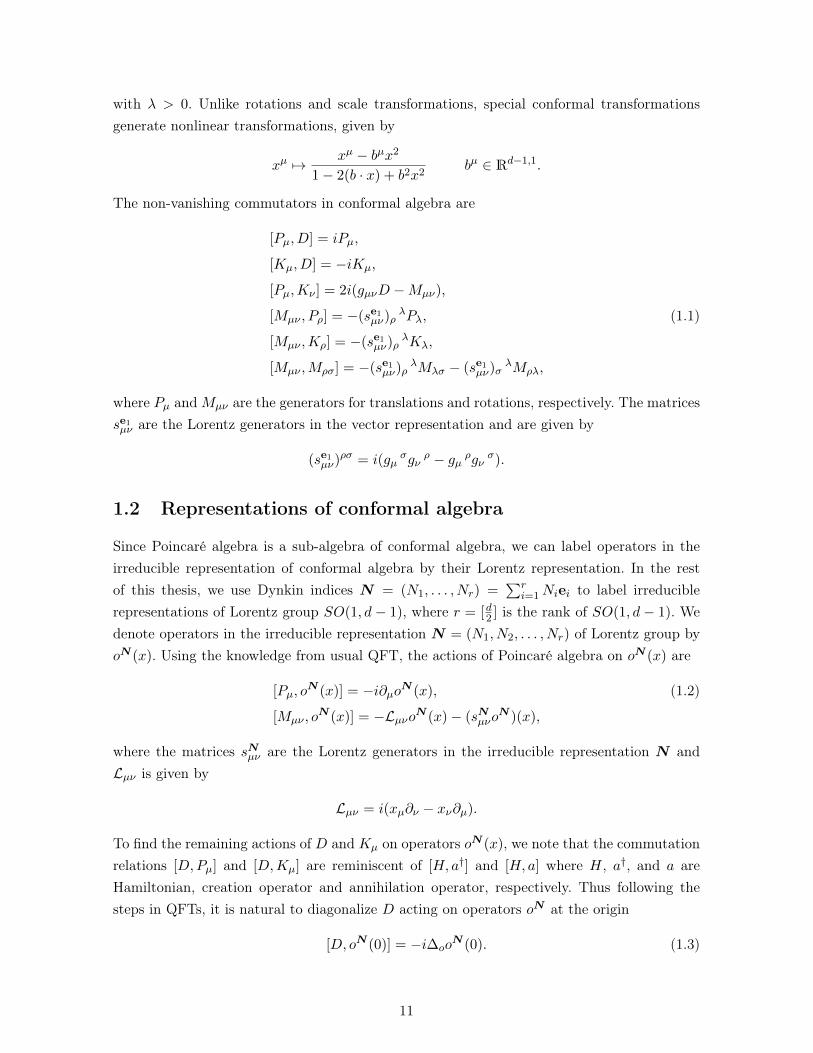
The non-vanishing commutators in conformal algebra are

[Pµ, D] = iPµ,

[Kµ, D] = −iKµ,

[Pµ,Kν ] = 2i(gµνD −Mµν),

[Mµν , Pρ] = −(se1µν)ρ

λPλ, (1.1)

[Mµν ,Kρ] = −(se1µν)ρ

λKλ,

[Mµν ,Mρσ] = −(se1µν)ρ

λMλσ − (se1µν)σ

λMρλ,

where Pµ andMµν are the generators for translations and rotations, respectively. The matricesse1µν are the Lorentz generators in the vector representation and are given by

(se1µν)ρσ = i(gµ

σgνρ − gµ ρgν σ).

1.2 Representations of conformal algebra

Since Poincaré algebra is a sub-algebra of conformal algebra, we can label operators in theirreducible representation of conformal algebra by their Lorentz representation. In the restof this thesis, we use Dynkin indices N = (N1, . . . , Nr) =

∑ri=1Niei to label irreducible

representations of Lorentz group SO(1, d− 1), where r = [d2 ] is the rank of SO(1, d− 1). Wedenote operators in the irreducible representation N = (N1, N2, . . . , Nr) of Lorentz group byoN (x). Using the knowledge from usual QFT, the actions of Poincaré algebra on oN (x) are

[Pµ, oN (x)] = −i∂µoN (x), (1.2)

[Mµν , oN (x)] = −LµνoN (x)− (sNµνo

N )(x),

where the matrices sNµν are the Lorentz generators in the irreducible representation N andLµν is given by

Lµν = i(xµ∂ν − xν∂µ).

To find the remaining actions of D and Kµ on operators oN (x), we note that the commutationrelations [D,Pµ] and [D,Kµ] are reminiscent of [H, a†] and [H, a] where H, a†, and a areHamiltonian, creation operator and annihilation operator, respectively. Thus following thesteps in QFTs, it is natural to diagonalize D acting on operators oN at the origin

[D, oN (0)] = −i∆ooN (0). (1.3)

11

The eigenvalue ∆o is called conformal dimension of oN . The commutation relations in (1.1)tell us that Pµ and Kµ increase and decrease conformal dimensions, respectively. If we as-sume conformal dimensions are bounded from below, then there must exist operators that areannihilated by Kµ, i.e.

[Kµ, oN (0)] = 0. (1.4)

Combining the results in (1.2), (1.3), and (1.4), we define a set of operators called quasi-primary operators by

[Pµ, oN (0)] = −i∂µoN (0),

[Mµν , oN (0)] = −(sNµνo

N )(0), (1.5)

[D, oN (0)] = −i∆ooN (0),

[Kµ, oN (0)] = 0.

We can generate all the other operators of the representation which are called descendants byacting on quasi-primary operators oN (0) with Pµ. In particular, oN (x) = e−ix·P oN (0)eix·P isan infinite linear combination of descendants. The conformal algebra allows us to move awayfrom the origin, leading to the actions on oN(x)

[Pµ, oN (x)] = −i∂µoN (x),

[Mµν , oN (0)] = −LµνoN (x)− (sNµνo

N )(0), (1.6)

[D, oN (0)] = −i(x · ∂ + ∆o)oN (0),

[Kµ, oN (x)] = −i(2xµx · ∂ − x2∂µ + 2∆oxµ)oN (x)− 2xν(sNµνo

N )(x).

1.3 Correlation functions

With the conformal algebra and its representations in hand, we are ready to study the corre-lation functions which are the most natural observables in CFTs. Since the correlation func-tions of descendants can be obtained by acting with Pµ on the correlation functions whichonly contain quasi-primary operators, it is reasonable to focus on the correlation functionsof quasi-primary operators only. In CFTs, the two- and three-point correlation functions arefixed by conformal symmetry up to an overall constant. For instance, the correlation functionsof two and three scalars are

〈o0i (x1)o0j (x2)〉 =Cijδ∆i∆j

x2∆i12

and

〈o0i (x1)o0j (x2)o0k(x3)〉 =Cijk

|x12|∆i+∆j−∆k |x13|∆i+∆k−∆j |x23|∆j+∆k−∆i,

12

with xij = xi − xj . In an unitary CFT, an orthonormal basis of operators can be chosen suchthat two-point correlation functions 〈oN i

i (x1)oNj

j (x2)〉 are proportional to δij . In this thesis,we will always assume that such a basis is chosen.

One can derive the above results by solving conformal Ward identity. Comparing to scalar case,it is much harder to solve the Ward identity for correlation functions of quasi-primary operatorsin generic Lorentz representations. Even for two- and three-point correlation functions, one hasto do tedious computations to obtain the results. As we will see later, the embedding spaceformalism provides an efficient way to compute the correlation functions of quasi-primaryoperators in generic Lorentz representations.

When we go to M > 3-point correlation functions, the situation becomes more complicateddue to the appearance of new conformally invariant variables called conformal cross-ratios.For example, there are two independent conformal cross-ratios that can be built for four-pointcorrelation functions

u =x2

12x234

x213x

224

, v =x2

14x223

x213x

224

.

The number of conformal cross-ratios for four-point correlation functions can be counted asfollows. First, with the help of special conformal transformations, x4 can be sent to infinity.Then we move x1 to the origin by using translations. After that, we fix x3 at (1, 0, . . . , 0) byvirtue of rotations and dilatations. Finally, using rotations that fix x3, we can move x2 to(x, y, 0, . . . , 0), which contains two independent variables x and y, leading to two independentconformal cross-ratios. Following a similar way, one can determine the number of independentconformal cross-ratios Ncr for M -point correlation functions which is given by

Ncr =M(M − 3)

2, M − 3 < d, (1.7)

Ncr = d(M − 3)− (d− 1)(d− 2)

2, M − 3 ≥ d.

The equality in the second line reflects the fact that we do not have enough degrees of freedomto construct M(M − 3)/2 conformal cross-ratios in spacetimes with small d.

Due to the appearance of conformal cross-ratios, M > 3-point correlation functions are morecomplicated objects when comparing with two- and three-point correlation functions. Forinstance, the four-point correlations of four identical scalars have the form

〈o0i (x1)o0i (x2)o0i (x3)o0i (x4)〉 =f(u, v)

x2∆i12 x2∆i

34

, (1.8)

where f is a function of conformal cross-ratios u and v.

1.4 Operator product expansion and conformal blocks

An efficient way to study the function f is using OPE. In CFTs, OPE is one of the most power-ful tools which says that the product between two quasi-primary operators oN i

i (x1)oNj

j (x2)

13

can be re-written as an infinite sum over quasi-primary operators and their descendants. Inother words, we have

oN ii (x1)o

Nj

j (x2) =∑k

Nijk∑a=1

acijkaDij k(x1, x2)oNk

k (x2), (1.9)

where Nijk denotes the number of independent tensor structures inside oN ii (x1)o

Nj

j (x2) ∼oNkk (x2) and the sum over a takes into account all possible tensor structures appearing inthe OPE. acij k are called OPE coefficients which are not fixed by conformal symmetry andencode dynamic information of CFTs. Although OPE coefficients are unconstrained by confor-mal symmetry, they are constrained by crossing symmetry, leading to the celebrated conformalbootstrap. aDij k(x1, x2) are called OPE differential operators whose actions on oNk

k (x2) ge-nerate a proper combination of oNk

k (x2) and its descendants. In principle, aDij k(x1, x2) arecompletely fixed by conformal symmetry. For example, the OPE in one and two dimensionalCFTs has been known for a long time (92; 93; 94; 32), which can be used to prove a set ofFeynman-like rules for writing down all one and two dimensional conformal blocks (91). 1 Inhigher dimensional CFTs, OPE differential operators become complicated due to the nonlinea-rity of conformal group actions. The explicit form of aDij k(x1, x2) for quasi-primary operatorsin generic Lorentz representations is still unknown.

With OPE in hand, any M -point correlation functions can be computed by using OPE repe-titively. For instance, the four-point correlation functions (1.8) can be calculated from OPE

〈{o0i (x1)o0i (x2)}{o0i (x3)o0i (x4)}〉

=∑k

Niik∑a=1

Niik∑b=1

aciikbcii

kaDii k(x1, x2)bDii k(x3, x4)〈oNk

k (x2)oNkk (x4)〉

=∑k

Niik∑a=1

Niik∑b=1

aciikbcii

kabIii

k(x1, x2, x3, x4),

where abIii k(x1, x2, x3, x4) are called conformal partial waves. In the above case, abIii k(x1, x2, x3, x4)

are given by

abIiik(x1, x2, x3, x4) = aDii k(x1, x2)bDii k(x3, x4)〈oNk

k (x2)oNkk (x4)〉.

Comparing with (1.8), we find that f(u, v) can be decomposed as

f(u, v) = x2∆i12 x2∆i

34

∑k

Niik∑a=1

Niik∑b=1

aciikbcii

kabIii

k(x1, x2, x3, x4),

which is dubbed the conformal partial wave decomposition. From conformal partial waves, onecan define the conformal blocks by excluding the leg factors. In the above example, we can

1. We focus on global conformal blocks only.

14

define the four-point conformal blocks abfii k(x1, x2, x3, x4) as

abfiik(x1, x2, x3, x4) =

1

x2∆i12 x2∆i

34

aDii k(x1, x2)bDii k(x3, x4)〈oNkk (x2)oNk

k (x4)〉,

leading to the conformal block decomposition

f(u, v) =∑k

Niik∑a=1

Niik∑b=1

aciikbcii

kabfii

k(x1, x2, x3, x4).

1.5 Embedding space formalism

We know that the action of the conformal algebra on quasi-primary operators is really compli-cated due to the non-linearity of the conformal group. Hence it is better to first linearize theconformal group action. Indeed, the linearization procedure can be implemented by using theisomorphsim between the conformal algebra in Rd−1,1, which we call position space, and theLorentz algebra in Rd,2, which we call embedding space. This is called the embedding spaceformalism. Although the embedding space formalism is often referred as a modern methodto CFT, it was first proposed by Dirac (95) in 1936 and then developed by many physicists(35; 96; 97; 98; 99; 100; 101) . In this embedding space formalism, spinors are quite differentand there is no uniform way to deal with the quasi-primary operators in generic irreducible re-presentations. In this section we will review a different embedding space formalism developedin (61) which gives us a universal way to deal with quasi-primary operators in any irreduciblerepresentation of the Lorentz group SO(d− 1, 1) in position space.

In both embedding space formalism, the embedding space is not the whole Rd,2 but only ahyper-surface i.e, the projective null cone, which satisfies the following conditions 2

η2 = gABηAηB = 0, ληA ∼ ηA λ > 0,

where A ∼ B means that we identify A and B. The coordinates in embedding space and thosein position space are related by

xµ =ηµ

−ηd+1 + ηd+2,

and the conformal generators in embedding space are given by

D = −Ld+1,d+2,

Mµν = Lµν ,

Pµ = −(Lµ,d+1 + Lµ,d+2),

Kµ = Lµ,d+1 − Lµ,d+2,

2. In this thesis, we use x and η to denote position space coordinates and embedding space coordinates,respectively. We also use µ, ν, . . . and α, β, . . . to denote vector and spinor indices of the Lorentz group inposition space as well as A,B, . . . and a, b, . . . to denote vector and spinor indices of the Lorentz group inembedding space.

15

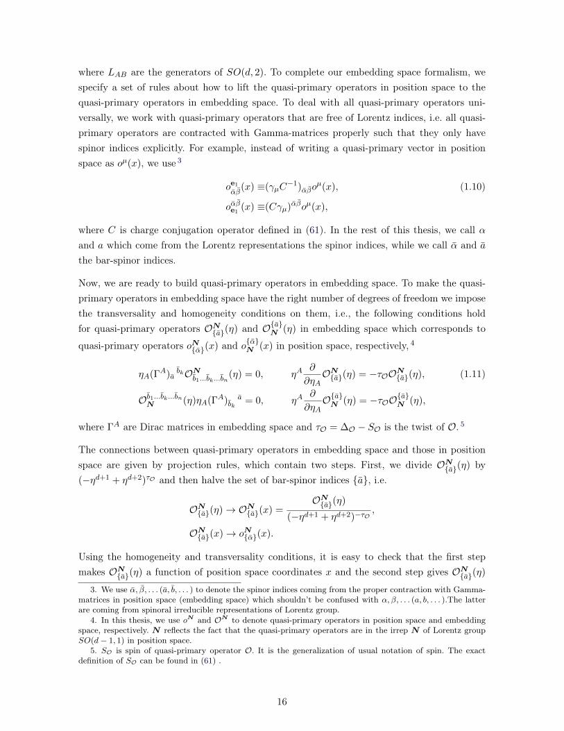
where LAB are the generators of SO(d, 2). To complete our embedding space formalism, wespecify a set of rules about how to lift the quasi-primary operators in position space to thequasi-primary operators in embedding space. To deal with all quasi-primary operators uni-versally, we work with quasi-primary operators that are free of Lorentz indices, i.e. all quasi-primary operators are contracted with Gamma-matrices properly such that they only havespinor indices explicitly. For example, instead of writing a quasi-primary vector in positionspace as oµ(x), we use 3

oe1

αβ(x) ≡(γµC

−1)αβoµ(x), (1.10)

oαβe1(x) ≡(Cγµ)αβoµ(x),

where C is charge conjugation operator defined in (61). In the rest of this thesis, we call αand a which come from the Lorentz representations the spinor indices, while we call α and athe bar-spinor indices.

Now, we are ready to build quasi-primary operators in embedding space. To make the quasi-primary operators in embedding space have the right number of degrees of freedom we imposethe transversality and homogeneity conditions on them, i.e., the following conditions holdfor quasi-primary operators ON

{a}(η) and O{a}N (η) in embedding space which corresponds to

quasi-primary operators oN{α}(x) and o{α}N (x) in position space, respectively, 4

ηA(ΓA)abkON

b1...bk...bn(η) = 0, ηA

∂

∂ηAON{a}(η) = −τOON

{a}(η), (1.11)

Ob1...bk...bnN (η)ηA(ΓA)bka = 0, ηA

∂

∂ηAO{a}N (η) = −τOO{a}N (η),

where ΓA are Dirac matrices in embedding space and τO = ∆O − SO is the twist of O. 5

The connections between quasi-primary operators in embedding space and those in positionspace are given by projection rules, which contain two steps. First, we divide ON

{a}(η) by(−ηd+1 + ηd+2)τO and then halve the set of bar-spinor indices {a}, i.e.

ON{a}(η)→ ON

{a}(x) =ON{a}(η)

(−ηd+1 + ηd+2)−τO,

ON{a}(x)→ oN{α}(x).

Using the homogeneity and transversality conditions, it is easy to check that the first stepmakes ON

{a}(η) a function of position space coordinates x and the second step gives ON{a}(η)

3. We use α, β, . . . (a, b, . . . ) to denote the spinor indices coming from the proper contraction with Gamma-matrices in position space (embedding space) which shouldn’t be confused with α, β, . . . (a, b, . . . ).The latterare coming from spinoral irreducible representations of Lorentz group.

4. In this thesis, we use oN and ON to denote quasi-primary operators in position space and embeddingspace, respectively. N reflects the fact that the quasi-primary operators are in the irrep N of Lorentz groupSO(d− 1, 1) in position space.

5. SO is spin of quasi-primary operator O. It is the generalization of usual notation of spin. The exactdefinition of SO can be found in (61) .

16

the right number of degrees of freedom. To check oN{α}(x) is indeed a quasi-primary operatorin position space, we note that the action of conformal algebra on ON

{a}(x) is simply

[LAB,ON{a}(x)] =[LAB,

ON{a}(η)

(−ηd+1 + ηd+2)−τO]

=(−ηd+1 + ηd+2)τO [LAB,ON{a}(η)]

=− i(−ηd+1 + ηd+2)τO(ηA∂

∂ηB− ηB

∂

∂ηA)ON{a}(η)− (ΣABON ){a}(x)

=− i(ηA∂xµ

∂ηB− ηB

∂xµ

∂ηA)∂

∂xµON{a}(x)− (ΣABON ){a}(x)

+ iτO1

−ηd+1 + ηd+2[ηA(−gB d+1 + gB

d+2)− ηB(−gA d+1 + gAd+2)]ON

{a}(x),

where LAB are generators of Lorentz group in embedding space and ΣAB are proper sums ofgenerators in the fundamental spinor representation. Thus restricting to the first half of thespinor indices of ON

{a}(x) indeed gives us a quasi-primary operator in position space.

To end this section, we give the following important conclusions without proof which saythat a quasi-primary operator oN{α}(x) in position space which belongs to irreducible repre-sentation N = {N1, . . . , Nr} of the Lorentz group SO(d − 1, 1) is lifted to a quasi-primaryoperator ON

{a}(η) in embedding space in an irreducible representation NE = {0, N1, . . . , Nr}of SO(d, 2). The proof can be found in (61).

To simplify the notation, in the remaining parts of this thesis, we will use Oi(η) to representquasi-primary operators in the Lorentz representation N i with the conformal dimension ∆i.

1.6 OPE in the embedding space

In a CFT, once the OPE is known, all correlation functions can be computed by using the OPErecursively. In position space with dimensions larger than two, due to the nonlinearity of theconformal group action, explicit expressions for the OPE involving quasi-primary operators ingeneric Lorentz representations are still unknown. However, the embedding space formalismintroduced in the previous sections makes it possible to write down OPE explicitly in theembedding space as (61)

Oi(η1)Oj(η2) =∑k

Nijk∑a=1

ack

ij aD kij (η1, η2)Ok(η2), (1.12)

where the differential operator aD kij (η1, η2) is

aD kij (η1, η2) =

1

(η1 · η2)pijk(T N i

12 Γ)(T Nj

21 Γ) · at12kij · D

(d,hijk−na/2,na)12 (T12Nk

Γ)∗,

pijk =1

2(τi + τj − τk), hijk = −1

2(χi − χj + χk),

τO = ∆O − SO, χO = ∆O − ξO, ξO = SO − bSOc. (1.13)

17

In the following subsections, we will explain the half-projectors (T Nij Γ) and (TijNΓ) as well as

the differential operator D(d,hijk−na/2,na)12 in (1.13) briefly. More careful and detailed discussions

can be found in (61).

1.6.1 The half-projectors

The half-projectors (T Nij Γ) and (TijNΓ) in (1.13) basically encode the transversality conditions

of the quasi-primary operatorON{a}(ηi) and the way howON

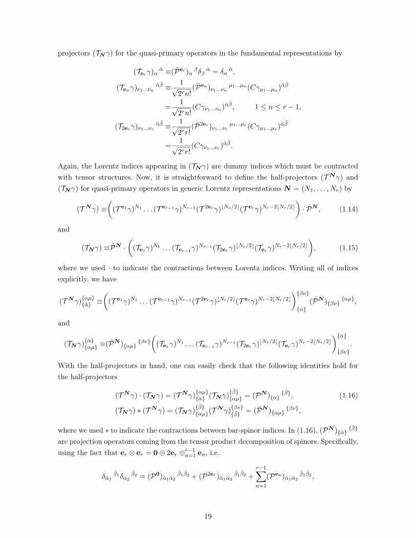
{a}(ηi) transforms under the positionspace Lorentz group SO(d−1, 1). Before going to embedding space, we first introduce the half-projectors in position space. We focus on the fundamental representations including vectors e1,antisymmetric tensors e2≤a≤r−1 and 2er as well as spinors (er) of SO(d−1, 1) (102) 6 since anyirreducible representation can be built from them. The most natural objects that encode theinformation about the Lorentz representation are the projection operators (PN ){αµ}

{βν}. Aswe mentioned before all quasi-primary operators are properly contracted with gamma-matrix,see (1.10). We therefore define the half-projectors (T Nγ) for the quasi-primary operators inthe fundamental representations by

(T erγ)αα ≡δα β(Per)βα = δα

α,

(T enγ)ν1...νnαβ

≡ 1√2rn!

(γµ1...µnC−1)αβ(Pen)µ1...µnν1...νn

=1√2rn!

(γν1...νnC−1)αβ, 1 ≤ n ≤ r − 1,

(T 2erγ)ν1...νrαβ

≡ 1√2rr!

(γµ1...µrC−1)αβ(P2er)µ1...µrν1...νr

=1√2rr!

(γν1...νrC−1)αβ,

where r is the rank of the Lorentz group SO(d− 1, 1) and the fact that

(Per)βα = δβ

α,

(Pen)µ1...µnν1...νn = δ[ν1

µ1 . . . δνn]µn , 1 ≤ n ≤ r − 1,

(P2er)µ1...µrν1...νr = δ[ν1

µ1 . . . δνr]µr

has been used. It seems that the half-projectors still have Lorentz indices as their upperindices. However, as we will see later, these Lorentz indices are dummy indices which mustbe contracted with tensor structures. In a similar way, we define another type of the half-

6. Here, we work in spacetime with odd dimensions. A straightforward generalization exists in even dimen-sions.

18

projectors (TNγ) for the quasi-primary operators in the fundamental representations by

(Terγ)αα ≡(Per)α

βδβα = δα

α,

(Tenγ)ν1...νnαβ ≡ 1√

2rn!(Pen)ν1...νn

µ1...µn(Cγµ1...µn)αβ

=1√2rn!

(Cγν1...νn)αβ, 1 ≤ n ≤ r − 1,

(T2erγ)ν1...νrαβ ≡ 1√

2rr!(P2er)ν1...νr

µ1...µr(Cγµ1...µr)αβ

=1√2rr!

(Cγν1...νr)αβ.

Again, the Lorentz indices appearing in (TNγ) are dummy indices which must be contractedwith tensor structures. Now, it is straightforward to define the half-projectors (T Nγ) and(TNγ) for quasi-primary operators in generic Lorentz representations N = (N1, . . . , Nr) by

(T Nγ) ≡(

(T e1γ)N1 . . . (T er−1γ)Nr−1(T 2erγ)bNr/2c(T erγ)Nr−2bNr/2c)· PN , (1.14)

and

(TNγ) ≡PN ·(

(Te1γ)N1 . . . (Ter−1γ)Nr−1(T2erγ)bNr/2c(Terγ)Nr−2bNr/2c), (1.15)

where we used · to indicate the contractions between Lorentz indices. Writing all of indicesexplicitly, we have

(T Nγ){αµ}{α} ≡

((T e1γ)N1 . . . (T er−1γ)Nr−1(T 2erγ)bNr/2c(T erγ)Nr−2bNr/2c

){βν}{α}

(PN ){βν}{αµ},

and

(TNγ){α}{αµ} ≡(PN ){αµ}

{βν}(

(Te1γ)N1 . . . (Ter−1γ)Nr−1(T2erγ)bNr/2c(Terγ)Nr−2bNr/2c){α}{βν}

.

With the half-projectors in hand, one can easily check that the following identities hold forthe half-projectors

(T Nγ) · (TNγ) = (T Nγ){αµ}{α} (TNγ)

{β}{αµ} = (PN ){α}

{β}, (1.16)

(TNγ) ∗ (T Nγ) = (TNγ){β}{αµ}(T

Nγ){βν}{β} = (PN ){αµ}

{βν},

where we used ∗ to indicate the contractions between bar-spinor indices. In (1.16), (PN ){α}{β}

are projection operators coming from the tensor product decomposition of spinors. Specifically,using the fact that er ⊗ er = 0⊕ 2er ⊕r−1

n=1 en, i.e.

δα1β1δα2

β2 = (P0)α1α2β1β2 + (P2er)α1α2

β1β2 +

r−1∑n=1

(Pen)α1α2β1β2 ,

19

all of the fundamental representations can be built from spinors. As a consequence, we canconstruct any Lorentz representations purely from spinor representations, leading to the pro-jection operators (PN ){α}

{β}. Eq. (1.16) makes it clear why (T Nγ) and (TNγ) are dubbedthe half-projectors.

The definition of the half-projectors in embedding space is more tricky. The issue comesthrough the fact that the half-projectors in embedding space are expected to encode theinformation about the representations of the position space Lorentz group SO(d−1, 1). Due tothis reason, we can not use (PN ){aA}

{bB} since it is the projection operator of the embeddingspace Lorentz group, the full conformal group, SO(d, 2). It is clear that (PN ){αµ}

{βν} and(PN ){aA}

{bB} do not have the same number of degrees of freedom. Indeed, the projectionoperator (PN ){αµ}

{βν} in position space is built from the position space metric gµν , gamma-matrices γµ, charge conjugation operator C and epsilon tensor εµ1...µd , while (PN ){aA}

{bB} isbuilt from the embedding space metric gAB, gamma-matrices ΓA, charge conjugation operatorCΓ and epsilon tensor εA1...Ad+2

, where ΓA and CΓ are given by

Γµ =

(γµ 0

0 −γµ

), Γd+1 = α

(0 1

−α21 0

), Γd+2 = α

(0 1

α21 0

), (1.17)

for α = ±1 (α = ±i) and are purely real (imaginary) if the position space gamma-matrices γare purely real (imaginary), and

CΓ =

(0 C

(−1)r+1C 0

), (1.18)

respectively. To make the half-projectors in embedding space transform like states in the repre-sentation N of the position space Lorentz group SO(d−1, 1), instead of using (PN ){aA}

{bB},we use the projection operator (PN

ij ){aA}{bB} which can be obtained by replacing gAB, ΓA,

εA1...Ad+2in (PN ){aA}

{bB} by the following group-theoretical metric, epsilon tensor and spinorquantities

AABij ≡ gAB −ηAi η

Bj

(ηi · ηj)−

ηBi ηAj

(ηi · ηj), (1.19)

εA1···Adij ≡ 1

(ηi · ηj)ηiA′0ε

A′0A′1···A′dA

′d+1ηjA′d+1

A AdijA′d

· · · A A1

ijA′1,

ΓA1···Anij ≡ ΓA

′1···A′nA An

ijA′n· · · A A1

ijA′1∀n ∈ {0, . . . , r},

which have the appropriate properties (trace, number of vector indices, number of degrees offreedom, etc.) as expected for irreducible representations of the position space Lorentz groupSO(d− 1, 1).

The prescription introduced here does not make the embedding space spinor indices a have theright number of degrees of freedom. However, when projecting to position space, halving thebar-spinor indices a remove extra degrees of freedom. Moreover, we note that the projection

20

operators (PNij ){aA}

{bB} contain two spacetime coordinates ηi and ηj . At first glance, thisseems to be problematic. However in this section we are focusing on the OPE and the OPEalways necessitates using two embedding space coordinates. Hence it is not really an issue touse two spacetime coordinates as long as the OPE is considered.

Now, it seems that the embedding space half-projectors for quasi-primary operators Oen(ηi)

can be defined as

1√2r+1n!

(ΓA1...Anij C−1

Γ )ab,

where r is the rank of the position space Lorentz group SO(d − 1, 1). This is not a properdefinition since we still need to impose the transversality conditions. Instead, we define the em-bedding space half-projectors for quasi-primary operators in the fundamental representationsof SO(d− 1, 1) as

(T erij Γ)aa ≡

1√2ηi · ηj

(ηi · Γηj · Γ)aa,

(T enij Γ)A1...An

ab≡

√n+ 1

√2r+1n!(ηi · ηj)

12

(ηiA0ΓA0A1...Anij C−1

Γ )ab, 1 ≤ n ≤ r − 1,

(T 2erij Γ)A1...Ar

ab≡

√r + 1

√2r+1r!(ηi · ηj)

12

(ηiA0ΓA0A1...Arij C−1

Γ )ab,

and

(TijerΓ)aa ≡ 1√

2ηi · ηj(ηj · Γηi · Γ)a

a,

(TijenΓ)abA1...An ≡√n+ 1

√2r+1n!(ηi · ηj)

12

(ηiA0CΓΓijA0A1...An)ab, 1 ≤ n ≤ r − 1,

(Tij2erΓ)abA1...Ar ≡√r + 1

√2r+1r!(ηi · ηj)

12

(ηiA0CΓΓijA0A1...Ar)ab,

respectively. They verify the transversality conditions through the fact that (ηi ·Γ)ab(ηi ·Γ)b

c =

ηi · ηiδca = 0. We stress that we define (T erij Γ)aa ∝ ηi · Γηj · Γ instead of (T er

ij Γ)aa ∝ ηi · Γ sincethe latter vanishes after halving the bar-spinor index. In other words, ηi · Γ projects to 0 byusing the projection rules.

Now, it is straightforward to define the embedding space half-projectors (T Nij Γ) and (TijNΓ)

for quasi-primary operators ON (ηi) in generic Lorentz representations N = (N1, . . . , Nr) by

(T Nij Γ) ≡

((T e1ij Γ)N1 . . . (T er−1

ij Γ)Nr−1(T 2erij Γ)bNr/2c(T er

ij Γ)Nr−2bNr/2c)· PN

ij , (1.20)

and

(TijNΓ) ≡PNji ·

((Tije1Γ)N1 . . . (Tijer−1Γ)Nr−1(Tij2erΓ)bNr/2c(TijerΓ)Nr−2bNr/2c

). (1.21)

21

The half-projectors (T Nij Γ) and (TijNΓ) satisfy

(TijNΓ){aA} ∗ (T Njk Γ){Bb} =

(ηi · ηj)12

(S−ξ)

(ηj · ηk)12

(S−ξ)

((ηj · Γ)2ξ PN

ji · PNjk (ηk · Γ)2ξ

(ηj · ηk)2ξ

) {Bb}

{aA}

,

which can be thought as a generalization of the second equality in (1.16) in embedding space.

1.6.2 The OPE differential operator D(d,h,n)12

Since the OPE represents the product of two quasi-primary operators in terms of an infinitesum over quasi-primary operators and their descendants, the OPE differential operators areneeded to generate conformal descendants by acting on the quasi-primary operators. Althoughthe OPE differential operator is completely fixed by conformal symmetry, an explicit expressionof the position space OPE differential operator in any dimension d is still missing. In contrastto the position space OPE differential operator, the embedding space OPE differential operatoris strongly restricted by the light-cone condition (15; 59; 61; 103; 104; 105; 106; 107; 108; 109).Specifically, besides generating descendants, the OPE differential operator in embedding spacemust be well-defined on the light-cone. In other words, the action of the embedding space OPEdifferential operator on any smooth function f(η) = η2g(η) must vanish on the light-cone.

The light-cone condition and the fact that the OPE differential operators generate conformaldescendants narrow the possible candidates for the embedding space OPE differential operatorto a single one D(d,hijk−na/2,na)

12 in (1.13) (61). Following the discussions in (61), D(d,h,n)ij is the

most convenient differential operator which can be used in the embedding space OPE whichhas n vector indices, given by

D(d,h,n)ij ≡ D(d,h,n)F1...Fn

ij =1

(ηi · ηj)n2

D2(h+n)ij ηF1

j . . . ηFnj , (1.22)

where

D2(h+n)ij = (D2

ij)h+n = (gF1F2D

F1ij D

F2ij )h+n,

DFij = (ηi · ηj)12AFF ′ij

∂

∂ηF′

j

.

These differential operators satisfy several commutation relations

[DFij ,D2hij ] =

2h

(ηi · ηj)12

ηFi D2hij , [Θi,D2h

ij ] = hD2hij , [Θj ,D2h

ij ] = −hD2hij ,

D2hij η

Fj − η

Fj D

2hij = 2h(ηi · ηj)

12DFijD

2(h−1)ij − h(d+ 2h− 2)ηFi D

2(h−1)ij ,

where Θ is the homogeneity operator defined by

Θ = ηA∂

∂ηA.

22

It is easy to check that D(d,h,n)ij is fully symmetric and traceless with respect to the embedding

space metric g, which implies that the differential operator D(d,h,n)ij corresponds to the Dynkin

index ne1 of the appropriate symmetric-traceless irreducible representation under considera-tion. (1.22) also implies the following important identity for D(d,h,n)

ij

D(d,h,n)F1···Fnij η

Fn+1

j · · · ηFn+k

j = (ηi · ηj)k2D(d,h−k,n+k)F1···Fn+k

ij .

As a result, free ηj ’s appearing in computations can be properly taken into account withthe differential operator D(d,h,n)

ij , which is useful for computations of the correlation functionsinvolving spinning quasi-primary operators.

1.6.3 Tensor structures

The last ingredients in the embedding space OPE (1.12) and (1.13) are tensor structures.These are purely group theoretic quantities that are entirely determined by the irreduciblerepresentations of the quasi-primary operators in question. In the OPE (1.12) and (1.13), thereare four set of dummy indices which can be seen as originating from four different irreduciblerepresentations of the Lorentz group. Three of them come from the half-projectors (T N i

12 Γ),(T Nj

21 Γ), and (T12NkΓ). The fourth comes from the OPE differential operator D(d,h,n)

ij . Tomatch the free indices in the OPE, these dummy indices must be properly contracted, whichcan be implemented by contracting with tensor structures at12k

ij . The different tensor structuresappear to contract the four sets of dummy variables into a Lorentz singlet. Thus, for threequasi-primary operators in specific Lorentz representations N i, N j and Nk, the number oftensor structures at12k

ij , i.e. the number Nijk denoting the range of the sum over a in (1.12),is equal to the number of Lorentz singlet appearing in the tensor product decomposition of

N i ⊗N j ⊗Nk ⊗ symmetric-traceless irreps.

We note that the tensor product decomposition of N and symmetric-traceless representationscontains Lorentz singlet only when N are also symmetric-traceless representations. We there-fore conclude that the number of tensor structures at12k

ij is given by the number of symmetric-traceless representations appearing in the tensor product decomposition of N i ⊗N j ⊗Nk.From the OPE (1.12), this fact implies that there areNijk independent OPE coefficients ac

kij . 7

It is worth stressing here that all irreducible representations involved in the discussion abouttensor structures are representations of the position space Lorentz group SO(d−1, 1) instead ofthe full conformal group SO(d, 2). Analogy to the half-projectors and projection operators inembedding space, there exists a one-to-one map between the embedding space tensor structures

at12kij and the position space tensor structures. Specifically, tensor structures in embedding

7. When one or more quasi-primary operators become conserved, conservation conditions further reducethe number of independent OPE coefficients. The embedding space formalism introduced in this chapter alsoprovides an efficient and systematical way to study the conservation conditions (110).

23

space are obtained from their position space counterparts by making the substitutions in (1.19).By constructions, these exhibit all the desired properties to guarantee proper contraction withthe corresponding irreducible representations of the position space Lorentz group.

1.7 Correlation functions from OPE

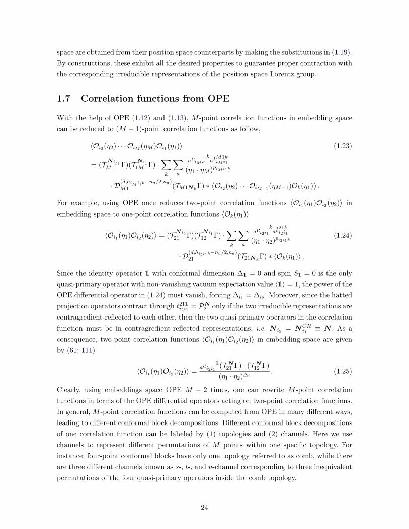
With the help of OPE (1.12) and (1.13), M -point correlation functions in embedding spacecan be reduced to (M − 1)-point correlation functions as follow,

〈Oi2(η2) · · · OiM (ηM )Oi1(η1)〉 (1.23)

= (T N iMM1 Γ)(T N i1

1M Γ) ·∑k

∑a

ack

iM i1 atM1kiM i1

(η1 · ηM )piM i1k

· D(d,hiM i1k−na/2,na)

M1 (TM1NkΓ) ∗

⟨Oi2(η2) · · · OiM−1(ηM−1)Ok(η1)

⟩.

For example, using OPE once reduces two-point correlation functions 〈Oi1(η1)Oi2(η2)〉 inembedding space to one-point correlation functions 〈Ok(η1)〉

〈Oi1(η1)Oi2(η2)〉 = (T N i221 Γ)(T N i1

12 Γ) ·∑k

∑a

ack

i2i1 at21ki2i1

(η1 · η2)pi2i1k(1.24)

· D(d,hi2i1k−na/2,na)

21 (T21NkΓ) ∗ 〈Ok(η1)〉 .

Since the identity operator 1 with conformal dimension ∆1 = 0 and spin S1 = 0 is the onlyquasi-primary operator with non-vanishing vacuum expectation value 〈1〉 = 1, the power of theOPE differential operator in (1.24) must vanish, forcing ∆i1 = ∆i2 . Moreover, since the hattedprojection operators contract through t211

i2i1= PN

21 only if the two irreducible representations arecontragredient-reflected to each other, then the two quasi-primary operators in the correlationfunction must be in contragredient-reflected representations, i.e. N i2 = NCR

i1 ≡ N . As aconsequence, two-point correlation functions 〈Oi1(η1)Oi2(η2)〉 in embedding space are givenby (61; 111)

〈Oi1(η1)Oi2(η2)〉 =ac

1i2i1

(T N21 Γ) · (T N

12 Γ)

(η1 · η2)∆i. (1.25)

Clearly, using embeddings space OPE M − 2 times, one can rewrite M -point correlationfunctions in terms of the OPE differential operators acting on two-point correlation functions.In general, M -point correlation functions can be computed from OPE in many different ways,leading to different conformal block decompositions. Different conformal block decompositionsof one correlation function can be labeled by (1) topologies and (2) channels. Here we usechannels to represent different permutations of M points within one specific topology. Forinstance, four-point conformal blocks have only one topology referred to as comb, while thereare three different channels known as s-, t-, and u-channel corresponding to three inequivalentpermutations of the four quasi-primary operators inside the comb topology.

24

The knowledge of the embedding space OPE (1.12) and (1.13) allows us to compute M -pointconformal blocks with different topologies and channels. For example, iterating (1.23) M − 2

times, one can rewrite M -point correlation functions in terms of conformal blocks with combtopology

〈Oi2(η2) · · · OiM (ηM )Oi1(η1)〉

=

M−2∏j=1

(TN iM−j+1

M−j+1,1 Γ)(TNkM−j+1

1,M−j+1 Γ)∑kM−j

∑aM−j

aM−jckM−j

iM−j+1kM−j+1

(η1 · ηM−j+1)pM−j+1

·aM−j tM−j+1,1kM−jiM−j+1kM−j+1

· D(d,hM−j−naM−j /2,naM−j )

M−j+1,1 (TM−j+1,1NkM−jΓ)∗]〈Ok2(η2)Ok1(η1)〉 ,

where

pM−j+1 =1

2(τiM−j+1 + τkM−j+1

− τkM−j ), hM−j = −1

2(χiM−j+1 − χkM−j+1

+ χkM−j ),

and kM = i1.

Since M -point conformal blocks can be computed by acting OPE differential operators onlower-point conformal blocks, it is necessary to obtain the actions of OPE differential operatorson correlation functions. In general, the computation of M -point correlation functions fromthe OPE leads to the study of the tensorial functions

I(d,h,n;p)A1···Anij = D(d,h,n)A1···An

ij

∏a6=i,j

1

(ηj · ηa)pa.

For M -point correlation functions at embedding space coordinates η1 to ηM , the product overa runs from 1 to M . We take a 6= i, j due to the fact that powers of (ηi · ηj) commute withD(d,h,n)ij and that (ηj · ηj) = 0. In practice, it is alway useful to define the I-function which

can be obtained by properly homogeneizing the above I-function. Since the homogenizationof I-functions for three- and M > 3-point correlation functions are slightly different, we dealwith them separately. The remaining part of this section will give an explicit expression of theI-function without any proof. More careful and detailed discussions can be found in (61).

1.7.1 Three-point tensorial function

For three-point correlation functions, we define the I-function as

I(d,h,n;p)12 =

(η2 · η3)p+h+n2

(η1 · η3)h+n2

D(d,h,n)12

1

(η2 · η3)p, (1.26)

where we chose the three coordinates as η1, η2, and η3. The three-point tensorial function wasfound in (60; 61) and is given explicitly by

I(d,h,n;p)12 = ρ(d,h;p)

∑q0,q1,q2,q3≥0

q=2q0+q1+q2+q3=n

S(q0,q1,q2,q3)K(d,h;p;q0,q1,q2,q3), (1.27)

25

where the totally symmetric S-tensor, the ρ-function, and the K-function are

SA1···Aq(q0,q1,q2,q3) = g(A1A2 · · · gA2q0−1A2q0 ¯η

A2q0+1

1 · · · ¯ηA2q0+q11

× ¯ηA2q0+q1+1

2 · · · ¯ηA2q0+q1+q22

¯ηA2q0+q1+q2+1

3 · · · ¯ηAq)3 ,

ρ(d,h;p) = (−2)h(p)h(p+ 1− d/2)h,

K(d,h;p;q0,q1,q2,q3) =(−1)q−q0−q1−q2(−2)q−q0 q!

q0!q1!q2!q3!

(−h− q)q−q0−q2(p+ h)q−q0−q1(p+ 1− d/2)−q0−q1−q2

,

For three-point tensorial function, the homogeneized embedding space coordinates ¯η1, ¯η2, and¯η3 are

¯ηA1 =(η2 · η3)

12

(η1 · η2)12 (η1 · η3)

12

ηA1 , ¯ηA2 =(η1 · η3)

12

(η1 · η2)12 (η2 · η3)

12

ηA2 , ¯ηA3 =(η1 · η2)

12

(η1 · η3)12 (η2 · η3)

12

ηAa .

Using the definition (1.26), it is straightforward to check that the three-point tensorial functionI

(d,h,n;p)12 is totally symmetric and traceless with respect to the embedding space metric g andit also satisfies several contiguous relations (60; 61), given by

g · I(d,h,n;p)12 = 0,

¯η1 · I(d,h,n;p)12 = I

(d,h+1,n−1;p)12 ,

¯η2 · I(d,h,n;p)12 = ρ(d,1;−h−n)I

(d,h,n−1;p)12 ,

¯η3 · I(d,h,n;p)12 = I

(d,h+1,n−1;p−1)12 .

Equipped with the three-point tensorial function, all three-point correlation functions in em-bedding space can be obtained through the embedding space OPE (112).

M > 3-Point Tensorial Function

The definition of M > 3-point I-function is different due to the existence of more embeddingspace coordinates. According to (61), without introducing any powers of (ηj ·ηa) for all a 6= i, j,the homogeneizing procedure of M > 3-point I-function can be implemented by using twoextra embedding space coordinates ηk and η`. The M > 3-point tensorial function is definedas

I(d,h,n;p)ij;k` =

(ηi · ηj)p+h+n2 (ηk · η`)p+h+n

2

(ηi · ηk)p+h+n2 (ηi · η`)p+h+n

2

∏a6=i,j

(ηi · ηa)pa I(d,h,n;p)

ij , (1.28)

with k < ` and k, ` 6= i, j and p =∑

a6=i,j pa. Another new feature forM > 3 tensorial functionis the appearance of conformal cross-ratios. Using the two extra embedding space coordinates

26

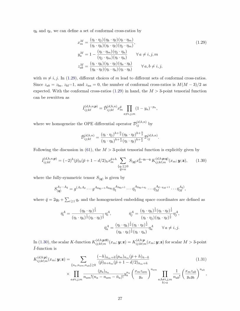
ηk and η`, we can define a set of conformal cross-ratios by

xMm =(ηi · ηj)(ηk · η`)(ηi · ηm)

(ηi · ηk)(ηi · η`)(ηj · ηm), (1.29)

yMa = 1− (ηi · ηm)(ηj · ηa)(ηj · ηm)(ηi · ηa)

∀ a 6= i, j,m

zMab =(ηi · ηk)(ηi · η`)(ηa · ηb)(ηk · η`)(ηi · ηa)(ηi · ηb)

∀ a, b 6= i, j,

with m 6= i, j. In (1.29), different choices of m lead to different sets of conformal cross-ratios.Since zab = zba, zkl=1, and zaa = 0, the number of conformal cross-ratios is M(M − 3)/2 asexpected. With the conformal cross-ratios (1.29) in hand, the M > 3-point tensorial functioncan be rewritten as

I(d,h,n;p)ij;k` = D(d,h,n)

ij;k` xpm∏

a6=i,j,m(1− ya)−pa ,

where we homogeneize the OPE differential operator D(d,h,n)ij by

D(d,h,n)ij;k` =

(ηi · ηj)h+n2 (ηk · η`)h+n

2

(ηi · ηk)h+n2 (ηi · η`)h+n

2

D(d,h,n)ij .

Following the discussion in (61), the M > 3-point tensorial function is explicitly given by

I(d,h,n;p)ij;k` = (−2)h(p)h(p+ 1− d/2)hx

p+hm

∑{qr}≥0q=n

S(q)xq−q0−qim K

(d,h;p;q)ij;k`;m (xm;y; z), (1.30)

where the fully-symmetric tensor S(q) is given by

SA1···Aq(q) = g(A1A2 · · · gA2q0−1A2q0 η

A2q0+1

1 · · · ηA2q0+q11 · · · ηAq−qM+1

M · · · ηAq)M ,

where q = 2q0 +∑

r≥1 qr and the homogeneized embedding space coordinates are defined as

ηAi =(ηk · η`)

12

(ηi · ηk)12 (ηi · η`)

12

ηAi , ηAj =(ηi · ηk)

12 (ηi · η`)

12

(ηi · ηj)(ηk · η`)12

ηAj ,

ηAa =(ηi · ηk)

12 (ηi · η`)

12

(ηk · η`)12 (ηi · ηa)

ηAa ∀ a 6= i, j.

In (1.30), the scalarK-functionK(d,h;p;0)ij;k`;m (xm;y; z) = K

(d,h;pij;k`;m(xm;y; z) for scalarM > 3-point

I-function is

K(d,h;p)ij;k`;m(xm;y; z) =

∑{na,nam,nab}≥0

(−h)nm+¯n(pm)nm(p+ h)n−¯n

(p)n+nm(p+ 1− d/2)nm+¯n(1.31)

×∏

a6=i,j,m

(pa)nanam!(na − nam − na)!

ynaa

(xmzamya

)nam ∏a,b 6=i,j,mb>a

1

nab!

(xmzabyayb

)nab,

27

where we have defined

n =∑

1≤a≤Ma6=i,j,m

na, nm =∑

1≤a≤Ma6=i,j,m

nam,

na =∑

1≤b≤Mb6=i,j,m,a

nab, ¯n =∑

1≤a<b≤Ma,b 6=i,j,m

nab.

By recurrence, one finds the tensorial K-function K(d,h;p;q)ij;k`;m (xm;y; z) is

K(d,h;p;q)ij;k`;m =

(−1)q−q0−qi−qj (−2)q−q0 q!∏r≥0 qr!

(−h− q)q−q0−qj (pm)qm(p+ h)q−q0−qi(p)q−2q0−qi−qj (p+ 1− d/2)−q0−qi−qj

∏a6=i,j,m

(pa)qa

×K(d+2q−2q0,h+q0+qj ;p+q)ij;k`;m ,

where it is understood that q in p+q does not include the zeroth, the i-th and j-th componentsq0, qi and qj respectively. Hence, the tensorial K-function is given by the scalar K-functionK

(d,h;p)ij;k`;m(xm;y; z) with properly shifted parameters.

For M = 4, the scalar K-function K(d,h;p)ij;k`;m(xm;y; z) is exactly the Exton G-function for four-

point scalar conformal blocks with scalar exchanges (113), given by

K(d,h;p3,p4)12;34;3 (x3; y4) =

∑n4,n34≥0

(−h)n34(p3)n34(p3 + p4 + h)n4

(p3 + p4)n4+n34(p3 + p4 + 1− d/2)n34

(p4)n4

n34!(n4 − n34)!yn4

4

(x3

y4

)n34

= G(p4, p3 + p4 + h, p3 + p4 + 1− d/2, p3 + p4;u/v, 1− 1/v),

where the conformal cross-ratios are

u =(η1 · η2)(η3 · η4)

(η1 · η3)(η2 · η4), v =

(η1 · η4)(η2 · η3)

(η1 · η3)(η2 · η4).

The tensorial K-function allows us to obtain four-point conformal blocks with external andinternal quasi-primary operators in generic Lorentz representations (62; 63).

For M > 4, it is the proper generalization of the Exton G-function to M -point correlationfunctions. In the next chapter, we will use M > 4-point scalar K-function to compute somespecific conformal blocks with external and internal scalars, including M -point conformalblocks with comb topology, six-point conformal blocks with snowflake topology as well asseven-point conformal blocks with extended snowflake topology.

28

Chapitre 2

Higher-Point Conformal Blocks fromEmbedding Space OPE

In this chapter, we will use the techniques developed in Chapter 1 to study some specificM > 4-point scalar conformal blocks with scalar exchanges. This chapter is based on publishedpapers (79; 80; 81) in which I did almost all of the computations. Since the embedding spaceOPE for two quasi-primary scalars with scalar exchanges and the scalar I-function are usedautocratically in this chapter, we repeat them here

Oi(η1)Oj(η2) = c kij

1

(η1 · η2)pijkD(d,hijk,0)

12 Ok(η2) + . . . , (2.1)

pijk =1

2(∆i + ∆j −∆k), hijk = −1

2(∆i −∆j + ∆k),

where in the first line we omitted non-scalar primary operators and 1

D2hij;kl;mx

qm

∏1≤a≤Ma6=i,j,m

(1− ya)−qa (2.2)

= xq+hm

∑{na,nam,nab}≥0

(−h)nm+¯n(qm)nm(q + h)n−¯n

(q)n+nm(q + 1− d/2)nm+¯n

×∏

1≤a≤Ma6=i,j,m

(qa)nanam!(na − nam − na)!

ynaa

(xmzamya

)nam ∏1≤a<b≤Ma,b 6=i,j,m

1

nab!

(xmzabyayb

)nab,

1. For simplicity, we omit the pre-factor (−2)h(q)h(q + 1 − d/2)h which is an overall constant and can beabsorbed into the OPE coefficients.

29

where we have defined q =∑

1≤a≤Ma6=i,j

qa as well as

n =∑

1≤a≤Ma6=i,j,m

na, nm =∑

1≤a≤Ma6=i,j,m

nam,

na =∑

1≤b≤Mb6=i,j,m,a

nab, ¯n =∑

1≤a<b≤Ma,b 6=i,j,m

nab.

Equipped with the embedding space OPE, one can compute M -point conformal blocks withany topology by acting with the OPE properly on (M−1)-point conformal blocks. In practice,the strategy to compute arbitrary M -point conformal blocks is made out of the following foursteps. (1) Re-express the (M − 1)-point conformal blocks in terms of the conformal cross-ratios xM−1

m , yM−1a , and zM−1

ab in (1.29). (2) Act on the (M − 1)-point conformal blocks withOPE and write the desired M -point conformal blocks in terms of K-function by using (2.2).(3) Re-express the conformal cross-ratios xMm , yMa , and zMab in terms of an appropriate set ofconformal cross-ratios uMa and vMab . (4) Compute summations, leading to a relatively simpleresult for the M -point conformal blocks. In principle, one can obtain a result for M -pointconformal blocks in terms of conformal cross-ratios xMm , yMa , and zMab after performing step(2), which contains several superfluous sums. Step (3) and (4) are performed to simplify theresult. It is noteworthy that the best choice of conformal cross-ratios uMa and vMab is not knowna priori (there are usually more than one) and that they are dependent on the topology.All re-summations in step (4) rely on identities involving hypergeometric functions 2F1 andgeneralized hypergeometric functions 3F2 , given by

2F1

[−n, bc

; 1

]=

(c− b)n(c)n

, (2.3)

and

3F2

[−n, b, cd, e

; 1

]=

(d− b)n(d)n

3F2

[−n, b, e− c

b− d− n+ 1, e; 1

], (2.4)

3F2

[−n, b, c

d, 1 + b+ c− d− n; 1

]=

(d− b)n(d− c)n(d)n(d− b− c)n

,

for n a non-negative integer.

Before computing specific higher-point conformal blocks, let us introduce some convenientnotations. In general, it is possible to write the conformal partial wave with external andexchanged scalar quasi-primary operators, from a specific topology, as

I(∆i2

,...,∆iM,∆i1

)

M(∆k1,...,∆kM−3

)

∣∣∣∣topology

= L(∆i2

,...,∆iM,∆i1

)

M |channel

∏1≤a≤M−3

(uMa )∆ka

2

G(d,h;p)M |topology(uM ,vM ).

(2.5)

30

The scalar M -point conformal block with scalar exchanges is given by 2

G(d,h;p)M |channel(u

M ,vM ) =∑

{ma,mab}≥0

C(d,h;p)M |channel(m,m)F

(d,h;p)M |channel(m,m) (2.6)

×∏

1≤a≤M−3

(uMa )ma

ma!

∏1≤a≤b≤M−3

(1− vMab )mab

mab!.

In (2.5) and (2.6) ∆ia and ∆ka are the conformal dimensions of the external scalar quasi-primary operators and the conformal dimensions of the exchanged scalar quasi-primary ope-rators, respectively. Moreover, the legs LM are made out of embedding space coordinateswhich encode desired scaling behaviours of the conformal partial wave. Like the conformalcross-ratios uMa and vMab , the best choice of the legs LM is not known a priori and they are alsodependent on the topology. The scalar M -point conformal blocks (2.6) are written as sumsover powers of conformal cross-ratios, with extra sums denoted by the function FM . In general,FM could be a function of both the vector m = (ma) and the matrix m = (mab). Thus theseparation between CM and FM is somewhat arbitrary in (2.6). As we will see in this chapter,FM with the comb topology, F6 with the snowflake topology, and F7 with the extended snow-flake topology are only functions of the vector m. That statement seems to generalize to allFM , thus we conjecture that FM can always be chosen such that it is a function of the vectorm only. Finally, in the scalar M -point conformal blocks (2.6) the vectors h and p are somelinear combinations of the conformal dimensions ∆ia and ∆ka , originated from the OPE (2.1).

In our notation, the statement that arbitrary M -point conformal blocks can be obtained fromthe (M − 1)-point conformal blocks by acting with the OPE properly translates into 3

I(∆i2

,...,∆iM,∆i1

)

M(∆k1,...,∆kM−3

)

∣∣∣∣topology

=1

ηpM1M

(ηkMηlMη1Mηkl

)hM−1

D2hM−1

M1;kl I(∆i2

,...,∆iM−1,∆kM−3

)

M−1(∆k1,...,∆kM−4

)

∣∣∣∣topology

,

(2.7)

where we have defined ηab ≡ (ηa · ηb) and the appropriate topology on the RHS has beenchosen to generate the desired topology on the LHS. For future convenience, we also definepa =

∑ab=2 pb and ha =

∑ab=2 hb.

In the next few sections, we will use the strategy mentioned in the beginning of this chapterto compute M -point conformal blocks with the comb topology, six-point conformal blockswith the snowflake topology as well as seven-point conformal blocks with the extended snow-flake topology. In Appendix A, we show a complete computation for deriving scalar five-pointconformal blocks of (77) by using our OPE strategy. The computations for deriving otherhigher-point conformal blocks discussed in this chapter are analogous but tedious.

2. The conformal block gM defined in Chapter 1 is given by gM =

[∏1≤a≤M−3(uMa )

∆ka2

]GM .

3. Without loss of generality, we always choose the OPE differential operator acting on embedding spacecoordinates η1.

31

I(∆i2

,...,∆iM,∆i1

)

M(∆k1,...,∆kM−3

)= Oi2 Oi1

Oi3 Oi4· · ·

OiM−1 OiM

Ok1OkM−3

Figure 2.1 – Conformal blocks with the comb topology.

2.1 M-point conformal blocks with the comb topology

M -point scalar conformal blocks with scalar exchanges are depicted in Fig 2.1, which can beobtained by acting OPE repetitively as follows

I(∆i2

,...,∆iM,∆i1

)

M(∆k1,...,∆kM−3

)

∣∣∣∣comb

=

M−2∏j=1

∑kM−j

ciM−j+1kM−j+1kM−j

(η1 · ηM−j+1)pM−j+1D(d,hM−j ,0)M−j+1,1

〈Ok2(η2)Ok1(η1)〉 ,

(2.8)

where

pM−j+1 =1

2(τiM−j+1 + τkM−j+1

− τkM−j ), hM−j = −1

2(χiM−j+1 − χkM−j+1

+ χkM−j ),

and kM = i1. In principle, the above M -point comb blocks can be obtained by starting fromthe two-point function 〈Ok2(η2)Ok1(η1)〉 and repeating our strategy mentioned earlier M − 2

times, which is apparently impractical. Instead, a more efficient way, which will be used here,is to solve recursion relations. Specifically, we first derive recursion relations which connect IMwith IM−1 by using the strategy once and then solve them by substituting the known resultfor I4.

To proceed, we first introduce the legs LM as well as a set of conformal cross-ratios uMa andvMab as

LM |comb =

(ηM−1,M

η1,M−1η1M

)∆i1/2( η34

η23η24

)∆i2/2 ∏

1≤a≤M−2

(ηa+1,a+3

ηa+1,a+2ηa+2,a+3

)∆ia+2/2

, (2.9)

and

uMa =(η1+a · η2+a)(η3+a · η4+a)

(η1+a · η3+a)(η2+a · η4+a), 1 ≤ a ≤M − 3, (2.10)

vMab =(η2−a+b · η4+b)

(η2+b · η4+b)

∏1≤c≤a

(η3+b−c · η4+b−c)

(η2+b−c · η4+b−c), 1 ≤ a ≤ b ≤M − 3,

32

with ηM+1 ≡ η1. Moreover, we also take C(d,h;p)M |comb(m,m) as

C(d,h;p)M |comb(m,m) =

(p3)m1+tr0m(p2 + h2)m1+tr1m

(p3)m1+tr1mF

(d,h;p)M (m) (2.11)

×

∏1≤a≤M−3

(pa+2 −ma−1)ma+tram(pa+2 + ha+2)ma+ma+1+ma+ ¯ma

(pa+2 + ha+1)2ma+ma−1+ma+ ¯ma

×(−ha+2)ma(−ha+2 +ma −ma+1)ma−1

(pa+2 + ha+1 + 1− d/2)ma

]with

tram =∑b

mb,a+b, ma =∑b≤a

mba, ¯ma =∑b>a

(mb − trbm).

We stress that the choice of C(d,h;p)M |comb(m,m) in (2.11) is always possible since we keep FM |comb

arbitrary. The quantities p and h, which are related to the OPE differential operators inembedding space (2.1), are given explicitly in terms of the conformal dimensions by

p2 = ∆i3 , 2p3 = ∆i2 + ∆k1 −∆i3 , 2pa = ∆ia + ∆ka−2 −∆ka−3 ,

2h2 = ∆k1 −∆i2 −∆i3 , 2ha = ∆ka−1 −∆ka−2 −∆ia+1 ,

with kM−2 = i1, pa =∑a

b=2 pb and ha =∑a

b=2 hb.

With the legs (2.9), conformal cross-ratios (2.10), and C-function (2.11) in hand, we cantranslate the recursion relation for IM |comb into the recursion relation for FM |comb. Now, letus follow our strategy to derive the desired recursion relations.

We first choose k = 2, ` = 3, and m = 2, leading to

xM2 =η1Mη23

η12η3M, (2.12)

yMa = 1− η1aη2M

η12ηaM, 3 ≤ a ≤M − 1,

zMab =ηabη2Mη3M

η23ηaMηbM, 2 ≤ a < b ≤M − 1.

Following step (1), we re-express the conformal cross-ratios uM−1a and vM−1

ab in terms of xM2 ,yMa , and zMab in (2.12), given by

uM−1M−4 =

1− yMM−1

1− yMM−2

zMM−3,M−2

zMM−3,M−1

,

vM−1a,M−4 =

1− yMM−2−a1− yMM−2

∏1≤b≤a

zMM−2−a+b,M−1−a+b

zMM−3−a+b,M−1−a+b

.

33

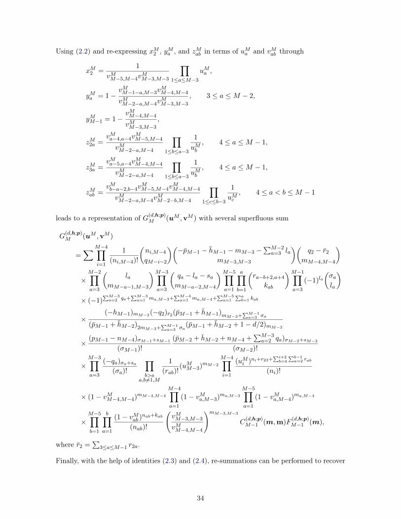
Using (2.2) and re-expressing xM2 , yMa , and zMab in terms of uMa and vMab through

xM2 =1

vMM−5,M−4vMM−3,M−3

∏1≤a≤M−3

uMa ,

yMa = 1−vMM−1−a,M−3v

MM−4,M−4

vMM−2−a,M−4vMM−3,M−3

, 3 ≤ a ≤M − 2,

yMM−1 = 1−vMM−4,M−4

vMM−3,M−3

,

zM2a =vMa−4,a−4v

MM−5,M−4

vMM−2−a,M−4

∏1≤b≤a−3

1

uMb, 4 ≤ a ≤M − 1,

zM3a =vMa−5,a−4v

MM−4,M−4

vMM−2−a,M−4

∏1≤b≤a−3

1

uMb, 4 ≤ a ≤M − 1,

zMab =vMb−a−2,b−4v

MM−5,M−4v

MM−4,M−4

vMM−2−a,M−4vMM−2−b,M−4

∏1≤c≤b−3

1

uMc, 4 ≤ a < b ≤M − 1

leads to a representation of G(d,h;p)M (uM ,vM ) with several superfluous sum

G(d,h;p)M (uM ,vM )

=∑M−4∏

i=1

1

(ni,M−4)!

(ni,M−4

qM−i−2

)(−pM−1 − hM−1 −mM−3 −

∑M−2a=3 la

mM−3,M−3

)(q2 − r2

mM−4,M−4

)

×M−2∏a=3

(la

mM−a−1,M−3

)M−3∏a=3

(qa − la − samM−a−2,M−4

)M−5∏a=1

a∏b=1

(ra−b+2,a+4

kab

)M−1∏a=3

(−1)la(σala

)× (−1)

∑M−3a=2 qa+

∑M−3a=1 ma,M−3+

∑M−4a=1 ma,M−4+

∑M−5a=1

∑ab=1 kab

×(−hM−1)mM−3(−q2)r2(pM−1 + hM−1)mM−3+

∑M−1a=3 σa

(pM−1 + hM−2)2mM−3+∑M−1a=3 σa

(pM−1 + hM−2 + 1− d/2)mM−3

×(pM−1 − nM−4)σM−1+sM−1

(σM−1)!

(pM−2 + hM−2 + nM−4 +∑M−3

a=2 qa)σM−2+sM−2

(σM−2)!

×M−3∏a=3

(−qa)σa+sa

(σa)!

∏b>a

a,b6=1,M

1

(rab)!(uMM−3)mM−2

M−4∏i=1

(uMi )ni+r23+∑i+2b=4

∑b−1a=2 rab

(ni)!

× (1− vMM−4,M−4)mM−4,M−4

M−4∏a=1

(1− vMa,M−3)ma,M−3

M−5∏a=1

(1− vMa,M−4)ma,M−4

×M−5∏b=1

b∏a=1

(1− vMab )nab+kab

(nab)!

(vMM−3,M−3

vMM−4,M−4

)mM−3,M−3

C(d,h;p)M−1 (m,m)F

(d,h;p)M−1 (m),

where r2 =∑

3≤a≤M−1 r2a.

Finally, with the help of identities (2.3) and (2.4), re-summations can be performed to recover

34

a recursion relation for FM |comb, given by

F(d,h;p)M (m) =

∑{ta,M−4}≥0

(−mM−3)tM−4,M−4

∏1≤a≤M−4

(−ta,M−4)ta−1,M−4

ta,M−4!

(2.13)

×∏

1≤a≤M−4

(−ma)ta,M−4(−pa+2 − ha+1 + d/2−ma)ta,M−4

(pa+3 −ma)ta,M−4(ha+2 + 1−ma)ta,M−4

F(d,h;p)M−1 (m− tM−4),

where tM−4 is the vector of ta,M−4 with 1 ≤ a ≤M−4. The re-summations is straightforwardyet long, tedious, and not really illuminating. Hence it is not shown here. Since the initialcondition is F (d,h;p)

4 (m) = 1, as obtained from the known four-point conformal blocks, (2.13)leads to

F(d,h;p)M |comb(m) =

∏1≤a≤M−4

3F2

[−ma,−ma+1,−pa+2 − ha+1 + d/2−ma

pa+3 −ma, ha+2 + 1−ma

; 1

]. (2.14)

We note that the sums in (2.14) are factorized into (M − 4)(M − 3)/2 single sum, i.e. (M −4)(M − 3)/2 generalized hypergeometric functions 3F2. Each 3F2 is convergent due to theexistence of −ma and −ma+1. (2.9), (2.10), (2.11) together with (2.14) provide a full expressionfor theM -point scalar conformal partial wave with scalar exchanges in the comb configuration.

Although the re-summations leading to the recursion relation (2.13) are straightforward, theynevertheless lead to a direct derivation for the M -point conformal blocks with comb topology.However, it is still important to check the result in certain limits. In the next few subsectionsseveral checks are described showing that our results are consistent.

2.1.1 Limit of unit operator

The limit of unit operator is defined by setting one external operator to the identity operator.In this limit, aM -point correlation function directly becomes the corresponding (M−1)-pointcorrelation function.

It is straightforward to check that under the limit ∆i1 → 0, i.e. when Oi1(η1) → 1 with∆kM−3

= ∆iM , and under the limit ∆i2 → 0, i.e. when Oi2(η2) → 1 with ∆k1 = ∆i3 , theM -point conformal blocks reduce to the proper (M − 1)-point conformal blocks. Indeed, onehas

G(d,h;p)M |comb(uM ,vM )→ G

(d,h′;p′)M−1

(uM−1

∣∣η1→ηM

, vM−1∣∣η1→ηM

),

p′a = pa, 2 ≤ a ≤M − 2, 2p′M−1 = ∆iM−1 + ∆iM −∆kM−4,

h′a = ha, 2 ≤ a ≤M − 3, 2h′M−2 = ∆iM −∆kM−4−∆iM−1 ,

35

when Oi1(η1)→ 1 and

G(d,h;p)M |comb(uM ,vM )→ G

(d,h′;p′)M−1

(uM−1

∣∣η1→η1,ηa→ηa+1

, vM−1∣∣η1→η1,ηa→ηa+1

),

p′2 = ∆i4 , 2p′3 = ∆i3 + ∆k2 −∆i4 , p′a = pa+1, 4 ≤ a ≤M − 1,

2h′2 = ∆k2 −∆i4 −∆i3 , h′a = ha+1, 3 ≤ a ≤M − 2,

when Oi2(η2) → 1, respectively. Thus, the conformal partial wave IM |comb reduces directlyto the conformal partial wave IM−1|comb. These relations can be verified directly from theOPE and our results. Indeed, by setting the proper conformal dimension to zero and relatingthe other conformal dimensions accordingly, one of the parameters in p or h vanishes andsome of the Pochhammer symbols in the conformal blocks GM |comb restrict the powers of theappropriate conformal cross-ratios to vanish, leading to the (M−1)-point conformal blocks, asexpected. Although it is not apparent, it is also possible to verify that the limit of ∆i3≤a≤M → 0

which corresponds to Oi3≤a≤M (ηa)→ 1 reduces to the proper (M −1)-point conformal blocks.Such a proof again necessitates identities (2.3) and (2.4). This proof is straightforward yetlong and tedious and as such it is not shown here. In Appendix C, we show an analogous proofof all necessary unit operator limits for seven-point extended snowflake conformal blocks.

2.1.2 OPE limits

The OPE limit is defined as having two embedding space coordinates coincide. The two embed-ding space coordinates must correspond to an OPE in the associated topology. In this limit,the original M -point correlation function reduces to the proper (M − 1)-point correlationfunction with a pre-factor originating from the OPE.

There are basically two types of OPE limits that can be performed for M -point conformalpartial wave IM |comb with comb topology, shown in Fig 3.4. One is the OPE limit ηM → η1

while another one is the OPE limit η2 → η3. The legs LM |comb defined in (2.9) have nicebehaviours

LM |comb → LM−1|comb, (2.15)

under the two OPE limits, while the conformal cross-ratios (2.10) transform as

uMa → uM−1a , 1 ≤ a ≤M − 4,

uMM−3 → 0,

vMab → vM−1ab , 1 ≤ a ≤ b ≤M − 4, (2.16)

vM1,M−3 → 1,

vMa,M−3 → vM−1a−1,M−4, 2 ≤ a ≤M − 3,

36

when ηM → η1, and

uM1 → 0,

uMa → uM−1a−1

∣∣∣η1→η1,ηb→ηb+1

, 2 ≤ a ≤M − 3,

vM11 → 1,

vMaa → vM−1a−1,a−1

∣∣∣η1→η1,ηb→ηb+1

, 1 < a ≤M − 3, (2.17)

vMab → vM−1a,b−1

∣∣∣η1→η1,ηc→ηc+1

, 1 ≤ a < b ≤M − 3,

when η2 → η3, respectively. (2.15), (2.16), and (2.17) suggest that the conformal blocks musttransform as

G(d,h;p)M (uM ,vM )→ G

(d,h′;p′)M−1 (uM−1,vM−1), (2.18)

p′a = pa, 2 ≤ a ≤M − 1, h′a = ha, 2 ≤ a ≤M − 2,

when ηM → η1 and

G(d,h;p)M (uM ,vM )→ G

(d,h′;p′)M−1

(uM−1

∣∣η1→η1,ηa→ηa+1

, vM−1∣∣η1→η1,ηa→ηa+1

), (2.19)

p′2 = p4 − h3, p′3 = p3 + h3, p′a = pa+1, 4 ≤ a ≤M − 1,

h′a = ha+1, 2 ≤ a ≤M − 2,

when η2 → η3, respectively. It is straightforward to check that our results (2.11) and (2.14)verify (2.18) and (2.19), which shows that our results are consistent with the OPE limits.Indeed, one can verify by starting from the special u cross-ratio that vanishes and the specialv cross-ratio that becomes one. These two cross-ratios must have vanishing exponents whichlead to the form (2.18) and (2.19).

We stress here that demanding CM |comb → CM−1|comb under the two OPE limits and usingthe known result for C4|comb allow the full construction of the C-function CM |comb in (2.11).Actually, the two OPE limits above, together with the limit of unit operator discussed inSection 2.1.1, allow the construction of the scalar M -point conformal partial wave IM |comb upto function F (d,h;p)

M |comb(m).

2.1.3 Limit d→ 1

It is also possible to verify the conformal blocks (2.11) and (2.14) by comparing with the d = 1

conformal blocks obtained in (64).

In one dimension, there are onlyM−3 independent cross-ratios forM -point conformal blocks.In (64), those were defined as χa with 1 ≤ a ≤M − 3. By comparing their explicit definitionswith our definitions (2.10), it is easy to check that the cross-ratios used here are related to the

37

cross-ratios χa as follows

uMa → χ2a, 1 ≤ a ≤M − 3 (2.20)

vMab →

−1−ba+1

2c∑

n=1

(−1)na−2(n−1)∑c1=1

a−2(n−2)∑c2=c1+2

· · ·a∑

cn=cn−1+2

n∏i=1

χci+b−a

2

, 1 ≤ a ≤ b ≤M − 3.

Although it is not straightforward to check analytically, we did verify to some finite order inthe cross-ratio expansions that the (M ≤ 8)-point conformal blocks with the substitutions(2.20) reproduced the d = 1 conformal blocks obtained in (64).

2.1.4 Five-point conformal blocks

By setting M = 5, our results can be compared with the 5-point scalar conformal blocks in(64). Here we will give an analytical proof to show that the two results for five-point conformalblocks are equivalent by using simple hypergeometric identities. From (2.11) and (2.14), thescalar five-point conformal blocks with scalar exchanges are explicitly given by

G(d,h2,h3,h4;p2,p3,p4)5 (u5

1, u52, v

511, v

512, v

522) =

∑{ma,mab}≥0

(p3)m1+m11+m22(p4 −m1)m2

× (p2 + h2)m1+m12(p3 + h3)m1+m2+m11+m12+m22(p4 + h4)m2+m12+m22

(p3 + h2)2m1+m11+m12+m22(p4 + h3)2m2+m11+m12+m22

(2.21)

× (−h3)m1(−h4)m2(−h4 +m2)m11

(p3 + h2 + 1− d/2)m1(p4 + h3 + 1− d/2)m2

3F2

[−m1,−m2,−p3 − h2 + d/2−m1

p4 −m1, h3 + 1−m1

; 1

]

× (u51)m1

m1!

(u52)m2

m2!

(1− v511)m11

m11!

(1− v512)m12

m12!

(1− v522)m22

m22!.

By expanding the 3F2 as a sum

3F2

[−m1,−m2,−p3 − h2 + d/2−m1

p4 −m1, h3 + 1−m1

; 1

]=∑n≥0

(−m1)n(−m2)n(−p3 − h2 + d/2−m1)n(p4 −m1)n(h3 + 1−m1)nn!

,

and using the simple identities

(−h3)m1−n(p3 + h2 + 1− d/2)m1−n

=(−h3)m1(−p3 − h2 + d/2−m1)n

(p3 + h2 + 1− d/2)m1(h3 + 1−m1)n,

(p4 −m1 + n)m2−n =(p4 −m1)m2

(p4 −m1)n,

1

(m1 − n)!(m2 − n)!=

(−m1)n(−m2)nm1!m2!

,

38

the conformal block (2.21) can be re-expressed as

G(d,h2,h3,h4;p2,p3,p4)5 (u5

1, u52, v

511, v

512, v

522) =

∑{ma,mab,n}≥0

(p3)m1+m11+m22(p4 −m1 + n)m2−n

× (p2 + h2)m1+m12(p3 + h3)m1+m2+m11+m12+m22(p4 + h4)m2+m12+m22

(p3 + h2)2m1+m11+m12+m22(p4 + h3)2m2+m11+m12+m22

× (−h3)m1−n(−h4)m2+m11

(p3 + h2 + 1− d/2)m1−n(p4 + h3 + 1− d/2)m2

× (u51)m1

(m1 − n)!

(u52)m2

(m2 − n)!

(1− v511)m11

m11!

(1− v512)m12

m12!

(1− v522)m22

(m22!)2.

After using the following identity,

(p4 −m1 + n)m2−n =∑j≥0

(m2 − n)!

j!(m2 − n− j)!(p4)j(−m1 + n)m2−n−j ,

and changing summation variable j → m2 − j, we compute the sum over n, leading to

G(d,h2,h3,h4;p2,p3,p4)5 (u5

1, u52, v

511, v

512, v

522) =

∑{ma,mab}≥0

(p3)m1+m11+m22(p4)m2

× (p2 + h2)m1+m12(p3 + h3)m1+m2+m11+m12+m22(p4 + h4)m2+m12+m22

(p3 + h2)2m1+m11+m12+m22(p4 + h3)2m2+m11+m12+m22

× (−h3)m1(−h4)m2+m11

(p3 + h2 + 1− d/2)m1(p4 + h3 + 1− d/2)m2

3F2

[−m1,−m2, p3 + h3 + 1− d/2

1− p4 −m2, h3 + 1−m1

; 1

]

× (u51)m1

m1!

(u52)m2

m2!

(1− v511)m11

m11!

(1− v512)m12

m12!

(1− v522)m22

m22!.

which matches exactly with (64) after the proper re-definitions η1 → η5, ηa → ηa−1, ∆1 → ∆5,and ∆a → ∆a−1 to match the operator positions, which imply

u51 = uR1 , u5

2 = uR2 , v511 = vR1 , v5

12 = vR2 , v522 = wR,

where the cross-ratios with superscript R are the ones defined in (64).

Our results for M -point scalar conformal partial wave IM |comb with scalar exchanges can bealso compared with the results in (77). In Appendix A, we show analytically that the scalar five-point conformal blocks of (77) can be obtained by using our OPE approach. The computationscan be directly generalized to any M but with longer and more tedious computations. Sinceboth our results and the results of (77) can be obtained by acting OPE differential operatoron four-point conformal blocks, they must be equivalent. Besides our results and the resultsof (77) for scalar five-point conformal partial wave, there exists the third expression, shown inFig 2.2, given by (80)

39

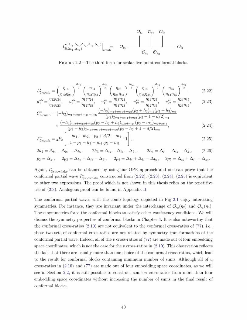
I∗(∆i3

,∆i4,∆i2

,∆i5,∆i1

)

5(∆k1,∆k2

)

∣∣∣comb

= Oi3 Oi1

Oi4 Oi2 Oi5

Ok1 Ok2

Figure 2.2 – The third form for scalar five-point conformal blocks.

L∗5|comb =

(η14

η12η24

)∆i22(

η24

η23η34

)∆i32(

η23

η24η34

)∆i42(

η14

η15η45

)∆i52(

η45

η14η15

)∆i12

, (2.22)

u∗51 =η12η34

η14η23, u∗52 =

η15η24

η12η45, v∗511 =

η13η24

η14η23, v∗512 =

η14η25

η12η45, v∗522 =

η24η35

η23η45, (2.23)

C∗5|comb = (−h2)m1+m2+m11+m22

(−h3)m1+m11+m22(p2 + h2)m1(p2 + h3)m1

(p2)2m1+m11+m22(p2 + 1− d/2)m1

× (−h4)m2+m12+m22(p3 − h2 + h4)m2+m11(p3 −m1)m2+m12

(p3 − h2)2m2+m11+m12+m22(p3 − h2 + 1− d/2)m2

, (2.24)

F ∗5|comb = 3F2

[−m1,−m2,−p2 + d/2−m1

1− p2 − h2 −m1, p3 −m1

; 1

], (2.25)

2h2 = ∆i2 −∆k2 −∆k1 , 2h3 = ∆i4 −∆i3 −∆k1 , 2h4 = ∆i1 −∆i5 −∆k2 , (2.26)

p2 = ∆k1 , 2p3 = ∆k2 + ∆i2 −∆k1 , 2p4 = ∆i3 + ∆i4 −∆k1 , 2p5 = ∆i5 + ∆i1 −∆k2 .

Again, I∗5|snowflake can be obtained by using our OPE approach and one can prove that theconformal partial wave I∗5|snowflake constructed from (2.22), (2.23), (2.24), (2.25) is equivalentto other two expressions. The proof which is not shown in this thesis relies on the repetitiveuse of (2.3). Analogous proof can be found in Appendix B.

The conformal partial waves with the comb topology depicted in Fig 2.1 enjoy interestingsymmetries. For instance, they are invariant under the interchange of Oi2(η2) and Oi3(η3).These symmetries force the conformal blocks to satisfy other consistency conditions. We willdiscuss the symmetry properties of conformal blocks in Chapter 4. It is also noteworthy thatthe conformal cross-ratios (2.10) are not equivalent to the conformal cross-ratios of (77), i.e.,these two sets of conformal cross-ratios are not related by symmetry transformations of theconformal partial wave. Indeed, all of the v cross-ratios of (77) are made out of four embeddingspace coordinates, which is not the case for the v cross-ratios in (2.10). This observation reflectsthe fact that there are usually more than one choice of the conformal cross-ratios, which leadto the result for conformal blocks containing minimum number of sums. Although all of ucross-ratios in (2.10) and (77) are made out of four embedding space coordinates, as we willsee in Section 2.2, it is still possible to construct some u cross-ratios from more than fourembedding space coordinates without increasing the number of sums in the final result ofconformal blocks.

40

I(∆i2

,...,∆i6,∆i1

)

6(∆k1,∆k2

,∆k3)

∣∣∣comb

= Oi2 Oi1

Oi3 Oi4 Oi5 Oi6

Ok1 Ok2 Ok3

I(∆i2

,...,∆i6,∆i1

)

6(∆k1,∆k2

,∆k3)

∣∣∣snowflake

= Ok1

Oi2

Oi3Ok2

Oi5Oi4

Ok3

Oi6

Oi1

Figure 2.3 – Scalar six-point conformal blocks with the comb (top) and snowflake (bottom)topology.

As we mentioned earlier, the OPE approach introduced in this thesis allows us to computeconformal blocks with any topology. In the following sections, this statement will be madeevident by using our OPE approach to compute six- and seven-point conformal blocks beyondthe comb topology.

2.2 Six-point conformal blocks with the snowflake topology

Besides the comb topology, six-point conformal blocks have another topology which can beobtained by OPE expanding the six external quasi-primary operators in pairs, see Fig 2.3. Bothtopologies for six-point conformal blocks can be obtained from five-point conformal blocks,depicted in Figure 2.2. Indeed, from Figure 2.2, it is clear that the external quasi-primaryoperator Oi2 is different. Transforming one of the external quasi-primary operators Oi1 , Oi3 ,Oi4 , or Oi5 into exchanged quasi-primary operators by appending two new external quasi-primary operators leads to the scalar six-point correlation function with the comb topology,while doing the same with the quasi-primary operator Oi2 gives instead the scalar six-pointcorrelation with the snowflake topology.

We start with five-point conformal blocks, add the OPE in the way mentioned above, andfollow the four steps in our OPE strategy, to get desired six-point conformal blocks with the

41

snowflake topology

L(∆i2

,...,∆i6,∆i1

)

6|snowflake =

(η13

η12η23

)∆i22(

η12

η13η23

)∆i32(

η35

η34η45

)∆i42

(2.27)

×(

η34

η35η45

)∆i52(

η15

η16η56

)∆i62(

η56

η15η16

)∆i12

,

u61 =

η15η23

η12η35, u6

2 =η13η45

η15η34, u6

3 =η16η35

η13η56,

v611 =

η13η25

η12η35, v6

12 =η14η35

η15η34, v6

22 =η13η24

η12η34, (2.28)

v613 =

η15η26

η12η56, v6

23 =η15η36

η13η56, v6

33 =η35η46

η34η56,

with

C(d,h;p)6|snowflake =

(p2 + h3)m1+m23(p3)−m1+m2+m3+m12+m33(−h3)m1+m11+m22+m13

(p2)2m1+m11+m13+m22+m23(p2 + 1− d/2)m1

(2.29)

× (p3 − h2 + h4)m2+m11(p2 + h2)m1−m2+m3+m13+m23(−h4)m2+m12+m22+m33

(p3 − h2)2m2+m11+m12+m22+m33(p3 − h2 + 1− d/2)m2

× (p3 + h2 + h5)m3+m12(−h2)m1+m2−m3+m11+m22(−h5)m3+m13+m23+m33

(p3 + h2)2m3+m12+m13+m23+m33(p3 + h2 + 1− d/2)m3

,

as well as

F(d,h;p)6|snowflake(m) =

(−p3 + h2 + d/2−m2)m2

(p3)−m1(−h2 +m1)−m3

∑t1,t2≥0

(−m1)t2(−m2)t1(−m3)t2(p3 − h2 + 1− d/2)t1

× (p3)t1(p3 − d/2)t1(−p2 + d/2−m1)t2(1 + h2 −m1 +m3)−t1(1 + h2 −m1)−t1+t2(p3 −m1)t1+t2t1!t2!

=(−p3 + h2 + d/2−m2)m2

(p3)−m1(−h2)−m3

(2.30)

× F 1,3,22,1,0

[p3 − d/2;−m2,−h2, p3;−m1,−m3

−h2 −m3, p3 −m1; p3 − h2 + 1− d/2;−

∣∣∣∣∣ 1, 1],

and finally

2h2 = ∆k3 −∆k2 −∆k1 , 2h3 = ∆i3 −∆i2 −∆k1 ,

2h4 = ∆i5 −∆i4 −∆k2 , 2h5 = ∆i1 −∆i6 −∆k3 ,

p2 = ∆k1 , 2p3 = ∆k2 + ∆k3 −∆k1 , 2p4 = ∆i2 + ∆i3 −∆k1 ,

2p5 = ∆i4 + ∆i5 −∆k2 , 2p6 = ∆i6 + ∆i1 −∆k3 .

The function F6|snowflake (2.30) in the snowflake configuration is also a double sum of thehypergeometric type, same as in the comb configuration. In contrast to F6|comb in (2.14) withM = 6 , the snowflake double sum does not factorize into two hypergeometric functions, Itcan however be written as a Kampé de Fériet function F 1,3,2

2,1,0 , defined as (114; 115)

F p,r,uq,s,v

[a; c;f

b;d; g

∣∣∣∣∣x, y]

=∑m,n≥0

(a)m+n(c)m(f)n(b)m+n(d)m(g)n

xmyn

m!n!, (2.31)

42

where

(a)m+n = (a1)m+n · · · (ap)m+n, (b)m+n = (b1)m+n · · · (bq)m+n,

(c)m = (c1)m · · · (cr)m, (d)m = (d1)m · · · (ds)m,

(f)n = (f1)n · · · (fu)n, (g)n = (g1)n · · · (gv)n.

2.2.1 An alternative form

Again, all of the u cross-ratios in (2.28) are made out of four embedding space coordinates. Inthis subsection, we provide an alternative form for six-point scalar conformal blocks with thesnowflake topology, in which all of the u cross-ratios contain six embedding space coordinates.We put this alternative form here without showing any computation. One can get the resultby using our OPE approach. In this alternative form, we choose the legs L∗6|snowflake and theconformal cross-ratios as

L∗6|snowflake =

(η13

η12η23

)∆i22(

η12

η13η23

)∆i32(

η15

η14η45

)∆i42

(2.32)

×(

η14

η15η45

)∆i52(

η12

η16η26

)∆i62(

η26

η12η16

)∆i12

,

and

u∗61 =η23η15η34

η13η24η35, u∗62 =

η12η34η45

η14η35η24, u∗63 =

η16η24η35

η26η15η34,

v∗611 =η12η34

η13η24, v∗612 =

η34η25

η24η35, v∗613 =

η12η36

η13η26, (2.33)

v∗622 =η15η34

η14η35, v∗623 =

η12η46

η14η26, v∗633 =

η12η56

η15η26,

respectively. The resulting scalar six-point conformal blocks with the snowflake topology are

C∗6 =(p3 − h2 + h4)m2+m12+m33

(−h2)m1+m2−m3+m12

(−h3)m1+m12(p3)−m1+m2+m3+m23+m33(p2 + h3)m1+m11+m13

(p2)2m1+m11+m12+m13(p2 + 1− d/2)m1

× (p3 − h2 + h4)m2+m12+m33(p2 + h2)m1−m2+m3+m13(−h4)m2+m22+m23

(p3 − h2)2m2+m12+m22+m23+m33(p3 − h2 + 1− d/2)m2

(2.34)

× (p3 + h2 + h5)m3(−h2)m1+m2−m3+m12+m22(−h5)m3+m13+m23+m33

(p3 + h2)2m3+m13+m23+m33(p3 + h2 + 1− d/2)m3

,

with F ∗6|snowflake = F6|snowflake, given by (2.30).

We note here that although the alternative forms for u cross-ratios are made out of six embed-ding space coordinates, F ∗6|snowflake and F6|snowflake are the same function, which implies thatG∗6|snowflake and G6|snowflake contain the same number of sums. From all of the results that wehave up to now, it seems that there is a vast number of possibilities to choose the conformalcross-ratios. Perhaps, demanding that the conformal cross-rations have proper behaviours un-der the OPE limits and that the result for conformal blocks contain minimum number of sums

43

are only constraints that we can ask for the conformal cross-ratios. Conformal cross-ratiostransforming properly under the OPE limits are easy to build, while finding a set of conformalcross-ratios that lead to a simple result for the conformal block is practically hard.

It is noteworthy that although different legs, conformal cross-ratios, C-functions are chosen,the two results for six-point conformal partial wave with the snowflake topology must beequivalent. We will analytically prove the equivalence between the two results in Appendix B.

In Sections 2.1.1 and 2.1.2, we checked the unit operator and OPE limit for scalar M -pointconformal blocks with the comb topology. The behaviour of the scalar six-point conformalblocks with the snowflake topology in these two types of limit can also be verified, to whichwe now turn.

2.2.2 Limit of Unit Operator

Naively, the limit of unit operator should be verified for all of the six external quasi-primaryoperators. However, the symmetry properties of I6|snowflake, which will be discussed in Chapter4, allow us to verify the limit of unit operator for just one quasi-primary operator. We choosethis quasi-primary operator to be Oi6(η6)→ 1, for which ∆i6 = 0, ∆k3 = ∆i1 , and

I(∆i2

,∆i3,∆i4

,∆i5,∆i6

,∆i1)

6(∆k1,∆k2

,∆k3)

∣∣∣snowflake

→ I(∆i2

,∆i3,∆i1

,∆i4,∆i5

)

5(∆k1,∆k2

)

∣∣∣comb

. (2.35)

To proceed, we start with the six-point conformal partial wave (2.27), (2.28), (2.29), and (2.30)and choose I∗5|snowflake constructed from (2.22), (2.23), (2.24), (2.25) as the representative ofscalar five-point conformal partial wave. Since h5 = p6 = 0 and the remaining vector elementsof h and p translate directly into their five-point counterparts (2.26) in the limit of unitoperator Oi6(η6) → 1, the sums over m3, m13, m23, and m33 in (2.29) are trivial due to thePochhammer symbol (−h5)m3+m13+m23+m33 , forcing m3 = m13 = m23 = m33 = 0. Therefore,the conformal cross-ratios u6

3, v613, v6

23, and v633 disappear in the limit.

The remaining conformal cross-ratios (2.28) relate to the conformal cross-ratios (2.24) as in

u6a → u∗5a (1 ≤ a ≤ 2), v6

ab → v∗5ab (1 ≤ a ≤ b ≤ 2), (2.36)

and thus

L6

∏1≤a≤3

(u6a)

∆ka2 → L∗5

∏1≤a≤2

(u∗5a )∆ka

2 . (2.37)

These observations imply that G6 → G∗5 in the limit of unit operator, which is straightforwardto verify since m3 = m13 = m23 = m33 = 0.

2.2.3 OPE Limit

For scalar six-point correlation functions with the snowflake topology depicted in Figure 2.3,the possible OPE limits are η2 → η3, η4 → η5, and η6 → η1. However, combining with the

44

rotation symmetries of the six-point conformal partial wave I6|snowflake, it is only necessary toverify the behaviour of I6|snowflake in one OPE limit. Here, we explicitly check that in the limitη2 → η3, we have

I(∆i2

,∆i3,∆i4

,∆i5,∆i6

,∆i1)

6(∆k1,∆k2

,∆k3)

∣∣∣snowflake

→ 1

η12

(∆2+∆3−∆k1)

23

I(∆i5

,∆i4,∆i3

,∆i6,∆i1

)

5(∆k2,∆k3

)

∣∣∣comb

. (2.38)

For this proof, we start from the alternative form of the scalar six-point conformal partial wavewith the snowflake topology given in Section 2.2.1, which must reduce to the scalar five-pointconformal partial wave I5|comb with the comb topology in the OPE limit (2.38). We choose theresult of (77) (see also Appendix A) as the representation for the scalar five-point conformalpartial wave I5|comb. This choice is of no consequence since the different representations of thesame conformal partial wave are equivalent, see Appendices A and B.

In the OPE limit (2.38), the legs L∗6|snowflake (2.32) and the conformal cross-ratios (2.33)transform as

L∗6∏

1≤a≤3

(u∗6a )∆ka

2 → 1

(η23)12

(∆2+∆3−∆k1)(vP34)h5LP5

∏1≤a≤2

(uPa )∆ka

2 ,

u∗61 → 0, u∗62 → uP1 , u∗63 →uP2vP34

,

v∗61a → 1 (1 ≤ a ≤ 3),

v∗622 → vP23, v∗623 →vP24

vP34

, v∗633 →1

vP34

,

where uPa and vPab are the conformal cross-ratios used in (77), and the conformal dimensionson the RHS are the ones relevant for the five-point correlation functions, i.e.

p3 − h2 + h4 → p3, p3 → p3 + h3, p2 + h2 → p4, h5 → h4, h2 → h3,

p3 + h2 + h5 → p4 + h4, p3 + h2 → p4 + h3, h4 → −p2 − h2, p3 − h2 → p3 + h2.

Thus, the OPE limit (2.38) translates into the identity

(vP34)h5G∗6 = GP5 ,

with the appropriate changes for the vectors h and p.

Since F ∗6|snowflake transforms as

F ∗6 = F6 →(p2 + h2 −m2)m2

(−h2)−m3

3F2

[−m2,−m3, p3 − d/2

p2 + h2 −m2,−h2 −m3

; 1

]=

(p2 + h2 −m2)m2

(−h2)−m3

FP5 ,

45

in the OPE limit (2.38), we have

(vP34)h5G∗6 =∑ (p3)m2+m3+m23+m33(−h2 −m3)m2+m22(−h5)m3+m23+m33(p3 + h2 + h5)m3

(p3 + h2)2m3+m23+m33(p3 + h2 + 1− d/2)m3

× (p2 + h2 −m2)m3(−h4)m2+m22+m23(p3 − h2 + h4)m2+m33

(p3 − h2)2m2+m22+m23+m33(p3 − h2 + 1− d/2)m2

(m23

k23

)(m33

k33

)×(k23

m′24

)(h5 −m3 − k23 − k33

m′34

)(−1)k23+k33+m′24+m′34

× (uP1 )m2

m2!

(uP2 )m3

m3!

(1− vP23)m22

m22!

(1− vP24)m′24

m23!

(1− vP34)m′34

m33!FP5 ,

after expanding in the proper conformal cross-ratios uPa and (1−vPab) of (77). Here the vectorsh and p are still the original ones. Thus to complete the proof, we need to evaluate the extrasums for which we did not explicitly write the indices of summation (to make the notation lesscluttered) with the help of (2.3), and express the vectors h and p in terms of the five-pointones.

First, we compute the sum over k22 and then k23 after changing the variable by k23 → k23+m′24,which lead to

(vP34)h5G∗6 =∑ (p3)m2+m3+m23+m33(−h2 −m3)m2+m22(−h5)m3+m′24+m′34

(p3 + h2 + h5)m3

(p3 + h2)2m3+m23+m33(p3 + h2 + 1− d/2)m3

× (p2 + h2 −m2)m3(−h4)m2+m22+m23(p3 − h2 + h4)m2+m33

(p3 − h2)2m2+m22+m23+m33(p3 − h2 + 1− d/2)m2

(−m′34)m23+m33−m′24

m33!(m23 −m′24)!

× (uP1 )m2

m2!

(uP2 )m3

m3!

(1− vP23)m22

m22!

(1− vP24)m′24

m′24!

(1− vP34)m′34

m′34!FP5 .

We then shift m23 by m23 → m23 + m′24, and then redefine m33 = m − m23. With thesechanges, we can compute the sums over m23 and then m, which give

(vP34)h5G∗6 =∑ (p3)m2+m3+m′24

(−h2)m2−m3+m22(−h5)m3+m′24+m′34(p3 + h2 + h5)m3

(−h2)−m3(p3 + h2)2m3+m′24+m′34(p3 + h2 + 1− d/2)m3

×(p2 + h2)−m2+m3+m′34

(−h4)m2+m22+m′24(p3 − h2 + h4)m2

(p2 + h2)−m2(p3 − h2)2m2+m22+m′24(p3 − h2 + 1− d/2)m2

× (uP1 )m2

m2!

(uP2 )m3

m3!

(1− vP23)m22

m22!

(1− vP24)m′24

m′24!

(1− vP34)m′34

m′34!FP5 .

Finally, changing the vectors h and p by their five-point counterparts and renamingm2 → m1,m3 → m1, m22 → m23, m′24 → m24, and m′34 → m34, we have

FP5 = 3F2

[−m2,−m3, p3 − d/2

p2 + h2 −m2,−h2 −m3

; 1

]→ 3F2

[−m1,−m2, p4 + h2 − d/2

p4 −m1,−h3 −m2

; 1

],

which indeed proves that (vP34)h5G∗6 = GP5 , as expected.

The six-point conformal blocks with the snowflake topology derived in this section give thefirst example of higher-point conformal blocks beyond the comb topology. In principle, with

46

the embedding space OPE approach, explicit results for any higher-point conformal partialwave of interest can be obtained, after straightforward (yet somewhat tedious) re-summationsof the hypergeometric type (2.3) and (2.4). We note that properly taking the OPE limit or thelimit of unit operator for the scalar six-point conformal partial waves with scalar exchangesin the snowflake configuration, which can be obtained by doubling the external legs of three-point correlation functions once, we can reach all scalar M < 6-point conformal partial waveswith scalar exchanges irrespective of topologies. This observation can be generalized to scalar(3 × 2N )-point conformal partial waves with scalar exchanges, which can be obtained bydoubling the number of all external legs of three-point correlation functions N times. Fromthe successive action of the OPE limit or the limit of unit operator, these (3 × 2N )-pointconformal partial waves should lead to all topologies for smaller scalar higher-point conformalpartial waves with scalar exchanges (starting from sufficiently large N). This statement canbe further generalized. Since all of M > 3-point conformal partial waves lead to three-pointcorrelation functions after successively taking the OPE limit, (3×2N )-point conformal partialwaves can be obtained from (M × 2N )-point conformal partial waves by properly taking theOPE limit. We thus conclude that from the successive action of the OPE limit or the limit ofunit operator, scalar (M×2N )-point conformal partial waves with scalar exchanges should leadto all topologies for smaller scalar higher-point conformal partial waves with scalar exchanges(starting from sufficiently large N).

The whole discussion here provides a systematical way to compute any scalar higher-pointconformal block with scalar exchanges. One first compute a specific class of (M × 2N )-pointconformal partial waves for any N , for example (3×2N )-point conformal partial waves mentio-ned above. Then successively taking the OPE limit leads to desired results. Although this wayis systematical, it is practically hard due to the necessity of (M × 2N )-point conformal partialwaves. Moreover, one can not directly write down an explicit result for any scalar higher-pointconformal block even with the knowledge of (M × 2N )-point conformal partial waves. TheOPE limit must be performed, leading to superfluous sums which must be re-summed.

A more practical and efficient way to compute any scalar higher-point conformal block withscalar exchanges is to use Feynman-like rules. Before going to discuss such rules, we computethe scalar seven-point conformal partial waves with scalar exchanges in the extended snowflakeconfiguration, which combining with the previous results for M -point conformal partial waveswith the comb topology and six-point conformal partial waves with the snowflake topology,suggest the existence of Feynman-like rules for scalar higher-point conformal blocks with scalarexchanges.

47

I(∆i2

,...,∆i7,∆i1

)

7(∆k1,∆k2

,∆k3,∆k4

)

∣∣∣extendedsnowflake

= Ok2

Oi3

Oi4Ok3

Oi6Oi5

Ok1

Oi2

Ok4

Oi7

Oi1

Figure 2.4 – The seven-point conformal blocks with the extended snowflake topology.

2.3 Seven-point conformal blocks with the extended snowflaketopology

As for six-point conformal blocks, there are two different topologies for seven-point confor-mal blocks, dubbed the comb topology discussed before and the extended snowflake channelillustrated in Figure 2.4. The scalar seven-point conformal blocks with scalar exchanges in theextended snowflake configuration can be computed from the scalar six-point conformal partialwaves with both topologies discussed in Section 2.2.

Starting from six-point conformal partial waves with the comb topology, obtaining seven-pointconformal partial waves with the extended snowflake topology necessitate the action of theOPE on one of the two quasi-primary operators inside the comb, i.e. on Oi4 or Oi5 in Figure3.4. Acting on any one of the other quasi-primary operators leads to the seven-point conformalpartial waves with the comb topology. On the contrary, due to the symmetry properties ofthe six-point snowflake conformal partial waves seen in Figure 2.3, the OPE can be performedanywhere on the snowflake topology to get the extended snowflake topology.

Following the OPE strategy mentioned in the beginning of this chapter, we start from the scalarsix-point conformal blocks with scalar exchanges in the snowflake configuration (2.27), (2.28),(2.29) and (2.30). To proceed, we redefine the quasi-primary operators such that Oia(ηa) →Oia−1(ηa−1) with the knowledge that Oi0(η0) ≡ Oi6(η6), and finally apply (2.2) with k = 5,l = 6 and m = 6. After choosing the legs factor as

L7|extendedsnowflake

=

(η16

η12η26

)∆i22(

η24

η23η34

)∆i32(

η23

η24η34

)∆i42

(2.39)

×(

η46

η45η56

)∆i52(

η45

η46η56

)∆i62(

η16

η17η67

)∆i72(

η67

η16η17

)∆i12

,

48

and the conformal cross-ratios as

u71 =

η12η46

η16η24, u7

2 =η26η34

η23η46, u7

3 =η24η56

η26η45, u7

4 =η17η26

η12η67, (2.40)

v711 =

η14η26

η16η24, v7

12 =η24η36

η23η46, v7

13 =η15η46

η16η45, v7

14 =η16η27

η12η67, (2.41)

v722 =

η13η26

η16η23, v7

23 =η25η46

η26η45, v7

24 =η26η37

η23η67, v7

33 =η24η35

η23η45,

v734 =

η26η47

η24η67, v7

44 =η46η57

η45η67,

the resulting C7|extendedsnowflake

and F7|extendedsnowflake

are given by

C(d,h;p)

7|extendedsnowflake(m,m) (2.42)

=(p2 + h3)m1−m4+m23(p3)−m1+m2+m3+m12+m33(−h3)m1+m4+m11+m13+m22+m24+m34+m44

(p2)2m1+m11+m13+m22+m23+m24+m34+m44(p2 + 1− d/2)m1

× (p3 − h2 + h4)m2+m11+m34(p2 + h2)m1−m2+m3+m13+m23+m44(−h4)m2+m12+m22+m24+m33

(p3 − h2)2m2+m11+m12+m22+m24+m33+m34(p3 − h2 + 1− d/2)m2

× (p3 + h2 + h5)m3+m12(−h2)m1+m2−m3+m11+m22+m24+m34(−h5)m3+m13+m23+m33+m44

(p3 + h2)2m3+m12+m13+m23+m33+m44(p3 + h2 + 1− d/2)m3

× (p4 −m1)m4+m14(−h6)m4+m14+m24+m34+m44(p4 − h3 + h6)m4+m11+m13+m22

(p2 + h3 +m1)−m4(p4 − h3)2m4+m11+m13+m14+m22+m24+m34+m44(p4 − h3 + 1− d/2)m4

,

and

F(d,h;p)

7|extendedsnowflake(m) =

1

(p3)−m1(−p3 + h2 + d/2)−m2(−p3 − h2 + d/2)−m3

× F 2,1,11,1,1

[p3 − d/2, p3;−m2;−m3

p3 −m1; p3 − h2 + 1− d/2; p3 + h2 + 1− d/2

∣∣∣∣∣ 1, 1]

× 3F2

[−m1,−m4,−p2 + d/2−m1

p4 −m1, 1− p2 − h3 −m1

; 1

], (2.43)

respectively. In (2.42), h and p are again functions of conformal dimensions of both externaland internal quasi-primary operators,

2h2 = ∆k3 −∆k2 −∆k1 , 2h3 = ∆i2 −∆k4 −∆k1 , 2h4 = ∆i4 −∆i3 −∆k2 ,

2h5 = ∆i6 −∆i5 −∆k3 , 2h6 = ∆i1 −∆i7 −∆k4 , (2.44)

p2 = ∆k1 , 2p3 = ∆k2 + ∆k3 −∆k1 , 2p4 = ∆k4 + ∆i2 −∆k1 ,

2p5 = ∆i3 + ∆i4 −∆k2 , 2p6 = ∆i5 + ∆i6 −∆k3 , 2p7 = ∆i7 + ∆i1 −∆k4 .

It is noteworthy that F7|extendedsnowflake

in (2.43) can be written as a product of F6|snowflake andF5|comb, i.e.

F7|extendedsnowflake

= F6|snowflakeF5|comb, (2.45)

49

This factorization is reminiscent of the factorization seen in the comb configuration (2.14). Be-fore discussing this interesting factorization, we first verify that the scalar seven-point confor-mal blocks with the extended snowflake topology exhibit the proper behaviour under the OPElimit and the limit of unit operator. All proofs are left for Appendixes C and D.

2.3.1 Limit of Unit Operator

For scalar seven-point conformal partial waves with scalar exchanges in the extended snowflakeconfiguration, depicted in Fig 2.4, combining with the symmetry properties, there are onlythree limits of unit operator to check. They are Oi2(η2)→ 1, Oi3(η3)→ 1 and Oi7(η7)→ 1,respectively.

Focusing first on the limit Oi7(η7)→ 1, we have ∆i7 = 0, ∆k4 = ∆i1 , and

I(∆i2

,∆i3,∆i4

,∆i5,∆i6

,∆i7,∆i1

)

7(∆k1,∆k2

,∆k3,∆k4

)

∣∣∣extendedsnowflake

→Oi7 (η7)→1

I(∆i1

,∆i2,∆i3

,∆i4,∆i5

,∆i6)

6(∆k1,∆k2

,∆k3)

∣∣∣snowflake

.

In this limit, it is straightforward to see that h6 = p7 = 0. Moreover, the remaining compo-nents of the vectors h and p (2.44) become the appropriate components of the scalar six-pointconformal partial waves with the snowflake topology. Since the conformal cross-ratios trans-form as

u7a → u6

a (1 ≤ a ≤ 3), v7ab → v6

ab, (1 ≤ a ≤ b ≤ 3),

and the remaining conformal cross-ratios disappear due to the sums over m4, m14, m24, m34

and m44 in (2.42) being trivial due to the Pochhammer symbol (−h6)m4+m14+m24+m34+m44

forcing m4 = m14 = m24 = m34 = m44 = 0, we obtain

L7|extendedsnowflake

∏1≤a≤3

(u7a)

∆ka2 → L6|snowflake

∏1≤a≤3

(u6a)

∆ka2 ,

with the appropriate topology.

Furthermore, the limit of unit operator Oi7(η7)→ 1 leads to

F7|Oi7→1 =(−p3 − h2 + d/2−m3)m3(−p3 + h2 + d/2−m2)m2

(p3)−m1

∑r1,r2≥0

(−m2)t1(−m3)t2t1!t2!

× (p3 − d/2)t1+t2

(p3 + h2 + 1− d/2)t2(p3 −m1)t1+t2

(p3)t1+t2

(p3 − h2 + 1− d/2)t1,

which implies F7|extendedsnowflake

→ F6snowflake with the help of the standard 3F2-hypergeometric

function identity (2.4). Taking into account that C7|extendedsnowflake

→ C6|snowflake trivially, we thus

prove that G7|extendedsnowflake

→ G6|snowflake in the limit of unit operator Oi7(η7)→ 1.

The two remaining limits of unit operator being longer, their proofs are left for Appendix C.

50

2.3.2 OPE Limit

For scalar seven-point conformal partial waves with the extended snowflake topology, as de-picted in Figure 2.4, there are only two possible OPE limits, thanks to the symmetry groupof I

7|extendedsnowflake. They are η3 → η4 and η7 → η1, respectively.

For the limit η7 → η1, we have

I(∆i2

,∆i3,∆i4

,∆i5,∆i6

,∆i7,∆i1

)

7(∆k1,∆k2

,∆k3,∆k4

)

∣∣∣extendedsnowflake

→η7→η1

(η17)−p7 I(∆i2

,∆i3,∆i4

,∆i5,∆i6

,∆i1)

6(∆k1,∆k2

,∆k3)

∣∣∣snowflake

, (2.46)

as well as

L7

∏1≤a≤4

(u7a)

∆ka2 → (η17)−p7L6

∏1≤a≤3

(u6a)

∆ka2 ,

u71 → u6

1, u72 → u6

2, u73 → u6

3, u74 → 0,

v711 → v6

11, v712 → v6

12, v713 → v6

13, v714 → 1,

v722 → v6

22, v723 → v6

23, v724 → v6

22, v733 → v6

33,

v734 → v6

11, v744 → v6

13.

Here, the quantities and the conformal dimensions on the RHS of the limits are the onesrelevant for the six-point conformal partial waves with the snowflake topology, i.e. (2.27),(2.28), (2.29), (2.30) and trivial substitutions for the vectors h and p.

As a consequence, the OPE limit η7 → η1 leads to the identity G7|η7→η1= G6, or more

precisely

G(d,h2,h3,h4,h5,h6;p2,p3,p4,p5,p6,p7)

7|extendedsnowflake(u6

1, u62, u

63, 0; v6

11, v612, v

613, 1, v

622, v

623, v

622, v

633, v

611, v

613)

= G(d,h2,h3,h4,h5;p2,p3,p4,p5,p6)6|snowflake (u6

1, u62, u

63; v6

11, v612, v

613, v

622, v

623, v

633).

Since F7 → F6 in that limit, we have

G7|η7→η1=

∑ma,mab≥0

(p2 + h3)m1+m23(p3)−m1+m2+m3+m12+m33(−h3)m1+m11+m13+m22

(p2)2m1+m11+m13+m22+m23(p2 + 1− d/2)m1

× (p3 − h2 + h4)m2+m11(p2 + h2)m1−m2+m3+m13+m23(−h4)m2+m12+m22+m33

(p3 − h2)2m2+m11+m12+m22+m33(p3 − h2 + 1− d/2)m2

× (p3 + h2 + h5)m3+m12(−h2)m1+m2−m3+m11+m22(−h5)m3+m13+m23+m33

(p3 + h2)2m3+m12+m13+m23+m33(p3 + h2 + 1− d/2)m3

× (−h6)m24+m34+m44(p4 − h3 + h6)m11+m13+m22−m24−m34−m44

(p4 − h3)m11+m13+m22

× F6m11!m13!m22!

(m11 −m34)!(m13 −m44)!(m22 −m24)!m24!m34!m44!

×∏

1≤a≤3

(u6a)ma

ma!

∏1≤a≤b≤3

(1− v6ab)

mab

mab!,

51

where we performed the following change of variables,

m11 → m11 −m34, m13 → m13 −m44, m22 → m22 −m24.

Evaluating the sums overm24,m34, and finallym44 using standard hypergeometric re-summationformula straightforwardly leads to G7|η7→η1

= G6, proving (2.46).

Since the proof for the last independent OPE limit η3 → η4 is more intricate, it is left forAppendix D.

2.4 Feynman-like rules

The factorization of F7|extendedsnowflake

(2.45) and FM |comb (2.14) seems to suggest that there existsome Feynman-like rules for any scalar higher-point conformal partial waves with scalar ex-changes. In this section we will discuss the existence of such rules by looking at the results forhigher-point conformal partial waves obtained in this chapter.

First, after rewriting the vectors h and p explicitly in terms of the conformal dimensions in theknown C-functions including the C-function (2.11) for the scalar M -point conformal blockswith the comb topology, the C-function (2.29) for the scalar six-point conformal blocks withthe snowflake topology as well as the C-function (2.42) for the seven-point conformal blockswith the extended snowflake topology, it is clear that a pattern emerges. Indeed, in terms ofthe conformal dimensions, these C-functions are given by

C(d,h;p)M |comb(m,m) =

(∆k1−∆i2

+∆i32

)m1+tr1m

(∆k1

+∆i2−∆i3

2

)m1+tr0m

(∆k1)2m1+m1+ ¯m1(∆k1 + 1− d/2)m1

×

(∆kM−3

−∆i1+∆iM

2

)mM−3+mM−4

(∆kM−3

+∆i1−∆iM

2

)mM−3+mM−3+ ¯mM−3

(∆kM−3)2mM−3+mM−4+mM−3+ ¯mM−3

(∆kM−3+ 1− d/2)mM−3

×

(∆k2−∆k1

+∆i42

)m2−m1+tr2m

(∆k2

+∆k1−∆i4

2

)m2+m1+m1+ ¯m1

(∆k2)2m2+m1+m2+ ¯m2(∆k2 + 1− d/2)m2

×

(∆i4−∆k2

+∆k12

)m1

(∆i4−∆k2

+∆k12

)m1−m2(

∆i4+∆k2

−∆k12

)−m1

(∆i4−∆k2

+∆k12

)m1−m2

×

(∆k3−∆k2

+∆i52

)m3−m2+tr3m

(∆k3

+∆k2−∆i5

2

)m3+m2+m2+ ¯m2

(∆k3)2m3+m2+m3+ ¯m3(∆k3 + 1− d/2)m3

×

(∆i5−∆k3

+∆k22

)m2

(∆i5−∆k3

+∆k22

)m2−m3+m1(

∆i5+∆k3

−∆k22

)−m2

(∆i5−∆k3

+∆k22

)m2−m3

...

52

as well as

C(d,h;p)6|snowflake(m,m) =

(∆k1−∆i2

+∆i32

)m1+m23

(∆k1

+∆i2−∆i3

2

)m1+m11+m22+m13

(∆k1)2m1+m11+m13+m22+m23(∆k1 + 1− d/2)m1

×

(∆k2−∆i4

+∆i52

)m2+m11

(∆k2

+∆i4−∆i5

2

)m2+m12+m22+m33

(∆k2)2m2+m11+m12+m22+m33(∆k2 + 1− d/2)m2

×

(∆k3−∆i6

+∆i12

)m3+m12

(∆k3

+∆i6−∆i1

2

)m3+m13+m23+m33

(∆k3)2m3+m12+m13+m23+m33(∆k3 + 1− d/2)m3

×(−∆k1 + ∆k2 + ∆k3

2

)−m1+m2+m3+m12+m33

×(−∆k2 + ∆k3 + ∆k1

2

)−m2+m3+m1+m13+m23

×(−∆k3 + ∆k1 + ∆k2

2

)−m3+m1+m2+m11+m22

,

and

C(d,h;p)

7|extendedsnowflake(m,m) =

(∆k2−∆i3

+∆i42

)m2+m11+m34

(∆k2

+∆i3−∆i4

2

)m2+m12+m22+m24+m33

(∆k2)2m2+m11+m12+m22+m24+m33+m34(∆k2 + 1− d/2)m2

×

(∆k3−∆i5

+∆i62

)m3+m12

(∆k3

+∆i5−∆i6

2

)m3+m13+m23+m33+m44

(∆k3)2m3+m12+m13+m23+m33+m44(∆k3 + 1− d/2)m3

×

(∆k4−∆i7

+∆i12

)m4+m11+m13+m22

(∆k4

+∆i7−∆i1

2

)m4+m14+m24+m34+m44

(∆k4)2m4+m11+m13+m14+m22+m24+m34+m44(∆k4 + 1− d/2)m4

×

(∆k1−∆k4

+∆i22

)m1−m4+m23

(∆k1

+∆k4−∆i2

2

)m1+m4+m11+m13+m22+m24+m34+m44

(∆k1)2m1+m11+m13+m22+m23+m24+m34+m44(∆k1 + 1− d/2)m1

×

(∆i2

+∆k1−∆k4

2

)m1

(∆i2−∆k1

+∆k42

)−m1+m4+m14(

∆i2−∆k1

+∆k42

)−m1

(∆i2

+∆k1−∆k4

2

)m1−m4

×(−∆k1 + ∆k2 + ∆k3

2

)−m1+m2+m3+m12+m33

×(−∆k2 + ∆k3 + ∆k1

2

)−m2+m3+m1+m13+m23+m44

×(−∆k3 + ∆k1 + ∆k2

2

)−m3+m1+m2+m11+m22+m24+m34

,

respectively. The above C-functions hint that the hypothetical rules can be associated withdifferent vertices. Specifically, for each vertex constituting of two external quasi-primary ope-rators Oi and Oj as well as one internal quasi-primary operator Oka , the factor(

∆ka−∆i+∆j

2

)ma+...

(∆ka+∆i−∆j

2

)ma+...

(∆ka)2ma+...(∆ka + 1− d/2)ma, (2.47)

53

can be assigned, while for each vertex constituting of three internal quasi-primary operatorsOka , Okb , and Okc , the factor(

−∆ka + ∆kb + ∆kc

2

)−ma+mb+mc+...

(−∆kb + ∆kc + ∆ka

2

)−mb+mc+ma+...

(2.48)

×(−∆kc + ∆ka + ∆kb

2

)−mc+ma+mb+...

,

can be assigned.

It is reasonable to expect that a proper factor can be associate with each vertex constitutingof one external quasi-primary operator Oi and two internal quasi-primary operators Oka andOkb . By looking at the C-function for M -point comb conformal blocks, one can read off thisfactor as(

∆kb−∆ka+∆i

2

)mb−ma+...

(∆kb

+∆ka−∆i

2

)mb+ma+...

(∆kb)2mb+...(∆kb + 1− d/2)mb

(∆i−∆kb

+∆ka

2

)ma

(∆i−∆kb

+∆ka

2

)ma−mb+...(

∆i+∆kb−∆ka

2

)−ma

(∆i−∆kb

+∆ka

2

)ma−mb

.

(2.49)

However, it is easy to check that the second factor in the rule (2.49) does not work for theseven-point conformal blocks with the extended snowflake topology. Moreover, it is still unclearwhat the rules, which can be used to determine the dependence on the matrix of indices m(denoted by ellipses in the rules above), are. For a proper choice of v conformal cross-ratios,we conjecture that the remaining ambiguities can be fixed by the OPE limit and the limit ofunit operator and the Feynman-like rules of the C-function are dependent on choice of theconformal cross-ratios.

From the above discussion, it seems that the Feynman-like rules are associated with differentvertices, which can be classified by the number of internal quasi-primary operators. To verifythis statement further, we now turn to study the F -functions. As we mentioned earlier, theF -functions (2.14), (2.30), and (2.43), when expressed in terms of the conformal dimensions

F(d,h;p)M |comb(m) = 3F2

[−m1,−m2,−∆k1 + d/2−m1

∆k2−∆k1

+∆i42 −m1,

∆k2−∆k1

−∆i42 + 1−m1

; 1

]

× 3F2

[−m2,−m3,−∆k2 + d/2−m2

∆k3−∆k2

+∆i52 −m2,

∆k3−∆k2

−∆i52 + 1−m2

; 1

]...

× 3F2

[−mM−4,−mM−3,−∆kM−4

+ d/2−mM−4∆kM−3

−∆kM−4+∆iM−1

2 −mM−4,∆kM−3

−∆kM−4−∆iM−1

2 + 1−mM−4

; 1

]

54

as well as

F(d,h;p)6|snowflake(m) =

1(−∆k1

+∆k2+∆k3

2

)−m1

(−∆k2 + d/2)−m2(−∆k3 + d/2)−m3

× F 2,1,11,1,1

[∆k1

+∆k2+∆k3

−d2 ,

−∆k1+∆k2

+∆k32 ;−m2;−m3

−∆k1+∆k2

+∆k32 −m1; ∆k2 + 1− d/2; ∆k3 + 1− d/2

∣∣∣∣∣ 1, 1],

and finally

F(d,h;p)

7|extendedsnowflake(m) =

1(−∆k1

+∆k2+∆k3

2

)−m1

(−∆k2 + d/2)−m2(−∆k3 + d/2)−m3

× F 2,1,11,1,1

[∆k1

+∆k2+∆k3

−d2 ,

−∆k1+∆k2

+∆k32 ;−m2;−m3

−∆k1+∆k2

+∆k32 −m1; ∆k2 + 1− d/2; ∆k3 + 1− d/2

∣∣∣∣∣ 1, 1]

× 3F2

[−m1,−m4,−∆k1 + d/2−m1

∆k4−∆k1

+∆i22 −m1,

∆k4−∆k1

−∆i22 + 1−m1

; 1

],

satisfy interesting factorization properties, which strongly suggests that the hypothetical rulescan be associated with vertices. Indeed, the F -function forM -point conformal blocks with thecomb topology can be re-constructed if we associate the generalized hypergeometric function

F5|comb = 3F2

[−ma,−mb,−∆ka + d/2−ma

∆kb−∆ka+∆i

2 −ma,∆kb−∆ka−∆i

2 + 1−ma

; 1

],

to each vertex containing one external quasi-primary operator Oi and two internal quasi-primary operators Oka and Oka . The FM |comb (2.14) then can be obtained by multiplyingthese generalized hypergeometric functions together.

For the snowflake channel, a new type of vertex, which contains three internal quasi-primaryoperators, appears. As a result, another rules must be specified. From the known F6|snowflake

(2.30), it is natural to assign a factor

F6|snowflake =1(−∆ka+∆kb

+∆kc

2

)−ma

(−∆kb + d/2)−mb(−∆kc + d/2)−mc

× F 2,1,11,1,1

[∆ka+∆kb

+∆kc−d2 ,

−∆ka+∆kb+∆kc

2 ;−mb;−mc−∆ka+∆kb

+∆kc

2 −m1; ∆kb + 1− d/2; ∆kc + 1− d/2

∣∣∣∣∣ 1, 1],

to each vertex containing three internal quasi-primary operators.

The last type of vertex contains two external quasi-primary operators and one internal quasi-primary operator. The F -function factors for this type of vertex are

F4|comb = 1,

which can be easily read off from the four-point conformal blocks.

55

Figure 2.5 – One specific topology appearing in ten-point correlation functions.

We conjecture that the F -function for any conformal block can be built from F5|comb, F6|snowflake,and F4|comb, since anyM ≥ 4-point conformal block can be obtained by gluing the above threetypes of vertices. For example, for the ten-point conformal blocks, depicted in Fig 2.5, we ex-pect that the F10|topology of Figure 2.5 is given by

F10|topology of Figure 2.5 = (F5|combF6|snowflake)2,

where the proper parameters are determined by the quasi-primary operators as in (2.14) and(2.30). In general, the hypothetical rules for the F -function imply that the F -function for anyconformal block is given by

FM |any topology = (F5|comb)M−4−2n(F6|snowflake)n, (2.50)

where n is the number of vertices containing three internal quasi-primary operators and satis-fies 0 ≤ n ≤ bM−4

2 c.

We stress that although the hypothetical rules for the F -function apparently works for thescalar conformal blocks with scalar exchanges computed in this chapter, a rigorous proof is stillmissing. Moreover, to obtain the desired rules, we decompose the M -point conformal blocksinto a set of vertices. One can also work in the opposite way and reconstruct the possibletopologies by gluing the vertices. Indeed, if we denote the number of M -point conformalblocks, which contain n vertices that are made out of three internal quasi-primary operators,by T0(M ;n), then the gluing procedure implies that T0(M), which represents the number ofinequivalent topologies for M -point conformal blocks, should be expressible as

T0(M) =

bM−42c∑

n≥0

T0(M ;n). (2.51)

In summary, the discussion in this section suggests the existence of Feynman-like rules forscalar higher-point conformal blocks with scalar exchanges. The rules for the C-functions areincomplete which we conjecture can be fixed by the OPE limit and limit of unit operator.The F -functions can be completely constructed from the rules. We checked it works for scalarM -point conformal blocks with the comb topology (2.14) and the scalar six- and seven-point

56

conformal blocks with the snowflake and extended snowflake topologies (2.30) and (2.43).Other ingredients which are missing are the rules for the legs and conformal cross-ratios. Thelegs LM are strongly constrained by the behaviour of conformal partial waves IM |topology ofinterest under scale transformations, the OPE limit, and the limit of unit operator. However,as we mentioned earlier, the conformal cross-ratios are less constrained. The two constraintsthat we must impose on the conformal cross-ratios are (1) demanding that the conformal cross-rations have proper behaviours under the OPE limits and (2) that the result for conformalblocks contain minimum number of sums. These two constraints still leave us with a vastnumber of possibilities for the conformal cross-ratios. Finding a set of conformal cross-ratioswhich transform properly under the OPE limit is effortless, while finding a set of conformalcross-ratios that lead to a simple result for the conformal block is practically hard. Moreover,it is also reasonable to believe that the rules for the legs LM and C-functions CM as wellas the parameters in the F -functions FM depend on the rules for the conformal cross-ratios.Hence, finding the rules for the conformal cross-ratios is crucial to complete our Feynman-likerules. 4

Although the Feynman-like rules for scalar higher-point conformal partial waves with scalarexchanges in any dimensions d are technically hard to be found and proved, such rules in one-and two-dimensional spacetime are already known and proved, to which we now turn.

4. Recently, Feynman-like rules for the C-functions and F -functions were proposed in (78) by virtue ofthe Feynman-like rules for Mellin amplitudes without proof. However, the rules for the legs and conformalcross-ratios are still unknown.

57

Chapitre 3

Feynman-Like Rules for Global One-and Two- Dimensional ConformalPartial Waves

In this chapter, we will propose a set of simple rules to write down any one- and two-dimensional global conformal partial wave, irrespective of topologies. Specifically, we decom-pose diagrams of conformal partial waves into several three-point vertices, which can be grou-ped into four classes. We then assign desired factors, which include the OPE coefficient factors,the leg factors, the conformal blocks, and the conformal cross-ratios, to each class of vertices.The conformal partial wave of interest can be constructed by combining all of these factors.With the help of position space OPE, we verify these rules by construction. This chapter isbased on the paper (91) in which I came up with the idea and provided a rigorous proof.

3.1 Position space OPEs in one and two dimensions

Before discussing the position space OPE, we first survey the simplifications appearing inglobal CFTs in one and two spacetime dimensions.

Comparing with higher-dimensional conformal field theories, some simplifications occur inglobal conformal field theories in one- and two-dimensional spacetime. These simplificationslead to a simple form of the OPE even in position space, which is powerful to the study ofconformal correlation functions as we explained in Chapter 1. In this section, we survey thesesimplifications occurring in global CFTs in one and two spacetime dimensions

First, in contrast to d > 2-dimensional conformal field theories, the Lorentz groups in one-and two- dimensional spacetime are very simple, leading to simple irreducible representationsin global one- and two-dimensional conformal field theories. Indeed, the Lorentz group inone-dimensional space is SO(1) whose irreducible representations only contain scalars. As a

58

consequence, all quasi-primary operators ϕ(z) with conformal dimensions h in one-dimensionalCFTs are quasi-primary scalars. It is therefore that one-dimensional CFTs allow just one tensorstructure in the position space OPE involving any quasi-primary operators, leading to onlyone OPE coefficient per triplet of quasi-primary operators.

The Lorentz group in two-dimensional CFTs admits the existence of scalars as well as spinningirreducible representations including spinors and symmetric traceless tensors, which containonly two independent components due to the symmetric traceless conditions. Although spin-ning irreducible representations appear in two-dimensional CFTs, they can be factorized intotwo independent parts and each of them can be viewed as scalars. This factorization procedurecan be implemented by defining holomorphic and anti-holomorphic coordinates, denoted byz and z, respectively. As such, a quasi-primary operator in spin s irreducible representationwith conformal dimensions ∆ in two-dimensional CFTs can be split into two quasi-primaryoperators, corresponding to holomorphic and anti-holomorphic parts, each effectively beingscalars. They are denoted by ϕ(z, z) [labeled by (h, h)] and ϕ(z, z) [labeled by (h, h)], respec-tively. h and h dubbed holomorphic and anti-holomorphic conformal dimensions, respectively,are related to the ordinary conformal dimensions ∆ and spin s by

∆ = h+ h,

s = h− h,

with 2s ∈ Z. In the (z, z)-coordinate frame, the position space OPE in two-dimensional globalCFTs can be expressed as a product of holomorphic and anti-holomorphic parts, each ofwhich can be viewed as a position space OPE with appropriate conformal dimensions in one-dimensional CFTs. As a consequence, all correlation functions in two-dimensional global CFTsfactorize into two one-dimensional conformal correlation functions.

In summary, CFTs in one and two spacetime dimensions are not plagued by the intricaciesoriginating from spinning irreducible representations that are ubiquitous in higher spacetimedimensions. They can be fully studied by considering only quasi-primary scalars.

Another satisfactory feature in one- and two-dimensional CFTs is that the number of inde-pendent conformal cross-ratios is much smaller comparing with CFTs in higher dimensions.

Indeed, as we can see from (1.7), in one-dimensional CFTs, there are M − 3 conformal cross-ratios for (M ≥ 4)-point conformal correlation functions. These M − 3 conformal cross-ratiosare ratios of position space coordinates zij = zi − zj . For instance, they can be written as

ηij;kl =zijzklzilzkj

, (3.1)

if we assume only four position space coordinates are used to construct the M − 3 conformalcross-ratios. Moreover, all of these M − 3 conformal cross-ratios are u-type cross-ratios, whileall the higher-dimensional vab conformal cross-ratios can be written in terms of these M − 3

59

u-type conformal cross-ratios when d = 1. An explicit example to see how vab conformalcross-ratios in higher-dimensional CFTs reduce to M −3 u-type conformal cross-ratios in one-dimensional CFTs can be found in (2.20), in which the M − 3 u-type cross-ratios are denotedby χa.

In two-dimensional CFTs, (1.7) implies that the number of conformal cross-ratios is 2(M − 3)

for (M ≥ 4)-point conformal correlation functions, which is twice as much as in d = 1. In usual(x, y)-coordinate frame, M − 3 conformal cross-ratios are u-type, while the remaining M − 3

conformal cross-ratios are all v-type. However, in (z, z)-coordinate frame discussed before, thefactorization of the 2d position space OPE implies that the 2(M − 3) conformal cross-ratiosappearing in a two-dimensional CFT can be thought as the conformal cross-ratios in two 1d

CFTs. Again, if we assume the conformal cross-ratios are made out of four position spacecoordinates, then the conformal cross-ratios can be written as

ηij;kl =zijzklzilzkj

, (3.2)

for holomorphic parts and

ηij;kl =zij zklzilzkj

, (3.3)

for anti-holomorphic parts.

As a consequence, control over the conformal cross-ratios is much simpler in one- and two-dimensional CFTs when compared to CFTs in higher spacetime dimensions. Indeed, as wediscussed in Chapter 2, finding Feynman-like rules to build an appropriate set of conformalcross-ratios, which have proper behaviour under OPE limit and lead to a result containing aminimum number of sums, are technically hard. Largely owing to the fact that the number ofconformal cross-ratios in one- and two-dimensional CFTs is much smaller, we can prove a setof Feynman-like rules in 1d and 2d. Such a proof relies on the use of the position space OPE.

Due to the simplifications discussed above, explicit forms for the position space OPE in oneand two spacetime dimensions can be easily deduced, which have been known for a long time(92; 93; 94; 32). In one-dimensional CFTs, it is given by

ϕi(z1)ϕj(z2) =∑k

c kij D

kij (z1, z2)ϕk(z2), (3.4)

D kij (z1, z2) =

1

zhi+hj−hk12

1F1(hi − hj + hk, 2hk; z12∂2),

60

while it is

ϕi(z1, z1)ϕj(z2, z2) =∑k

c kij D

kij (z1, z1, z2, z2)ϕk(z2, z2),

D kij (z1, z1, z2, z2) =

1

zhi+hj−hk12

1F1(hi − hj + hk, 2hk; z12∂2) (3.5)

× 1

zhi+hj−hk12

1F1(hi − hj + hk, 2hk; z12∂2),

in two-dimensional CFTs. Here it is understood that the partial derivatives in the expansionof the Kummer confluent hypergeometric function act first, i.e.

1F1(a, b; z12∂2) ≡∑n≥0

(a)n(b)n

zn12∂n2

n!.

(3.5) reflects the fact that the 2d OPE factorizes into two 1d OPEs—the holomorphic andanti-holomorphic OPEs. As a consequence, two-dimensional conformal blocks factorize intotheir one-dimensional holomorphic and anti-holomorphic counterparts, which are functions ofηa in (3.2) and ηa in (3.3), respectively. Thus, without loss of generality, we can focus solelyon one-dimensional CFTs from now on.

With the OPE in hand, the next step is to find the action of the OPE differential operatoron correlation functions, which is the analog of the I-function discussed in Chapter 1. Themost general function of position space coordinates that can appear in conformal correlationfunctions is made out of products of powers of zij . Since

∂nj∏a6=i,j

1

zpaja= (−1)nn!

∑{ma}≥0∑ama=n

∏a6=i,j

(pa)ma

ma!zpa+maja

,

from the multinomial theorem, we have

D 312 (zi, zj)

∏a6=i,j

1

zpaja=

∑{ma}≥0

(−1)m(h1 − h2 + h3)m

(2h3)mzh1+h2−h3−mij

∏a6=i,j

(pa)ma

ma!zpa+maja

, (3.6)

where m =∑

a6=i,jma. Although equation (3.6) plays the role of the I-function discussed inChapter 1, it is much simpler due to the simplifications occurring in one-dimensional CFTs.Its knowledge will allow us to construct and prove the rules for building M -point conformalpartial waves, to which we now turn.

3.2 Correlation functions from the position space OPE

This section relies on the position space OPE in one spacetime dimension (3.4) and its action onproducts of powers of position space coordinates zij (3.6) to compute all correlation functionsin any topology up to OPE coefficients, the generalization to two spacetime dimensions is

61

straightforward from our discussions in the previous section. After reviewing the one-, two-, and three-point correlation functions, we propose a complete set of Feynman-like rules toexplicitly write down any M -point correlation function. The proof of the rules and detailedcomputations are left for the appendix.

3.2.1 M < 4-point correlation functions

In a CFT, the only non-trivial one-point correlation function involves the identity operator 1,which is invariant under conformal transformations with h1 = 0 (and h1 = 0 in two spacetimedimensions). The identity operator is defined such that 〈1〉 = 1.

With the help of the OPE (3.4) and the one-point correlation function 〈1〉, it is straightforwardto check that non-vanishing two-point correlation functions are given by

〈ϕi(z1)ϕj(z2)〉 = c 1ij D

1ij (z1, z2)〈1〉 =

c 1ij

z2h12

, (3.7)

with hi = hj = h. As expected, two-point correlation functions vanish unless both quasi-primary operators have the same conformal dimension.

Applying the OPE (3.4) on the two-point correlation functions (3.7), one can compute three-point correlation functions as

〈ϕi(z1)ϕj(z2)ϕk(z3)〉 =∑k′

c k′

ij Dk′

ij (z1, z2)〈ϕk′(z2)ϕk(z3)〉

=cijk

zhi+hj−hk12

∑n≥0

(hi − hj + hk)nn!

zn12

z2hk+n23

,

with the help of (3.6). Using the fact that

(−1)nzn12

zn23

=(z23 − z13)n

zn23

= (1− z13

z23)n,

we can evaluate the sum over n, leading to

〈ϕi(z1)ϕj(z2)ϕk(z3)〉 =cijk

z2hk23 z

hi+hj−hk12

∑n≥0

(−hi + hj − hk

n

)(1− z13

z23)n

=cijk

zhi+hj−hk12 z

hj+hk−hi23 z

hk+hi−hj13

. (3.8)

We note that in (3.8) we defined three-point coefficients cijk from OPE coefficients c kij as

cijk =∑k′

c k′

ij c 1k′k .

The well-known results (3.7) and (3.8), and their straightforward generalizations to two-dimensional CFTs, show that the one-, two-, and three-point correlation functions are comple-tely fixed by global conformal invariance up to some overall constants, as expected. Although

62

two- and three-point conformal correlation functions obtained here are computed from theOPE, one can deduce these correlation functions without knowing the OPE as we explainedin Chapter 1. Then from the familiar two- and three-point correlation functions (3.7) and(3.8), it is straightforward to obtain the one-dimensional OPE (3.4) as well as the OPE (3.5)in two spacetime dimensions.

3.2.2 M ≥ 4-point correlation functions

(M ≥ 4)-point correlation functions are technically more difficult to compute due to thepresence of conformal cross-ratios. In this section, we will introduce here a complete set ofFeynman-like rules to explicitly write down (M ≥ 4)-point conformal blocks in one- and two-dimensional CFTs, irrespective of topologies. Before proceeding, we first slightly modify ournotation introduced in Chapter 2.

As we discussed before, any M -point correlation function can be expanded through the OPEin several different ways. After choosing one specific OPE decomposition, (M ≥ 4)-pointcorrelation functions can written as an infinite sum in terms of conformal partial waves

〈ϕi1(z1) · · ·ϕiM (zM )〉 =∑{ka}

f(i1,...,iM )M(k1,...,kM−3) I

(hi1 ,...,hiM )

M(hk1,...,hkM−3

)

∣∣∣∣topology

, (3.9)

where the summation is over theM−3 exchanged quasi-primary operators ϕk1(z), . . . , ϕkM−3(z)

appearing in the OPE decomposition. In (3.9), the products of OPE coefficients (includingthe proper sign for fermion crossings in two spacetime dimensions) are denoted by fM . IM areconformal partial waves which again (see (2.5)) can be expressed in terms of conformal blocksGM multiplied by the legs LM as following 1

I(hi1 ,...,hiM )

M(hk1,...,hkM−3

)

∣∣∣∣topology

= L(hi1 ,...,hiM )

M |topology

∏1≤a≤M−3

(ηMa )hka

G(h)M |topology(ηM ). (3.11)

In (3.11), we denoted the conformal cross-ratios by ηa and (ηa in two spacetime dimensions),which are made out of the coordinates in the (z, z)-coordinate frame. In two-dimensionalCFTs, ηa and ηa are different than the u- and v-type conformal cross-ratios. From a specificset of conformal cross-ratios ηa and ηa, one can define the corresponding ua and va by

ua = ηaηa, va = (1− ηa)(1− ηa).

1. In two-dimensional CFTs, M -point correlation functions are given by

〈ϕi1(z1, z1) · · ·ϕiM (zM , zM )〉 =∑{ka}

f(i1,...,iM )

M(k1,...,kM−3) I(hi1

,...,hiM)

M(hk1,...,hkM−3

)I(hi1

,...,hiM )

M(hk1,...,hkM−3

)

∣∣∣∣topology

. (3.10)

The fact that conformal partial waves in two-dimensional CFTs are expressible as a product of holomorphicand anti-holomorphic one-dimensional conformal partial waves is dictated by the factorization of the OPEin two-dimensional CFTs. In (3.10), the bar on top of the second conformal partial wave simply means thatzab → zab and ηa → ηa, which switches the holomorphic one-dimensional conformal partial waves into theiranti-holomorphic counterparts.

63

As a consequence, the conformal blocks GM are functions of the conformal cross-ratios ηa (andηa in two-dimensional CFTs),

G(h)M |topology(ηM ) =

∑{na}≥0

C(h)M |topology(n)F

(h)M |topology(n)

∏1≤a≤M−3

(ηMa )na

na!, (3.12)

with n the vector of indices of summation {na}. Again CM are built from Pochhammer symbolsand FM encode extra sums requested in the conformal blocks. Our goal in this section is thusto provide rules for the determination of the correlation functions. Specifically, we decomposethe diagram for any correlation function into three-point vertices called OPE vertices andattach rules to each OPE vertex for the construction of the coefficients fM , the legs LM , theconformal cross-ratios ηMa (and ηa in 2d) as well as the conformal block GM for an arbitrarytopology.

3.2.3 Rules for M ≥ 4-Point Correlation Functions

To begin, we note that the OPE can be used recursively to increase the number of points inan arbitrary correlation function. As we have shown in Chapter 2, the OPE approach can beimplemented by acting the OPE differential operator on the initial correlation function using(3.6), followed by re-summations to eliminate superfluous sums. In principle, any correlationfunction can be generated from the three-point function by repetitively applying the OPE.This can be translated into a gluing procedure as follows. A three-point function can bethought as a OPE vertex with three legs and applying the OPE once is equivalent to properlygluing another OPE vertex with our diagram. This gluing procedure admits the assignmentof Feynman-like rules to each OPE vertex and the conformal partial waves can be deducedby combining these rules. Although in principle the gluing procedure can be implemented inseveral ways, to find and finally prove the Feynman-like rules for any correlation function, itis necessary to build the conformal partial waves constructively. Therefore, our strategy relieson a fixed and ordered gluing procedure to reach the desired correlation function from theappropriate lower-point correlation function.

Since the OPE vertices play important roles in the gluing procedure, we discuss them in a bitmore detail. For M > 3-point conformal partial waves, the OPE vertices can be divided intofour different groups, dubbed 1I, 2I, 3I, and the initial 1I OPE vertices, as follows. First, allof the OPE vertices can be classified by the number of internal lines, which represent internal,or exchanged, quasi-primary operators. An nI OPE vertex in a given topology has n internallines and 3− n external lines, which represent external quasi-primary operators. In this nota-tion, 0I OPE vertices, i.e. OPE vertices with three external quasi-primary operators, whichrepresent three-point conformal correlation functions, never appear in (M ≥ 4)-point correla-tion functions. The associated Feynman-like rules for 0I OPE vertices can be straightforwardlyread off from (3.8). Moreover, in our construction, the 1I OPE vertex, which corresponds tothe initial three-point function used to generate the desired conformal partial wave is special.

64

We call this type of 1I OPE vertex the initial 1I OPE vertex. The four different types of theOPE vertices as well as their associated rules are shown in Figures 3.1 and 3.2.

The rules in Figures 3.1 and 3.2 associate the OPE coefficient contributions, the leg factors

zαβ;γ =zαβ

zαγzβγ, (3.13)

and the conformal block factors to the corresponding OPE vertex. There, solid lines representexternal quasi-primary operators while the dotted lines represent internal, or exchanged quasi-primary operators. The use of arrows in Figures 3.1 and 3.2 takes into account the asymmetryin the OPE. Specifically, the OPE (3.4) is not symmetric under the switch of ϕi(z1) and ϕj(z2)

since the coordinate z2 appears in the OPE differential operator ∂2 as well as the exchangedquasi-primary operators ϕk. This asymmetry appearing in the OPE leads to the asymmetryin the Feynman-like rules. For example, the conformal block factors (hiα − hiβ + hkj3 )nj3 forthe 1I OPE vertices in Figures 3.1 are asymmetric under the interchange of hiα and hiβ . Thusthe arrows are used to indicate this asymmetry originated from the OPE. For instance, thearrow flowing from ϕiβ to ϕkj3 in the 1I OPE vertices in Figures 3.1 and 3.2 represents theOPE ϕiα(zα)ϕiβ (zβ) ∼ ϕkj3 (zβ). The motivation to the use of arrows can also be seen froma practical perspective. Although from Figures 3.1, it is clear that in the 1I OPE verticeswithout arrows, the roles of ϕiα(zα) and ϕiβ (zβ) are equivalent, the conformal block factorsare asymmetric between hiα and hiβ . As a consequence, the use of arrows is requested toindicate whether (hiα − hiβ + hkj3 )nj3 or (−hiα + hiβ + hkj3 )nj3 should be associated to the1I OPE vertices, depending on how the arrows flow. Moreover, in contrast to the rules forother three types of OPE vertices, an extra sum encoded in the generalized hypergeometricfunction, given by

3F2 ≡ 3F2

[−nj1 ,−nj2 , 1− 2hkj2 − nj2

hkj1 − hkj2 − nj2 + hkj3 , 1 + hkj1 − hkj2 − nj2 − hkj3; 1

],

appears in the conformal block factors associated with the 3I OPE vertices. These generalizedhypergeometric functions are always convergent due to the existence of non-positive integers−nj1 and −nj2 .

Equipped with these four groups of the OPE vertices, any conformal partial wave can begenerated through the gluing procedure. To elucidate the gluing procedure, we first note thatconformal partial waves in any topology have at least two 1I OPE vertices, with the combtopology saturating the bound. We now choose one 1I OPE vertex as the initial 1I OPEvertex of Figure 3.2 and then start gluing 2I and 3I OPE vertices in the appropriate ordercorresponding to the associated OPE decomposition until we reach another 1I OPE vertex,where this procedure stops. This procedure produces a comb-like topology, which takes thename of initial comb-like structure. Due to the existence of 3I OPE vertices in this initialcomb-like structure, some of the teeth of this comb correspond to internal lines that must be

65

1I OPE vertex

ϕiα(zα)

ϕiβ (zβ) ϕkj3 (zγ)

ϕiα(zα)ϕiβ (zβ) ∼ ϕkj3 (zβ)

(−1)−hkj3 c

kj3iαiβ

zhiαβγ;αz

hiβγα;β

(hiα − hiβ + hkj3 )nj3

2I OPE vertex

ϕiα(zα)

ϕkj2 (zβ) ϕkj3 (zγ)

ϕiα (zα)ϕkj2(zβ)∼ϕkj3 (zβ)

ϕkj3(zγ)ϕiα (zα)∼ϕkj2 (zα)

(−1)−hkj3 c

kj3iαkj2

zhiαβγ;α

(hiα−hkj2−nj2+hkj3)nj3

×(−hiα+hkj2+hkj3

)nj2

3I OPE vertex

ϕkj1 (zα)

ϕkj2 (zβ) ϕkj3 (zγ)

ϕkj1(zα)ϕkj2

(zβ)∼ϕkj3 (zβ)

ϕkj3(zγ)ϕkj1

(zα)∼ϕkj2 (zα)

ϕkj3(zγ)ϕkj2

(zβ)∼ϕkj1 (zβ)

(−1)hkj1

−hkj3 ckj3

kj1kj2

—

(hkj1−hkj2−nj2+hkj3

)nj1+nj3×(−hkj1 +hkj2

+hkj3)nj2 3F2

Figure 3.1 – 1I, 2I, and 3I OPE vertices with their associated OPE limits, OPE coeffi-cient contributions, leg factors, and conformal block factors (from top to bottom). Here, solid(dotted) lines represent external (internal, or exchanged) quasi-primary operators while thearrows depict the flow of position space coordinates, i.e. the chosen OPE limits relevant forthe gluing procedure representing the OPE action. We note that the internal quasi-primaryoperator without an arrow in the 3I OPE vertex serves as an anchor point for an extra combstructure.

glued further. Thus, from this initial comb topology, we select one of the 3I OPE verticesand repeat the above procedure by gluing 2I and 3I OPE vertices in the proper order untilwe reach another 1I OPE vertex. To systematically construct the conformal partial wave ofinterest, we continue this procedure with each additional comb structure until all the 3I OPEvertices have been completely glued, i.e. until the number of 3I OPE vertices added in thefinal comb structure is zero.

It is noteworthy that the arrows in the initial 1I OPE vertex always flow from internal quasi-primary operators to external quasi-primary operators while the arrows in the other 1I OPEvertices flow in an opposite direction. Moreover, the choice of the initial 1I OPE vertex in theconstruction of conformal partial waves described above is arbitrary. Indeed, one can chooseany 1I OPE vertex as the initial 1I OPE vertex, leading to different expressions of the sameconformal partial wave after using the Feynman-like rules.

To complete our Feynman-like rules, we still need to specify the prescription for the conformalcross-ratios. Since each four-point conformal partial wave has one conformal cross-ratios η inone-dimensional CFTs, it is natural to generate the rules for the conformal cross-ratios bygluing two OPE vertices. With our specific choice of flowing arrows on the nI OPE vertices,

66

Initial 1I OPE vertex

ϕiα(zα)

ϕkj2 (zβ) ϕiγ (zzγ )

ϕiγ (zγ)ϕiα(zα) ∼ ϕkj2 (zα)

ciαkj2 iγ

zhiαβγ;αz

hiγαβ;γ

(hiγ − hiα + hkj2 )nj2

Figure 3.2 – Initial 1I OPE vertex with its OPE limit, OPE coefficient contribution, legfactor, and conformal block factor. The notation matches the one of Figure 3.1.

α2

β2 β1 α1

kj1

α2

β2 β1 α1

kj1

α2

β2β1

α1

kj1

α2

β2 β1

α1

kj1

Figure 3.3 – The conformal cross-ratio associated to the exchanged quasi-primary operatorϕkj1 (z) is given by ηj1 = ηα2β2;β1α1 while the leg factor for the 1I, 2I, or 3I OPE vertex

denoted by a dot is zhiβ2α2β1;β2

zhiα2β1β2;α2

(1I OPE vertex), zhiβ2α2β1;β2

(2I OPE vertex), or 1 (3I OPEvertex). Finally, the leg factor associated to the initial 1I OPE vertex, denoted by a square,

is zhiβ1α2α1;β1

zhiα1β1α2;α1

.

the gluing procedure leads to well-defined rules for the conformal cross-ratios appearing in theconformal partial wave of interest. These rules are shown in Figure 3.3.

67

2 M

3 4

. . .

M − 1

⇒2 M

1 3

. . .

M − 1

Figure 3.4 – Proof by induction for the initial comb structure with M −1 points. The arrowsdictate the flow of position space coordinates in the topologies, i.e. the choice of OPE limits,following our convention.

In Figure 3.3, we draw all lines as solid ones to simplify our notations. Moreover, external quasi-primary operators are denoted only by their position space coordinates. For example, α1 inFigure 3.3 corresponds to ϕiα1

(zα1). For internal quasi-primary operators, we include an indexwith a subscript on each internal line. Thus, kj1 in Figure 3.3 denotes the exchanged quasi-primary operator ϕkj1 (z). Circles with outgoing arrows (implicit when not depicted) representarbitrary contributions, with the numbers corresponding to the first external quasi-primaryoperators from which the arrows flow out. Finally, circles with incoming arrows correspondto arbitrary contributions, but with the numbers standing for the first external quasi-primaryoperators appearing in the contributions.

The complete set of rules are thus given in Figures 3.1, 3.2 and 3.3 with the following recipe.First, the product of OPE coefficients fM in (3.9) is computed by multiplying the OPE coeffi-cient contributions for each vertex (up to an overall sign for fermion crossings in two spacetimedimensions). In the same manner, the leg is the product of the leg factors. Finally, the confor-mal block (3.12), more precisely the product CMFM , is calculated from the product of theconformal block factors divided by

∏1≤a≤M−3(2hka)na , with each exchanged quasi-primary

operator having its associated conformal cross-ratio. Conveniently, in 1d there are as manyexchange operators as conformal cross-ratios.

The complete set of rules can be proven by induction. We explain the sketch of the proof hereand the detailed computations can be found in Appendix E. The proof is closely related tothe gluing procedure described above. First, we prove that the initial comb structure, depictedin Figure 3.4, can be constructed from our rules. To prove this, it is straightforward to checkthat the four-point conformal partial waves satisfy the rules of Section 3.2. Then, followingthe assumption that the initial (M −1)-point comb structure satisfies the rules, we verify thatthe M -point comb structure also satisfies the rules by acting the initial (M − 1)-point combstructure with the OPE, which completes the first step of our proof.

After showing that the initial comb structure satisfies the rules for any number of points,we then need to prove that the rules are correct when extra comb structures are added.Specifically, we assume that the rules are satisfied for some arbitrary topology, then we verifythe rules are still satisfied after adding the extra comb structure. To proceed, we note that allpossible topologies can be divided into three different groups according to where the extra combstructure is attached, illustrated in Figure 3.5. There, the blobs labeled by the position space

68

coordinates represent any substructures in the initial arbitrary topology, while the arrows showthe comb structure of interest in the arbitrary topology to which the extra comb structure isglued. This particularity allows us to determine the leg factor and the conformal cross-ratiosthat carry the position space coordinate (chosen without loss of generality to be z2) relevantto the OPE differential operator.

After verifying that both the initial comb structure and the procedure of adding the extracomb structures are consistent with the Feynman-like rules, we conclude that our Feynman-like rules work for any conformal partial waves. Indeed, attaching one extra comb structureon the initial comb structure is consistent with our rules since the initial comb structure isin one of the three groups in Figure 3.4, depending on where the extra comb structure isadded. After adding one extra comb structure, the resulting structure again belongs to oneof the three types in Figure 3.4. Thus we can add another comb structure without breakingour rules. Repeating the above procedure, we can finally construct any topologies withoutbreaking the Feynman-like rules.

In the following sections, we will show several examples to demonstrate how our rules can beused to write down the correlation functions.

3.3 Examples

In this section, we show several examples including the four-, five-, six-, seven-, and eight-point conformal partial waves to illuminate how the Feynman-like rules in Section 3.2 can beused to build any conformal partial wave. Using these conformal partial waves, we also give acomplete set of bootstrap equations necessary for the four-, five-, six-, seven-, and eight-pointconformal bootstrap without any proof. The details about how to write down a complete setof conformal bootstrap equations for M -point conformal correlation functions can be foundin Chapter 5. To encode the OPE order, we organize the quasi-primary operators in theinitial comb structure as follows : 〈· · ·ϕi4(z4)ϕi3(z3)ϕi2(z2)|ϕi1(z1)〉 where the first OPE isϕi3(z3)ϕi2(z2) ∼ ϕk1(z2), the second OPE is ϕi4(z4)ϕk1(z2) ∼ ϕk2(z2), and so on until thelast OPE which is ϕkn(zn)ϕi1(z1) ∼ 1. Moreover, we delimit all extra comb structures bycurly brackets, as for example {· · ·ϕi3(z3)ϕi2(z2)ϕi1(z1)} with the same pattern for the OPEs,i.e. first ϕi2(z2)ϕi1(z1) ∼ ϕk1(z1) followed by ϕi3(z3)ϕk1(z1) ∼ ϕk2(z1) and so forth. Finally,fermion crossings occurring in two spacetime dimensions lead to overall sign factors of theform (−1)Fi1i2 that are −1 when both ϕi1(z1) and ϕi2(z2) are fermions and 1 otherwise.

3.3.1 Four-Point Correlation Functions

The conformal partial waves for four-point correlation functions of arbitrary quasi-primaryoperators were found in (116; 117). As we will see in Chapter 5, the four-point conformal

69

2

β0 α0

α1

α2 ⇒

Type 1

2 1 γ3

· · · γq−1

β0 α0

α1

α2

2

β0 α0

α1 β1

α2 ⇒

Type 2

2 1 γ3

· · · γq−1

β0 α0

α1 β1

α2

2

β0 α0

α1 β1

α2

β2

⇒

Type 3

2 1 γ3

· · · γq−1

β0 α0

α1 β1

α2

β2

Figure 3.5 – Types of arbitrary topologies on which an extra comb structure can be glued.The blobs represent arbitrary substructures while the arrows dictate the flow of position spacecoordinates in the topologies, i.e. the choice of OPE limits, following our convention.

bootstrap equations are shown in Figure 3.6 and correspond to

〈ϕi4(z4)ϕi2(z2)ϕi1(z1)|ϕi3(z3)〉 = (−1)Fi2i4 〈ϕi2(z2)ϕi4(z4)ϕi1(z1)|ϕi3(z3)〉, (3.14)

70

1

2 4

3k1

= 1

4 2

3k1

Figure 3.6 – Four-point conformal bootstrap equations.

where the overall minus sign appears in two-dimensional CFTs and comes from fermion cros-sings. Demanding that the equality (3.14) holds for all external quasi-primary operators givesa complete set of four-point bootstrap equations, which encodes the full information of thecrossing symmetry.

Following our rules for 〈ϕi4(z4)ϕi2(z2)ϕi1(z1)|ϕi3(z3)〉 (see the arrows for the left topology ofFigure 3.6), we have

f4 = (−1)−hk1 c k1i2i1

ci4k1i3 ,

L4 = zhi214;2z

hi142;1z

hi413;4z

hi341;3,

η41 = η12;43, (3.15)

C4F4 =(hi2 − hi1 + hk1)n1(hi3 − hi4 + hk1)n1

(2hk1)n1

,

which is the usual result quoted in the literature.

For the right topology found in Figure 3.6, which is denoted by 〈ϕi2(z2)ϕi4(z4)ϕi1(z1)|ϕi3(z3)〉,we obtain instead

f4 = (−1)−hk1 c k1i4i1

ci2k1i3 ,

L4 = zhi412;4z

hi124;1z

hi213;2z

hi321;3,

η41 = η14;23 = 1− η12;43, (3.16)

C4F4 =(hi4 − hi1 + hk1)n1(hi3 − hi2 + hk1)n1

(2hk1)n1

.

We stress that although the exchanged quasi-primary operators are denoted by ϕk1(z) in both(3.15) and (3.16), they do not necessarily represent the same sets. Using (3.9), demanding that(3.14) is satisfied for all external quasi-primary operators leads to the full conformal bootstrap.

3.3.2 Five-Point Correlation Functions

Five-point correlation functions are reminiscent of four-point correlation functions : they alsohave only one topology, the so-called comb topology (90; 64) ; and there exists only one setof conformal bootstrap equations, depicted in Figure 3.7. Any other bootstrap equation is

71

1

2 3 4

5k1 k2

= 2

3 4 1

5k1 k2

Figure 3.7 – Five-point conformal bootstrap equations.

satisfied automatically due to the symmetries of the comb topology (80). Figure 3.7 leads to

〈ϕi4(z4)ϕi3(z3)ϕi2(z2)ϕi1(z1)|ϕi5(z5)〉 = (−1)F 〈ϕi1(z1)ϕi4(z4)ϕi3(z3)ϕi2(z2)|ϕi5(z5)〉, (3.17)

where again the overall minus sign (−1)F = (−1)Fi1i2+Fi1i3+Fi1i4 exists only in two-dimensionalCFTs and comes from fermion crossings.

From the rules of Section 3.2 applied to 〈ϕi4(z4)ϕi3(z3)ϕi2(z2)ϕi1(z1)|ϕi5(z5)〉 (the left topo-logy of Figure 3.7), we can write

f5 = (−1)−hk1−hk2 c k1

i2i1c k2i3k1

ci4k2i5 ,

L5 = zhi213;2z

hi132;1z

hi314;3z

hi415;4z

hi541;5, (3.18)

η51 = η12;34, η5

2 = η13;45,

C5F5 =(hi2 − hi1 + hk1)n1(hi3 − hk1 − n1 + hk2)n2(−hi3 + hk1 + hk2)n1(hi5 − hi4 + hk2)n2

(2hk1)n1(2hk2)n2

,

which matches the result found in (64) after trivial manipulations.

Equivalently, for 〈ϕi1(z1)ϕi4(z4)ϕi3(z3)ϕi2(z2)|ϕi5(z5)〉, we reach

f5 = (−1)−hk1−hk2 c k1

i3i2c k2i4k1

ci1k2i5 ,

L5 = zhi324;3z

hi243;2z

hi421;4z

hi125;1z

hi512;5, (3.19)

η51 = η23;41, η5

2 = η24;15,

C5F5 =(hi3 − hi2 + hk1)n1(hi4 − hk1 − n1 + hk2)n2(−hi4 + hk1 + hk2)n1(hi5 − hi1 + hk2)n2

(2hk1)n1(2hk2)n2

,

a simple rewriting of (3.18).

From (3.9) and the conformal partial waves (3.18) and (3.19), (3.17) implements the five-pointconformal bootstrap.

3.3.3 Six-Point Correlation Functions

Six-point correlation functions are interesting due to the appearance of a new topology, theso-called snowflake topology discussed in Chapter 2. As we will see in Chapter 5, equatingthe snowflake and the comb as in Figure 3.8 leads to the only independent set of six-point

72

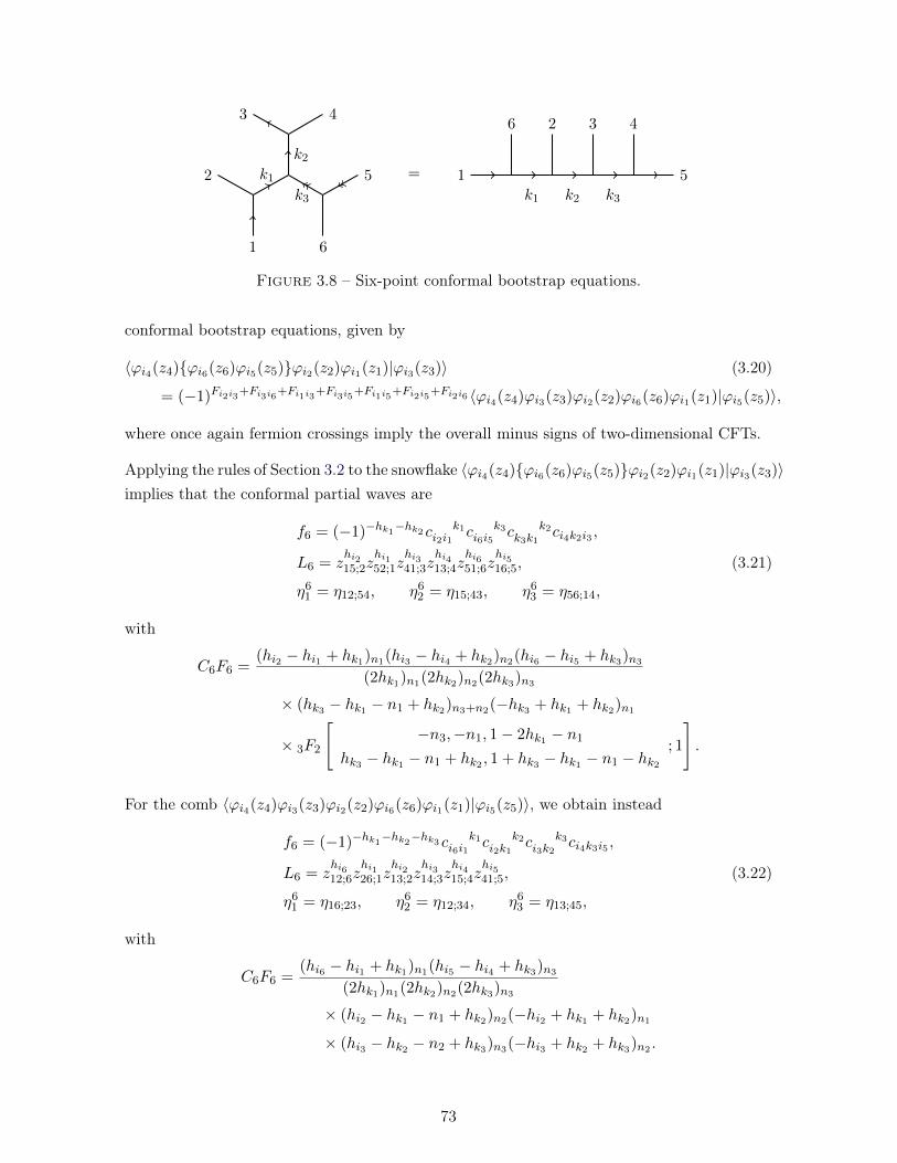
k1

1

2

k2

3 4

k3

5

6

= 1

6 2 3 4

5k1 k2 k3

Figure 3.8 – Six-point conformal bootstrap equations.

conformal bootstrap equations, given by

〈ϕi4(z4){ϕi6(z6)ϕi5(z5)}ϕi2(z2)ϕi1(z1)|ϕi3(z3)〉 (3.20)

= (−1)Fi2i3+Fi3i6+Fi1i3+Fi3i5+Fi1i5+Fi2i5+Fi2i6 〈ϕi4(z4)ϕi3(z3)ϕi2(z2)ϕi6(z6)ϕi1(z1)|ϕi5(z5)〉,

where once again fermion crossings imply the overall minus signs of two-dimensional CFTs.

Applying the rules of Section 3.2 to the snowflake 〈ϕi4(z4){ϕi6(z6)ϕi5(z5)}ϕi2(z2)ϕi1(z1)|ϕi3(z3)〉implies that the conformal partial waves are

f6 = (−1)−hk1−hk2 c k1

i2i1c k3i6i5

c k2k3k1

ci4k2i3 ,

L6 = zhi215;2z

hi152;1z

hi341;3z

hi413;4z

hi651;6z

hi516;5, (3.21)

η61 = η12;54, η6

2 = η15;43, η63 = η56;14,

with

C6F6 =(hi2 − hi1 + hk1)n1(hi3 − hi4 + hk2)n2(hi6 − hi5 + hk3)n3

(2hk1)n1(2hk2)n2(2hk3)n3

× (hk3 − hk1 − n1 + hk2)n3+n2(−hk3 + hk1 + hk2)n1

× 3F2

[−n3,−n1, 1− 2hk1 − n1

hk3 − hk1 − n1 + hk2 , 1 + hk3 − hk1 − n1 − hk2

; 1

].

For the comb 〈ϕi4(z4)ϕi3(z3)ϕi2(z2)ϕi6(z6)ϕi1(z1)|ϕi5(z5)〉, we obtain instead

f6 = (−1)−hk1−hk2

−hk3 c k1i6i1

c k2i2k1

c k3i3k2

ci4k3i5 ,

L6 = zhi612;6z

hi126;1z

hi213;2z

hi314;3z

hi415;4z

hi541;5, (3.22)

η61 = η16;23, η6

2 = η12;34, η63 = η13;45,

with

C6F6 =(hi6 − hi1 + hk1)n1(hi5 − hi4 + hk3)n3

(2hk1)n1(2hk2)n2(2hk3)n3

× (hi2 − hk1 − n1 + hk2)n2(−hi2 + hk1 + hk2)n1

× (hi3 − hk2 − n2 + hk3)n3(−hi3 + hk2 + hk3)n2 .

73

k1

1

2

k3

3 k4

4

5

k2

6

7

=

3

4 2 1 7 5

6k1 k2 k3 k4

Figure 3.9 – Seven-point conformal bootstrap equations.

Starting from the six-point conformal bootstrap equations (3.20) for all external quasi-primaryoperators, using the conformal partial wave decomposition (3.9) with the results (3.21) and(3.22), generates the full six-point conformal bootstrap.

3.3.4 Seven-Point Correlation Functions

Seven-point correlation functions can be decomposed in conformal partial waves following twotopologies : the comb and the extended snowflake topologies (81; 78). They are depicted inFigure 3.9 with a given choice of OPE limits. The equality shown in Figure 3.9 translates into

〈ϕi7(z7){ϕi3(z3)ϕi5(z5)ϕi4(z4)}ϕi2(z2)ϕi1(z1)|ϕi6(z6)〉 (3.23)

= (−1)Fi1i2+Fi1i3+Fi1i4+Fi2i3+Fi2i4+Fi3i4+Fi3i5+Fi5i7

× 〈ϕi5(z5)ϕi7(z7)ϕi1(z1)ϕi2(z2)ϕi4(z4)ϕi3(z3)|ϕi6(z6)〉,

and represents the sole set of seven-point conformal bootstrap equations, when consideringall external quasi-primary operators. In (3.23), the minus sign takes into account fermioncrossings that are possible in two-dimensional CFTs only.

Looking at the extended snowflake topology with the choice of OPE limits seen in Figure 3.9,i.e. the seven-point correlation functions 〈ϕi7(z7){ϕi3(z3)ϕi5(z5)ϕi4(z4)}ϕi2(z2)ϕi1(z1)|ϕi6(z6)〉,the conformal partial waves are

f7 = (−1)−hk1−hk2

−hk4 c k1i2i1

c k2k3k1

c k3i3k4

c k4i5i4

ci7k2i6 ,

L7 = zhi214;2z

hi142;1z

hi341;3z

hi543;5z

hi435;4z

hi716;7z

hi671;6, (3.24)

η71 = η12;47, η7

2 = η14;76, η73 = η43;17, η7

4 = η45;31,

74

with

C7F7 =(hi2 − hi1 + hk1)n1(hi6 − hi7 + hk2)n2(hi5 − hi4 + hk4)n4

(2hk1)n1(2hk2)n2(2hk3)n3(2hk4)n4

× (hi3 − hk4 − n4 + hk3)n3(−hi3 + hk4 + hk3)n4

× (hk3 − hk1 − n1 + hk2)n3+n2(−hk3 + hk1 + hk2)n1

× 3F2

[−n3,−n1, 1− 2hk1 − n1

hk3 − hk1 − n1 + hk2 , 1 + hk3 − hk1 − n1 − hk2

; 1

].

Focusing on 〈ϕi5(z5)ϕi7(z7)ϕi1(z1)ϕi2(z2)ϕi4(z4)ϕi3(z3)|ϕi6(z6)〉 instead, which corresponds tothe comb topology of Figure 3.9, we get

f7 = (−1)−hk1−hk2

−hk3−hk4 c k1

i4i3c k2i2k1

c k3i1k2

c k4i7k3

ci5k4i6 ,

L7 = zhi432;4z

hi324;3z

hi231;2z

hi137;1z

hi735;7z

hi536;5z

hi653;6, (3.25)

η71 = η34;21, η7

2 = η32;17, η73 = η31;75, η7

4 = η37;56,

with

C7F7 =(hi4 − hi3 + hk1)n1(hi6 − hi5 + hk4)n4

(2hk1)n1(2hk2)n2(2hk3)n3(2hk4)n4

× (hi2 − hk1 − n1 + hk2)n2(−hi2 + hk1 + hk2)n1

× (hi1 − hk2 − n2 + hk3)n3(−hi1 + hk2 + hk3)n2

× (hi7 − hk3 − n3 + hk4)n4(−hi7 + hk3 + hk4)n3 ,

As usual, comparing the conformal partial wave decomposition (3.9) of the seven-point correla-tion functions appearing in (3.23) that are given by (3.24) and (3.25) generate the seven-pointconformal bootstrap.

3.3.5 Eight-Point Correlation Functions

As a final example, we consider eight-point correlation functions for which there are fourdifferent topologies. The three independent eight-point conformal bootstrap equations areshown in Figure 3.10. They translate to

〈ϕi8(z8){{ϕi6(z6)ϕi5(z5)}ϕi4(z4)ϕi3(z3)}ϕi2(z2)ϕi1(z1)|ϕi7(z7)〉

= (−1)Fi1i2+Fi1i3+Fi1i4+Fi1i5+Fi6i8 〈ϕi6(z6)ϕi8(z8)ϕi1(z1){ϕi5(z5)ϕi4(z4)}ϕi3(z3)ϕi2(z2)|ϕi7(z7)〉

= (−1)Fi1i7+Fi2i7+Fi3i7+Fi4i7+Fi5i7+Fi6i7+Fi1i8+Fi2i8+Fi3i8+Fi4i8+Fi5i8+Fi6i8+Fi7i8

× 〈ϕi7(z7)ϕi6(z6){ϕi5(z5)ϕi4(z4)}ϕi3(z3)ϕi2(z2)ϕi1(z1)|ϕi8(z8)〉 (3.26)

= (−1)Fi1i7+Fi2i7+Fi3i7+Fi4i7+Fi5i7+Fi6i7+Fi1i8+Fi2i8+Fi3i8+Fi4i8+Fi5i8+Fi6i8+Fi7i8

× 〈ϕi7(z7)ϕi6(z6)ϕi5(z5)ϕi4(z4)ϕi3(z3)ϕi2(z2)ϕi1(z1)|ϕi8(z8)〉,

75

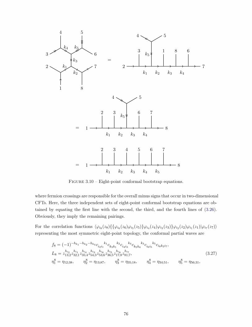
k1

1

2

k3

k4

3

4

k5

5

6

k2

7

8

=

2

3k5

4 5

1 8 6

7k1 k2 k3 k4

= 1

2 3k5

4 5

6 7

8k1 k2 k3 k4

= 1

2 3 4 5 6 7

8k1 k2 k3 k4 k5

Figure 3.10 – Eight-point conformal bootstrap equations.

where fermion crossings are responsible for the overall minus signs that occur in two-dimensionalCFTs. Here, the three independent sets of eight-point conformal bootstrap equations are ob-tained by equating the first line with the second, the third, and the fourth lines of (3.26).Obviously, they imply the remaining pairings.

For the correlation functions 〈ϕi8(z8){{ϕi6(z6)ϕi5(z5)}ϕi4(z4)ϕi3(z3)}ϕi2(z2)ϕi1(z1)|ϕi7(z7)〉representing the most symmetric eight-point topology, the conformal partial waves are

f8 = (−1)−hk1−hk2

−hk4 c k1i2i1

c k2k3k1

c k4i4i3

c k3k5k4

c k5i6i5

ci8k2i7 ,

L8 = zhi213;2z

hi132;1z

hi435;4z

hi354;3z

hi653;6z

hi536;5z

hi817;8z

hi781;7, (3.27)

η81 = η12;38, η8

2 = η13;87, η83 = η35;18, η8

4 = η34;51, η85 = η56;31,

76

with

C8F8 =(hi2 − hi1 + hk1)n1(hi7 − hi8 + hk2)n2(hi4 − hi3 + hk4)n4(hi6 − hi5 + hk5)n5

(2hk1)n1(2hk2)n2(2hk3)n3(2hk4)n4(2hk5)n5

× (hk3 − hk1 − n1 + hk2)n3+n2(−hk3 + hk1 + hk2)n1

× 3F2

[−n3,−n1, 1− 2hk1 − n1

hk3 − hk1 − n1 + hk2 , 1 + hk3 − hk1 − n1 − hk2

; 1

]× (hk5 − hk4 − n4 + hk3)n5+n3(−hk5 + hk4 + hk3)n4

× 3F2

[−n5,−n4, 1− 2hk4 − n4

hk5 − hk4 − n4 + hk3 , 1 + hk5 − hk4 − n4 − hk3

; 1

].

In the case of 〈ϕi6(z6)ϕi8(z8)ϕi1(z1){ϕi5(z5)ϕi4(z4)}ϕi3(z3)ϕi2(z2)|ϕi7(z7)〉, we have instead

f8 = (−1)−hk1−hk2

−hk3−hk4 c k1

i3i2c k2k5k1

c k3i1k2

c k5i5i4

c k4i8k3

ci6k4i7 ,

L8 = zhi324;3z

hi243;2z

hi542;5z

hi425;4z

hi128;1z

hi826;8z

hi627;6z

hi762;7, (3.28)

η81 = η23;41, η8

2 = η24;18, η83 = η21;86, η8

4 = η28;67, η85 = η45;21,

with

C8F8 =(hi3 − hi2 + hk1)n1(hi7 − hi6 + hk4)n4(hi5 − hi4 + hk5)n5

(2hk1)n1(2hk2)n2(2hk3)n3(2hk4)n4(2hk5)n5

× (hi1 − hk2 − n2 + hk3)n3(−hi1 + hk2 + hk3)n2

× (hi8 − hk3 − n3 + hk4)n4(−hi8 + hk3 + hk4)n3

× (hk5 − hk1 − n1 + hk2)n5+n2(−hk5 + hk1 + hk2)n1

× 3F2

[−n5,−n1, 1− 2hk1 − n1

hk5 − hk1 − n1 + hk2 , 1 + hk5 − hk1 − n1 − hk2

; 1

].

For 〈ϕi7(z7)ϕi6(z6){ϕi5(z5)ϕi4(z4)}ϕi3(z3)ϕi2(z2)ϕi1(z1)|ϕi8(z8)〉, the conformal partial wavesare

f8 = (−1)−hk1−hk2

−hk3−hk4 c k1

i2i1c k2i3k1

c k3k5k2

c k5i5i4

c k4i6k3

ci7k4i8 ,

L8 = zhi213;2z

hi132;1z

hi314;3z

hi541;5z

hi415;4z

hi617;6z

hi718;7z

hi871;8, (3.29)

η81 = η12;34, η8

2 = η13;46, η83 = η14;67, η8

4 = η16;78, η85 = η45;16,

with

C8F8 =(hi2 − hi1 + hk1)n1(hi8 − hi7 + hk4)n4(hi5 − hi4 + hk5)n5

(2hk1)n1(2hk2)n2(2hk3)n3(2hk4)n4(2hk5)n5

× (hi3 − hk1 − n1 + hk2)n2(−hi3 + hk1 + hk2)n1

× (hi6 − hk3 − n3 + hk4)n4(−hi6 + hk3 + hk4)n3

× (hk5 − hk2 − n2 + hk3)n5+n3(−hk5 + hk2 + hk3)n2

× 3F2

[−n5,−n2, 1− 2hk2 − n2

hk5 − hk2 − n2 + hk3 , 1 + hk5 − hk2 − n2 − hk3

; 1

].

77

Finally, for 〈ϕi7(z7)ϕi6(z6)ϕi5(z5)ϕi4(z4)ϕi3(z3)ϕi2(z2)ϕi1(z1)|ϕi8(z8)〉, we obtain the confor-mal partial waves for the comb topology as

f8 = (−1)−hk1−hk2

−hk3−hk4

−hk5 c k1i2i1

c k2i3k1

c k3i4k2

c k4i5k3

c k5i6k4

ci7k5i8 ,

L8 = zhi213;2z

hi132;1z

hi314;3z

hi415;4z

hi516;5z

hi617;6z

hi718;7z

hi871;8, (3.30)

η81 = η12;34, η8

2 = η13;45, η83 = η14;56, η8

4 = η15;67, η85 = η16;78,

with

C8F8 =(hi2 − hi1 + hk1)n1(hi8 − hi7 + hk5)n5

(2hk1)n1(2hk2)n2(2hk3)n3(2hk4)n4(2hk5)n5

× (hi3 − hk1 − n1 + hk2)n2(−hi3 + hk1 + hk2)n1

× (hi4 − hk2 − n2 + hk3)n3(−hi4 + hk2 + hk3)n2

× (hi5 − hk3 − n3 + hk4)n4(−hi5 + hk3 + hk4)n3

× (hi6 − hk4 − n4 + hk5)n5(−hi6 + hk4 + hk5)n4 .

Therefore, equating the conformal partial wave decompositions (3.9) of eight-point correlationfunctions as in (3.26), using the conformal partial waves (3.27), (3.28), (3.29), and (3.30), givesrise to the complete eight-point conformal bootstrap.

In this chapter, we proposed and proved a full set of Feynman-like rules, which can be used todirectly write down any global conformal partial wave in one- and two-dimensional CFTs. Withthe help of the known position space OPE, we proved the Feynman-like rules by construction.With our results, one can directly write down the kinematical part appearing in conformalcorrelation functions, which are completely fixed by conformal invariance. Hence, with theknowledge of dynamical part, i.e. CFT data constituting of the spectrum of quasi-primaryoperators with their dimensions h and h as well as the OPE coefficients, it is straightforwardto deduce any global M -point correlation function.

The Feynman-like rules that we introduced in this chapter give us a hint of the Feynman-likerules for scalar M -point conformal partial waves with scalar exchanges in higher-dimensionalCFTs. Indeed, the gluing procedure introduced in this chapter works in any dimensions. Thus,it is natural to expect that after decomposing higher-dimensional M -point conformal partialwaves into a set of vertices, one can associate the corresponding Feynman-like rules with eachvertex. The generalization of the rules to higher-dimensional conformal field theories, includingthe extra conformal cross-ratios, for scalar conformal blocks with any choice of OPE limitswill be presented in a forthcoming publication (118).

78

Chapitre 4

Symmetry Properties of theConformal Partial Waves

In Chapter 2, we verified the limit of unit operator and the OPE limit for the scalar M -point conformal partial waves with scalar exchanges in the comb configuration (2.9), (2.10),(2.11), and (2.14), the scalar six-point conformal partial waves with scalar exchanges in thesnowflake configuration (2.27), (2.28), (2.29), and (2.30) as well as scalar seven-point conformalpartial waves with scalar exchanges in the extended snowflake configuration (2.39), (2.40),(2.42), and (2.43). Besides verifying these asymptotical behaviours, the conformal partial wavesalso enjoy certain symmetries, which provide other consistency conditions. We denote thesymmetry group for a given M -point conformal partial wave by HM |topology. Each elementof the symmetry group corresponds to a symmetry transformation of the M -point conformalpartial wave, i.e. acting with a symmetry element transforms the diagram for the given M -point conformal partial wave back to itself. As a consequence, the expression for the conformalpartial waves must verify several identities related to the symmetry group HM |channel wherethe legs, conformal cross-ratios and the blocks are transformed according to the symmetries.

In this chapter, we study such symmetry group of the conformal partial waves and verify thesymmetry properties of the conformal partial waves which have been computed in Chapter 2.This chapter is based on work in (79; 80; 81).

4.1 M-point conformal partial waves with the comb topology

From Figure 2.1, it is easy to check that the scalarM -point conformal partial waves with scalarexchanges in the comb configuration are invariant under the transformations, including (1) theinterchange between Oi2(η2) and Oi3(η3), (2) the interchange between OiM (ηM ) and Oi1(η1),(3) the refection, which can be generated by switching the external operators Oia(ηa) andOiM+3−a(ηM+3−a), with 2 ≤ a ≤ bM+3

2 c and the understanding that OiM+1(ηM+1) ≡ Oi1(η1),

79

Oi2 Oi1

Oi3

. . .

OiM

Oi2 Oi1

Oi3

. . .

OiM

Figure 4.1 – Symmetries of the scalar M -point conformal partial waves in the comb configu-ration. The figure shows the two generators, with reflections on the left and dendrite permu-tations on the right.

as well as switching the internal operators Oka ↔ OkM−2−a , with 1 ≤ a ≤ bM−22 c. For obvious

reason, we dub the first two transformations the dendrite permutations. The correspondingsymmetry group is HM |comb = (Z2)2 o Z2, the semi-direct product of the direct product oftwo cyclic groups Z2 of order two, which corresponds to the two dendrite permutations, andthe cyclic group Z2 of order two, which corresponds to the reflection. The semi-direct productreflects the fact that the two dendrite permutations do not commute with the reflection.Moreover, we note that although (Z2)2 o Z2 contains eight group elements, all symmetrytransformations for the scalar M -point conformal partial waves with scalar exchanges in thecomb configuration can be generated by the dendrite permutation Oi2(η2)↔ Oi3(η3), and thereflection, illustrated in Figure 4.1. As a consequence, only the dendrite permutationOi2(η2)↔Oi3(η3) and the reflection need to be verified for the scalar M -point conformal partial waveswith scalar exchanges in the comb configuration. To verify the symmetry properties, one needto first implement the symmetry transformation on the legs LM |comb, the conformal cross-ratios ua and vab, as well as the blocks GM |comb and then prove that the original conformalpartial waves (2.9), (2.10), (2.11), and (2.14) are equivalent to the conformal partial wavesbuilt from the new legs, conformal cross-ratios, and blocks. Again, the proofs rely on therepetitive use of (2.3) and (2.4). In Appendix F, we verify the symmetry properties of thescalar six-point conformal partial waves with scalar exchanges in the snowflake configuration(2.27), (2.28), (2.29), and (2.30). The proofs there can be straightforwardly generalized toverify the symmetry properties for the M -point comb conformal partial waves discussed here.

4.2 Six-point conformal partial waves with the snowflaketopology

The diagram for the scalar six-point conformal partial waves with the scalar exchanges in thesnowflake configuration Figure 2.3 is more symmetric than the diagram for six-point combconformal partial waves. In other words, the order of the symmetry group for the six-pointsnowflake conformal partial waves is larger than the order of the group (Z2)2 o Z2, which isthe symmetry group for the six-point comb partial waves. Indeed, the snowflake diagram isinvariant under transformations including two rotations (rotations by 2π/3 and 4π/3), three

80

Ok1

Oi2

Oi3Ok2

Oi5Oi4

Ok3

Oi6

Oi1

Ok1

Oi2

Oi3Ok2

Oi5Oi4

Ok3

Oi6

Oi1

Ok1

Oi2

Oi3Ok2

Oi5Oi4

Ok3

Oi6

Oi1

Figure 4.2 – Symmetries of the scalar six-point conformal blocks in the snowflake channel.The figure shows rotations by 2π/3 (left), reflections (middle), and dendrite permutations(right).

reflections (reflections along three different axis), and three dendrite permutations. We notethat the rotations and reflections generate the dihedral group of order six, D3, which is thesymmetry group of both equilateral triangle and three-point conformal correlation functions.The three dendrite permutations generate the symmetry group (Z2)3 of order eight, which isthe direct product of three cyclic groups Z2. As a consequence, the full symmetry group forscalar six-point conformal partial waves with the scalar exchanges in the snowflake configura-tion is H6|snowflake = (Z2)3 oD3. Again, the use of semi-direct product reflects the fact thatthe rotations and reflections do not commute with the three dendrite permutations.

Although we dubbed it the snowflake topology, the full symmetry group is not the dihedralgroup of order twelve, D6, which is the symmetry group for hexagon. Since the order of thesymmetry group for snowflake conformal partial waves is |(Z2)3 o D3| = 48, the snowflakediagram has a larger symmetry group than the hexagon, contrary to expectations.

At the first glance, we have to verify 47 identities for the scalar six-point conformal partialwaves with scalar exchanges in the snowflake configuration (2.27), (2.28), (2.29), and (2.30)since the order of the symmetry group (Z2)3 o D3 is 48. However, it is easy to check thatthe full symmetry group (Z2)3 o D3 can be generated by three elements including rotationsby 2π/3, reflections, and dendrite permutations, shown in Figure 4.2. Therefor, only threeidentities are necessary to be checked, to which we now turn.

4.2.1 Rotations

After rotating the six-point snowflake diagram by 2π/3, the quasi-primary operators transformas Oia(ηa) → Oia+2(ηa+2) and Oka → Oka+1 with the understanding that Oi7(η7) ≡ Oi1(η1),Oi8(η8) ≡ Oi2(η2) as well as Ok4 ≡ Ok1 . Under this transformation, the legs (2.27) andconformal cross-ratios (2.28) transform as

L6

∏1≤a≤3

(u6a)

∆ka2 → L6

∏1≤a≤3

(u6a)

∆ka2 ,

81

and

u61 → u6

2, u62 → u6

3, u63 → u6

1,

v611 → v6

12, v612 → v6

23, v613 → v6

22,

v622 → v6

33, v623 → v6

11, v633 → v6

13,

respectively. The fact that the scalar six-point conformal partial waves with the scalar ex-changes in the snowflake configuration is invariant under this transformation translate intothe following identity,

G(d,h2,h3,h4,h5;p2,p3,p4,p5,p6)6|snowflake (u6

1, u62, u

63; v6

11, v612, v

613, v

622, v

623, v

633) (4.1)

= G(d,−p3,h4,h5,h3;p3−h2,p2+h2,p5,p6,p4)6|snowflake (u6

2, u63, u

61; v6

12, v623, v

622, v

633, v

611, v

613).

Using the known C-function for the scalar six-point conformal partial waves with the scalarexchanges in the snowflake configuration (2.29), it is easy to see that C6|snowflake is invariantunder this rotation generator, resulting in a non-trivial identity for F6,

F(d,h2,h3,h4,h5;p2,p3,p4,p5,p6)6|snowflake (m1,m2,m3) = F

(d,−p3,h4,h5,h3;p3−h2,p2+h2,p5,p6,p4)6|snowflake (m2,m3,m1).

To simplify the notation, we denote the above identity by F6 = F6R. To prove F6 = F6R, wefirst rewrite (2.30) as

F6 =(−p3 + h2 + d/2−m2)m2

(p3)−m1(−h2 +m1 +m2)−m3

∑t1,t2≥0

(−m1)t2(−m2)t1(−m3)t2(p3 − h2 − d/2 + 1)t1

× (p3)t1(p3 − d/2)t1(−p2 + d/2−m1)t2(1 + h2 −m1 +m3 −m2)m2−t1(1 + h2 −m1 −m2)m2−t1+t2(p3 −m1)t1+t2t1!t2!

,

and then use the identity

(1 + h2 −m1 +m3 −m2)m2−t1(1 + h2 −m1 −m2)m2−t1+t2

=(1 + h2 −m1 +m3 −m2)m2−t1

(1 + h2 −m1 −m2 + t2)m2−t(1 + h2 −m1 −m2)t2

=∑t3≥0

(−m3 + t2)t3(−m2 + t1)t3(1 + h2 −m1 −m2 + t2)t3(1 + h2 −m1 −m2)t2t3!

,

to express F6 as

F6 =(−p3 + h2 + d/2−m2)m2

(p3)−m1(−h2 +m1 +m2)−m3

∑t1,t2,t3≥0

(−m1)t2(−m2)t1+t3(−m3)t2+t3

(p3 − h2 − d/2 + 1)t1

× (p3)t1(p3 − d/2)t1(−p2 + d/2−m1)t2(1 + h2 −m1 −m2)t2+t3(p3 −m1)t1+t2t1!t2!t3!

.

We now modify the sum over t1 with the help of (2.4), to get

F6 =∑

t1,t2,t3≥0

(−m1)t1+t2(−m2)t1+t3(−m3)t2+t3

(p3)−m1(p2 + h2)−m2(−h2 +m1 +m2)−m3t1!t2!t3!(4.2)

× (p3 − d/2)t1(−p2 + d/2−m1)t2(−p3 + h2 + d/2−m2)t3(p3 −m1)t1+t2(p2 + h2 −m2)t1+t3(1 + h2 −m1 −m2)t2+t3

.

82

We can use (2.4) again to obtain

F6 =∑

t2,t3≥0

(−m1)t2(−m2)t3(−m3)t2+t3

(−p2 + d/2)−m1(p2 + h2)−m2(−h2 +m1 +m2)−m3t2!t3!

× (−p3 + h2 + d/2−m2)t3(p2 + h2 −m2)t3(1 + h2 −m1 −m2)t2+t3

3F2

[−m1 + t2, p3 − d/2, p2 + h2

p2 + 1− d/2, p2 + h2 −m2 + t3; 1

].

It is now possible to expand the 3F2-hypergeometric function as a summation over t1 andevaluate the sum over t2 with the help of (2.3), leading to

F6 =∑

t1,t3≥0

(−m1)t1(−m2)t3(−m3)t3(−p2 + d/2)−m1(p2 + h2)−m2(−h2 +m1 +m2)−m3t1!t3!

× (1 + h2 −m1 −m2 +m3)m1−t1(p3 − d/2)t1(p2 + h2)t1(−p3 + h2 + d/2−m2)t3(p2 + 1− d/2)t1(p2 + h2 −m2)t1+t3(1 + h2 −m1 −m2)m1−t1+t3

.

Expressing the sum over t3 as a 3F2-hypergeometric function and using (2.4) once more leadsto

F6 =∑t1≥0

(−h2 −m3 + t1)m3

(−p2 + d/2)−m1(p2 + h2)−m2

(−m1)t1(p3 − d/2)t1(p2 + h2)t1(p2 + 1− d/2)t1(p2 + h2 −m2)t1t1!

× 3F2

[−m2,−m3, p3 − d/2 + t1

−h2 −m3 + t1, p2 + h2 −m2 + t1; 1

]

=∑t1≥0

(−h2 −m3 + t1)m3

(−p2 + d/2)−m1(p2 + h2)−m2

(−m1)t1(p3 − d/2)t1(p2 + h2)t1(p2 + 1− d/2)t1(p2 + h2 −m2)t1t1!

× 3F2

[−m2,−m3, p3 − d/2 + t1

p2 + h2 −m2 + t1,−h2 −m3 + t1; 1

],

where in the last equality we simply changed the order of the two bottom parameters of the

3F2-hypergeometric function. With this change, we can finally re-use (2.4) to get

F6 =∑t1≥0

(p2 + h2 −m2 +m3 + t1)m2

(−p2 + d/2)−m1(p2 + h2)−m2

(−m1)t1(p3 − d/2)t1(p2 + h2)t1(p2 + 1− d/2)t1(p2 + h2 −m2)m2+t1t1!

× (−h2 −m3 + t1)m33F2

[−m2,−m3,−p3 − h2 + d/2−m3

1− p2 − h2 −m3 − t1,−h2 −m3 + t1; 1

],

which is nothing else than F6 = F6R, completing the proof.

We note that the invariance of the F -function for the scalar six-point conformal partial waveswith the scalar exchanges in the snowflake configuration under rotations can be translated

83

into identities for Kampé de Fériet functions,

F 1,3,22,1,0

[a1;−m2, b1 +m3, b2 +m1;−m1,−m3

b1, b2; d1;−

∣∣∣∣∣ 1, 1]

=(d1 − a1)m2(b1 − a1)m3

(d1)m2(b1)m3

F 1,3,22,1,0

[a1; b2 +m1, 1 + a1 − d1,−m3;−m1,−m2

1 + a1 − d1 −m2, b2; 1 + a1 − b1 −m3;−

∣∣∣∣∣ 1, 1],

F 2,1,11,1,1

[a1, a2;−m2;−m3

a2 −m1; d1; g1

∣∣∣∣∣ 1, 1]

=(a2)−m1(d1 − a1)m2

(a2 − a1)−m1(d1)m2

F 2,1,11,1,1

[a1, 1 + a1 − d1;−m1;−m3

1 + a1 − d1 −m2, 1 + a1 − a2; g1

∣∣∣∣∣ 1, 1],

with

F 1,3,22,1,0

[a1;−m2, 1 + a1 − g1, a2;−m1,−m3

1 + a1 − g1 −m3, a2 −m1; d1;−

∣∣∣∣∣ 1, 1]

=(g1)m3

(g1 − a1)m3

F 2,1,11,1,1

[a1, a2;−m2;−m3

a2 −m1; d1; g1

∣∣∣∣∣ 1, 1],

for m1, m2, and m3 non-negative integers and a1, a2, b1, b2, d1, and g1 arbitrary.

4.2.2 Reflections

For reflections, depicted in Figure 4.2, it is easy to check the quasi-primary operators transformas

Oi2(η2)↔ Oi4(η4), Oi3(η3)↔ Oi5(η5), Ok1 ↔ Ok2 ,

under this transformation. As a result, for this reflection generator, the legs (2.27) and confor-mal cross-ratios (2.28) transform as

L6

∏1≤a≤3

(u6a)

∆ka2 → (v6

11)h3(v612)h4(v6

23)h5L6

∏1≤a≤3

(u6a)

∆ka2 ,

and

u61 →

u62

v612

, u62 →

u61

v611

, u63 →

u63

v623

,

v611 →

1

v612

, v612 →

1

v611

, v613 →

v633

v612v

623

,

v622 →

v622

v611v

612

, v623 →

1

v623

, v633 →

v613

v611v

623

,

respectively. The identity for I6|snowflake then translates into the identity for G6|snowflake,

G(d,h2,h3,h4,h5;p2,p3,p4,p5,p6)6|snowflake (u6

1, u62, u

63; v6

11, v612, v

613, v

622, v

623, v

633) (4.3)

= (v611)h3(v6

12)h4(v623)h5

×G(d,h2,h4,h3,h5;p3−h2,p2+h2,p5,p4,p6)6|snowflake

(u6

2

v612

,u6

1

v611

,u6

3

v623

;1

v612

,1

v611

,v6

33

v612v

623

,v6

22

v611v

612

,1

v623

,v6

13

v611v

623

).

84

We note the F -function (2.30) for the scalar six-point conformal partial waves with scalarexchanges in the snowflake configuration is manifestly invariant under the reflection symmetryillustrated in Figure 4.2. Indeed, this reflection symmetry of F6|snowflake can be directly seenfrom the expression (4.2). As a result, the identity (4.3) then implies an identity for C6snowflake.The identity (4.3) will be verified in Appendix F through the repetitive use of (2.3) and (2.4).

4.2.3 Dendrite permutations

The last generator in Figure 4.2 is the dendrite permutation, which switches the Oi2(η2) andOi3(η3). Under this transformation, the legs (2.27) and conformal cross-ratios transform as

L6

∏1≤a≤3

(u6a)

∆ka2 → (v6

11)h2−h4(v622)h4L6

∏1≤a≤3

(u6a)

∆ka2 ,

and

u61 →

u61

v611

, u62 →

u62

v622

, u63 → u6

3v611,

v611 →

1

v611

, v612 →

v611v

612

v622

, v613 → v6

23,

v622 →

1

v622

, v623 → v6

13, v633 →

v611v

633

v622

,

respectively. Therefore, the invariance of the scalar six-point conformal partial waves withscalar exchanges in the snowflake configuration under this transformation implies that

G(d,h2,h3,h4,h5;p2,p3,p4,p5,p6)6|snowflake (u6

1, u62, u

63; v6

11, v612, v

613, v

622, v

623, v

633) (4.4)

= (v611)h2−h4(v6

22)h4

×G(d,h2,−p2−h3,h4,h5;p2,p3,p4,p5,p6)6|snowflake

(u6

1

v611

,u6

2

v622

, u63v

611;

1

v611

,v6

11v612

v622

, v623,

1

v622

, v613,

v611v

633

v622

).

Once again, F -function (2.30) is invariant under this generator for dendrite permutations,resulting in a second identity for C6. The identity (4.4) will again be verified in Appendix F.

Since the full symmetry group (Z2)3 o D3 of order 48 can be generated by the above threegenerators by composition, the identities (4.1), (4.3), and (4.4), corresponding to rotations,reflections, and dendrite permutations, respectively, verify the symmetry properties of thescalar six-point conformal partial waves with scalar exchanges in the snowflake configuration(2.27), (2.28), (2.29), and (2.30).

4.3 Seven-point conformal partial waves with the extendedsnowflake topology

The scalar seven-point conformal partial waves with scalar exchanges in the extended snow-flake configuration is invariant under the three generators shown in Figure 4.3. These three

85

Ok2

Oi3

Oi4Ok3

Oi6Oi5

Ok1

Oi2

Ok4

Oi7

Oi1Ok2

Oi3

Oi4Ok3

Oi6Oi5

Ok1

Oi2

Ok4

Oi7

Oi1Ok2

Oi3

Oi4Ok3

Oi6Oi5

Ok1

Oi2

Ok4

Oi7

Oi1

Figure 4.3 – Symmetries of the scalar seven-point conformal partial waves with scalar ex-changes in the extended snowflake configuration. The figure shows the three generators withreflection (left), dendrite permutation of the first kind (middle), and dendrite permutation ofthe second kind (right).

generators generate the symmetry group H7|extendedsnowflake

= Z2 ×((Z2)2 o Z2

), which can be seen

as follows. The first Z2 subgroup generates the dendrite permutation of the second kind,which switch the external quasi-primary operators Oi1(η1) and Oi7(η7). The second and thirdcyclic groups, denoted by (Z2)2 in the symmetry group H

7|extendedsnowflake, is a direct product of

the Z2 which corresponds to the dendrite permutation Oi3(η3) ↔ Oi4(η4), and the Z2 whichcorresponds to the dendrite permutation Oi5(η5) ↔ Oi6(η6). We call the two dendrite per-mutations generated by (Z2)2 the dendrite permutations of the first kind. Finally, the lastZ2 subgroup corresponds to simultaneous reflections the external quasi-primary operatorsOi3(η3) ↔ Oi5(η5) and Oi4(η4) ↔ Oi6(η6) as well as the internal quasi-primary operatorsOk2 ↔ Ok3 . Its effect is to switch the two external dendrites associated to the (Z2)2 subgroup.This observation leads the semi-direct nature of the product (Z2)2 oZ2. Combining with thefact that both the dendrite permutations of the first kind and the refections commute withthe dendrite permutation of the second kind, we conclude that the full symmetry group isH

7|extendedsnowflake= Z2 ×

((Z2)2 o Z2

).

The fact that the order of the symmetry group H7|extendedsnowflake

is |H7|extendedsnowflake

| = 16 leads to fifteen

consistency conditions for our expressions (2.39), (2.40), (2.42), and (2.43) for the scalar seven-point conformal partial waves with scalar exchanges in the extended snowflake configuration.Since the full symmetry group H

7|extendedsnowflake= Z2×

((Z2)2 o Z2

)can be obtained from the three

generators of Figure 4.3, we only need to verify the three identities associated with these threegenerators.

4.3.1 Dendrite permutation of the second kind

The dendrite permutation of the second kind generates the transformation Oi1(η1)↔ Oi7(η7),under which the legs (2.39) and conformal cross-ratios (2.40) transform as

L7

∏1≤a≤4

(u7a)

∆ka2 → (v7

14)−p4L7

∏1≤a≤4

(u7a)

∆ka2 ,

86

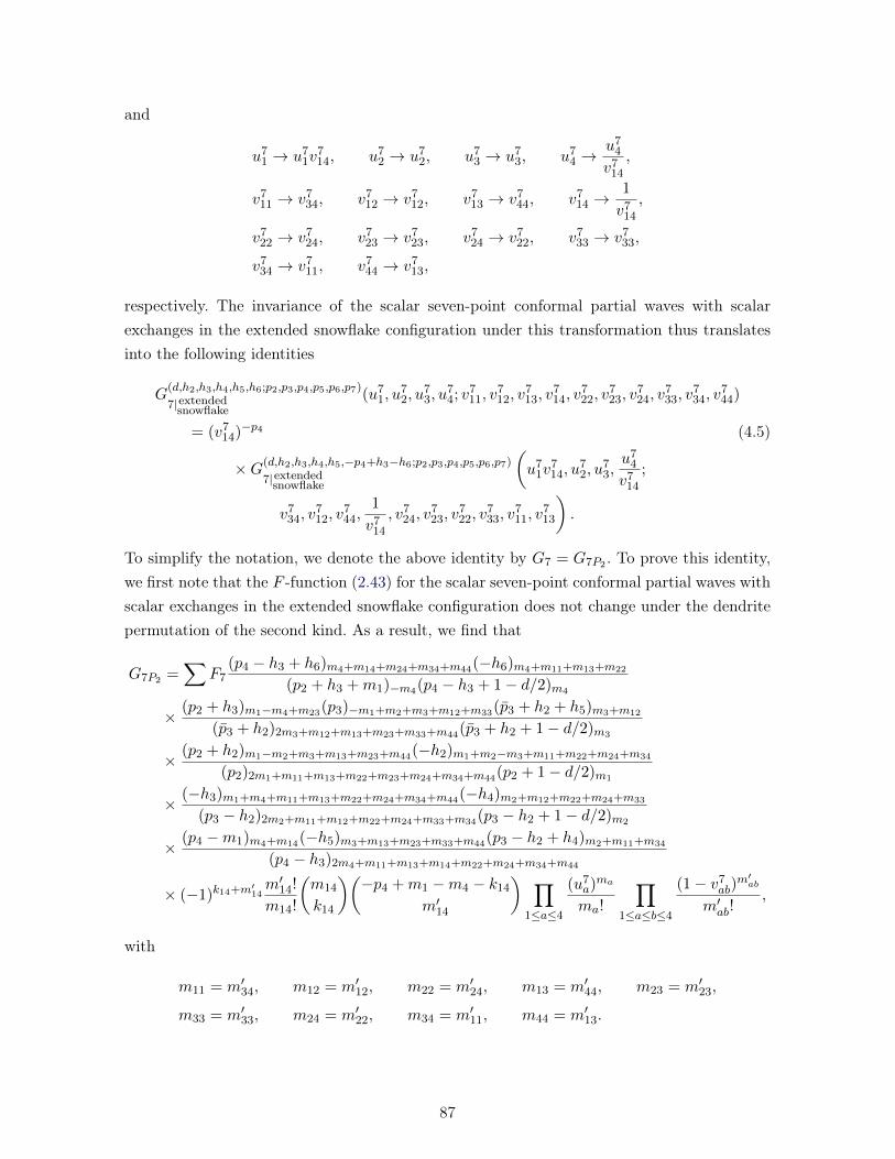
and

u71 → u7

1v714, u7

2 → u72, u7

3 → u73, u7

4 →u7

4

v714

,

v711 → v7

34, v712 → v7

12, v713 → v7

44, v714 →

1

v714

,

v722 → v7

24, v723 → v7

23, v724 → v7

22, v733 → v7

33,

v734 → v7

11, v744 → v7

13,

respectively. The invariance of the scalar seven-point conformal partial waves with scalarexchanges in the extended snowflake configuration under this transformation thus translatesinto the following identities

G(d,h2,h3,h4,h5,h6;p2,p3,p4,p5,p6,p7)

7|extendedsnowflake(u7

1, u72, u

73, u

74; v7

11, v712, v

713, v

714, v

722, v

723, v

724, v

733, v

734, v

744)

= (v714)−p4 (4.5)

×G(d,h2,h3,h4,h5,−p4+h3−h6;p2,p3,p4,p5,p6,p7)

7|extendedsnowflake

(u7

1v714, u

72, u

73,u7

4

v714

;

v734, v

712, v

744,

1

v714

, v724, v

723, v

722, v

733, v

711, v

713

).

To simplify the notation, we denote the above identity by G7 = G7P2 . To prove this identity,we first note that the F -function (2.43) for the scalar seven-point conformal partial waves withscalar exchanges in the extended snowflake configuration does not change under the dendritepermutation of the second kind. As a result, we find that

G7P2 =∑

F7(p4 − h3 + h6)m4+m14+m24+m34+m44(−h6)m4+m11+m13+m22

(p2 + h3 +m1)−m4(p4 − h3 + 1− d/2)m4

× (p2 + h3)m1−m4+m23(p3)−m1+m2+m3+m12+m33(p3 + h2 + h5)m3+m12

(p3 + h2)2m3+m12+m13+m23+m33+m44(p3 + h2 + 1− d/2)m3

× (p2 + h2)m1−m2+m3+m13+m23+m44(−h2)m1+m2−m3+m11+m22+m24+m34

(p2)2m1+m11+m13+m22+m23+m24+m34+m44(p2 + 1− d/2)m1

× (−h3)m1+m4+m11+m13+m22+m24+m34+m44(−h4)m2+m12+m22+m24+m33

(p3 − h2)2m2+m11+m12+m22+m24+m33+m34(p3 − h2 + 1− d/2)m2

× (p4 −m1)m4+m14(−h5)m3+m13+m23+m33+m44(p3 − h2 + h4)m2+m11+m34

(p4 − h3)2m4+m11+m13+m14+m22+m24+m34+m44

× (−1)k14+m′14m′14!

m14!

(m14

k14

)(−p4 +m1 −m4 − k14

m′14

) ∏1≤a≤4

(u7a)ma

ma!

∏1≤a≤b≤4

(1− v7ab)

m′ab

m′ab!,

with

m11 = m′34, m12 = m′12, m22 = m′24, m13 = m′44, m23 = m′23,

m33 = m′33, m24 = m′22, m34 = m′11, m44 = m′13.

87

Computing the sum over k14 leads to

G7P2 =∑ (p4 − h3 + h6)m4+m14+m24+m34+m44(−h6)m4+m11+m13+m22

(p2 + h3 +m1)−m4(p4 − h3 + 1− d/2)m4

× (p2 + h3)m1−m4+m23(p3)−m1+m2+m3+m12+m33(p3 + h2 + h5)m3+m12

(p3 + h2)2m3+m12+m13+m23+m33+m44(p3 + h2 + 1− d/2)m3

× (p2 + h2)m1−m2+m3+m13+m23+m44(−h2)m1+m2−m3+m11+m22+m24+m34

(p2)2m1+m11+m13+m22+m23+m24+m34+m44(p2 + 1− d/2)m1

× (−h3)m1+m4+m11+m13+m22+m24+m34+m44(−h4)m2+m12+m22+m24+m33

(p3 − h2)2m2+m11+m12+m22+m24+m33+m34(p3 − h2 + 1− d/2)m2

×(p4 −m1)m4+m′14

(−h5)m3+m13+m23+m33+m44(p3 − h2 + h4)m2+m11+m34

(p4 − h3)2m4+m11+m13+m14+m22+m24+m34+m44

× (−m′14)m14

m14!F7

∏1≤a≤4

(u7a)ma

ma!

∏1≤a≤b≤4

(1− v7ab)

m′ab

m′ab!.

We then evaluate the sum over m14, giving

G7P2 =∑ (p4 − h3 + h6)m4+m24+m34+m44(−h6)m4+m11+m13+m′14+m22

(p2 + h3 +m1)−m4(p4 − h3 + 1− d/2)m4

× (p2 + h3)m1−m4+m23(p3)−m1+m2+m3+m12+m33(p3 + h2 + h5)m3+m12

(p3 + h2)2m3+m12+m13+m23+m33+m44(p3 + h2 + 1− d/2)m3

× (p2 + h2)m1−m2+m3+m13+m23+m44(−h2)m1+m2−m3+m11+m22+m24+m34

(p2)2m1+m11+m13+m22+m23+m24+m34+m44(p2 + 1− d/2)m1

× (−h3)m1+m4+m11+m13+m22+m24+m34+m44(−h4)m2+m12+m22+m24+m33

(p3 − h2)2m2+m11+m12+m22+m24+m33+m34(p3 − h2 + 1− d/2)m2

×(p4 −m1)m4+m′14

(−h5)m3+m13+m23+m33+m44(p3 − h2 + h4)m2+m11+m34

(p4 − h3)2m4+m11+m13+m′14+m22+m24+m34+m44

× F7

∏1≤a≤4

(u7a)ma

ma!

∏1≤a≤b≤4

(1− v7ab)

m′ab

m′ab!

= G7,

which completes the proof of the identity (4.5).

4.3.2 Dendrite permutation of the first kind

The transformation of dendrite permutations of the first kind, depicted in Figure 4.3, switchesthe external quasi-primary operators Oi3(η3) and Oi4(η4). As a consequence, the legs (2.39)and conformal cross-ratios (2.40) change under this transformation as

L7

∏1≤a≤4

(u7a)

∆ka2 → (v7

12)−p3−h5(v733)h5L7

∏1≤a≤4

(u7a)

∆ka2 ,

88

and

u71 → u7

1v712, u7

2 →u7

2

v712

, u73 →

u73

v733

, u74 → u7

4,

v711 → v7

22, v712 →

1

v712

, v713 →

v712v

713

v733

, v714 → v7

14,

v722 → v7

11, v723 →

v712v

723

v733

, v724 → v7

34, v733 →

1

v733

,

v734 → v7

24, v744 →

v712v

744

v733

,

respectively. Hence, the corresponding identity for G7|extendedsnowflake

is given by

G(d,h2,h3,h4,h5,h6;p2,p3,p4,p5,p6,p7)

7|extendedsnowflake(u7

1, u72, u

73, u

74; v7

11, v712, v

713, v

714, v

722, v

723, v

724, v

733, v

734, v

744)

= (v712)−p3−h5(v7

33)h5

×G(d,h2,h3,−p3+h2−h4,h5,h6;p2,p3,p4,p5,p6,p7)

7|extendedsnowflake

(u7

1v712,

u72

v712

,u7

3

v733

, u74; (4.6)

v722,

1

v712

,v7

12v713

v733

, v714, v

711,

v712v

723

v733

, v734,

1

v733

, v724,

v712v

744

v733

).

Again, the F -function (2.43) for the scalar seven-point conformal partial waves with scalarexchanges in the extended snowflake configuration is invariant under dendrite permutationsof the first kind. The proof for the identity (4.6) is analogous to the proof for (4.5) but withlonger and more tedious computations. As such, we do not present it here.

4.3.3 Reflections

The reflection generator in Figure 4.3 changes the quasi-primary operators as

Oi3(η3)↔ Oi5(η5), Oi4(η4)↔ Oi6(η6), Ok2 ↔ Ok3 ,

leading to the transformations of the legs (2.39) and conformal cross-ratios (2.40), which aregiven by

L7

∏1≤a≤4

(u7a)

∆ka2 → (v7

11)h3−h6(v712)h4(v7

23)h5(v734)h6L7

∏1≤a≤4

(u7a)

∆ka2 ,

and

u71 →

u71

v711

, u72 →

u73

v723

, u73 →

u72

v712

, u74 →

u74

v734

,

v711 →

1

v711

, v712 →

1

v723

, v713 →

v722

v711v

712

, v714 →

v711v

714

v734

,

v722 →

v713

v711v

723

, v723 →

1

v712

, v724 →

v744

v723v

734

, v733 →

v733

v712v

723

,

v734 →

1

v734

, v744 →

v724

v712v

734

,

89

respectively. Then, the fact that the scalar seven-point conformal partial waves with scalarexchanges in the extended snowflake configuration is invariant under this reflection impliesthe following identity,

G(d,h2,h3,h4,h5,h6;p2,p3,p4,p5,p6,p7)

7|extendedsnowflake(u7

1, u72, u

73, u

74; v7

11, v712, v

713, v

714, v

722, v

723, v

724, v

733, v

734, v

744)

= (v711)h3−h6(v7

12)h4(v723)h5(v7

34)h6 (4.7)

×G(d,−p2−h2,h3,h5,h4,h6;p2,p3,p4,p6,p5,p7)

7|extendedsnowflake

(u7

1

v711

,u7

3

v723

,u7

2

v712

,u7

4

v734

;

1

v711

,1

v723

,v7

22

v711v

712

,v7

11v714

v734

,v7

13

v711v

723

,1

v712

,v7

44

v723v

734

,v7

33

v712v

723

,1

v734

,v7

24

v712v

734

).

Once again, the F -function (2.43) for the scalar seven-point conformal partial waves withscalar exchanges in the extended snowflake configuration does not change under the reflectiongenerator. The proof for the identity (4.7) is analogous to the proof for (4.5). As such, we donot present it here.

In this chapter, we verified the symmetry properties of the conformal partial waves computedin Chapter 2. As we have seen, the symmetry group HM |topology of the conformal partial wavesIM |topology imposes a set of consistency conditions. The fact that our results for the scalar M -point conformal partial waves with scalar exchanges in the comb configuration (2.9), (2.10),(2.11), and (2.14), the scalar six-point conformal partial waves with scalar exchanges in thesnowflake configuration (2.27), (2.28), (2.29), and (2.30) as well as scalar seven-point confor-mal partial waves with scalar exchanges in the extended snowflake configuration (2.39), (2.40),(2.42), and (2.43) pass these consistency conditions lends further credence to the embeddingspace OPE formalism developed in Chapter 1. Moreover, we also note that the symmetry ofthe conformal partial waves IM |topology is a subgroup of the symmetry group of the correspon-ding M -point conformal correlation functions. Indeed, the symmetry group of the M -pointconformal correlation functions is SM , i.e. the permutation group of M elements. 1 The studyof cosets SM/HM |channel, whose elements generate symmetry transformations for M -pointconformal correlation functions but switch the conformal partial waves into different channels,leads to interesting consequences, to which we now turn.

1. Although permutating fermionic quasi-primary operators may introduce an extra minus sign, our dis-cussion here as well as in the next chapter does not change.

90

Chapitre 5

Conformal Bootstrap Equations

In this chapter we discuss the conformal bootstrap equations for M -point conformal correla-tion functions. The discussion here is based on the work of my collaborators and me (80). Thecrucial idea behind the conformal bootstrap program is the crossing symmetry, which is thesymmetry of the conformal correlation functions. Using the conformal partial wave expansion,we can classify the full symmetry group SM of the M -point conformal correlation functionsinto two parts. One part consists of elements, which generate the symmetry transformationsfor both conformal correlation functions and conformal partial waves IM |topology, while anotherpart consists of elements, which generate the symmetry transformation for conformal corre-lation functions but switch the conformal partial waves IM |topology into different channels.Clearly, the former is nothing but the symmetry group HM |topology of the conformal partialwaves IM |topology discussed in Chapter 4, and the latter is the coset SM/HM |topology. We notethat the invariance of the conformal partial waves IM |topology under the transformations ge-nerated by HM |topology makes the invariance of the M -point conformal correlation functionsholds automatically. As a result, only the study of the cosets SM/HM |topology leads to non-trivial consequences. Indeed, the study of the cosets SM/HM |topology is directly related to theconformal bootstrap program.

To illuminate the above discussion, we take the four-point conformal correlation function〈oi1(x1)oi2(x2)oi3(x3)oi4(x4)〉 as an example. Using the OPE, the conformal partial wave ex-pansion for the four-point conformal correlation functions is given by

〈{oi1(x1)oi2(x2)}{oi3(x3)oi4(x4)}〉 =∑k

Ni1i2k∑a=1

Ni3i4k∑b=1

Ii1i2i3i4k(x1, x2, x3, x4),

where we absorbed the OPE coefficients into the conformal partial waves Ii1i2i3i4 k(x1, x2, x3, x4).Since we have proved in Chapter 4 that the conformal partial waves Ii1i2i3i4 k(x1, x2, x3, x4) donot change under the symmetry group H4|comb = (Z2)2oZ2, it is apparent that the four-pointcorrelation functions also do not change under H4|comb = (Z2)2 o Z2. However, under theswitch of oi1(x1) and oi4(x4), which can be generated by elements in the coset S4/H4|comb, the

91

conformal partial waves Ii1i2i3i4 k(x1, x2, x3, x4) change to the conformal partial waves in thet-channel Ii4i2i3i1 k

′(x4, x2, x3, x1) 6= Ii1i2i3i4

k(x1, x2, x3, x4). Then, the fact that the four-pointconformal correlation functions are invariant under this transformation implies the followingnon-trivial identity

〈{oi1(x1)oi2(x2)}{oi3(x3)oi4(x4)}〉 = 〈{oi4(x4)oi2(x2)}{oi3(x3)oi1(x1)}〉,

or

∑k

Ni1i2k∑a=1

Ni3i4k∑b=1

Ii1i2i3i4k(x1, x2, x3, x4) =

∑k′

Ni4i2k′∑a=1

Ni3i1k′∑b=1

Ii4i2i3i1k′(x4, x2, x3, x1),

which is nothing but the conformal bootstrap equation identifying the s- and u-channel confor-mal partial wave expansions. It is easy to check that other two elements in the coset S4/H4|comb

of order three generate the s- and t-channel conformal partial waves, respectively. Thus, theinvariance of the four-point conformal correlation functions 〈oi1(x1)oi2(x2)oi3(x3)oi4(x4)〉 un-der the coset S4/H4|comb is equivalent to the crossing symmetry, leading to the conformalbootstrap equations.

From the above discussion, we can conclude that the cardinality of the cosets SM/HM |topology

corresponds to the number of different but equivalent expressions for the M -point confor-mal correlation functions, whose equivalence does not hold term by term at the level of theconformal partial wave expansion. For example, the diagrams for two- and three-point confor-mal correlation functions have symmetry groups Z2 and D3, respectively. Since Z2 ' S2 andD3 ' S3, the symmetry groups of two- and three-point conformal partial waves correspond tothe symmetry groups of the full two- and three-point conformal correlation functions, leadingto trivial cosets with only the identity element. The triviality of the cosets reflects the factthat there is no conformal bootstrap equation related to the two- and three-point conformalcorrelation functions, as expected. This is not the case for (M > 3)-point conformal corre-lation functions. Indeed, as we discussed in the example, the fact that the cardinality of thecoset S4/[(Z2)2 oZ2] is three leads to the well-known s-, t-, and u-channels for the four-pointconformal correlation functions. For five-point conformal correlation functions, the coset isS5/[(Z2)2 oZ2] with cardinality fifteen, thus there should be fifteen different ways to expressfive-point conformal correlation functions. For six-point conformal correlation functions, dueto the existence of the conformal partial wave expansions in two different topologies, thenumber of different expressions should depend on the topology. For the comb topology, thereshould be |S6/[(Z2)2 o Z2]| = 90 different expressions while for the snowflake topology thereshould only be |S6/[(Z2)3 oD6]| = 15, for a total of 105 different expressions. Similarly, theseven-point conformal correlation functions with the conformal partial wave expansion in thecomb configuration and the extended snowflake configuration should have coset cardinalities|S7/[(Z2)2oZ2]| = 630 and |S7/

[Z2 ×

((Z2)2 o Z2

)]| = 315, respectively. Hence, there should

be a total of 945 different ways to express seven-point conformal correlation functions.

92

The total number of expressions for the M -point conformal correlation function in terms ofdifferent partial waves (different either in topologies or channels) can be understood throughanother perspective. Since each OPE vertex contains three legs, the diagram for a given M -point conformal partial wave with a specific topology can be represented as an unrooted binarytree with 2M − 2 nodes. We define the degree of a node by the number of lines connectingthat node. Then, there are M nodes with degree one representing the M external quasi-primary operators, dubbed the leaves of the tree, while another M − 2 nodes with degreethree correspond to the M − 2 exchanges of quasi-primary operators in OPEs. From simplegeometric analysis, we note that unrooted binary trees with 2M − 2 nodes have a total of2M−3 edges, among whichM edges connect the internal nodes to the external quasi-primaryoperators and M − 3 edges represent the internal quasi-primary operators. The number ofexpressions for the M -point conformal correlation function in terms of different partial waves(different either in topologies or channels) then equals to the number of unrooted binary treeswith M labeled leaves, denoted here by T (M). The value of T (M) is well-known, which isgiven by

T (M) = (2M − 5)!!. (5.1)

With the above formula in hand, one can directly check that T (4) = 3!! = 3, T (5) = 5!! = 15,T (6) = 7!! = 105, and T (7) = 9!! = 945, as expected.

Since T (M) represents the number of M -point conformal partial waves with either differenttopologies or different channels, we can compute T (M) as follows. First, as we explained before,inside a specific topology, the number of different channels is given by the cardinality of thecoset SM/HM |topology. Thus, after suming over all possible topologies, we reach the followingidentity, ∑

1≤i≤T0(M)

| SMHM |topology i

| = T (M) = (2M − 5)!!,

where T0(M) represents the number of topologies, which corresponds to the number of un-rooted binary trees with M unlabeled leaves. This identity is in agreement with the partialresults obtained above with M up to seven and we verified it for M = 8, 9 as well. In contrastto T (M), there is no simple closed-form formula for the number of topologies T0(M), but thefirst few integers in the sequence are (1, 1, 1, 1, 2, 2, 4, 6, 11, . . .), starting at M = 2. 1

At the first glance, one expects that there are (2M −5)!!−1 independent conformal bootstrapequations associated with a given M -point conformal correlation function since the numberof different ways to express the M -point conformal correlation function is T (M) = (2M −5)!!. However, due to the existence of the symmetry group HM |topology for the conformal

1. See The On-line Encyclopedia of Integer Sequences at https://oeis.org/A000672 andhttps://oeis.org/A129860 for more details.

93

partial waves IM |topology, most of the conformal bootstrap equations obtained by identifyingthe (2M − 5)!! different expressions are redundant. As a result, the number of independentbootstrap equations is much smaller than (2M − 5)!!− 1.

Again, we take the four-point conformal correlation function 〈oi1(x1)oi2(x2)oi3(x3)oi4(x4)〉 asan example to illuminate the above discussion. Setting M = 4 in (5.1) leads to T (4) = 3,corresponding to the s-, t-, and u-channels for the four-point conformal partial waves. Thus,we can write down two conformal bootstrap equations as

〈{oi1(x1)oi2(x2)}{oi3(x3)oi4(x4)}〉 = 〈{oi3(x3)oi2(x2)}{oi1(x1)oi4(x4)}〉, (5.2)

for identifying s- and t-channels, and

〈{oi1(x1)oi2(x2)}{oi3(x3)oi4(x4)}〉 = 〈{oi4(x4)oi2(x2)}{oi3(x3)oi1(x1)}〉, (5.3)

for identifying s- and u-channels, respectively. (5.2) and (5.3) then imply the equality bet-ween t- and u-channels. The two conformal bootstrap equations (5.2) and (5.3) seem to beindependent. However, this is not true due to the existence of the symmetry group H4|comb =

(Z2)2 o Z2 for the four-point conformal partial waves. Actually, the equality s-channel =

u-channel (5.3) holds automatically if we assume the equality s-channel = t-channel (5.2)holds for all quasi-primary operators. This can be seen as follows. Since we assume s-channel =

t-channel (5.2) holds for all quasi-primary operators, the following identity holds

〈{oi2(x2)oi1(x1)}{oi3(x3)oi4(x4)}〉 = 〈{oi3(x3)oi1(x1)}{oi2(x2)oi4(x4)}〉, (5.4)

where we take 〈{oi2(x2)oi1(x1)}{oi3(x3)oi4(x4)}〉 as the four-point conformal correlation func-tion expansed in the s-channel, and 〈{oi3(x3)oi1(x1)}{oi2(x2)oi4(x4)}〉 is thus expanded inthe associated t-channel. Due to the fact that the conformal partial waves are invariant un-der the dendrite permutations discussed in Chapter 4, the conformal partial wave expan-sions 〈{oi2(x2)oi1(x1)}{oi3(x3)oi4(x4)}〉 and 〈{oi1(x1)oi2(x2)}{oi3(x3)oi4(x4)}〉 have the sameexpression. In a similar way, we find that the reflection symmetry of the conformal par-tial waves implies that the conformal partial waves 〈{oi3(x3)oi1(x1)}{oi2(x2)oi4(x4)}〉 and〈{oi4(x4)oi2(x2)}{oi3(x3)oi1(x1)}〉 also enjoy the same expression. As a consequence, (5.4) isexactly the same as (5.3), leading to the conclusion that assuming the equality s-channel =

t-channel (5.2) holds for all quasi-primary operators implies the equality s-channel = u-channel(5.3), depicted in Figure 5.1. Thus, there is only one independent conformal bootstrap equationfor the four-point conformal bootstrap program. We stress that our discussion strongly relieson the assumption that the equality between s- and t-channels holds for all quasi-primaryoperators. If s-channel = t-channel (5.2) only holds for some specific quasi-primary operators,then the equality between s- and u-channels is still necessary to extract the full informationabout the crossing symmetry.

In the four-point case, there is only one topology for the conformal partial waves. The confor-mal bootstrap equations can be obtained by identifying the four-point conformal correlation

94

Oi1

Oi2

Oi3

Oi4

=

Oi1

Oi4

Oi3

Oi2

Figure 5.1 – Four-point bootstrap equation that is equality between the s- and t-channels.

function expansed in the different channels. As we mentioned earlier, different channels forthe M -point conformal partial wave in a given topology can be reached by permutations,generated by the symmetric group SM . Moreover, if we assume that the equality betweenthe channel 1 and the channel 2 holds for all quasi-primary operators, then with the help ofthe symmetry groups for both channel 1 and channel 2, from one specific equality (see (5.2)in the four-point case) we can generate a set of equalities (see (5.4) in the four-point case)which can be thought as channel 1 = channel 2 but with different permutations. The use ofthe symmetry groups guarantees that all new permutations can be identified with the channel1. If the elements from the two symmetry groups can generate the full permutation groupSM , then we can conclude that assuming the equality between the channel 1 and the channel2 holds for all quasi-primary operators implies the equality between channel 1 and all otherchannels. Indeed, in the four-point case, the symmetry groups for the conformal partial wavesin s- and t-channel, illustrated in Figure 5.1, consists of σ12, σ23, and σ34, where σab denotesan exchange of external operators Oia and Oib . It is straightforward to check that these fourgroup elements can generate the full symmetric group S4. Thus only one conformal bootstrapequation is enough for the four-point conformal bootstrap.

The above prescription for writing down the bootstrap equations can be directly applied tothe five-point conformal bootstrap program. Again, there is only one independent conformalbootstrap equation for the five-point conformal correlation functions, shown in Figure 5.2.Indeed, the symmetry group for the channel on the left-hand side of Figure 5.2 containselements σ12 and σ34, while the symmetry group for the channel on the right-hand side ofFigure 5.2 contains elements σ23 and σ45. Properly multiplying these elements together, we cangenerate the full symmetric group S5. Thus, combining with the symmetry transformations,all other equalities, which identify different channels, can be generated from the equality inFigure 5.2.

For the conformal correlation functions with more than five points, different topologies appearin the conformal partial wave expansion. Thus, equalities identifying inequivalent topologiesare requested. Since from a given topology, there is no way to generate a different topologyby symmetry transformations, we need at least T0(M) − 1 conformal bootstrap equations,by asking the equivalence between the conformal correlation function expanded in differenttopologies. Besides identifying the conformal correlation functions expanded in the different

95

1

2 3

4

5

=

2

3 4

5

1

Figure 5.2 – Bootstrap equations for five points that generate the full permutation group S5.For better readability, we denoted the external operators just by their subscripts, for example1 instead of Oi1 .

1

2 M -1

M

3 4

· · ·

M -5 M -4 M -3 M -2

=

2

3 M -2

M -1

4 5

· · ·

M -4 M -3 1 M

1

2 M -2

M -1

3 4

· · ·

M -4 M -3 M

=

2

3 M -1

M

4 5

· · ·

M -3 M -21

Figure 5.3 – Bootstrap equations for even M (top) and odd M (bottom) that generate thefull permutation group SM . For better readability, we denoted the external operators just bytheir subscripts, for example 1 instead of Oi1 .

topologies, we also need to take into account the conformal correlation functions expandedin the different channels. It thus seems that the existence of different channels for a giventopology demands that the number of independent conformal bootstrap equations NB forconformal correlation functions with more than five points satisfy NB ≥ T0(M)− 1. However,this is not the case due to the existence of symmetry group HM |topology. Indeed, one can provethat the number of independent conformal bootstrap equations NB saturates the lower boundT0(M)− 1, to which we now turn.

For the even M ≥ 6- and odd M ≥ 9-point conformal correlation functions, we choose oneconformal bootstrap equation in each case as the equalities shown in Figure 5.3. In both theeven and odd cases we start with a single bootstrap equation that identifies two channels. Onecan easily check that the symmetry groups for the conformal partial waves on both sides ofthe equalities contain σ12, σ23, · · · , σM−1,M that generate the full permutation group SM . Asa consequence, all diagrams with different channels or topologies can be reached by identifyingthe diagram on the left hand side in Figure 5.3 with diagrams in all other topologies. Hencewe conclude that the number of independent bootstrap equations for the even M ≥ 6- andodd M ≥ 9-point conformal correlation functions is T0(M)− 1.

The only case that we have not touched yet is the seven-point conformal bootstrap. For theseven-point conformal correlation functions, there are two inequivalent topologies, leading to

96

1

2

3 4

5

6

7

=

2

3 4

5

76 1

Figure 5.4 – Bootstrap equations for seven points that generate the full permutation groupS7.

only one independent conformal bootstrap equation according to our statement. This confor-mal bootstrap equation is depicted in Figure 5.4. Again, the symmetry groups for the twoconformal partial waves contain σ12, σ23, σ34, σ45, σ56, and σ67 that generate the full sym-metric group S7. Thus, all other equalities can be obtained by symmetry transformations andthe transitive property.

In summary, the number of independent conformal bootstrap equations NB is equal to thegreater of 1 and T0(M)−1. Namely, with a unique topology (M = 4, 5) or with two topologies(M = 6, 7) it is sufficient to have only one bootstrap equation, while with more than twotopologies, the number of independent conformal bootstrap equations is equal to the numberof topologies minus one.

97

Conclusion

In this thesis, we studied the scalar conformal partial waves with scalar exchanges. Particularly,we investigated conformal partial waves with more than four points, which is a relativelyuncharted territory. After reviewing the necessary backgrounds and techniques in Chapter1, we computed some specific higher-point conformal partial waves in Chapter 2. The mainresults in Chapter 2 are expressions for the M -point conformal partial waves with the combtopology, presented in (2.9), (2.10), (2.11), and (2.14), the six-point conformal partial waveswith the snowflake topology, presented in (2.27), (2.28), (2.29), and (2.30), as well as the seven-point conformal partial waves with the extended snowflake topology, presented in (2.39), (2.40),(2.42), and (2.43). In Chapter 2, we also showed that our expressions for higher-point conformalpartial waves pass several non-trivial consistency checks, further verifying our results. Basedon our expressions, we conjectured that there exists a set of Feynman-like rules for scalarconformal partial waves with scalar exchanges. Since finding and proving the Feynman-likerules in any dimension is technically hard, we restricted ourselves in one- and two-dimensionalglobal CFTs, which was presented in Chapter 3.

The main results in Chapter 3 are the Feynman-like rules presented in Figure 3.1, Figure 3.2,and Figure 3.3, which can be used to directly write down relatively simple expressions forany global conformal partial wave in one- and two-dimensional CFTs. The rules introducedthere depend on the choices of the OPE. For a given M -point global conformal partial wave,different choices of OPE lead to different but equivalent expressions. Due to the simplifica-tions appearing in one- and two-dimensional CFTs, our rules also work for conformal partialwaves with quasi-primary operators in spinning representations. With our results as well as theknowledge of the CFT data, which is constrained by the crossing symmetry, it is straightfor-ward to compute any global M -point correlation function. Based on the known position spaceOPE, we proved the rules by construction. Specifically, we constructed anyM -point conformalpartial wave by the gluing procedure, i.e. repetitively adding the comb structure to the initialcomb chain. The sketch and technical details of the proof were illustrated in Chapter 3 andAppendix E, respectively. We finished Chapter 3 with several examples, including all four-,five-, six-, seven-, and eight-point conformal partial waves, to demonstrate our rules better.

Chapter 4 contained the investigation of the symmetry properties of conformal partial waves.

98

We showed that the symmetry groups of the M -point conformal partial waves with thecomb topology, presented in (2.9), (2.10), (2.11), and (2.14), the six-point conformal par-tial waves with the snowflake topology, presented in (2.27), (2.28), (2.29), and (2.30), as wellas the seven-point conformal partial waves with the extended snowflake topology, presentedin (2.39), (2.40), (2.42), and (2.43), are HM |comb = (Z2)2 oZ2, H6|snowflake = (Z2)3 oD3, andH

7|extendedsnowflake= Z2×

((Z2)2 o Z2

), respectively. The existence of the symmetry groupHM |topology

provides extra consistency conditions on the expressions for M -point conformal partial waves.Moreover, we also showed that the invariance of the conformal partial waves IM |topology undersymmetry transformations can be translated into identities of the corresponding conformalblocks GM |topology, presented in (4.1), (4.3), and (4.4) for the six-point snowflake conformalblocks as well as (4.5), (4.6), and (4.7) for the seven-point extended snowflake conformal blocks.These identities were verified in Chapter 4 and Appendix F.

In Chapter 5, we counted the number of independent conformal bootstrap equations NB forM -point conformal correlation functions, which is equal to the greater of 1 and T0(M) − 1,with T0(M) the number of inequivalent topologies. We started with a discussion of the co-set SM/HM |topology, which contains elements that generate symmetry transformations forthe M -point conformal correlation functions but switch the conformal partial waves intodifferent channels. We found that T (M) = (2M − 5)!!, which is related to the cardinality|SM/HM |topology| of the coset by

∑1≤i≤T0(M) |SM/HM |topology i| = T (M), represents the num-

ber of different ways to express the M -point conformal correlation function. Nevertheless, thenumber of independent conformal bootstrap equations is much smaller than (2M − 5)!! dueto the existence of the symmetry group HM |topology for the conformal partial waves. A sys-tematical way of writing down a complete set of conformal bootstrap equations for M -pointconformal correlation functions was depicted in Figure 5.1, Figure 5.2, Figure 5.3, and Figure5.4.

There are several avenues can be pursued in the future. First, it is possible to generalize theFeynman-like rules in one- and two-dimensional global CFTs to higher-dimensional CFTs.Indeed, an incomplete set of Feynman-like rules for scalar conformal partial waves with scalarexchanges, which excludes appropriate prescriptions for the legs and conformal cross-ratios,has been proposed in (78) without proof. Based on our proof in Chapter 3, it is reasonable tobelieve that the missing prescriptions for the legs and conformal cross-ratios should dependon the choice of OPE. Completing and proving the rules in any dimension d will presumablyrequire more work. Nevertheless, it would be useful to figure out and prove these rules inhigher-dimensional CFTs.

Another interesting avenue of research is to compute of higher-point conformal partial waveswith quasi-primary operators in arbitrary Lorentz representations, either for external quasi-primary operators or internal quasi-primary operators, or both. Due to the intricacies, thereare only few results known for the spinning higher-point conformal partial waves, see (86)

99

for recent work, which obtained recursion relations for scalar five-point conformal correlationfunctions with spin ` exchanges. Since the embedding space OPE formalism in Chapter 1works for quasi-primary operators in any irreducible representations of the Lorentz group, it isfeasible to generalize the computations presented in this thesis to obtain analytical expressionsfor spinning higher-point conformal blocks. Moreover, the existence of Feynman-like rules forscalar conformal partial waves with scalar exchanges strongly suggests that spinning higher-point conformal partial waves should also be expressible via a set of Feynman-like rules.

Finally, it is useful to initiate the implementation of higher-point conformal bootstrap. Al-though the four-point conformal bootstrap is sufficient, it is well known that the conformalbootstrap program can benefit from the knowledge of higher-point correlation functions. In-deed, it has been argued that the implementation of higher-point conformal bootstrap withexternal quasi-primary scalars is equivalent to the usual full conformal bootstrap of four-pointcorrelation functions. With the higher-point conformal partial waves in hand, one can use theway developed in Chapter 5 to set down the conformal bootstrap for higher-point correlationfunctions.

100

Annexe A

Scalar Five-Point Conformal Blocksand the OPE

In this appendix, we show how to obtain the scalar five-point conformal blocks of (77) fromthe strategy introduced in Chapter 2. The proof is based on the identities in (2.3) and (2.4).Other useful identities used in the proof are the binomial identity

(1− v)a+b =∑i≥0

(−1)i(a+ b

i

)vi =

∑i,j≥0

(−1)i+j(a

i

)(b

j

)vi+j . (A.1)

All other higher-point scalar conformal blocks with scalar exchanges computed from the em-bedding space OPE in this thesis can be obtained similarly.

A.0.1 Proof of the Equivalence

The comb topology of (77) is depicted in Figure A.1. To get Figure A.1, we need to shiftthe quasi-primary operators in (77) such that Oia(ηa)→ Oia+1(ηa+1) with Oi6(η6) ≡ Oi1(η1).Following the step (1) and (2), after using (2.2) with k = 2, l = 3 and m = 2 on the scalarfour-point correlation functions, we obtain,

I5 = L5

(η23η45

η24η35

)∆k12(η34η15

η14η35

)∆k22(η14η25

η12η45

)p4+h4

×∑

C4K5

(n11

s2

)(−1)s2

n1!n11!

(η23η45

η24η35

)n1(η25η34

η35η24

)s2,

where the legs L5 and the vectors h and p are defined in Chapter 2, and

C4 =(−h3)n1(p2 + h2)n1(p3 + h3)n1+n11(p3)n1+n11

(p3 + h2)2n1+n11(p3 + h2 + 1− d/2)n1

,

K5 =∑

{ra,r2a,rab}≥0

(−h4)r2+¯r(−s2)r2(p4 + h4)r−¯r

(p4 + h3)r+r2(p4 + h3 + 1− d/2)r2+¯r

(p4 − n1)r4(p3 + h3 + n1 + s2)r3(r4 − r24 − r4)!(r3 − r23 − r3)!

× (x52)r2+¯r(y5

3)r3−r23−r3(y54)r4−r24−r4 (z5

24)r24

(r23)!(r24)!

(z534)r34

(r34)!.

101

I(∆i2

,...,∆i5,∆i1

)

5(∆k1,∆k2

)

∣∣∣comb

= Oi2 Oi1

Oi3 Oi4 Oi5

Ok1 Ok2

Figure A.1 – Scalar five-point conformal blocks.

For notational simplicity, we omit the indices of summation n1, n11, and s2 on the sum.

The legs and the conformal cross-ratios defined in (77) are given by

LP5 =

(η13

η12η23

)∆22(

η12

η13η23

)∆32(

η12

η14η24

)∆42(

η12

η15η25

)∆52(

η25

η12η15

)∆12

= L5

(η14η25

η12η45

)∆1−∆52

(η12η34

η13η24

)∆3−∆22

(η12η34η45

η14η24η35

)∆42

,

and

uP1 =η14η23

η13η24, uP2 =

η15η24

η14η25, vP23 =

η12η34

η13η24, vP24 =

η12η35

η13η25, vP34 =

η12η45

η14η25.

Hence I5 becomes

I5 = LP5 (vP23)p3+h3(vP24)−p3−h3(vP34)−p4(uP1 )∆k1

2 (uP2 )∆k2

2

×∑

C4K5

(n11

s2

)(−1)s2

n1!n11!

(uP1

vP34

vP24

)n1 (vP23

vP24

)s2.

Following the step (3), with the help of the following identities

x52 =

uP1 uP2

vP24

, 1− y53 =

1

vP24

, 1− y54 =

1

vP34

, z524 =

vP24

uP1 vP34

, z534 =

vP23

uP1 vP34

,

we can express K5 in terms of the conformal cross-ratios of (77), leading to

I5 = LP5 (uP1 )∆k1

2 (uP2 )∆k2

2

∑C4

(n11

s2

)(−1)s2

n1!n11!

(1− 1

vP24

)σ3(

1− 1

vP34

)σ4

× (uP1 )n1+r23(uP2 )m2(vP23)p3+h3+m2+r34(vP24)−p3−h3−n1−s2−r23−r34(vP34)n1−p4−m2+r23

× (−h4)m2(−s2)m2−r34(p4 + h4)m2+σ3+σ4

(p4 + h3)2m2+σ3+σ4(p4 + h3 + 1− d/2)m2

× (p4 − n1)σ4+m2−r23(p3 + h3 + n1 + s2)σ3+r23+r34

σ3!σ4!r23!r24!r34!.

102

Thus, by combining the powers of the conformal cross-ratios, GP5 is given by

GP5 =∑(

n11

s2

)(σ3

l3

)(σ4

l4

)(p3 + h3 + s2 + r34

m23

)×(−l3 − p3 − h3 − n1 − s2 − r23 − r34

m24

)(n1 − l4 − p4 −m2 + r23

m34

)× (−h4)m2(−s2)m2−r34(p4 + h4)m2+σ3+σ4

(p4 + h3)2m2+σ3+σ4(p4 + h3 + 1− d/2)m2

× (p4 − n1)σ4+m2−r23(p3 + h3 + n1 + s2)σ3+r23+r34

σ3!σ4!r23!r24!r34!

× (−1)s2+l3+l4+m23+m24+m34C4

n1!n11!(uP1 )n1+r23(uP2 )m2(1− vP23)m23(1− vP24)m24(1− vP34)m34 ,

where all the superfluous sums must be appropriately taken care of to reach the result of (77).

We compute the sum over l3, l4, σ3, and σ4 by using (2.3), leading to

GP5 =∑

C4

(n11

s2

)(−1)s2+m23

n1!n11!

(p3 + h3 + s2 + r34

m23

)× (−h4)m2+m24+m34(−s2)m2−r34(p4 + h4)m2

(p4 + h3)2m2+m24+m34(p4 + h3 + 1− d/2)m2

× (p4 − n1)m34+m2−r23(p3 + h3 + n1 + s2)m24+r23+r34

r23!(m2 − r23 − r34)!r34!

× (uP1 )n1+r23(uP2 )m2(1− vP23)m23(1− vP24)m24

m24!

(1− vP34)m34

m34!.

To evaluate the sum over r34, we first change the variable as s2 → s2 + m2 − r34. Then, thesum over r34 can also be simplified using the hypergeometric type re-summation (2.3), whichimplies that G5 can be expressed as

GP5 =∑

C4(−1)s2+m23

n1!

(p3 + h3 + s2 +m2

m23

)(p3 + h3 + n1 + n11)m2−r23

s2!(n11 − s2 − r23)!(m2 − r23)!

× (−h4)m2+m24+m34(p4 + h4)m2(p4 − n1)m34+m2−r23

(p4 + h3)2m2+m24+m34(p4 + h3 + 1− d/2)m2

(p3 + h3 + n1 + s2 +m2)m24+r23

r23!

× (uP1 )n1+r23(uP2 )m2(1− vP23)m23(1− vP24)m24

m24!

(1− vP34)m34

m34!.

Using the last identity of (A.1) for the sum over m23 leads to

GP5 =∑

C4(−1)s2+k23+l

n1!

(p3 + h3 +m2

k23

)(s2

l

)(p3 + h3 + n1 + n11)m2−r23

s2!(n11 − s2 − r23)!(m2 − r23)!

× (−h4)m2+m24+m34(p4 + h4)m2(p4 − n1)m34+m2−r23

(p4 + h3)2m2+m24+m34(p4 + h3 + 1− d/2)m2

(p3 + h3 + n1 + s2 +m2)m24+r23

r23!

× (uP1 )n1+r23(uP2 )m2(1− vP23)k23+l (1− vP24)m24

m24!

(1− vP34)m34

m34!.

103

We can now make a redefinition of the variable such that s2 → s2 + l and re-sum over s2 using(2.3) again. Expressing C4 in terms of Pochhammer symbols, the scalar five-point conformalblocks become

GP5 =∑ (−1)k23

n1!

(p3 + h3 +m2

k23

)(uP1 )n1+r23(uP2 )m2(1− vP23)k23+l (1− vP24)m24

m24!

(1− vP34)m34

m34!

× (−h4)m2+m24+m34(p4 + h4)m2

(p4 + h3)2m2+m24+m34(p4 + h3 + 1− d/2)m2

(p4 − n1)m34+m2−r23

r23!

× (−h3)n1(p2 + h2)n1(p3 + h3)m2+m24+n1+r23+l

(p3 + h2)2n1+n11(p3 + h2 + 1− d/2)n1

(p3)n1+n11

l!(n11 − r23 − l)!(−m24 − r23)n11−r23−l

(m2 − r23)!.

Changing variables again as in n11 → n11 + r23 + l, we can first evaluate the summation overn11 using (2.3), and then the summation over l with the help of the second identity in (2.4)after changing k23 → k23 − l, and finally replace n1 = m1 − r23, leading to

GP5 =∑ 1

(m1 − r23)!(uP1 )m1(uP2 )m2

(1− vP23)m23

m23!

(1− vP24)m24

m24!

(1− vP34)m34

m34!

× (−h4)m2+m24+m34(p4 + h4)m2

(p4 + h3)2m2+m24+m34(p4 + h3 + 1− d/2)m2

(p4 −m1 + r23)m2+m34−r23

r23!

× (−h3 +m1 −m2)m23(−h3)m1−r23(p2 + h2)m1+m24(p3 + h3)m1+m2+m24

(p3 + h2)2m1+m23+m24(p3 + h2 + 1− d/2)m1−r23

(p3)m1

(m2 − r23)!.

At this point, we are left with only one extra sum (over r23), as expected. We now use thefollowing relations,

(p4 −m1 + r23)m2+m34−r23 =(−1)m1(p3)m2−m1+m34(1− p4)m1

(p4 −m1)r23

,

(−h3)m1−r23

(p3 + h2 + 1− d/2)m1−r23

=(−h3)m1(−p3 − h2 + d/2−m1)r23

(p3 + h2 + 1− d/2)m1(1 + h3 −m1)r23

,

to re-sum the summation over r23 into a 3F2-hypergeometric function, given by

3F2

[−m1,−m2,−p3 − h2 + d/2−m1

p4 −m1, 1 + h3 −m1

; 1

].

With the help of the identity (2.4), this can be rewritten as

(1 + h3)m2

(1 + h3 −m1)m2

3F2

[−m1,−m2, p4 + h2 − d/2

p4 −m1,−h3 −m2

; 1

],

which translates into the result of (77), i.e.

GP5 =∑

{ma,mab≥0}

(p2 + h2)m1+m23+m24(p3)m1(−h3)m1−m2+m23(p4)m2−m1+m34

(p4)−m1(p3 + h2)2m1+m23+m24(p3 + h2 + 1− d/2)m1

× (p3 + h3)m1+m2+m24(−h4)m2+m24+m34(p4 + h4)m2

(−h3)−m2(p4 + h3)2m2+m24+m34(p4 + h3 + 1− d/2)m2

× (uP1 )m1

m1!

(uP2 )m2

m2!

(1− vP23)m23

m23!

(1− vP24)m24

m24!

(1− vP34)m34

m34!

× 3F2

[−m1,−m2, p4 + h2 − d/2

p4 −m1,−h3 −m2

; 1

].

104

This computation shows that the results of (77) can be also obtained through our OPE stra-tegy. The steps highlighted here can be repeated to obtain theM -point scalar conformal blockswith the comb topology in section 2.1, scalar five-point conformal blocks with the comb to-pology and scalar six-point conformal blocks with the snowflake topology discussed in section2.2, and scalar seven-point conformal blocks with the extended snowflake topology discussedin section 2.3.

105

Annexe B

Proof of the Equivalence of I6|snowflakeand I∗

6|snowflake

In this appendix, we will analytically prove the equivalence between the two results shown inSection 2.2. The proof can be straightforwardly generalized to show the equivalence of differentresults for the same conformal partial wave existing in the literature.

To prove the equivalence, first, it is easy to see that the conformal cross-ratios (2.28) and(2.33) are related such that

u∗61 =u6

1

v622

, u∗62 =u6

2

v612v

622

, u∗63 =u6

3v622

v613

,

v∗611 =1

v622

, v∗612 =v6

11

v622

, v∗613 =v6

23

v613

,

v∗622 =1

v612

, v∗623 =v6

33

v612v

613

, v∗633 =1

v613

.

Hence, since the scalar six-point conformal partial waves I6|snowflake and I∗6|snowflake must bethe same, we get the identity

G6 = (v612)h4(v6

13)h5(v622)h2G∗6 ≡ G∗v6, (B.1)

for the scalar six-point conformal blocks with the snowflake topology. To prove (B.1), we re-express G∗v6 in terms of the conformal cross-ratios for G6, expand in the conformal cross-ratiosof the latter, and evaluate the superfluous sums.

106

Using the fact that F ∗6 = F6, we first obtain

G∗v6 =∑ (−h2)m1+m2−m3+m12+m22(−h5)m3+m13+m23+m33(p3 + h2 + h5)m3

(p3 + h2)2m3+m13+m23+m33(p3 + h2 + 1− d/2)m3

× (p2 + h3)m1+m11+m13(p2 + h2)m1−m2+m3+m13(p3)m2−m1+m3+m23+m33

(p2)2m1+m11+m12+m13(p2 + 1− d/2)m1

F6

× (−h2)m1+m2−m3+m11+m12(p3 − h2 + h4)m2+m12+m33

(p3 − h2)2m2+m12+m22+m23+m33(p3 − h2 + 1− d/2)m2

(v622)h2+m3−m1−m2

× (−h4)m2+m22+m23(−h3)m1+m12

(−h2)m1+m2−m3+m12

∏1≤a≤3

(u6a)ma

ma!

(v612)h4−m2(v6

13)h5−m3

×(1− 1

v622

)m11

m11!

(1− v611

v622

)m12

m12!

(1− v623

v613

)m13

m13!

(1− 1v612

)m22

m22!

(1− v633

v612v

613

)m23

m23!

(1− 1v613

)m33

m33!,

in terms of the conformal cross-ratios (2.28). Expanding in terms of u6a and 1 − v6

ab, G∗v6

becomes

G∗v6 =∑ (−h2)m1+m2−m3+m12+m22(−h5)m3+m13+m23+m33(p3 + h2 + h5)m3

(p3 + h2)2m3+m13+m23+m33(p3 + h2 + 1− d/2)m3

× (p2 + h3)m1+m11+m13(p2 + h2)m1−m2+m3+m13(p3)m2−m1+m3+m23+m33

(p2)2m1+m11+m12+m13(p2 + 1− d/2)m1

× (−h2)m1+m2−m3+m11+m12(p3 − h2 + h4)m2+m12+m33

(p3 − h2)2m2+m12+m22+m23+m33(p3 − h2 + 1− d/2)m2

× (−h4)m2+m22+m23(−h3)m1+m12

(−h2)m1+m2−m3+m12

∏1≤a≤b≤3

(mab

kab

)(k12

m′11

)(h4 −m2 − k22 − k23

m′12

)

×(h5 −m3 − k13 − k23 − k33

m′13

)(h2 +m3 −m1 −m2 − k11 − k12

m′22

)(k13

m′23

)(k23

m′33

)× (−1)

∑1≤a≤b≤3(kab+m

′ab)

∏1≤a≤3

(u6a)ma

ma!

∏1≤a≤b≤3

(1− v6ab)

m′ab

mab!F6.

We only need to evaluate the extra sums now to recover C∗6 (2.33) and thus prove (B.1).

The summations over all of the kab, except for k23, can be done with the help of (2.3). 1 After

1. To evaluate the sums over k12 and k13, we must first change the variables by k12 → k12 + m′11 andk13 → k13 +m′23, respectively.

107

these steps, G∗v6 becomes

G∗v6 =∑ (−h2)m1+m2−m3+m12+m22(−h5)m3+m13+m23+m33(p3 + h2 + h5)m3

(p3 + h2)2m3+m13+m23+m33(p3 + h2 + 1− d/2)m3

× (p2 + h3)m1+m11+m13(p2 + h2)m1−m2+m3+m13(p3)m2−m1+m3+m23+m33

(p2)2m1+m11+m12+m13(p2 + 1− d/2)m1

×(−h2)m1+m2−m3+m′11+m′22

(p3 − h2 + h4)m2+m12+m33

(p3 − h2)2m2+m12+m22+m23+m33(p3 − h2 + 1− d/2)m2

× (−h4)m2+m22+m23(−h3)m1+m12

(−h2)m1+m2−m3+m12

(m23

k23

)(k23

m′33

)×m12!(−m′22)m11+m12−m′11

(−h5 +m3 +m33 +m13 + k23)m′13+m′23−m13−m33

m′11!m′12!m′13m′22!m′23!

×m13!(−m′12)m22(−h4 +m2 +m22 + k23)m′12−m22

(−m′13)m13+m33−m′23

(m12 −m′11)!(m13 −m′23)!

× (−1)k23+m′33

∏1≤a≤3

(u6a)ma

ma!

∏1≤a≤b≤3

(1− v6ab)

m′ab

mab!F6.

We can now proceed with the summation over m11, getting to

G∗v6 =∑ (−h2)m1+m2−m3+m12+m22(−h5)m3+m13+m23+m33(p3 + h2 + h5)m3

(p3 + h2)2m3+m13+m23+m33(p3 + h2 + 1− d/2)m3

× (p2 + h3)m1+m13(p2 + h2)m1−m2+m3+m13(p3)m2−m1+m3+m23+m33

(p2)2m1+m′11+m′22+m13(p2 + 1− d/2)m1

×(−h2)m1+m2−m3+m′11+m′22

(p3 − h2 + h4)m2+m12+m33

(p3 − h2)2m2+m12+m22+m23+m33(p3 − h2 + 1− d/2)m2

×(−h4)m2+m22+m23(−h3)m1+m′11+m′22

(−h2)m1+m2−m3+m12

(m23

k23

)(k23

m′33

)×m11!m12!(−m′22)m12−m′11

(−h5 +m3 +m33 +m13 + k23)m′13+m′23−m13−m33

m′11!m′12!m′13m′22!m′23!

×m13!(−m′12)m22(−h4 +m2 +m22 + k23)m′12−m22

(−m′13)m13+m33−m′23

(m12 −m′11)!(m13 −m′23)!

× (−1)k23+m′33

∏1≤a≤3

(u6a)ma

ma!

∏1≤a≤b≤3

(1− v6ab)

m′ab

mab!F6.

To evaluate the summation over k23, we first change the variable by k23 → k23 +m′33. Then,using the following identity

(−h4 +m2 +m22 +m′33 + k23)m′12−m22

=∑j

(m′12 −m22

j

)(−h4 +m2 +m22 +m23)m′12−m22−j(−m23 +m′33 + k23)j ,

108

we can re-sum over k23, leading to

G∗v6 =∑ (−h2)m1+m2−m3+m12+m22(p3 + h2 + h5)m3

(p3 + h2)2m3+m13+m23+m33(p3 + h2 + 1− d/2)m3

× (p2 + h3)m1+m13(p2 + h2)m1−m2+m3+m13(p3)m2−m1+m3+m23+m33

(p2)2m1+m′11+m′22+m13(p2 + 1− d/2)m1

×(−h2)m1+m2−m3+m′11+m′22

(p3 − h2 + h4)m2+m12+m33

(p3 − h2)2m2+m12+m22+m23+m33(p3 − h2 + 1− d/2)m2

×(−h4)m2+m′12+m23−j(−h3)m1+m′11+m′22

(−h5 +m3 +m13 +m23 +m33)−j(−h2)m1+m2−m3+m12

×m11!m12!(−m′22)m12−m′11

(−h5)m3+m′13+m′23+m′33

m′11!m′12!m′13m′22!m′23!m′33!

×m13!m23!(−m′12)m22+j(−m′13 −m′23 +m13 +m33)m23−m′33−j(−m

′13)m13+m33−m′23

j!(m12 −m′11)!(m23 −m′33 − j)!(m13 −m′23)!

×∏

1≤a≤3

(u6a)ma

ma!

∏1≤a≤b≤3

(1− v6ab)

m′ab

mab!F6.

At this point, we sum over m22 and m12 after we change the variable such that m12 →m12 +m′11. This gives

G∗v6 =∑ (p3 + h2 + h5)m3

(p3 + h2)2m3+m13+m23+m33(p3 + h2 + 1− d/2)m3

×(p2 + h3)m1+m13(p2 + h2)m1−m2+m3+m13(p3)m2−m1+m3+m′12+m23+m33−j

(p2)2m1+m′11+m′22+m13(p2 + 1− d/2)m1

×(−h2)m1+m2−m3+m′11+m′22

(p3 − h2 + h4)m2+m′11+m33

(p3 − h2)2m2+m′11+m′12+m′22+m23+m33−j(p3 − h2 + 1− d/2)m2

×(−h5)m3+m′13+m′23+m′33

(−h4)m2+m′12+m′22+m23−j(−h3)m1+m′11+m′22

m33!(−h5 +m3 +m13 +m23 +m33)−j

×(−m′12)j(−m′13 −m′23 +m13 +m33)m23−m′33−j(−m

′13)m13+m33−m′23

j!(m23 −m′33 − j)!(m13 −m′23)!

×∏

1≤a≤3

(u6a)ma

ma!

∏1≤a≤b≤3

(1− v6ab)

m′ab

m′ab!F6.

Changing the variable by m23 → m23 + m′33 + j and then redefining m23 = m − m33, wecan finally perform the re-summations over m33, j, m, and m13 (where we first make thesubstitution m13 → m13 + m′23). Redefining m′ab by mab, we are thus left with G∗v6 = G6,completing the proof.

109

Annexe C

Limit of unit operator for theextended snowflake blocks

In this appendix, we verify the behaviour of scalar seven-point conformal partial waves (2.39),(2.40), (2.42), and (2.43) in the extended snowflake configuration under the limit of unitoperator Oi2(η2) → 1, for which we have ∆i2 = 0 as well as ∆k4 = ∆k1 . In the limit of unitoperator Oi2(η2)→ 1, scalar seven-point conformal partial waves must transform as

I(∆i2

,∆i3,∆i4

,∆i5,∆i6

,∆i7,∆i1

)

7(∆k1,∆k2

,∆k3,∆k4

)

∣∣∣extendedsnowflake

→Oi2 (η2)→1

I(∆i7

,∆i1,∆i3

,∆i4,∆i5

,∆i6)

6(∆k1,∆k2

,∆k3)

∣∣∣snowflake

, (C.1)

with p4 = p2 + h3 = 0. Moreover, in this limit the legs and conformal cross-ratios of the six-and seven-point conformal partial waves are related by

L7

∏1≤a≤4

(u7a)

∆∆ka2 = (v7

24)−h4(v734)h4−h2L6

∏1≤a≤3

(u6a)

∆ka2 ,

u61 =

u71u

74

v734

, u62 =

u72

v724

, u63 = u7

3v734,

v611 =

v711

v734

, v612 =

v712v

734

v724

, v613 = v7

13,

v622 =

v722

v724

, v623 = v7

44, v633 =

v733v

734

v724

.

These observations lead to the identity

G7|Oi2→1 = (v724)h4(v7

34)h2−h4G6, (C.2)

which we now prove.

From the vanishing of p4 and p2 +h3, we have m1 = m4 = r, and m14 = m23 = 0. As a result,

110

we find that

G7|Oi2→1 =∑ (−h6)m1+m24+m34+m′23

(p2 + h6)m1+m11+m13+m22(p2 + h2)m1−m2+m3+m13+m′23

(p2)2m1+m11+m13+m22+m24+m34+m′23(p2 + 1− d/2)m1

× (p3)−m1+m2+m3+m12+m33(p3 − h2 + h4)m2+m11+m34(p3 + h2 + h5)m3+m12

(p3 + h2)2m3+m12+m13+m33+m′23(p3 + h2 + 1− d/2)m3

×(−h2)m1+m2−m3+m11+m22+m24+m34(−h4)m2+m12+m22+m24+m33(−h5)m3+m13+m33+m′23

(p3 − h2)2m2+m11+m12+m22+m24+m33+m34(p3 − h2 + 1− d/2)m2

× (−p3 − h2 + d/2−m3)m3(−p3 + h2 + d/2−m2)m2

(p3)−m1

(−m2)t1(−m3)t2t1!t2!

× (p3 − d/2)t1+t2

(p3 −m1)t1+t2

(p3)t1+t2

(p3 + h2 + 1− d/2)t2(p3 − h2 + 1− d/2)t1

×(m11

k11

)(m12

k12

)(m22

k22

)(m33

k33

)(k11

m′11

)(k12

m′12

)(k22

m′22

)(k33

m′33

)× (v7

24)m2+k12+k22+k33(v734)m1−m3+k11−k12−k33

(1− v724)m24

m24!

(1− v734)m34

m34!

× (−1)k11+k12+k22+k33+m′11+m′12+m′22+m′33m23!

m′23!

∏1≤a≤3

(u6a)ma

ma!

∏1≤a≤b≤3

(1− v6ab)

m′ab

mab!,

where we defined m′23 = m44.

We then shift all of kab by kab → kab +m′ab and use the fact that

1

mab!

(mab

kab +m′ab

)(kab +m′abm′ab

)=

1

m′ab!(mab −m′ab)!

(mab −m′ab

kab

),

to write

G7|Oi2→1 =∑ (−h6)m1+m24+m34+m′23

(p2 + h6)m1+m11+m′13+m22(p2 + h2)m1−m2+m3+m′13+m′23

(p2)2m1+m11+m′13+m22+m24+m34+m′23(p2 + 1− d/2)m1

× (p3)−m1+m2+m3+m12+m33(p3 − h2 + h4)m2+m11+m34(p3 + h2 + h5)m3+m12

(p3 + h2)2m3+m12+m′13+m33+m′23(p3 + h2 + 1− d/2)m3

×(−h2)m1+m2−m3+m11+m22+m24+m34(−h4)m2+m12+m22+m24+m33(−h5)m3+m′13+m33+m′23

(p3 − h2)2m2+m11+m12+m22+m24+m33+m34(p3 − h2 + 1− d/2)m2

× (−p3 − h2 + d/2−m3)m3(−p3 + h2 + d/2−m2)m2

(p3)−m1

(−m2)t1(−m3)t2t1!t2!

× (p3 − d/2)t1+t2

(p3 −m1)t1+t2

(p3)t1+t2

(p3 + h2 + 1− d/2)t2(p3 − h2 + 1− d/2)t1

×(m11 −m′11

k11

)(m12 −m′12

k12

)(m22 −m′22

k22

)(m33 −m′33

k33

)× (v7

24)m2+k12+k22+k33+m′12+m′22+m′33(v734)m1−m3+k11−k12−k33+m′11−m′12−m′33

(m11 −m′11)!(m12 −m′12)!(m22 −m′22)!(m33 −m′33)!

× (1− v724)m24

m24!

(1− v734)m34

m34!(−1)k11+k12+k22+k33

∏1≤a≤3

(u6a)ma

ma!

∏1≤a≤b≤3

(1− v6ab)

m′ab

m′ab!,

111

where we defined m′13 = m13.

Using the identity (A.1), we can compute the sums over k11 and k22, leading to

G7|Oi2→1 =∑ (−h6)m1+m24+m34+m′23

(p2 + h6)m1+m11+m′13+m22(p2 + h2)m1−m2+m3+m′13+m′23

(p2)2m1+m11+m′13+m22+m24+m34+m′23(p2 + 1− d/2)m1

× (p3)−m1+m2+m3+m12+m33(p3 − h2 + h4)m2+m11+m34(p3 + h2 + h5)m3+m12

(p3 + h2)2m3+m12+m′13+m33+m′23(p3 + h2 + 1− d/2)m3

×(−h2)m1+m2−m3+m11+m22+m24+m34(−h4)m2+m12+m22+m24+m33(−h5)m3+m′13+m33+m′23

(p3 − h2)2m2+m11+m12+m22+m24+m33+m34(p3 − h2 + 1− d/2)m2

× (−p3 − h2 + d/2−m3)m3(−p3 + h2 + d/2−m2)m2

(p3)−m1

(−m2)t1(−m3)t2t1!t2!

× (p3 − d/2)t1+t2

(p3 −m1)t1+t2

(p3)t1+t2

(p3 + h2 + 1− d/2)t2(p3 − h2 + 1− d/2)t1

×(m12 −m′12

k12

)(m33 −m′33

k33

)(k12

r12

)(k33

r33

)× (v7

24)m2+m′12+m′22+m′33(v734)m1−m3−k12−k33+m′11−m′12−m′33

(m11 −m′11)!(m12 −m′12)!(m22 −m′22)!(m33 −m′33)!

(1− v724)r12+r33+m22+m24−m′22

m24!

× (1− v734)m11+m34−m′11

m34!(−1)r12+r33+k12+k33

∏1≤a≤3

(u6a)ma

ma!

∏1≤a≤b≤3

(1− v6ab)

m′ab

m′ab!.

We now change k12 and k33 by k12 → k12 + r12 and k33 → k33 + r33, respectively, giving us

G7|Oi2→1 =∑ (−h6)m1+m24+m34+m′23

(p2 + h6)m1+m11+m′13+m22(p2 + h2)m1−m2+m3+m′13+m′23

(p2)2m1+m11+m′13+m22+m24+m34+m′23(p2 + 1− d/2)m1

× (p3)−m1+m2+m3+m12+m33(p3 − h2 + h4)m2+m11+m34(p3 + h2 + h5)m3+m12

(p3 + h2)2m3+m12+m′13+m33+m′23(p3 + h2 + 1− d/2)m3

×(−h2)m1+m2−m3+m11+m22+m24+m34(−h4)m2+m12+m22+m24+m33(−h5)m3+m′13+m33+m′23

(p3 − h2)2m2+m11+m12+m22+m24+m33+m34(p3 − h2 + 1− d/2)m2

× (−p3 − h2 + d/2−m3)m3(−p3 + h2 + d/2−m2)m2

(p3)−m1

(−m2)t1(−m3)t2t1!t2!

× (p3 − d/2)t1+t2

(p3 −m1)t1+t2

(p3)t1+t2

(p3 + h2 + 1− d/2)t2(p3 − h2 + 1− d/2)t1

×(m12 −m′12 − r12

k12

)(m33 −m′33 − r33

k33

)× (v7

24)m2+m′12+m′22+m′33(v734)m1−m3−r12−r33−k12−k33+m′11−m′12−m′33

r12!r33!(m11 −m′11)!(m12 −m′12 − r12)!(m22 −m′22)!(m33 −m′33 − r33)!

× (1− v724)r12+r33+m22+m24−m′22

m24!

(1− v734)m11+m34−m′11

m34!

× (−1)k12+k33∏

1≤a≤3

(u6a)ma

ma!

∏1≤a≤b≤3

(1− v6ab)

m′ab

m′ab!.

112

The sums over k12 and k33 then lead to

G7|Oi2→1 =∑ (−h6)m1+m24+m34+m′23

(p2 + h6)m1+m11+m′13+m22(p2 + h2)m1−m2+m3+m′13+m′23

(p2)2m1+m11+m′13+m22+m24+m34+m′23(p2 + 1− d/2)m1

× (p3)−m1+m2+m3+m12+m33(p3 − h2 + h4)m2+m11+m34(p3 + h2 + h5)m3+m12

(p3 + h2)2m3+m12+m′13+m33+m′23(p3 + h2 + 1− d/2)m3

×(−h2)m1+m2−m3+m11+m22+m24+m34(−h4)m2+m12+m22+m24+m33(−h5)m3+m′13+m33+m′23

(p3 − h2)2m2+m11+m12+m22+m24+m33+m34(p3 − h2 + 1− d/2)m2

× (−p3 − h2 + d/2−m3)m3(−p3 + h2 + d/2−m2)m2

(p3)−m1

(−m2)t1(−m3)t2t1!t2!

× (p3 − d/2)t1+t2

(p3 −m1)t1+t2

(p3)t1+t2

(p3 + h2 + 1− d/2)t2(p3 − h2 + 1− d/2)t1

× (v724)m2+m′12+m′22+m′33(v7

34)m1−m3−r12−r33+m′11−m′12−m′33

r12!r33!(m11 −m′11)!(m12 −m′12 − r12)!(m22 −m′22)!(m33 −m′33 − r33)!

× (1− v724)r12+r33+m22+m24−m′22

m24!

(1− 1v734

)m12+m33−m′12−m′33−r12−r33(1− v734)m11+m34−m′11

m34!

×∏

1≤a≤3

(u6a)ma

ma!

∏1≤a≤b≤3

(1− v6ab)

m′ab

m′ab!.

After changing variables

m11 → m11 +m′11, m12 → m12 +m′11 + r12,

m22 → m22 +m′22, m33 → m33 +m′33 + r33,

and then defining

m24 = n24 −m22 − r12 − r33, m34 = n34 −m11, m33 = s34 −m12,

the sums over m11, m12, and m22 can be performed, leading to

G7|Oi2→1 =∑ (−h6)m1+m′23

(p2 + h6)m1+m′11+m′13+m′22(p2 + h2)m1−m2+m3+m′13+m′23

(p2)2m1+m′11+m′13+m′22+m′23(p2 + 1− d/2)m1

×(p3)−m1+m2+m3+m′12+r12+s34+m′33+r33

(p3 − h2 + h4)m2+m′11+n34

(p3 + h2)2m3+m′12+r12+m′13+m′33+r33+m′23(p3 + h2 + 1− d/2)m3

×(−h2)m1+m2−m3+m′11+m′22+n24+n34−r12−r33

(−h4)m2+m′12+m′22+n24+s34+m′33

(p3 − h2)2m2+m′11+m′12+m′22+m′33+n24+n34+s34(p3 − h2 + 1− d/2)m2

×(−h5)m3+m′13+m′33+r33+m′23

(−p3 − h2 + d/2−m3)m3(−p3 + h2 + d/2−m2)m2

(p3)−m1

× (−m2)t1(−m3)t2t1!t2!

(p3 − d/2)t1+t2

(p3 −m1)t1+t2

(p3 + h2 + h5)m3+m′12+r12(p3)t1+t2

(p3 + h2 + 1− d/2)t2(p3 − h2 + 1− d/2)t1

× (v724)m2+m′12+m′22+m′33(v7

34)m1−m3−r12−r33+m′11−m′12−m′33

r12!r33!s34!

× (1− v724)n24

(n24 − r12 − r33)!

(1− 1v734

)s34(1− v734)n34

n34!

∏1≤a3

(u6a)ma

ma!

∏1≤a≤b≤3

(1− v6ab)

m′ab

m′ab!.

113

We now redefine r33 = r − r12 to evaluate the sum over r12 and get

G7|Oi2→1 =∑ (−h6)m1+m′23

(p2 + h6)m1+m′11+m′13+m′22(p2 + h2)m1−m2+m3+m′13+m′23

(p2)2m1+m′11+m′13+m′22+m′23(p2 + 1− d/2)m1

×(p3)−m1+m2+m3+m′12+s34+m′33+r(p3 − h2 + h4)m2+m′11+n34

(p3 + h2 + h5)m3+m′12

(p3 + h2)2m3+m′12+m′13+m′23+m′33(p3 + h2 + 1− d/2)m3

×(−h2)m1+m2−m3+m′11+m′22+n24+n34−r(−h4)m2+m′12+m′22+n24+s34+m′33

(p3 − h2)2m2+m′11+m′12+m′22+m′33+n24+n34+s34(p3 − h2 + 1− d/2)m2

×(−h5)m3+m′13+m′23+m′33

(−p3 − h2 + d/2−m3)m3(−p3 + h2 + d/2−m2)m2

(p3)−m1

× (−m2)t1(−m3)t2t1!t2!

(p3 − d/2)t1+t2

(p3 −m1)t1+t2

(p3)t1+t2

(p3 + h2 + 1− d/2)t2(p3 − h2 + 1− d/2)t1

× (v724)m2+m′12+m′22+m′33(v7

34)m1−m3+m′11−m′12−m′33

r!s34!

(r

j

)× (1− v7

24)n24

(n24 − r)!

(1− 1v734

)j+s34(1− v734)n34

n34!(−1)j

∏1≤a≤3

(u6a)ma

ma!

∏1≤a≤b≤3

(1− v6ab)

m′ab

m′ab!,

where we also expanded (v734)−r in a power series in 1− v7

34.

After shifting r by r → r + j, we evaluate the sum over r, leading to

G7|Oi2→1 =∑ (−h6)m1+m′23

(p2 + h6)m1+m′11+m′13+m′22(p2 + h2)m1−m2+m3+m′13+m′23

(p2)2m1+m′11+m′13+m′22+m′23(p2 + 1− d/2)m1

×(p3)−m1+m2+m3+m′12+s34+m′33+j(p3 − h2 + h4)m2+m′11+n34

(p3 + h2 + h5)m3+m′12

(p3 + h2)2m3+m′12+m′13+m′23+m′33(p3 + h2 + 1− d/2)m3

×(−h2)m1+m2−m3+m′11+m′22+n34

(−h4)m2+m′12+m′22+n24+s34+m′33

(p3 − h2)2m2+m′11+m′12+m′22+m′33+j+n34+s34(p3 − h2 + 1− d/2)m2

×(−h5)m3+m′13+m′23+m′33

(−p3 − h2 + d/2−m3)m3(−p3 + h2 + d/2−m2)m2

(p3)−m1

× (−m2)t1(−m3)t2t1!t2!

(p3 − d/2)t1+t2

(p3 −m1)t1+t2

(p3)t1+t2

(p3 + h2 + 1− d/2)t2(p3 − h2 + 1− d/2)t1

× (v724)m2+m′12+m′22+m′33(v7

34)m1−m3+m′11−m′12−m′33

j!s34!

× (1− v724)n24

(n24 − j)!

(1− 1v734

)j+s34(1− v734)n34

n34!(−1)j

∏1≤a≤3

(u6a)ma

ma!

∏1≤a≤b≤3

(1− v6ab)

m′ab

m′ab!.

114

Changing n24 by n24 + j, the sum over n24 gives

G7|Oi2→1 =∑ (−h6)m1+m′23

(p2 + h6)m1+m′11+m′13+m′22(p2 + h2)m1−m2+m3+m′13+m′23

(p2)2m1+m′11+m′13+m′22+m′23(p2 + 1− d/2)m1

×(p3)−m1+m2+m3+m′12+s34+m′33+j(p3 − h2 + h4)m2+m′11+n34

(p3 + h2 + h5)m3+m′12

(p3 + h2)2m3+m′12+m′13+m′23+m′33(p3 + h2 + 1− d/2)m3

×(−h2)m1+m2−m3+m′11+m′22+n34

(−h4)m2+m′12+m′22+j+s34+m′33

(p3 − h2)2m2+m′11+m′12+m′22+m′33+j+n34+s34(p3 − h2 + 1− d/2)m2

×(−h5)m3+m′13+m′23+m′33

(−p3 − h2 + d/2−m3)m3(−p3 + h2 + d/2−m2)m2

(p3)−m1

× (−m2)t1(−m3)t2t1!t2!

(p3 − d/2)t1+t2

(p3 −m1)t1+t2

(p3)t1+t2

(p3 + h2 + 1− d/2)t2(p3 − h2 + 1− d/2)t1

× (v724)h4−j−s34(v7

34)m1−m3+m′11−m′12−m′33

s34!

× (1− v724)j

j!

(1− 1v734

)j+s34(1− v734)n34

n34!(−1)j

∏1≤a3

(u6a)ma

ma!

∏1≤a≤b≤3

(1− v6ab)

m′ab

m′ab!.

We now define s34 = s− j and evaluate the sum over j to reach

G7|Oi2→1 =∑ (−h6)m1+m′23

(p2 + h6)m1+m′11+m′13+m′22(p2 + h2)m1−m2+m3+m′13+m′23

(p2)2m1+m′11+m′13+m′22+m′23(p2 + 1− d/2)m1

×(p3)−m1+m2+m3+m′12+s+m′33

(p3 − h2 + h4)m2+m′11+n34(p3 + h2 + h5)m3+m′12

(p3 + h2)2m3+m′12+m′13+m′23+m′33(p3 + h2 + 1− d/2)m3

×(−h2)m1+m2−m3+m′11+m′22+n34

(−h4)m2+m′12+m′22+s+m′33

(p3 − h2)2m2+m′11+m′12+m′22+m′33+n34+s(p3 − h2 + 1− d/2)m2

×(−h5)m3+m′13+m′23+m′33

(−p3 − h2 + d/2−m3)m3(−p3 + h2 + d/2−m2)m2

(p3)−m1

× (p3 − d/2)t1+t2

(p3 −m1)t1+t2

(p3)t1+t2

(p3 + h2 + 1− d/2)t2(p3 − h2 + 1− d/2)t1

(−m2)t1(−m3)t2t1!t2!

× (v724)h4(v7

34)m1−m3+m′11−m′12−m′33

s!

(1− 1v734

)s(1− v734)n34

n34!

×∏

1≤a≤3

(u6a)ma

ma!

∏1≤a≤b≤3

(1− v6ab)

m′ab

m′ab!.

We then express the sum over s in terms of a hypergeometric function and use the identity in

115

(2.4) to rewrite the summation over s, leading to

G7|Oi2→1 =∑ (−h6)m1+m′23

(p2 + h6)m1+m′11+m′13+m′22(p2 + h2)m1−m2+m3+m′13+m′23

(p2)2m1+m′11+m′13+m′22+m′23(p2 + 1− d/2)m1

×(p3)−m1+m2+m3+m′12+m′33

(p3 − h2 + h4)m2+m′11+s+n34(p3 + h2 + h5)m3+m′12

(p3 + h2)2m3+m′12+m′13+m′23+m′33(p3 + h2 + 1− d/2)m3

×(−h2)m1+m2−m3+m′11+m′22+s+n34

(−h4)m2+m′12+m′22+m′33

(p3 − h2)2m2+m′11+m′12+m′22+m′33+n34+s(p3 − h2 + 1− d/2)m2

×(−h5)m3+m′13+m′23+m′33

(−p3 − h2 + d/2−m3)m3(−p3 + h2 + d/2−m2)m2

(p3)−m1

× (p3 − d/2)t1+t2

(p3 −m1)t1+t2

(p3)t1+t2

(p3 + h2 + 1− d/2)t2(p3 − h2 + 1− d/2)t1

(−m2)t1(−m3)t2t1!t2!

× (−1)s(v7

24)h4(v734)h2−h4−s−n34

s!

(1− v734)s+n34

n34!

∏1≤a≤3

(u6a)ma

ma!

∏1≤a≤b≤3

(1− v6ab)

m′ab

m′ab!,

where we used (1− 1/v734)s = (−1)s(v7

34)−s(1− v734)s.

After defining n34 = m− s, we evaluate the sum over s to get

G7|Oi2→1 = (v724)h4(v7

34)h2−h4

×∑ (−h6)m1+m′23

(p2 + h6)m1+m′11+m′13+m′22(p2 + h2)m1−m2+m3+m′13+m′23

(p2)2m1+m′11+m′13+m′22+m′23(p2 + 1− d/2)m1

×(p3)−m1+m2+m3+m′12+m′33

(p3 − h2 + h4)m2+m′11(p3 + h2 + h5)m3+m′12

(p3 + h2)2m3+m′12+m′13+m′23+m′33(p3 + h2 + 1− d/2)m3

×(−h2)m1+m2−m3+m′11+m′22

(−h4)m2+m′12+m′22+m′33

(p3 − h2)2m2+m′11+m′12+m′22+m′33(p3 − h2 + 1− d/2)m2

×(−h5)m3+m′13+m′23+m′33

(−p3 − h2 + d/2−m3)m3(−p3 + h2 + d/2−m2)m2

(p3)−m1

× (p3 − d/2)t1+t2

(p3 −m1)t1+t2

(p3)t1+t2

(p3 + h2 + 1− d/2)t2(p3 − h2 + 1− d/2)t1

× (−m2)t1(−m3)t2t1!t2!

∏1≤a≤3

(u6a)ma

ma!

∏1≤a≤b≤3

(1− v6ab)

m′ab

m′ab!

= (v724)h4(v7

34)h2−h4G6,

which complete our proof for the limit of unit operator O2(η2)→ 1.

The last limit of unit operator to verify is Oi3(η3) = 1 which leads to

I(∆i2

,∆i3,∆i4

,∆i5,∆i6

,∆i7,∆i1

)

7(∆k1,∆k2

,∆k3,∆k4

)

∣∣∣extendedsnowflake

→Oi2 (η2)→1

I(∆i5

,∆i6,∆i4

,∆i2,∆i7

,∆i1)

6(∆k3,∆k1

,∆k4)

∣∣∣comb

.

The proof is analogous to the previous limit of unit operator O2(η2) → 1. As such, they areleft for the interested reader.

116

Annexe D

The OPE limit for the extendedsnowflake blocks

This appendix presents the remaining proofs for the OPE limit η3 → η4 of scalar seven-pointconformal partial waves (2.39), (2.40), (2.42), and (2.43). As usual, all re-summations areperformed with the help of (A.1), (2.3) and (2.4).

In the OPE limit, we expect from the topologies that

I(∆i2

,∆i3,∆i4

,∆i5,∆i6

,∆i7,∆i1

)

7(∆k1,∆k2

,∆k3,∆k4

)

∣∣∣extendedsnowflake

→η3→η4

(η34)−p5 I(∆i5

,∆i6,∆i4

,∆i2,∆i7

,∆i1)

6(∆k3,∆k1

,∆k4)

∣∣∣comb

. (D.1)

Defining all quantities in the vectors h and p on the RHS of (D.1) with primes, this leads to

L7

∏1≤a≤4

(u7a)

∆ka2 → (v6

23)−p′4−h′5(v6

12)h′5L6

∏1≤a≤3

(u6a)

∆′ka2 ,

u71 →

u62

v623

, u72 → 0, u7

3 → u61, u7

4 →u6

3

v612

,

v711 →

v613

v623

, v712 → 1, v7

13 →v6

33

v623

, v714 →

v623

v612

,

v722 →

v613

v623

, v723 → v6

11, v724 →

1

v612

, v733 → 1,

v734 →

1

v612

, v744 →

v622

v612

,

which implies the identity

G(d,h2,h3,h4,h5,h6;p2,p3,p4,p5,p6,p7)

7|extendedsnowflake

(u6

2

v623

, 0, u61,u6

3

v612

;v6

13

v623

, 1,v6

33

v623

,v6

23

v612

,v6

13

v623

, v611,

1

v612

, 1,1

v612

,v6

22

v612

)= (v6

23)p′4+h′5(v6

12)−h′5G

(d,h′2,h′3,h′4,h′5;p′2,p

′3,p′4,p′5,p′6)

6|comb (u61, u

62, u

63; v6

11, v612, v

613, v

622, v

623, v

633).

117

Here the scalar six-point conformal blocks in the comb channel is given by (2.11) and (2.14)

G(d,h′2,h

′3,h′4,h′5;p′2,p

′3,p′4,p′5,p′6)

6|comb

=∑ (−h′4 +m2 −m3)m11(p′5 −m2)m3(p′5 + h′5)m3+m13+m23+m33(−h′5)m3+m12+m22

(p′5 + h′4)2m3+m12+m22+m13+m23+m33(p′5 + h′4 + 1− d/2)m3

× (p′4 −m1)m2+m13(p′3)m1+m11+m22+m33(−h′3)m1(p′2 + h′2)m1+m23+m12(−h′4)m2

(p′3 + h′2)2m1+m11+m23+m12+m22+m33(p′3 + h′2 + 1− d/2)m1(p′4 + h′3 + 1− d/2)m2

× (p′3 + h′3)m1+m2+m11+m23+m12+m22+m33(p′4 + h′4)m2+m3+m12+m22+m13+m23+m33

(p′4 + h′3)2m2+m11+m12+m22+m13+m23+m33

× F6

∏1≤a≤3

(u6a)ma

(ma)!

∏1≤a≤b≤3

(1− v6ab)

mab

(mab)!,

with

F6 = 3F2

[−m1,−m2,−p′3 − h′2 + d/2−m1;

p′4 −m1, h′3 + 1−m1

; 1

]3F2

[−m2,−m3,−p′4 − h′3 + d/2−m2;

p′5 −m2, h′4 + 1−m2

; 1

],

and

h2 → −p′4, h3 → −p′4 − h′4, h5 → −p′3, h6 → h′5,

p2 → p′4 + h′3, p3 → −h′3, p4 → p′5,

p2 + h3 → −h′4, p3 + h2 + h5 → p′2 + h′2, p4 − h3 + h6 → p′5 + h′5,

p2 + h2 → p′3 + h′3, p3 + h2 → p′3 + h′2, p4 − h3 → p′5 + h′4.

To prove (D.1), which we rewrite as G7|η3→η4= G6 for simplicity, we first note that

F7 =(−p3 − h2 + d/2−m′1)m′1

(p3)−m′2

∑ (−m′1)t2(p3 − d/2)t2(p3)t2t2!(p3 −m′2)t2(p3 + h2 + 1− d/2)t2

× (−m′2)t3(−m′3)t3(−p2 + d/2−m′2)t3t3!(1− p2 − h3 −m′2)t3(p4 −m′2)t3

=(−h2 −m′1)m′1

(p3)−m′2

∑ (−m′1)t2(−m′2)t2(p3 − d/2)t2t2!(p3 −m′2)t2(−h2 −m′1)t2

× (−m′2)t3(−m′3)t3(−p2 + d/2−m′2)t3t3!(1− p2 − h3 −m′2)t3(p4 −m′2)t3

=(−h2 −m′1)m′1(p3)m′1

(p3)m′1−m′2

∑ (−m′1)t2(−m′2)t2(−p3 − h2 + d/2−m′1)t2t2!(1− p3 −m′1)t2(−h2 −m′1)t2

× (−m′2)t3(−m′3)t3(−p2 + d/2−m′2)t3t3!(1− p2 − h3 −m′2)t3(p4 −m′2)t3

=(−h2 −m′1)m′1(p3)m′1

(p3)m′1−m′2F6.

118

Thus, multiplying G7 by (v623)h3−h6(v6

12)h6 and taking the OPE limit η3 → η4, we need torecover G6 from

G7|η3→η4=∑ (p4 −m′2)m′3+m14

(−h6)m′3+m14+m24+m34+m44(p4 − h3 + h6)m′3+m11+m13+m22

(p4 − h3)2m′3+m11+m13+m14+m22+m24+m34+m44(p4 − h3 + 1− d/2)m′3

×(p2 + h3)m′2−m′3+m′11

(p3 − h2 + h4)m11+m34(p3 + h2 + h5)m′1(p2 + h3 +m′2)−m′3(p3 + h2)2m′1+m13+m44+m′11

(p3 + h2 + 1− d/2)m′1

×(p3)m′1(p2 + h2)m′2+m′1+m13+m44+m′11

(−h2 −m′1)m′1(−h2)m′2−m′1+m11+m22+m24+m34

(p2)2m′2+m11+m13+m22+m′11+m24+m34+m44(p2 + 1− d/2)m′2

×(−h3)m′2+m′3+m11+m13+m22+m24+m34+m44

(−h4)m22+m24(−h5)m′1+m13+m′11+m44

(p3 − h2)m11+m22+m24+m34

×(m11

k11

)(m13

k13

)(m14

k14

)(m22

k22

)(m24

k24

)(m34

k34

)(m44

k44

)(h6 −m′3 − k14 − k24 − k34 − k44

m′12

)×(k11

l13

)(k22

m′13 − l13

)(k44

m′22

)(h3 − h6 −m′2 − k11 − k13 − k22 + k14

m′23

)(k13

m′33

)× (−1)k11+k13+k14+k22+k24+k34+k44+m′12+m′13+m′22+m′23+m′33

× F6

∏1≤a≤3

(u6a)m′a

m′a!

m12!m33!∏

1≤a≤b≤3(1− v6ab)

m′ab∏1≤a≤b≤4mab!

.

To proceed, we first evaluate the sums over k13, k22, k24, k34, and finally k44, 1 which gives

G7|η3→η4=∑ (p4 −m′2)m′3+m14

(−h6)m′3+m14+m24+m34+m44(p4 − h3 + h6)m′3+m11+m13+m22

(p4 − h3)2m′3+m11+m13+m14+m22+m24+m34+m44(p4 − h3 + 1− d/2)m′3

×(p2 + h3)m′2−m′3+m′11

(p3 − h2 + h4)m11+m34(p3 + h2 + h5)m′1(p2 + h3 +m′2)−m′3(p3 + h2)2m′1+m13+m44+m′11

(p3 + h2 + 1− d/2)m′1

×(p3)m′1(p2 + h2)m′2+m′1+m13+m44+m′11

(−h2 −m′1)m′1(−h2)m′2−m′1+m11+m22+m24+m34

(p2)2m′2+m11+m13+m22+m′11+m24+m34+m44(p2 + 1− d/2)m′2

×(−h3)m′2+m′3+m11+m13+m22+m24+m34+m44

(−h4)m22+m24(−h5)m′1+m13+m′11+m44

(p3 − h2)m11+m22+m24+m34

×(m14

k14

)(−1)k14

m′13!(−m′23)m11+m13+m22−m′13−m′33(−m′12)m24+m34+m44−m′22

(m11 − l13)!(m22 −m′13 + l13)!

×(−h3 + h6 +m′2 +m11 +m13 +m22 − k14)m′13+m′23+m′33−m11−m13−m22

(m13 −m′33)!

×(−h6 +m′3 +m24 +m34 +m44 + k14)m′12+m′22−m24−m34−m44

l13!(m′13 − l13)!(m44 −m′22)!m14!m24!m34!

× F6

∏1≤a≤3

(u6a)m′a

m′a!

∏1≤a≤b≤3

(1− v6ab)

m′ab

m′ab!.

1. We first change variables such that k13 → k13 +m′33 and k44 → k44 +m′22.

119

To eliminate the sum over k14, we now use the following identity

(−h3 + h6 +m′2 +m11 +m13 +m22 − k14)m′13+m′23+m′33−m11−m13−m22

=∑j

(m′13 +m′23 +m′33 −m11 −m13 −m22

j

)× (−h3 + h6 +m′2 +m11 +m13 +m22)m′13+m′23+m′33−m11−m13−m22−j(−k14)j ,

and then change the variable by k14 → k14 + j. The sum over k14 can be performed, leadingto

G7|η3→η4=∑ (p4 −m′2)m′3+m14

(−h6)m′3+m′12+m′22+j(p4 − h3 + h6)m′3+m11+m13+m22

(p4 − h3)2m′3+m11+m13+m14+m22+m24+m34+m44(p4 − h3 + 1− d/2)m′3

×(p2 + h3)m′2−m′3+m′11

(p3 − h2 + h4)m11+m34(p3 + h2 + h5)m′1(p2 + h3 +m′2)−m′3(p3 + h2)2m′1+m13+m44+m′11

(p3 + h2 + 1− d/2)m′1

×(p3)m′1(p2 + h2)m′2+m′1+m13+m44+m′11

(−h2 −m′1)m′1(−h2)m′2−m′1+m11+m22+m24+m34

(p2)2m′2+m11+m13+m22+m′11+m24+m34+m44(p2 + 1− d/2)m′2

×(−h3)m′2+m′3+m11+m13+m22+m24+m34+m44

(−h4)m22+m24(−h5)m′1+m13+m′11+m44

(p3 − h2)m11+m22+m24+m34

×m′13!(−m′23)j+m11+m13+m22−m′13−m′33

(−m′12)m14+m24+m34+m44−m′22−j

(m11 − l13)!(m22 −m′13 + l13)!

×(−h3 + h6 +m′2 +m11 +m13 +m22)m′13+m′23+m′33−m11−m13−m22−j

l13!(m′13 − l13)!(m13 −m′33)!

× (−1)j

(m44 −m′22)!(m14 − j)!j!m24!m34!F6

∏1≤a≤3

(u6a)m′a

m′a!

∏1≤a≤b≤3

(1− v6ab)

m′ab

m′ab!.

We now define m34 = m − m24 to evaluate the sums over m24, m14, m, and finally m44, 2

leading to

G7|η3→η4=∑ (p4 −m′2)m′3+j(−h6)m′3+m′12+m′22+j(p4 − h3 + h6)m′3+m11+m13+m22

(p4 − h3)2m′3+m′12+m′22+m11+m13+m22+j(p4 − h3 + 1− d/2)m′3

×(p2 + h3)m′2−m′3+m′11

(p3 − h2 + h4)m11(p3 + h2 + h5)m′1+m′12

(p2 + h3 +m′2)−m′3(p3 + h2)2m′1+m′11+m′12+m′22+m13(p3 + h2 + 1− d/2)m′1

×(p3)m′1(p2 + h2)m′1+m′2+m′11+m′12+m′22+m13

(−h2 −m′1)m′1(−h2)m′2−m′1+m11+m22

(p2)2m′2+m′11+m′12+m′22+m11+m13+m22(p2 + 1− d/2)m′2

×(−h3)m′2+m′3+m′12+m′22+m11+m13+m22

(−h4)m22(−h5)m′1+m′11+m′22+m13

(p3 − h2)m11+m22

×(−h3 + h6 +m′2 +m11 +m13 +m22)m′13+m′23+m′33−m11−m13−m22−j

(m′13 − l13)!(m13 −m′33)!

×m′13!(−m′23)j+m11+m13+m22−m′13−m′33

l13!(m11 − l13)!(m22 −m′13 + l13)!

(−1)j

j!F6

∏1≤a≤3

(u6a)m′a

m′a!

∏1≤a≤b≤3

(1− v6ab)

m′ab

m′ab!.

2. We first shift m14 → m14 + j and m44 → m44 +m′22.

120

With the help of the first identity involving 3F2 shown in (2.4), we evaluate the sum over jand get

G7|η3→η4=∑ (p4 −m′2)m′3(−h6)m′3+m′12+m′22

(p4 − h3 + h6)m′3+m′13+m′23+m′33

(p4 − h3)2m′3+m′12+m′13+m′22+m′23+m′33(p4 − h3 + 1− d/2)m′3

×(p2 + h3)m′2−m′3+m′11

(p3 − h2 + h4)m11(p3 + h2 + h5)m′1+m′12

(p2 + h3 +m′2)−m′3(p3 + h2)2m′1+m′11+m′12+m′22+m13(p3 + h2 + 1− d/2)m′1

×(p3)m′1(p2 + h2)m′1+m′2+m′11+m′12+m′22+m13

(−h2 −m′1)m′1(−h2)m′2−m′1+m11+m22

(p2)2m′2+m′11+m′12+m′22+m11+m13+m22(p2 + 1− d/2)m′2

×(−h3)m′2+m′3+m′12+m′13+m′22+m′23+m′33

(−h4)m22(−h5)m′1+m′11+m′22+m13

(p3 − h2)m11+m22

×m′13!(−m′23)m11+m13+m22−m′13−m′33

l13!(m′13 − l13)!(m13 −m′33)!(m11 − l13)!(m22 −m′13 + l13)!

× F6

∏1≤a≤3

(u6a)m′a

m′a!

∏1≤a≤b≤3

(1− v6ab)

m′ab

m′ab!.

We finally change the variables by m11 → m11 + l13, m22 → m22 + m′13 − l13, and thendefine m22 = n−m11. We can thus evaluate the sums over m11, n, l13, and m13 after shiftingm13 → m13 +m′33, resulting in

G7|η3→η4=∑ (p4 −m′2)m′3(−h6)m′3+m′12+m′22

(p4 − h3 + h6)m′3+m′13+m′23+m′33

(p4 − h3)2m′3+m′12+m′13+m′22+m′23+m′33(p4 − h3 + 1− d/2)m′3

×(p2 + h3)m′2−m′3+m′11

(p3 + h2 + h5)m′1+m′12+m′23

(p2 + h3 +m′2)−m′3(p3 + h2)2m′1+m′11+m′12+m′22+m′23+m′33(p3 + h2 + 1− d/2)m′1

×(p3)m′1(p2 + h2)m′1+m′2+m′11+m′12+m′22+m′23+m′33

(−h2 −m′1)m′2+m′13

(p2)2m′2+m′11+m′12+m′13+m′22+m′23+m′33

×(−h3)m′2+m′3+m′12+m′13+m′22+m′23+m′33

(−h5)m′1+m′11+m′22+m′33

(p2 + 1− d/2)m′2

× F6

∏1≤a≤3

(u6a)m′a

m′a!

∏1≤a≤b≤3

(1− v6ab)

m′ab

m′ab!.

Re-expressing the unprimed variables in terms of the primed variables leads to G6 whichcompletes our proof of the OPE limit η3 → η4 (D.1).

121

Annexe E

Proof of the Rules

In this appendix, we provide the proof of the complete set of rules for arbitrary higher-pointcorrelation functions in one- and two-dimensional CFTs discussed in Chapter 3. Due to thefactorization property of the OPE in 2d CFTs, the proof is presented for 1d CFTs withoutloss of generality. The proof is constructive : we first build the initial comb structure and thenwe add extra comb structures following one of the three possible patterns discussed below. Ateach step, we verify that the built structure satisfies the rules, completing the proof.

In the proof, we rely on standard hypergeometric identities (2.3) and (2.4) as well as thebinomial identity (

zjbzja

)n=∑s≥0

(−1)s(−n)ss!

(zabzja

)s, (E.1)

to introduce the proper conformal cross-ratios.

Moreover, to simplify the notation, we always reshuffle the position space coordinates suchthat the OPE is performed as in (3.4). We also omit most subscripts and superscripts.

E.1 Initial Comb

First, it is straightforward to check that the four-point conformal partial waves satisfy the rulesof Section 3.2. Therefore, we assume that the initial (M−1)-point comb structure satisfies therules, then we generate the M -point comb structure applying the OPE to finally verify thatit also satisfies the rules, as depicted in Figure 3.4. As a consequence of this computation, thecomb structure with our choice of OPE vertices satisfies our rules.

Thus, we assume that the (M − 1)-point conformal partial wave

W(hk1

,hi3 ,...,hiM−1)

M−1(hk2,...,hkM−3

) = LM−1

∏2≤a≤M−3

(ηM−1a )hka

GM−1,

122

satisfies our rules, i.e. with the leg (3.13) expressed as

LM−1 = zhk143;2z

hiMM−1,2;M

∏3≤a≤M−1

zhia2,a+1;a,

the conformal cross-ratios given by

ηM−1a = η2,a+1;a+2,a+3 2 ≤ a ≤M − 3,

and the conformal block written as

GM−1 =∑{na}≥0

(hi3 − hk1 + hk2)n2(hiM − hiM−1 + hkM−3)nM−3

(2hk2)n2

×∏

2≤a≤M−4

(hia+2 − hka − na + hka+1)na+1(−hia+2 + hka + hka+1)na(2hka+1)na+1

∏2≤a≤M−3

(ηMa )na

na!,

according to the rules of Section 3.2.

Acting with the OPE (3.4), we obtain, after extracting (−1)hk1 from the rule for the OPEcoefficients and using (3.6),

W(hi1 ,...,hiM )

M(hk1,...,hkM−3

) =(−1)hk1

zhi1+hi2−hk112

1F1(hi1 − hi2 + hk1 , 2hk1 ; z12∂2)W(hk1

,hi3 ,...,hiM−1)

M−1(hk2,...,hkM−3

)

= LM

∏1≤a≤M−3

(ηMa )hka

(z23

z13

)−hi1−hk1+hi2

×∑{ma}≥0

(−1)m(hi1 − hi2 + hk1)m

(2hk1)mz−m12

∏3≤a≤M

(pa)mama!z

ma2a

GM−1,

where the proper M -point leg is

LM = zhi123;1z

hi231;2z

hiMM−1,2;M

∏3≤a≤M−1

zhia2,a+1;a,

the proper M -point conformal cross-ratios are

ηM1 = η21;34, ηMa = η2,a+1;a+2,a+3 2 ≤ a ≤M − 3,

and the different powers are

p3 = hk1 + hi3 − hk2 − n2,

p4 = −hi3 + hi4 + hk1 − hk3 − n3,

pa = −ha−1 + hia + hka−3 + na−3 − hka−1 − na−1 5 ≤ a ≤M − 2, (E.2)

pM−1 = −hiM−2 + hiM−1 + hkM−4+ nM−4 − hiM ,

pM = −hiM−1 + hiM + hkM−3+ nM−3.

123

Thus, isolating the M -point conformal block in the M -point conformal partial wave above,we simply need to verify that

GM =

(z23

z13

)−hi1−hk1+hi2 ∑

{ma}≥0

(−1)m(hi1 + hk1 − hi2)m

(2hk1)mz−m12

∏3≤a≤M

(pa)mama!z

ma2a

GM−1, (E.3)

satisfies the appropriate rules. We note that in (E.3) and throughout, the sums over {na}appearing in GM−1 must be understood as being performed in the summation symbol withthe {ma}. This is evident from the powers (E.2) which depend explicitly on {na}. This is doneonly to simplify the notation and should be clear from the context.

To proceed, we first extract z23 from the product in (E.3) as

GM =∑{ma}≥0

(−1)m(hi1 + hk1 − hi2)m(p3)m−∑

4≤a≤M ma

(2hk1)m(m−∑

4≤a≤M ma)!

×(z23

z13

)−hi1−hk1+hi2−m

(z12

z13

)m ∏4≤a≤M

(pa)mama!

zma23

zma2a

GM−1,

and rewrite the power of z23/z13 following (E.1) to reach

GM =∑

{ma,s}≥0

(−1)m(hi1 + hk1 − hi2)m+s(p3)m−∑

4≤a≤M ma

(2hk1)m(m−∑

4≤a≤M ma)!s!

×(z12

z13

)m+s ∏

4≤a≤M

(pa)mama!

zma23

zma2a

GM−1.

We then rename s = n1 − m and re-sum over m3 with the help of the first identity in (2.4) toget

GM =∑

{n1,ma}≥0

(−1)∑

4≤a≤M ma(hi1 + hk1 − hi2)n1(2hk1 − p3 +∑

4≤a≤M ma)n1−∑

4≤a≤M ma

(2hk1)n1(n1 −∑

4≤a≤M ma)!

×(z12

z13

)n1

∏4≤a≤M

(pa)mama!

zma23

zma2a

GM−1.

Using (E.1) for all ratios of conformal cross-ratios appearing in the product, we obtain

GM =∑

{n1,ma,sa}≥0

(−1)∑

4≤a≤M ma(hi1 + hk1 − hi2)n1(2hk1 − p3 +∑

4≤a≤M ma)n1−∑

4≤a≤M ma

(2hk1)n1(n1 −∑

4≤a≤M ma)!

×(z12

z13

)n1

∏4≤a≤M

(pa)ma(ma − sa)!sa!

zsaa3

zsa2a

GM−1,

124

where we now change summation indices from ma to ma + sa to evaluate all the sums overma [again using the first identity in (2.4)], leading to

GM =∑

{n1,sa}≥0

(−1)∑

4≤a≤M sa(hi1 + hk1 − hi2)n1(2hk1 −∑

3≤a≤M pa)n1−∑

4≤a≤M sa

(2hk1)n1(n1 −∑

4≤a≤M sa)!

×(z12

z13

)n1

∏4≤a≤M

(pa)sasa!

zsaa3

zsa2a

GM−1.

From the definitions of the powers (E.2), we see that∑3≤a≤M

pa = 2hk1 ,

hence the Pochhammer symbol (0)n1−∑

4≤a≤M sa forces∑

4≤a≤M sa = n1 and we can fix s4 =

n1 −∑

5≤a≤M sa to reach

GM =∑

{n1,sa}≥0

(−1)n1(hi1 + hk1 − hi2)n1

(2hk1)n1

(z12

z13

)n1

∏4≤a≤M

(pa)sasa!

zsaa3

zsa2a

GM−1

=∑

{n1,sa}≥0

(hi1 + hk1 − hi2)n1(p4)n1−∑

5≤a≤M sa

(2hk1)n1(n1 −∑

5≤a≤M sa)!

×(z12z43

z13z42

)n1

∏5≤a≤M

(pa)sasa!

(z24z3a

z2az34

)saGM−1.

At this stage, we observe the appearance of the new conformal cross-ratio ηM1 = η21;34.

To generate the remaining conformal cross-ratios, we use the fact that

z24z3a

z2az34= η24,3a = 1 +

∑5≤b≤a

(−1)b∏

2≤c≤b−3

ηMc ,

and write

GM =∑

{n1,sa}≥0

(hi1 + hk1 − hi2)n1(p4)n1−∑

5≤a≤M sa

(2hk1)n1(n1 −∑

5≤a≤M sa)!(ηM1 )n1GM−1

×∏

5≤a≤M

(pa)sasa!

1 +∑

5≤b≤a(−1)b

∏2≤c≤b−3

ηMc

sa

=∑

{n1,tab}≥0

(hi1 + hk1 − hi2)n1(p4)n1−∑

5≤a≤M ta0

(2hk1)n1(n1 −∑

5≤a≤M ta0)!(ηM1 )n1

×

∏5≤a≤M

(−1)ta0(pa)ta0(ηMa−3)∑a≤b≤M tb,a−4

∏0≤b≤a−4

(−1)tab

(tab − ta,b+1)!

GM−1,

125

where ta0 = sa and ta,a−3 = 0. In the last equality, we simply expanded using the binomialtheorem repetitively, introducing in the process several sums with indices of summation tab.

We now evaluate the sums over ta0 using the 2F1 identity (2.3) after performing the changeof variables ta0 → ta0 + ta1, leading to

GM =∑

{n1,tab}≥0

(hi1 + hk1 − hi2)n1(hk1 − hi3 + hk2 + n2 +∑

5≤a≤M ta1)n1−∑

5≤a≤M ta1

(2hk1)n1(n1 −∑

5≤a≤M ta1)!(ηM1 )n1

×

∏5≤a≤M

(pa)ta1(ηMa−3)∑a≤b≤M tb,a−4

∏1≤b≤a−4

(−1)tab

(tab − ta,b+1)!

GM−1,

where we used ∑4≤a≤M

pa = hk1 − hi3 + hk2 + n2,

from the definitions (E.2).

By defining t51 = t2 −∑

6≤a≤M ta1, we get

GM =∑

{n1,t2,tab}≥0

(hi1 + hk1 − hi2)n1(hk1 − hi3 + hk2 + n2 + t2)n1−t2(2hk1)n1(n1 − t2)!

(−1)t2(p5)t2−∑

6≤a≤M ta1

(t2 −∑

6≤a≤M ta1)!

× (ηM1 )n1(ηM2 )t2

∏6≤a≤M

(pa)ta1(ηMa−3)∑a≤b≤M tb,a−4

(ta1 − ta2)!

∏2≤b≤a−4

(−1)tab

(tab − ta,b+1)!

GM−1,

which allows us to evaluate the sums over ta1 after completing the change of variables ta1 →ta1 + ta2, implying

GM =∑

{n1,t2,tab}≥0

(hi1 + hk1 − hi2)n1(hk1 − hi3 + hk2 + n2 + t2)n1−t2(2hk1)n1(n1 − t2)!

×(−1)t2(hk2 − hi4 + hk3 + n2 + n3 +

∑6≤a≤M ta2)t2−

∑6≤a≤M ta2

(t2 −∑

6≤a≤M ta2)!

× (ηM1 )n1(ηM2 )t2

∏6≤a≤M

(pa)ta2(ηMa−3)∑a≤b≤M tb,a−4

∏2≤b≤a−4

(−1)tab

(tab − ta,b+1)!

GM−1,

where we replaced ∑5≤a≤M

pa = hk2 − hi4 + hk3 + n2 + n3,

using the definitions of the powers (E.2).

126

Defining ta =∑

a+3≤b≤M tb,a−1 and repeating the previous procedure, it is straightforward toevaluate all the remaining sums over tab apart from tM,M−4 = tM−3, leading to

GM =∑

{n1,ta}≥0

(hi1 + hk1 − hi2)n1(hk1 − hi3 + hk2 + n2 + t2)n1−t2(2hk1)n1(n1 − t2)!

(ηM1 )n1

×

∏2≤a≤M−4

(−1)ta(hka − hia+2 + hka+1 + na + na+1 + ta+1)ta−ta+1

(ta − ta+1)!(ηMa )ta

×

(−1)tM−3(hiM + hkM−3− hiM−1 + nM−3)tM−3

tM−3!(ηMM−3)tM−3GM−1.

Using the explicit definition of GM−1, we obtain

GM =∑

{na,ta}≥0

(hi1 + hk1 − hi2)n1(hk1 − hi3 + hk2 + n2 + t2)n1−t2(hi3 − hk1 + hk2)n2

(2hk1)n1(2hk2)n2(n1 − t2)!

×(−1)tM−3(hiM + hkM−3

− hiM−1)nM−3+tM−3

tM−3!(ηM1 )n1

×∏

2≤a≤M−4

(−1)ta(hka − hia+2 + hka+1 + na + na+1 + ta+1)ta−ta+1

(ta − ta+1)!

×∏

2≤a≤M−4

(hia+2 − hka − na + hka+1)na+1(−hia+2 + hka + hka+1)na(2hka+1)na+1

∏2≤a≤M−3

(ηMa )na+ta

na!,

where we can transform na → na − ta for a ≥ 2 and evaluate the sums over ta starting fromtM−3, using this time the identity in (2.4), to reach

GM =∑{na}≥0

(hi1 − hi2 + hk1)n1(hiM − hiM−1 + hkM−3)nM−3

(2hk1)n1

×∏

1≤a≤M−4

(hia+2 − hka − na + hka+1)na+1(−hia+2 + hka + hka+1)na(2hka+1)na+1

∏1≤a≤M−3

(ηMa )na

na!,

which verifies the rules.

Hence, the comb structure satisfies the rules introduced in Section 3.2. It will now serve asthe initial comb structure on which we will append extra comb structures to construct the fulltopology.

Before proceeding, we note first that one can provide a simpler proof of the rules for the combtopology by starting from the result of (64), which can also be proven easily by recurrence fromthe OPE, by changing variables to the conformal cross-ratios used here, and by re-summingthe additional sums.

E.2 Extra Combs

At this point—now that the initial comb structure has been shown to satisfy the rules for anynumber of points—we need to prove that the rules are correct when extra comb structures are

127

added to the initial comb. To do so, we assume that the rules are satisfied for some arbitrarytopology and add one OPE vertex as boundary condition for the extra comb structure. Afterthe rules are shown to be correct for the extra comb structure with only one OPE vertex, weonce again assume that the rules are valid for an extra comb structure with q−1 OPE verticesattached to the arbitrary topology and use the OPE to generate an additional OPE vertexto the extra comb structure. We finally verify that the rules are consistent for the arbitrarytopology to which an extra comb structure with q OPE vertices is glued. This procedure thusproves the rules for any topology by induction.

To properly add an extra comb structure to an arbitrary topology, it is necessary to separatethe possible topologies into three different types. The types, illustrated in Figure 3.5, changeaccording to where the extra comb structure is attached, with type n implying the extra combis glued to a nI OPE vertex.

We note that the blobs represent any substructures in the initial arbitrary topology (with theparameters representing position space coordinates) while the arrows show the comb structureof interest (i.e. the OPE limits) in the arbitrary topology to which the extra comb structure isglued. This particularity allows us to determine the leg factor and the conformal cross-ratiosthat carry the position space coordinate (chosen without loss of generality to be z2) relevantto the OPE differential operator.

E.2.1 Type 1 : Boundary Condition

We first assume that the (M − 1)-point conformal partial wave

W(hk1

,hi3 ,...,hiM )

M−1(hk2,...,hkM−3

) = LM−1

∏2≤a≤M−3

(ηM−1a )hka

GM−1,

satisfies the rules. Therefore, the conformal block is given by (3.12) and is of the form

GM−1 =∑{na}≥0

CM−1FM−1(ηM−1a )na

na!,

with the proper factors (originating from the rules) associated to the arbitrary topology ofFigure 3.5. With our convention for the OPE limits, the only z2-dependent quantities in theconformal partial wave are the leg factors and conformal cross-ratios

LM−1 = zhk1α1β0;2z

hiα12α2;α1

zhiα2α12;α2

LM−1,

ηM−12 = ηα1α2;2β0 , ηM−1

3 = ηα12;β0α0 ,

128

where LM−1 represents the remaining leg contributions. Hence it is straightforward to act withthe OPE once (3.4) using (3.6) to generate

W(hi1 ,...,hiM )

M(hk1,...,hkM−3

) =1

zhi1+hi2−hk112

1F1(hi1 + hk1 − hi2 , 2hk1 ; z12∂2)W(hk1

,hi3 ,...,hiM−1)

M−1(hk2,...,hkM−3

)

= LM

∏1≤a≤M−3

(ηMa )hka

(z2α1

z1α1

)−hi1−hk1+hi2

×∑

{na},n,m0,m1≥0

CM−1FM−1

∏2≤a≤M−3

(ηMa )na

na!

zn12

zn−m0−m12α1

zm12α2

zm02β0

×(−1)n(hi1 + hk1 − hi2)n(hk1 + hiα1

− hiα2− hk3 − n3)n−m0−m1

(2hk1)n(n−m0 −m1)!

×(hiα2

− hiα1+ hk2 + n2)m1(hk1 − hk2 + hk3 − n2 + n3)m0

m1!m0!,

where the proper leg and cross-ratios are

LM = zhi12α1;1z

hi2α11;2z

hiα12α2;α1

zhiα2α12;α2

LM−1,

ηM1 = η21;α1β0 , ηMa = ηM−1a 2 ≤ a ≤M − 3.

Therefore, the M -point conformal block is given by

GM =

(z2α1

z1α1

)−hi1−hk1+hi2 ∑

{na},n,m0,m1≥0

CM−1FM−1

∏2≤a≤M−3

(ηMa )na

na!

zn12

zn−m0−m12α1

zm12α2

zm02β0

×(−1)n(hi1 + hk1 − hi2)n(hk1 + hiα1

− hiα2− hk3 − n3)n−m0−m1

(2hk1)n(n−m0 −m1)!

×(hiα2

− hiα1+ hk2 + n2)m1(hk1 − hk2 + hk3 − n2 + n3)m0

m1!m0!(E.4)

=∑

{na},n,n1,m0,m1≥0

CM−1FM−1

∏2≤a≤M−3

(ηMa )na

na!

( z12

z1α1

)n1 zm0+m12α1

zm12α2

zm02β0

×(−1)n(hi1 + hk1 − hi2)n1(hk1 + hiα1

− hiα2− hk3 − n3)n−m0−m1

(2hk1)n(n1 − n)!(n−m0 −m1)!

×(hiα2

− hiα1+ hk2 + n2)m1(hk1 − hk2 + hk3 − n2 + n3)m0

m1!m0!,

where we used (E.1) for (z2α1/z1α1)−hi1−hk1+hi2−n and we shifted the new index of summation

in the second equality. We must now prove that the M -point conformal block (E.4) satisfiesour rules by evaluating all superfluous sums.

129

We first redefine n→ n+m0 +m1 and sum over n using the 2F1 identity (2.3) to reach

GM =∑

{na},m0,m1≥0

CM−1FM−1

∏2≤a≤M−3

(ηMa )na

na!

( z12

z1α1

)n1(z2α1

z2α2

)m1(z2α1

z2β0

)m0

×(−1)m0+m1(hi1 + hk1 − hi2)n1(hk1 − hiα1

+ hiα2+ hk3 + n3 +m0 +m1)n1−m0−m1

(2hk1)n1(n1 −m0 −m1)!

×(hiα2

− hiα1+ hk2 + n2)m1(hk1 − hk2 + hk3 − n2 + n3)m0

m1!m0!.

Using (E.1) for (z2α1/z2α2)m1 and (z2α1/z2β0)m0 , we find that

GM =∑

{na},m0,m1,s0,s1≥0

CM−1FM−1

∏2≤a≤M−3

(ηMa )na

na!

( z12

z1α1

)n1(zα2α1

z2α2

)s1 (zβ0α1

z2β0

)s0×

(−1)m0+m1(hi1 + hk1 − hi2)n1(hk1 − hiα1+ hiα2

+ hk3 + n3 +m0 +m1)n1−m0−m1

(2hk1)n1(n1 −m0 −m1)!

×(hiα2

− hiα1+ hk2 + n2)m1(hk1 − hk2 + hk3 − n2 + n3)m0

(m1 − s1)!s1!(m0 − s0)!s0!.

We can now rename the indices of summation m0 → m0 + s0 and m1 → m1 + s1 and performthe sums over m0 and m1, leading to

GM =∑

{na},s0,s1≥0

CM−1FM−1

∏2≤a≤M−3

(ηMa )na

na!

( z12

z1α1

)n1(zα2α1

z2α2

)s1 (zβ0α1

z2β0

)s0× (−1)s0+s1(hi1 + hk1 − hi2)n1(0)n1−s0−s1

(2hk1)n1(n1 − s0 − s1)!

×(hiα2

− hiα1+ hk2 + n2)s1(hk1 − hk2 + hk3 − n2 + n3)n1−s1

s1!s0!.

The Pochhammer symbol with vanishing argument forces s0 = n1 − s1 which allows us tosimplify the M -point conformal block (E.4) to

GM =∑

{na},s1≥0

CM−1FM−1

∏2≤a≤M−3

(ηMa )na

na!

(z12zβ0α1

z1α1zβ02

)n1(z2β0zα1α2

z2α2zα1β0

)s1×

(hi1 + hk1 − hi2)n1(hiα2− hiα1

+ hk2 + n2)s1(hk1 − hk2 + hk3 − n2 + n3)n1−s1(2hk1)n1s1!(n1 − s1)!

.

We finally see the conformal cross-ratios ηM1 = η21;α1β0 and ηM2 = η2β0;α1α2 appear.

Extracting the known part of the (M − 1)-point conformal block of type 1 following our rule,we have

CM−1 =(hk1 − hk2 − n2 + hk3)n3(−hk1 + hk2 + hk3)n2(hiα2

− hiα1+ hk2)n2

(2hk2)n2

CM−1,

130

where CM−1 is undetermined (it is defined by the arbitrary topology) and most importantlyindependent of n2. Hence, we can rewrite the M -point conformal block as

GM =∑

{na},s1≥0

CM−1FM−1

∏3≤a≤M−3

(ηMa )na

na!

(ηM1 )n1(ηM2 )n2+s1

n2!

(−hk1 + hk2 + hk3)n2

(2hk2)n2

×(hi1 + hk1 − hi2)n1(hiα2

− hiα1+ hk2)n2+s1(hk1 − hk2 − n2 + hk3)n1+n3−s1

(2hk1)n1s1!(n1 − s1)!,

which is easy to re-sum after changing variables as n2 → n2 − s1, leading to

GM =∑{na}≥0

CM−1FM−1

∏1≤a≤M−3

(ηMa )na

na!

(hi1 − hi2 + hk1)n1(hiα2− hiα1

+ hk2)n2

(2hk1)n1

× (hk1 − hk2 − n2 + hk3)n1+n3(−hk1 + hk2 + hk3)n2

(2hk2)n2

× 3F2

[−n1,−n2, 1− 2hk2 − n2

hk1 − hk2 − n2 + hk3 , 1 + hk1 − hk2 − n2 − hk3

; 1

],

where the 3F2 originates from the sum over s1. Comparing with Section 3.2, we see that theboundary condition for the gluing of an extra comb structure for type 1 topologies satisfiesour rules.

E.2.2 Type 1 : Full Extra Comb

Now that the boundary condition for an extra comb structure glued to an arbitrary topologyof type 1 has been verified to follow the rules, we are ready to generate a full comb structure.Again, we proceed by induction, assuming that the (q−1)-point extra comb structure satisfiesour rules, using the OPE to generate the q-point extra comb structure, and verifying that theresulting conformal block satisfies the rules of Section 3.2.

From the rules, the only z2-dependent quantities in the leg and conformal cross-ratios are

LM−1 = zhk1γ4γ3;2

∏3≤a≤q−1

zhiγa2γa+1;γa

zhiα12α2;α1

zhiα2α12;α2

LM−1,

and

ηM−1a = η2γa+1;γa+2γa+3 2 ≤ a ≤ q − 3,

ηM−1q−2 = η2γq−1;α1β0 , ηM−1

q−1 = ηα1α2;2β0 , ηM−1q = ηα12;β0α0 ,

where LM−1 is fixed by the topology and we define γq = α1 for convenience. Moreover,

131

extracting once again the n2-dependent part of the (M − 1)-point conformal block, we have

GM−1 =∑{na}≥0

CM−1FM−1

∏2≤a≤M−3

(ηM−1a )na

na!

(hiγ3− hk1 + hk2)n2

(2hk2)n2

(hiα2− hiα1

+ hkq−1)nq−1

(2hkq−1)nq−1

×∏

2≤a≤q−3

(hiγa+2− hka − na + hka+1)na+1(−hiγa+2

+ hka + hka+1)na

(2hka+1)na+1

×(hkq−2 − hkq−1 − nq−1 + hkq)nq−2+nq(−hkq−2 + hkq−1 + hkq)nq−1

(2hkq)nq

× 3F2

[−nq−2,−nq−1, 1− 2hkq−1 − nq−1

hkq−2 − hkq−1 − nq−1 + hkq , 1 + hkq−2 − hkq−1 − nq−1 − hkq; 1

],

following the same notation than in the previous section, with CM−1 and FM−1 having nodependence in n2.

Acting with the OPE (3.4) using (3.6), we find that the M -point conformal block is

GM =

(z2γ3

z1γ3

)−hi1−hk1+hi2 ∑

{na,ma},n≥0

(−1)n(hi1 + hk1 − hi2)n(p3)n−m0−m1−∑

4≤a≤qma

(2hk1)n(n−m0 −m1 −∑

4≤a≤qma)!

× zn12

zn−m0−m1−

∑4≤a≤qma

2γ3zm0

2β0zm1

2α2

(p0)m0(p1)m1

m0!m1!

∏4≤a≤q

(pa)mama!z

ma2γa

× CM−1FM−1

∏2≤a≤M−3

(ηM−1a )na

na!

(hiγ3− hk1 + hk2)n2

(2hk2)n2

(hiα2− hiα1

+ hkq−1)nq−1

(2hkq−1)nq−1

×∏

2≤a≤q−3

(hiγa+2− hka − na + hka+1)na+1(−hiγa+2

+ hka + hka+1)na

(2hka+1)na+1

×(hkq−2 − hkq−1 − nq−1 + hkq)nq−2+nq(−hkq−2 + hkq−1 + hkq)nq−1

(2hkq)nq

× 3F2

[−nq−2,−nq−1, 1− 2hkq−1 − nq−1

hkq−2 − hkq−1 − nq−1 + hkq , 1 + hkq−2 − hkq−1 − nq−1 − hkq; 1

],

where

p0 = −hkq−1 + hkq−2 + hkq − nq−1 + nq−2 + nq,

p1 = −hiα1+ hiα2

+ hkq−1 + nq−1,

p3 = hk1 + hiγ3− hk2 − n2,

p4 = −hiγ3+ hiγ4

+ hk1 − hk3 − n3, (E.5)

pa = −hiγa−1+ hiγa + hka−3 + na−3 − hka−1 − na−1 5 ≤ a ≤ q − 2,

pq−1 = −hiγq−2+ hiγq−1

+ hkq−4 + nq−4 − hkq−2 − nq−2,

pq = hiα1− hiα2

− hiγq−1+ hkq−3 − hkq + nq−3 − nq.

132

As a consequence of (E.1) for (z2γ3/z12)−hi1−hk1+hi2−n, we obtain

GM =∑

{na,ma},n≥0

(−1)n(hi1 + hk1 − hi2)n1(p3)n−m0−m1−∑

4≤a≤qma

(2hk1)n(n−m0 −m1 −∑

4≤a≤qma)!(n1 − n)!(E.6)

×(z12

z1γ3

)n1(z2γ3

z2β0

)m0(z2γ3

z2α2

)m1 (p0)m0(p1)m1

m0!m1!

∏4≤a≤q

(pa)mama!

zma2γ3

zma2γa

× CM−1FM−1

∏2≤a≤M−3

(ηM−1a )na

na!

(hiγ3− hk1 + hk2)n2

(2hk2)n2

(hiα2− hiα1

+ hkq−1)nq−1

(2hkq−1)nq−1

×∏

2≤a≤q−3

(hiγa+2− hka − na + hka+1)na+1(−hiγa+2

+ hka + hka+1)na

(2hka+1)na+1

×(hkq−2 − hkq−1 − nq−1 + hkq)nq−2+nq(−hkq−2 + hkq−1 + hkq)nq−1

(2hkq)nq

× 3F2

[−nq−2,−nq−1, 1− 2hkq−1 − nq−1

hkq−2 − hkq−1 − nq−1 + hkq , 1 + hkq−2 − hkq−1 − nq−1 − hkq; 1

],

after shifting the new index of summation. Once again, we simply need to evaluate the su-perfluous sums to verify that the M -point conformal block (E.6) satisfies the rules. To sim-plify the notation, in the following the last four lines of (E.6) will be denoted by HM−1 and∑

4≤a≤qma = m.

We first implement the change of summation index n → n + m0 + m1 + m and evaluate thesum over n. We then use (E.1) for all factors of (z2γ3/z2xa)ma with x ∈ {α, β, γ} to eliminateall factors of z2γ3 . Shifting ma → ma + sa, we can evaluate the sums over ma and rewrite theM -point conformal block (E.6) as

GM =∑ (−1)s0+s1+s(hi1 + hk1 − hi2)n1(0)n1−s0−s1−s

(2hk1)n1(n1 − s0 − s1 − s)!

×(z12

z1γ3

)n1(zβ0γ3

z2β0

)s0 (zα2γ3

z2α2

)s1 (p0)s0(p1)s1s0!s1!

∏4≤a≤q

(pa)sasa!

zsaγaγ3

zsa2γa

HM−1,

since

p0 + p1 +∑

4≤a≤qpa = hk1 − hiγ3

+ hk2 + n2,

from (E.5).

Setting s4 = n1−s0−s1−∑

5≤a≤q sa from the Pochhammer symbol with vanishing argument,we have

GM =∑

{na,sa}≥0

(hi1 + hk1 − hi2)n1(p4)n1−s0−s1−∑

5≤a≤q sa

(2hk1)n1(n1 − s0 − s1 −∑

5≤a≤q sa)!(ηM1 )n1

×(z2γ4zγ3β0

z2β0zγ3γ4

)s0 (z2γ4zγ3α2

z2α2zγ3γ4

)s1 (p0)s0(p1)s1s0!s1!

∏5≤a≤q

(pa)sasa!

(z2γ4zγ3γa

z2γazγ3γ4

)saHM−1,

133

where we see the extra conformal cross-ratio ηM1 = η21;γ3γ4 appear. Since for a ≥ 2 theremaining conformal cross-ratios satisfy ηMa = ηM−1

a , we havez2γ4zγ3β0

z2β0zγ3γ4

= η2γ4;γ3β0 = 1 +∑

5≤b≤q+1

(−1)b∏

2≤c≤b−3

ηMc ,

z2γ4zγ3α2

z2α2zγ3γ4

= η2γ4;γ3α2 = 1 +∑

5≤b≤q(−1)b

∏2≤a≤b−3

ηMc + (−1)q+1∏

2≤c≤q−1

ηMc ,

z2γ4zγ3γa

z2γazγ3γ4

= η2γ4;γ3γa = 1 +∑

5≤b≤a(−1)b

∏2≤c≤b−3

ηMc 5 ≤ a ≤ q,

and after applying the binomial theorem several times, we obtain

GM =∑

{na,tab}≥0

(hi1 + hk1 − hi2)n1(p4)n1−t00−t10−∑

5≤a≤q ta0

(2hk1)n1(n1 − t00 − t10 −∑

5≤a≤q ta0)!(ηM1 )n1

×(p0)t00(−1)t0,q−3(ηMq−2)t0,q−3

(t0,q−4 − t0,q−3)!t0,q−3!

(p1)t10(−1)t1,q−3(ηMq−2)t1,q−3(ηMq−1)t1,q−3

(t1,q−4 − t1,q−3)!t1,q−3!

×

∏5≤a≤q

(−1)ta0+t0,a−4+t1,a−4(pa)ta0

(t0,a−5 − t0,a−4)!(t1,a−5 − t1,a−4)!(ηMa−3)t0,a−4+t1,a−4+

∑a≤b≤q tb,a−4

×∏

0≤b≤a−4

(−1)tab

(tab − ta,b+1)!

HM−1,

which is the M -point conformal block in terms of the proper conformal cross-ratios. Here wedefined ta0 = sa for all a as well as t0,q−2 = t1,q−2 = ta,a−3 = 0 for a ≥ 5.

At this point, we shift ta0 → ta0 + ta1 and evaluate the sums over ta0 using the 2F1 identity(2.3), giving us

GM =∑ (hk1 + hk2 − hiγ3

+ n2 + t01 + t11 +∑

5≤a≤q ta1)n1−t01−t11−∑

5≤a≤q ta1

(2hk1)n1(n1 − t01 − t11 −∑

5≤a≤q ta1)!

× (hi1 + hk1 − hi2)n1(p0)t01(−1)t0,q−3∏1≤a≤q−3(t0a − t0,a+1)!

(p1)t11(−1)t1,q−3(ηMq−2)t1,q−3(ηMq−1)t1,q−3∏1≤a≤q−3(t1a − t1,a+1)!

×

∏5≤a≤q

(−1)t0,a−4+t1,a−4(pa)ta1(ηMa−3)t0,a−4+t1,a−4+∑a≤b≤q tb,a−4

∏1≤b≤a−4

(−1)tab

(tab − ta,b+1)!

× (ηM1 )n1(ηMq−2)t0,q−3HM−1,

with

p0 + p1 +∑

4≤a≤qpa = hk1 + hk2 − hiγ3

+ n2,

from (E.5).

With the re-definitions ta,a−4 = ta−3− t0,a−4− t1,a−4−∑

a+1≤b≤q tb,a−4 for 5 ≤ a ≤ q, we canperform the sums over tab after shifting tab → tab + ta,b+1 (starting from the smallest value for

134

a, i.e. summing over t01, t11, t61, t71, . . . followed by t02, t12, t62, t72, . . ., etc.) following the 2F1

identity (2.3) which leads to

GM =∑

{na,ta}≥0

(hi1 + hk1 − hi2)n1(hk1 + hk2 − hiγ3+ n2 + t2)n1−t2

(2hk1)n1(n1 − t2)!

×(−1)tq−2(p0)tq−2−tq−1(p1)tq−1

(tq−2 − tq−1)!tq−1!(ηM1 )n1(ηMq−2)tq−2(ηMq−1)tq−1

×

∏2≤a≤q−3

(−1)ta(hka + hka+1 − hiγa+2+ na + na+1 + ta+1)ta−ta+1

(ta − ta+1)!(ηMa )ta

HM−1,

where we defined t0,q−3 = tq−2 − tq−1, t1,q−3 = tq−1 and we used (E.5).

To proceed, we re-introduce HM−1 and get

GM =∑

{na,ta}≥0

(hi1 + hk1 − hi2)n1(hk1 + hk2 − hiγ3+ n2 + t2)n1−t2

(2hk1)n1(n1 − t2)!

×(−1)tq−2(p0)tq−2−tq−1(p1)tq−1

(tq−2 − tq−1)!tq−1!(ηM1 )n1(ηMq−2)tq−2(ηMq−1)tq−1

×∏

2≤a≤q−3

(−1)ta(hka + hka+1 − hiγa+2+ na + na+1 + ta+1)ta−ta+1

(ta − ta+1)!(ηMa )ta

× CM−1FM−1

∏2≤a≤M−3

(ηM−1a )na

na!

(hiγ3− hk1 + hk2)n2

(2hk2)n2

(hiα2− hiα1

+ hkq−1)nq−1

(2hkq−1)nq−1

×∏

2≤a≤q−3

(hiγa+2− hka − na + hka+1)na+1(−hiγa+2

+ hka + hka+1)na

(2hka+1)na+1

×(hkq−2 − hkq−1 − nq−1 + hkq)nq−2+nq(−hkq−2 + hkq−1 + hkq)nq−1

(2hkq)nq

× 3F2

[−nq−2,−nq−1, 1− 2hkq−1 − nq−1

hkq−2 − hkq−1 − nq−1 + hkq , 1 + hkq−2 − hkq−1 − nq−1 − hkq; 1

].

We then expand the 3F2 with index of summation s, we shift nq−1 → nq−1− tq−1, we renametq−1 = t − s to perform the sum over s, and finally we express the sum over t in terms of a

135

3F2 to reach

GM =∑

{na,ta}≥0

(hi1 + hk1 − hi2)n1(hk1 + hk2 − hiγ3+ n2 + t2)n1−t2

(2hk1)n1(n1 − t2)!(ηM1 )n1

(−ηMq−2)tq−2

tq−2!

×∏

2≤a≤q−3

(−1)ta(hka + hka+1 − hiγa+2+ na + na+1 + ta+1)ta−ta+1

(ta − ta+1)!(ηMa )ta

× CM−1FM−1

∏2≤a≤M−3

(ηMa )na

na!

(hiγ3− hk1 + hk2)n2

(2hk2)n2

(hiα2− hiα1

+ hkq−1)nq−1

(2hkq−1)nq−1

×∏

2≤a≤q−3

(hiγa+2− hka − na + hka+1)na+1(−hiγa+2

+ hka + hka+1)na

(2hka+1)na+1

×(hkq−2 − hkq−1 − nq−1 + hkq)nq−2+nq+tq−2(−hkq−2 + hkq−1 + hkq)nq−1

(2hkq)nq

× 3F2

[−nq−2 − tq−2,−nq−1, 1− 2hkq−1 − nq−1

hkq−2 − hkq−1 − nq−1 + hkq , 1 + hkq−2 − hkq−1 − nq−1 − hkq; 1

],

using again the definitions (E.5).

To complete the proof, we shift na → na− ta for 2 ≤ a ≤ q− 2 and compute the sums over tausing the 3F2 identity in (2.4) to reach

GM =∑{na}≥0

(hi1 − hi2 + hk1)n1

(2hk1)n1

(hiα2− hiα1

+ hkq−1)nq−1

(2hkq−1)nq−1

CM−1FM−1

∏1≤a≤M−3

(ηMa )na

na!

×∏

1≤a≤q−3

(hiγa+2− hka − na + hka+1)na+1(−hiγa+2

+ hka + hka+1)na

(2hka+1)na+1

×(hkq−2 − hkq−1 − nq−1 + hkq)nq−2+nq(−hkq−2 + hkq−1 + hkq)nq−1

(2hkq)nq

× 3F2

[−nq−2,−nq−1, 1− 2hkq−1 − nq−1

hkq−2 − hkq−1 − nq−1 + hkq , 1 + hkq−2 − hkq−1 − nq−1 − hkq; 1

],

which satisfies the rules. We note that the proof for the type 1 full extra comb is reminiscentof the proof for the initial comb. As seen in the next subsections, the same is true for types 2

and 3, simplifying their proofs.

Therefore, gluing an extra comb structure unto an arbitrary topology of the first type followingour convention for the OPE limits demonstrates that our rules are valid in that case.

E.2.3 Type 2 : Boundary Condition

Following the same steps than for the boundary condition of type 1, we find that the onlyz2-dependent quantities in the (M − 1)-point conformal partial wave are the leg factors and

136

conformal cross-ratios

LM−1 = zhk1α1β0;2z

hiα2α12;α2

LM−1,

ηM−12 = ηα1α2;2β0 , ηM−1

3 = ηα12;β0α0 , ηM−14 = ηα1β1;α22.

As a consequence, the M -point conformal partial wave resulting from the action of the OPE(3.4) is

W(hi1 ,...,hiM )

M(hk1,...,hkM−3

) =1

zhi1+hi2−hk112

1F1(hi1 + hk1 − hi2 , 2hk1 ; z12∂2)W(hk1

,hi3 ,...,hiM−1)

M−1(hk2,...,hkM−3

)

=LM

∏1≤a≤M−3

(ηMa )hka

(z2α1

z1α1

)−hi1−hk1+hi2

×∑

{na},n,m0,m1≥0

CM−1FM−1

∏2≤a≤M−3

(ηMa )na

na!

zn12

zn−m0−m12α1

zm12α2

zm02β0

×(−1)n(hi1 + hk1 − hi2)n(hk1 + hk4 + n4 − hiα2

− hk3 − n3)n−m0−m1

(2hk1)n(n−m0 −m1)!

×(hiα2

− hk4 − n4 + hk2 + n2)m1(hk1 − hk2 + hk3 − n2 + n3)m0

m1!m0!,

where we used (3.6). Here the proper leg and cross-ratios are

LM = zhi12α1;1z

hi2α11;2z

hiα2α12;α2

LM−1,

ηM1 = η21;α1β0 , ηMa = ηM−1a 2 ≤ a ≤M − 3,

which imply that the M -point conformal block is given by

GM =

(z2α1

z1α1

)−hi1−hk1+hi2 ∑

{na},n,m0,m1≥0

CM−1FM−1

∏2≤a≤M−3

(ηMa )na

na!

zn12

zn−m0−m12α1

zm12α2

zm02β0

×(−1)n(hi1 + hk1 − hi2)n(hk1 + hk4 + n4 − hiα2

− hk3 − n3)n−m0−m1

(2hk1)n(n−m0 −m1)!

×(hiα2

− hk4 − n4 + hk2 + n2)m1(hk1 − hk2 + hk3 − n2 + n3)m0

m1!m0!(E.7)

=∑

{na},s1≥0

CM−1FM−1

∏2≤a≤M−3

(ηMa )na

na!

(ηM1 )n1(ηM2 )s1

×(hi1 + hk1 − hi2)n1(hiα2

− hk4 − n4 + hk2 + n2)s1(hk1 − hk2 + hk3 − n2 + n3)n1−s1(2hk1)n1s1!(n1 − s1)!

,

since (E.7) corresponds to (E.4) with the replacement hiα1→ hk4 + n4.

From the known part of the (M − 1)-point conformal block of type 2, assuming our rules, wecan write

CM−1 =(hk1 − hk2 − n2 + hk3)n3(−hk1 + hk2 + hk3)n2(hiα2

− hk4 − n4 + hk2)n2

(2hk2)n2

CM−1,

137

where CM−1 is determined by the arbitrary topology and does not depend on n2. This is againequivalent to the type 1 boundary condition case with hiα1

→ hk4 + n4, hence we can expressthe M -point conformal block (E.7) as

GM =∑{na}≥0

CM−1FM−1

∏1≤a≤M−3

(ηMa )na

na!

(hi1 − hi2 + hk1)n1(hiα2− hk4 − n4 + hk2)n2

(2hk1)n1

× (hk1 − hk2 − n2 + hk3)n1+n3(−hk1 + hk2 + hk3)n2

(2hk2)n2

× 3F2

[−n1,−n2, 1− 2hk2 − n2

hk1 − hk2 − n2 + hk3 , 1 + hk1 − hk2 − n2 − hk3

; 1

],

which satisfies our rules as dictated in Section 3.2. In conclusion, our rules are valid for theboundary condition when gluing an extra comb structure for type 2 topologies.

E.2.4 Type 2 : Full Extra Comb

Since the type 2 boundary condition is valid, we can follow the same path than for the type1 extra comb structure and proceed by induction to verify that the addition of an extra combstructure on an arbitrary topology of type 2 is consistent with our rules. Hence, we assumethat the rules are verified for a (q − 1)-point extra comb structure and compute the q-pointextra comb structure using the OPE to show that the resulting conformal block matches ourexpectation.

As seen from Figure 3.5, the rules imply that all z2-dependence can be found in the leg

LM−1 = zhk1γ4γ3;2

∏3≤a≤q−1

zhiγa2γa+1;γa

zhiα2α12;α2

LM−1,

and conformal cross-ratios

ηM−1a = η2γa+1;γa+2γa+3 2 ≤ a ≤ q − 3,

ηM−1q−2 = η2γq−1;α1β0 , ηM−1

q−1 = ηα1α2;2β0 , ηM−1q = ηα12;β0α0 , ηM−1

q+1 = ηα1β1;α22,

where LM−1 is z2-independent and γq = α1. With CM−1 and FM−1 being n2-independent, then2-dependent part of the (M − 1)-point conformal block is

GM−1 =∑{na}≥0

∏2≤a≤M−3

(ηM−1a )na

na!

(hiγ3− hk1 + hk2)n2

(2hk2)n2

(hiα2− hkq+1 − nq+1 + hkq−1)nq−1

(2hkq−1)nq−1

×∏

2≤a≤q−3

(hiγa+2− hka − na + hka+1)na+1(−hiγa+2

+ hka + hka+1)na

(2hka+1)na+1

×(hkq−2 − hkq−1 − nq−1 + hkq)nq−2+nq(−hkq−2 + hkq−1 + hkq)nq−1

(2hkq)nq

× CM−1FM−13F2

[−nq−2,−nq−1, 1− 2hkq−1 − nq−1

hkq−2 − hkq−1 − nq−1 + hkq , 1 + hkq−2 − hkq−1 − nq−1 − hkq; 1

],

138

following Figure 3.5 and the rules.

With the help of (3.6), it is trivial to find that the OPE (3.4) leads to the M -point conformalblock

GM =

(z2γ3

z1γ3

)−hi1−hk1+hi2 ∑

{na,ma},n≥0

(−1)n(hi1 + hk1 − hi2)n(p3)n−m0−m1−∑

4≤a≤qma

(2hk1)n(n−m0 −m1 −∑

4≤a≤qma)!

× zn12

zn−m0−m1−

∑4≤a≤qma

2γ3zm0

2β0zm1

2α2

(p0)m0(p1)m1

m0!m1!

∏4≤a≤q

(pa)mama!z

ma2γa

CM−1FM−1

×

∏2≤a≤M−3

(ηM−1a )na

na!

(hiγ3− hk1 + hk2)n2

(2hk2)n2

(hiα2− hkq+1 − nq+1 + hkq−1)nq−1

(2hkq−1)nq−1

×∏

2≤a≤q−3

(hiγa+2− hka − na + hka+1)na+1(−hiγa+2

+ hka + hka+1)na

(2hka+1)na+1

(E.8)

×(hkq−2 − hkq−1 − nq−1 + hkq)nq−2+nq(−hkq−2 + hkq−1 + hkq)nq−1

(2hkq)nq

× 3F2

[−nq−2,−nq−1, 1− 2hkq−1 − nq−1

hkq−2 − hkq−1 − nq−1 + hkq , 1 + hkq−2 − hkq−1 − nq−1 − hkq; 1

],

where

p0 = −hkq−1 + hkq−2 + hkq − nq−1 + nq−2 + nq,

p1 = −hkq+1 − nq+1 + hiα2+ hkq−1 + nq−1,

p3 = hk1 + hiγ3− hk2 − n2,

p4 = −hiγ3+ hiγ4

+ hk1 − hk3 − n3, (E.9)

pa = −hiγa−1+ hiγa + hka−3 + na−3 − hka−1 − na−1 5 ≤ a ≤ q − 2,

pq−1 = −hiγq−2+ hiγq−1

+ hkq−4 + nq−4 − hkq−2 − nq−2,

pq = hkq+1 + nq+1 − hiα2− hiγq−1

+ hkq−3 − hkq + nq−3 − nq.

Comparing (E.8) and (E.9) with (E.6) and (E.5), respectively, we note that (E.8) is nothingbut (E.6) with the change hiα1

→ hkq+1 + nq+1. As a result, we thus have (with ηM1 = z21;γ3γ4

as before)

GM =∑{na}≥0

(hi1 − hi2 + hk1)n1

(2hk1)n1

(hiα2− hkq+1 − nq+1 + hkq−1)nq−1

(2hkq−1)nq−1

∏1≤a≤M−3

(ηMa )na

na!

×∏

1≤a≤q−3

(hiγa+2− hka − na + hka+1)na+1(−hiγa+2

+ hka + hka+1)na

(2hka+1)na+1

×(hkq−2 − hkq−1 − nq−1 + hkq)nq−2+nq(−hkq−2 + hkq−1 + hkq)nq−1

(2hkq)nq

× CM−1FM−13F2

[−nq−2,−nq−1, 1− 2hkq−1 − nq−1

hkq−2 − hkq−1 − nq−1 + hkq , 1 + hkq−2 − hkq−1 − nq−1 − hkq; 1

],

139

which is in agreement with our rules.

Following our convention for the OPE limits, we conclude that the rules of Section 3.2 arecorrect for the addition of an extra comb structure unto an arbitrary topology of the secondtype.

E.2.5 Type 3 : Boundary Condition

We once again adapt the procedure from the boundary condition of type 2 to type 3. First,we observe that the z2-dependence of the (M − 1)-point conformal partial wave is located inthe leg factors and conformal cross-ratios

LM−1 = zhk1α1β0;2LM−1,

ηM−12 = ηα1α2;2β0 , ηM−1

3 = ηα12;β0α0 , ηM−14 = ηα1β1;α22, ηM−1

5 = ηα2β2;α12,

where LM−1 does not depend on z2 and is fixed by the topology. From the OPE (3.4) and theidentity (3.6), the M -point conformal partial wave is

W(hi1 ,...,hiM )

M(hk1,...,hkM−3

) =1

zhi1+hi2−hk112

1F1(hi1 + hk1 − hi2 , 2hk1 ; z12∂2)W(hk1

,hi3 ,...,hiM−1)

M−1(hk2,...,hkM−3

)

= LM

∏1≤a≤M−3

(ηMa )hka

(z2α1

z1α1

)−hi1−hk1+hi2

×∑

{na},n,m0,m1≥0

CM−1FM−1

∏2≤a≤M−3

(ηMa )na

na!

zn12

zn−m0−m12α1

zm12α2

zm02β0

× (−1)n(hi1 + hk1 − hi2)n(hk1 + hk4 + n4 − hk5 − n5 − hk3 − n3)n−m0−m1

(2hk1)n(n−m0 −m1)!

× (hk5 + n5 − hk4 − n4 + hk2 + n2)m1(hk1 − hk2 + hk3 − n2 + n3)m0

m1!m0!,

with the following leg and conformal cross-ratios

LM = zhi12α1;1z

hi2α11;2LM−1,

ηM1 = η21;α1β0 , ηMa = ηM−1a 2 ≤ a ≤M − 3,

as expected from our rules.

140

Isolating the M -point conformal block, we have

GM =

(z2α1

z1α1

)−hi1−hk1+hi2 ∑

{na},n,m0,m1≥0

CM−1FM−1

∏2≤a≤M−3

(ηMa )na

na!

zn12

zn−m0−m12α1

zm12α2

zm02β0

× (−1)n(hi1 + hk1 − hi2)n(hk1 + hk4 + n4 − hk5 − n5 − hk3 − n3)n−m0−m1

(2hk1)n(n−m0 −m1)!

× (hk5 − n5 − hk4 − n4 + hk2 + n2)m1(hk1 − hk2 + hk3 − n2 + n3)m0

m1!m0!(E.10)

=∑

{na},s1≥0

CM−1FM−1

∏2≤a≤M−3

(ηMa )na

na!

(ηM1 )n1(ηM2 )s1(hi1 + hk1 − hi2)n1

× (hk5 − n5 − hk4 − n4 + hk2 + n2)s1(hk1 − hk2 + hk3 − n2 + n3)n1−s1(2hk1)n1s1!(n1 − s1)!

,

where in the last equality we used the fact that (E.10) is analog to (E.7) but with hiα2→

hk5 + n5.

From the rules of Section 3.2, extracting the known part of the (M −1)-point conformal blockof type 3 leads to

CM−1 =(hk1 − hk2 − n2 + hk3)n3(−hk1 + hk2 + hk3)n2(hk5 − hk4 − n4 + hk2)n5+n2

(2hk2)n2

CM−1

= CM−1(hk5 − hk4 − n4 + hk2)n5

× (hk1 − hk2 − n2 + hk3)n3(−hk1 + hk2 + hk3)n2(hk5 + n5 − hk4 − n4 + hk2)n2

(2hk2)n2

,

where CM−1 is independent of n2 (it is undetermined, it is only fixed when the arbitrarytopology is chosen). Up to the factor (hk5 + hk2 − hk4 − n4)n5 which does not play a role inthe remaining re-summations, this result is equivalent to the type 2 boundary condition resultwith hiα2

→ hk5 + n5. Consequently, we derive the M -point conformal block (E.10) as

GM =∑{na}≥0

∏1≤a≤M−3

(ηMa )na

na!

(hi1 − hi2 + hk1)n1(hk5 + n5 − hk4 − n4 + hk2)n2

(2hk1)n1

× (hk5 − hk4 − n4 + hk2)n5

(hk1 − hk2 − n2 + hk3)n1+n3(−hk1 + hk2 + hk3)n2

(2hk2)n2

× CM−1FM−13F2

[−n1,−n2, 1− 2hk2 − n2

hk1 − hk2 − n2 + hk3 , 1 + hk1 − hk2 − n2 − hk3

; 1

]

=∑{na}≥0

∏1≤a≤M−3

(ηMa )na

na!

(hi1 − hi2 + hk1)n1(hk5 − hk4 − n4 + hk2)n5+n2

(2hk1)n1

× (hk1 − hk2 − n2 + hk3)n1+n3(−hk1 + hk2 + hk3)n2

(2hk2)n2

× CM−1FM−13F2

[−n1,−n2, 1− 2hk2 − n2

hk1 − hk2 − n2 + hk3 , 1 + hk1 − hk2 − n2 − hk3

; 1

],

141

which satisfies the rules discussed in Section 3.2. We conclude that the rules are valid for thetype 3 boundary condition.

E.2.6 Type 3 : Full Extra Comb

With the appropriate boundary condition, we are once again ready to verify by induction therules of Section 3.2 when an extra comb structure is glued to an arbitrary topology of thethird type.

From the rules and Figure 3.5, we deduce that the z2-dependence is located in the leg

LM−1 = zhk1γ4γ3;2

∏3≤a≤q−1

zhiγa2γa+1;γa

LM−1,

and the conformal cross-ratios

ηM−1a = η2γa+1;γa+2γa+3 2 ≤ a ≤ q − 3,

ηM−1q−2 = η2γq−1;α1β0 , ηM−1

q−1 = ηα1α2;2β0 , ηM−1q = ηα12;β0α0 ,

ηM−1q+1 = ηα1β1;α22, ηM−1

q+2 = ηα2β2;α12,

with LM−1 independent of z2 and γq = α1. Denoting by CM−1 and FM−1 the n2-independentof the (M − 1)-point conformal blocs, we have

GM−1 =∑{na}≥0

(hiγ3− hk1 + hk2)n2

(2hk2)n2

(hkq+2 + nq+2 − hkq+1 − nq+1 + hkq−1)nq−1

(2hkq−1)nq−1

×∏

2≤a≤q−3

(hiγa+2− hka − na + hka+1)na+1(−hiγa+2

+ hka + hka+1)na

(2hka+1)na+1

×(hkq−2 − hkq−1 − nq−1 + hkq)nq−2+nq(−hkq−2 + hkq−1 + hkq)nq−1

(2hkq)nq

× 3F2

[−nq−2,−nq−1, 1− 2hkq−1 − nq−1

hkq−2 − hkq−1 − nq−1 + hkq , 1 + hkq−2 − hkq−1 − nq−1 − hkq; 1

]

× (hkq+2 − hkq+1 − nq+1 + hkq−1)nq+2CM−1FM−1

∏2≤a≤M−3

(ηM−1a )na

na!

,by direct application of the rules. Note the re-writing of one Pochhammer symbol for futureconvenience.

The action of the OPE (3.4) using the identity (3.6) thus implies that the M -point conformal

142

block is

GM =

(z2γ3

z1γ3

)−hi1−hk1+hi2 ∑

{na,ma},n≥0

(−1)n(hi1 + hk1 − hi2)n(p3)n−m0−m1−∑

4≤a≤qma

(2hk1)n(n−m0 −m1 −∑

4≤a≤qma)!

× zn12

zn−m0−m1−

∑4≤a≤qma

2γ3zm0

2β0zm1

2α2

(p0)m0(p1)m1

m0!m1!

∏4≤a≤q

(pa)mama!z

ma2γa

×(hiγ3

− hk1 + hk2)n2

(2hk2)n2

(hkq+2 + nq+2 − hkq+1 − nq+1 + hkq−1)nq−1

(2hkq−1)nq−1

×∏

2≤a≤q−3

(hiγa+2− hka − na + hka+1)na+1(−hiγa+2

+ hka + hka+1)na

(2hka+1)na+1

(E.11)

×(hkq−2 − hkq−1 − nq−1 + hkq)nq−2+nq(−hkq−2 + hkq−1 + hkq)nq−1

(2hkq)nq

× 3F2

[−nq−2,−nq−1, 1− 2hkq−1 − nq−1

hkq−2 − hkq−1 − nq−1 + hkq , 1 + hkq−2 − hkq−1 − nq−1 − hkq; 1

]

× (hkq+2 − hkq+1 − nq+1 + hkq−1)nq+2CM−1FM−1

∏2≤a≤M−3

(ηM−1a )na

na!

,where

p0 = −hkq−1 + hkq−2 + hkq − nq−1 + nq−2 + nq,

p1 = −hkq+1 − nq+1 + hkq+2 + nq+2 + hkq−1 + nq−1,

p3 = hk1 + hiγ3− hk2 − n2,

p4 = −hiγ3+ hiγ4

+ hk1 − hk3 − n3, (E.12)

pa = −hiγa−1+ hiγa + hka−3 + na−3 − hka−1 − na−1 5 ≤ a ≤ q − 2,

pq−1 = −hiγq−2+ hiγq−1

+ hkq−4 + nq−4 − hkq−2 − nq−2,

pq = hkq+1 + nq+1 − hkq+2 − nq+2 − hiγq−1+ hkq−3 − hkq + nq−3 − nq,

with again the new conformal cross-ratio given by ηM1 = z21;γ3γ4 . A direct comparison between(E.11) and (E.12) on one side and (E.8) and (E.9) on the other side shows that (E.11) corres-ponds to (E.8) where hiα2

→ hkq+2 +nq+2 up to the factor (hkq+2 −hkq+1 −nq+1 +hkq−1)nq+2 .

143

Since this factor is inconsequential in the re-summations, we reach the result

GM =∑{na}≥0

(hi1 − hi2 + hk1)n1

(2hk1)n1

(hkq+2 + nq+2 − hkq+1 − nq+1 + hkq−1)nq−1

(2hkq−1)nq−1

CM−1FM−1

×∏

1≤a≤q−3

(hiγa+2− hka − na + hka+1)na+1(−hiγa+2

+ hka + hka+1)na

(2hka+1)na+1

∏1≤a≤M−3

(ηMa )na

na!

×(hkq−2 − hkq−1 − nq−1 + hkq)nq−2+nq(−hkq−2 + hkq−1 + hkq)nq−1

(2hkq)nq

× 3F2

[−nq−2,−nq−1, 1− 2hkq−1 − nq−1

hkq−2 − hkq−1 − nq−1 + hkq , 1 + hkq−2 − hkq−1 − nq−1 − hkq; 1

]× (hkq+2 − hkq+1 − nq+1 + hkq−1)nq+2

=∑{na}≥0

(hi1 − hi2 + hk1)n1

(2hk1)n1

(hkq+2 − hkq+1 − nq+1 + hkq−1)nq+2+nq−1

(2hkq−1)nq−1

CM−1FM−1

×∏

1≤a≤q−3

(hiγa+2− hka − na + hka+1)na+1(−hiγa+2

+ hka + hka+1)na

(2hka+1)na+1

∏1≤a≤M−3

(ηMa )na

na!

×(hkq−2 − hkq−1 − nq−1 + hkq)nq−2+nq(−hkq−2 + hkq−1 + hkq)nq−1

(2hkq)nq

× 3F2

[−nq−2,−nq−1, 1− 2hkq−1 − nq−1

hkq−2 − hkq−1 − nq−1 + hkq , 1 + hkq−2 − hkq−1 − nq−1 − hkq; 1

],

which matches with the rules applied to Figure 3.5.

As a consequence, the rules of Section 3.2 are consistent when an extra comb structure is gluedunto an arbitrary topology of the third type. This thus completes the proof of the rules in allcases.

144

Annexe F

Symmetry Properties of the SnowflakeConformal Partial Waves

In this appendix, we explicitly verify the symmetry properties of the snowflake conformalpartial waves. Since the rotation generator has been verified in Chapter 4, we only present theproofs for the generators of the reflection and dendrite permutation.

F.1 Reflection

Invariance under the reflection generator S implies the identity (4.3), which we rewrite asG6 = G6S to simplify the notation. Before proceeding, we observe that, under the reflectiongenerator, F6 → F6 from the definition (4.2). Expressing G6S in terms of the original conformalcross-ratios and expanding, we get

G6S =∑ (p3 − h2 + h4)m′2+m23

(p2 + h3)m′1+m11(p3 + h2 + h5)m′3+m12

(p3 + h2)2m′3+m12+m13+m23+m33(p3 + h2 + 1− d/2)m′3

×(p2 + h2)m′1+m′3−m′2+m12+m33

(p3)m′2−m′1+m′3+m13+m23(−h2)m′1+m′2−m′3+m11+m22

(p3 − h2)2m′2+m11+m22+m13+m23(p3 − h2 + 1− d/2)m′2

×(−h4)m′2+m11+m22+m13

(−h3)m′1+m12+m22+m33(−h5)m′3+m13+m23+m33

(p2)2m′1+m11+m12+m22+m33(p2 + 1− d/2)m′1

×(m11

k11

)(m12

k12

)(m13

k13

)(m22

k22

)(m23

k23

)(m33

k33

)(h3 −m′1 − k12 − k22 − k33

m′11

)×(h4 −m′2 − k11 − k13 − k22

m′12

)(k33

m′13

)(k22

m′22

)(h5 −m′3 − k13 − k23 − k33

m′23

)(k13

m′33

)× (−1)

∑1≤a≤b≤3(kab+m

′ab)F6

∏1≤a≤3

(u6a)m′a

m′a!

∏1≤a≤b≤3

(1− v6ab)

m′ab

mab!,

where we must re-sum all the extra sums.

145

We start by evaluating the summations over k11, k12, and k23 using (2.3), getting to

G6S =∑ (p3 − h2 + h4)m′2+m23

(p2 + h3)m′1+m11(p3 + h2 + h5)m′3+m12

(p3 + h2)2m′3+m12+m13+m23+m33(p3 + h2 + 1− d/2)m′3

×(p2 + h2)m′1+m′3−m′2+m12+m33

(p3)m′2−m′1+m′3+m13+m23(−h2)m′1+m′2−m′3+m11+m22

(p3 − h2)2m′2+m11+m22+m13+m23(p3 − h2 + 1− d/2)m′2

×(−h4)m′2+m11+m22+m13

(−h3)m′1+m12+m22+m33(−h5)m′3+m13+m23+m33

(p2)2m′1+m11+m12+m22+m33(p2 + 1− d/2)m′1

×(m13

k13

)(m22

k22

)(m33

k33

)(−m′11)m12(−h3 +m′1 +m12 + k22 + k33)m′11−m12

m′11!

×(−m′12)m11(−h4 +m′2 +m11 + k13 + k22)m′12−m11

m′12!

(k33

m′13

)(k22

m′22

)(k13

m′33

)×

(−m′23)m23(−h5 +m′3 +m23 + k13 + k33)m′23−m23

m′23!(−1)k13+k22+k33+m′13+m′22+m′33

× F6

∏1≤a≤3

(u6a)m′a

m′a!

∏1≤a≤b≤3

(1− v6ab)

m′ab

mab!.

We then change the variables by k13 → k13 + m′33, k22 → k22 + m′22, and k33 → k33 + m′13,and use the identity

(−h4 +m′2 +m′22 +m′33 +m11 + k13 + k22)m′12−m11

=∑j1

(m′12 −m11

j1

)(−h4 +m′2 +m′22 +m11 +m13 + k22)m′12−m11−j1(−m13 +m′33 + k13)j1 ,

to re-sum over k13, leading to

G6S =∑ (p3 − h2 + h4)m′2+m23

(p2 + h3)m′1+m11(p3 + h2 + h5)m′3+m12

(p3 + h2)2m′3+m12+m13+m23+m33(p3 + h2 + 1− d/2)m′3

×(p2 + h2)m′1+m′3−m′2+m12+m33

(p3)m′2−m′1+m′3+m13+m23(−h2)m′1+m′2−m′3+m11+m22

(p3 − h2)2m′2+m11+m22+m13+m23(p3 − h2 + 1− d/2)m′2

×(−h4)m′2+m11+m22+m13

(−h3)m′1+m12+m22+m33(−h5)m′3+m13+m23+m33

(p2)2m′1+m11+m12+m22+m33(p2 + 1− d/2)m′1

×(−m′11)m12(−h3 +m′1 +m′13 +m′22 +m12 + k22 + k33)m′11−m12

m11!(m13 −m′33 − j1)!

×(−m′12)m11+j1(−h4 +m′2 +m′22 +m11 +m13 + k22)m′12−m11−j1

k33!m12!(m22 −m′22 − k22)!

×(−h5 +m′3 +m′13 +m13 +m23 + k33 − j1)m′23+m′33−m13−m23+j1

j1!k22!m23!(m33 −m′13 − k33)!

× (−1)k22+k33(−m′23)m13+m23−m′33−j1F6

∏1≤a≤3

(u6a)m′a

m′a!

∏1≤a≤b≤3

(1− v6ab)

m′ab

m′ab!.

146

Similarly, using the identity

(−h3 +m′1 +m′13 +m′22 +m12 + k22 + k33)m′11−m12

=∑j2

(m′11 −m12

j2

)(−h3 +m′1 +m′22 +m12 +m33 + k22)m′11−m12−j2(−m33 +m′13 + k33)j2 ,

we can compute the sum over k33 and we get

G6S =∑ (p3 − h2 + h4)m′2+m23

(p2 + h3)m′1+m11(p3 + h2 + h5)m′3+m12

(p3 + h2)2m′3+m12+m13+m23+m33(p3 + h2 + 1− d/2)m′3

×(p2 + h2)m′1+m′3−m′2+m12+m33

(p3)m′2−m′1+m′3+m13+m23(−h2)m′1+m′2−m′3+m11+m22

(p3 − h2)2m′2+m11+m22+m13+m23(p3 − h2 + 1− d/2)m′2

×(−h4)m′2+m11+m22+m13

(−h3)m′1+m12+m22+m33(−h5)m′3+m′13+m′23+m′33

(p2)2m′1+m11+m12+m22+m33(p2 + 1− d/2)m′1

×(−m′11)m12+j2(−h3 +m′1 +m′22 +m12 +m33 + k22)m′11−m12−j2

m11!(m13 −m′33 − j1)!

×(−m′12)m11+j1(−h4 +m′2 +m′22 +m11 +m13 + k22)m′12−m11−j1

m12!(m22 −m′22 − k22)!

×(−m′23)m13+m23+m33−m′13−m′33−j1−j2

(−h5 +m′3 +m13 +m23 +m33)−j1−j2j1!j2!k22!m23!(m33 −m′13 − j2)!

× (−1)k22F6

∏1≤a≤3

(u6a)m′a

m′a!

∏1≤a≤b≤3

(1− v6ab)

m′ab

m′ab!.

Once again, we introduce

(−h3 +m′1 +m′22 +m12 +m33 + k22)m′11−m12−j2

=∑j3

(m′11 −m12 − j2

j3

)(−h3 +m′1 +m12 +m22 +m33)m′11−m12−j2−j3(−m22 +m′22 + k22)j3 ,

and sum over k22 to obtain

G6S =∑ (p3 − h2 + h4)m′2+m23

(p2 + h3)m′1+m11(p3 + h2 + h5)m′3+m12

(p3 + h2)2m′3+m12+m13+m23+m33(p3 + h2 + 1− d/2)m′3

×(p2 + h2)m′1+m′3−m′2+m12+m33

(p3)m′2−m′1+m′3+m13+m23(−h2)m′1+m′2−m′3+m11+m22

(p3 − h2)2m′2+m11+m22+m13+m23(p3 − h2 + 1− d/2)m′2

×(−h4)m′2+m′12+m′22+m13−j1(−h3)m′1+m′11+m22+m33−j2−j3(−h5)m′3+m′13+m′23+m′33

(p2)2m′1+m11+m12+m22+m33(p2 + 1− d/2)m′1

×(−m′12)m11+m22−m′22+j1−j3

(−h4 +m′2 +m22 +m11 +m13)−j3m12!(m22 −m′22 − j3)!

×(−m′23)m13+m23+m33−m′13−m′33−j1−j2

(−h5 +m′3 +m13 +m23 +m33)−j1−j2j1!j2!j3!m23!(m33 −m′13 − j2)!

× (−m′11)m12+j2+j3

m11!(m13 −m′33 − j1)!F6

∏1≤a≤3

(u6a)m′a

m′a!

∏1≤a≤b≤3

(1− v6ab)

m′ab

m′ab!.

147

At this point, we define m22 = m−m11 and evaluate the summation over m11, always using(2.3), to find

G6S =∑ (p3 − h2 + h4)m′2+m23

(p2 + h3)m′1(p3 + h2 + h5)m′3+m12

(p3 + h2)2m′3+m12+m13+m23+m33(p3 + h2 + 1− d/2)m′3

×(p2 + h2)m′1+m′3−m′2+m12+m33

(p3)m′2−m′1+m′3+m13+m23(−h2)m′1+m′2−m′3+m

(p3 − h2)2m′2+m+m13+m23(p3 − h2 + 1− d/2)m′2

×(−h4)m′2+m′12+m′22+m13−j1(−h3)m′1+m′11+m′22+m33−j2(−h5)m′3+m′13+m′23+m′33

(p2)2m′1+m+m12+m33(p2 + 1− d/2)m′1

×(p2 + 2m′1 +m′11 +m′22 +m33 − j2)m−m′22−j3(−m′12)m−m′22+j1−j3

(−h4 +m′2 +m+m13)−j3m12!(m−m′22 − j3)!

×(−m′23)m13+m23+m33−m′13−m′33−j1−j2

(−h5 +m′3 +m13 +m23 +m33)−j1−j2m23!(m33 −m′13 − j2)!

× (−m′11)m12+j2+j3

(m13 −m′33 − j1)!F6

∏1≤a≤3

(u6a)m′a

m′a!

∏1≤a≤b≤3

(1− v6ab)

m′ab

m′ab!.

We now express the summation over j3 as a 3F2-hypergeometric function, use (2.4), and re-expand the 3F2-hypergeometric function as a sum over j3 to rewrite G6S as

G6S =∑ (p3 − h2 + h4)m′2+m23

(p2 + h3)m′1(p3 + h2 + h5)m′3+m12

(p3 + h2)2m′3+m12+m13+m23+m33(p3 + h2 + 1− d/2)m′3

×(p2 + h2)m′1+m′3−m′2+m12+m33

(p3)m′2−m′1+m′3+m13+m23(−h2)m′1+m′2−m′3+m

(p3 − h2)2m′2+m+m13+m23(p3 − h2 + 1− d/2)m′2

×(−h4)m′2+m′12+m′22+m13−j1+j3(−h3)m′1+m′11+m′22+m33−j2(−h5)m′3+m′13+m′23+m′33

(p2)2m′1+m′22+m12+m33+j3(p2 + 1− d/2)m′1

×(−m′12)m−m′22+j1−j3(−m′23)m13+m23+m33−m′13−m′33−j1−j2

(−h5 +m′3 +m13 +m23 +m33)−j1−j2j1!j2!j3!m12!(m−m′22 − j3)!m23!

× (−m′11)m12+j2+j3

(m33 −m′13 − j2)!(m13 −m′33 − j1)!F6

∏1≤a≤3

(u6a)m′a

m′a!

∏1≤a≤b≤3

(1− v6ab)

m′ab

m′ab!.

After changing m by m→ m+m′22 + j3, we evaluate the summation over m, leading to

G6S =∑ (p3 − h2 + h4)m′2+m23

(p2 + h3)m′1(p3 + h2 + h5)m′3+m12

(p3 + h2)2m′3+m12+m13+m23+m33(p3 + h2 + 1− d/2)m′3

×(p2 + h2)m′1+m′3−m′2+m12+m33

(p3)m′2−m′1+m′3+m′12+m13+m23−j1(−h2)m′1+m′2−m′3+m′22+j3

(p3 − h2)2m′2+m′12+m′22+m13+m23−j1+j3(p3 − h2 + 1− d/2)m′2

×(−h4)m′2+m′12+m′22+m13−j1+j3(−h3)m′1+m′11+m′22+m33−j2(−h5)m′3+m′13+m′23+m′33

(p2)2m′1+m′22+m12+m33+j3(p2 + 1− d/2)m′1

×(−m′12)j1(−m′23)m13+m23+m33−m′13−m′33−j1−j2

(−h5 +m′3 +m13 +m23 +m33)−j1−j2j1!j2!j3!m12!m23!(m33 −m′13 − j2)!

× (−m′11)m12+j2+j3

(m13 −m′33 − j1)!F6

∏1≤a≤3

(u6a)m′a

m′a!

∏1≤a≤b≤3

(1− v6ab)

m′ab

m′ab!.

148

We then change the variable m13 by m13 → m13 +m′33 + j1 and compute the summation overj1. As a result, we get

G6S =∑ (p3 − h2 + h4)m′2+m23

(p2 + h3)m′1(p3 + h2 + h5)m′3+m′12+m12

(p3 + h2)2m′3+m′12+m′33+m12+m13+m23+m33(p3 + h2 + 1− d/2)m′3

×(p2 + h2)m′1+m′3−m′2+m12+m33

(p3)m′2−m′1+m′3+m′12+m′33+m13+m23(−h2)m′1+m′2−m′3+m′22+j3

(p3 − h2)2m′2+m′12+m′22+m′33+m13+m23+j3(p3 − h2 + 1− d/2)m′2

×(−h4)m′2+m′12+m′22+m′33+m13+j3(−h3)m′1+m′11+m′22+m33−j2(−h5)m′3+m′13+m′23+m′33

(p2)2m′1+m′22+m12+m33+j3(p2 + 1− d/2)m′1

×(−m′23)m13+m23+m33−m′13−j2

(−h5 +m′3 +m′33 +m13 +m23 +m33)−j2j2!j3!m12!m23!(m33 −m′13 − j2)!

× (−m′11)m12+j2+j3

(m13)!F6

∏1≤a≤3

(u6a)m′a

m′a!

∏1≤a≤b≤3

(1− v6ab)

m′ab

m′ab!.

We now redefine m23 = n − m13 and evaluate the summation over m13 with (2.3), whichimplies

G6S =∑ (p3 − h2 + h4)m′2(p2 + h3)m′1(p3 + h2 + h5)m′3+m′12+m12

(p3 + h2)2m′3+m′12+m′33+m12+n+m33(p3 + h2 + 1− d/2)m′3

×(p2 + h2)m′1+m′3−m′2+m12+m33

(p3)m′2−m′1+m′3+m′12+m′33+n(−h2)m′1+m′2−m′3+m′22+j3

(p3 − h2)2m′2+m′12+m′22+m′33+j3(p3 − h2 + 1− d/2)m′2

×(−h4)m′2+m′12+m′22+m′33+j3(−h3)m′1+m′11+m′22+m33−j2(−h5)m′3+m′13+m′23+m′33

(p2)2m′1+m′22+m12+m33+j3(p2 + 1− d/2)m′1

×(−m′23)n+m33−m′13−j2

(−h5 +m′3 +m′33 + n+m33)−j2j2!j3!m12!(m33 −m′13 − j2)!

× (−m′11)m12+j2+j3

n!F6

∏1≤a≤3

(u6a)m′a

m′a!

∏1≤a≤b≤3

(1− v6ab)

m′ab

m′ab!.

We can proceed with the summation over j2, which gives a 3F2-hypergeometric function, use(2.4) once more, and re-expand with the same index of summation to rewrite G6S as

G6S =∑ (p3 − h2 + h4)m′2(p2 + h3)m′1(p3 + h2 + h5)m′3+m′12+m12

(p3 + h2)2m′3+m′12+m′33+m12+n+m33(p3 + h2 + 1− d/2)m′3

×(p2 + h2)m′1+m′3−m′2+m12+m33

(p3)m′2−m′1+m′3+m′12+m′33+n(−h2)m′1+m′2−m′3+m′22+j3

(p3 − h2)2m′2+m′12+m′22+m′33+j3(p3 − h2 + 1− d/2)m′2

×(−h4)m′2+m′12+m′22+m′33+j3(−h3)m′1+m′11+m′13+m′22

(−h5)m′3+m′13+m′23+m′33+j2

(p2)2m′1+m′22+m12+m33+j3(p2 + 1− d/2)m′1

×(−h3 +m′1 +m′13 +m′22 +m12 + j2 + j3)m33−m′13−j2(−m′23)m33−m′13−j2

j2!j3!m12!(m33 −m′13 − j2)!

× (−m′11)m12+j2+j3

n!F6

∏1≤a≤3

(u6a)m′a

m′a!

∏1≤a≤b≤3

(1− v6ab)

m′ab

m′ab!.

149

This allows us to sum over n, leading to

G6S =∑ (p3 − h2 + h4)m′2(p2 + h3)m′1(p3 + h2 + h5)m′3+m′12+m12

(p3 + h2)2m′3+m′12+m′13+m′23+m′33+m12+j2(p3 + h2 + 1− d/2)m′3

×(p2 + h2)m′1+m′3−m′2+m′13+m′23+m12+j2(p3)m′2−m′1+m′3+m′12+m′33

(−h2)m′1+m′2−m′3+m′22+j3

(p3 − h2)2m′2+m′12+m′22+m′33+j3(p3 − h2 + 1− d/2)m′2

×(−h4)m′2+m′12+m′22+m′33+j3(−h3)m′1+m′11+m′13+m′22

(−h5)m′3+m′13+m′23+m′33+j2

(p2)2m′1+m′22+m12+m33+j3(p2 + 1− d/2)m′1

×(−h3 +m′1 +m′13 +m′22 +m12 + j2 + j3)m33−m′13−j2(−m′23)m33−m′13−j2

(m33 −m′13 − j2)!

× (−m′11)m12+j2+j3

j2!j3!m12!F6

∏1≤a≤3

(u6a)m′a

m′a!

∏1≤a≤b≤3

(1− v6ab)

m′ab

m′ab!.

We then change m33 by m33 → m33 +m′13 + j2 and sum over m33 to get

G6S =∑ (p3 − h2 + h4)m′2(p2 + h3)m′1+m′23

(p3 + h2 + h5)m′3+m′12+m12

(p3 + h2)2m′3+m′12+m′13+m′23+m′33+m12+j2(p3 + h2 + 1− d/2)m′3

×(p2 + h2)m′1+m′3−m′2+m′13+m′23+m12+j2(p3)m′2−m′1+m′3+m′12+m′33

(−h2)m′1+m′2−m′3+m′22+j3

(p3 − h2)2m′2+m′12+m′22+m′33+j3(p3 − h2 + 1− d/2)m′2

×(−h4)m′2+m′12+m′22+m′33+j3(−h3)m′1+m′11+m′13+m′22

(−h5)m′3+m′13+m′23+m′33+j2

(p2)2m′1+m′13+m′22+m′23+m12+j2+j3(p2 + 1− d/2)m′1

× (−m′11)m12+j2+j3

j2!j3!m12!F6

∏1≤a≤3

(u6a)m′a

m′a!

∏1≤a≤b≤3

(1− v6ab)

m′ab

m′ab!.

We now sum over m12, leading to a 3F2-hypergeometric function, and use (2.4) one last timeto rewrite G6S as

G6S =∑ (p3 − h2 + h4)m′2(p2 + h3)m′1+m′23

(p3 + h2 + h5)m′3+m′12

(p3 + h2)2m′3+m′12+m′13+m′23+m′33+m12+j2(p3 + h2 + 1− d/2)m′3

×(p2 + h2)m′1+m′3−m′2+m′13+m′23+m12+j2(−h2)m′1+m′2−m′3+m′11+m′22−m12−j2

(p3 − h2)2m′2+m′12+m′22+m′33+j3(p3 − h2 + 1− d/2)m′2

×(−1)m12(−h4)m′2+m′12+m′22+m′33+j3(−h3)m′1+m′11+m′13+m′22

(−h5)m′3+m′13+m′23+m′33+m12+j2

(p2)2m′1+m′11+m′13+m′22+m′23(p2 + 1− d/2)m′1

×(p3)m′2−m′1+m′3+m′12+m′33

(−m′11)m12+j2+j3

j2!j3!m12!F6

∏1≤a≤3

(u6a)m′a

m′a!

∏1≤a≤b≤3

(1− v6ab)

m′ab

m′ab!.

150

This transformation allows us to sum over j3 following (2.3), which leads to

G6S =∑ (p3 − h2 + h4)m′2+m′11−m12−j2(p2 + h3)m′1+m′23

(p3 + h2 + h5)m′3+m′12

(p3 + h2)2m′3+m′12+m′13+m′23+m′33+m12+j2(p3 + h2 + 1− d/2)m′3

×(p2 + h2)m′1+m′3−m′2+m′13+m′23+m12+j2(−h2)m′1+m′2−m′3+m′11+m′22−m12−j2

(p3 − h2)2m′2+m′11+m′12+m′22+m′33−m12−j2(p3 − h2 + 1− d/2)m′2

×(−1)m12(−h4)m′2+m′12+m′22+m′33

(−h3)m′1+m′11+m′13+m′22(−h5)m′3+m′13+m′23+m′33+m12+j2

(p2)2m′1+m′11+m′13+m′22+m′23(p2 + 1− d/2)m′1

×(p3)m′2−m′1+m′3+m′12+m′33

(−m′11)m12+j2

j2!m12!F6

∏1≤a≤3

(u6a)m′a

m′a!

∏1≤a≤b≤3

(1− v6ab)

m′ab

m′ab!.

We are thus left with two extra sums (overm12 and j2). However, they are both trivial. Indeed,by redefining j2 → j2 −m12 and using the binomial identity∑

m12

(−1)m121

m12!(j2 −m12)!=

1

j2!(1− 1)j2 ,

we find that j2 = 0 and thus

G6S =∑ (p3 − h2 + h4)m′2+m′11

(p2 + h3)m′1+m′23(p3 + h2 + h5)m′3+m′12

(p3 + h2)2m′3+m′12+m′13+m′23+m′33(p3 + h2 + 1− d/2)m′3

×(p2 + h2)m′1+m′3−m′2+m′13+m′23

(p3)m′2−m′1+m′3+m′12+m′33(−h2)m′1+m′2−m′3+m′11+m′22

(p3 − h2)2m′2+m′11+m′12+m′22+m′33(p3 − h2 + 1− d/2)m′2

×(−h4)m′2+m′12+m′22+m′33

(−h3)m′1+m′11+m′13+m′22(−h5)m′3+m′13+m′23+m′33

(p2)2m′1+m′11+m′13+m′22+m′23(p2 + 1− d/2)m′1

× F6

∏1≤a≤3

(u6a)m′a

m′a!

∏1≤a≤b≤3

(1− v6ab)

m′ab

m′ab!,

which implies G6S = G6 and proves (4.3).

F.2 Permutations of the dendrites

Finally, we present the proof of the invariance of the scalar six-point correlation functionsunder dendrite permutation P (4.4). For this proof, we use the alternative form for whichF ∗6 = F6, where F ∗6 → F ∗6 trivially under P . Equation (4.4) thus becomes

G∗(d,h2,h3,h4,h5;p2,p3,p4,p5,p6)6|snowflake (u∗61 , u

∗62 , u

∗63 ; v∗611, v

∗612, v

∗613, v

∗622, v

∗623, v

∗633)

= (v∗611)h2(v∗612)h2(v∗613)h5

×G∗(d,h2,−p2−h3,h4,h5;p2,p3,p4,p5,p6)6|snowflake

(u∗61

v∗611v∗612

,u∗62

v∗611v∗612

,u∗63 v

∗611v∗612

v∗613

;1

v∗611

,1

v∗612

,1

v∗613

,v∗622

v∗612

,v∗623

v∗613

,v∗633

v∗613

).

For notational simplicity, we rewrite the above identity as G∗6 = G∗6P .

151

First, by expanding G∗6P in terms of the initial conformal cross-ratios, we obtain

G∗6P =∑ (−h2)m1+m2−m3+m12+m22(−h5)m3+m13+m23+m33(p3 + h2 + h5)m3

(p3 + h2)2m3+m13+m23+m33(p3 + h2 + 1− d/2)m3

× (−h4)m2+m22+m23(−h3)m1+m11+m13(p2 + h2)m1−m2+m3+m13(p3)m2−m1+m3+m23+m33

(p2)2m1+m11+m12+m13(p2 + 1− d/2)m1

× (−h2)m1+m2−m3+m11+m12(p3 − h2 + h4)m2+m12+m33

(p3 − h2)2m2+m12+m22+m23+m33(p3 − h2 + 1− d/2)m2

(p2 + h3)m1+m12

(−h2)m1+m2−m3+m12

×(m11

k11

)(m12

k12

)(m13

k13

)(m22

k22

)(m23

k23

)(m33

k33

)(h2 +m3 −m1 −m2 − k11

m′11

)×(h2 +m3 −m1 −m2 − k12 − k22

m′12

)(h5 −m3 − k13 − k23 − k33

m′13

)(k22

m′22

)(k23

m′23

)(k33

m′33

)× (−1)

∑1≤a≤b≤3(kab+m

′ab)F ∗6

∏1≤a≤3

(u∗6a )ma

ma!

∏1≤a≤b≤3

(1− v∗6ab)m′ab

mab!,

where all superfluous sums must be evaluated.

After evaluating the summations over all the kab (with change of variables kab → kab + m′abfor 2 ≤ a ≤ b ≤ 3), we find

G∗6P =∑ (−h2)m1+m2−m3+m′12+m′22

(−h5)m3+m′13+m′23+m′33(p3 + h2 + h5)m3

(p3 + h2)2m3+m13+m23+m33(p3 + h2 + 1− d/2)m3

× (−h4)m2+m22+m23(−h3)m1+m11+m13(p2 + h2)m1−m2+m3+m13(p3)m2−m1+m3+m23+m33

(p2)2m1+m11+m12+m13(p2 + 1− d/2)m1

× (−h2)m1+m2−m3+m11+m12(p3 − h2 + h4)m2+m12+m33

(p3 − h2)2m2+m12+m22+m23+m33(p3 − h2 + 1− d/2)m2

(p2 + h3)m1+m12

(−h2)m1+m2−m3+m12

×(−m′11)m11(−h2 −m3 +m1 +m2 +m11)m′11−m11

m11!(m22 −m′22)!(m23 −m′23)!(m33 −m′33)!

(−m′12)m12+m22−m′22

m12!

×(−m′13)m13+m23+m33−m′23−m′33

m13!F ∗6

∏1≤a≤3

(u∗6a )ma

ma!

∏1≤a≤b≤3

(1− v∗6ab)m′ab

m′ab!.

Re-summing over m22, after the change the variable m22 → m22 +m′22, we obtain

G∗6P =∑ (−h2)m1+m2−m3+m′12+m′22

(−h5)m3+m′13+m′23+m′33(p3 + h2 + h5)m3

(p3 + h2)2m3+m13+m23+m33(p3 + h2 + 1− d/2)m3

×(−h4)m2+m′22+m23

(−h3)m1+m11+m13(p2 + h2)m1−m2+m3+m13(p3)m2−m1+m3+m23+m33

(p2)2m1+m11+m12+m13(p2 + 1− d/2)m1

×(−h2)m1+m2−m3+m11+m12(p3 − h2 + h4)m2+m′12+m33

(p3 − h2)2m2+m′12+m′22+m23+m33(p3 − h2 + 1− d/2)m2

(p2 + h3)m1+m12

(−h2)m1+m2−m3+m12

×(−m′11)m11(−h2 −m3 +m1 +m2 +m11)m′11−m11

m11!(m23 −m′23)!(m33 −m′33)!

(−m′12)m12

m12!

×(−m′13)m13+m23+m33−m′23−m′33

m13!F ∗6

∏1≤a≤3

(u∗6a )ma

ma!

∏1≤a≤b≤3

(1− v∗6ab)m′ab

m′ab!.

152

Now, we redefine variables such that m23 → m23 +m′23 and m33 → m33 +m′33, and we definem33 = m−m23 to evaluate the sums over m23, m, and m13, always with the help of (2.3),

G∗6P =∑ (−h2)m1+m2−m3+m′12+m′22

(−h5)m3+m′13+m′23+m′33(p3 + h2 + h5)m3

(p3 + h2)2m3+m′13+m′23+m′33(p3 + h2 + 1− d/2)m3

×(−h3)m1+m11(p2 + h2)m1−m2+m3+m′13

(p3)m2−m1+m3+m′23+m′33

(p2)2m1+m11+m12+m′13(p2 + 1− d/2)m1

×(−h2)m1+m2−m3+m11+m12(p3 − h2 + h4)m2+m′12+m′33

(p3 − h2)2m2+m′12+m′22+m′23+m′33(p3 − h2 + 1− d/2)m2

(p2 + h3)m1+m12+m′13

(−h2)m1+m2−m3+m12

×(−h4)m2+m′22+m′23

(−m′11)m11(−h2 −m3 +m1 +m2 +m11)m′11−m11

m11!

(−m′12)m12

m12!

× F ∗6∏

1≤a≤3

(u∗6a )ma

ma!

∏1≤a≤b≤3

(1− v∗6ab)m′ab

m′ab!.

The summation over m11 corresponds to a 3F2-hypergeometric function which can be trans-formed with the help of (2.4), leading to

G∗6P =∑ (−h2)m1+m2−m3+m′12+m′22

(−h5)m3+m′13+m′23+m′33(p3 + h2 + h5)m3

(p3 + h2)2m3+m′13+m′23+m′33(p3 + h2 + 1− d/2)m3

×(−h3)m1+m11(p2 + h2)m1−m2+m3+m′13

(p3)m2−m1+m3+m′23+m′33

(p2)2m1+m′11+m12+m′13(p2 + 1− d/2)m1

×(−1)m11(−m12)m11(p2 + h3)m1+m12−m11+m′11+m′13

(p3 − h2 + h4)m2+m′12+m′33

(p3 − h2)2m2+m′12+m′22+m′23+m′33(p3 − h2 + 1− d/2)m2

×(−h4)m2+m′22+m′23

(−m′11)m11(−h2 −m3 +m1 +m2 +m11)m′11−m11

m11!

(−m′12)m12

m12!

× F ∗6∏

1≤a≤3

(u∗6a )ma

ma!

∏1≤a≤b≤3

(1− v∗6ab)m′ab

m′ab!.

After evaluating the summation over m12 (with m12 → m12 +m11 first) with the help of (2.3),the result becomes

G∗6P =∑ (−h2)m1+m2−m3+m′12+m′22

(−h5)m3+m′13+m′23+m′33(p3 + h2 + h5)m3

(p3 + h2)2m3+m′13+m′23+m′33(p3 + h2 + 1− d/2)m3

×(−h3)m1+m′12

(p2 + h2)m1−m2+m3+m′13(p3)m2−m1+m3+m′23+m′33

(p2)2m1+m′11+m′12+m′13(p2 + 1− d/2)m1

×(−h4)m2+m′22+m′23

(p2 + h3)m1+m′11+m′13(p3 − h2 + h4)m2+m′12+m′33

(p3 − h2)2m2+m′12+m′22+m′23+m′33(p3 − h2 + 1− d/2)m2

×(−m′12)m11(−m′11)m11(−h2 −m3 +m1 +m2 +m11)m′11−m11

m11!

× F ∗6∏

1≤a≤3

(u∗6a )ma

ma!

∏1≤a≤b≤3

(1− v∗6ab)m′ab

m′ab!.

153

Finally, we evaluate the summation over m11 and the result is

G∗6P =∑ (−h3)m1+m′12

(−h2)m1+m2−m3+m′12+m′22(−h5)m3+m′13+m′23+m′33

(p3 + h2 + h5)m3

(p3 + h2)2m3+m′13+m′23+m′33(p3 + h2 + 1− d/2)m3

×(p3 − h2 + h4)m2+m′12+m′33

(p2 + h2)m1−m2+m3+m′13(p3)m2−m1+m3+m′23+m′33

(p2)2m1+m′11+m′12+m′13(p2 + 1− d/2)m1

×(−h2)m1+m2−m3+m′11+m′12

(−h4)m2+m′22+m′23(p2 + h3)m1+m′11+m′13

(−h2)m1+m2−m3+m′12p3 − h2)2m2+m′12+m′22+m′23+m′33

(p3 − h2 + 1− d/2)m2

× F ∗6∏

1≤a≤3

(u∗6a )ma

ma!

∏1≤a≤b≤3

(1− v∗6ab)m′ab

m′ab!

= G∗6,

which completes our proof.

154

Bibliographie

[1] Joseph Polchinski. Scale and Conformal Invariance in Quantum Field Theory. Nucl.Phys. B, 303 :226–236, 1988.

[2] Markus A. Luty, Joseph Polchinski, and Riccardo Rattazzi. The a-theorem and theAsymptotics of 4D Quantum Field Theory. JHEP, 01 :152, 2013.

[3] Yu Nakayama. Scale invariance vs conformal invariance. Phys. Rept., 569 :1–93, 2015.

[4] Anatoly Dymarsky, Zohar Komargodski, Adam Schwimmer, and Stefan Theisen. OnScale and Conformal Invariance in Four Dimensions. JHEP, 10 :171, 2015.

[5] P. Di Francesco, P. Mathieu, and D. Senechal. Conformal Field Theory. Graduate Textsin Contemporary Physics. Springer-Verlag, New York, 1997.

[6] Juan Martin Maldacena. The Large N limit of superconformal field theories and super-gravity. Adv. Theor. Math. Phys., 2 :231–252, 1998.

[7] Edward Witten. Anti-de Sitter space and holography. Adv. Theor. Math. Phys., 2 :253–291, 1998.

[8] S. S. Gubser, Igor R. Klebanov, and Alexander M. Polyakov. Gauge theory correlatorsfrom noncritical string theory. Phys. Lett. B, 428 :105–114, 1998.

[9] Lars Onsager. Crystal statistics. i. a two-dimensional model with an order-disordertransition. Physical Review, 65(3-4) :117, 1944.

[10] Sheer El-Showk, Miguel F. Paulos, David Poland, Slava Rychkov, David Simmons-Duffin, and Alessandro Vichi. Solving the 3D Ising Model with the Conformal Bootstrap.Phys. Rev., D86 :025022, 2012.

[11] Sheer El-Showk, Miguel F. Paulos, David Poland, Slava Rychkov, David Simmons-Duffin, and Alessandro Vichi. Solving the 3d Ising Model with the Conformal BootstrapII. c-Minimization and Precise Critical Exponents. J. Stat. Phys., 157 :869, 2014.

[12] David Simmons-Duffin. A Semidefinite Program Solver for the Conformal Bootstrap.JHEP, 06 :174, 2015.

155

[13] David Simmons-Duffin. The Lightcone Bootstrap and the Spectrum of the 3d IsingCFT. JHEP, 03 :086, 2017.

[14] Kenneth GWilson and Michael E Fisher. Critical exponents in 3.99 dimensions. PhysicalReview Letters, 28(4) :240, 1972.

[15] S. Ferrara, A. F. Grillo, and R. Gatto. Tensor representations of conformal algebra andconformally covariant operator product expansion. Annals Phys., 76 :161–188, 1973.

[16] A. M. Polyakov. Nonhamiltonian approach to conformal quantum field theory. Zh. Eksp.Teor. Fiz., 66 :23–42, 1974. [Sov. Phys. JETP39,9(1974)].

[17] Alexander A Belavin, Alexander M Polyakov, and Alexander B Zamolodchikov. Infi-nite conformal symmetry in two-dimensional quantum field theory. Nuclear Physics B,241(2) :333–380, 1984.

[18] Riccardo Rattazzi, Vyacheslav S. Rychkov, Erik Tonni, and Alessandro Vichi. Boundingscalar operator dimensions in 4D CFT. JHEP, 12 :031, 2008.

[19] David Poland, Slava Rychkov, and Alessandro Vichi. The Conformal Bootstrap : Theory,Numerical Techniques, and Applications. Rev. Mod. Phys., 91(1) :15002, 2019. [Rev.Mod. Phys.91,015002(2019)].

[20] David Poland and David Simmons-Duffin. The conformal bootstrap. Nature Physics,12(6) :535–539, 2016.

[21] Slava Rychkov. EPFL Lectures on Conformal Field Theory in D>= 3 Dimensions.arXiv : 1601.05000.

[22] David Simmons-Duffin. The Conformal Bootstrap. arXiv : 1602.07982.

[23] Kenneth G Wilson. Non-lagrangian models of current algebra. Physical Review,179(5) :1499, 1969.

[24] G. Mack. Convergence of Operator Product Expansions on the Vacuum in ConformalInvariant Quantum Field Theory. Commun. Math. Phys., 53 :155, 1977.

[25] Alexander M Polyakov. Conformal symmetry of critical fluctuations. JETP Lett.,12 :381–383, 1970.

[26] Henriette Elvang and Yu-tin Huang. Scattering Amplitudes. arXiv : 1308.1697.

[27] Clifford Cheung. Tasi lectures on scattering amplitudes. arXiv :1708.03872, pages 571–623, 2016.

[28] S Ferrara, AF Grillo, G Parisi, and Raoul Gatto. Covariant expansion of the conformalfour-point function. Nuclear Physics B, 49 :77–98, 1972.

156

[29] S. Ferrara and G. Parisi. Conformal covariant correlation functions. Nucl. Phys.,B42 :281–290, 1972.

[30] Sergio Ferrara, Raoul Gatto, and AF Grillo. Properties of partial-wave amplitudes inconformal invariant field theories. Il Nuovo Cimento A (1965-1970), 26(3) :226–236,1975.

[31] S Ferrara, AF Grillo, R Gatto, and G Parisi. Analyticity properties and asymptoticexpansions of conformal covariant green’s functions. Il Nuovo Cimento A (1965-1970),19(4) :667–695, 1974.

[32] F. A. Dolan and H. Osborn. Conformal four point functions and the operator productexpansion. Nucl. Phys., B599 :459–496, 2001.

[33] F. A. Dolan and H. Osborn. Conformal partial waves and the operator product expan-sion. Nucl. Phys., B678 :491–507, 2004.

[34] F. A. Dolan and H. Osborn. Conformal Partial Waves : Further Mathematical Results.arXiv : 1108.6194.

[35] Miguel S. Costa, Joao Penedones, David Poland, and Slava Rychkov. Spinning Confor-mal Correlators. JHEP, 11 :071, 2011.

[36] Alejandro Castedo Echeverri, Emtinan Elkhidir, Denis Karateev, and Marco Serone.Deconstructing Conformal Blocks in 4D CFT. JHEP, 08 :101, 2015.

[37] Luca Iliesiu, Filip Kos, David Poland, Silviu S. Pufu, David Simmons-Duffin, and RanYacoby. Fermion-Scalar Conformal Blocks. JHEP, 04 :074, 2016.

[38] Alejandro Castedo Echeverri, Emtinan Elkhidir, Denis Karateev, and Marco Serone.Seed Conformal Blocks in 4D CFT. JHEP, 02 :183, 2016.

[39] Miguel S. Costa, Tobias Hansen, João Penedones, and Emilio Trevisani. Projectors andseed conformal blocks for traceless mixed-symmetry tensors. JHEP, 07 :018, 2016.

[40] Miguel S. Costa, Tobias Hansen, João Penedones, and Emilio Trevisani. Radial expan-sion for spinning conformal blocks. JHEP, 07 :057, 2016.

[41] Petr Kravchuk. Casimir recursion relations for general conformal blocks. JHEP, 02 :011,2018. [,164(2017)].

[42] S. Ferrara, A. F. Grillo, G. Parisi, and R. Gatto. The shadow operator formalism forconformal algebra. Vacuum expectation values and operator products. Lett. Nuovo Cim.,4S2 :115–120, 1972. [Lett. Nuovo Cim.4,115(1972)].

157

[43] David Simmons-Duffin. Projectors, Shadows, and Conformal Blocks. JHEP, 04 :146,2014.

[44] Denis Karateev, Petr Kravchuk, and David Simmons-Duffin. Weight Shifting Operatorsand Conformal Blocks. JHEP, 02 :081, 2018. [,91(2017)].

[45] Miguel S. Costa and Tobias Hansen. AdS Weight Shifting Operators. JHEP, 09 :040,2018.

[46] Mikhail Isachenkov and Volker Schomerus. Superintegrability of d-dimensional Confor-mal Blocks. Phys. Rev. Lett., 117(7) :071602, 2016.

[47] Heng-Yu Chen and Joshua D. Qualls. Quantum Integrable Systems from ConformalBlocks. Phys. Rev., D95(10) :106011, 2017.

[48] Volker Schomerus and Evgeny Sobko. From Spinning Conformal Blocks to MatrixCalogero-Sutherland Models. JHEP, 04 :052, 2018.

[49] Mikhail Isachenkov and Volker Schomerus. Integrability of conformal blocks. Part I.Calogero-Sutherland scattering theory. JHEP, 07 :180, 2018.

[50] Ilija Burić, Volker Schomerus, and Mikhail Isachenkov. Conformal Group Theory ofTensor Structures. arXiv : 1910.08099.

[51] Volker Schomerus, Evgeny Sobko, and Mikhail Isachenkov. Harmony of Spinning Confor-mal Blocks. JHEP, 03 :085, 2017.

[52] Eliot Hijano, Per Kraus, Eric Perlmutter, and River Snively. Witten Diagrams Revisited :The AdS Geometry of Conformal Blocks. JHEP, 01 :146, 2016.

[53] Mitsuhiro Nishida and Kotaro Tamaoka. Geodesic Witten diagrams with an externalspinning field. PTEP, 2017(5) :053B06, 2017.

[54] Alejandra Castro, Eva Llabrés, and Fernando Rejon-Barrera. Geodesic Diagrams, Gra-vitational Interactions & OPE Structures. JHEP, 06 :099, 2017.

[55] Ethan Dyer, Daniel Z. Freedman, and James Sully. Spinning Geodesic Witten Diagrams.JHEP, 11 :060, 2017.

[56] Charlotte Sleight and Massimo Taronna. Spinning Witten Diagrams. JHEP, 06 :100,2017.

[57] Heng-Yu Chen, En-Jui Kuo, and Hideki Kyono. Anatomy of Geodesic Witten Diagrams.JHEP, 05 :070, 2017.

[58] Jean-François Fortin and Witold Skiba. Conformal Bootstrap in Embedding Space.Phys. Rev., D93(10) :105047, 2016.

158

[59] Jean-François Fortin and Witold Skiba. Conformal Differential Operator in EmbeddingSpace and its Applications. JHEP, 07 :093, 2019.

[60] Jean-François Fortin and Witold Skiba. A recipe for conformal blocks. arXiv :1905.00036.

[61] Jean-François Fortin and Witold Skiba. New methods for conformal correlation func-tions. JHEP, 06 :028, 2020.

[62] Jean-François Fortin, Valentina Prilepina, and Witold Skiba. Conformal Four-PointCorrelation Functions from the Operator Product Expansion. JHEP, 08 :115, 2020.

[63] Jean-François Fortin, Wen-Jie Ma, Valentina Prilepina, and Witold Skiba. EfficientRules for All Conformal Blocks. arXiv : 2002.09007.

[64] Vladimir Rosenhaus. Multipoint Conformal Blocks in the Comb Channel. JHEP, 02 :142,2019.

[65] David Meltzer, Eric Perlmutter, and Allic Sivaramakrishnan. Unitarity Methods inAdS/CFT. JHEP, 03 :061, 2020.

[66] Zohar Komargodski and Alexander Zhiboedov. Convexity and Liberation at Large Spin.JHEP, 11 :140, 2013.

[67] A. Liam Fitzpatrick, Jared Kaplan, David Poland, and David Simmons-Duffin. TheAnalytic Bootstrap and AdS Superhorizon Locality. JHEP, 12 :004, 2013.

[68] A. Liam Fitzpatrick, Jared Kaplan, and Matthew T. Walters. Universality of Long-Distance AdS Physics from the CFT Bootstrap. JHEP, 08 :145, 2014.

[69] Apratim Kaviraj, Kallol Sen, and Aninda Sinha. Analytic bootstrap at large spin. JHEP,11 :083, 2015.

[70] Apratim Kaviraj, Kallol Sen, and Aninda Sinha. Universal anomalous dimensions atlarge spin and large twist. JHEP, 07 :026, 2015.

[71] Luis F. Alday and Alexander Zhiboedov. An Algebraic Approach to the Analytic Boots-trap. JHEP, 04 :157, 2017.

[72] Luis F. Alday. Large Spin Perturbation Theory for Conformal Field Theories. Phys.Rev. Lett., 119(11) :111601, 2017.

[73] Simon Caron-Huot. Analyticity in Spin in Conformal Theories. JHEP, 09 :078, 2017.

[74] Soner Albayrak, David Meltzer, and David Poland. More Analytic Bootstrap : Nonper-turbative Effects and Fermions. arXiv : 1904.00032.

159

[75] Sarthak Parikh. Holographic dual of the five-point conformal block. JHEP, 05 :051,2019.

[76] Christian Baadsgaard Jepsen and Sarthak Parikh. Propagator identities, holographicconformal blocks, and higher-point AdS diagrams. JHEP, 10 :268, 2019.

[77] Sarthak Parikh. A multipoint conformal block chain in d dimensions. JHEP, 05 :120,2020.

[78] Sarah Hoback and Sarthak Parikh. Towards Feynman rules for conformal blocks. JHEP,01 :005, 2021.

[79] Jean-François Fortin, Wenjie Ma, and Witold Skiba. Higher-Point Conformal Blocks inthe Comb Channel. JHEP, 07 :213, 2020.

[80] Jean-François Fortin, Wen-Jie Ma, and Witold Skiba. Six-point conformal blocks in thesnowflake channel. JHEP, 11 :147, 2020.

[81] Jean-François Fortin, Wen-Jie Ma, and Witold Skiba. Seven-point conformal blocks inthe extended snowflake channel and beyond. Phys. Rev. D, 102(12) :125007, 2020.

[82] Vasco Gonçalves, Raul Pereira, and Xinan Zhou. 20′ Five-Point Function from AdS5×S5

Supergravity. JHEP, 10 :247, 2019.

[83] Ilija Buric, Sylvain Lacroix, Jeremy A. Mann, Lorenzo Quintavalle, and Volker Scho-merus. From Gaudin Integrable Models to d-dimensional Multipoint Conformal Blocks.Phys. Rev. Lett., 126(2) :021602, 2021.

[84] Aritra Pal and Koushik Ray. Conformal Correlation functions in four dimensions fromQuaternionic Lauricella system. arXiv : 2005.12523.

[85] Carlos Bercini, Vasco Gonçalves, and Pedro Vieira. Multipoint Bootstrap I : Light-ConeSnowflake OPE and the WL Origin. arXiv : 2008.10407.

[86] David Poland and Valentina Prilepina. Recursion relations for 5-point conformal blocks.arXiv : 2103.12092.

[87] Konstantin Alkalaev and Mikhail Pavlov. Holographic variables for CFT2 conformalblocks with heavy operators. Nucl. Phys. B, 956 :115018, 2020.

[88] Tarek Anous and Felix M. Haehl. On the Virasoro six-point identity block and chaos.JHEP, 08(08) :002, 2020.

[89] Minjae Cho, Scott Collier, and Xi Yin. Recursive Representations of Arbitrary VirasoroConformal Blocks. JHEP, 04 :018, 2019.

160

[90] K. B. Alkalaev and V. A. Belavin. From global to heavy-light : 5-point conformal blocks.JHEP, 03 :184, 2016.

[91] Jean-François Fortin, Wen-Jie Ma, and Witold Skiba. All Global One- and Two-Dimensional Higher-Point Conformal Blocks. arXiv : 2009.07674.

[92] S. Ferrara, A. F. Grillo, R. Gatto, and G. Parisi. Analyticity properties and asymptoticexpansions of conformal covariant green’s functions. Nuovo Cim., A19 :667–695, 1974.

[93] S. Ferrara, Raoul Gatto, and A.F. Grillo. Properties of Partial Wave Amplitudes inConformal Invariant Field Theories. Nuovo Cim. A, 26 :226, 1975.

[94] A.A. Belavin, Alexander M. Polyakov, and A.B. Zamolodchikov. Infinite ConformalSymmetry in Two-Dimensional Quantum Field Theory. Nucl. Phys. B, 241 :333–380,1984.

[95] Paul A. M. Dirac. Wave equations in conformal space. Annals Math., 37 :429–442, 1936.

[96] Miguel S. Costa, Joao Penedones, David Poland, and Slava Rychkov. Spinning Confor-mal Blocks. JHEP, 11 :154, 2011.

[97] Miguel S. Costa and Tobias Hansen. Conformal correlators of mixed-symmetry tensors.JHEP, 02 :151, 2015.

[98] Emtinan Elkhidir, Denis Karateev, and Marco Serone. General Three-Point Functionsin 4D CFT. JHEP, 01 :133, 2015.

[99] Gabriel Francisco Cuomo, Denis Karateev, and Petr Kravchuk. General bootstrap equa-tions in 4d cfts. Journal of High Energy Physics, 2018(1) :1–57, 2018.

[100] Steven Weinberg. Six-dimensional Methods for Four-dimensional Conformal Field Theo-ries. Phys.Rev., D82 :045031, 2010.

[101] Steven Weinberg. Six-dimensional Methods for Four-dimensional Conformal Field Theo-ries II : Irreducible Fields. Phys.Rev., D86 :085013, 2012.

[102] William Fulton and Joe Harris. Representation theory : a first course, volume 129.Springer Science & Business Media, 2013.

[103] S. Ferrara, A. F. Grillo, and R. Gatto. Manifestly conformal covariant operator-productexpansion. Lett. Nuovo Cim., 2S2 :1363–1369, 1971. [Lett. Nuovo Cim.2,1363(1971)].

[104] S. Ferrara, Raoul Gatto, and A. F. Grillo. Conformal invariance on the light cone andcanonical dimensions. Nucl. Phys., B34 :349–366, 1971.

[105] S. Ferrara, A. F. Grillo, and Raoul Gatto. Manifestly conformal-covariant expansion onthe light cone. Phys. Rev., D5 :3102–3108, 1972.

161

[106] S. Ferrara, P. Gatto, and A. F. Grilla. Conformal algebra in spacetime and operatorproduct expansion. Springer Tracts Mod. Phys., 67 :1–64, 1973.

[107] V. K. Dobrev, V. B. Petkova, S. G. Petrova, and I. T. Todorov. Dynamical Derivation ofVacuum Operator Product Expansion in Euclidean Conformal Quantum Field Theory.Phys. Rev., D13 :887, 1976.

[108] Toby N Bailey, Michael G Eastwood, and A Rod Gover. Thomas’s structure bundle forconformal, projective and related structures. The Rocky Mountain Journal of Mathe-matics, 24(4) :1191–1217, 1994.

[109] Michael G. Eastwood. Higher symmetries of the Laplacian. Annals Math., 161 :1645–1665, 2005.

[110] Jean-François Fortin, Wen-Jie Ma, Valentina Prilepina, and Witold Skiba. ConformalConserved Currents in Embedding Space. arXiv : 2012.05227.

[111] Jean-François Fortin, Valentina Prilepina, and Witold Skiba. Conformal two-point cor-relation functions from the operator product expansion. JHEP, 04 :114, 2020.

[112] Jean-François Fortin, Valentina Prilepina, and Witold Skiba. Conformal Three-PointCorrelation Functions from the Operator Product Expansion. arXiv : 1907.08599.

[113] H Exton. On the system of partial differential equations associated with appell’s functionf4. Journal of Physics A : Mathematical and General, 28(3) :631–641, feb 1995.

[114] Harold Exton. Multiple hypergeometric functions and applications. 1976.

[115] Hari M Srivastava and Per Wennerberg Karlsson. Multiple gaussian hypergeometricseries, halsted press (ellis horwood limited, chichester). 1985.

[116] Peter Bowcock. Quasi-primary Fields and Associativity of Chiral Algebras. Nucl. Phys.B, 356 :367–386, 1991.

[117] H. Osborn. Conformal Blocks for Arbitrary Spins in Two Dimensions. Phys. Lett. B,718 :169–172, 2012.

[118] Jean-François Fortin, Sarah Hoback, Wen-Jie Ma, Sarthak Parikh, and Witold Skiba.in preparation.

162