Conference Paper, Published Version

Higuera, Pablo; Liu, Philip L.-F.; Wu, Yun-Ta; Barranco, Ignacio; Sou, InMeiNumerical Modeling and Physical Analysis of Swash FlowsInduced by Consecutive Solitary Wave Runup Events

Verfügbar unter/Available at: https://hdl.handle.net/20.500.11970/106667

Vorgeschlagene Zitierweise/Suggested citation:Higuera, Pablo; Liu, Philip L.-F.; Wu, Yun-Ta; Barranco, Ignacio; Sou, In Mei (2019):Numerical Modeling and Physical Analysis of Swash Flows Induced by Consecutive SolitaryWave Runup Events. In: Goseberg, Nils; Schlurmann, Torsten (Hg.): Coastal Structures2019. Karlsruhe: Bundesanstalt für Wasserbau. S. 536-544.https://doi.org/10.18451/978-3-939230-64-9_054.

Standardnutzungsbedingungen/Terms of Use:

Die Dokumente in HENRY stehen unter der Creative Commons Lizenz CC BY 4.0, sofern keine abweichendenNutzungsbedingungen getroffen wurden. Damit ist sowohl die kommerzielle Nutzung als auch das Teilen, dieWeiterbearbeitung und Speicherung erlaubt. Das Verwenden und das Bearbeiten stehen unter der Bedingung derNamensnennung. Im Einzelfall kann eine restriktivere Lizenz gelten; dann gelten abweichend von den obigenNutzungsbedingungen die in der dort genannten Lizenz gewährten Nutzungsrechte.

Documents in HENRY are made available under the Creative Commons License CC BY 4.0, if no other license isapplicable. Under CC BY 4.0 commercial use and sharing, remixing, transforming, and building upon the materialof the work is permitted. In some cases a different, more restrictive license may apply; if applicable the terms ofthe restrictive license will be binding.

Abstract: This paper focuses on understanding the swash zone hydrodynamics for a train of solitary waves running up and down on a 1:10 smooth slope. A set of experiments has been performed generating a series of 1 to 6 solitary waves using a long-stroke piston wavemaker. Free surface elevation has been captured with capacitance and acoustic gauges, and via imaging techniques to track the shoreline. Moreover, flow velocities in the swash zone have been measured using a PIV system. Experimental results indicate that, depending on the wave conditions, runup reaches a quasi-steady state after the third wave. The experimental data has been used to validate a numerical CFD model based in OpenFOAM. The numerical setup reproduces a shorter version of the physical flume in the vicinity of the slope, both in 2D and 3D. Numerical results agree well with the experiments in terms of free surface elevation and runup and rundown events reach a quasi-steady state. We found that 3D simulations present more realistic results, as 2D simulations cannot represent the complex three-dimensional structures created at wave breaking, however, numerical modelling of runup presents room for improvements.

Keywords: solitary waves, tsunami, swash, runup, physical modelling, CFD, OpenFOAM

1 Introduction

Tsunamis are extremely long waves that can cause significant destruction along the coastline. In recent tsunami events (e.g. 2018 Palu bay tsunami in Indonesia, Carvajal et al., 2019) it has been observed that several waves can reach the coast after the first wave. In such case, secondary waves may interact with the ongoing inundation or downrush flows generated by previous waves, depending on the exact timing. In this work we study uprush-downrush interactions in the swash zone generated by a train of solitary waves reaching a beach (slope), both experimentally and through Reynolds-Averaged Navier Stokes (RANS) numerical modelling.

Solitary waves have been chosen for several reasons. Firstly, solitary waves have been studied exhaustively and their kinematics are well understood (Lee et al., 1982). Secondly, a soliton constitutes a single event that can be generated independently at any time, thus, solitary waves are easily traceable. Also, solitary waves have been widely used to represent tsunami waves, although this is an obvious simplification, as real tsunami waves can present complex profiles (Tadepalli and Synolakis, 1994; Madsen et al., 2008). Finally, solitary waves maintain a permanent shape during propagation and only experience minimal wave height decay due to friction, unlike regular wave trains, in which the first waves decay notably and cannot be compared directly with the following ones. Moreover, due to length restrictions in experimental facilities, it is likely that the waves reflected at the slope have reached the wavemaker before the regular wave train has reached a quasi-steady state. In this case, the wave energy will be re-reflected at the wave paddle if active wave absorption is not perfectly implemented, contaminating the results by producing unpredictable nonlinear wave to wave interactions that will alter the dynamics of the system. However, studying a train of solitary waves will allow us to compare secondary runup events and inundation flows with those caused by

Numerical Modeling and Physical Analysis of Swash Flows Induced by Consecutive Solitary Wave Runup Events

P. Higuera1, P. L.-F. Liu

1,2,3, Y.-T. Wu

4, I. Barranco

1 & I. M. Sou

1

1Department of Civil and Environmental Engineering, National University of Singapore, Singapore

2School of Civil and Environmental Engineering, Cornell University, USA

3Institute of Hydrological and Oceanic Sciences, National Central University, Taiwan

4Department of Hydraulic and Ocean Engineering, National Cheng Kung University, Tainan, Taiwan

Coastal Structures 2019 - Nils Goseberg, Torsten Schlurmann (eds) - © 2019 Bundesanstalt für Wasserbau

ISBN 978-3-939230-64-9 (Online) - DOI: 10.18451/978-3-939230-64-9_054

536

the first wave. The goal is to detect the main differences and to establish whether the system reaches a quasi-steady state.

This paper is organized as follows. After the introduction, the setup of physical experiments is described. Next, the computational fluid dynamics (CFD) numerical model is introduced and the information about the numerical simulations is given. The results are presented and discussed in the following section. Finally, conclusions are drawn and the future work is outlined.

Fig. 1. Sketch of the experimental setup at NUS wave flume.

2 Physical experiments

The laboratory experiments have been performed at the National University of Singapore. The wave flume is 36m long, 0.9m high and 0.9m wide and is equipped with a 5m long-stroke piston-type wavemaker at one end. The large stroke of the wavemaker allows generating the complete series of 1 to 6 consecutive solitary waves. A glass beach (1:10 slope) has been installed at the opposite end of the flume, where the side walls are made of glass, for the waves to run up and down. A sketch of the experimental setup is presented in Fig. 1.

Free surface fluctuations were measured at 4 locations along the constant-depth area of the flume with capacitive gauges, and at 3 locations over the slope with ultrasonic gauges. The free surface elevation at the slope has also been captured with a video camera operating at 100Hz from the side of the glass wall. Another video camera was placed at the top of the flume to capture the shoreline motion. Moreover, a PIV system with an 8W continuous laser and a high-speed camera (1,000Hz) was also used to obtain velocity fields in the swash zone.

Several wave conditions have been tested during the experiments. The water depth in the flume was set to h = 20cm and 24cm. Three wave nonlinearity values (H/h) were tested: 0.10, 0.20 and 0.30. In this work we will focus on the h = 20cm and H/h = 0.20 conditions, which resulted in an initial non-breaking wave.

3 Numerical modelling

3.1 Numerical model description

The experiments have been replicated in 2D and 3D with the CFD model olaFlow (Higuera, 2018), developed within the OpenFOAM framework as a further enhancement in terms of wave generation and active wave absorption features of the work presented in Higuera et al. (2013a).

This finite volume model solves the Reynolds-Averaged Navier-Stokes (RANS) equations for two incompressible phases using the Volume of Fluid (VOF) technique (Hirt and Nichols, 1981). These equations comprise mass conservation (1), momentum conservation (2) and the VOF equation (3): 𝛻𝛻 · (𝜌𝜌𝜌𝜌) = 0 (1) 𝜕𝜕𝜕𝜕𝜕𝜕𝜕𝜕𝜕𝜕 + 𝛻𝛻 · (𝜌𝜌𝜌𝜌𝜌𝜌) = −𝛻𝛻𝑝𝑝 − 𝑔𝑔 · 𝑟𝑟𝛻𝛻𝜌𝜌 + 𝛻𝛻 · (𝜇𝜇eff𝛻𝛻𝜌𝜌) + 𝜎𝜎𝜎𝜎𝛻𝛻𝜎𝜎 (2) 𝜕𝜕𝜕𝜕𝜕𝜕𝜕𝜕 + 𝛻𝛻 · (𝜎𝜎𝜌𝜌) + 𝛻𝛻 · [𝜎𝜎(1− 𝜎𝜎)𝜌𝜌𝑐𝑐] = 0 (3)

where ρ is the density of the fluid, U is the velocity vector, p* is dynamic pressure, g is the

gravitational acceleration, r is the Cartesian position vector. 𝜇𝜇eff is the effective viscosity, which

comprises the molecular viscosity and the turbulent viscosity given by the RANS turbulence model.

537

The last term in equation (2) represents the surface tension, where 𝜎𝜎 is the surface tension coefficient, 𝜎𝜎 is the curvature of the free surface and 𝜎𝜎 is the indicator function in the VOF technique. In VOF, 𝜎𝜎

is defined as the unit volume of water occupied at each cell, therefore, it is bounded between 0 and 1,

which indicate a cell full of air and full of water, respectively. Any intermediate values of 𝜎𝜎 mark the

interface between both fluids. The main advantages of solving equation (3) instead of applying a surface capturing algorithm are

the simplicity to represent very complex free surface configurations and avoiding free surface reconstruction, thus minimizing the computational costs. The main disadvantage of this method is that the advection equation is diffusive and the interface region gets smeared. To mitigate this side effect the last term in equation (3) introduces an artificial compression term, in which Uc is a compression velocity, to help preserve a sharp interface between the two fluids.

The numerical model has been validated for many coastal engineering processes in Higuera et al. (2013b) and has recently been applied to simulate swash zone hydrodynamics generated by a non-breaking solitary wave on a steep slope in Higuera et al. (2018), showing its suitability for replicating accurately the complex processes involved.

Fig. 2. Sideview (XZ) of the unstructured wave flume mesh. Cell size in the spanwise (Y) direction is constant and equal to 5mm for the 3D case.

3.2 Numerical setup

The numerical mesh replicates a shorter version of the wave flume, starting 13.8m away from the toe of the slope (where wave gauge 1 is located) and only covering the first 3.5m of the slope, in which runup occurs. A 2D vertical sideview of the mesh is presented in Fig. 2. The grid is structured in the constant-depth region. The cell size in the wave propagation direction (X) varies from 25mm at the wave generation boundary, where extremely fine resolution is not necessary, to 2mm over the slope, where increased resolution is required. In the vertical direction (Z), the resolution is very fine near the bottom wall (0.2mm) to have a proper representation of the boundary layer in the simulation, growing to 2mm in the vicinity of the free surface and finally increasing to 25mm at the top boundary (atmosphere). The mesh over the slope is unstructured and follows the same sizing procedure, with the smallest cells (2mm x 0.2mm) at the slope, regular cells (2mm x 2mm) near the free surface and larger cells (25mm x 25mm) at the top boundary. The 2D mesh has a single layer of cells, and totals 173 thousand cells. The 3D mesh is an extruded version of the 2D mesh, with 90 cells of 5mm in the Y direction, thus totaling 15.6 million cells.

The solitary waves are generated at the leftmost boundary with an enhanced version of the boundary condition (BC) presented in Higuera et al. (2013a). The bottom wall carries a no-slip BC to solve the boundary layer and the top boundary imposes an atmospheric BC (zero pressure). The 3D mesh covers only half of the width of the experimental flume, therefore, one of its lateral boundary

538

conditions (BC) is a symmetry plane, and the opposite one is a wall carrying a free-slip BC due to the lack of resolution to solve the lateral boundary layer.

The length of the constant-depth region (10m) has been chosen so that all the solitary waves can be generated before the reflection of the first wave arrives at the boundary. Moreover, the wave generation boundary is located at the position where the first gauge in the physical flume was positioned. In order to obtain a higher fidelity with the experimental data, the waves have been generated using the time series measured at the gauge instead of applying a synthetic method (e.g. using third order Grimshaw theory). The wave generation methodology presented in Goring (1978), which has proven to be a reasonable assumption for long waves generated by piston-type wavemakers, has been applied to calculate the horizontal velocities under the free surface as: 𝜌𝜌 = �𝑔𝑔(ℎ+𝐻𝐻)𝜂𝜂ℎ+𝜂𝜂 (4)

where U is the depth-averaged horizontal velocity, h is the water depth, H is the wave height and η is the time series of free surface elevation measured at gauge 1. Since the location of the wave generation boundary is far away from the wavemaker, vertical velocities have been also included in the wave generation procedure. These have been calculated using the first order approximation of the Boussinesq solitary wave theory, which is an enhancement of the original wave generation procedure.

Since wave breaking occurs during the rundown phase, turbulence modelling has been considered via the k-ω SST model, modified by Devolder et al. (2017) to include a buoyancy term to suppress spurious turbulence generation at the air-water interface.

All simulations have been run to reproduce 30s of physical time. In 2D, the calculations are completed in less than 8 hours using 4 cores (Xeon processor, 2.50 GHz). In 3D the same simulations take 6 days in 168 cores (Xeon processors, 2.20 GHz) at the National Supercomputing Centre (NSCC) of Singapore.

4 Results

4.1 Experimental results

Physical experiments present the convenience of running at real time and allow the researchers to portrait an overall picture of all the phases and processes involved in the tests. In this sense, free surface elevation and velocity data have been captured with gauges and optical (i.e. video) techniques.

Each experiment can be split into 5 different phases, which are described next. First, the solitary waves are generated by the wavemaker and propagate over the constant-depth flume with a stable shape. As the solitary waves reach the slope, they start to shoal, increasing their height and losing the symmetry by developing a steeper front. The first wave starts the runup phase without breaking (due to the wave height and slope conditions selected), whereas subsequent waves will interact with the previous wave downrush flows, as will be described later.

During the runup phase the wave-driven uprush flow gets thinner progressively as it loses momentum due to gravity. When the maximum runup height is reached, the velocity of the shoreline is zero and the water tongue is already commencing to move in the offshore direction. This is the starting point of the rundown phase. During this phase the flow becomes gravity-driven and gains momentum due to gravity. As water accelerates down the slope, the flow becomes shallower. The thin and fast-moving water is supercritical (i.e., Froude number > 1) and moves towards the quiescent and deeper depth at the lower part of the slope (i.e., subcritical, Froude number < 1), thus a hydraulic jump develops between these two parts of the flow. Below the hydraulic jump a large pressure gradient pointing in the onshore direction exists, which in turn overcomes the low momentum at the boundary layer of the downrush flow and produces flow separation.

The resulting hydraulic jump produces an onshore-directed overturning of the free surface and wave breaking finally occurs. Every wave except the last one interacts with the following incoming wave during this final phase. In such cases, the new wave arrives as the hydraulic jump is developing and enhances the wave breaking process due to the onshore-offshore flow interaction in the area. In any case, a significant amount of energy is dissipated during the hydraulic jump and wave breaking phase, as highly three-dimensional and turbulent flows are developed. Further description and details on swash hydrodynamics of a single solitary wave can be found in Sumer et al. (2011) and Higuera et

539

al. (2018). Additional information about the swash of regular waves can be obtained in Sumer et al. (2013).

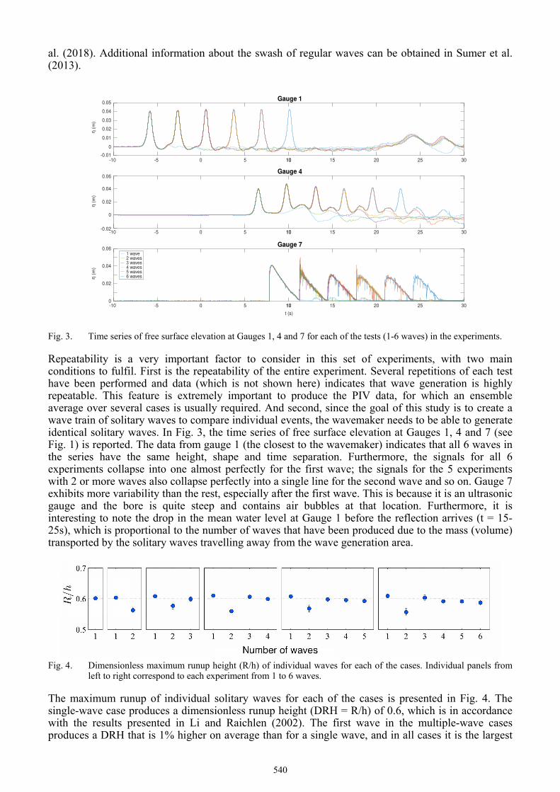
Fig. 3. Time series of free surface elevation at Gauges 1, 4 and 7 for each of the tests (1-6 waves) in the experiments.

Repeatability is a very important factor to consider in this set of experiments, with two main conditions to fulfil. First is the repeatability of the entire experiment. Several repetitions of each test have been performed and data (which is not shown here) indicates that wave generation is highly repeatable. This feature is extremely important to produce the PIV data, for which an ensemble average over several cases is usually required. And second, since the goal of this study is to create a wave train of solitary waves to compare individual events, the wavemaker needs to be able to generate identical solitary waves. In Fig. 3, the time series of free surface elevation at Gauges 1, 4 and 7 (see Fig. 1) is reported. The data from gauge 1 (the closest to the wavemaker) indicates that all 6 waves in the series have the same height, shape and time separation. Furthermore, the signals for all 6 experiments collapse into one almost perfectly for the first wave; the signals for the 5 experiments with 2 or more waves also collapse perfectly into a single line for the second wave and so on. Gauge 7 exhibits more variability than the rest, especially after the first wave. This is because it is an ultrasonic gauge and the bore is quite steep and contains air bubbles at that location. Furthermore, it is interesting to note the drop in the mean water level at Gauge 1 before the reflection arrives (t = 15-25s), which is proportional to the number of waves that have been produced due to the mass (volume) transported by the solitary waves travelling away from the wave generation area.

Fig. 4. Dimensionless maximum runup height (R/h) of individual waves for each of the cases. Individual panels from

left to right correspond to each experiment from 1 to 6 waves.

The maximum runup of individual solitary waves for each of the cases is presented in Fig. 4. The single-wave case produces a dimensionless runup height (DRH = R/h) of 0.6, which is in accordance with the results presented in Li and Raichlen (2002). The first wave in the multiple-wave cases produces a DRH that is 1% higher on average than for a single wave, and in all cases it is the largest

540

of the whole series. The second event yields the lowest overall DRH across all cases too, possibly because the second wave interacts with the first wave downrush flow, which is the strongest one, as the first wave has not undergone wave breaking during the runup phase. It can also be noted that this particular event presents slightly more variability among several repetitions than others (see variation bounds in Fig. 4). After the second wave the system reaches a quasi-steady state in terms of DRH, in which subsequent DRHs are almost constant, and just 0.8% below the initial value on average.

4.2 Numerical results

Numerical simulations are complementary to the physical experiments, as they can provide additional magnitudes with a high time and space resolution that cannot be measured in the experiments and can help to complete the dataset with cases that have not been tested physically. For this purpose, a validation stage is required, to prove that the numerical model can capture the relevant physics and flow features with the accuracy level required.

Fig. 5. Free surface elevation comparison for the 5-wave case. Experiments (blue line) and numerical model results

(3D - red line, 2D - yellow line). Gauge 2 has been selected because Gauge 1 data was used as forcing.

In order to validate the model, free surface elevation time series from the 5-wave case are presented in Fig. 5. Gauge 2 has been selected in this figure instead of Gauge 1 because the data from the latter gauge has been used as input for wave generation. As can be observed in Gauge 2, which is the closest to the wave generation boundary, the incident waves are reproduced almost perfectly (1% wave height difference), proving that the wave generation methodology explained in Section 3.2 works adequately for both 2D and 3D cases. Small differences arise after the last wave has been generated, when the reflected waves start to arrive to the gauge. These discrepancies can be attributed to two factors: the static wave generation system used in the numerical model, which does not mimic the movement of the physical wavemaker, and error accumulation in the reflected waves caused at all the stages and transformations that they have undergone. Since there are no noticeable differences between the 2D and 3D time series, we can conclude that the behavior of the flow at this location is completely two-dimensional. Gauge 4, which is located at the toe of the slope, presents noticeable deviations between the numerical simulations and the experiments. The first wave is almost perfectly reproduced, with just a minor underestimation of the wave height. The following waves, however, are slightly larger, thus, they have a higher celerity and arrive at the gauge slightly before in the numerical model. Nevertheless, the overall agreement between the signals is adequate. Moreover, 2D and 3D signals lie one on top of the other, except for small lapses of time, e.g., the crest of the second reflected wave (t = 15s). Finally, Gauge 7 is located on the swash zone. Bores run up and down this area, therefore, the profile of the waves shows a very steep front that decays progressively. As in previous cases, the first wave (nonbreaking) is reproduced perfectly by the model, both in 2D and 3D. The following waves

541

are also adequately represented, especially at the decaying part. The wave fronts tend to show more variability and significant differences between the 2D and 3D simulations, indicating that the flow in this area is highly three-dimensional, which is the case because of wave breaking.

Fig. 6. Time series of runup comparing the numerical simulations (2D and 3D) and the experiments for the 5-wave

case.

Fig. 6 shows the runup curves obtained with the numerical model in 2D (black dashed line) and 3D (red continuous line) and the maximum runup height of the experiments (horizontal blue lines, without a time reference). In the numerical simulations, the shoreline has been defined as the iso-line of 𝜎𝜎 = 0.5 at the slope. Besides, since three-dimensional effects exist in the 3D simulation, the shoreline is not uniform but presents variations in the spanwise direction, therefore, the runup height has been calculated as the median of the shoreline height. The median is used instead of the mean to prevent stuck droplets or air bubbles in contact with the slope have a major impact in the runup calculations.

The evolution of runup in Fig. 6 starts with a slight retreat from zero (theoretical shoreline at Z = 0.2m) because the resolution near the wall is high enough to reproduce the meniscus at the triple contact point (air-water-glass). Afterwards the shoreline is completely stable until waves start to arrive. Since the first wave is nonbreaking, the evolution of runup is identical in 2D and 3D, and matches perfectly the maximum runup height recorded during the experiments. Significant differences exist between the 2D and 3D simulations and the experimental results for the following waves, in which wave breaking starts playing a role. On the one hand, the 3D simulation produces a more even maximum runup height among the breaking waves, but the values are approximately 20% lower than expected. This might indicate that the turbulence model in the numerical model is dissipating more energy than in the experiments, which is a topic to investigate further in the future work. In 2D simulations the water tongue consistently reaches much higher than in 3D, which indicates that the flow loses much less energy during 2D wave breaking than in 3D simulations. This behavior was also observed and reported in Higuera et al. (2018). Moreover, the 2D results are closer to the experimental value. However, the maximum runup of the second wave is as large as for the first one.

A series of snapshots of the 3D simulation showing the interaction of the fourth wave with the downrush generated by the third wave is presented in Fig. 7. The top panel is a lateral view, in which the fifth incoming wave can be seen propagating over the constant-depth region. The right panel presents a top view of the swash zone, in which the 3D behavior of the shoreline, which is retreating at this instant, is perfectly clear. The bottom panel shows the flow velocity component in the wave propagation direction. The fast and shallow downrush flow (in dark blue) has produced flow separation and a large counterclockwise vortex can be clearly distinguished below the small overturning wave.

The incoming waves interact with the downrush flow in several stages. Initially, a small breaking event traps small pockets or air along the flume width, which are still visible in the central panel of

542

Fig. 7 (3D perspective). A second small wave breaking event occurs next. The incipient stage of this event is pictured in Fig. 7. After that, the massive momentum and mass flux of the incoming wave overcome the downrush and large-scale wave breaking occurs, trapping significant amounts of air and producing large energy dissipation. Finally, the occluded air reaches the free surface and escapes, and the runup phase continues normally.

Fig. 7. Snapshots of the 3D simulation at the instant when the fourth wave interacts with the downrush flow.

5 Conclusions and future work

In this work we have studied the evolution of a train of solitary waves, up to 6, running up and down a 1:10 slope. The evolution of the processes has been split into five different phases, including: wave generation and propagation, shoaling, runup, rundown and hydraulic jump/wave breaking, which have been described in detail. The main difference with respect to previous works, in which single solitary waves were tested, is the interaction between the wave downrush flow and the uprush of the following wave.

The experiments performed using a long-stroke wavemaker show a high degree of repeatability, both for individual waves and for the complete cases, thus allowing to collect PIV data and to compare the wave-by-wave kinematics. The experimental runup data indicates that the maximum runup height of the first wave is always the highest within each case, because it corresponds to non-breaking conditions. The second wave maximum runup is always the lowest of each case, as the second wave interacts with the most energetic downrush flow from the first wave. After the second wave, the following runup events are extremely similar and the case can be considered to have reached a quasi-steady state.

Numerical simulations have been performed with a specific wave generation methodology which does not require replicating the movement of the wavemaker and uses a time series of free surface elevation at a gauge, thus shortening the simulation domain. Validation tests based on free surface elevation time series indicate that the numerical model olaFlow is able to replicate the physical experiments with a high degree of accuracy both in 2D and 3D in terms of free surface elevation. Further analysis of the runup data, however, points out that CFD simulations need to improve in modelling the runup heights.

Future work will involve the analysis of the PIV dataset and detailed comparisons with the velocity fields obtained from the numerical model, which will possibly point out ways to improve the runup modelling.

543

Acknowledgements

The research has been supported by a grant from NRF (Singapore). The computational work was partially performed on resources of the National Supercomputing Centre, Singapore (www.nscc.sg).

References

Carvajal, M., Araya-Cornejo, C., Sepúlveda, I., Melnick, D. and Haase, J.S, 2019. Nearly-instantaneous tsunamis following the Mw 7.5 2018 Palu earthquake. Journal of Geophysical Research Letters (Accepted)

Devolder, B., Rauwoens, P. and Troch, P., 2017. Application of a buoyancy-modified k-ω SST turbulence model to simulate wave run-up around a monopile subjected to regular waves using OpenFOAM. Coastal Engineering, 125, 81-94.

Goring, D. G., 1978. Tsunamis - The propagation of long waves onto a shelf. PhD thesis of the California Institute of Technology

Higuera, P., 2018. olaFlow [Software]. http://doi.org/10.5281/zenodo.1297013 Higuera, P., Lara, J.L. and Losada, I.J., 2013a. Realistic Wave Generation and Active Wave Absorption for NavierStokes

Models. Application to OpenFOAM. Coastal Engineering, 71, 102-118. Higuera, P., Lara, J.L. and Losada, I.J., 2013b. Simulating Coastal Engineering Processes with OpenFOAM. Coastal

Engineering, 71, 119-134. Higuera, P., Liu, P. L-F., Lin, C., Wong, W-Y. and Kao, M-J., 2018. Laboratory-scale swash flows generated by a non-

breaking solitary wave on a steep slope. Journal of Fluid Mechanics, 847, 186-227. Hirt, C.W. and Nichols, B.D., 1981. Volume of fluid (VOF) method for the dynamics of free boundaries. Journal of

computational physics, 39(1), 201-225. Lee, J.J., Skjelbreia, J.E. and Raichlen, F., 1982. Measurmment of velocities in solitary waves. Journal of the Waterway

Port Coastal and Ocean Division, 108(2), 200-218. Li, Y. and Raichlen, F., 2002. Non-breaking and breaking solitary wave run-up. Journal of Fluid Mechanics, 456, 295-318. Madsen, P. A., Fuhrman, D. R., and Schäffer, H. A., 2008. On the solitary wave paradigm for tsunamis, J. Geophys. Res.,

113, C12012, doi:10.1029/2008JC004932. Sumer, B. M., Sen, M. B., Karagali, I., Ceren, B., Fredsøe, J., Sottile, M., Zilioli, L., and Fuhrman, D. R., 2011. Flow and

sediment transport induced by a plunging solitary wave, Journal of Geophysical Research, 116, C01008, doi:10.1029/2010JC006435.

Sumer, B. M., Guner, H. A. A., Hansen, N. M., Fuhrman, D. R., and Fredsøe, J., 2013. Laboratory observations of flow and sediment transport induced by plunging regular waves, Journal of Geophysical Research Oceans, 118, 6161-6182, doi:10.1002/2013JC009324.

Tadepalli, S. and Synolakis, C.E., 1994. The run-up of N-waves on sloping beaches. Proceedings of the Royal Society of London. Series A: Mathematical and Physical Sciences, 445(1923), 99-112.

544