Working Paper Augmented Simplex:

a Modified and Parallel Version of Simplex Met hod

Based on Multiple Objective and Subdifferent ial Optimization

Approach

Andrxej P. Wierxbicki

WP-93-059 October 1993

HIIASA International Institute for Applied Systems Analysis A-2361 Laxenburg o Austria

Telephone: +43 2236 715210 Telex: 079 137 iiasa a Telefax: +43 2236 71313

Augmented Simplex: a Modified and Parallel Version

of Simplex Method Based on Multiple Objective and

Subdifferent ial Optimization Approach

Andrzej P. Wierzbicki

WP-93-059 October 1993

Working Papers are interim reports on work of the International Institute for Applied Systems Analysis and have received only limited review. Views or opinions expressed herein do not necessarily represent those of the Institute or of its National Member Organizations.

HIIASA International Institute for Applied Systems Analysis A-2361 Laxenburg o Austria

Telephone: +43 2236 715210 Telex: 079 137 iiasa a Telefax: +43 2236 71313

Foreword

This initial research for this paper was performed in the Institute of Automatic Con- trol, Warsaw University of Technology, supported by the grant No. 3 0218 91 01 of the Committee for Scientific Research of the Republic of Poland. The Institute of Automatic Control has a cooperative research agreement with IIASA and the final version of this paper has been completed during the stay of the author at the Methodology of Decision Analysis Project. While based on the multiple criteria approach that has been inten- sively studied in MDA project, the paper addresses new issues of coarse-grained parallel computations.

In the perspective of parallel computations, new versions of basic optimization algo- rithms are needed. The paper presents a concept of such coarse-grained parallelization, based on a parametric imbedding into a family of problems or parametrically diversified algorithms. This general idea is exemplified for the case of the simplex algorithm of linear programming, where a linear optimization problem can be imbedded into a multiple- objective family which introduces diversified directions of search cutting through the in- terior of original admissible set. To improve the effectiveness of such algorithms, an initial phase of directional feasibility search by subdifferential optimization is added. The result- ing augmented simplex algorithm, even without parallelization, might be competitive wit#h interior point methods for a certain, broad class of linear programming problems. Neces- sary theoretical foundations, some algorithmic details and results of preliminary tests are presented.

Contents

1 Introduction. 1

2 Preliminaries. 2 2.1 Standard formats for linear simulation models. . . . . . . . . . . . . . . . . 2 2.2 Multiple-objective aspects of linear programming. . . . . . . . . . . . . . . 3

3 An augmented simplex method. 5 3.1 An augmented linear programming problem. . . . . . . . . . . . . . . . . . 5 3.2 An example of a discretized circle. . . . . . . . . . . . . . . . . . . . . . . . 7

4 Algorithmic aspects. 12 4.1 Initial feasibility phase based on subdifferentiable optimization. . . . . . . 12 4.2 A repetitive augmented simplex algorithm. . . . . . . . . . . . . . . . . . . 14 4.3 A parallel version of the augmented simplex algorithm. . . . . . . . . . . . 16

5 Conclusions. 17

A Appendices. 19 A . l A subdifferential feasibility algorithm. . . . . . . . . . . . . . . . . . . . . 19 A.2 An outline of a repetitive simplex algorithm for sequential computations. . 20 A.3 Details of parallel version of the augmented simplex algorithm. . . . . . . 22

Augmented Simplex: a Modified and Parallel Version

of Simplex Met hod Based on Multiple Objective and

Subdifferent ial Optimization Approach

Andrzej P. Wierzbicki*

1 Introduction. It is well known that the simplex method of linear programming might perform slowly

for problems with a large number of constraints, because it must go around the set of admissible solutions and cannot cut through the interior of this set. This is one of the reasons of the superiority of interior point algorithms using nonlinear penalty barrier functions (that have been also adapted for multi-objective linear programming, see e.g. Karmarkar, 1984, Arbel, 1992, Gondzio and Makowski, 1993). However, the property of searching in the interior of the admissible set is related not exclusively to the internal point methods. Some quasi-simplex or multiplier-type algorithms (see Gabasov and Kirillova, 1977, Makowski and Sosnowski, 1989) can also search through the interior. Moreover, as shown later in this paper, some formulations of multiple-objective linear programming introduce cuts through the interior even if the traditional simplex method is used. Thus, when treating an original single-objective problem a.s an example of a multi-objective one, we can improve the performance of the simplex method.

The resulting augmented simplex algorithm could be, for a certain class of problems, competitive with the internal point methods. The main advantage of the augmented simplex algorithm, however, is that it admits a natural coarse-grain parallelization which might result in a shortening of computing time as well as in an increased robustness of the algorithm for badly conditioned problems.

The perspective of parallel computing on many processors with large computing power - each well capable of solving problems of considerable size - has motivated recently many studies of parallel computations (see e.g. Nogi, 1986, Bertsekas and Tsitsiklis, 1989), in particular for linear programming (see e.g. Ruszczyfiski, 1992). Most of these studies concentrate on a decomposition of a large-scale problem in such a way that the - decomposed parts can be processed parallel - that is, on using the increased computing power for solving larger problems.

'Institute of Automatic Control, Warsaw University of Technology, Nowowiejska 15/19, 00-665 War- saw, Poland; the research reported in this paper was supported by the grant No. 3 0218 91 01 of the Committee of Scientific Research of Poland.

There might be, however, also another direction of using additional computing power in order to increase the speed and accuracy of analyzing problems of moderate scale. Since optimization is one of basic instruments in such analysis, we can expect requirements of fast and reliable execution of many repeated optimization runs, as e.g. in multi- objective decision support systems. Thus, we shall address here the question how to use future parallel computing power under the assumption that the analyzed models are not too complicated to be run in reasonable time on a single processor.

In such a case, we might use coarse grain parallelization based on a parametric imbed- ding of the original problem or algorithm into a larger family - e.g. a single-objective linear programming problem can be naturally imbedded into a related multiple-objective family - and then by coordinating the process of solving problems of this family parallel in order to obtain the solution of the original problem more quickly and robustly. This general idea of coarse-grain parallelization via parametric imbedding scheme differs in its essence from the general decomposition and coordination scheme. Moreover, this general idea applies not only for linear, but also for nonlinear or even discrete programming. However, in this paper we address only linear programming problems.

2 Preliminaries.

2.1 Standard formats for linear simulation models.

A standard form of a linear programming problem is usually written as:

where the vector x contains, beside original decision variables, also many artificial (slack) variables and thus n > m is assumed.

However, a modeler that constructs, modifies and analyses (often multi-objectively, see e.g. Wierzbicki 1992b) a linear model might find it more convenient to develop his intuitive understanding in relation to a different format that is similar to one used in (Murtagh and Saunders, 1977):

In this format, the vector x denotes only some essential or structural decision vari- ables while the vector y includes all outcome and intermediate variables used e.g. to express additional constraints. If the model is complicated, then n << m. The matrix W reflects the fact that the modeler might introduce various intermediate outcome vari- ables. Usually, (I - W)-l exists and y can be determined as a direct function of x, by substituting y = (I - W)- 'Ax and A := (I - W)- 'A; but this should be done by a preprocessing software, not by the modeler. Such a preprocessor can also perform many other transformations resulting in a simplified format similar to (I . ) :

T maximize (z = c x), X, = {x E Rn : 1 < x < U, b < y = A x < b + T E R ~ } (3)

where Int X , # 0 and lj < uj, cj > 0 V j = 1,. . . n , r; > 0 V i = 1 , . . . m might be assumed as the result of the preprocessing.

We stress that x denotes here only essential decision variables. For example, the iter- ates of an internal point method that are in the interior of the bounds on x in formulation (1) correspond rather to internal points of X, in formulation (3). The assumption that cj > 0 is made for exposition purposes only, without loss of generality.

The class of linear problems considered in this paper is such that the number n of essential decision variables is relatively small - say, comparable to the number of available processors in a parallel computer - while the number m of inequality constraints might be very large. Many practical examples and many subclasses of linear and discrete pro- gramming - e.g. semi-infinite LP - belong to this class. The selection of essential decision variables might be not unique for a given problem; although it is usually implied by the original problem formulation, we can also aggregate parts of cost function with original decision variables into new variables that can be interpreted as essential ones.

2.2 Mult iple-object ive aspects of linear programming.

Consider the following formulation of a multiple-objective linear programming problem:

where, usually, the matrix C is defined by selecting q; = y; for some 1 E j ; however, there might be several interpretations of "maximization". Generally, we can define any positive (closed, convex, pointed) cone D c R P , a corresponding strictly positive cone D and define the set of eficient solutions to (4) w.r.t. (with respect to) this cone:

xo = {x E XO : (9 + B ) U Q, = 0 where 9 = Ck, Q, = CX,), with Q, = ~ 2 , ( 5 )

If D = R:, all criteria or objectives q; are to be maximized, then by choosing D =

D \ 10) we obtain the set & of Pareto-optimal solutions, while Q, is called the Pareto frontier of the attainable objective set Q, . If we choose D = Int RP+ , then we obtain larger sets of weakly Pareto-optimal solutions and attainable objectives. The problem of finding Pareto-optimal solutions to linear programming models has been investigated extensively - see e.g. (Yu and Zeleny (1975), Gal (1977), Steuer (1986)). Most of such approaches are related to a parameterization of X, or Q, as a set of maxima of scalarizing functions, e.g. in the form of a weighted sum:

s1 (q, a) = C 0;q;

It is well known that, if a E Int R: , then all maxima of sl (Cx, a) w.r.t. x E X, are Pareto-optimal. Conversely, since X, and Q, are convex, polyhedral sets, for any Pareto-optimal q = Cx there exists an & E Int RP+ such that x maximizes s l ( C x , & ) w.r.t. x E X, .

However, there are also other cones D and D that might express various requirements of mixed maximization and minimization or even stabilization of objectives q;, and other forms of scalarizing functions that are applicable also for non-convex and discrete cases and express then the additional requirement of proper Pareto-optimality or proper eficiency

(with either bounded or even a priori bounded trade-off coefficients, see e.g. Wierzbicki, 1986, Seo and Sakawa, 1988, Lewandowski and Wierzbicki, 1989). It might seem that these other forms are not needed in the case of linear models (where all Pareto-optimal points are proper); but these alternative approaches have some desirable properties even in this case.

A general approach to the parameterization of efficient solutions is related to the following lemma (Wierzbicki, 1986, 1992a). To simplify notation, we substitute r (q ) :=

s(q, a) in this lemma.

Lemma 1 Suppose X, is compact and consider a continuous vector objective function f : Xo -+ R P , q = f (x). Given a strictly positive cone D, if a continuous function

r : R P --+ R1 is strictly monotone w.r.t. this cone (q' E q" + D + r(qt) > r(q")), then each maximum of r(f (x)) w.r.t. x E X, is eficient w.r.t. D. Conversely, if a continuous function r : R P + R1 strictly separates the sets Q, = f (X,) and 6 + D for any ij E Q, (if '(9') > 0 Vq' E 4 + D and r(qn) 5 0 Vq" E Qo ), then this property is equivalent to the three following statements:

a ) q = f (&) maximizes r (q ) w.r.t. q E Q, (& maximizes r(f (z)) w.r.t. x E Xo );

b) 4 E Q, and & E X, , they are eficient w.r.t. D;

C) r (q t ) > r(q) Vq' E 4 + D, the function r is at least locally strictly monotone.

Thus, a parameterization of Q, and X, in the sense of both sufficient and necessary conditions of efficiency might be obtained by choosing a suitably parameterized, strictly monotone scalarizing function that separates Q, and q + D. For linear models, where Q, and X, are convex polyhedral sets, the choice of the weighted sum s l (q , a) = r ( q ) might seem the most natural.

But a piece-wise linear separating function might approximate the positive cone better. A piece-wise linear function that has all the properties needed by Lemma 1 - while, not knowing in advance what is q, we use initially any q as a reference point in objective space - might be written as follows:

By maximizing this function, a Pareto-optimal point q is obtained; then the reference point q might be shifted to q. The parameter E > 0 is used in this function in order that it separates the set Q, from the cone q + Int D, , where D, is a slightly broader cone than RP+ that characterizes properly Pareto-optimal outcomes with a prior bound 1 + 1 / ~ on trade-o$ coeficients (see e.g. Wierzbicki 1986, 1992a). However, in this paper we do not need such property and thus a simpler form with E = 0 will be used:

When this function is used to characterize the set of (weakly) Pareto- optimal decisions and outcomes, then the controlling parameter of such characterization is the reference point vector q and the weighting coefficients a; > 0 play an auxiliary role. Here, however, we shall reverse the roles of these parameters; note that the weighting coefficients can

be also expressed as scaling factors or directional coefficients d; = llcr;, with d E RP interpreted as a direction of search.

If Q, and X, are convex, polyhedral sets as in (4), (5)) then the maximization of s2(Cx, q, a) over x E X, can be equivalently written as a modified linear programming problem:

max r ; XT, = {(x,r) E R"+' : x E X,, a;$ + r 5 ~ ; c ( ' ) ~ x , all i = 1 , . . . p) (7) (X,T)EX T,

where are the rows of the matrix C, q; = c ( ' )~x . This modified formulation has been used, for example, in the programming package for multiple-objective analysis and decision support DIDAS-L for linear models (see Rogowski et al., 1989; similar forms have been used earlier by many authors, see e.g. Wierzbicki, 1980, Nakayama and Sawaragi, 1983, Steuer and Choo, 1983).

The modified problem has several specific properties. Its admissible basic solutions include but are not necessarily vertices of the set X, ; its optimal solution might be any (weakly) Pareto optimal point i E % , also located on a facet or edge of the boundary of X, . This property was sometimes considered a disadvantage - see comments to a similar approach of Ecker and Kuada in Steuer, 1986 - but it is possible to use it to advantage. The modified problem might be better conditioned than the original one, since the additional constraints are orthogonal to each other. Another valuable property, observed in applications of the package DIDAS-L mentioned above, is that in certain cases the modified problem requires less simplex iterations than a comparable scalar optimization problem; this occurs because the modified formulation introduces an additional edge of the simplex that cuts through the interior of the original one.

3 An augmented simplex method.

3.1 An augmented linear programming problem.

Suppose we solve problem (3): maximize a scalar function q = cTx with respect to x E X, , and let cj > 0 for all j = 1, . . . n. Then an augmented linear programming problem can be written as:

max s , (x ,d ,x ) ; s,(x,d,x) = p T x + (1 - p ) m i n (x j - ?ij)/dj XEXo j = l , ... n

where d can be interpreted as a direction in the solution space, while dj = l/oj > 0 can be also interpreted as inverse weighting coefficients for the problem of maximizing multi-objectively all components x j as in (6b) with p = n and x j = qj ; x = q is then a reference point in the solution space.

Since cj > 0 for all j , we know (e.g. from Lemma 1) that the solution x to the original problem of maximizing cTx w.r.t. x E X, belongs to the Pareto boundary X, for the problem of maximizing all components x j multi- objectively. Thus, the augmented problem can be solved in several phases with changing coefficient p E {0,1):

an initial feasibility phase might be needed;

in the middle multi-objective phase, p = 0 until a point x E X, is found;

in the final single-objective phase, p = 1 until the solution 3i: to the original problem is found.

Note that the switch between phases corresponds only to a change of maximized function in the equivalent linear programming problem stated similarly as (7):

max (T or cTx) ; XT, = {(a , T ) E R~+' : x E X,, f j 5 xi-djr, j = 1 , . . . n ) (8b) (2 ,7)€XTO

thus the second phase can be started from the optimal basic solution of the first phase.

The properties of the augmented linear programming problem are summarized in the following Lemma.

Lemma 2 For the problem (8b) with X, defined as in (3), let c, d E Int Rn+ and denote:

IfT(x, d) n X, # 0, then for any x E T ( k , d) n X, an admissible basic solution to (8a) can be determined; in one simplex iteration, this solution can be transformed to such that maximizes T and cTx w.r.t. x E T(x,d) n X, .

Proof. Consider the way of transforming problem (8b) into the standard form (1). We add two vectors of slack variables: one for all original constraints b; 5 a i T x 5 bi + r;, s E Rm with 0 5 s 5 r, and another for additional constraints f j + d j r < f j , v E Rn with 0 5 v. Thus we obtain the set of n + m equations for 2n + m + 1 variables x, v , s , T:

Substitute x computed from the first n equations into the remaining m equations to obtain:

If x E X, , then x = x and s = s = b - A x can be selected as starting values of basic variables, with a corresponding unit basic matrix, while v = 0 and T = 0 are not in the basis. Note that T(x, d) = T(x , d) for any x E T ( x , d); therefore, if x $ X, but T(x, d) n X , # 0, we can select any x E T ( x , d) n X, and reset x := x thus obtaining an admissible starting point.

Because the method changes objective functions between phases, consider two reduced cost vectors - corresponding to these phases - at this starting point. The reduced cost vector for the multi-objective phase with maximized function T has clearly only one non- zero coordinate 1 corresponding to T. The reduced cost vector for the single-objective phase with maximized function cTx results from:

Since x and s are in the basis, the corresponding reduced cost vector is (0 0 cT ~ ~ d ) ~ . In the first iteration of the multi-objective phase, T will be selected as the variable that

enters new basis (since r is actually unbounded, it must stay in the basis in further iterations, i.e. be omitted when selecting the variables that leave the basis). The variable that leaves the basis in the first iteration is either a slack variable s; or a variable xj that first attains its bounds when x is changing along the direction d, x = x + rd - since v = 0 at the starting point.

Thus, the boundary of X, is attained in the first iteration at a point x E T ( x , d) n X, that maximizes 7; this point maximizes also cTx in T ( x , d) n X, , since cTd > 0. This concludes the proof.

Although an efficient implementation should be naturally based on an appropriate product form with good numerical stability and sparsity preservation features, the classical simplex tableau for this problem might be used to illustrate some aspects of the method. In the following tableau, two last rows represent the alternative reduced cost vectors:

Note that it is advantageous to choose x E Int X, - if x $! Int X, and x is in such boundary of X, that a further increase of r along the direction x = x + rd is impossible, then the initial basis is degenerate. Such a point is always attained after the first iteration, but with a nondegenerate basis if x E Int X, .

Such a point might not yet belong to the Pareto boundary x , since directional maximization does not necessarily imply Pareto-optimality (see e.g. Wierzbicki 1986). However, after a finite number of iterations the maximum of r in XT, will be found a t some point x, and the maximization of cTx might start from the basis corresponding to this point. The number of simplex iterations in the multi-objective phase might be very small - one, if T ( x , d) intersects X, - or large - when T ( x , d) intersects the boundary of X, far away from x,. Usually, such a point 2 is not a vertex of X, , it might belong to a facet of X, . Vertices of X, are attained after some iterations in the final single-objective phase, when continuing to maximize cTx.

Thus, the augmented simplex formulation has some similarities with interior point methods: it might start from an interior point and cut through the interior of X, in the first iteration. Additionally, since any d E Int R-might be selected, the original problem of maximizing cTx w.r.t. x E X, is em parametrically imbedded into a family of problems - or rather algorithms with parameters x, d .

3.2 An example of a discretized circle. As a way of illustrating theoretical considerations and preliminary testing more detailed algorithmic suggestions, a widely used example was selected: maximize a linear function w.r.t. x E C, , where C, is a circle approximated by many linear constraints. For example, the circle (xl -2)2 $5; 5 4 through a substitution xl = 2(1 +cosp), x2 = 2sin,B, P E [O; T] can be approximated by:

where:

while the step of changing ,B is actually 2 A p = rim. Testing results for this rather special example should be treated with care: the ad-

vantages of the augmented simplex method would be exaggerated if a very large m were chosen, hence a moderate m = 90 was selected. Additional constraints were selected as x E Bo = {x E R2 : 1 5 x 5 u), Xo = ConBo , where1 and u might be changed during various experiments with this example. In the maximized function z = cTx, c = (3 2)T was typically assumed. Thus, the problem to be solved in this example is:

maximize(qo = clxl + ~2x2); Xo = {x E R~ : x E C,, 1 5 z 5 u) XEXO

(11)

This problem was imbedded into a multi-objective family with the help of multiple- criteria decision support system DIDAS-L. This public domain software ' was slightly modified for such experiments. DIDAS-L determines automatically so called utopia points; in order to increase the freedom of experimentation, user-supplied utopia points were admitted. The simplex solver in DIDAS-L does not exploit the transformation (9b); therefore, n + 1 = 3 iterations instead of 1 iteration are needed to cut through the interior of X, . Even with this drawback, the results of preliminary experiments with this example presented in Table 1 are quite promising.

In Table 1, separate optimization means single-objective maximization of q, = cTx or of xl or x2 , and the corresponding number of simplex iterations and the optimal values

T - of xl = il , 2 2 = $2 , q, = c x are given. For the case of infeasible 1 = (0 - 2)T , the numbers of simplex iterations include the initial feasibility phase, which takes between 26 and 45 iterations; for the case of feasible 1 = (1 - l)T , no feasibility phase iterations are

Table 1. Results of experiments with augrnentedproblem, c = (3 2)x ' , u = (5 3)"

'Described shortly e.g. in Rogowski et al., 1989; full information and software can be obtained from Dr Marek Makowski a t the International Institute for Applied Systems Analysis in Laxenburg, Austria

Augmented Optim. type

Separate d l d2 9 1

Bounds max

qo 11 12 max 11

d l d z 8 2

max 2 2

d l d z 4 6

d l d 2 7 3

d l d 2 3 7

d l d 2 6 4

d l d 2 5 5

d l d n 2 8

d l d z 1 9

needed. The iterations started always from x = 1 (if they started from x = u, then 33 iterations would be needed for the maximization of go , even with feasible 1 = (1 - ). For the augmented formulation, instead of the optimal values, the values xl = Z1, x2 = 22, go = cTx after the multiple-objective phase are given in Table 1. The needed numbers of iterations are split into two parts: the iterations in the initial phase (including a possible feasibility phase) plus the iterations in the final single-ob jective phase.

Clearly, we cannot assume that we know what direction d = (dl d2)T would result in going directly from x to the optimal solution (x = (3.66 1 . 1 2 ) ~ in this case). However, some reasonable directions - such as choosing d = u - 1 (which after rescaling corresponds to d = (5 5)T in Table 1) or d = c (which corresponds to d = (6 4)T in Table I ) - result in shortening the computations more than twice. For most cases in Table 1, the total number of iterations in the augmented formulation does not exceed the number of iterations needed to maximize go separately - except in some cases, where the maximum of the scalarizing function in multi-objective phase is located on a flat part of this function, see Fig. 1. These results suggest a concept of parallelization of computations using the

Figure 1: Illustration of experiment results from Table 1. a ) Infeasible x = 1, b) Feasible x = 1.

augmented formulation. Suppose we employ a number P of processors, where P > n in this simple example. One of the processors starts to solve the original problem of maximizing go ; others solve the multiple-objective augmented problems for various d and then start the single-objective phase. The iterations in all processors are stopped if in a number of them - say, n - either the optimal solution is found or a given number tc0 of iterations of the single-objective phase is performed. This stops a large iteration; from the results obtained, estimates x and x of a relative lower bound and upper bound of the solution x of the original problem are determined. Such estimates do not serve as

modified I, u which remain unchanged, but as data used to determine the initial point in the next large iteration which starts e.g. from the new x (a relative lower bound strategy) or from the new x (a relative upper bound strategy) and possibly the directions d. This parallelization concept is rather strongly coarse-grained and thus intended either for distributed computing or for future computers with many powerful processors in a scalably parallel structure '.

For the simple example with n = 2 considered here, the way of determining a new relative lower bound estimate x is natural: just take the highest values of x j obtained from various processors which would further increase if the single-objective phase would be continued. This concept of parallelization was simulated in the DIDAS-L system (using only one processor repetitively) for the simple example of discretized circle. In the following tables, large iterations are numbered by k = 1, . . . and K denotes the number of simplex iterations (including K, = 1 additional) inside a large one. Other conditions of these experiments are as in Table 1: c = (3 2)T, u = (5 3)T, starting with (lower bound strategy) x = 1 which was either infeasible, 1 = (0 - 2)T, or feasible, 1 = (1 - I ) ~ .

The note "fail" in Table 2a means that a "processor" failed either to find optimal solution or to finish the multiple-criteria phase, thus its results were disregarded. As in Table 1, the numbers of simplex iterations needed to finish the multiple-objective phase and the values xl = Z1, x2 = Z2, q, = cTx after this phase are indicated. The first "processor" failed to find the optimal solution also in the second large iteration, but it was found by one simplex iteration of the single-objective phase in the last two "processors".

Similar experiments were performed also for P = 5, resulting in the total length of 42 iterations compared to 86 without parallelization. Note that the computational effort for coordination and communications between "processors" can be practically disregarded, since the parallelization is coarse-grained; the additional effort for coordination would be smaller than for one simplex iteration.

Table 2a. Results of simulated parallelization experiments, P=10 "processors", starting 2 = 1 = (0 - 2)T

Similar results are obtained when the experiment starts with a feasible x = 1 = (1 - I ) ~ , see Table 2b.

'The author is indebted to Dr Tatsuo Nogi from Kyoto University for stimulating discussions on future architectures of parallel computers.

Large iterat.

Total length 34 iterations, compared to 86 iterations without parallelization

Augmented Optim.

type d l d z 9 1

Separ. rnax Qo

d l d z 8 2

d l d z 7 3

d l d z 6 4

d l d z 5 5

d l d2 4 6

d l d z 3 7

d l d z 2 8

dl d2 1 9

Similar experiments with P = 5 gave total length of 12 iterations compared to 21. The speedup of decreasing the total length of computations to approximately one-half or one-third when using 5 to 10 processors is not very high. On the other hand, note that this parallelization principle produces many results that are rather close to the solution x of the original problem; this property is advantageous for badly conditioned problems ( to which belongs also the example of a discretized circle), since it increases the robustness of the algorithm. We must be prepared to pay in computational effort for this property; if we apply a rule of thumb that we consider this property equally desirable as shortening the total length of computations, we should be satisfied with a speedup close to fi.

Note that the results could be improved because n + 1 = 3 (instead of 1) iterations are used in DIDAS-L to cut through the interior of X, and the initial feasibility phase might be shortened when using the properties of the augmented formulation. However, such a simple example with n = 2 might be misleading: it is more difficult to develop a concept for parallelization if n > 2.

Table 2b. Results of simulated parallelization experiments, P=10 "processors", starting f = 1 = (1 - l )T

On the other hand, the results of this simple example justify several conclusions con- cerning possible details of an augmented simplex algorithm for larger n:

An initial phase of finding a feasible Z should be added; since Z might be any internal point of X, , methods different than in typical simplex feasibility phases should be exploited;

Large iterat.

A long final single-criteria phase might be shortened by restarting the algorithm, e.g. (when using the lower bound strategy) from a new internal x and cutting again through the interior of X,;

Total length 8 iterations, compared to 21 iterations without parallelization

Sepl max

qc

Optim type

rules for adjusting starting points, e.g. Z, and for choosing d in such repetitive augmented simplex algorithm and in its various possible parallel versions should be devised.

Augmented dl d2 9 1

dl d2 8 2

dl d2 7 3

dl d2 4 6

dl d2 6 4

dl d2 5 5

dl d2 3 7

d l d2 2 8

dl d2 1 9

4 Algorithmic aspects.

4.1 Initial feasibility phase based on subdifferentiable opti- mization.

It is well known that, instead of solving problems (3) or (8a,b), an external exact penalty function (piece-wise linear penalty terms added to the original objective function; the latter should have reverse sign to keep with the tradition of minimizing penalties) could be minimized within simple bounds I 5 x 5 u. Since such a function is subdifferentiable, an algorithm of minimizing it would consist of two interchanged operations: solving a quadratic programming problem that determines the lowest Euclidean norm element of the subdifferential and then finding a directional minimum of the function. However, such a method would usually require much more computations than the simplex method: the number of constraints in the quadratic problems, low in the beginning iterations, would gradually increase to the number of active constraints at the final solution, and the computational effort to solve each of them might be higher than when solving the problem by simplex method.

Under certain conditions, however, a subdiferentiable algorithm might be well compet- itive with the initial phase of a simplex algorithm - as long as the number of constraints in related quadratic programming problems will be low.

Consider thus the following exact penalty term:

@(x) = m,ax (max(O, b; - a('lTx) + max(0, a('lTx - bi - r ; ) ) l< t<m ( 1 2 4

Finding a feasible point means finding a minimum x of @(x) w.r.t. I 5 x 5 u such that @(x)=O. The subdifferential of @ has the form:

where:

In a typical subdifferentiable algorithm, the following quadratic programming problem would be solved:

d = argmin lld1I2 d ~ a q x )

in order to check whether a minimum is found (if d = 0) or to use d = -d in a subsequent directional search. However, there are simpler tests (e.g. @(x) = 0) to check that a minimum is found in this case and any d E -d@(x) can be used for subsequent, directional search. Thus, we shall approximate the solution of (12f) and apply a simple but effective directional search. The resulting subdiflerential feasibility phase algorithm is as follows.

Figure 2: An illustration of the subdifferential feasibility algorithm. a) full penalty approach, b) penalty term for infeasibilities.

lo Starting with given x, d and assuming x = x + ~ d , determine (similarly as when choosing a variable that leaves the basis in a simplex iteration, see Appendix 1) the values

"-u 7 71 of the coefficient T that result in satisfying either all constraints which increase along d or all constraints which decrease along d;

2' Set 7, as the arithmetic mean of T,, 71 and shift x := x + 7,d. If 71 < 7, (which indicates that T ( x , d) n Int X, # 0 and @(x) = 0) - stop.

3" Solve (12f) for an approximate subdifferential while taking into account a t most two elements -a(" or a(" that span (12b). Due to this approximation, one iteration of this algorithm requires a computational effort not exceeding the effort of one simplex iteration. Set d 2 -d, return to lo.

The algorithm is presented in more detail in Appendix 1; the main features of the algorithm are illustrated in Fig. 2.

The subdifferentiable feasibility algorithm is not always effective. If a (uniform) mea- sure of the set X, is much smaller than the measure of the set B, = {x E Rn : 1 5 x 5 u ) - see Fig. 3 - then a more standard simplex feasibility phase might be more effective, with a computational effort depending on the number of violated constraints, not on

Figure 3: The impact of the relative measure of the set X,: a) relatively large measure, b) relatively small measure.

the measures of these sets. Thus, the subdifferentiable feasibility algorithm might be used optionally in the initial phase, but it can be always used e.g. in further iterations of a repetitive augmented simplex algorithm, when an adjusted x might happen to. be infeasible.

A rough implementation of the subdifferentiable feasibility algorithm for the example of discretized circle was prepared and its results compared with the number of iterations needed for the initial phase of a standard simplex algorithm. The results are given in Table 3. Although this comparison is not quite fair - the discretized circle exaggerates the difficulties of a simplex algorithm - these results are rather striking.

I Table 2 . Comparison of standard with subdifferentiable feasibility phase

11 1 1 0 1 -3 1 -6 1 -77 1 -77 1 -77 Bounds

4.2 A repet it ive augmented simplex algorithm.

Iterations standard f. ph. Iterations subdiff. f . ph.

When starting an augmented simplex algorithm with a relative lower bound strategy, a point x situated in the middle of B, = {x E Rn : 1 5 x 5 u) might be selected,

12

211

21 2

27 1

-2 5

42 1

-5 5

45 2

-8 5

3 3 3 3 45 3

-77 23

45 4

-177 23 23

45 6

-977 23 2 3

e.g. x = 0.5(u + I). The starting direction might be either d = c or d = u - I. After correcting x by the subdifferential feasibility algorithm, we might use yet different d = x - x, where either x = u or both x and x are suitably modified after restarting the augmented simplex algorithm.

Figure 4: An illustration of a repetitive augmented simplex algorithm.

Recall that x and x denote relative lower and upper bounds for the solution x , while we know that i E X, . We shall use a heuristic supposition to estimate new and x. Suppose that a feasible x is found and the multiple-objective phase is completed at a point x E X,. The single-objective phase starts from x, but only a relatively small number of simplex iterations K, 2 2 is performed in this phase which results in another point x E x,. During these iterations, the monotonicity of changes of each variable might be tested. The supposition is that if the changes of a variable xj are monotone, they will continue to be monotone until its optimal value ij is reached. In this supposition, the concept of monotonicity might be variously interpreted: either as strict monotonicity, that each change of a variable must have the same sign, or as relaxed monotonicity, that the total change during K, iterations is much larger than the sum of changes with opposite sign.

The monotonicity supposition might be not true (imagine the surface of a sphere approximated by small triangles); therefore, we must check whether x is contained within the relative bounds x, x after K, simplex iterations of the single- objective phase and relax these bounds if needed. Even if the current solution x violates the relative bounds, we should use the available information to establish new relative bounds.

For example, if we accidentally tightened relative bounds too much, as in Fig. 3a, and obtain some z j < zj, this means that z j is essentially decreasing. We should set then Z j := z j but, at the same time, relax Z j rather strongly; we can take then Z j "all the way

through X , " - see Appendix 2 for details. The same applies to all other variables for which new estimates x are established by monotonicity supposition.

On the other hand, if the repetitive augmented simplex proceeds normally without violating relative bounds, it might give best results after new estimates for all z j are obtained by monotonicity supposition, see Fig. 3b.

The heuristic rules discussed above are summarized in an outline of a repetitive aug- mented simplex algorithm for sequential computations presented in Appendix 2. The algorithm is constructed in such a way that it is convergent in a finite number of itera- tions.

4.3 A parallel version of the augmented simplex algorithm.

For a parallel version of the augmented simplex, heuristic rules of choosing directions d are needed. If the relative lower bound strategy is used, this choice should result in possibly best estimates of the relative bounds x , while the bounds x play an auxiliary role.

It is known in the theory of multi-objective optimization that finding a precise lower bound (called sometimes a nadir point) for a Pareto set is a rather difficult computational problem. However, experience in estimating approximate bounds (e.g. in DIDAS-like systems) suggests a heuristic rule: to estimate lower bounds, reference points should be displaced along vectors m(j) = (1 . . . 1 O ( j ) 1 . . . l)T , while displacements along versors e( j) = ( 0 . . . 0 l(j) 0 . . . O)T should be used in the case of upper bounds. Clearly, { m ( j ) ) differs from {e(j)) if n > 3.

Therefore, at least 2n + 2 essential directions d(*), 11, = 1, . . .2n + 2, including d(') = c; d(2) = 5 - 2: as well as all vectors m( j ) , e(j) should be used in a parallel version of the augmented simplex algorithm (see Appendix 3 for more details).

However, in an iteration of the parallel and repetitive augmented simplex algorithm, these directions generate a cluster of points x(*) (each taken at the end of K, iterations of the single-objective phase). These points can be appropriately re-ordered according to the values of objective function. A convex combination of the best n of these results (with the highest values of the objective function) can be especially useful for generating an additional essential direction; this is a heuristic conclusion from Mazur theorem on the convergence of convex combinations. Thus (in next iterations) a preferred essential direction d(O) corresponding to such convex combination of best x(*) should be added.

Moreover, auxiliary directions d(*), 11, = 2n + 3,. . . 11,, might be useful, if they concen- trate rather closely around d(O), d('), d(2). Such auxiliary directions might be generated as convex combinations of d(O), d('), d(2) with other essential directions.

Thus, if P processors are available for parallel computations, we should choose 11,, > 3n + 2 such that X , = (11,, + 1)lP is an integer, indicating how many times a processor will be used in one large iteration - and then generate enough auxiliary directions to use fully the available processors. The times of executing an assigned number of large iterations of the repetitive augmented simplex algorithm might vary between the processors. The assignment of tasks for processors should be such that parameterized problems with more essential directions should be run first and the less preferred problems with auxiliary directions and larger 11, should be run last on all processors. We can stop then all processors a t the same time - say, when at least 11,, > 2n + 3 results x* are available - without the danger of loosing much results for more preferred directions.

The data obtained from all processors must be appropriately used for establishing new relative bounds and 5, see Appendix 3 for details. All this results in an outline of a parallel version of the augmented simplex algorithm, presented also in Appendix 3. While most discussions of this paper, for exposition purposes, concentrate on the relative lower bound strategy, it should be stressed again that a relative upper bound strategy - choosing Z as a starting point - is also possible.

A rough implementation of the repetitive augmented simplex algorithm and a sim- ulation of its parallel versions were tested on the example of discretized circle (with simplifications related to n = 2) and predictably gave better results than those presented in earlier sections; the results for relative upper bound strategy were slightly better than those for lower bound strategy. However, such results for n = 2 might be misleading; a full implementation and much more extensive testing are intended.

5 Conclusions.

A concept of a modification of the standard simplex algorithm was presented, based on an imbedding into a multiple-objective family and exploiting some ideas of subdiffer- entiable optimization and of interior point methods. The resulting repetitive augmented simplex algorithm might be competitive with interior point methods in such cases when a standard simplex algorithm would spend much time on processing consecutive vertices.

Moreover, some of the properties of this algorithm might be useful in various mod- ifications of linear programming algorithms, such as alternative initial feasibility phases or crash updates of the basis. The property of starting with any internal point and then finding vertices of the simplex might provide an alternative way of recovering a vertex solution for interior point methods, see e.g. Mehrotra (1991). However, the main advan- tage of the proposed algorithm is the possibility of its coarse-grained parallelization which might indicate a way of using future computers of scalably parallel structure.

The proposed algorithms must be yet fully implemented and extensively tested. How- ever, an early publication of these conceptual results was deemed important, since the concept of a parametric imbedding of optimization algorithms for their coarse-grained par- allelization might be also used in any other classes of problems in nonlinear and discrete optimization.

References

[I] Arbel, A. (1992) Using Sequential Generation of Anchoring Points in an Interior Mul- tiobjective Primal-Dual Linear Programming Algorithm. Working Paper of Tel-Aviv University.

[2] Bertsekas D.P. and J .N. Tsitsiklis (1989) Parallel and Distributed Computation. Pren- tice Hall, Englewood Cliffs.

[3] Gal, T. (1977) A general method of determining the set of all efficient solutions to a linear vectormaximum problem. European Journal of Operational Research, Vol. 1, No. 5, pp. 307-322.

[4] Gabasov, R. and F.M. Kiryllova (1977) Linear Programming Methods (in Russian). Isdatelstvo BGU, Minsk.

[5] Gondzio, J . and M. Makowski (1993) Solving A Class of LP Problems with a Primal- Dual Logarithmic Barrier Method. Working Paper of the International Institute for Applied Systems Analysis, WP-93-02, Laxenburg, Austria.

[6] Karmarkar, N.K. (1984) A new polynomial time algorithm for linear programming. Combinatorica, Vol. 4, pp. 373-395.

[7] Lewandowski, A. and A.P. Wierzbicki, eds. (1989) Aspiration Based Decision Support Systems. Lecture Notes in Economics and Mathematical Systems, Vol. 331, Springer- Verlag, Berlin-Heidelberg.

[8] Makowski, M. and J.S. Sosnowski (1989) Mathematical programming package HY- BRID. In A. Lewandowski and A.P. Wierzbicki, eds., op.cit.

[9] Mehrotra, S. (1991) On finding a vertex solution using interior point methods. Linear Algebra and Its Applications, Vol. 152, pp. 233-253.

[lo] Murtagh, B.A. and M.A. Saunders (1977) MINOS - a Large Scale Nonlinear Program- ming System for Problems with Linear Constraints. User Guide. Technical Report of Stanford Optimization Laboratory.

[I l l Nakayama, H. and Y. Sawaragi (1983) Satisficing trade-off method for multiobjective programming. In M. Grauer and A.P. Wierzbicki, eds.: Interactive Decision Analysis. Lecture Notes in Economics and Mathematical Systems, Vol. 229, Springer-Verlag, Berlin-Heidelberg.

[12] Nogi, T . (1986) Parallel computation. In: Patterns and Waves - Qualitative Analysis of Nonlinear Differential Equations, Studies in Mathematics and Applications Vol. 18 pp. 279-318.

[13] Rogowski T., J. Sobczyk and A.P. Wierzbicki (1989) IAC-DIDAS-L - A dynamic interactive decision analysis and support system for multicriteria analysis of linear and dynamic linear models on professional microcomputers. In A. Lewandowski and A.P. Wierzbicki, eds., op.cit.

[14] Ruszczyriski, A. (1992) An augmented Lagrangian decomposition method for block diagonal linear programming problems. Operations Research Letters, Vol. 8, pp. 287- 294.

[15] Seo, F. and M. Sakawa (1988) Multiple Criteria Decision Analysis in Regional Plan- ning: Concepts, Methods and Applications. D. Reidel, Dordrecht.

[16] Steuer, R.E. (1986) Multiple Criteria Optimization: Theory, Computation, and Ap- plication. J. Wiley & Sons, New York.

[17] Steuer, R.E. and E.V. Choo (1983) An interactive weighted Chehyshev procedure for multiple objective programming. Mathematical Programming Vol. 26, pp. 326-344.

[18] Wierzbicki, A.P. (1980) The use of reference objectives in multiobjective optimiza- tion. In G. Fandel and T. Gal, eds., Multiple Criteria Decision Making, Theory and Applications. Springer-Verlag, Heidelberg.

[19] Wierzbicki, A.P. (1986) On the completeness and constructiveness of parametric characterizations to vector optimization problems. OR-Spektrum, Vol. 8, pp. 73-87.

[20] Wierzbicki, A.P. (1992a) Multiple Criteria Games - Theory and Applications. Work- ing Paper of the International Institute for Applied Systems Analysis, WP-92-079, Laxenburg, Austria.

[21] Wierzbicki, A.P. (199213) Multi-Objective Modeling and Simulation for Decision Sup- port. Working Paper of the International Institute for Applied Systems Analysis, WP- 92-080, Laxenburg, Austria.

[22] Yu, P.L and M. Zeleny (1975) The set of all non-dominated solutions in linear cases and a multicriteria simplex method. Journal of Mathematical Analysis and Applica- tions, Vol. 49, pp. 430-468.

A Appendices.

A.l A subdifferent ial feasibility algorithm. The algorithm presented in the main text is described here in somewhat more detail:

1" Starting with given 2 , d and assuming x = 2 + r d , determine the values of the coefficient r that result in satisfying either all constraints which increase along d or all constraints which decrease along d:

rlm = rlm(Z, d) = max (Ij - zj)/dj j=l, ... n (13b)

bi - a(i)T* bi + r; - a (i)Tg ru = ru(Z, d) = min(rum, min , min ~ E I ' a(i)Td t € I U a(;)Td 1 ( 1 3 ~ )

b, - a(i)T* b; + ri - a(i)T* 71 = 7' ( 2 , d) = max(rlm, max , max

I a(i)Td i c ~ l a ( i ) T d 1 ( 1 3 4

where:

Note that ru 5 r1 indicates that T ( 2 , d) fl Int Xo = 0, but in this case a middle point between these points might be taken as an approximate directional minimum of @ ( x + r d ) .

2" Set:

where:

If 71 < 7, - which indicates that T ( x , d ) n Int X , # 0 and @ ( x ) = 0) - stop. Note that the algorithm is not stopped if 71 = 7, , because this would imply x on the boundary of X, and we can use subgradient information in such a case to find a point in the interior of X, .

3" Determine IL(x), I,"(x) as in (12c,d). Set

If 8 = 1, set d := -d(') , go to lo. Determine Euclidean norms lld(j)ll, reorder d(j) in such a way that lld(')ll 5 I ~ ~ ( ~ ) I I 5 . . . 5 lld(0)ll . Determine:

If X < 0, set X : = O . If X > 1, set X := 1. Set:

Step 3 solves approximately problem (12f). The most probable numbers of elements d(j), j = 1, . . .8 , spanning the subdifferential d@(x) in this algorithm are 8 = 1 or 2. If 8 = 1, problem (12f) is trivial. If 8 = 2, this problem is solved precisely: an element d = Xd(') + (1 - X)d(') of lowest norm, if X would not be constrained, would be orthogonal to d(') - d(2) which implies (133); because X E [O; 11, it is sufficient to project its value on this interval. If 8 > 2, the solution of (12f) is approximated by taking into account only two d(') and d@) that have the lowest norms. Due to this approximation, one iteration of this algorithm requires a computational effort not exceeding the effort of one simplex iteration.

Only the basic elements of the algorithm are presented above; they should be sup- plemented with such details as counting the number of iterations and limiting it to some reasonable value 9, - e.g. to a fraction of n + m - or projecting the directions on bounds in the case that a component x j is equal to lj or u j .

A.2 An outline of a repetitive simplex algorithm for sequential computations.

Two cases are distinguished in the algorithm: the monotonicity test is either satisfied or violated.

In the latter case, the variables that violate the relative bounds are distinguished from others. If the relative bounds are tightened too much, and some x j < zj is obtained, it is assumed that x j is essentially decreasing. Therefore, xj := x j is set and, at the same time, z j is rather strongly relaxed: it might be taken "all the way through X, " using the operation T,(x, -e(j)) defined as in (13c) with e(j) = ( 0 . . . 0 l(j) 0 . . . o ) ~ . The same applies in this case to all other variables which change monotone and for which new estimates x are established.

If monotonicity tests justify a new estimate z j after a violation of relative bounds, Z j should be strongly relaxed by taking it to uj. For variables that do not change monotone,

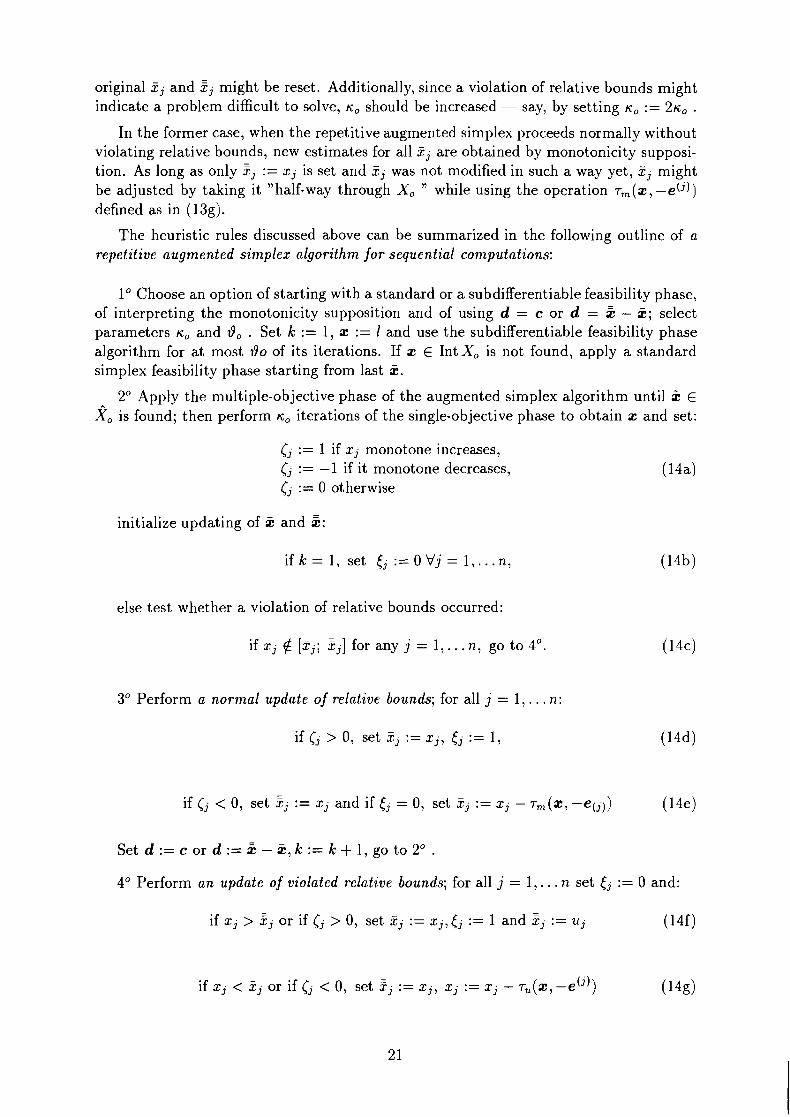
original Z j and Z j might be reset. Additionally, since a violation of relative bounds might indicate a problem difficult to solve, no should be increased - say, by setting no := 26, .

In the former case, when the repetitive augmented simplex proceeds normally without violating relative bounds, new estimates for all Z j are obtained by monotonicity supposi- tion. As long as only Z j := x j is set and Z j was not modified in such a way yet, Z j might be adjusted by taking it " half-way through Xo " while using the operation T, (2, -e(j)) defined as in (13g).

The heuristic rules discussed above can be summarized in the following outline of a repetitive augmented simplex algorithm for sequential computations:

1" Choose an option of starting with a standard or a subdifferentiable feasibility phase, of interpreting the monotonicity supposition and of using d = c or d = x - x; select parameters no and 29, . Set k := 1, x := 1 and use the subdifferentiable feasibility phase algorithm for a t most 290 of its iterations. If x E Int Xo is not found, apply a standard simplex feasibility phase starting from last x.

2" Apply the multiple-objective phase of the augmented simplex algorithm until x E x0 is found; then perform K, iterations of the single-objective phase to obtain x and set:

Cj := 1 if x j monotone increases, Cj := -1 if it monotone decreases, Cj := 0 otherwise

initialize updating of x and x:

i f k = l , set t j : = O V j = l , . . . n,

else test whether a violation of relative bounds occurred:

if x j $ [xj; xj] for any j = 1, . . . n, go t o 4 "

3" Perform a normal update of relative bounds; for all j = 1 , . . . n:

if Cj > 0, set Z j := xj, tj := 1,

if Cj < 0, set Z j := x j and if tj = 0, set sj := x j - rm(x, -e(j))

Set d := c or d := x - 2, k := k + 1, go to 2" .

4" Perform an update of violated relative bounds; for all j = 1, . . . n set tj := 0 and:

if x j > f j or if Cj > 0, set Z~ := x j , t j := 1 and f j := u j (14f)

if X j < Z j or if Cj < 0, set f j : = x j , zj := x j - ~ ~ ( x , - e ( j ) ) (14g)

else (if not (14f, g) and) if G = 0, set L j := uj, Ej := rj - ru(x, -e(j)) ( 1 4 4

Set d := c or d := x - x, k := k + 1, test whether x E Xo by performing operations (13a,. . . e) of the subdifferential feasibility phase; if not, set x := x + rl(x, d)d. Set K := 2K, go to 2".

Various details can be further specified for this outline, e.g. if a standard simplex feasibility phase is used, it might start either from I or from u; this phase should be followed by the operations (13a, . . . f ) of the subdifferentiable feasibility phase in order to obtain an 2 E Int X,. Various modifications of the rules of updating x, particularly after a violation of relative bounds, are also possible - for example, we could use more conservative updates based not on the current solution x, but on the point 37: obtained after the multi-objective phase.

Note that the algorithm is convergent in a finite number of iterations (except, in practice, badly conditioned problems for which also a standard simplex might fail): normal updates of relative bounds result in an increased effectiveness of the algorithm when compared to a standard simplex algorithm, while updates of violated bounds result in increasing K, and eventually in using standard simplex algorithm longer in the single- objective phase until the optimal solution is found.

A.3 Details of parallel version of the augmented simplex al- gorit hm.

The 2n + 2 essential directions d($) , $ = 1, . . .2n + 2 postulated for a parallel version of the augmented simplex algorithm are:

d(') = c; d(2) = 5 - 5, = rn(*-2) for $ = 3, . . . n + 2, d($) = e('+!'-n-2) for $ = n + 3,. . .2n + 2 ( 1 5 4

If such directions are used in a parallel implementation of the repetitive augmented simplex algorithm, various points ~ ( $ 1 are obtained after a large iteration of the algorithm (each taken at the end of K, iterations of the single-objective phase). Since for all ~ ( $ 1 also the values qi$) = cTx($) are known, the results can be reordered according to the decreasing values of the objective function. They will be used appropriately for updating the relative bounds 5, 2 .

However, the effectiveness of the algorithm might increase considerably if a convex combination of the best n of these results (with the highest values of the objective function) were used in next large iterations for generating an additional essential direction:

where 9, is the set of indices of n best x$ . Moreover, auxiliary directions d($), $ = 2n + 3, . . . $, are useful, if they concentrate closely around d(O), d('), d(2). Such auxiliary directions might be generated as convex combinations of d(O), d('), d(2) with other essential directions:

where X E (0; 1) is either determined or a random variable; values X close to 1 and j = 3,. . . n + 2 (corresponding to vectors m(j) that are useful for estimating 2) should be preferred. Additionally, other convex combinations (say, of all essential directions with random positive coefficients summing up to 1) might be used. It is advisable to use at least n auxiliary directions.

The directions are assigned to parallel processors as described in the main text. When stopping parallel computations after a large iteration, admissible data might come also from such processors that finished less than K , but at least 2 iterations in the single- objective phase (and thus the monotonicity indicators (! are available for each xi*)).

The data should be tested whether x(*) do not exceed the relative bounds; however, since there is more data in the parallel case, an update of violated relative bounds is needed only if, say, less than 3 best data is within the bounds. If an update of violated relative bounds is not needed, the set of indices of admissible data 9 is formed from all x* that do not violate the relative bounds; set @ is ordered then according to decreasing values of @).

In a normal update of relative bounds, if the rules (14d,e) are used to establish new bounds and many admissible data x(*) are available coming from various parts of the Pareto boundary of a polytope, various updates 2:" and d:.") (usually for different $ and $I) are obtained and a rule of choosing between them is needed. A reasonable rule is that priority is given to data corresponding to highest values of objective function (to the lowest indices of j after reordering) and to updating 2 j . Thus, 2:" and di*') are chosen that correspond to lowest indices $ and $', not such that ive e.g. the most tight bounds. These updates might be contradictory in the sense that Z b ) might be lower than

fj*'), because the supposition of monotonicity might be not true. Following the adopted

rule, the update 2; is chosen first and then a non-contradictory %I*') is selected with the possibly lowest index $I.

These rules can be summarized in the following outline of a parallel version (based on lower bound strategy) of the augmented simplex algorithm:

1" Choose an option of starting with a standard or a subdifferentiable feasibility phase, of interpreting the monotonicity supposition, parameters K , and 19, and initial x, x as in the repetitive algorithm, set k := 1. Choose integers $,, x,, $, such that:

Determine essential d(*) as in (15a) for j = 1, . . .2n + 2. Choose a rule of selecting auxiliary d(*) as in (15c) for $ = 2n + 3,. . . $, + 1 and select them. Assign to each of P processors a first direction d(*) starting with $ = 1,. . . P, then a second direction starting with lowest remaining $ etc. until each processor has X, directions assigned.

2" Run on each processor (if k= l ) the feasibility phase and (for any k) the multiple- objective phase and K , iterations of the single- objective phase of the augmented simplex algorithm for each assigned direction d(*) starting from a common 2, to obtain x(*) and the corresponding monotonicity indices (PI , j = 1, . . . n (as in the repetitive algorithm)

together with the corresponding qLi) = cTx($) . Stop if at least rl,, such data sets for various rl, are available (while accepting data from all processors that have monotonicity indicators d') available).

Initialize updating of x and X: if k = 1, set tj := 0 for all j = 1, . . . n. Determine the set Q of admissible data:

Reorder Q in such a way that qL$) 5 qLtl+') for all rl, = 1, . . . IQ I . If 19 1 < 3, determine the smallest rl, = rl,' 5 3 for which a violation of bounds x, x occurred, go to 4' .

3O Perform a normal update of relative bounds; for all j = 1, . . . n select subsequent rl, (as reordered) until:

5;') > 0; if such rl, < 191 is found, set iij := x r ) , G := 1 ( 1 6 ~ )

Then select subsequent rl, until 5;') < 0 and, if G = 1, xj') > r j ; if such rl, 5 IQI is found, set:

Zj := x(?) .I and if tj = 0, set iij := xj" - rm(x(*, -e(j)). (16d)

Go to 5O.

4' Perform a n update of violated relative bounds - for all j = 1, . . . n set tj := 0 and:

($7 if xi"') > Pj, set r j := x j , 6 := 1 and f j := uj ( 1 6 4

otherwise select subsequent rl, E 9 U {$I) and perform (16c),

or select subsequent rl, E 9 U {$I) and perform (16d) while using the operation rU instead of rm ,

Set d = c or d = x - x, k := k + 1, test whether x E Xo by performing operations (13a, . . . e) of the subdifferential feasibility phase; if not, set x := x + rl (x, d ) d . Set K O := 21c0 .

5' Set k := k + 1, 9, := 9 n (1, . . . n), n' := 19,1 and determine d(O):

Update d(2) = Z - x, reassign d(') to each processor as in lo but starting with d ( O ) , go to 2O.

Various details of this algorithm have to be modified for the case of upper bound strategy, when starting the searches from x instead of x.