histogram differences from a bar chart: bars have equal width and always touch width of bars...
TRANSCRIPT

Histogram
Differences from a bar chart:
• bars have equal width and always touch
• width of bars represents quantity
• heights of bars represent frequency
f
Measured quantity

To construct a histogram from raw data:
• Decide on the number of classes (5 to 15 is customary).
• Find a convenient class width.
• Organize the data into a frequency table.
• Find the class midpoints and the class boundaries.
• Sketch the histogram.

Finding class width
1. Compute:
classesofnumberdesiredvaluedatasmallestvaluedataestargl
2. Increase the value computed to the next highest whole number

Class Width
Raw Data:
10.2 18.7 22.3 20.0
6.3 17.8 17.1 5.0
2.4 7.9 0.3 2.5
8.5 12.5 21.4 16.5
0.4 5.2 4.1 14.3
19.5 22.5 0.0 24.7
11.4
Use 5 classes.
24.7 – 0.0
5
= 4.94
Round class width up to 5.

Frequency Table
• Determine class width.
• Create the classes. May use smallest data value as lower limit of first class and add width to get lower limit of next class.
• Tally data into classes.
• Compute midpoints for each class.
• Determine class boundaries.

Tallying the Data# of miles tally frequency
0.0 - 4.9 |||| | 6
5.0 - 9.9 |||| 5
10.0 - 14.9 |||| 4
15.0 - 19.9 |||| 5
20.0 - 24.9 |||| 5

Grouped Frequency Table
# of miles f
0.0 - 4.9 6
5.0 - 9.9 5
10.0 - 14.9 4
15.0 - 19.9 5
20.0 - 24.9 5
Class limits:
lower - upper

Computing Class Width
difference between the lower class limit of one class and the lower class
limit of the next class

# of miles f class widths
0.0 - 4.9 6 5
5.0 - 9.9 6 5
10.0 - 14.9 4 5
15.0 - 19.9 5 5
20.0 - 24.9 5 5
Finding Class Widths

Computing Class Midpoints
lower class limit + upper class limit
2

# of miles f class midpoints
0.0 - 4.9 6 2.45
5.0 - 9.9 5
10.0 - 14.9 4
15.0 - 19.9 5
20.0 - 24.9 5
Finding Class Midpoints

# of miles f class midpoints
0.0 - 4.9 6 2.45
5.0 - 9.9 5 7.45
10.0 - 14.9 4
15.0 - 19.9 5
20.0 - 24.9 5
Finding Class Midpoints

# of miles f class midpoints
0.0 - 4.9 6 2.45
5.0 - 9.9 5 7.45
10.0 - 14.9 4 12.45
15.0 - 19.9 5 17.45
20.0 - 24.9 5 22.45
Finding Class Midpoints

Class Boundaries
(Upper limit of one class + lower limit of next class)
divided by two

Finding Class Boundaries# of miles f class boundaries
0.0 - 4.9 6
5.0 - 9.9 5 4.95 - 9.95
10.0 - 14.9 4
15.0 - 19.9 5
20.0 - 24.9 5

Finding Class BoundariesFinding Class Boundaries
# of miles f class boundaries
0.0 - 4.9 6
5.0 - 9.9 5 4.95 - 9.95
10.0 - 14.9 4 9.95 - 14.95
15.0 - 19.9 5
20.0 - 24.9 5

# of miles f class boundaries
0.0 - 4.9 6
5.0 - 9.9 5 4.95 - 9.95
10.0 - 14.9 4 9.95 - 14.95
15.0 - 19.9 5 14.95 - 19.95
20.0 - 24.9 5
Finding Class Boundaries

# of miles f class boundaries
0.0 - 4.9 6 ??
5.0 - 9.9 5 4.95 - 9.95
10.0 - 14.9 4 9.95 - 14.95
15.0 - 19.9 5 14.95 - 19.95
20.0 - 24.9 5 19.95 - 24.95
Finding Class Boundaries

# of miles f class boundaries
0.0 - 4.9 6 ?? - 4.95 5.0 - 9.9 5 4.95 - 9.95
10.0 - 14.9 4 9.95 - 14.95
15.0 - 19.9 5 14.95 - 19.95
20.0 - 24.9 5 19.95 - 24.95
Finding Class Boundaries

# of miles f class boundaries
0.0 - 4.9 6 0.05 - 4.95 5.0 - 9.9 5 4.95 - 9.95
10.0 - 14.9 4 9.95 - 14.95
15.0 - 19.9 5 14.95 - 19.95
20.0 - 24.9 5 19.95 - 24.95
Finding Class Boundaries

# of miles f
0.0 - 4.9 6
5.0 - 9.9 5
10.0 - 14.9 4
15.0 - 19.9 5
20.0 - 24.9 5
Constructing the Histogram
f
| | | | | |
6
5
4
3
2
1
0
-
-
-
-
-
-
--0.05 4.95 9.95 14.95 19.95 24.95 mi.

Relative Frequency
Relative frequency =
f = class frequency
n total of all frequencies
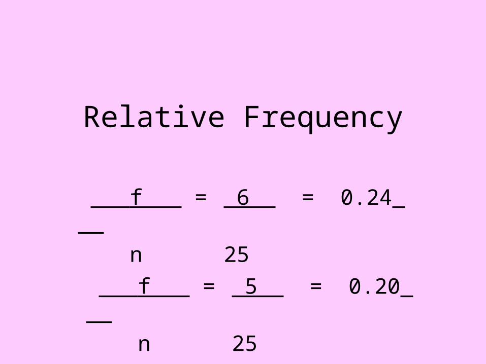
Relative Frequency
f = 6 = 0.24
n 25
f = 5 = 0.20
n 25

# of miles f relative frequency
0.0 - 4.9 6 0.24
5.0 - 9.9 5 0.20
10.0 - 14.9 4 0.16
15.0 - 19.9 5 0.20
20.0 - 24.9 5 0.20
Relative Frequency Histogram
| | | | | |
.24
.20
.16
.12
.08
.04
0
-
-
-
-
-
-
--0.05 4.95 9.95 14.95 19.95 24.95 mi.
Rel
ativ
e fr
eque
ncy
f/n

Common Shapes of HistogramsCommon Shapes of Histograms
Symmetrical
ff
When folded vertically, both sides are (more or less) the same.

Common Shapes of HistogramsCommon Shapes of Histograms
Also Symmetrical
ff

Common Shapes of Histograms
Uniform
ff

Common Shapes of HistogramsCommon Shapes of Histograms
Non-Symmetrical Histograms
These histograms are skewedskewed..

Common Shapes of HistogramsCommon Shapes of Histograms
Skewed Histograms
Skewed left Skewed right

Common Shapes of HistogramsCommon Shapes of Histograms
Bimodal
ff
The two largest rectangles are approximately equal in height and are separated by at least one class.

Frequency Polygon
A frequency polygon or line graph emphasizes the continuous rise or fall
of the frequencies.

Constructing the Frequency Polygon
• Dots are placed over the midpoints of each class.
• Dots are joined by line segments.
• Zero frequency classes are included at each end.

Weights(in pounds) f
2 - 4 6
5 - 7 5
8 - 10 4
11 - 13 5
Constructing the Frequency Polygon
f
| | | | | |
6
5
4
3
2
1
0
-
-
-
-
-
-
- 0 3 6 9 12 15
pounds

Cumulative Frequency
The sum of the frequencies for that class and all previous or later classes

Weights (in pounds) f
Greater than 1.5 20
Greater than 4.5 14
Greater than 7.5 9
Greater than 10.5 5
Greater than 13.5 0
Cumulative Frequency Table
Weights(in pounds) f
2 - 4 6
5 - 7 5
8 - 10 4
11 - 13 5
20

Ogive
Graph of a cumulative frequency table

Weights (in pounds) f
Greater than 1.5 20
Greater than 4.5 14
Greater than 7.5 9
Greater than 10.5 5
Greater than 13.5 0
Constructing the Ogive
Cu
mu
lati
ve f
req
uen
cy
| | | | | |
20
15
10
5
0
-
-
-
-
- 1.5 4.5 7.5 10.5 13.5 pounds

Exploratory Data Analysis
• A field of statistical study useful in detecting patterns and extreme data values
• Tools used include histograms and stem-and-leaf displays