SANDIA REPORTSAND2015-6368Unlimited Release

History and Evolution of the JohnsonCriteria

Tracy A. Sjaardema, Collin S. Smith, and Gabriel C. Birch

Prepared bySandia National LaboratoriesAlbuquerque, New Mexico 87185 and Livermore, California 94550

Sandia National Laboratories is a multi-program laboratory managed and operated by Sandia Corporation,a wholly owned subsidiary of Lockheed Martin Corporation, for the U.S. Department of Energy’sNational Nuclear Security Administration under contract DE-AC04-94AL85000.

Approved for public release; further dissemination unlimited.

Issued by Sandia National Laboratories, operated for the United States Department of Energyby Sandia Corporation.

NOTICE: This report was prepared as an account of work sponsored by an agency of the UnitedStates Government. Neither the United States Government, nor any agency thereof, nor anyof their employees, nor any of their contractors, subcontractors, or their employees, make anywarranty, express or implied, or assume any legal liability or responsibility for the accuracy,completeness, or usefulness of any information, apparatus, product, or process disclosed, or rep-resent that its use would not infringe privately owned rights. Reference herein to any specificcommercial product, process, or service by trade name, trademark, manufacturer, or otherwise,does not necessarily constitute or imply its endorsement, recommendation, or favoring by theUnited States Government, any agency thereof, or any of their contractors or subcontractors.The views and opinions expressed herein do not necessarily state or reflect those of the UnitedStates Government, any agency thereof, or any of their contractors.

Printed in the United States of America. This report has been reproduced directly from the bestavailable copy.

Available to DOE and DOE contractors fromU.S. Department of EnergyOffice of Scientific and Technical InformationP.O. Box 62Oak Ridge, TN 37831

Telephone: (865) 576-8401Facsimile: (865) 576-5728E-Mail: reports@adonis.osti.govOnline ordering: http://www.osti.gov/bridge

Available to the public fromU.S. Department of CommerceNational Technical Information Service5285 Port Royal RdSpringfield, VA 22161

Telephone: (800) 553-6847Facsimile: (703) 605-6900E-Mail: orders@ntis.fedworld.govOnline ordering: http://www.ntis.gov/help/ordermethods.asp?loc=7-4-0#online

DE

PA

RT

MENT OF EN

ER

GY

• • UN

IT

ED

STATES OFA

M

ER

IC

A

2

SAND2015-6368Unlimited Release

History and Evolution of the Johnson Criteria

Tracy A. SjaardemaSecurity Systems Design and Evaluation

Sandia National LaboratoriesPO Box 5800

Albuquerque, NM 87185, MS 0781tsjaard@sandia.gov

Collin S. SmithSecurity Systems Design and Evaluation

Sandia National LaboratoriesPO Box 5800

Albuquerque, NM 87185, MS 0781colsmit@sandia.gov

Gabriel C. BirchSecurity Systems Design and Evaluation

Sandia National LaboratoriesPO Box 5800

Albuquerque, NM 87185, MS 0781gcbirch@sandia.gov

Abstract

The Johnson Criteria metric calculates probability of detection of an object imaged by an optical system, and wascreated in 1958 by John Johnson. As understanding of target detection has improved, detection models have evolvedto better model additional factors such as weather, scene content, and object placement. The initial Johnson Criteria,while sufficient for technology and understanding at the time, does not accurately reflect current research into targetacquisition and technology. Even though current research shows a dependence on human factors, there appears to bea lack of testing and modeling of human variability.

3

4

Contents1 Introduction . . . . . . . . . . . . . . . . . . . . . . . . . . . . . . . . . . . . . . . . . . . . . . . . . . . . . . . . . . . . . . . . . . . . . . . . . . . . . . . . . . . . . . 7

1.1 Purpose . . . . . . . . . . . . . . . . . . . . . . . . . . . . . . . . . . . . . . . . . . . . . . . . . . . . . . . . . . . . . . . . . . . . . . . . . . . . 71.2 Background . . . . . . . . . . . . . . . . . . . . . . . . . . . . . . . . . . . . . . . . . . . . . . . . . . . . . . . . . . . . . . . . . . . . . . . . 71.3 Document Search . . . . . . . . . . . . . . . . . . . . . . . . . . . . . . . . . . . . . . . . . . . . . . . . . . . . . . . . . . . . . . . . . . . . 71.4 Summary of Findings . . . . . . . . . . . . . . . . . . . . . . . . . . . . . . . . . . . . . . . . . . . . . . . . . . . . . . . . . . . . . . . . . 7

2 History . . . . . . . . . . . . . . . . . . . . . . . . . . . . . . . . . . . . . . . . . . . . . . . . . . . . . . . . . . . . . . . . . . . . . . . . . . . . . . . . . . . . . . . . . . . 92.1 Work Prior to Johnson . . . . . . . . . . . . . . . . . . . . . . . . . . . . . . . . . . . . . . . . . . . . . . . . . . . . . . . . . . . . . . . . 92.2 Initial Validation of the Johnson Criteria . . . . . . . . . . . . . . . . . . . . . . . . . . . . . . . . . . . . . . . . . . . . . . . . . . 92.3 Extension of the Johnson Criteria . . . . . . . . . . . . . . . . . . . . . . . . . . . . . . . . . . . . . . . . . . . . . . . . . . . . . . . 102.4 Modern Challenges . . . . . . . . . . . . . . . . . . . . . . . . . . . . . . . . . . . . . . . . . . . . . . . . . . . . . . . . . . . . . . . . . . 142.5 Additional Studies and Verification . . . . . . . . . . . . . . . . . . . . . . . . . . . . . . . . . . . . . . . . . . . . . . . . . . . . . . 15

3 Factors Affecting Detection . . . . . . . . . . . . . . . . . . . . . . . . . . . . . . . . . . . . . . . . . . . . . . . . . . . . . . . . . . . . . . . . . . . . . . . . 173.1 Clutter . . . . . . . . . . . . . . . . . . . . . . . . . . . . . . . . . . . . . . . . . . . . . . . . . . . . . . . . . . . . . . . . . . . . . . . . . . . . 173.2 Signal-to-Noise Ratio and Blur . . . . . . . . . . . . . . . . . . . . . . . . . . . . . . . . . . . . . . . . . . . . . . . . . . . . . . . . . 173.3 Aspect Ratio and Viewing Angle . . . . . . . . . . . . . . . . . . . . . . . . . . . . . . . . . . . . . . . . . . . . . . . . . . . . . . . . 183.4 Visible Light vs. Infrared . . . . . . . . . . . . . . . . . . . . . . . . . . . . . . . . . . . . . . . . . . . . . . . . . . . . . . . . . . . . . . 193.5 Distinguishing Characteristics . . . . . . . . . . . . . . . . . . . . . . . . . . . . . . . . . . . . . . . . . . . . . . . . . . . . . . . . . . 193.6 Weather . . . . . . . . . . . . . . . . . . . . . . . . . . . . . . . . . . . . . . . . . . . . . . . . . . . . . . . . . . . . . . . . . . . . . . . . . . . 213.7 User Variability . . . . . . . . . . . . . . . . . . . . . . . . . . . . . . . . . . . . . . . . . . . . . . . . . . . . . . . . . . . . . . . . . . . . . 22

4 Newer Models . . . . . . . . . . . . . . . . . . . . . . . . . . . . . . . . . . . . . . . . . . . . . . . . . . . . . . . . . . . . . . . . . . . . . . . . . . . . . . . . . . . . 254.1 Triangle Orientation Discrimination . . . . . . . . . . . . . . . . . . . . . . . . . . . . . . . . . . . . . . . . . . . . . . . . . . . . . 254.2 Targeting Task Performance . . . . . . . . . . . . . . . . . . . . . . . . . . . . . . . . . . . . . . . . . . . . . . . . . . . . . . . . . . . . 254.3 ORACLE . . . . . . . . . . . . . . . . . . . . . . . . . . . . . . . . . . . . . . . . . . . . . . . . . . . . . . . . . . . . . . . . . . . . . . . . . . 264.4 Georgia Tech Vision . . . . . . . . . . . . . . . . . . . . . . . . . . . . . . . . . . . . . . . . . . . . . . . . . . . . . . . . . . . . . . . . . . 274.5 Rand/Bailey Classical Model of Search . . . . . . . . . . . . . . . . . . . . . . . . . . . . . . . . . . . . . . . . . . . . . . . . . . . 274.6 Recognition by Components (RBC) Theory . . . . . . . . . . . . . . . . . . . . . . . . . . . . . . . . . . . . . . . . . . . . . . . 284.7 Alternative Criteria for Target Dimensions . . . . . . . . . . . . . . . . . . . . . . . . . . . . . . . . . . . . . . . . . . . . . . . . 284.8 Sarnoff Visual Discrimination Model . . . . . . . . . . . . . . . . . . . . . . . . . . . . . . . . . . . . . . . . . . . . . . . . . . . . 28

5 Conclusion . . . . . . . . . . . . . . . . . . . . . . . . . . . . . . . . . . . . . . . . . . . . . . . . . . . . . . . . . . . . . . . . . . . . . . . . . . . . . . . . . . . . . . . 31

Figures1 A comparison between the ACQUIRE Model and the Johnson Criteria assuming standard N50 values

for each discrimination level. The distance difference is measured at the 50% probability of detect andcompares the difference between the Johnson Criteria and the AQUIRE Metric. These values werecalculated for a system viewing a target of 0.75 meter height, with an imaging system having a 10micron pixel and a 10 millimeter focal length. . . . . . . . . . . . . . . . . . . . . . . . . . . . . . . . . . . . . . . . . . . . . . 13

Tables1 Summary of Johnson Criteria . . . . . . . . . . . . . . . . . . . . . . . . . . . . . . . . . . . . . . . . . . . . . . . . . . . . . . . . . . 92 Variables for Calculating Probability of Detection . . . . . . . . . . . . . . . . . . . . . . . . . . . . . . . . . . . . . . . . . . 113 Variables for Time-Dependent Search Model . . . . . . . . . . . . . . . . . . . . . . . . . . . . . . . . . . . . . . . . . . . . . . 124 Summary of ACQUIRE Criteria . . . . . . . . . . . . . . . . . . . . . . . . . . . . . . . . . . . . . . . . . . . . . . . . . . . . . . . . 135 Equations for ACQUIRE-LC N50 . . . . . . . . . . . . . . . . . . . . . . . . . . . . . . . . . . . . . . . . . . . . . . . . . . . . . . . 146 Beer’s Law Atmospheric Transmission Table taken from [70, p.4] . . . . . . . . . . . . . . . . . . . . . . . . . . . . . 21

5

7 Variables for TTP Model N50 . . . . . . . . . . . . . . . . . . . . . . . . . . . . . . . . . . . . . . . . . . . . . . . . . . . . . . . . . . . 26

6

1 Introduction

1.1 Purpose

The purpose of this document is to provide a comprehensive history of the Johnson Criteria. This history containsthe work leading up to the creation of Johnson’s detection criteria, modifications applied to the criteria, perceived andactual shortcomings of the criteria, and the current status of the work being done on target detection. The shortcomingsof the Johnson Criteria are discussed in greater detail by providing the research performed on each topic between thecreation of the Johnson Criteria in 1958 up to the present day. This history is intended to clear up any misinformedideas caused by the confusion of the numerous methods and applications of target detection. An often overlookedshortcoming of the criteria is the lack of human factors or user variability data. Although minimal, the research andtesting performed on this front is also discussed.

1.2 Background

The Johnson Criteria was initially formulated as a method of predicting the probability of target discrimination. How-ever, although the simple rule that detection requires four pixels on target is remembered and used in many scenarios,the implications and required conditions of the criteria are often forgotten. This leads to misinformed decisions whendesigning and implementing target detection systems. Many factors are important when calculating the probability ofdetecting a target. These factors, their implications, proposed solutions, and research to support each of the claims aregiven for each of the shortcomings in Johnson’s original criteria.

1.3 Document Search

When researching this topic, numerous articles and reports were found. Publication dates ranged from 1948 to thepresent. These include military reports, books, and conference proceedings, among others. Some reports referencedother reports that were very difficult to find due to their either being classified, previously classified, or out of date.Much time was spent finding and reading these documents. Work was also done following given equations, applyingthem to specific situations, and attempting to verify results presented in the reports. This was sometimes difficult dueto very limited information provided by the reports themselves.

Although not an exhaustive list, the documents presented in this report cover a large majority of the reports withtopics relating to the Johnson Criteria. Over 150 papers were found and read while looking for information abouttarget detection. In total, nearly 100 documents were found that relate to the history, implementation, verification, andvalidation of, improvements to, and problems with the Johnson Criteria.

1.4 Summary of Findings

Although the detection models and metrics proposed and implemented over the last several decades have definiteimprovements over John Johnson’s original model [40], they are still lacking in a few ways. First, even thoughmany models take weather into consideration, there is still no model that accurately predicts target detection in allinclement weather situations. However, the more prevalent problem with these models is their lack of modeling of thehuman element within a detection system. Although the models take most other variables into account, the differencesbetween humans observers are not typically considered when calculating the probability of target detection. Thesemodels have included improvements to the original criteria such as taking the background, viewing angle, signal-to-noise ratio, and other factors into account when calculating the probability of target detection. It is clear that althoughtarget detection models are continuously improving, more rigorous testing is required, as is the addition of humanvariability modeling, before these models can be trusted to accurately provide the probability of target detection in anygiven situation.

7

8

2 History

2.1 Work Prior to Johnson

The foundations for target acquisition were laid down by several key researchers, not all of whom can be recognized.The work of Otto Schade in 1948 is an example of this work. His work in optics would later become the basis forJohnson’s theories on target acquisition. Otto characterized electro-optical systems and the noise associated with thesystems. [81] He also developed a metric for determining the quality of imaging systems. Other works of his includemodeling the eye a few years later in 1956, by depicting as an analog camera. [82]

The work of Albert Rose was also a basis for the work to be done by Johnson later, although his work was lesscritical. In 1948 he published a paper detailing the noise of phosphor-based illumination systems. [76] This work wasused by Johnson to describe the noise level of his system and develop an idea of the minimum detectable contrastthreshold. Johnson used this to determine the thresholds for different discrimination levels at increasing viewingdistance. [40]

Coltman studied the effects scintillation fluctuations had on the ability of observers to detect patterns on a CRT atvarying contrast levels in 1954. [15] The necessary contrast to discern bar patterns given a certain noise threshold wasof interest to Johnson due to his methodology of obtaining resolvable cycles across a target.

Dr. Robert Wiseman, Johnson’s immediate superior, also reports that Johnson collaborated with Professor HowardColeman from the University of Texas on the initial concept of equivocating resolvable line pairs and actual targets.[99] However, Coleman did not assist in this research beyond an initial intellectual level.

2.2 Initial Validation of the Johnson Criteria

The history of target acquisition generally traces its origin to the work of John Johnson in the late 1950’s. He charac-terized the probability of detecting an object based on the effective resolution of an imaged object. This is an intuitiveconcept, and one that was validated by his findings. He found that as the number of resolvable cycles across a targetincreased, so did the probability of an observer successfully locating a target. Four general categories for discriminat-ing targets were given, as shown in Table 1. This set of data, known as the Johnson Criteria, represents the number ofcycles across a target for an ensemble of observers to have a 50% chance of completing the discrimination task. [40].

Table 1: Summary of Johnson Criteria

Discrimination Level Cycles on Target DescriptionDetection 1.0±0.25 Object is of military significance

Orientation 1.4±0.35 Object aspectRecognition 4.0±0.8 Class of object (Jeep, tank, etc.)Identification 6.4±1.5 Member of class

These results were a simplification of a very complex system. Johnson recognized at the time that these numberswould change based on viewing angles and the contrast transfer function, also called the modulation transfer functionor spatial frequency response function of the system. These results were merely a way to roughly quantize the problemof detection, and were not initially expected to be used outside the Night Vision Equipment Branch. The need for sucha system, however, soon led to a wide adoption of this criteria. [99]

This concept of equivalent bar resolution became the basis of many target acquisition models for the next 50 years.The concept underlying his methodology was verified by early findings of other research groups, some of which wereunaware of his findings. The results of these experiments also showed that resolvable cycles are not the only factorsinfluencing the probability of detection.

Baker and Nicholson performed a series of studies in 1967, in which the number of scan lines across a target were

9

varied and compared against the percentage of correct responses. The targets used were Landolt C, alphanumericsymbols, and silhouettes. Unsurprisingly, it was found that as information content increased, the percentage of correctresponses increased as well. A significant result was that the number of scan lines required to recognize a silhouettevaried with the target aspect ratio and orientation. The authors conjectured that certain targets were more easilyrecognized at some angles rather than others. [5]

Erickson et al. in 1968 observed that the number of scan lines across a square would increase the percentage ofcorrect detection. This was related to the contrast of the target, but never continuously modeled. His results correctlysuggested that increase in contrast would likewise increase the percentage of correct responses. [31]

In 1969, Levine et al. measured the response times and accuracy of observers as they attempted to identify aircraftat varying resolutions and gray scale levels. They found that the performance of the observer would increase withresolution up to 12 scan lines across the target. After this, there was no significant improvement in performance. Thisindicated that modeling target acquisition as a probability was a good approach, as opposed to searching for a singleasymptotic performance level. [54]

Also in 1969, Hemingway and Erickson studied the recognition of alphanumeric symbols. At smaller angles,symbols could not be fully resolved, and performance did not reach an asymptote. Individual performance varied from50% to 97%, indicating that human factors play an important role in the probability of detection. [28]

Self published a study in 1969 detailing factors that influence target acquisition probabilities. Quantitative resultswere mentioned, but never explicitly stated. His list of qualities that affect performance include target type, size,location, and distinction from the background. He also notes that some observers in the various studies will con-sistently outperform their colleagues. He speculated that training, experience, ability, task, briefings given a priori,search habits, motivation, acceptable false detection rates, and target assumptions would all affect target detection andrecognition. [90]

In 1970, Erickson and Hemingway again published a study in which similar vehicles were identified in foliage andsand backgrounds. The results showed that observers performed better when viewing the target in foliage. [30] Thisinstance of variability due to the background was later generalized to be a function of target contrast and backgroundclutter.

Jones and Leachtenauer in 1970 classified aircrafts based on the number and type of characteristics necessary tocomplete the discrimination task. For example, the F-100’s engine intake ducts and position of the fuselage had tobe recognized by the observer to successfully identify the aircraft. [42] [52] This study showed that certain areas of atarget are more critical in identification than others.

Though noise was known to affect the probability of detection, its effects were not thoroughly modeled until 1973by Rosell and Willson. Using Johnson’s method of equivalent bar resolution and standard for a 50% probability ofsuccessfully completing the discrimination task, Rosell and Willson showed that the ability to detect a target could bemodeled as a function of SNR. [78] Others have noted that Johnson’s model tended to overestimate scenes with lowerSNR, indicating that Rosell’s ideas of SNR being related to detection probability are non-menial. [10]

In 1975, Lacey conducted an experiment which demonstrated the importance of viewing angles. A variety ofaircraft were presented to viewers at varying angles. As could be expected, targets of similar nature were morefrequently confused for each other. The ability of an observer has shown to be dependent on viewing angle. The sametype of aircraft experienced significant deviations in the percentage of correct identification when the viewing anglewas altered. [50] [52]

2.3 Extension of the Johnson Criteria

The use of the Johnson Criteria became more widely accepted, and as a result of this, in addition to an increase in thecapability of IR imaging, a surge of research began to further generalize the criteria.

In 1969, the Night Vision Lab (NVL) was attempting to develop a performance model for FLIR systems. The

10

concept of minimal resolvable temperature introduced by Lloyd and Sendall, which allowed the concept of a barresolution test to be generalized to include IR systems. Efforts were subsequently redirected to use this method tocharacterize IR systems. [98] [55]

The expansion of the criteria then took place in 1974 through the efforts of Lawson and Johnson. In this land-mark paper, several important changes surfaced. In addition to now including a metric for measuring the acquisitionprobability of infrared systems, the paper also gave an equation for relating the number of cycles across a target tothe probability of detection given the N50 of the target. These equations have evolved over time to more accuratelymodel different environments, criteria, and data sets, but the general form has remained unchanged, even in the currentTargeting Task Performance (TTP) metric. [41] [83] This is given by Equation 1. [38]

P(t) = P∞[1− e(−t/τFOV )] (1)

P∞ =(N/(N50)D)

E

1+(N/(N50)D)E (2)

E = 2.7+0.7(N/(N50)D) (3)

Table 2: Variables for Calculating Probability of Detection

Variable Unit DescriptionP(t) Unitless Probability of detection within time tP∞ Unitless Asymptotic probability; probability over infinite timeE Unitless Scaling value found from test dataN Cycles Resolvable cycles across target

(N50)D Cycles Number of cycles for 50% detectiont Seconds Time

τFOV Seconds Average time to find target

Johnson also noted that the required resolution of a target involves many factors. One of which of aspect ratioand viewing angle on target detection. He noted that objects with large widths, like ships, require different N50s thantargets such as a tank. He also noted that when viewing the same target under the same conditions from differingangles, the required resolution can vary significantly. Finally, he discussed the importance of resolving distinguishingcharacteristics, postulating that the more detailed the features were in a set, the greater the probability of detection. [22]

This work was soon expounded upon by Lawson in 1975 to make up the NVEOL model. He worked to develop aprogram to model target acquisition in which several additional parameters could be modeled. Atmospheric conditions,for instance, were being integrated into the target acquisition models. Modeling such as this had already began, but hadrecently been given a heightened interest due to problems with the current data. Navy pilots in the Mediterranean Seain 1973 found that they could detect enemy vessels at ranges greater than those predicted by the Air Force GeophysicsLaboratory. [99] This trend in modeling atmospheric data was updated in the program proposed by Lawson. It usedBeer’s law to model transitivity in a variety of weather conditions for a range of wavelengths. Though simplistic, itgave more versatility to the system’s modeling parameters. [74] [72]

In addition to adding parameters, this updated model also measured the modular transfer function (MTF) of theentire system, including the eye. This was a necessary development; because many of the previous tests in targetacquisition did not report the MTF of their system, much of the data is not applicable today. Having the MTF allowsthe data to be generalized for other systems, not just the one tested.

This model was published by Ratches the following year in 1976. It gave a succinct description of the equationsused to measure the MTF of a system, using the minimum resolvable temperature difference (MRTD), and the effectsof SNR on detection probability as measured by Rosell in 1973. This model would serve as the basis of targetacquisition modeling for the next 15 years. [72]

Erickson published another paper in 1978 attempted to incorporate the data that had been collected using scan lineson target and resolvable cycles. Realizing the importance of using metrics that incorporate a system’s ability to resolve

11

a scene, he attempted to generalize his results with that of Johnson’s. He estimated that his system had a ratio of 1.5scan lines per resolution line, or 3 per line pair, and stated that using this conversion ratio, his results were comparableto Johnson’s work in 1974. [29]

In 1978, Lawson, Cassidy, and Ratches developed a time dependent model of search, in which the probability ofdetection could be characterized by the amount of time an observer had looking at the field, as well as a function ofresolved cycles. This differed from the static approach, where observers had essentially unlimited time to detect andperform a discrimination task. [51] [73]

P = P1P2 (4)

P2 = 1− e−τ/(mt)τ =

6.8N/N50

(5)

Table 3: Variables for Time-Dependent Search Model

Variable Unit DescriptionP Unitless Total probability as a function of time and cycles on targetP1 Unitless Probability of detecting target given infinite amount of time (see Equation 1)P2 Unitless Probability of detection as a function of time given that target could be detectedm FOVs Number of sensor Field of Views within search field of regardN Cycles Resolvable cycles across target

N50 Cycles Number of cycles for 50% detection

The change from the first to the second generation of Thermal Imaging Systems (TIS) took place over the nextfew years. These imagers have a variety of differences. For instance, first-generation TIS employed raster scanning,whereas second-generations use staring arrays in two dimensions. Differences in detectors are also significant. Origi-nally, TIS generally used detectors that continually outputted a signal; a shift to on-focal-plane sampling was taken inthe latter generation where detector elements were sampled at a regular interval and then discharged for the next sam-ple. [43] Differences such as these helped to cause the need for the Static Performance Model to be updated. [38] [25]

The ACQUIRE model and FLIR90 model was developed in 1990 to work in conjunction with each other. TheFLIR90 model was an improved metric for determining the MRTD. The ACQUIRE was an improved system formodeling the probability of detecting an object. Each of these systems attempted to address several shortcomings withthe Johnson metric, as well as updating outdated metrics. These new metrics were also developed to better model thelatest generation of FLIR equipment. [75]

The FLIR90 addressed several shortcoming of the NVEOL model. [87] Firstly, it fixed the problem of varyingaspect ratios by measuring the characteristic target area in two dimensions. Noise is also modeled differently in thismodel; it is characterized in three dimensions and is divided into six categories: pixel temporal and spatial noise,temporal line and column bounce, and spatial line-to-line and column-to-column non-uniformities. The MRTD of asensor can be modeled as a function of these noise parameters, and thus can determine how noise will affect targetdetection. [86] These parameters were later expanded in the FLIR92 update. [89] Since the Ratches model of 1976was built to model first generation FLIR sensors, improvements in the physical FLIR hardware necessitated updatesfrom this previous model, thus resulting in the newer FLIR90 model. [64]

The FLIR92 model kept the majority of the parameters from the FLIR90 model. [32] An initiative led by LuanneObert and John D’Agostino addressed the noise and resolution issues of second generation FLIR systems. [73] Itadded an additional noise component of frame-to-frame noise. Improvements were made in the modeling of the eye’stemporal, vertical and horizontal spatial integration effects. This update did not change the general approach taken bythe FLIR90 model, it merely expanded it’s capabilities. This update was more widely used than FLIR90. [88] [45]

The ACQUIRE model was an improvement over the original Johnson criteria as well. It redefined some of thediscrimination categories, and, like FLIR92, it models the characteristic target dimensions in two dimensions. [32] Thenumbers of cycles for N50 were redefined to better model data and adapt to the second generation of FLIR technology

12

and to adjust for two-dimensional MRTD measurements. [75] [44] They were also generalized to match varying levelsof clutter, so that scenes with low clutter had a higher probability of detect than one with moderate clutter. The amountof clutter in a scene was subjectively assessed. [67] This metric was simplified to not measure clutter directly foreach scene, but creates general categories. The ACQUIRE model also is able to measure the probability of time-dependent detection. [27] A summary of criteria can be seen in Table 4. [91] Also, a comparison of the ACQUIREmodel to the Johnson Criteria can be seen in Figure 1. This comparison shows the probability of target detection atfour discrimination levels for both the Johnson and the ACQUIRE metrics for a range of distances. An average of theN50 values for many different targets was used in each of the metrics. The displayed distance difference measures thedifference between the Johnson Criteria and the AQUIRE Metric at the 50% probability of detect level. A negativedistance means that the Johnson Criteria predicts a shorter distance for discrimination than does the ACQUIRE Metric.

Table 4: Summary of ACQUIRE Criteria

Discrimination Level Cycles on Target DescriptionDetection 0.75 Object is of military significance

Classification 1.5 Discriminate between classes of vehiclesRecognition 3.0 Categorize within a class of similar objectsIdentification 6.0 Member of class

100 101 102 103 1040

0.2

0.4

0.6

0.8

1

Distance (m)

Prob

abili

tyof

Det

ect

Discrimincation: Detection

Distance Difference: -126.8 m

ACQUIREJohnson

100 101 102 103 1040

0.2

0.4

0.6

0.8

1

Distance (m)

Prob

abili

tyof

Det

ect

Discrimincation: Orientation

Distance Difference: 18.0 m

100 101 102 103 1040

0.2

0.4

0.6

0.8

1

Distance (m)

Prob

abili

tyof

Det

ect

Discrimincation: Identification

Distance Difference: -3.3 m

100 101 102 103 1040

0.2

0.4

0.6

0.8

1

Distance (m)

Prob

abili

tyof

Det

ect

Discrimincation: Recognition

Distance Difference: -30.0 m

Figure 1: A comparison between the ACQUIRE Model and the Johnson Criteria assuming standard N50 values foreach discrimination level. The distance difference is measured at the 50% probability of detect and compares thedifference between the Johnson Criteria and the AQUIRE Metric. These values were calculated for a system viewinga target of 0.75 meter height, with an imaging system having a 10 micron pixel and a 10 millimeter focal length.

13

There have been a number of tests that use this model, many of which have occurred recently. [24] In 1999, theACQUIRE model outperformed the FTAM model. [37] As of 2000, the US Army Materiel Systems Analysis Activitystated that the ACQUIRE model was the most accurate over a variety of conditions. [56] [3] The simplicity of themodel lends well to fitting data for a given situation, although adapting the criteria for varying situations generallyrequires experimental data. Traditionally, however, for moving targets, the N50 is 2/3 the value for an equivalent statictarget. [57] [56] The standard values of N50 are established as a basic guideline, and were modified to match newerimaging technology and to change from a one-dimensional to a two-dimensional characteristic dimension. [89]

In 2004, the ACQUIRE-LC metric was introduced to determine range for camouflaged targets. Camouflage de-velopers showed that camouflage did indeed have an impact on the range at which a target could be detected. Newequations were set to govern the type of camouflage and amount of clutter in the scene. These can be seen in Equations6 and 7.

Moderate Clutter : N50 =6

∆T 2RSS

+0.75 (6)

Low Clutter : N50 =0.75

∆T 2RSS

+0.75 (7)

∆TRSS =√(µtgt −µbkgd)2 +σ2

tgt (8)

Table 5: Equations for ACQUIRE-LC N50

Variable Unit Descriptionµtgt °K Average Target Temperature

µbkgd °K Average Background Temperatureσtgt °K Standard Deviation of Target Temperature

∆TRSS °K Target Contrast Differential Temperature

It should be noted that the equations given for ACQUIRE-LC were initially intended to only be used to detecttargets in camouflage in IR systems, but they have since been updated to apply to all targets. [47]

In 2005, the ACQUIRE and ACQUIRE-LC metrics were bound together into one metric called the Detect05. Thismodel updated clutter and adds the capability of detecting moving targets. The updated equation of clutter can be seenin Equation 9. The variables are the same as the ACQUIRE-LC model, except for C, which is a measure of clutter.For low, medium-low, medium, and high amounts of clutter, C is 1, 1.5, 2.0, and 2.7 respectively. [47]

N50 = 0.75C[(C/∆TRSS)2 +1] (9)

2.4 Modern Challenges

Understanding how modern image processing techniques affect target acquisition is just as important today as itwas when accounting for differences in imaging technology decades ago. Studies to understand the effect of videocompression on target acquisition have been an area of interest, where compression was modeled as a combinationof an MTF and blur. [14] The effects of various contrast enhancement algorithms on target detection were modeledin 2008. The increase in contrast did not significantly raise the probability of recognition. The authors speculate thatcertain critical features were not adequately resolved regardless of contrast, which significantly impacted performance.It is also important to note that the scenes were relatively clear of clutter; the contrast enhancement algorithms wouldalso cause the clutter of the scene to increase. [26] Algorithms generating super-resolved images from a series ofundersampled images can likewise be modeled by the TTP metric. [39]

14

A push for detection of targets in close-quarter situations is also underway. Urban cycle criteria are being estab-lished, in which combatants may quickly and briefly reveal themselves. [56] Recognition of the type of activities thathumans are doing are also of interest; for instance, distinguishing between pointing a rifle and using an ax is a usefuldistinction in physical security. [92] Developing criterion for recognizing objects that people are carrying are also ofinterest. [63]

2.5 Additional Studies and Verification

The Johnson Criteria is not exclusively applied to military detection - it can be used in many different applicationswhere a person is looking for a specific target in a static or moving image. The applications discussed below showother ways in which the Johnson Criteria can help in target acquisition, with targets such as guns in a public area,threats in luggage at an airport, or medical targets inside the human body.

The human factors issue is also widely relevant and applied to many different situations. As discussed in theHuman Factors section 3.7, all people are different and will see the same image differently. In order for a detectionmodel to be accurate, it must take these human differences into account. [6]

In 2000, Gale noted the similarities between image detection in medical situations and airport baggage inspection[33]. Gale discusses a training detection model developed for medical uses that has also been used in airport securitywith good success. The model is used to understand the errors involved in target detection, and thus to fix these errorsthrough different training methods. The errors possible in a target detection scenario are the same across applications,and were found to occur in the following areas: “visual search, detection of potential targets, and interpretation.”

One relevant situation is airport x-ray screening [84]. In 2005, Schwaninger et al. discuss several image basedfactors that affect threat detection in x-ray screening. These factors are view difficulty (the angle the threat object isviewed from), superposition (the amount of other objects on top of the threat object), and bag complexity (how manyother objects besides the threat object are in the bag, as well as the type of object). However, Schwaninger states thatimage based factors are not the only factors that affect threat detection. Human factors - including age, training, andvision - also affect threat detection. Schwaninger understood that threat detection could not be characterized withoutfirst characterizing the humans searching for the threat.

Another similar situation is described by Darker et al. in 2008 [18], in which the process of discovering threatdetection using closed-circuit television (CCTV) cameras can be automated. In this discussion, Darker et al. realizedthat characterizing (even minimally) the human observers (CCTV operators) in their study was an important step. Thenumber of participants, along with their gender, age, and years of experience were all reported in the paper.

Image detection is also a very important aspect in the medical field. Many medical procedures (x-rays, MRI, etc.)involve images of some sort to be taken of the body, and then examined. The entire system (from imaging device toviewing device) must provide enough resolution for medical professionals to detect problematic target areas, such asfractures in bones or growths on organs. In a report from 2005, the American Association of Physics in Medicinehighlights this dependence of medical professionals on imaging and detection techniques before going into intricatedetail about improving the imaging and viewing aspects of the process. [1].

15

16

3 Factors Affecting Detection

3.1 Clutter

Clutter is generally referred to as how complicated a scene appears. This concept, though easy to understand, hasproven fairly difficult to quantify. It is intuitive that attempting to detect a target in a plain background is much easierthan one where vegetation or other objects can obscure the initial shape of a target, as in a forest. The extraneousobjects in a scene will cause observers to not find the military target as quickly or sometimes miss it entirely. Theamount of clutter in a scene has been shown to have a significant impact on user performance, as seen in the studiessummarized below.

In his original paper in 1958, Johnson did not take clutter into account. [40] Clutter is discussed by Self in 1969.Self stated that the time it takes for a person to detect a target varied according to which background was in the image.While his definition of clutter was not thoroughly discussed, the idea of a complex background increasing the difficultyof detection was noted. [90]

Erickson and Hemingway studied similar situations a year later in 1970. Their experiments showed that thepercentage of observers who were able to successfully detect a target in foliage was roughly 20% higher than on asandy background. [30] This was significant, especially since the factors that affect scene detection were still beingmodeled. [78]

In 1983, Schmieder and Weathersby derived a clutter metric by measuring the standard variation of the radiancein a scene. They noted that clutter and time-varying noise are not equivalent phenomena. They also experimentallyshowed that as clutter levels increased, the number of cycles required to resolve a target also increased. For sceneswith low clutter, for 50% probability of detection, N50 was 0.5 and for high clutter it was raised to 2.5. [83]

Research done by Georgia Tech Research Institute has attempted to quantify the effects of various parameters onclutter level. They also presented a new metric of clutter, which defines a pixel-by-pixel definition of scene complexity.Parameters such as air temperature, solar irradiance and time, mean temperature, and wavelength for data collectionwere correlated with clutter to determine which, if any, external parameter affected the clutter level of the image.General trends were established, such as an increase in clutter with the time of day, but the scatter for the fitted lineswas large. [35]

Mazz agrees with the correlation between the complexity of a scene and the difficulty of locating an object in1998 by stating that as clutter increases, the N50 values for IR also increase. Images were subjectively sorted into fourcategories and their N50 values compared. The cycles required for detection varied from 1.3 to 2.5 cycles. It is alsointeresting to note that as clutter increased, so did the false detection percentage (FDP). He postulates that the effectof clutter and FDP are additive. [57]

In 1999, Horrigan pointed out that it becomes very difficult to attempt to model clutter. Many parameters can resultin many complicated equations. He attempts to cover some shortcomings of the ACQUIRE model and standardize thevariations of the clutter metrics presented in past years. His model, the FLIR Target Acquisition Model, was not assuccessful as the ACQUIRE model, however. [37]

Research done by Bhanu and Rong from the University of California has resulted in methods to model the clutterof the background of a scene. This was done to make automatic target detection possible while reducing false alarms.The process of target detection includes selecting all potential target areas, then comparing these against modeledbackgrounds in order to filter out any false alarms. [7]

3.2 Signal-to-Noise Ratio and Blur

Signal-to-noise ratio (SNR) factors into the ability to detect targets. Blur affects object recognition in a similar way.Both are concerned with the quality of image. Noise and blur were of concern when evaluating the quality of an image,

17

dating back to Schade’s work in the 1940’s. Blur affects the quality of an image even with modern optical systemsand is now measured by an MTF; an optical system may not be able to sufficiently focus the scene due to inherentaberrations in the lenses, thereby spreading the light to neighboring pixels, causing blur.

In 1969, Self noted that a noisy image affected object detection, but he never quantified this result. He also notedthat the sharpness of an image was related to observer performance. [90]

Also in 1970, Scott, Hollanda, and Harabedian all tested the effects of SNR with respect to scan lines required toresolve a target. [85]

A significant contribution to the field of target acquisition came from Rosell and Wilson. Through a series ofpapers, they related the ability of an observer to detect an object to the SNR of the image. [79] [77]

In 1974, O’Neill saw that ships with the same resolution had different levels of detectability under varying levelsof SNR. [2] [69]

In 1981, Burke showed that blur and noise are interrelated. Air Force photo-interpreters qualitatively ranked theinterpretability of 250 military scenes. The study reported that adding noise to a blurry image did not affect judgmentnearly as much as adding blur to a noisy image. [13]

Similarly, in 1983, Politte, Holmes, and Snyder noticed that blur and noise resulted in reduced judgment of imagequality. He also noted that as SNR decreased, the effects of other variables of observer variability decreased aswell. [2] [71]

In 1997, Aleva and Kuperman note that the effects of blur and noise together are much more detrimental than whentaken separately. This is apparent in the ROC curves published in the original report. As expected, as noise and blurincreased, observer performance decreased. [2]

Mazz analyzed the variability in N50 in 1998, and showed that sensor resolution was inversely proportional to thecycles on target required for detection. The author also notes that this correlation was confounded by the fact that thefalse detection rate also decreases in this experiment. [57]

Using the ACQUIRE model in 2007, Krapels and Driggers saw that the probability of detection decreased as blurincreased. This is because they showed experimentally that a blurred image contained fewer resolvable cycles than itsunblurred counterpart. [46]

In 2008, a study on the cycle criteria required to resolve thalassic vessels used blur to simulate a decrease inresolvable cycles on target. The MTF of the blur was able to be mathematically modeled, and thusly incorperated intothe system MTF. The TTP metric was able to predict the decrease in performance based on the change in MTF. [48]

3.3 Aspect Ratio and Viewing Angle

A target may appear different depending on the angle for which it is viewed. Johnson’s original criteria assumed thatthe target would carry information necessary for discriminating between different targets. This is not always true,especially for similar objects. It is also not true that the entirety of an object’s area carries discriminating information.The probability of discrimination is related to an object’s aspect ratio and the viewing angle. Aspect ratio is the ratioof the height of the object to the width. Viewing angle refers to the orientation of the object.

In 1972, it was first realized that the angle at which the object was viewed greatly impacted the way an objected wasseen. It was Moser who noticed that the Johnson Criteria did not hold true for Naval vessels at certain aspect angles,suggesting that the side view would be much more useful than the bow view. He noted that the ratio of dimensions ofa single target varied from 1.2 to 14.6 depending on the angle for which it was viewed and that not all of the resolvedarea was pertinent to discriminating between types of targets. He instead suggested using the perimeter of the ship asa measure of information content. [62]

18

Only a few years later in 1974, Johnson and Lawson showed that the number of cycles required for target discrimi-nation varied significantly with changes in viewing angle for objects with a large aspect ratio. [41] Ratches noted in theStatic Performance Model that the cycle criterion given had been averaged over a myriad of targets and orientations.He noted that targets with aspect ratios in great excess of one will deviate from these significantly. [74]

The variations of performance based on target orientation is a well understood phenomenon. It is casually takeninto consideration in studies where aspect ration and viewing angle are not the main topic of interest. In 1991, Rotman,Gordon, and Kowalczyk studied how varying the density of smoke would affect target detection. They showed that atank would have a much higher chance of being detected, over 30% better chance, if viewed from the side rather thanthe front. [80]

In 2001, Leachtenauer noted that the percentage of correct identification of aircrafts varied as much as 60% whenviewing the same target from different angles. [52] This study also indicates the effect of viewing angle is correlatednot only with the size of the target, but the distinguishing characteristics available to the observer.

3.4 Visible Light vs. Infrared

When dealing with probability of detection, there are many differences when using visible systems versus infrared(IR) systems. These differences include the times and situations during which each are best used, the operation ofthe cameras used for detecting images of each type, and the detail shown by the resulting images. Weather is a largedeciding factor for deciding between using a visible or an infrared system, as fog obscures visible systems more thaninfrared systems.

In 1994, Howe discussed the current status of modeling IR systems, as well as future challenges to face. In this hediscussed some of the problems associated with imaging with FLIR technology. The strongest problem involved targetboundaries blending into the background of a scene. Howe discussed how the current version of thermal models failedin this area, as well as in situations where the target was highly cued. These difficulties do not show up as strongly invisible systems. [38]

The variability in N50 was also noted when comparing IR and visible data sets. A report released in 1998 showedthat the detection N50 ranged from 0.75 to 4.1 cycles on target required for detection with an average of 1.8 ± 0.93for the 24 tests reported. It should be noted that the highest variation of 13.7 cycles was excluded from analysis dueto uncertainty in the MRTD during acquisition. For visible data sets, cycles varied from 0.72 to 11.7 cycles on targetwith an average of 4.58± 3.45 for a total of 8 tests reported in the report. These tests were done with varying numbersof observers, target types, time of day, time limits, target opportunities, location, clutter, and ranges. [57]

O’Connor also noticed, in 2003, a difference between probability of detect between visible and IR systems. Theprobability of detect was greater in the visible spectrum than in the IR. The N50 values for visible systems weremeasured to be 7.5 while the IR system was 11.5. He speculates that the removal of details, such as paint color,explains why the visible system outperformed the IR system. [65]

In 2008, small watercraft cycle criteria were developed for the ACQUIRE and TTP metrics for SWIR systems.Blur was added to decrease the cycles on target for each image, and each vessel was filmed from 12 different angles.Data was compared to a previous data set for similar type of crafts which were imaged in the MWIR and visible range.The characteristic dimension of the crafts for the two tests were recorded as 3.9 meters. The N50 for the visible set(recorded in grayscale) was 4.0, as compared to the MWIR and SWIR, which were 2.8 and 3.5 respectively. The V50for visible, MWIR, and SWIR are 14.0, 10.6, and 11.3 respectively. [48]

3.5 Distinguishing Characteristics

Object identification has been shown to depend greatly on the ability to resolve distinguishing characteristics. Thisconcept has important implications in target acquisition. The ability to view these characteristics are assumed to be

19

true in the ACQUIRE and TTP metrics; if this assumption is not true, the performance of the system risks severedegradation.

Moser, in 1972, noted that he perimeter of an object might be a better metric to assist in predicting target acquisitionperformance. He showed that the Johnson Criteria did not apply to some naval targets, and noted that most of thearea of a ship is featureless, and will not assist in target recognition. He conjectured, “Perhaps a better measureof information content would be the resolvable perimeter of the target or the number of resolvable angles along itsperimeter.” [62]

Johnson first documented in 1974 that, “Recognition probability is determined by the perception of target features.”Johnson continues to explain that more features and detailed features would lead to increased probability of detect.[22] [41]

One of the major theories that attempts to model how humans recognize objects was developed by Biederman in1987. He attempts to classify objects as being comprised of simplified subsections called “geons.” [8]

O’Kane, Biederman, and Cooper analyzed the correlation of critical features and target recognition in 1996. De-veloping a dichotomous decision tree for target recognition, they showed that the percentage of confusion was highlycorrelated with the nodal separation on the decision tree. It was then shown that the ability to detect critical featurecorrelated with the variance in observer performance more so than physical phenomena, such as range, target size,and atmospheric transmission. [80] It should be remembered that the physics-based ACQUIRE model predicts theperformance of an ensemble of observers, not individuals.

In 1997, O’Kane predicted that object confusion could be modeled. O’Kane noted that visual misidentificationwas a significant problem by relating Herdman’s research in 1993 that “15% - 20% of US Army casualties have beenestimated to be cases of fratricide,” [34] showing a strong need to reduce the occurrence of such misidentification.This led O’Kane to conduct experiments from which predictions of detection could be made from the number ofdistinguishing features on vehicles. This could greatly improve identification models. [66]

In 2001, Leachtenauer noticed that military targets with similar features were more often confused with each other.For example, identical engine intakes on aircrafts led to a higher percentage of misidentification. The features requiredto detect a variety of aircraft and terrestrial vehicles were analyzed. [52]

Similarly, in 2003, O’Conner measured the N50 of 12 different tanks. These tests were performed without fueldrums, erected radars, etc. He showed that the removal of these “giveaway” target identification tags increased thedifficulty of detection. [65]

That same year, Leachtenauer published a paper detailing a brief history of models based on the Johnson Criteriaand stressed the importance of recognizable characteristics. He emphasized knowing what direction the enemy wouldlikely approach from, and encouraged cycle criterion to be based on that orientation. [53]

In 2008, Darker et al. in the United Kingdom began to research how CCTV operators detected people carryingconcealed and unconcealed firearms in public places. Through surveys, Darker and team were able to make up a listof most-used operator strategies for detecting firearms. This study shows how certain characteristics allow for easierthreat detection, and provides confirmation as to the importance of discernible target features. [18]

The question of how best to detect an object in an image is relevant to many different applications, including airportsecurity bag checks. In 2008, Schwaninger et al. discussed the factors that affect threat detection in X-ray screening.Several image based factors were defined, including view difficulty, superposition, clutter, and opacity. [11]

In 2013, Maurer et al. discusses image-based modeling, noting that in 2001, NVESD began to develop image-based models. Image-based modeling uses details of the image to give predictions of target discrimination. [56]

20

3.6 Weather

Weather conditions can greatly impact the probability of detect. Most studies have been performed with fog or smoke,for both visible and IR cameras. Work done on calculating how the vision-obscuring smoke and fog affects detectionis important, especially for naval purposes on the coast. However, although much research has been done on thequalitative effects of fog and smoke, not much research has been performed quantitatively. For example, “heavy fog”is quite an arbitrary definition. A much better description would take into account the number and size of the particlesin the air. Since this research is much more work-intensive, it is not often done. However, the results taken fromrelatively well-defined qualitative data provides a foundation for understanding the effects of particles in the air ontarget detection.

Beginning in 1975, Ratches and Lawson reported results from the experiments they performed with fog. Theymodeled the transmission of light through fog for a detection system using signal-to-noise ratios between the targetand the fog, respectively. This model had an accuracy of ±20% when testing the optimum situation. However, thereare few results from field tests due to the dynamic nature of fog. Even so, it is clear that testing in inclement weatheror with difficult targets greatly degrades the results. At the time, work was being done to improve the model for theseadverse conditions. [74]

Over 15 years later, in 1991, Rotman, Gordon, and Kowalczyk performed experiments with smoke. They noticedthat obscurants are not a constant source of interference; there are natural fluctuations in the density of the smoke orfog. This was tested in simulations where the ability to detect a tank in constant and fluctuating levels of the smokewas measured as a function of time over a variety of wavelengths. It was found that the probability of detection influctuating obscurants is generally higher than if it were constant. [80]

Krapels et al. published a study in 2001 to determine the feasibility of modeling turbulence as an MTF. TheNVESD studied a similar model produced by researchers at Ben-Gurion University. Krapels et al. evaluate this MTFmodel, and conclude that it is a viable model and reasonable to use in the model for the US Army. [49]

The ability to model atmospheric degradation through computer simulations have been in use since the 1970’s,which started with LOWTRAN. The database has been updated through the years and is now called MODTRAN.NVThermIP is able to model atmospheric effects. It can be done through MODTRAN, Beer’s law, or an input table.

The ability to model atmospheric effects is important, as shown by Table 6. The probability of detection dropssignificantly as the average transmission over 10 kilometers, τ(ave), decreases, especially at longer distances. Thesenumbers do not accurately describe the real world, as the model is much more complex than used here. However, theydo show how severely adverse weather conditions affect the probability of detection, and emphasize the importance ofmodeling weather conditions when looking at the probability of detection. [70]

Table 6: Beer’s Law Atmospheric TransmissionTable taken from [70, p.4]

P(det)Range (m) τ(ave) = 100% τ(ave) = 50% τ(ave) = 25% τ(ave) = 10%

0 1 1 1 11 1 1 1 13 0.999 0.998 0.996 0.9915 0.982 0.963 0.934 0.8747 0.938 0.878 0.792 0.6449 0.878 0.765 0.620 0.41210 0.845 0.706 0.537 0.315

21

3.7 User Variability

User variability and human factors are topics which are lacking in the literature of imaging criteria. Some papers notethis lack of information whereas others ignore it all together. However, no paper ever attempts to completely modelhuman factors or user variability, nor have experiments been performed to completely characterize variability betweenobservers. This is an important part in defining probability of detect, and must be taken into account in order to givevalidity to the model.

In 1969, Self gave a list of studied observer traits and behaviors that were relevant to predicting probability ofdetect. These behaviors included using several different search patterns to search the images. The relevant traitsincluded the amount of training and instruction the observer had received and the amount of pressure the observer wasunder.

Self also discusses observations he made about searchers. These include over-searching likely areas while ignoringothers, rapidly searching likely areas rather than searching the entire scene systematically, and forgetting to searchcertain areas of a scene. Results of these search patterns include not quickly finding a target in an unlikely area,finding a target in the center of a scene more quickly than targets on the edges, and, as expected, not quickly finding atarget in forgotten areas of the scene. Also, observers who were under pressure more quickly found targets than thoseunder no pressure. Lastly, Self observed that chance played a large part in detecting targets. [90]

In 1991, Donohue states that Johnson ignored variability between observers when discussing factors that influ-ence target detection. Donohue confirmed Self’s predictions that an observers’ training, experience, native ability,instruction, briefing, motivation, compromise (speed vs. accuracy), and assumptions all affected the performance ofobservers. [22]

In 1994, Miller surveyed a group of soldiers about factors they believed to be important in target acquisition. Theseincluded threat level, combat experience, training, stress level, etc. The soldiers qualitatively designated importanceto each of these factors that they believed to be important. Later, the same test was administered asking the samequestions. The results from the two surveys varied significantly, indicating that the question of human factors cannotbe quantified by consulting field users. Instead, he developed a fuzzy logic model for the JANUS target acquisitionsystem. [61]

Soon after, in 1995, Valeton and Bijl conducted experiments on human performance on target acquisition. Partof the purpose of these experiments were to validate the TARGAC model. One of their conclusions was that militaryobservers were more likely to react to a stimulus whereas civilians tended to wait until they were certain. This adds tothe idea that training impacts performance. [94]

Mazz compiled a report showing that, although models like ACQUIRE are able to predict the performance of anensemble of observers, the performance of individuals in the group can vary widely. A Monte Carlo simulation wasrun to generate statistically equivalent observers and compared to the results gathered from war game simulations.The spread of probabilities for any given averaged probability was much smaller in the simulation than for an actualobserver. This indicates that factors other than expected statistical variations cause observer scores to vary. [58]

In 1999, Ratches, while discussing the MRTD model, mentioned that the model depended on both sensor andobserver variables. The model takes observer eye integration time into account, but Ratches notes that althoughtraining, motivation, and reward also affect detection, these factors have not been incorporated into the MRTD model.[73]

In 2008, Bolfing noted the importance of quantifying the human observers used in his test on detection of airportthreats. The study recorded the gender, age range of the observers, and hours of training for each observer, andreported results as they correlated with these factors. Bolfing showed that age had a smaller yet noticeable affecton target detection. When comparing the affect of all these human factors on threat detection, a regression analysisgives an R2 value of .69, showing a noticeable correlation. Further analysis shows this correlation is statisticallysignificant. [12]

According to Maurer, many factors affect search and detection models, one of which is variations between ob-

22

servers. As recently as 2013, Maurer notes that work is still being done to improve these models, and that this work isrequired in order to modify and improve these models. Although the models give reasonable results now, as technologyimproves, the models of target detection will improve as well. [56]

23

24

4 Newer Models

In order to better keep up with the development of imaging technology and improved understanding of the humanpsychophysiology, newer metrics have been proposed. Some have been accepted and widely implemented, and othersare still competing for a clear superior system.

When testing new models, the Army has determined that predicting the performance of a model includes validating,verifying, and accrediting the model. Validating includes comparing the results of experiments with the predictionsgiven by the model. Verifying involves making sure the model’s equations concur with the physics of the scenario andsystem, and accurately representing these equations in code. The last step of accreditation consists of noting the typesof situations in which the model works. [60]

4.1 Triangle Orientation Discrimination

The Triangle Orientation Discrimination (TOD) threshold is a metric that was proposed to modernize the charac-terization of electro-optical system performance. It claims that the old metrics of minimum resolvable temperaturedifference (MRTD) and minimum resolvable contrast (MRC) are limited in several areas. Only the amplitude is takeninto account when viewing the bar pattern, which means that the spatial phase spectrum is ignored, even though it con-tains potentially useful information. Aliasing effects also occur when bar patterns with frequencies greater than theNyquist frequency of the imaging system is used. A lack of standardization in testing also produces some ambiguityin these results. [9]

Instead, the TOD presents triangles to observers and asks them to distinguish their position and orientation. Thismethod has several advantages. It is applicable to many types of imaging systems, including both IR and visible. It canalso be used by the ACQUIRE model. [9] Determining the best metric to evaluate sensor performance is not clearlydefined as of yet. [39]

4.2 Targeting Task Performance

The most recent metric proposed by the NVESD is the Targeting Task Performance (TTP) metric. This metric attemptsto address some of the inherent flaws in the Johnson criteria as it relates to modern technology, such as the use of focalplane array imagers, and human psychophysics, such as the Contrast Transfer Function (CTF) of the eye. [96] [97]The CTF accounts for the fact that humans are able to discern details at lower levels of contrast better at certainspatial frequencies than at others. This metric also explicitly takes into account the probability of detection by chance,something that is not always done in the Johnson-based models. If an observer reports whether an object is of militaryimportance, he will be correct 50% of the time by pure chance. This model also keeps with previous methods ofaccounting for target size and aspect ratio by characterizing its dimensions as the square root of the area.

Ctgt =

√∆µ2

tgt +σ2tgt

2µbkgd(10)

V =∫

ξcuto f f

ξcuton

√Ctgt

CT Fsys(ξ )

Atgt

Rdξ (11)

N = ξcuto f fAtgt

R(12)

P =

(V

V50

)β

1+(

VV50

)ββ = 1.51+0.24

VV50

(13)

25

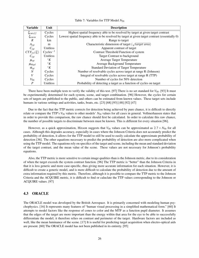
Table 7: Variables for TTP Model N50

Variable Unit Descriptionξcuto f f Cycles Highest spatial frequency able to be resolved by target at given target contrastξcuton Cycles Lowest spatial frequency able to be resolved by target at given target contrast (essentially 0)

R km Range to targetAtgt m Characteristic dimension of target (

√target area)

Ctgt Unitless Apparent contrast of targetCT Fsys(ξ ) Cycles−1 Contrast Threshold Function of system

Ctgt Unitless Target Contrast to backgroundµtgt °K Average Target Temperature

µbkgd °K Average Background Temperatureσtgt °K Standard Deviation of Target TemperatureN Cycles Number of resolvable cycles across target at range R (Johnson)V Cycles Integral of resolvable cycles across target at range R (TTP)

V50 Cycles Number of cycles for 50% detectionP Unitless Probability of detecting a target as a function of cycles on target

There have been multiple tests to verify the validity of this test. [97] There is no set standard for V50. [93] It mustbe experimentally determined for each system, scene, and target combination. [96] However, the cycles for certainsets of targets are published to the public, and others can be estimated from known values. These target sets includehumans in various settings and activities, tanks, boats, etc. [23] [68] [93] [48] [92] [47]

Due to the fact that the TTP metric corrects for detection being achieved by pure chance, it is difficult to directlyrelate or compare the TTP’s V50 values to other models’ N50 values for all cases in general. Vollmerhausen states thatin order to provide this comparison, the raw chance should first be calculated. In order to calculate this raw chance,the number of possible targets to discriminate between must be known. This is different for every situation [96].

However, as a quick approximation, Hixson suggests that V50 values can be approximated as 2.7×N50 for allcases. Although this degrades accuracy, especially in cases where the Johnson Criteria does not accurately predict theprobability of detection, it allows for the TTP model to still be used to easily calculate the approximate probability ofdetection [36]. The other equations necessary to predict the probability of detection are also more complicated whenusing the TTP model. The equations rely on specifics of the target and scene, including the mean and standard deviationof the target contrast, and the mean value of the scene. These values are not necessary for Johnson’s probabilityequations.

Also, the TTP metric is more sensitive to certain image qualities than is the Johnson metric, due to its considerationof when the target exceeds the system contrast function. [96] The TTP metric is “better” than the Johnson Criteria inthat it is less generic and more case-specific, thus giving more accurate information for each situation. However, it isdifficult to create a generic model, and is more difficult to calculate the probability of detection due to the amount ofextra information required by this metric. Therefore, although it is possible to compare the TTP metric to the JohnsonCriteria and the ACQUIRE metric, it is difficult to find or caluclate the TTP values corresponding to the Johnson orACQUIRE values. [97]

4.3 ORACLE

The ORACLE model was developed by the British Aerospace. It is primarily concerned with modeling human psy-chophysics. [16] It represents many features of “human visual processing in a simplified mathematical form.” [60] Itattempts to model factors like the response of cones to color and the MTF as a function pupil diameter. It assumesthat the edges of the target are more important than the energy within that area for the eye to be able to successfullydifferentiate the model; it therefore relies on contrast and perimeter of the target. Hardware factors are included aswell, like the mean luminance of the scene. [17] It is useful for predicting target acquisition when electro-optical aidsare present. [60] The ORACLE model has not been published in its entirety. [95]

26

4.4 Georgia Tech Vision

The Georgia Tech Vision (GTV) model is also based on psychophysical characteristics of search modeling. It modelsa number of features, including motion processing of rods and a map of weighted values of conspicuous target. It usesthis information to model search patterns that an observer will likely take. It determines the probability of fixatingupon a blob during a glimpse and the probability of determining whether that blob is indeed of significance. [95] [20]The GTV also has an automated target detection feature. It uses a neural network to train the algorithm to recognizespecific targets. The GTV has five stages or models in which processing takes place: [21] [95]

1. Front end module

This module is concerned with retinal factors, and response of photoreceptors, and physical features suchas pupil dilation.

2. Preattentive module

Feature extraction and predictions of conspicuities in peripheral vision are simulated. It produces a largenumber of filtered images with varying characteristics to predict performance in clutter.

3. Attentive module

Simulates feature extraction for the foveal region and also produces a large number of filtered images withvarying characteristics.

4. Selective attention and training module

The scene is segmented into blobs that are target candidates.

5. Performance module

This takes the information gathered in previous modules to compute the probability of detecting a target.

Georgia Tech claims that the military approach of physics-based models are not a comprehensive system. Itlikewise claims that the modeling of the eye are overly simplified, and do not adequately represent the visual searchprocess. [19]

4.5 Rand/Bailey Classical Model of Search

The Rand/Bailey Model is described by Vaughan as a model that is target centered rather than situation centered, relieson empirical data rather than on data gathered through human visual physiology, and attempts to predict performancefor a group of observers. [95] This model looks at a scene in three independent ways: time-dependent search, time-independent detection, and time-independent discrimination. The probabilities from each of these are multipliedtogether to form the total probability of detection. [4] The Rand/Bailey model became a foundation for the FLIR92model in 1992.

The probability of detecting an object is the product of the probability of glimpsing the target, detecting it, anddiscriminating it, as seen in Equation 14.

P = P1 ·P2 ·P3 (14)

• P1 = probability of glimpsing target

• P2 = probability of detecting target during glimpse

• P3 = probability of discerning target

27

This model takes clutter into account by defining it as the number of target-like features within an area equal to100 times the area of the target. It is also time dependent.

This model is not useful for scenes with isolated targets or targets with high contrast, because these targets can befound more easily with different search methods. Also, the size of the target is the only guide for the search process,and lastly, the model is unable to return a decision that scene does not contain a target.

4.6 Recognition by Components (RBC) Theory

The idea of distinguishing characteristics has been shown to have an impact on target recognition. Biederman statesin the RBC theory that objects are able to be decomposed into subsections called “geons” that are crucial to featurerecognition. He proposed that objects are able to be decomposed into basic geometric representations based on fiveproperties of edges: curvature, collinearity, symmetry, parallelism, and cotermination. It also assumes that it is unlikelyto view something at an angle that skews the information beyond recognition; for example, although it is possible toview a three dimensional curve such that it looks like a straight line in two dimensions, the RBC theory does notaccount for this. [8]

This model has undergone testing which indicates that it could account for intra-target set confusion. [66] Thetheory that certain parts of a target need to be resolved before an observer can reliably identify the target makesintuitive sense, and has been tested by others. For further tests on distinguishing characteristics, see subsection 3.5.

4.7 Alternative Criteria for Target Dimensions

There are many different ideas as to which areas of a target contain the best amounts of resolvable information to usein the image detection models.

Van Meeteren published a theory in 1976 that the resolution of a thermal imager was better categorized by equiv-alent resolvable disks than grating patterns as proposed by Sendall and Lloyd. He argued that targets were twodimensional, and that disks better represented resolved targets than sinusoidal patterns. He worked to find the effectsof noise on his findings, but his original paper did not account for resolution-limited systems. [59]

Blumenthal and Campana also attempted to establish a metric using aperiodic targets like circles or squares thatwere barely detectable. They also note that Johnson’s model did not adequately account for the SNR of a scene. Theyclaimed that their model could be used for a variety of noise types and SNR. [10]

In 1972, Moser suggested that the target’s resolvable perimeter - or resolvable angles along the perimeter - gavebetter informational content as compared to information throughout the target. [62]

4.8 Sarnoff Visual Discrimination Model

In 1995, Peli states that the Sarnoff Visual Discrimination Model is ideal for the evaluation of imaging systems andtheir components. [60] The benefits of this model include speed, simplicity of operation, accuracy, and physiologicalplausibility. This model is an updated version of the Carlson and Cohen JND Model (1980).

The input to this model includes a pair of images and several parameters: physical distance between sample imagepoints, distance from modeled observer to the image plane, fixation depth, and eccentricity of the images in the visualfield of the observer. After being heavily processed and filtered, the output of the model returns a map showing theprobability (as a function of position) of detecting the differences in the images. This method is built on the conceptof just noticeable differences (JND), where JNDs are a measure of visibility of a displayed signal.

The following list describes the flow of the Sarnoff Visual Discrimination Model:

28

• Image two objects/stimuli

• Sample

• Obtain bandpass contrast responses

• Obtain oriented responses

• Pass through transducer

• Result: JND map and probability

The Sarnoff Visual Discrimination Model appears to be useful for measuring how well an imaging system repli-cates an image. Good replication of a scene means that the probability of detecting a target is higher than if the sceneis imaged poorly.

Peli states that the Sarnoff Visual Discrimination Model can be used to determine the specifications of a displaysuch that it meets given needs. It gives predictions for the expected visual performance based on certain parameters ofthe imaging system.

29

30

5 Conclusion

This document was written with the intent that by providing a clear and complete history of the Johnson Criteria,the source of much confusion would be clarified. The original criteria, along with the motivation and verificationbehind each modification was documented chronologically. The same method was used to discuss the discovery ofeach shortcoming in the original Johnson Criteria, including weather, object, and human-related factors. The latestmodels used in the field of target detection were also discussed. Research is still being performed on these topics, sothe history of the Johnson Criteria is continuously growing. However, the information presented in this document isapplicable to all involved in work related to target detection.

31

32

References

[1] AAPM. Assessment of display performance for medical imaging systems. Technical report, AAPM, 2005.

[2] Denise L Aleva and Gilbert G Kuperman. Effects of scene modulation image blur and noise upon human targetacquisition performance. Technical report, DTIC Document, 1997.

[3] ASMAA. The compendium of close combat tactical trainer algorithms, data, data structures and generic systemmappings. Technical report, ASMAA, 2000.

[4] HH Bailey. Target acquisition through visual recognition: An early model. Technical report, DTIC Document,1972.

[5] CH Baker and R Nicholson. Raster scan parameters and target identification. In Proceedings of the 19th AnnualNational Aerospace Electronics Conference, pages 285–290, 1967.

[6] Hall P Beck, J Bates McKinney, Mary T Dzindolet, and Linda G Pierce. Effects of human–machine competitionon intent errors in a target detection task. Human Factors: The Journal of the Human Factors and ErgonomicsSociety, 2009.

[7] Bir Bhanu and Songnian Rong. Background modeling for target detection and recognition. In Proc. Fifth AnnualGround Target Modeling and Validation Conference, Houghton, MI, pages 23–25, 1994.

[8] Irving Biederman. Recognition-by-components: a theory of human image understanding. Psychological review,94(2):115, 1987.

[9] Piet Bijl and J. M. Valeton. Tod: a new method to characterize electro-optical system performance, 1998.

[10] A H. Blumenthal and S B. Campana. Development of an image quality model for object discrimination, 1984.

[11] Anton Bolfing, Tobias Halbherr, and Adrian Schwaninger. How image based factors and human factors contributeto threat detection performance in x-ray aviation security screening. In Andreas Holzinger, editor, HCI andUsability for Education and Work, volume 5298 of Lecture Notes in Computer Science, pages 419–438. SpringerBerlin Heidelberg, 2008.

[12] Anton Bolfing, Tobias Halbherr, and Adrian Schwaninger. How image based factors and human factors contributeto threat detection performance in x-ray aviation security screening. In Andreas Holzinger, editor, HCI andUsability for Education and Work, volume 5298 of Lecture Notes in Computer Science, pages 419–438. SpringerBerlin Heidelberg, 2008.

[13] James J. Burke and Harry L. Snyder. Quality metrics of digitally derived imagery and their relation to interpreterperformance, 1981.

[14] Jae H. Cha, Bradley Preece, and Richard L. Espinola. Modeling of video compression effects on target acquisitionperformance, 2009.

[15] John W Coltman. Scintillation limitations to resolving power in imaging devices. JOSA, 44(3):234–237, 1954.

[16] K Cooke, SRC BAe, and Bristol Filton. The sources of variability in the search process. In NATO RTO MeetingProc, number 45. DTIC Document, 2000.

[17] Kevin J Cooke, Philip A Stanley, and Jeremy L Hinton. The oracle approach to target acquisition and searchmodelling. World Scientific Publishing Co. River Edge, NJ, 1995.

[18] Iain T. Darker, Alastair G. Gale, and Anastassia Blechko. Cctv as an automated sensor for firearms detection:human-derived performance as a precursor to automatic recognition, 2008.

[19] Theodore J. Doll and Richard Home. Guidelines for developing and validating models of visual search and targetacquisition. Optical Engineering, 40(9):1776–1783, 2001.

33

[20] Theodore J Doll, Shane W McWhorter, David E Schmieder, and Anthony A Wasilewski. Simulation of selectiveattention and training effects in visual search and detection. Vision models for target detection and recognition,pages 396–418, 1995.

[21] Theodore J. Doll, Shane W. McWhorter, Anthony A. Wasilewski, and David E. Schmieder. Robust, sensor-independent target detection and recognition based on computational models of human vision. Optical Engi-neering, 37(7):2006–2021, 1998.

[22] John Donohue. Introductory review of target discrimination criteria. Technical report, DTIC Document, 1991.

[23] Ronald G. Driggers, Eddie L. Jacobs, Richard H. Vollmerhausen, Barbara O’Kane, Mid Self, Steve Moyer,Jonathan G. Hixson, Gary Page, Keith Krapels, David Dixon, Regina Kistner, and John Mazz. Current infraredtarget acquisition approach for military sensor design and wargaming, 2006.

[24] Ronald G. Driggers, James S. Taylor, Jr., and Keith Krapels. Probability of identification cycle criterion (n50/n90)for underwater mine target acquisition. Optical Engineering, 46(3):033201–033201–6, 2007.

[25] Ronald G. Driggers, Richard Vollmerhausen, and Keith Krapels. Target identification performance as a functionof temporal and fixed pattern noise. Optical Engineering, 40(3):443–447, 2001.

[26] Todd W. Du Bosq and Jonathan D. Fanning. Modeling the effects of contrast enhancement on target acquisitionperformance, 2008.

[27] Timothy Edwards, Richard H. Vollmerhausen, Jeremy Cohen, and Tim Harris. Recent improvements in modelingtime limited search, 2002.

[28] Ronald A.. Erickson. Relative effects of raster scan lines and image subtense on symbol legibility on television.Human Factors: The Journal of the Human Factors and Ergonomics Society, (4):331–338, 1969.

[29] Ronald A. Erickson. Line criteria in target acquisition with television. Human Factors: The Journal of theHuman Factors and Ergonomics Society, 20(5):573–588, 1978.

[30] Ronald A Erickson and John C Hemingway. Image identification on television. Technical report, DTIC Docu-ment, 1970.

[31] Ronald A Erickson, Paul M Linton, and John C Hemingway. Human factors experiments with television. Tech-nical report, DTIC Document, 1968.

[32] Melvin H. Friedman, David M. Tomkinson, Luke B. Scott, Barbara L. O’Kane, and John A. D’Agostino. Stan-dard night vision thermal modeling parameters, 1992.

[33] Alastair G. Gale, Mark D. Mugglestone, Kevin J. Purdy, and A. McClumpha. Is airport baggage inspection justanother medical image?, 2000.

[34] R Herdman. Who goes there: Friend or foe? Technical report, Technical Report No. OTA-ISC-537, US Govern-ment Printing Office, Washington, DC, 1993.

[35] M. C. Hetzler, R. M. Smith, R. C. DuVarney, and J. M. Marks. A study of clutter in infrared backgrounds, 1987.

[36] Jonathan G. Hixson, Eddie L. Jacobs, and Richard H. Vollmerhausen. Target detection cycle criteria when usingthe targeting task performance metric, 2004.

[37] Thomas J. Horrigan. Assessing the search and detection problem via the flir target acquisition model (ftam),1999.

[38] James D. Howe. Thermal imaging systems modeling: present status and future challenges, 1994.

[39] Eddie Jacobs, Ronald G. Driggers, Susan Young, Keith Krapels, Gene Tener, and Jennifer Park. Nvthermipmodeling of super-resolution algorithms, 2005.

[40] John Johnson. Analysis of image forming systems. In Selected papers on infrared design. Part I and II, volume513, page 761, 1985.

34

[41] John Johnson and Walter Lawson. Performance modeling methods and problems. In Proceedings of the IRISImaging Systems Group, 1974.

[42] R Jones, JC Leachtenauer, and C Pyle. Critical cue requirements studies: Aircraft feature recognition. Technicalreport, D180-10557-1, Kent, WA: Boeing Co, 1970.

[43] Howard V. Kennedy. Modeling second-generation thermal imaging systems. Optical Engineering, 30(11):1771–1778, 1991.

[44] Howard V. Kennedy. Recognition criterion for two-dimensional minimum resolvable temperature difference,1991.

[45] Clem Koc. Modeling and experimental testing for future development of night vision electro-optic (nveo) flir92model. Technical report, DTIC Document, 1995.

[46] Keith Krapels, Ronald G Driggers, Dawne Deaver, Steven K Moyer, and John Palmer. Midwave infrared andvisible sensor performance modeling: small craft identification discrimination criteria for maritime security.applied optics, 46(30):7345–7353, 2007.

[47] Keith Krapels, Ronald G. Driggers, and Jose F. Garcia III. Performance of infrared systems in swimmer detectionfor maritime security. Opt. Express, 15(19):12296–12305, Sep 2007.

[48] Keith Krapels, Ronald G. Driggers, Paul Larson, Jose Garcia, Barry Walden, Sameer Agheera, Dawne Deaver,Jonathan Hixson, and Evelyn Boettcher. Small craft id criteria (n50/v50) for short wave infrared sensors inmaritime security, 2008.

[49] Keith Krapels, Ronald G. Driggers, Richard H. Vollmerhausen, Norman S. Kopeika, and Carl E. Halford. Atmo-spheric turbulence modulation transfer function for infrared target acquisition modeling. Optical Engineering,40(9):1906–1913, 2001.

[50] LA Lacey. Effect of raster scan lines, image subtense, and target orientation on aircraft identification on televi-sion, 1975.

[51] Walter R Lawson, Thomas W Cassidy, and James A Ratches. A search model. IRIS Specialty Group on Imaging,1978.

[52] J.C. Leachtenauer and R.G. Driggers. Surveillance and Reconnaissance Imaging Systems: Modeling and Per-formance Prediction. Artech House optoelectronics library. Artech House, 2001.

[53] Jon C. Leachtenauer. Resolution requirements and the johnson criteria revisited, 2003.

[54] SH Levine, RA Jauer, and DR Kozlowski. Observer performance with tv imagery: Gray scale and resolution.Technical report, DTIC Document, 1969.

[55] JM Lloyd and RL Sendall. Improved specifications for infrared imaging systems. Proc. IRIS Imaging, pages109–129, 1970.

[56] Tana Maurer, David L. Wilson, and Ronald G. Driggers. Search and detection modeling of military imagingsystems. Optical Engineering, 52(4):041108–041108, 2013.

[57] J Mazz. Acquire model: Variability in n50 analysis. US Army Materiel Systems Analysis Activity, 1998.

[58] John P. Mazz. Analysis of observer variability in the assessment of flir performance, 1996.

[59] Aart v. Meeteren. Prediction of realistic visual tasks from image quality data, 1977.

[60] Arthur R. Menendez. Vision Models for Target Detection and Recognition: In Memory of Arthur Menendez.World Scientific Publishing Co., Inc., River Edge, NJ, USA, 1995.

[61] Marvin L Miller. Improvement of janus target acquisition using a fuzzy logic human factors model. Technicalreport, DTIC Document, 1994.

35

[62] Paul M Moser. Mathematical model of flir performance. Technical report, DTIC Document, 1972.

[63] Steve Moyer, Jonathan G. Hixson, Timothy C. Edwards, and Keith Krapels. Probability of identification ofsmall hand-held objects for electro-optic forward-looking infrared systems. Optical Engineering, 45(6):063201–063201–12, 2006.

[64] Steven K Moyer. Modeling challenges of advanced thermal imagers. 2006.

[65] John D. O’Connor, Ronald G. Driggers, Richard H. Vollmerhausen, Nicole Devitt, and Jeff Olson. Fifty-percentprobability of identification (n50) comparison for targets in the visible and infrared spectral bands. OpticalEngineering, 42(10):3047–3052, 2003.

[66] Barbara O’Kane, Irving Biederman, Eric E. Cooper, and Beth Nystrom. An account of object identificationconfusions. Journal of Experimental Psychology: Applied, 1997.

[67] Barbara L O’Kane. Validation of prediction models for target acquisition with electro-optical sensors. Visionmodels for target detection and recognition, pages 192–218, 1995.

[68] Barbara L O’Kane, Gary L Page, David L Wilson, and David J Bohan. Cycle criteria for detection of camouflagedtargets. Technical report, DTIC Document, 2005.

[69] George O’Neill. The quantification of image detail as a function of irradiance by empirical tests. NAVAIRDE-VCEN Technical Memeorandum NADC-202139: GJO.(Naval Air Development Center, Warminster, PA, 1974),1974.

[70] Dylan Payne and John Schroeder. Sensor performance and atmospheric effects using nvthermip/nv-ipm andpcmodwin/modtran models: a historical perspective, 2013.

[71] David G Politte, Timothy J Holmes, and Donald L Snyder. Effects of quantization of time-of-flight (tof) mea-surements on image signal-to-noise ratio in tof emission tomography. Nuclear Science, IEEE Transactions on,30(1):720–722, 1983.

[72] James A. Ratches. Static performance model for thermal imaging systems. Optical Engineering, 15(6):156525–156525–, 1976.

[73] James A. Ratches. Night vision modeling: historical perspective, 1999.

[74] James A. Ratches, Walter R. Lawson, Luanne P. Obert, Richard J. Bergemann, Thomas W. Cassidy, and John MSwenson. Night vision laboratory static performance model for thermal viewing systems. Technical report,U.S.Army Electronics Command Night Vision Laboratory, Ft. Belvoir, 08 1975.

[75] James A Ratches, Richard H Vollmerhausen, and Ronald G Driggers. Target acquisition performance modelingof infrared imaging systems: past, present, and future. IEEE Sensors journal, 1(1):31–40, 2001.

[76] Albert Rose. Television pickup tubes and the problem of vision. Advances in Electronics and electron Physics,1:131–166, 1948.

[77] FA Rosell. The limiting resolution of low-light-level imaging sensors. In Photoelectronic Imaging Devices,pages 307–329. Springer, 1971.

[78] FA Rosell and RH Willson. Basics of detection, recognition and identification in electro-optical formed imagery.In Solving Problems in Security Surveillance and Law Enforcement with Optical Instrumentation, pages 107–122. International Society for Optics and Photonics, 1973.

[79] Frederick A Rosell and Robert H Willson. Performance synthesis (electro optical sensors). Technical report,DTIC Document, 1972.

[80] Stanley R. Rotman, E. S. Gordon, and Marta L. Kowalczyk. Modeling human search and target acquisitionperformance: 3. target detection in the presence of obscurants. Optical Engineering, 30(6):824–829, 1991.

36

[81] Otto H. Schade. Electro-optical Characteristics of Television Systems. RCA; publication ST. Radio Corporationof America, 1948.

[82] SR Schade et al. Optical and photoelectric analog of the eye. JOsA, 46(9):721–738, 1956.

[83] D.E. Schmieder and M.R. Weathersby. Detection performance in clutter with variable resolution. Aerospace andElectronic Systems, IEEE Transactions on, AES-19(4):622–630, July 1983.

[84] Adrian Schwaninger. Increasing efficiency in airport security screening. WIT Transactions on the Built Environ-ment, 82:407–416, 2005.

[85] J.F. Scott, P.A. Hollanda, and A. Harabedian. The informative value of sampled images as a function of thenumber of scans per scene object, 1970.

[86] Luke B. Scott. Modeling staring thermal systems with flir92, 1993.

[87] Luke B. Scott and Leslie R. Condiff. C2nveo advanced flir systems performance model, 1990.

[88] Luke B. Scott and John A. D’Agostino. Nveod flir92 thermal imaging systems performance model, 1992.

[89] Luke B. Scott and David M. Tomkinson. Update on the c2nveo flir90 and acquire sensor performance models,1991.

[90] H ershel C. Self. Image evaluation for the prediction of the performance of a human observer. Technical report,NATO Symposium on Image Evaluation, 1969.

[91] Mid Self, Brian Miller, and Dave Dixon. Acquisition level definitions and observables for human targets urbanoperations and the global war on terrorism. Technical report, DTIC Document, 2005.

[92] Ove Steinvall, Magnus Elmqvist, and Tomas Chevalier. Identification of handheld objects and human activitiesin active and passive imaging, 2012.

[93] Brian P. Teaney, Joseph P. Reynolds, and John O’Connor. Guidance on methods and parameters for army targetacquisition models, 2007.

[94] J.M. Valeton and P. Bijl. Target acquisition: Human observer performance studies and targac model validation.Technical report, TNO Humans Factors Research Insitute, 1995.

[95] Barry D Vaughan. Soldier-in-the-loop target acquisition performance prediction through 2001: integration ofperceptual and cognitive models. Technical report, DTIC Document, 2006.

[96] Richard H Vollmerhausen and Eddie Jacobs. The targeting task performance (ttp) metric a new model for pre-dicting target acquisition performance. Technical report, DTIC Document, 2004.

[97] Richard H. Vollmerhausen, Eddie Jacobs, and Ronald G. Driggers. New metric for predicting target acquisitionperformance. Optical Engineering, 43(11):2806–2818, 2004.

[98] Curtis M. Webb. History of flir testing, 2003.

[99] Robert S. Wiseman. Birth and evolution of visionics. volume 1689, pages 66–75, 1992.

37

38

v1.40

39

40