hold-up under costly litigation and imperfect courts of lawfm · hold-up under costly litigation...

Hold-Up under Costly Litigation and

Imperfect Courts of Law

C. Manuel Willington¤

July, 2003

AbstractTwo main results have been obtained on the literature on contractual solutions to

the hold-up problem. First, a contract specifying a price and quantity of the …nal goodto be traded will, fairly generally, induce e¢cient investments if these are ‘sel…sh’ innature, i.e., each party’s investment directly a¤ects only his own pro…t (Edlin and Re-ichelstein, 1996). Second, and in contrast, no contract however complicated is of anyvalue in reducing the ine¢ciency if the investments are ‘cooperative’, i.e., each party’sinvestment a¤ects directly only the other party’s payo¤ (Che and Hausch, 1999).We show that courts of law may play a more important role in real contract disputesthan has been realized. The key observation is that the presence of a court can makeit valuable to specify putative investment levels in a contract - even if the court re-mains ignorant of the parties’ actual investment levels. This is because the putativeinvestment levels in‡uence the expected damages the court awards if it decides thatbreach occurred. The probability of the court deciding breach occurred is independentof the actual investment levels - they remain entirely unveri…able. It depends at moston the parties’ court expenditures. These expenditures make litigation costly for theparties, and, therefore, in equilibrium they settle before trial. The presence of evensuch an imperfect court has a signi…cant impact on whether contracts alleviate hold-upine¢ciencies. In the case of one-sided cooperative investment, we show that the …rst-best outcome can sometimes be achieved by the adoption of a simple non-contingentcontract, contrary to the negative result of Che and Hausch (1999). Our result extendsto the case of hybrid investment, provided the investment is mainly cooperative.

Keywords: hold-up, cooperative investment, incomplete contracts, costly enforcement.

JEL Numbers: D20, K40, K12, L22, C7.Correspondent: C. Manuel Willington, ILADES, Universidad Alberto Hurtado,Erasmo Escala 1835, Santiago, Chile. Email: [email protected]

¤I thank Stefano Barbieri, Charles Bronowsky, Jan Eeckhout, Makoto Hanazono, George Mailath, Andrea

Mattozzi, Nicola Persico, Felipe Zanna and especially Steve Matthews and Andy Postlewaite for useful

comments and discussions. All remaining errors are mine.

1. Introduction

The hold-up problem arises in situations of bilateral trade when complete contracts are not

available and relationship speci…c investments are required. The under-investment problem

that may result was …rst analyzed by Coase in the early 1930s,1 and, more recently, by

Williamson (1985), Grout (1984), and Hart and Moore (1988). The literature later developed

proposed contractual and non-contractual solutions to this hold-up problem (see Section 2 for

a review of the literature). Two main results on contractual solutions to the hold-up problem

have been obtained. First, a simple contract specifying the price and quantity of the …nal

good to be traded will, fairly generally, induce e¢cient investments if the investments are

‘sel…sh’ in nature – i.e., if each party’s investment directly a¤ects only his own pro…t (Edlin

and Reichelstein, 1996). Second, and in contrast, no contract however complicated is of any

value in reducing the ine¢ciency if the investments are ‘cooperative’ in nature, i.e., if each

party’s investment directly a¤ects only the other party’s pro…t (Che and Hausch, 1999).

We maintain the assumption that investment is observable but not veri…able, and re-

examine these previous results by taking into account the potential role of costly litigation

and imperfect courts of law. The court in our model is assumed to obtain no information

about the actual investment levels – they remain entirely unveri…able. To reduce the court’s

apparent usefulness, the probability of it deciding breach occurred is assumed to be inde-

pendent of whether breach actually occurs. Since litigation is costly and there is complete

information, in equilibrium the parties will settle before going to court. The presence of

even such an imperfect court has a signi…cant impact on whether contracts alleviate hold-up

ine¢ciencies.

In the case of cooperative investment, the key observation is that the presence of a

court can make it valuable to specify putative investment levels in a contract – even if the

court remains ignorant of the parties’ actual investment levels. This is because the putative

investment levels in‡uence the expected damages the court awards when it decides that

breach occurred. In the case of one-sided cooperative investment, we show that a simple non-

1See Coase (2000), where he refers to his letters sent to Ronald Fowler about this issue in 1932 (p. 17).

2

contingent contract can be valuable, and the …rst-best outcome can sometimes be achieved,

contrary to the negative result of Che and Hausch (1999). Our result extends to the case

of hybrid investment (investment a¤ects both the seller’s costs and the buyer’s valuation),

provided the main e¤ect of the seller’s investment is to enhance the buyer’s valuation.

In the case of sel…sh investment, the result that a simple contract can induce the …rst-best

level of investment (Edlin and Reichelstein, 1996) remains valid in general.

The literature on the hold-up problem, and the contract theory literature in general,

typically assumes that courts of law enforce the letter of the contract at no cost.2 Parties

are restricted to contract only on veri…able variables; but once this restriction is met, parties

can rely on a court to enforce their agreement at no cost. That is, courts impose speci…c

performance on any veri…able variables and they are silent about any non-veri…able variable.

On the other hand, the literature in law and economics takes a di¤erent approach to

modeling litigation. Most of this literature assumes that going to court is costly and/or that

the litigation outcome depends probabilistically on the parties’ actions (i.e., how much they

spend during trial, and, possibly, on past actions). Moreover, in reality, contracts typically

include non-veri…able clauses, like the commitment to negotiate ‘in good faith’, or to make

their ‘best e¤ort’.

We take the law and economics literature approach by assuming litigation is costly and

that the grounds for suing are given by a non-veri…able variable.

In our setup, only the seller invests before the transaction takes place. A simple contract

will include a quantity to trade, an up-front payment, and a putative investment level.3 The

breaching of a contract does not refer, as in most of the literature on the hold-up problem,

to the seller (buyer) refusing to deliver (accept) the good. Instead, we assume the buyer

2An exception is Anderlini, Felli and Postlewaite (2001), where the court, at the request of one of the

parties, may choose to void the original contract if it considers that some ‘unforeseen contingency’ has

occurred.

3Throughout the paper we use the expressions non-contingent contract and simple contract in an inter-

changeable way, as opposed to more complex contracts like menu contracts or contracts that include messages

games.

3

may go to court, claim that the seller did not ful…ll the terms of the contract, and ask for

damages to be awarded.4 With some …xed probability the court …nds the seller breached the

contract and with the complementary probability it …nds she did not breach it. In case of

breach, the seller pays expected damages to the buyer and, we assume, parties are no longer

bound by the original contract.

Court Practices - De…nitions

Expected damages are de…ned as the amount of money that would make the breach victim

indi¤erent to receiving that money and to the contract being ful…lled. If the seller is judged

to have fully breached the contract, the expected damages she has to pay would be the

buyer’s value of the goods to be traded minus what he was supposed to pay. In this case,

parties would be no longer bound by the terms of the original contract.5

Alternatively, the court could …nd that the seller only partially breached the contract. In

this case damages should only cover the di¤erence in the buyer’s value from what it would

have been if the contract terms were ful…lled. The concept of partial breaching is related

to a duty to mitigate damages by the breach victim. If this duty applies, the victim may

be forced to accept the good that does not conform to the contract and be compensated

only for the di¤erence between the value of the contractually speci…ed good and what the

breaching party is o¤ering.

We assume throughout that any breaching is considered total breaching. The assump-

tion makes sense in the context of the hold-up problem where the non-veri…ability of the

investment is the root of the problem. If the breaching is considered total and the court

4Given our contract de…nition, the buyer’s claim before the court would be that the seller did not invest

the contractually speci…ed amount. But there is nothing special about the breaching being related to the

investment level. We could instead include an extra variable re‡ecting ‘other aspects’ of the contract (possibly

payo¤ irrelevant), and assume the breaching refers to these other aspects.

5This does not mean the contract is voided. If the court ruling is to void the contract, then the buyer

has no right to collect damages, only to recover any up-front payments made.

If a contract is voided, the buyer must be left in the same situation as if the contract was never signed

while in the case of expected damages, the buyer must be left as if the terms of contract were ful…lled.

4

grants expected damages, all the court needs to know is the buyer’s valuation of the goods

for the contractually speci…ed investment. On the other hand, in order for the court to

award ‘partial breaching damages’, it would also need an estimation of what the seller really

invested. Under these circumstances we may expect the court would be inclined to consider

any breaching as total breaching.

Moreover, quoting Edlin (1996):

“...This duty to mitigate [damages] is broader than often obtains. For instance, in

Parker v. Twentieth Century-Fox [1970], the California Supreme Court held that

Shirley MacLaine Parker did not need to accept Twentieth Century’s o¤er to star

in a western titled ‘Big Country, Big Man’ to mitigate damages for Twentieth

Century’s breach of the contract in which she was to star in a musical titled

‘Bloomer Girl’. Also, in the context of the sale of goods, under the Uniform

Commercial Code Section 2-601, the buyer has the right to ‘reject the whole’ if

‘the goods or the tender of delivery fail in any respect to conform to the contract.’

Moreover, under Section 2-711 a ‘rightful’ rejection by the buyer leaves her with

the same remedies as if the seller had not performed at all...”6

Instead of expected damages, the court could, in principle, award liquidated damages to

the victim of breach. Liquidated damages are speci…ed by the parties in the original contract

and are typically enforced “only if (a) at the time of contracting, the damage that the

promisee will su¤er in the event of breach (that is, the promisee’s expectation) is uncertain,

and (b) the amount of liquidated damages is both a reasonable estimate of (the mean of)

those damages and are not disproportionate to the actual (ex post) damages. A larger

amount is called a ‘penalty’ and is unenforceable” (Mahoney, 1999). We brie‡y consider the

case of liquidated damages in Section 6.

A third option for the court is to award reliance damages. In case of breach, the promisee

is compensated for whichever investment speci…c to the relationship he has made. In our

6His results depend on the assumption that the court considers the breaching as partial breaching and

he advocates in favor of the breach victim having a broad duty to mitigate damages.

5

model, reliance damages make no sense since the investing party is the potential breacher.

To sum up, we assume the buyer can sue the seller for not investing the amount speci…ed

in the contract, and that the court will either uphold the contract or, if it …nds breach, grant

expected damages to the buyer.7 We do not claim that this court behavior is optimal.8 We

simply take a positive standpoint here: a party can sue the other for virtually anything,

and it has some chances of being successful.9 We also assume the probability that the court

…nds the seller breached the contract is independent of the actual investment. This is an

7Alternatively, we could assume that the buyer can go to the court and ask for the contract to be voided.

Quoting Anderlini et al (2001):

“...There are two primary categories under which this [a contract being voided] might happen.

The …rst is impracticability of performance, that is, when unanticipated events subsequent to

contracting have made the promised performance impossible. The second category is termed

frustration of purpose. One view of frustration is that it will ‘...excuse performance where

performance remains possible, but the value of performance to at least one of the parties and

the basic reason recognized by both parties for entering into the contract have been destroyed

by a supervening and unforeseen event’...”

Note that in this case the buyer would not need to claim the seller breached the contract at all, simply

that some ‘unforeseen contingencies’ have arose.

Although this is not a plausible court ruling in a world with no uncertainty, we discuss in Section 6 how

our results are a¤ected if the court voids the contract rather than award expected damages (the insight

derived there would also be valid in a model with uncertainty).

8Alternatively, an optimizing court may do better. Anderlini et al. (2001) assume the court is an

optimizing player (whose interests are aligned with those of the contracting parties). Restricted to either

voiding or upholding a contract, the court balances the trade-o¤ between providing incentives to invest and

providing insurance in the case of ‘extreme’ unforeseen contingencies.

9Some examples can illustrate this point: “A surfer recently sued another surfer for ‘taking his wave.’

The case was ultimately dismissed because they were unable to put a price on ‘pain and su¤ering’ endured

by watching someone ride the wave that was ‘intended for you.”’ (Source: CALA).

“A jury awarded $178,000 in damages to a woman who sued her former …ancée for breaking their seven-

week engagement. The breakdown: $93,000 for pain & su¤ering; $60,000 for loss of income from her legal

practice, and $25,000 for psychiatric counseling expenses.” (Source: CALA)

6

extreme assumption, but it is needed to be consistent with the standard assumption in hold-

up models that investment is non veri…able. Obviously, a court with some ability to verify

investment levels could enforce more complete contracts and so, in general, do better.

Results

Assuming this is the way courts work, we study whether non-contingent contracts can

be used to achieve an outcome more e¢cient than the one induced with no contract.

We focus for most of the paper on the case of cooperative investment; speci…cally, the

investment is made by the seller and a¤ects only the the buyer’s valuation for the good. We

choose a very simple model in which the court is characterized by three parameters and a

function: the buyer’s probability of winning, the buyer’s and seller’s litigation costs, and the

‘damage function’, which is assumed to depend only on the contractual terms (but not on

the actual investment). This is for expositional simplicity only. The results hold in a more

general setup in which the buyer’s probability of winning and damages are functions of the

parties’ endogenously chosen court expenditures. We discuss in some detail this extension

in Section 6.

The simpler model, however, helps highlight the main point of the paper: in the case of

cooperative investment, where contracts have no value if enforcement is costless (Che and

Hausch, 1999), the parties can use the fact that litigation is costly to implement a more

e¢cient outcome even though no information is revealed during the trial process.

The idea is fairly intuitive. Although no information about the actual investment is

revealed during the trial, the buyer’s incentives to bring a suit do depend on the actual

investment: the less the seller invested, the more valuable it is for the buyer to get out of

the contract. Therefore, the parties can design a contract such that if the seller invests a

certain level the buyer is exactly indi¤erent to either suing or not suing. The exact value of

this critical investment level can, to some extent, be determined by the players when they

sign the contract.

If the investment is slightly below that critical level, the buyer prefers to sue. In such a

case the buyer’s payo¤ increases, since it is equal to his expected payo¤ of going to court

7

(approximately equal to his not-suing payo¤), plus the fraction of the total trial costs he

appropriates in the renegotiation process. Since the total surplus is nearly the same, the seller

su¤ers a loss when she slightly decreases her investment. This gives the seller incentives to

invest.

The relevance of our results relies on the fact that we consider simple contracts and a

realistic court game. It is well known, after Maskin and Tirole (1999), that the parties could

achieve a …rst-best outcome if courts were able to enforce contracts that specify ex-post

ine¢cient outcomes. There is an open debate in the literature on which mechanisms parties

can use to be committed to ex-post ine¢cient outcomes. Beyond the potential enforceability

of such mechanisms, we do not observe them in reality. Our results are a potential answer to

this divorce between theory and reality. When parties face litigation costs and courts award

expectation damages, simple contracts that can later be renegotiated can give the parties

the right incentives. In these cases, there is no need for complicated message game contracts

and devices to prevent renegotiation.

Outline

Section 2 discusses previous literature on the hold-up problem and some related law and

economics literature. Section 3 presents the basic model. In Section 4, a numeric example

is presented to illustrate our results in a simple way. The general results are presented in

Section 5 and in Section 6 we discuss possible extensions of the basic model. We conclude

in Section 7 by discussing our results in the context of the mechanism design literature.

2. Related Literature

Our work belongs to the literature on contractual solutions to the hold-up problem.10 Chung

(1991), Aghion, Dewatripont and Rey (1994) and Noldeke and Schmidt (1995) assume that

parties can, in di¤erent ways, manipulate the mechanism they will use to revise the original

10A di¤erent approach looks at the possible role of di¤erent institutional arrangements such as vertical

integration (Klein, Crawford, and Alchian, 1978), shifting property rights (Grossman and Hart, 1986 and

Hart and Moore, 1990) and authority relationships (Aghion and Tirole, 1997).

8

contract and assign all the bargaining power to one party. This party becomes the residual

claimant at the renegotiation stage and, therefore, has the right incentives to invest. By

choosing the appropriate quantity in the original contract they a¤ect the threat point in the

renegotiation process and give the second party incentives to invest e¢ciently.

Edlin and Reichelstein (1996) highlight the importance of integrating to the analysis the

breach remedies courts may use. Unlike Chung (1991), Aghion et al. (1994) and Noldeke

and Schmidt (1995), they assume the bargaining powers are exogenously given (and both

parties have some). For the case of one sided sel…sh investment, they show that both speci…c

performance and expected damages allow the parties to design a contract such that the

…rst-best is achieved. If both parties are supposed to invest, only the speci…c performance

remedy allows the parties to attain the …rst-best.11

In the case of cooperative investment, Che and Hausch (1999) show that when parties

cannot manipulate the renegotiation process (and both parties have some bargaining power),

then not only is the …rst-best not achievable, but also no contract out-performs the null

contract.12

As it is standard in the literature, Che and Hausch (1999) and Edlin and Reichelstein

11A related branch of the literature compares the e¢ciency of remedies to breach. Early works by Shavell

(1980) and Rogerson (1984) show the potential incentives to overinvest in a relationship if the legal remedy is

either the expectation damage rule or the reliance damage rule. In contrast, appropriate stipulated damages

can induce an e¢cient level of investment.

Edlin (1994) shows that the result of Shavell (1980) and Rogerson (1984) does not hold when we combine

‘cadillac contracts’ (that ensure only one party will have incentives to breach) with up-front payments.

E¢ciency can be achieved under the expected damage rule combined with a broad duty to mitigate damages.

Ishiguro (1999) shows the convenience of an expected damage remedy over speci…c performance in a setup

where only the seller invests and this investment reduces its costs. Che and Chung (1999) compare the

e¢ciency of di¤erent legal remedies when investment is cooperative. In contrast to previous results, they

…nd that speci…c performance is optimal when the court can without bias estimate the investment made.

12Earlier, MacLeod and Malcomson (1993) studied the case of one sided cooperative investment. Assuming

the court can distinguish the cases where the parties do not trade at all from those where they exercise an

outside option, and that the court enforces penalty payments in the latter case, then the e¢cient level of

investment can be induced.

9

(1996) assume that parties are constrained to contract only on veri…able variables and the

court can always at no cost enforce speci…c performance if one of the parties requires it. Our

paper assumes a completely di¤erent enforcement technology, exploring the potential role of

simple contracts when litigation is costly and courts are imperfect.

The fact that we choose a more realistic court game relates our paper to the law and

economics literature. Concerned with di¤erent issues (optimality of the fee shifting rule,

comparing the inquisitorial vs. the adversarial regimes, etc.), several papers model the

litigation process as a rent-seeking game (Froeb and Kobayashi, 2000, and Gong and McAfee,

2000).13

Bull and Watson (2001) model the court game as one where parties present documents

and the court rules according to the evidence presented. Di¤erent sets of documents may be

available in di¤erent states, and this a¤ects the set of outcomes that may be implemented.

Within this basic framework, Bull (2001a) studies the relative merits of an inquisitorial sys-

tem vs. an adversarial system (when there are costs of producing and suppressing evidence).

Bull (2001b) departs from the basic framework of Bull and Watson (2001) by assuming

documents are costly to produce; he analyzes the potential role of redundant documents

(two documents are redundant if they are available in the same states) to enlarge the set of

implementable outcomes.

Ishiguro (2002) is related to our paper, he also shows the value of the expected damage

rule in an incomplete contracting setting. He considers a moral hazard model where the

action the agent takes is observable and ‘endogenously’ veri…able. He models a court game

where the agent can spend resources, and his action is veri…ed by the court with some prob-

ability that depends on the amount he spends. Ishiguro provides a necessary and su¢cient

13Bernardo et al. (2000) and Sanchirico (2000) consider models where the outcome of the court game

depends not only on what the parties do in that stage (i.e., how much they spend), but also on some past

actions. For example, in a car accident, the probability of being found guilty is larger for someone that has

been negligent than for someone that took adequate precautions. Alternatively, it might be cheaper for an

innocent defendant to generate exculpatory evidence and, depending on the way the court rules, he might

be able to signal his innocence by outspending a guilty one.

10

condition for the existence of a contract that induces the …rst-best action.14 A contract in

his setting is a menu that speci…es a payment for each di¤erent action. In equilibrium, the

agent takes the …rst-best action, the principal breaches the contract by paying a wage less

than the contractually speci…ed wage for the …rst-best action, and, nonetheless, the agent

has no incentives to go to court. Our result has a similar ‡avor: the contract is typically

breached in equilibrium and the buyer (the principal) has no incentives to go to court when

the seller invested e¢ciently.

Our model di¤ers in several aspects from Ishiguro (2002). First and most importantly,

we assume that no information about the agent’s action is revealed in the court process.

Second, we make use of simpler contracts that specify a single action and payment rather

than a menu.15 Third, although litigation is costly and there is complete information, in

Ishiguro (2002) parties cannot avoid trial by settling out of court.

3. The Model

Timing

We consider a situation where after contracting at time 0, the seller (she) chooses an

investment level x 2 [0; X] at time 1; and both players observe it. This investment is purely

cooperative: it increases the valuation of the good for the buyer (he), but it does not a¤ect

her own production costs. He decides whether to sue the seller – claiming she did not invest

the stipulated amount– at time 2 and, if he does, the court game is played at 3. At time 4

the transaction is completed and payo¤s realized.

14This condition relates the productivity of the resources spent in court, the costs for the agent of under-

taking the …rst best e¤ort and the cost of the lowest possible e¤ort.

15This di¤erence is not trivial. In Ishiguro (2002), only the principal can breach the contract by paying

the agent less than what is speci…ed in the contract for the action taken. In our setup, only the agent (seller)

can breach the contract by taking an action di¤erent from the one speci…ed in the contract.

Willington (2002) presents an example in which the veri…cation technology does not satisfy the necessary

and su¢cient condition identi…ed in Ishiguro (2002), and shows that if this veri…cation technology is available

to the principal, then the …rst-best can be attained with a non-contingent contract.

11

We allow parties to renegotiate before the buyer decides whether to sue, and then before

the …nal transaction has to be made. Parties will do so before wasting resources in the

court, and, o¤ the equilibrium path, after the court’s ruling.16 We assume the outcome of

the renegotiation process is ex-post e¢cient, and the bargaining powers of the parties are

exogenously given: ¹ for the buyer and 1 ¡ ¹ for the seller.

The time of the game is summarized below:

contract k

is

signed

#0

investment x

is made and

observed

#1

buyer

decides to

sue or not

#2

if buyer sues,

court game

is played

#3

transaction

and payo¤s

are realized

#4¡¡¡¡¡¡¡¡¡¡¡¡¡¡¡¡¡¡¡¡¡¡¡¡¡¡¡¡¡¡¡¡¡¡¡¡¡¡¡¡¡¡¡¡¡¡¡¡¡¡¡¡¡!

"settle out

of court?

"renego-

tiation?

A contract is a triple k =¡x; q; t

¢; where x 2 [0; X] is the level the seller agrees to invest,

q 2 <+ is the quantity to be transacted, and t 2 < is an up-front payment from the buyer to

the seller.17 Although the investment level is not veri…able, a value for it is included in the

contract. In case of dispute, if the court rules in favor of the buyer, the seller pays damages

that depend on the contracted levels of investment (x), and the quantities to be traded (q) :

We assume that at date 4 the court enforces, at no cost, whichever transaction³

q0; t0´ the

parties agreed to (it could be the result of a renegotiation either before date 2 or after the

court ruling).

Notation and Assumptions

We denote the buyer’s valuation of q units when the seller invests x as V (x; q); and the

16Allowing the parties to renegotiate after the court ruling implies that the court can not impose ex-post

ine¢cient outcomes on the parties.

17In our model, t plays only a role for dividing the surplus. We will often refer to a contract as a pair

(x; q) :

12

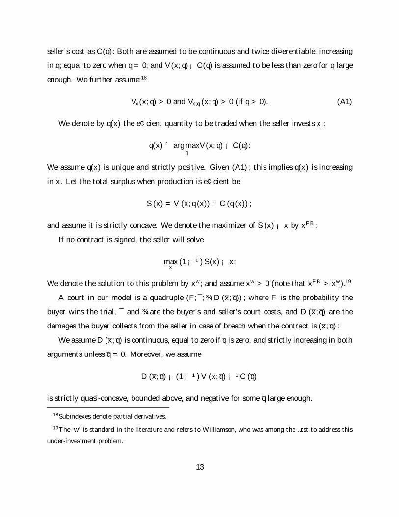
seller’s cost as C(q): Both are assumed to be continuous and twice di¤erentiable, increasing

in q; equal to zero when q = 0; and V (x; q) ¡ C(q) is assumed to be less than zero for q large

enough. We further assume:18

Vx(x; q) > 0 and Vx;q (x; q) > 0 (if q > 0). (A1)

We denote by q(x) the e¢cient quantity to be traded when the seller invests x :

q(x) ´ arg maxq

V (x; q) ¡ C(q):

We assume q(x) is unique and strictly positive. Given (A1) ; this implies q(x) is increasing

in x. Let the total surplus when production is e¢cient be

S (x) = V (x; q (x)) ¡ C (q (x)) ;

and assume it is strictly concave. We denote the maximizer of S (x) ¡ x by xFB:

If no contract is signed, the seller will solve

maxx

(1 ¡ ¹) S(x) ¡ x:

We denote the solution to this problem by xw; and assume xw > 0 (note that xF B > xw).19

A court in our model is a quadruple (F; ¯; ¾; D (x; q)) ; where F is the probability the

buyer wins the trial, ¯ and ¾ are the buyer’s and seller’s court costs, and D (x; q) are the

damages the buyer collects from the seller in case of breach when the contract is (x; q) :

We assume D (x; q) is continuous, equal to zero if q is zero, and strictly increasing in both

arguments unless q = 0. Moreover, we assume

D (x; q) ¡ (1 ¡ ¹) V (x; q) ¡ ¹C (q)

is strictly quasi-concave, bounded above, and negative for some q large enough.

18Subindexes denote partial derivatives.

19The ‘w’ is standard in the literature and refers to Williamson, who was among the …rst to address this

under-investment problem.

13

The canonical example of a damage function is simply D (x; q) = V (x; q), the expectation

damage function.20

Our approach is to take the court (F; ¯; ¾; D (¢)) as given and characterize the optimal

contract for this court and the corresponding equilibrium investment level. We then charac-

terize the set of courts for which contracting is valuable, and the set for which the …rst-best

is achievable.

Two generalizations of this simple court game are discussed in section 6. The …rst one

is to assume there is a set of courts from which parties can choose. The selection of the

court is then included in the original contract. The second generalization is to model the

court game as a rent-seeking game, where the parties optimally choose ¯ and ¾; and their

decisions a¤ect the trial outcome:

Payo¤s

Note that the renegotiation between dates 1 and 2 can take place under two qualitatively

di¤erent scenarios. Given a contract k and an investment level x; it might be optimal for the

buyer not to sue the seller (N) even if no agreement is reached at this renegotiation stage. In

this case, the threat point is determined exclusively by the original contract, and, therefore,

the payo¤ for the buyer after renegotiating would be

¦B;N(k; x) = V (x; q) + ¹ [S (x) ¡ (V (x; q) ¡ C (q))] ;

where V (x; q) is what he would obtain under the original contract (if the parties do not

renegotiate), and the second term is the fraction of the renegotiation surplus the buyer

appropriates.21

20Note that D (x; q) being an approximation to V (x; q) corresponds to the de…nition of expected damages

because we assumed that t is an up-front payment. If we were to assume that t is a payment to be made at

the moment of the transaction, then the expected damages the buyer should be entitled to collect in case of

breach would be only D (x; q) ¡ t (as an approximation to V (x; q) ¡ t): In both cases, the t only serves the

role of dividing the surplus.

In order to implement expectation damages perfectly the court would have to know the buyer’s valuation

function V (x; q) : This might be a strong assumption.

21All payo¤s are net of the up-front payment t:

14

On the other hand, if, given (k; x) ; it is optimal for the buyer to go to court (C) when no

agreement is reached, then the threat point for the renegotiation is given by the payo¤s the

players would obtain if they go to court. Since the parties will settle out of court (S) ; the

payo¤ for the buyer in this case will be what he would obtain if they go to court, ¦B;C(k; x);

plus a fraction ¹ of the renegotiation surplus,22 that is

¦B;S(k; x) = ¹ (¯ + ¾) + ¦B;C(k; x);

where the buyer’s payo¤ from going to court is

¦B;C(k; x) = ¡¯ + F [D (x; q) + ¹S (x)] + (1 ¡ F ) ¦B;N (k; x):

If the buyer wins the trial – with probability F – he collects damages D (x; q) and, since

they are then no longer bound by the original contract, he appropriates a fraction ¹ of the

total surplus. If he loses – with probability 1 ¡ F – he gets what he would have received if

there had been no trial. In both cases, he has to pay his court costs (¯).

Similarly, we can de…ne seller’s payo¤ in the three situations:

¦S;N(k; x) = ¡C (q) + (1 ¡ ¹) [S (x) ¡ V (x; q) + C (q)] ¡ x

¦S;C(k; x) = ¡¾ + F [¡D (x; q) + (1 ¡ ¹) S (x) ¡ x] + (1 ¡ F ) ¦S;N(k; x)

¦S;S(k; x) = (1 ¡ ¹) (¯ + ¾) + ¦S;C(k; x):

Note that we implicitly assume that after they agree on a new contract, the buyer cannot

sue the seller. This is with no loss of generality. One possibility for the players is to agree

on a contract that speci…es only a quantity to be traded and a payment, which leaves the

buyer with no grounds to sue the seller (in our model the buyer sues claiming the seller did

not invest what she committed to investing). Alternatively, the parties can get the payo¤s

speci…ed above by, between 1 and 2, annulling the contract and agreeing on a payment t0;

and later splitting the surplus S (x) according to their bargaining powers. The annulled

contract guarantees the buyer cannot sue.

22By settling out of court the parties are saving the court costs ¯ + ¾: This is the surplus ‘generated’ in

this renegotiation process.

15

4. An Illustrative Example

We present a simple example that illustrates the main point of the paper: even though

investment is not veri…able (the enforcement technology is independent of the investment),

players can use a costly and imperfect court to improve on their implementation problem.

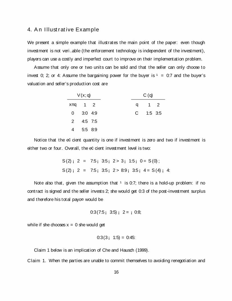
Assume that only one or two units can be sold and that the seller can only choose to

invest 0; 2; or 4: Assume the bargaining power for the buyer is ¹ = 0:7 and the buyer’s

valuation and seller’s production cost are

V (x; q) C (q)

xnq 1 2

0

2

4

3:0 4:9

4:5 7:5

5:5 8:9

q 1 2

C 1:5 3:5

Notice that the e¢cient quantity is one if investment is zero and two if investment is

either two or four. Overall, the e¢cient investment level is two:

S (2) ¡ 2 = 7:5 ¡ 3:5 ¡ 2 > 3 ¡ 1:5 ¡ 0 = S (0) ;

S (2) ¡ 2 = 7:5 ¡ 3:5 ¡ 2 > 8:9 ¡ 3:5 ¡ 4 = S (4) ¡ 4:

Note also that, given the assumption that ¹ is 0:7; there is a hold-up problem: if no

contract is signed and the seller invests 2; she would get 0:3 of the post-investment surplus

and therefore his total payo¤ would be

0:3 (7:5 ¡ 3:5) ¡ 2 = ¡0:8;

while if she chooses x = 0 she would get

0:3 (3 ¡ 1:5) = 0:45:

Claim 1 below is an implication of Che and Hausch (1999).

Claim 1. When the parties are unable to commit themselves to avoiding renegotiation and

16

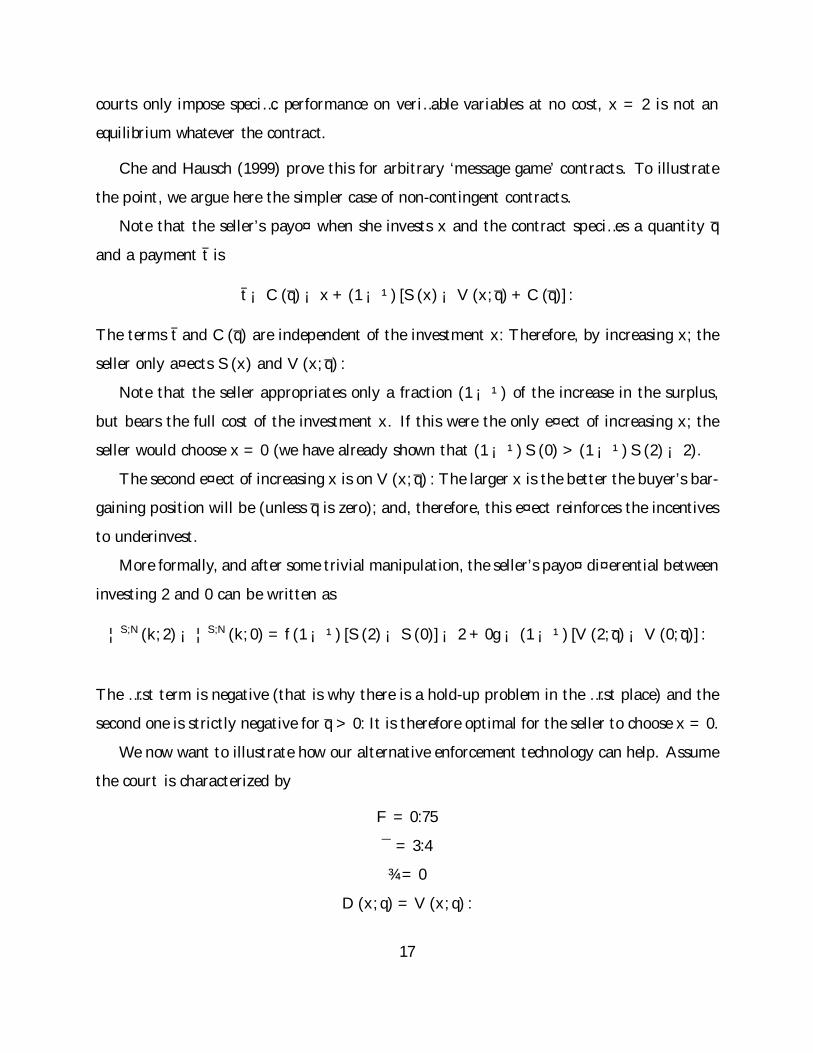
courts only impose speci…c performance on veri…able variables at no cost, x = 2 is not an

equilibrium whatever the contract.

Che and Hausch (1999) prove this for arbitrary ‘message game’ contracts. To illustrate

the point, we argue here the simpler case of non-contingent contracts.

Note that the seller’s payo¤ when she invests x and the contract speci…es a quantity q

and a payment t is

t ¡ C (q) ¡ x + (1 ¡ ¹) [S (x) ¡ V (x; q) + C (q)] :

The terms t and C (q) are independent of the investment x: Therefore, by increasing x; the

seller only a¤ects S (x) and V (x; q) :

Note that the seller appropriates only a fraction (1 ¡ ¹) of the increase in the surplus,

but bears the full cost of the investment x. If this were the only e¤ect of increasing x; the

seller would choose x = 0 (we have already shown that (1 ¡ ¹) S (0) > (1 ¡ ¹) S (2) ¡ 2).

The second e¤ect of increasing x is on V (x; q) : The larger x is the better the buyer’s bar-

gaining position will be (unless q is zero); and, therefore, this e¤ect reinforces the incentives

to underinvest.

More formally, and after some trivial manipulation, the seller’s payo¤ di¤erential between

investing 2 and 0 can be written as

¦S;N(k; 2) ¡ ¦S;N (k; 0) = f(1 ¡ ¹) [S (2) ¡ S (0)] ¡ 2 + 0g ¡ (1 ¡ ¹) [V (2; q) ¡ V (0; q)] :

The …rst term is negative (that is why there is a hold-up problem in the …rst place) and the

second one is strictly negative for q > 0: It is therefore optimal for the seller to choose x = 0.

We now want to illustrate how our alternative enforcement technology can help. Assume

the court is characterized by

F = 0:75

¯ = 3:4

¾ = 0

D (x; q) = V (x; q) :

17

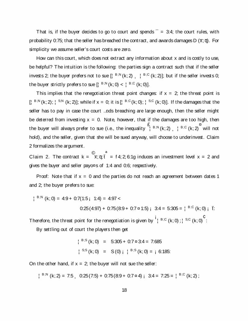
That is, if the buyer decides to go to court and spends ¯ = 3:4; the court rules, with

probability 0:75; that the seller has breached the contract, and awards damages D (x; q). For

simplicity we assume seller’s court costs are zero.

How can this court, which does not extract any information about x and is costly to use,

be helpful? The intuition is the following: the parties sign a contract such that if the seller

invests 2; the buyer prefers not to sue [¦B;N(k; 2) ¸ ¦B;C (k; 2)]; but if the seller invests 0;

the buyer strictly prefers to sue [¦B;N(k; 0) < ¦B;C (k; 0)].

This implies that the renegotiation threat point changes: if x = 2; the threat point is

[¦B;N (k; 2); ¦S;N (k; 2)]; while if x = 0; it is [¦B;C(k; 0); ¦S;C (k; 0)]. If the damages that the

seller has to pay in case the court …nds breaching are large enough, then the seller might

be deterred from investing x = 0. Note, however, that if the damages are too high, then

the buyer will always prefer to sue (i.e., the inequality£¦B;N (k; 2) ¸ ¦B;C (k; 2)

¤will not

hold), and the seller, given that she will be sued anyway, will choose to underinvest. Claim

2 formalizes the argument.

Claim 2. The contract k =©

x; q; tª

= f4; 2; 6:1g induces an investment level x = 2 and

gives the buyer and seller payo¤s of 1:4 and 0:6; respectively.

Proof: Note that if x = 0 and the parties do not reach an agreement between dates 1

and 2; the buyer prefers to sue:

¦B;N (k; 0) = 4:9 + 0:7(1:5 ¡ 1:4) = 4:97 <

0:25 (4:97) + 0:75 (8:9 + 0:7 ¤ 1:5) ¡ 3:4 = 5:305 = ¦B;C (k; 0) ¡ t:

Therefore, the threat point for the renegotiation is given by¡¦B;C (k; 0) ; ¦S;C (k; 0)

¢:

By settling out of court the players then get

¦B;S (k; 0) = 5:305 + 0:7 ¤ 3:4 = 7:685

¦S;S (k; 0) = S (0) ¡ ¦B;S (k; 0) = ¡6:185:

On the other hand, if x = 2; the buyer will not sue the seller:

¦B;N (k; 2) = 7:5 ¸ 0:25 (7:5) + 0:75 (8:9 + 0:7 ¤ 4) ¡ 3:4 = 7:25 = ¦B;C (k; 2) ;

18

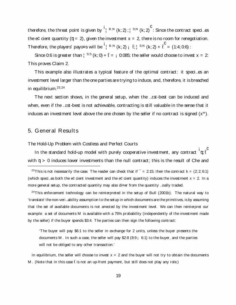
therefore, the threat point is given by¡¦B;N (k; 2) ; ¦S;N (k; 2)

¢: Since the contract speci…es

the e¢cient quantity (q = 2), given the investment x = 2, there is no room for renegotiation.

Therefore, the players’ payo¤s will be¡¦B;N (k; 2) ¡ t; ¦S;N (k; 2) + t

¢= (1:4; 0:6) :

Since 0:6 is greater than ¦S;S (k; 0) + t = ¡0:085; the seller would choose to invest x = 2:

This proves Claim 2.

This example also illustrates a typical feature of the optimal contract: it speci…es an

investment level larger than the one parties are trying to induce, and, therefore, it is breached

in equilibrium.23 ;24

The next section shows, in the general setup, when the …rst-best can be induced and

when, even if the …rst-best is not achievable, contracting is still valuable in the sense that it

induces an investment level above the one chosen by the seller if no contract is signed (xw).

5. General Results

The Hold-Up Problem with Costless and Perfect Courts

In the standard hold-up model with purely cooperative investment, any contract¡q; t

¢with q > 0 induces lower investments than the null contract; this is the result of Che and

23This is not necessarily the case. The reader can check that if ¯ = 2:15; then the contract k = (2; 2; 6:1)

(which speci…es both the e¢cient investment and the e¢cient quantity) induces the investment x = 2. In a

more general setup, the contracted quantity may also di¤er from the quantity …nally traded.

24This enforcement technology can be reinterpreted in the setup of Bull (2001b). The natural way to

‘translate’ the non-veri…ability assumption to the setup in which documents are the primitives, is by assuming

that the set of available documents is not a¤ected by the investment level. We can then reinterpret our

example: a set of documents M is available with a 75% probability (independently of the investment made

by the seller) if the buyer spends $3:4. The parties can then sign the following contract:

‘The buyer will pay $6:1 to the seller in exchange for 2 units, unless the buyer presents the

documents M . In such a case, the seller will pay $2:8 (8:9 ¡ 6:1) to the buyer, and the parties

will not be obliged to any other transaction.’

In equilibrium, the seller will choose to invest x = 2 and the buyer will not try to obtain the documents

M . (Note that in this case t is not an up-front payment, but still does not play any role.)

19

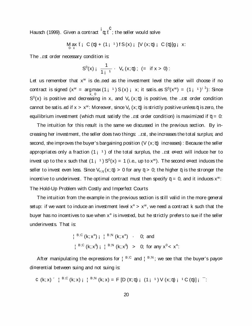
Hausch (1999). Given a contract¡q; t

¢; the seller would solve

Max0·x

t ¡ C (q) + (1 ¡ ¹) fS (x) ¡ [V (x; q) ¡ C (q)]g ¡ x:

The …rst order necessary condition is:

S 0 (x) ¡ 1

1 ¡ ¹· Vx (x; q) ; (= if x > 0) :

Let us remember that xw is de…ned as the investment level the seller will choose if no

contract is signed (xw = arg maxx¸0

(1 ¡ ¹) S (x) ¡ x; it satis…es S 0 (xw) = (1 ¡ ¹)¡1): Since

S 0 (x) is positive and decreasing in x, and Vx (x; q) is positive, the …rst order condition

cannot be satis…ed if x > xw: Moreover, since Vx (x; q) is strictly positive unless q is zero, the

equilibrium investment (which must satisfy the …rst order condition) is maximized if q = 0:

The intuition for this result is the same we discussed in the previous section. By in-

creasing her investment, the seller does two things: …rst, she increases the total surplus; and

second, she improves the buyer’s bargaining position (V (x; q) increases) : Because the seller

appropriates only a fraction (1 ¡ ¹) of the total surplus, the …rst e¤ect will induce her to

invest up to the x such that (1 ¡ ¹) S0 (x) = 1 (i.e., up to xw). The second e¤ect induces the

seller to invest even less. Since Vx;q (x; q) > 0 for any q > 0; the higher q is the stronger the

incentive to underinvest. The optimal contract must then specify q = 0, and it induces xw:

The Hold-Up Problem with Costly and Imperfect Courts

The intuition from the example in the previous section is still valid in the more general

setup: if we want to induce an investment level x¤ > xw, we need a contract k such that the

buyer has no incentives to sue when x¤ is invested, but he strictly prefers to sue if the seller

underinvests. That is:

¦B;C (k; x¤) ¡ ¦B;N (k; x¤) · 0; and

¦B;C (k; x0) ¡ ¦B;N (k; x0) > 0; for any x0 < x¤:

After manipulating the expressions for ¦B;C and ¦B;N ; we see that the buyer’s payo¤

di¤erential between suing and not suing is:

¢ (k; x) ´ ¦B;C (k; x) ¡ ¦B;N (k; x) = F [D (x; q) ¡ (1 ¡ ¹) V (x; q) ¡ ¹C (q)] ¡ ¯:

20

This expression is strictly decreasing in x when q > 0: Therefore, the above two conditions

reduce to ¢ (k; x¤) = 0: Lemma 1 shows that this is a necessary condition to induce the

desired investment level x¤:

Lemma 1. For all x¤ > 0; if x¤ > xw and ¢ (k; x¤) 6= 0; then x¤ is not an equilibrium

investment level of the game de…ned by contract k.

Proof: see Appendix A.

The intuition for this result is simple: if ¢ (k; x¤) > 0 and the seller invests x = x¤;

the buyer will choose to go to court. Given that she will be sued, it is easy to show that

the optimal investment for the seller is some x smaller than xw: On the other hand, if

¢ (k; x¤) < 0; there will exist an investment x¤0 2 [xw; x¤) such that she will not be sued

(¢ (k; x¤0) · 0) and her payo¤ will be larger (¦S;N (k; x¤0) ¸ ¦S;N (k; x¤)).

Note that the necessary condition ¢ (k; x¤) = 0 cannot be satis…ed if ¯ is too large or if

F is too small. Intuitively, in such cases it will never be optimal for the buyer to sue the

seller and, therefore, the seller would have the same incentives as if there were not a costly

court game.25

Let X¤ = fx¤:9k s.t. ¢ (k; x¤) = 0g : Note that if

maxx;q

F [D (x; q) ¡ (1 ¡ ¹) V (x¤; q) ¡ ¹C (q)] ¡ ¯ > 0;

there will be a continuum of contracts such that ¢ (k; x¤) = 0:26

¢ (k; x¤) = 0 is not only necessary for x¤ to be induced, but it also implies that the seller

would not ‘slightly’ underinvest: if she chooses to invest x¤ ¡ "; then it will be optimal for

the buyer to sue and the threat point for the renegotiation will be¡¦B;C ; ¦S;C

¢rather than¡

¦B;N ; ¦S;N¢. For " small, the total surplus will only be slightly a¤ected and ¦B;C (k; x¤ ¡ ")

will be nearly the same as ¦B;N (k; x¤).27 Since the total court expenditures (¯ + ¾) are

25This would also be the case if D (x; q) is too small relative to V (x; q) and C (q) :

26Let us remember the assumptions that all functions are continuous, that V (x; 0) = C (q) = 0; and that

the expression [D (x; q) ¡ (1 ¡ ¹) V (x; q) ¡ ¹C (q)] is negative for q large enough.

27Recall that ¢ (k; x¤) = 0 , ¦B;N (k; x¤) = ¦B;C (k; x¤).

21

positive and non-negligible and the buyer’s payo¤ is ¦B;C (k; x¤ ¡ ") + ¹ (¯ + ¾) ; then it

necessarily holds that the seller’s payo¤ – equal to the total surplus minus the buyer’s payo¤

– is discretely reduced when she invests x¤ ¡ " instead of x¤:

To make sure that the seller does not prefer to ‘severely’ underinvest, we need to compare

her payo¤ when she invests x¤ and will not be sued with her payo¤ if she underinvests and

the parties settle before trial. The proof of Proposition 1 is straightforward.

Proposition 1. An investment level x¤ > xw is induced with a contract k if and only if

¦S;N (k; x¤) ¡ max0·x0

¦S;S (k; x0) ¸ 0; and (*)

¢ (k; x¤) = 0:


Although correct, Proposition 1 is not very informative. It says nothing about the optimal

contract or when condition (*) holds.

In the case the …rst-best level of investment is achievable, there would typically be a

continuum of contracts that can induce it; and all we can say in that case is that the

contract k chosen will satisfy (*) for xFB and ¢¡k; xFB

¢= 0.

However, if the …rst-best is not achievable, then it has to be either because (*) is binding

for the equilibrium x¤, or because for any " > 0 x¤ + " =2 X¤ (i.e., there is no contract k

satisfying ¢ (k; x¤ + ") = 0).28

We need to further explore the restrictions imposed by ¢¡k; xFB

¢= 0 and (*) to be able

to say something about the optimal contract when xFB is not achievable and to characterize

under which circumstances this contract improves over the no contract case.

Lemma 1 implies that, if we want to induce x¤ 2 X¤; we can restrict attention to contracts

satisfying ¢ (k; x¤) = 0: When this condition is satis…ed, equation (*) can be written as

¹ (¯ + ¾) + (1 ¡ ¹) [S (x¤) ¡ S (xc)] ¡ x¤ + xc ¡ (1 ¡ F ) (1 ¡ ¹) [V (x¤; q) ¡ V (xc; q)] ¸ 0;

(*’)

28As will become apparent, if an investment x > xw cannot be induced in equilibrium, then no other x0 > x

will be inducible. Moreover, if x can be induced in equilibrium, then any x00 2 [xw; x] will be inducible.

22

where xc solves seller’s ‘cheating’ problem: max0·x

¦S;S (k; x) : The above expression is decreas-

ing in q since x¤ > xw ¸ xc (in the proof of Lemma 1 we show that xw ¸ xc).29 There-

fore, we can restrict attention to the contract with the lowest possible q that also satis…es

¢ (k; x¤) = 0: If such a contract does not satisfy (*’); then x¤ cannot be induced.

For all x¤ 2 X¤; de…ne

bbq (x; x¤) ´ min fq : F [D (x; q) ¡ (1 ¡ ¹) V (x¤; q) ¡ ¹C (q)] ¡ ¯ = 0g :

Recall that we assumed that D (x; q) is increasing in x; then it is straightforward to show

that bbq (x; x¤) is decreasing in x and increasing in x¤ and, therefore, we can restrict attention

to contracts where x = X: Let bq (x¤) ´ bbq (X; x¤) :

Proposition 2. Let xM be the maximum investment level that can be induced by any

contract: If xM > xw and F < 1; the unique contract that induces xM is (x; q) =¡X; bq ¡

xM¢¢

:


Corollary 1. If an investment level x¤ > xw can be induced with a contract (x; q) ; then it

can also be induced with the contract (X; bq (x¤)) :


Knowing what the optimal contract looks like (Proposition 2) and what conditions are

necessary and su¢cient to induce a particular investment level (Proposition 1), it is im-

mediate to characterize for which courts contracting will be valuable (an x¤ > xw can be

induced), and when the …rst-best will be achievable. This is done in Propositions 3 and 4

and illustrated with a numerical example below.

29The problem max0·x0

¦S;S (k; x0) can be rewritten as

max0·x0

K + (1 ¡ ¹) S (x0) ¡ x0 ¡ (1 ¡ F ) (1 ¡ ¹) V (x0; q) ;

where K is a constant. The terms including x0 in the above expression are the same (with opposite sign)

that we have in (*’); therefore, by the envelope theorem, we can restrict attention to the direct e¤ect of q

on (*’).

23

We derive our results in terms of the court game parameters (F; ¯; ¾) and the damage

function D (x; q) : Abusing notation, we denote by xc (q; F ) the optimal ‘cheating’ investment:

xc (q; F ) ´ arg max0·x

¦S;S (k; x) ;

and by bq (x; ¯=F ) the smallest q that satis…es

F [D (X; q) ¡ (1 ¡ ¹) V (x; q) ¡ ¹C (q)] ¡ ¯ = 0:

Proposition 3. Contracting has value, i.e. an investment x¤ > xw can be induced, if and

only if

maxq

F [D (X; q) ¡ (1 ¡ ¹) V (xw; q) ¡ ¹C (q)] ¡ ¯ > 0; and

¹ (¯ + ¾) + G (xw; F; ¯) > 0;

where

G (x; F; ¯) ´ (1 ¡ ¹) [S (x) ¡ S (xc (bq (x; ¯=F ) ; F ))] ¡ x + xc (bq (x; ¯=F ) ; F ) ¡(1 ¡ ¹) (1 ¡ F ) [V (x; bq (x; ¯=F )) ¡ V (xc (bq (x; ¯=F ) ; F ) ; bq (x; ¯=F ))] :


The …rst inequality is required for the existence of a contract k satisfying ¢ (k; x¤) = 0 for

some x¤ > xw; and the second inequality implies that the contract (X; bq (xw; ¯=F )) satis…es

(*’) for xw as a strict inequality. Then, by continuity, there must be a contract that induces

an investment level above x¤ > xw:

Proposition 4. The …rst-best level of investment can be induced if and only if

maxq

F£D (X; q) ¡ (1 ¡ ¹) V

¡xFB; q

¢ ¡ ¹C (q)¤ ¡ ¯ ¸ 0; and

¹ (¯ + ¾) + G¡xF B; F; ¯

¢ ¸ 0:


The proof is similar to the one of Proposition 3. It relies on the fact that an optimal

contract is¡X; bq ¡

xF B; ¯=F¢¢

:

24

Example to Illustrate Propositions 3 and 4

Assume:

V (x; q) = D (x; q) = 4q¡1 + x1=4

¢C (q) = 4q + 2q2

¹ = 0:5

¾ = 0:25

It is easy to show that for this example xFB = 1 and xw = 0:25:

Given a value of ¯ and an investment level x¤ 2 [0; X] that we want to induce, we de…ne

Fm (¯; x¤) as the smallest F 2 [0; 1] that satis…es

maxq

F [D (X; q) ¡ (1 ¡ ¹) V (x¤; q) ¡ ¹C (q)] ¡ ¯ ¸ 0; and

¹ (¯ + ¾) + G (x¤; F; ¯) ¸ 0:

Note that the above expressions are both increasing in F: Then, if the buyer’s probability of

winning in court (F ) is larger than Fm (¯; x¤), there will exist a contract k that induces an

investment x¤ (i.e., there will exist k such that ¢ (k; x¤) is zero and (*’) is satis…ed). If for

a particular pair (¯; x¤) there is no F 2 [0; 1] that satis…es both conditions, then x¤ cannot

be induced.

Figure B.1 illustrates this discussion for the numerical example proposed above. Figure

B.2 shows how Fm is a¤ected when ¾ increases to 0:35.

The case of F = 1

Two de…nitions are needed to characterize what can be implemented for the particular

case of F = 1: Let x (®) be the x ¸ xw that satis…es

(1 ¡ ¹) [S (xw) ¡ S (x)] ¡ xw + x = ® (see Figure B.3);

and let ex be the largest x for which there is a contract that satis…es ¢ (k; ex) = 0; that is:

ex ´

8><>:X if max

qD (X; q) ¡ (1 ¡ ¹) V (X; q) ¡ ¹C (q) ¡ ¯ ¸ 0;

x : maxq

D (X; q) ¡ (1 ¡ ¹) V (x; q) ¡ ¹C (q) ¡ ¯ = 0 otherwise:

25

Corollary 2. Assume ex ¸ xw: If F = 1; any x 2 [xw; min fex; x (¹ (¯; ¾))g] can be induced.


The proof of Corollary 2 uses the fact that when F = 1 the optimal ‘cheating’ investment

level is xc = xw and condition (*’) simpli…es to ¹ (¯ + ¾) + (1 ¡ ¹) [S (x¤) ¡ S (xw)] ¡ x¤ +

xw+ ¸ 0: The de…nition of x (¹ (¯ + ¾)) implies that the previous expression is non-negative

for any x¤ 2 [xw; x (¹ (¯ + ¾))] :

Comparative Statics

The following corollaries are derived from Propositions 1 and 2.

Corollary 3. Assume the maximum inducible investment level xM is smaller than X: If ¾

increases, then xM strictly increases unless

maxq

F£D (X; q) ¡ (1 ¡ ¹) V

¡xM ; q

¢ ¡ ¹C (q)¤ ¡ ¯ = 0:


Intuitively, if maxq

F£D (X; q) ¡ (1 ¡ ¹) V

¡xM ; q

¢ ¡ ¹C (q)¤¡¯ > 0 and xM is the maxi-

mum investment level that can be induced, then it has to be that (*’) is binding. An increase

in ¾ eases this constraint.

Corollary 4. Assume the maximum inducible investment level xM is smaller than X: If F

increases, then xM strictly increases:


A larger F eases (*’) and increases maxq

F£D (X; q) ¡ (1 ¡ ¹) V

¡xM ; q

¢ ¡ ¹C (q)¤ ¡ ¯;

which allows us to …nd a contract k0 such that ¢ (k0; x0) = 0 for some x0 > xM and (*’) is

still satis…ed.

Corollary 5. If maxq

F£D (X; q) ¡ (1 ¡ ¹) V

¡xM ; q

¢ ¡ ¹C (q)¤ ¡ ¯ = 0 and ¯ is increased,

then xM strictly decreases.

26

The proof is straightforward: q being the maximizer of the left hand side of the above

expression implies that if ¯ increases then the only way the equality can be satis…ed is by

decreasing xM :

The e¤ect of ¯ on xM is not always negative. If maxq

F£D (X; q) ¡ (1 ¡ ¹) V

¡xM ; q

¢ ¡ ¹C (q)¤¡

¯ > 0 we cannot tell which is the e¤ect of ¯ on xM : In that case (and since xM is the largest

x we can induce), it necessarily holds that the inequality (*’) is binding:

¹ (¯ + ¾) + G (x; F; ¯) = 0:

Then, an increase in ¯ has two e¤ects that go in opposite directions: the …rst term above

obviously increases, but the increase in ¯ also a¤ects G (x; F; ¯) negatively.

Recall the de…nition, G¡xM ; F; ¯

¢is

(1 ¡ ¹)£S

¡xM

¢ ¡ S¡xc

¡bq ¡xM ; ¯=F

¢; F

¢¢¤ ¡ xM + xc¡bq ¡

xM ; ¯=F¢

; F¢ ¡

(1 ¡ ¹) (1 ¡ F )£V

¡xM ; bq ¡

xM ; ¯=F¢¢ ¡ V

¡xc

¡bq ¡xM ; ¯=F

¢; F

¢; bq ¡

xM ; ¯=F¢¢¤

:

When ¯ is increased, the contracted quantity (q = bq (x; ¯=F )) has to increase in order to

satisfy ¢¡k; xM

¢= 0: That increase in q makes the last term above larger in absolute value

(since Vq

¡xM ; q

¢ ¡ Vq (xc; q) > 0), so that G (x; F; ¯) decreases as ¯ increases (assuming

F < 1).30

6. Extensions of the Basic Model - Discussion

Endogenous Court Expenditure

We have characterized above for which ‘courts of law’ – parameters (F; ¯; ¾) and function

D (x; q) – contracting has value and when the …rst-best can be achieved. We have chosen

such a simple model only for expositional ease and to highlight the main result: a costly

court, unable to obtain any information about the facts of the case, can help the parties.

30Consider Figure B.1 and assume xM = 1 and F = 0:5: Then if ¯ is small (approximately 0:4) an increase

in ¯ would increase xM ; while if ¯ is large (approximately 0:9) then its increase would decrease xM :

27

There are at least two ways in which the model can be enriched and the results not be

a¤ected (or strengthened). First, we could endogenize ¯ and ¾ by assuming the parties’

expenditures a¤ect their probability of winning the trial and the amount of damages to be

paid. To remain consistent with the assumption that investment is not veri…able, neither

the probability of winning nor the damages should depend directly on the investment made.

Indirectly, the investment made by the seller will a¤ect the buyer’s incentives to go to court

(as in the simplest model) and to spend money on the litigation process.

In this more general model, we would have F (¢) and D (¢) as functions of ¯ and ¾, and

the parties would choose them to maximize their expected payo¤s. The court game would

then look like a rent-seeking game with an endogenous prize. Under suitable assumptions,

we can show that the equilibrium of this court game, (¯¤; ¾¤), is unique and strictly positive.

The outcome of this game, i.e. ¯¤; ¾¤; F (¯¤; ¾¤) ; and D (k; ¯¤; ¾¤), is what we considered

here as our primitive ‘court of law.’

This way of extending the court game is appealing. The quality of lawyers (and their

salaries), the time spent to prepare for trial, the expert witnesses hired, etc. all a¤ect the

probability of winning or losing, and the amount of damages.31

Optimal Choice of Courts

Another extension (that could be combined with the previous one) is to assume that

parties have some discretion over which court to choose. In the simpler setup, we could

assume there is a set of available courts from which the parties can choose and they will pick

the one that allows them to induce the most e¢cient outcome possible. A way of considering

31An example that comes immediately to mind is the criminal case against O.J. Simpson. Despite the

enormous physical evidence, the defendant, after hiring a ‘dream team’ of lawyers and spending something

between 4 and 7 million dollars (Source: CNN) was found not guilty.

This is true not only in criminal cases, quoting S. Macaulay (1985), “if lawyers of equal ability represent

clients with equal resources and willingness to invest them in a case falling under Article II [of the Uniform

Commercial Code], the case will end in a tie. Those who can a¤ord to play invest in the skills of large law

…rms. They play the litigation game by expanding procedural complexity to draw out the process. Others

who cannot a¤ord to invest as much must drop out.”

28

this alternative together with the previous one is by assuming that F and D (x; q) depend

not only on what the parties spend in court, but also on the contract the parties sign.

This extension is consistent with what we observe in reality. Parties can choose, to

some extent, the particular court they want to solve their potential disputes, and they do so

strategically. According to the Uniform Commercial Code (§1-105(1)), “...when a transaction

bears a reasonable relation to this state and also to another state or nation the parties may

agree that the law either of this state or of such other state or nation shall govern the rights

and duties.”32

The particular court chosen will a¤ect the litigation costs of the parties. If two corpo-

rations are located in two di¤erent states and they choose to be governed by the state law

of one of the parties’ state, we should expect the other one to face higher litigation costs

derived from having to hire lawyers licensed in the other state. If parties choose the law of

a third state,33 then both parties would probably face higher litigation costs.

The election of the particular state court may also a¤ect the probability of one or the

other party winning and the potential damages. Some state courts are more experienced than

others in particular matters and therefore their ruling may be easier to predict. Juries in

some states may be biased against large corporations and be prone to award large damages.

Choosing a particular court is not limited to the election of the state law that shall

govern the relationship. Even for the same state law, parties can still a¤ect their expected

litigation costs when designing the contract. For example, parties can agree on the contract

that any disputes will be solved by arbitration, which is typically cheaper than going to

trial.34 Moreover, once parties agree in the contract they will solve any disputes through

arbitration, they can still include di¤erent clauses that will a¤ect the cost of the arbitration

32If the two parties do not stipulate which state’s law they want to govern their contract, then, should

a dispute develop, each state will have a set of default rules called ‘choice of law rules.’ The default rules

typically say that the state that has the ‘greatest interest in the case’ should rule on the dispute.

33They can do so only if the transaction is somehow related to this third state.

34Arbitration is one of the several Alternative Dispute Resolution (A.D.R.) methods parties can choose.

Others are mediation, early neutral evaluation, and conciliation.

29

mechanism.35

Hybrid Investment

Although we developed the case of purely cooperative investment, the main results extend

to the case of hybrid investment (investment a¤ects both the buyer’s value and the seller’s

costs), provided it is not ‘too sel…sh’.

In the case of cooperative investment our mechanism works because, given a contract

that satis…es ¢ (k; x¤) = 0; if the seller underinvests, the buyer has an incentive to go to

court. The intuition behind this is simple: the lower the investment, the lower the value of

the q units the buyer is committed to buy. Below a critical value of x (that depends on q)

the buyer simply prefers to go to court and, with probability F , avoid the commitment to

buy those q units.

In the case of hybrid investment, this intuition is incomplete. If the seller decreases her

investment, it will also a¤ect her costs. If her costs increase as she decreases x,36 her threat

point for the renegotiation worsens and this favors the buyer, who appropriates a fraction ¹

of the renegotiation surplus.

Analytically, the buyer’s payo¤ di¤erential between going to court or not is given by

¢ (k; x) = F [D (x; q) ¡ (1 ¡ ¹) V (x; q) ¡ ¹C (x; q)] ¡ ¯:

In the case of cooperative investment, ¢ (k; x) = 0 guarantees ¢ (k; x0) > 0 for any x0 < x:

But in the case of hybrid investment, ¢ (k; x) will be increasing or decreasing in x depend-

35Quoting DiCarlo (2002), ”they [arbitration clauses] can limit or eliminate the depositions, interrogatories,

document requests, and pretrial motions that are responsible for much of the sometimes crushing expense

of litigation. In recent years, courts have allowed the contracting parties broad discretion to make up any

rules they wish concerning who will hear the dispute and what rules will govern the outcome.”

36So far we assumed x is a quality enhancing investment and, therefore, it increases the buyer’s valuation

for the good.

In the case the investment a¤ects both the quality of the good and the production costs, there is no

‘natural’ assumption about the e¤ect of x on the production costs. For example, a higher x could be a better

quality and more expensive painting for cars that requires a di¤erent painting process. This high quality

painting process could, in principle, be cheaper or more expensive than the low quality one.

30

ing on the sign of ¡ (1 ¡ ¹) Vx (x; q) ¡ ¹Cx (x; q) : Then, our results would extend, mutatis

mutandis, to the case of hybrid investment as long as (1 ¡ ¹) Vx (x; q) > ¡¹Cx (x; q) :

Purely Sel…sh Investment

Consider now the case when seller’s investment a¤ects only her own costs and assume

Cx (x; q) < 0 and Cxq (x; q) < 0. In this case, Edlin and Reichelstein (1996) show that the

…rst-best can be achieved with a non-contingent contract. This result is derived for two

di¤erent court remedies, expected damages and speci…c performance. As is standard in the

literature, the breaching refers to one of the parties refusing to complete the transaction

and it is assumed that the court, at no cost, either enforces the contract (imposes speci…c

performance) or awards damages at no cost for the parties.

We reconsider the result in our setup assuming, as we have so far, that the buyer can

claim that the seller is not ful…lling other terms of the contract, di¤erent from the delivery

of the goods (as in most of the literature, we are assuming the delivery/acceptance of the

goods can be enforced at no cost).

The incentives for the buyer to sue are driven, as in the cooperative investment case, by

the payo¤ di¤erential between suing and not suing. In the case of sel…sh investment, and

assuming D (q) = V (q) ; this di¤erential can be written as

¢ (q; x) = F¹ [V (q) ¡ C (x; q)] ¡ ¯;

the buyer would sue i¤ ¢ (q; x) > 0:37

Logically, if ¢¡q; xF B

¢ · 0 for any q; then the buyer will never sue the seller and the

e¢ciency result of Edlin and Reichelstein (1996) will hold in our setup. Assume, for the

contrary, that ¢¡q; xFB

¢> 0 for some q; and de…ne

qL

¡xFB

¢ ´ min©

q : ¢¡q; xF B

¢= 0

ªqH

¡xFB

¢ ´ max©

q : ¢¡q; xF B

¢= 0

ª37Note that since the investment is sel…sh it does not a¤ect the buyer’s valuation. Then, the only relevant

variable for the contract is q:

31

Proposition 5 below identi…es under which conditions the …rst-best is not achievable. For

simplicity we maintain the assumption that D (q) = V (q).38

Proposition 5. The …rst-best cannot be achieved if

qL

¡xFB

¢< q

¡xFB

¢< qH

¡xF B

¢; and (+)

Cx

¡xFB; qH

¡xF B

¢¢> ¡ 1

1 ¡ F: (++)


The intuition for this result is as follows. An investment level x¤ can, in principle, be

induced with two di¤erent types of contracts: one in which the buyer has no incentives to

sue (¢ (k; x¤) · 0) ; and one in which the buyer would optimally sue (¢ (k; x¤) > 0) :

If we want to induce xFB with a contract of the …rst type, then q = q¡xFB

¢is required

(see Appendix A). However, if q¡xFB

¢ 2 (qL (x) ; qH (x)) ; it will be optimal for the buyer to

sue if q = q¡xF B

¢and, therefore, there is no contract of the …rst type that induces xFB:

We show in Appendix A that if we want to induce xF B with the second type of contracts,

then q has to satisfy Cx

¡xFB; q

¢= ¡ 1

1¡F(note that for any F > 0 such a q will be greater

than q¡xFB

¢). However, if Cx

¡xFB; qH

¡xFB

¢¢> ¡ 1

1¡F; then the required q will be too

large and the buyer will have no incentives to sue. Therefore xFB cannot be induced with

the second type of contract.

Note that the converse of Proposition 5 is not true. If (+) does not hold, then a contract

specifying q = q¡xFB

¢will induce x = xF B: However, if (+) still holds but (++) does not,

then x = xFB is not guaranteed. It could be the case that the seller, facing a contract that

speci…es q such that Cx

¡xF B; q

¢= ¡ 1

1¡F; …nds it optimal to choose an investment x0 < xFB

such that the buyer will not sue her. q satisfying Cx

¡xFB; q

¢= ¡ 1

1¡Fonly guarantees that

the seller will not deviate to an x0 such that the buyer still …nds it optimal to sue.

It is important to highlight that the negative result of Proposition 5 does not hold if

there is uncertainty either about the buyer’s valuation or the seller’s costs. Suppose the

38We maintain our assumptions about D (x; q) ¡ (1 ¡ ¹) V (x; q) ¡ ¹C (q) made in Section 3. For the case

of sel…sh investment and assuming D (q) = V (q) ;.the assumptions are simply that V (q)¡C (x; q) is strictly

quasi-concave and negative for q large enough.

32

uncertainty is captured by the variable ¸ that is continuously distributed on its support£¸; ¸

¤: The payo¤ di¤erential between going and not going to court for the buyer will now

depend also on ¸; so we can de…ne

q00H

¡xF B

¢ ´ min©

q : q0 > q ) ¢¡q0; xF B; ¸

¢ · 0; 8 (q; ¸)ª

:

Now, if q¡xF B

¢is larger than q00

H

¡xF B

¢; then a contract specifying q = q

¡xF B

¢will give

the buyer no incentives to sue (for any ¸) if x = xFB; and x = xFB will be the solution to

the seller’s problem given that she will not be sued.

Suppose then that q¡xFB

¢is smaller than q00

H

¡xF B

¢and let Q > q00

H

¡xF B

¢be such that

V (Q; ¸) ¡ C (X; Q; ¸) · 0 8¸ 2 £¸; ¸

¤: Then, if a contract speci…es q = Q; the buyer will

not sue the seller (for any x). It is trivial to show that the seller will choose an investment

level x > xF B:

On the other hand, if the contract speci…es a very small q (i.e., q = 0), the seller will

choose some x0 < xFB: Since the seller’s payo¤ varies continuously with q; by the intermediate

value theorem there has to be a q 2 (0; Q) such that the seller invests xFB:

Liquidated Damages - Voided Contracts

Similar results to those obtained in Section 5 can be derived if we assume courts would

enforce any level of liquidated damages or if we assume that the court, rather than awarding

damages to compensate the buyer, would simply void the contract with probability F .

The case of liquidated damages is straightforward. Let L be the level of damages stipu-

lated in a contract k0,39 the payo¤ di¤erential for the buyer between suing and not suing is

now:

¢ (k0; x) = F [L ¡ (1 ¡ ¹) V (x; q) ¡ ¹C (q)] ¡ ¯:

To induce some x¤ > xw we still have to restrict attention to contracts satisfying

¢ (k0; x) = 0: The only di¤erence with the case of expected damages is that now a large

39The parties will include an investment level in the contract only if it is necessary to give the buyer

grounds for suing. For the analysis made, the relevant contract will just be (L; q) : Again, t only determines

the division of the surplus.

33

¯ is not necessarily a problem. In the case of expected damages and for ¯ ‘too large’, it

might be that maxk

¢ (k; x¤) < 0 and, therefore, x¤ would not be inducible. With liqui-

dated damages, by simply stipulating a larger L; this problem is solved. The only relevant

constraint is then (*’).

The case in which the court voids the contract when it …nds breach is analytically identical

to the case of liquidated damages. If the contract is voided, then the parties will not be

committed to any transaction and the seller will have to return any money paid by the

buyer in advance.

The payo¤ di¤erential for the buyer is

¢ (k00; x) = F£t ¡ (1 ¡ ¹) V (x; q) ¡ ¹C (q)

¤ ¡ ¯:

Note that in this case t plays a non-trivial role; it has to be chosen to satisfy ¢ (k00; x) = 0:40

Therefore, the parties cannot use t to achieve the division of the surplus they desire. They

must rely on a side payment to do this. This payment cannot be part of the contract nor

can it be legally associated to the transaction, or else it would be reversed when the contract

is voided.

7. Conclusions

We have considered a hold-up model with the following characteristics: only one party

invests, her investment is purely cooperative, and the parties can renegotiate the original

contract before going to court and/or after the court rules. The renegotiation process is

exogenously given. The main di¤erence with previous literature is the ‘enforcing technology’.

Unlike most of the literature where courts enforce contracts at no cost, we assume costly

litigation. The non-investing party can sue the other one claiming breach, and has a pos-

itive probability of prevailing in the trial.41 To be consistent with the assumption of non-

veri…ability of the investment, we assume that no information about the investment made is

40The ‘relevant contract’ is, in this case, the pair¡t; q

¢:

41The breaching may refer to the seller underinvesting or not ful…lling some other conditions of the contract.

34

revealed in the litigation process.

In this set up, we …nd that parties can improve over the non-contracting case by signing a

simple contract that can later be renegotiated. The contract is such that if the seller invests

the level the parties are trying to induce, the buyer’s payo¤ is the same whether he chooses

to sue or not. Therefore, for any investment level below the one parties intend to induce the

buyer will …nd optimal to sue the seller.

Although the trial stage is never reached (parties can always renegotiate and avoid paying

the court costs), when the seller underinvests the threat point for the renegotiation changes

and this can be enough to discourage the underinvesting.

To make our point clear we chose a very simple enforcement technology. A more so-

phisticated court model could be developed where the trial outcome would depend on the

players’ expenditure on the court game. Moreover, in reality we can expect the parties being

able to a¤ect, by changing the contract clauses, not only the probability of success in a trial

in favor of one or the other party but also the equilibrium court costs. We discussed these

possibilities in Section 6.

Our results give a plausible explanation of why we do not see in reality complicated

mechanisms as the ones suggested in the literature (i.e., message games or mechanisms to

avoid renegotiation).42 It may be that parties really do not need these mechanisms because

with simple contracts (and courts like the ones we assumed) they may achieve (or at least

approximate) the …rst-best outcome.

It is well known in the mechanism design literature that two parties can improve on their

implementation problem if they are allowed to include a third party in the contract or if they

can commit themselves to burning money. Our game structure is equivalent to a contract

where the buyer, after observing the investment made by the seller, sends a message that

determines, as speci…ed in the contract, a transfer from the buyer to the seller, transfers from

the buyer and seller to the third party (or simply how much money each party has to burn),

42For an interesting discussion about the possibility of parties committing themselves not to renegotiate

see Hart & Moore (1999) and Tirole (1999).

35

and, with some probability, a change in the status quo point for the renegotiation. Before

sending that message, the buyer and seller are allowed to renegotiate the original contract.

By choosing the appropriate message-transfers functions, parties would be able to induce

the …rst-best level of investment.43

It is also well established that this kind of contracts does not help when the third party

can collude with one of the players, or if the parties have no way of committing themselves

to burning money. In our model, we make use of a real institution (the court) that allows

the parties to commit themselves to burning money: for the buyer to be compensated for the

alleged breach, he and the seller have to waste resources in the court game (lawyer fees, etc.).

Courts are particularly appealing as third parties because, ideally, they will not collude with

any of the parties. The burning money process is appealing as long as we consider realistic

the assumptions made about the way courts work.

43In our setup, the …rst-best may or may not be achievable, depending on the particular money burning

and seller-buyer transfer technology. The parties can manipulate this technology to some extent with the

initial contract, but they are restricted by the way the court works.

36

A. Appendix: Proofs Missing from the Text

Proof of Lemma 1.

- Suppose the seller chooses x¤ > xw and ¢ (k; x¤) > 0: Then the buyer will strictly prefer

to sue the seller and, since litigation is costly, they will settle out of court. The seller would

solve

maxx0

¦S;S (k; x0) :

Let xc be the solution to this problem. Then, the …rst order necessary condition requires:

(1 ¡ ¹) Sx (xc) ¡ 1 ¡ (1 ¡ ¹) (1 ¡ F ) Vx (xc; q) · 0; ( = if xc > 0).

Recall x¤ > xw , (1 ¡ ¹) S 0 (x¤) < 1: Therefore the …rst order condition is not satis…ed if

xc = x¤:

- Suppose the seller chooses x¤ > xw and ¢ (k; x¤) < 0: By continuity, there exist " such

that x¤ ¡ " ¸ xw and ¢ (k; x¤ ¡ ") · 0: Then

¦S;N (k; x¤ ¡ ") ¡ ¦S;N (k; x¤) = (1 ¡ ¹) [S (x¤ ¡ ") ¡ S (x¤)] ¡ x¤ + " + x¤ +

(1 ¡ ¹) [V (x¤; q) ¡ V (x¤ ¡ "; q)] > 0

since both lines on the right hand side are greater than zero. Therefore, it is not optimal for

the seller to invest x¤ > xw:

Proof of Proposition 1.

) By assumption, there is k such that

¢ (k; x¤) = 0 and ¦S;N (k; x¤) ¡ max0·x0

¦S;S (k; x0) ¸ 0:

Facing such a contract, the seller has to choose her investment level: if she chooses x0 < x¤;

then the buyer will prefer to sue

¢ (k; x¤) = 0 ) ¢ (k; x0) > 0 if x0 < x¤:

The parties would settle out of court and the seller would end up with ¦S;S (k; x0) ; which,

by assumption, is smaller than what she would get by investing x¤.

37

An argument similar to the one made for the proof of Lemma 1 implies she would never

optimally choose x0 > x¤ ¸ xw when ¢ (k; x¤) = 0:

( (by contradiction)

-Suppose x¤ is induced by contract k but ¢ (k; x¤) 6= 0: Lemma 1 shows this is not possible.

-Suppose that for any contract k such that ¢ (k; x¤) = 0; ¦S;N (k; x¤) ¡ max0·x0

¦S;S (k; x0) < 0

holds. Then obviously the seller prefers to invest the x0 that solves max0·x0

¦S;S (k; x0) ; which is

always smaller than or equal to xw and therefore x¤ > xw is not induced in equilibrium.

Proof of Proposition 2. (by contradiction).

* Suppose (x; q) induces xM and x < X:

By Proposition 1 it must be that

¢¡(x; q) ; xM

¢= 0, and

¦S;N¡(x; q) ; xM

¢ ¡ ¦S;S ((x; q) ; xc (q; F )) ¸ 0:

Consider the contract³

x;bbq ¡x; xM

¢´and notice that

¢³³

x;bbq ¡x; xM

¢´; xM

´= 0;

and since bbq ¡x; xM

¢ · q; F < 1, and Vx;q (x; q) > 0; then

¦S;N³³

x;bbq ¡x; xM

¢´; xM

´¡ ¦S;S

³³x;bbq ¡

x; xM¢´

; xc³bbq ¡

x; xM¢

; F´´

¸ 0:

- In the neighborhood of³

x;bbq ¡x; xM

¢; xM

´, the function ¢ (¢) is strictly increasing in x;

increasing in q, and strictly decreasing in x: Therefore, there exist " > 0; q0 such that

q0 < bbq ¡x; xM

¢and ¢

¡(X; q0) ; xM + "

¢= 0:

- The function ¦S;N¡(x; q) ; xM

¢¡¦S;S ((x; q) ; xc (q; F )) is strictly decreasing in q (for F < 1).

Using the envelope theorem, it is then immediate to conclude that

¦S;N¡(X; q0) ; xM

¢ ¡ ¦S;S ((X; q0) ; xc (q0; F )) > 0:

Then, by continuity, there exist ± 2 (0; ") such that

¦S;N¡(X; q0) ; xM + ±

¢ ¡ ¦S;S ((X; q0) ; xc (q0; F )) ¸ 0:

38

- If ± > "; then xM + " can be induced with the contract (X; q0) :

- If " > ±; then xM + ± can be induced with the contract¡X; bq ¡

xM + ±¢¢

:44

* Suppose (x; q) induces xM ; x = X and q 6= bq ¡xM

¢:

- Since ¢¡k; xM

¢= 0 is necessary for xM to be implemented (Lemma 1), the de…nition ofbq ¡

xM¢

(smallest q such ¢¡(X; q) ; xM

¢= 0) implies that q > bq(xM):

- The assumption of strict quasi-concavity of D (x; q) ¡ (1 ¡ ¹) V¡xM ; q

¢ ¡ ¹C (q) implies

¢¡(X; q0) ; xM

¢> 0 for any q0 2 ¡bq ¡

xM¢

; q¢

:

Therefore, there exists " > 0 and q0 2 ¡bq ¡xM

¢; q

¢such that ¢

¡(X; q0) ; xM + "

¢= 0:

Moreover, for any "0 < " there is q0"0 2 ¡bq ¡

xM¢

; q0¢ such that ¢¡(X; q0

"0) ; xM + "0¢ = 0:

- Since (x; q) induces xM ; Vqx (x; q) > 0; F < 1; and q > bq(xM); then

¦S;N¡¡

X; bq(xM)¢

; xM¢ ¡ ¦S;S

¡¡X; bq(xM)

¢; xc

¡bq(xM); F¢¢

> 0:

- By continuity there is some ± 2 (0; ") such that

¦S;N¡(X; q0

±) ; xM + ±¢ ¡ ¦S;S ((X; q0

±) ; xc (q0±; F )) ¸ 0;

therefore the contract (X; q0±) induces the investment level xM + ± > xM :

Proof of Corollary 1. Immediate from the proof of proposition 2.


(- Suppose max

qF [D (X; q) ¡ (1 ¡ ¹) V (xw; q) ¡ ¹C (q)] ¡ ¯ · 0: Then there is no (x; q)

satisfying ¢ (k; x) = 0 for any x > xw: Lemma 1 implies then that no x > xw can be

induced.

- Suppose ¹ (¯ + ¾) + G (xw; F; ¯) · 0: Note that by Corollary 1 we can restrict attention to

contracts of the form (X; bq (¢)) : Note also that G (x; F; ¯) is decreasing in x : as x increases

44Note that bq ¡xM + ±

¢is well de…ned: ¢

¡(X; q0) ; xM + "

¢= 0 and " > ± imply ¢

¡(X; q0) ; xM + ±

¢>

0: Recall also that ¢¡(X; 0) ; xM + ±

¢< 0: Therefore, by continuity, there is some q00 < q0 such that

¢¡(X; q00) ; xM + ±

¢= 0:

39

bq (x; ¯=F ) increases and G (x; F; ¯) decreases by

(1 ¡ ¹) (1 ¡ F ) [Vq (x; bq (x; ¯=F )) ¡ Vq (xc (bq (x; ¯=F ) ; F ) ; bq (x; ¯=F ))] :

Then ¹ (¯ + ¾) + G (x; F; ¯) < 0 8x > xw; and, by Proposition 1, no x > xw can therefore

be implemented.

)- By Corollary 1 we can restrict attention to contracts of the form (X; bq (¢)) : By continuity,

if ¹ (¯ + ¾) + G (xw; F; ¯) > 0 and maxq

F [D (X; q) ¡ (1 ¡ ¹) V (xw; q) ¡ ¹C (q)] ¡ ¯ > 0;

there is x > xw such that ¹ (¯ + ¾) + G (x; F; ¯) ¸ 0 and ¢ ((X; bq (x; ¯=F )) ; x) = 0; and,

therefore, it can be implemented.

Proof of Proposition 4. Immediate from Propositions 1, and 2, and Corollary 1.

Proof of Corollary 2.

* Note that F = 1 implies xc = xw for any contract k: Condition (*’) then reduces to

¹ (¯ + ¾) + (1 ¡ ¹) [S (x) ¡ S (xw)] ¡ x + xw ¸ 0:

By de…nition of x (¹ (¯ + ¾)) ;

¹ (¯ + ¾) + (1 ¡ ¹) [S (x (¹ (¯ + ¾))) ¡ S (xw)] ¡ x (¹ (¯ + ¾)) + xw = 0:

S (x) being strictly concave and S0 (xw) = (1 ¡ ¹) then imply

¹ (¯ + ¾) + (1 ¡ ¹) [S (x) ¡ S (xw)] ¡ x + xw ¸ 0; 8x 2 [xw; x (¹ (¯ + ¾))]:

* The de…nition of ex implies that bq (x) is well de…ned for any x 2 [xw; ex].

* Then, by Proposition 1, any x · min©

x (¹ (¯ + ¾)) ; xFBª

can be implemented.

Proof of Corollary 3. Since xM is the maximum investment level we can induce and,

we assume, maxq

F£D (X; q) ¡ (1 ¡ ¹) V

¡xM ; q

¢ ¡ ¹C (q)¤ ¡ ¯ > 0; then it has to be that

equation (*’) is binding. As ¾ is increased we can …nd x > xM such that (*’) is satis…ed

and ¢ ((X; bq (x)) ; x) = 0:

40

Proof of Corollary 4.

If xM can be induced, by Proposition 1, there must exist (x; q) such that

F£D (x; q) ¡ (1 ¡ ¹) V

¡xM ; q

¢ ¡ ¹C (q)¤ ¡ ¯ = 0; and

¹ (¯ + ¾) + G¡xM ; F; ¯

¢ ¸ 0:

Note that the two expressions are strictly increasing in F: Therefore, for F 0 > F we must

have

F 0 £D (x; q) ¡ (1 ¡ ¹) V¡xM ; q

¢ ¡ ¹C (q)¤ ¡ ¯ > 0; and

¹ (¯ + ¾) + G¡xM ; F 0; ¯

¢> 0:

A continuity argument, similar to the one of Proposition 3, allows us to conclude that there

is an x > xM such that ¹ (¯ + ¾) + G (x; F; ¯) ¸ 0 and ¢ ((X; bq (x; ¯=F )) ; x) = 0 and,

therefore, x can be implemented.


* Suppose the contract (q) that induces the …rst-best is such that the buyer does not sue

the seller. The assumptions that V (q) ¡ C (x; q) is strictly quasi-concave and negative for q

large enough imply that, if the buyer will not sue the seller, then q =2 ¡qL

¡xF B

¢; qH

¡xF B

¢¢.

Therefore, the seller will solve

maxx

¡ C (x; q) + (1 ¡ ¹) [V (q (x)) ¡ C (x; q (x)) ¡ V (q) + C (x; q)] ¡ x:

For xF B to be the solution to this problem it has to be true that q satis…es

¡¹Cx

¡xFB; q

¢ ¡ (1 ¡ ¹) Cx

¡xF B; q

¡xF B

¢¢ ¡ 1 = 0:

But this equation holds only if q = q¡xF B

¢; and we have assumed qF B 2 ¡

qL

¡xFB

¢; qH

¡xF B

¢¢.

* Assume then that the contract (q) that induces the …rst-best is such that the buyer would

optimally sue the seller; that is q 2 ¡qL

¡xF B

¢; qH

¡xF B

¢¢. In this case, the seller will solve

maxx

(1 ¡ ¹) [V (q (x)) ¡ C (x; q (x))] ¡ F¹ [V (q) ¡ C (x; q)] ¡

(1 ¡ ¹) V (q) ¡ ¹C (x; q) ¡ x ¡ ¾ + (1 ¡ ¹) (¯ + ¾) :

41

For xF B to be the solution to this problem it has to be true that q satis…es

¡ (1 ¡ ¹) Cx

¡xF B; q

¡xF B

¢¢ ¡ (1 ¡ F ) ¹Cx

¡xF B; q

¢ ¡ 1 = 0;

which is satis…ed only if Cx

¡xFB; q

¢= ¡ 1

1¡F: But if q 2 ¡

qL

¡xFB

¢; qH

¡xFB

¢¢; then

Cx

¡xF B; q

¢> Cx

¡xF B; qH

¡xF B

¢¢> ¡ 1

1¡F.

42

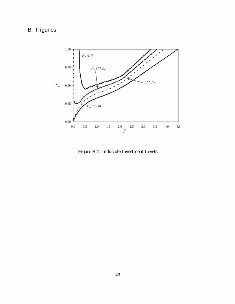
B. Figures

0.00

0.25

0.50

0.75

1.00

0.0 0.5 1.0 1.5 2.0 2.5 3.0 3.5 4.0 4.5

F m (1, β)

F m

β

F m (.75, β)

F m (.5, β )

F m (.25, β)

Figure B.1: Inducible Investment Levels

43

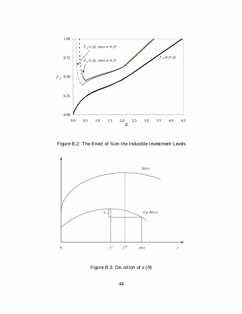
0.00

0.25

0.50

0.75

1.00

0.0 0.5 1.0 1.5 2.0 2.5 3.0 3.5 4.0 4.5

F m (0.25, β)

F m

β

F m (1, β), when σ=0.35

F m (1, β), when σ=0.25

Figure B.2: The E¤ect of ¾ on the Inducible Investment Levels

(1-μ )S(x)-x

S(x)-x

α

0 xw xFB x(α ) x

Figure B.3: De…nition of x (®)

44

References

Aghion, P., Dewatripont, M. and P. Rey. 1994. Renegotiation Design with Unveri…able

Information. Econometrica 62, 257-282.

Anderlini, L., L. Felli, and A. Postlewaite. 2001. Courts of Law and Unforeseen Contin-

gencies. Unpublished manuscript.

Ayres I. and R. Gertner. 1989. Filling Gaps in Incomplete Contracts: An Economic Theory

of Default Rules. Yale Law Journal 99, 87-130.

Bernardo, A., E. Talley, and I. Welch. 2000. A Theory of Legal Presumptions. Journal of

Law, Economics, and Organization 16, 1-49.

Bull, J. 2001a. Costly Evidence and Systems of Fact-…nding. Unpublished manuscript.

Bull, J. 2001b. Costly Evidence Production and the Limits of Veri…ability. Unpublished

manuscript.

Bull, J. and J. Watson. 2001. Evidence Disclosure and Veri…ability. Unpublished manuscript.

CALA (Citizens Against Lawsuit Abuse). 2002 (ed.). <http://www.cala.com/ cala10.htm>

Visited July 2002.

Che, Y. and T. Chung. 1999. Contract Damages and Cooperative Investment. Rand

Journal of Economics 30, 84-105.

Che Y. and D. Hausch. 1999. Cooperative Investment and the Value of Contracting.

American Economic Review 89, 125-147.

Coase, R. 2000. The Acquisition of Fisher Body by General Motors. Journal of Law and

Economics 43, 15-31.

Cooter R., and D. Rubinfeld. 1989. Economic Analysis of Legal Disputes and Their

Resolution. Journal of Economic Literature 27, 1067-1097.

45

DiCarlo, V. 2002. How Arbitration Can Protect Your Business from Ruinous Lawsuits.

<http://www.dicarlolaw.com/BusArbArt.htm.> Visited October 2002.

Daughety, A. and J. Reinganum. 2000. On the Economics of Trials: Adversarial Process,

Evidence, and Equilibrium Bias. Journal of Law, Economics, and Organization 16,

365-394.

De Fraja, G. 1999. After You Sir. Hold-Up, Direct Externalities, and Sequential Investment.

Games and Economic Behavior 26, 22-39.

Dewatripont, M. and E. Maskin. 1995. Contractual Contingencies and Renegotiation.

Rand Journal of Economics 26, 704-719.

Edlin A. 1996. Cadillac Contracts and Up Front Payments: E¢cient Investment under

Expectation Damages. Journal of Law, Economics, and Organization 12, 98-118.

Edlin A. and S. Reichelstein. 1996. Holdups, Standard Breach Remedies, and Optimal

Investment. American Economic Review 86, 478-501.

Eggleston, K., E. Posner and R. Zeckhauser. 2000. Simplicity and Complexity in Contracts.

John M. Olin Law & Economics Working Paper 93. University of Chicago.

Froeb, L. and B. Kobayashi. 2000. Evidence Production in Adversarial vs. Inquisitorial

Regimes. Vanderbilt University Law School Working Paper 99-13. Vanderbilt Univer-

sity.

Geis, G. and L. Bienen. 1998. Crimes of the Century: From Leopold and Loeb to O.J.

Simpson. (Boston: Northeastern University Press.)

Gong, J. and P. McAfee. 2000. Pretrial Negotiation, Litigation, and Procedural Rules.

Economic Inquiry 38, 218-238.

Grossman, S. and O. Hart. 1986. The Costs and Bene…ts of Ownership: A Theory of

Vertical and Lateral Integration. Journal of Political Economy 94, 691-719.

46

Grout, P. 1984. Investment and Wages in the Absence of Binding Contracts: A Nash

Bargaining Approach. Econometrica 52, 449-460.

Hart, O. and J. Moore. 1988. Incomplete Contracts and Renegotiation. Econometrica 56,

755-785.

Hart, O. and J. Moore. 1999. Unforeseen Contingencies and Incomplete Contracts. Review

of Economic Studies 66, 115-138.

Ishiguro, S. 1999. Incomplete Contracts and Breach Remedies. Journal of Institutional and

Theoretical Economics 155, 342-361.

Ishiguro, S. 2002. Endogenous Veri…ability and Optimality in Agency. Journal of Economic

Theory 105, 518-530.

Klein, B., R. Crawford and A. Alchian. 1978. Vertical Integration, Appropriable Rent, and

the Competitive Contracting Process. Journal of Law and Economics 21, 297-326.

Macaulay, S. 1985. An Empirical View of Contracts. Wisconsin Law Review (1985) 3,

465-482.

MacLeod, W. and J. Malcomson. 1993. Investment, Holdup, and the Form of Market

Contracts. American Economic Review 83, 811-837.

Mahoney, P. 1999. Contract Remedies: General. Encyclopedia of Law and Economics,

Chapter 4600.

Maskin, E. and Tirole, J. 1999. Unforeseen Contingencies and Incomplete Contracts. Re-

view of Economic Studies 66, 83-114.

Posner, E. 2002. Economic Analysis of Contract Law after Three Decades: Success or

Failure? John M. Olin Law & Economics Working Paper 146. University of Chicago.

Rogerson, W. 1992. Contractual Solutions to the Hold-Up Problem. Review of Economic

Studies 59, 774-794.

47

Rubinfeld, D. and D. Sappington. 1987. E¢cient Awards and Standards of Proof in Judicial

Proceedings. RAND Journal of Economics 18, 308-315.

Sanchirico, C. 1997. Evidence Production, Adversarial Process and the Private Investiga-

tion of Suits. Working Paper, Department of Economics, Columbia University.

Sanchirico, C. 2000. Games, Information, and Evidence Production with Application to

English Legal History. American Law and Economics Review 2, 342-380.

Schwartz, A. 1992. Relational Contracts in the Courts: An Analysis of Incomplete Agree-

ments and Judicial Strategies. Journal of Legal Studies 21, 271-318.

Schwartz, A. and R. Scott. 2002. Contract Theory and the Limits of Contract Law.

Unpublished manuscript.

Schwartz, A. and J. Watson. 2001. The Law and Economics of Costly Contracting. Un-

published manuscript.

Segal, I. and M. Whinston 2002. The Mirrlees Approach to Mechanism Design with Rene-

gotiation (with Applications to Hold-Up and Risk Sharing). Econometrica 70, 1-45.

Tirole, J. 1986. Procurement and Renegotiation. Journal of Political Economy 94, 235-259.

Tirole, J. 1999. Incomplete Contracts: Where do We Stand. Econometrica 67, 741-781.

Williamson, O. 1985. The Economic Institutions of Capitalism (New York: Free Press.)

Willington, M. 2002. A note on Ishiguro, 2002: Endogenous Veri…ability and Optimality

in Agency. Unpublished manuscript.

48

hold-up under costly litigation and imperfect courts of lawfm · hold-up under costly litigation...

Documents