holocene glacial history of renland, east greenland
TRANSCRIPT

The University of MaineDigitalCommons@UMaine
Electronic Theses and Dissertations Fogler Library
5-2013
Holocene Glacial History of Renland, EastGreenland Reconstructed From Lake SedimentsAaron Medford
Follow this and additional works at: http://digitalcommons.library.umaine.edu/etd
Part of the Climate Commons
This Open-Access Thesis is brought to you for free and open access by DigitalCommons@UMaine. It has been accepted for inclusion in ElectronicTheses and Dissertations by an authorized administrator of DigitalCommons@UMaine.
Recommended CitationMedford, Aaron, "Holocene Glacial History of Renland, East Greenland Reconstructed From Lake Sediments" (2013). ElectronicTheses and Dissertations. 1934.http://digitalcommons.library.umaine.edu/etd/1934

HOLOCENE GLACIAL HISTORY OF RENLAND, EAST GREENLAND
RECONSTRUCTED FROM LAKE SEDIMENTS
By
Aaron Medford
B.S. Lafayette College, 2011
A THESIS
Submitted in Partial Fulfillment of the
Requirements for the Degree of
Master of Science
(in Earth and Climate Sciences)
The Graduate School
The University of Maine
August 2013
Advisory Committee:
Brenda L. Hall, Professor, School of Earth and Climate Sciences and Climate
Change Institute, Advisor
George H. Denton, Professor, School of Earth and Climate Sciences and Climate
Change Institute
Daniel F. Belknap, Professor, School of Earth and Climate Sciences, Cooperating
Professor, Climate Change Institute
Ann C. Dieffenbacher-Krall, Assistant Research Professor, Climate Change
Institute

ii
THESIS ACCEPTANCE STATEMENT
On behalf of the Graduate Committee for Aaron Medford I affirm that this
manuscript is the final and accepted thesis. Signatures of all committee members are on
file with the Graduate School at the University of Maine, 42 Stodder Hall, Orono, Maine.
________________________________________________________________________
Dr. Brenda Hall, Professor of Sciences and Quaternary and Climate Studies 6/25/2013

LIBRARY RIGHTS STATEMENT
In presenting this thesis in partial fulfillment of the requirements for an advanced
degree at the University of Maine, I agree that the Library shall make it freely available
for inspection. I further agree that permission for “fair use” copying of this thesis for
scholarly purposes may be granted by the Librarian. It is understood that any copying or
publication of this thesis for financial gain shall not be allowed without my written
permission.
Signature:
Date:

HOLOCENE GLACIAL HISTORY OF RENLAND, EAST GREENLAND
RECONSTRUCTED FROM LAKE SEDIMENTS
By Aaron Medford
Thesis Advisor: Dr. Brenda L. Hall
An Abstract of the Thesis Presented
in Partial Fulfillment of the Requirements for the
Degree of Master of Science
(in Earth and Climate Sciences)
August 2013
The Arctic is responding to the modern increase in temperature, resulting in ice
loss and consequent sea-level rise. In order to understand present-day changes, we need
to understand how the Arctic has reacted in the past to natural variations in climate
forcing. To begin to identify the mechanisms behind climate change, I produced a
Holocene glacial and climate record for the Renland Ice Cap, Scoresby Sund, East
Greenland, from sediments in glacially fed lakes. I cored Rapids and Bunny Lakes, which
are fed by meltwater from the Renland Ice Cap, as well as Raven Lake, which does not
receive glacial influx at present. The presence or absence of glacial sediments in Rapids
and Bunny Lakes gives information on the size of the Renland Ice Cap.
I studied multiple sediment characteristics in the cores, including magnetic
susceptibility (MS), grain size, organic and carbonate content, and color intensity. In
general, I identified glacial sediment as grey, inorganic, and with high MS. Non-glacial

material was black or brown with high organic content and low MS. Chronology for the
cores came from radiocarbon dating of macrofossils and sieved organic fragments.
My results suggest that the region may have deglaciated as early as ~12.5 ka. The
high organic content in all three lakes suggests that the early- to mid-Holocene was warm
with periods of limited ice extent, consistent with the Holocene thermal maximum, which
has been documented elsewhere. After this warmth, the area cooled during the
Neoglaciation that culminated in the largest glacial event of the Holocene during the
Little Ice Age. Superimposed on the long-term climate change were multiple centennial-
to-millennial-scale glacial advances at ~ 9.4, 8.6-8.8, 8.1-8.3, 7.6-7.8, 7.0-7.5, 5.8-6.0,
4.7-5.0, 3.7-4.0, 3.0-3.6, and ~1.0 (AD 600 and 900) cal. kyBP.
My reconstruction of variations in the Renland Ice Cap matches well with other
glacial records from Scoresby Sund and from the wider Northern Hemisphere. In
addition, comparison with other glacial records from the Scoresby Sund region suggests
that elevation exerts a strong control on the timing, size, and number of glacial advances
exhibited at each site. This highlights the need for caution when comparing glacial
records from large geographic areas.
The Renland record, along with other Northern Hemisphere data, indicates
pervasive millennial-scale climate change throughout the Holocene, with the largest
magnitude glacial advance occurring during the Little Ice Age. This pattern favors a
cyclical forcing mechanism, such as solar variability or a 'wobbly ocean conveyor,' rather
than unique events, such as volcanic eruptions or outburst floods, as a cause of
millennial-scale climate change.

iii
ACKNOWLEDGMENTS
I would like to begin by thanking my advisor, Dr. Brenda Hall, for this great
opportunity, as well as for the guidance and knowledge she has passed on. I also want to
thank my committee Dr. George Denton, Dr. Daniel Belknap, and Dr. Ann
Dieffenbacher-Krall for their expertise and help in improving my thesis.
I owe the National Science Foundation, the University of Maine Graduate School
Government, and School of Earth and Climate Science for funding my master’s work.
Thank you to the School of Earth and Climate Science, the Climate Change Institute,
Dartmouth College, and the University of Minnesota Limnological Research Center for
the use of lab space and material. In addition, the work in Scoresby Sund, would not have
happened without the support of the late Gary Comer.
I was fortunate to join an ongoing project, and I am excited to add my record to
the already stellar work done by this group. I want to especially thank my field team Dr.
Brenda Hall, Dr. Meredith Kelly, Dr. Tom Lowell, Dr. Yarrow Axford, Paul Wilcox, and
Laura Levy for help in collecting and analysis of the data. In addition, I would like to
thank Krista Slemmons and Karen Marysdaughter for help in processing the cores.
I am grateful to my family for their support throughout the last two years, giving
me unconditional support. I would like to thank the faculty and staff in the Climate
Change Institute and School of Earth and Climate Sciences; it has been a great and
rewarding experience being able to work with you. I would like to thank my fellow
graduate students, especially the game night group, for support and encouragement.
Finally, I would like to acknowledge the geology department at Lafayette College, who
laid the foundation that allowed me to accomplish what I did.

iv
TABLE OF CONTENTS
ACKNOWLEDGMENTS............................................................................................
LIST OF TABLES.......................................................................................... ………
LIST OF FIGURES......................................................................................................
CHAPTER
1. INTRODUCTION………………………………………........................................
1.1 Overview…………………………………………………………………
1.2 Background……………………………………………………................
2. METHODS………………………………………………………………………...
2.1 Field Work………………………………………………………………..
2.2 Lab Work………………………………....................................................
3. RESULTS………………………………………………………………………….
3.1 Lake Setting………………………………………………………………
3.1.1 Glacial Lakes……………………………………………….......
3.1.2 Conceptual Model……………………………………………...
3.1.3 Non-Glacial Lake……………………………………................
3.2 Sediment Core Descriptions………………….…………………………..
3.2.1 Rapids Lake……………………….…………………................
3.2.1.1 RPD11-1B-1…………………………………………...
3..
3 3. 3
iii
vii
viii
1
1
4
7
7
10
16
16
16
23
26
31
31
31

v
3.2.2 Bunny Lake…………………………………….........................
3.2.2.1 Southern Basin: BNL11-1A-1………………................
3.2.2.2 Southern Basin: BNL11-1B-1........................................
…………………… 3.2.2.3 Northern Basin: BNL11-2A-1…………………………
3.2.2.4 Northern Basin: BNL11-2A-2…………………………
3.2.3 Raven Lake………………………….…………….....................
3.2.3.1 RAV11-1A-1…………………………………………..
3.2.3.2 RAV11-1A-2…………………………………………..
3.2.3.3 RAV11-2A-1…………………………………………..
3.2.3.4 RAV11-3A-1…………………………………………..
4. DISCUSSION ……………………………………........................……………….
4.1 Age Model………………………..............................................................
4.1.1 Radiocarbon Date Quality……………………………………...
4.1.2 Rapids Lake……………………..............................................
4.1.3 BNL11-1…………………………..............................................
4.1.4 BNL11-2………………………………......................................
4.1.5 Raven Lake……………………………….................................
4.2 Lake History……………………………………………………………...
4.2.1 Raven Lake……………………………………………………..
4.2.2 Rapids Lake………………………………….............................
4.2.3 Bunny Lake………………………………………….................
4.3 Glacial History of Raven, Rapids, Bunny Lake…………….....................
37
37
42
43
48
50
50
54
55
58
61
61
61
62
62
63
65
67
67
69
73
78

vi
4.4 Comparison of Climate Records…………………………………………
4.4.1 Comparisons between the Renland Glacial
Record and the Renland Ice Core ……………………………
4.4.2 Holocene Glacier and Climate Fluctuations in Greenland.……
4.4.3 Comparisons between the Glacial Record
and the GISP2 Ice Core………………………………………..
4.4.4 European Holocene Glacial and Climate Records……………..
4.4.5 North American Holocene Glacial and Climate Record……….
4.5 Holocene Climate Forcing…………………….........................................
5. CONCLUSIONS ………………………………………………………………….
REFERENCES……………………………………….................................................
APPENDIX A: DETAILED GRAIN SIZE MEASUREMENT METHOD…………
APPENDIX B: CORE LOGS…………...…………...................................................
BIOGRAPHY OF AUTHOR………..……………………………………………….
81
81
85
91
92
93
94
99
101
110
112
126

vii
LIST OF TABLES
Table 1 Basic information for each of the cored lakes…………………….................
Table 2 Radiocarbon samples………………………………………………………..
Table 3 Basic information on each of the cores..………………..………….………..
Table 4 Age model for master cores………………………………………................
Table 5 Timing of glacial advances of the Renland Ice Cap………………………...
9
13
18
65
75

viii
LIST OF FIGURES
Figure 1 ASTER image showing Scoresby Sund……………….................................
Figure 2 A detailed image of the study area………...………………………………..
Figure 3 Delta at southwest outlet of Large Lake (view to the southwest)…………..
Figure 4 Image of Rapids and Bunny Lakes (view to the northeast)………………...
Figure 5 Bathymetric map of Rapids Lake.………………………………………….
Figure 6 Aerial image of area surrounding Rapids and Bunny Lakes……………….
Figure 7 Bathymetric map of Bunny Lake………….………………………………..
Figure 8 Conceptual model of glacial input into Rapids and Bunny Lakes………….
Figure 9 Image of Raven Lake (view to the south)…………………….…………….
Figure 10 Bathymetric map of Raven Lake…………………………………….……
Figure 11 Aerial Image of the area surrounding Raven Lake…………………..........
Figure 12 Rapids Lake cores plotted by depth below water surface………………..
Figure 13 Radiocarbon dates for RPD11-1…………………………………………..
Figure 14 Data for RPD11-1, the master core for Rapids Lake……………………...
Figure 15 Bunny Lake cores plotted by depth below water surface………................
Figure 16 Radiocarbon dates for BNL11-1……………………………………….….
Figure 17 Data for BNL11-1, the master core for the south basin
in Bunny Lake……………………………………………………………..
Figure 18 Radiocarbon dates for BNL11-2…………………………………………..
Figure 19 Data for BNL11-2, the master core for the north basin
in Bunny Lake……………………………………………………………..
5
8
17
17
20
21
22
24
27
29
30
32
33
34
38
39
40
45
46

ix
Figure 20 Relationship between color intensity and percent organic material………
Figure 21 Raven Lake cores plotted by depth below water surface……….................
Figure 22 Radiocarbon dates for RAV11-1………………………………………….
Figure 23 Data for RAV11-1, the master core for Raven Lake……………………...
Figure 24 Radiocarbon dates for RAV11-2A-1……………………………………...
Figure 25 Data for RAV11-2A-1…………………………………………………….
Figure 26 Radiocarbon dates for RAV11-3A-1……………………………………...
Figure 27 Data for RAV11-3A-1…………………………………………………….
Figure 28 RPD11-1 age model……………………………………………………….
Figure 29 BNL11-1 age model…………………………………………….................
Figure 30 BNL11-2 age model……………………………………………………….
Figure 31 RAV11-1 age model……………………………………………................
Figure 32 Comparison with Greenland ice cores…………………………………….
Figure 33 Comparison of Holocene glacial margin records from the
Northern Hemisphere …………………………………………….……….
Figure 34 Initial description of core BNL11-1A-1…………………………………..
Figure 35 Initial description of core BNL11-1B-1…………………………………...
Figure 36 Initial description of core BNL11-2A-1…………………………….…….
Figure 37 Initial description of core BNL11-2A-2…………………………………..
Figure 38 Initial description of core BNL11-3A-1…………………………………..
Figure 39 Initial description of core RAV11-1A-1…………………………………..
Figure 40 Initial description of core RAV11-1A-2…………………………………..
Figure 41 Initial description of core RAV11-2A-1…………………………………..
47
51
52
53
56
57
59
60
64
64
66
66
82
87
112
113
114
115
116
117
118
119

x
Figure 42 Initial description of core RAV11-3A-1…………………………………..
Figure 43 Initial description of core RAV11-4A-1…………………………………..
Figure 44 Initial description of core RPD11-1A-1…………………………………...
Figure 45 Initial description of core RPD11-1B-1…………………………………...
Figure 46 Initial description of core RPD11-1C-1…………………………………...
Figure 47 Initial description of core RPD11-2A-1…………………………………...
120
121
122
123
124
125

1
CHAPTER 1
INTRODUCTION
1.1 Overview
Natural changes in forcing have produced significant variations in Earth’s climate
(Zachos et al., 2005). Arctic amplification, a process by which multiple feedbacks
strengthen the climate response to climate change, may allow northern polar regions to
react more quickly and to a larger degree to climate forcing than other parts of the globe
(e.g., Miller et al., 2010; Serreze and Barry, 2011; ACIA, 2005). The National
Aeronautics and Space Administration (NASA) surface temperature reconstruction
(Hansen et al., 2010) indicates that the Arctic has warmed among the most of any region
globally during the last 100 years, and the Arctic environment has begun to change in
response to these warmer temperatures. For example, sea-ice spatial extent and thickness
are decreasing (e.g., ACIA, 2005; Rothrock et al., 1999; Kwok et al., 2009; Chapman and
Walsh, 1993) at a rate faster than models have predicted (Stroeve et al., 2007). The
Greenland Ice Sheet (GIS) is thinning due to increased velocity and discharge of outlet
glaciers (e.g., Krabill et al., 2004; Howat et al., 2007; Stearns and Hamilton, 2007; Rignot
and Kanagaratnam, 2006). Moreover, additional processes linking seasonal surface melt
and ice-flow speed in the GIS suggest that the ice sheet will contribute more melt and
increase sea-level rise faster than previously predicted (Parizek and Alley, 2004; and
references within).
In order to help predict accurately how the Arctic and Greenland, specifically,
will respond to future change, both natural and anthropogenic, we need a complete
understanding of past climate variability. The Holocene (the past ~11,500 calendar years)

2
is a period of relatively stable interglacial climate (e.g., Bond et al., 1997; Fronval and
Jansen, 1997) upon which centennial- and millennial-scale climate anomalies are
superimposed. Hypotheses to account for these climate fluctuations include solar
variability (e.g., Bond et al., 2001; Denton and Karlén, 1973), ocean circulation (Denton
and Broecker, 2008), and increased volcanic activity (Miller et al., 2012). The climate in
the Holocene is important because modern human societies developed during this time.
In addition, it is the climate in which our society exists today. Therefore, climate shifts
during the Holocene, even small fluctuations, may have had a profound impact on the
growth and development of human societies. By creating a detailed climate record for the
Holocene, we can understand better the relationship between humans and climate.
One way to understand the causes of past climate change and to assess whether
current variations are unique, is to develop high-resolution temporal records over a
variety of scales and environments spanning the globe. By determining the spatial extent,
timing, and interhemispheric relationship of Holocene events, we can understand better
the initial forcing and feedbacks producing the observed climate shifts. Moreover,
because the Holocene is the most recent time period, most deposits from this time have
not been eroded, altered, or destroyed. Therefore, detailed and high-resolution climate
records from multiple proxies spanning the globe can be constructed. This detail will
allow for accurate identification of the response of the climate system and identification
of the forcing. East Greenland is a prime location to produce a detailed climate record,
because abundant glacial deposits there allow for a high-resolution record to be
constructed. The Renland Ice Cap has been drilled to bedrock, and the resulting local
climate record will allow for comparison with the climate record derived from changes in

3
the glacial margin. In addition, the region is optimally located to record variations in
circulation in the North Atlantic Ocean.
Previous work in the Scoresby Sund region of East Greenland (Fig. 1) indicates
that the largest spatial extent of glaciers in the Holocene was during the Little Ice Age
(LIA) (AD ~1150-1850) (e.g., Hall et al., 2008; Kelly et al., 2008; Lusas, 2011). Because
the LIA glacial advance surpassed the limits of older Holocene glaciations and thus
eroded or buried deposits from those time periods, the Holocene moraine record
commonly is limited and skewed heavily towards the youngest event. In order to develop
a record for the entire Holocene, I analyzed past glacier fluctuations from nearby lake
sediments, which are a complementary, continuous, high-resolution proxy. Lake
sediments have been used previously to reconstruct the Holocene glacial and climatic
record in Greenland (e.g., Larsen et al., 2011; Lusas, 2011; Wagner and Melles, 2002;
Kaplan et al., 2002; Cremer et al., 2001; Briner et al., 2010), and Scandinavia (e.g.,
Bakke et al., 2005; Dahl et al., 2003; Levy et al., submitted). One approach is to use a
threshold lake that receives glacial sediments only when the ice is large enough to surpass
a bedrock barrier and to contribute melt water into the watershed. In such situations, the
presence or absence of glacial sediment affords information on glacier size and proximity
to the lake. In addition, some researchers (e.g., Dahl et al., 2003; Nesje et al., 2001) also
have reconstructed ice fluctuations from lakes that always receive glacial meltwater.
Here, the principle is that the amount and grain size of glacial material increases as the
glacier nears the lake. In general, glacial sediments are inorganic, grey (for most rock
types), and clay-rich, as opposed to non-glacial sediments, which tend to be high in
organic material, brown or black in color, and silt rich.

4
Specifically, in this study my goals are to:
Constrain fluctuations of Renland Ice Cap throughout the Holocene to
produce a glacial and climate history;
Compare my high-resolution record to existing reconstructions of
Holocene climate change both in Greenland and worldwide;
Use multiple climate records to address questions concerning the forcing
and amplifications responsible for Holocene climate variability.
My specific objectives to address the goals posed above include:
Coring lakes that receive meltwater and sediment from the Renland Ice
Cap, as well as a non-glacially fed control lake in the same region;
Analyzing the cores using multiple proxies, including stratigraphy, loss-
on-ignition, magnetic susceptibility, and grain size;
Interpreting the data in terms of glacial size and presence/absence;
Studying aerial photography, satellite images, and ground observations to
identify geomorphic features to help constrain glacial history of region.
1.2 Background
Scoresby Sund (~69-72˚N, 21-30˚W) trends west-east and is the largest fjord
system on the east coast of Greenland (Fig. 1). It drains the Greenland Ice Sheet (GIS)
into the North Atlantic. Isolated, independent ice caps and mountain glaciers cover the

5
F
igure
1:
AS
TE
R i
mag
e sh
ow
ing S
core
sby S
und. T
his
stu
dy i
s par
t of
a la
rger
pro
ject
to o
bta
in g
laci
al r
ecord
s fr
om
Sco
resb
y
Sund, i
ncl
udin
g M
ilne
Lan
d (
Lev
y e
t al
., i
n r
evie
w),
Gra
ben
Lan
d (
Wil
cox, 2013),
and L
iver
pool
Lan
d (
inse
t) (
Lo
wel
l et
al.
, 2013;
Lusa
s, 2
011).
My s
tudy a
rea
is o
utl
ined
by t
he
purp
le b
ox o
n t
he
south
wes
tern
mar
gin
of
Ren
land I
ce C
ap.

6
plateaus and mountain chains of the region. Renland (~70.5-71.5˚N, 24-28˚W) (Fig. 1),
the focus of this study, is a plateau rising as high as 2340 m elevation, with a gently
undulating topography. It is underlain mostly by granite and paragneisses from the
Caledonian orogeny (Leslie and Nutman, 2000). At present, a small ice cap (1200 km2) a
few hundred meters thick (Johnsen et al., 1992) covers most of Renland. Evidence
suggests that the ice cap has remained isolated from the GIS, even during the Last Glacial
Maximum (LGM) (Johnsen et al., 1992). I chose to study Renland, in part, because the
ice cap has been cored to bedrock and has a climate record that extends into the Eemian
interglacial (Johnsen et al., 1992). The Holocene is well preserved in this core (Johnsen et
al., 1992), which allows a detailed comparison with the lake records developed herein.
Previous studies suggest that glacier size is related largely to summer temperature,
whereas temperature proxies from the Greenland ice cores represent conditions over a
full year (Koerner, 2005; Denton et al., 2005). Thus, the proximity of the Renland ice
core to my field area allows for comparison of average yearly conditions from the ice
core and summer temperatures from glacier fluctuations as derived from lake sediments.
Denton et al. (2005) used this type of comparison to help determine climate seasonality in
the region during the Younger Dryas.

7
CHAPTER 2
METHODS
2.1 Field Work
I identified potential lakes through detailed study of aerial photographs and
satellite images. An ideal field area should have multiple glacially fed lakes, at least one
non-glacially fed lake (as a control), and only a single glacier contributing melt water to
the watershed. Furthermore, the lake preferably should have high organic productivity, so
that when the glacial signal is absent there is a large contrast between the two types of
depositional environments (Dahl et al., 2003). In August 2011, I retrieved sediment cores
from lakes in Renland that met most of these characteristics. The studied lakes most
likely receive glacial material from more than one glacier during the Holocene, which I
discuss in more detail in the conceptual model section. First, our field team constructed a
bathymetric map for each lake to identify the optimal coring location. We measured
depths by crossing the lake multiple times on a zodiac with a Humminbird device. We
used Dr. Depth (http://www.drdepth.se/), a sea-bottom mapping software, to analyze the
data. Paul Wilcox of the University of Cincinnati produced the final bathymetric maps.
We chose coring locations on the basis of depth, as well as on the surrounding
topography, and preferentially selected deep, flat basins.
The field team cored three lakes in Renland, two of which were glacially fed
(Rapids Lake and Bunny Lake) (Fig. 2), and one of which was non-glacial (Raven Lake)
(Table 1). Although Raven Lake does not receive glacial sediment at present, there are
abandoned channels feeding into the lake that head near a faint drift limit just distal to a
prominent LIA drift edge. Bunny and Rapids Lakes are a part of a chain of lakes. The

8
F
igure
2:
A d
etai
led i
mag
e of
the
study
are
a. A
t p
rese
nt,
Lar
ge
Lak
e is
dam
med
to t
he
nort
hea
st b
y o
utl
et g
laci
ers
of
Ren
lan
d I
ce C
ap
and a
sm
all
ice
cap t
o t
he
south
and f
low
s th
rough a
bed
rock
outl
et t
o t
he
south
wes
t in
to a
ser
ies
of
bed
rock
-flo
ore
d s
trea
ms
and l
akes
.
We
core
d t
wo o
f th
ose
lak
es, R
apid
s an
d B
unny, as
wel
l as
a t
hir
d l
ake,
Rav
en, w
hic
h d
oes
not
rece
ive
gla
cial
sed
imen
t at
pre
sent.
A
larg
e del
ta i
s bei
ng b
uil
t onto
the
outl
et o
f L
arge
Lak
e fr
om
a m
eltw
ater
str
eam
flo
win
g f
rom
Ren
land I
ce C
ap.

9
glacial signal in these lakes is controlled by the size and outflow of Large Lake (informal
name) at the head of this chain. The size of this first lake is a function of the amount of
glacial melt water and the position of ice-cap outlet glaciers that, at times, terminate in
the lake.
The coring platform was formed from two zodiac boats joined by a metal “A”
frame. We used a modified Bolivian coring system (Myrbro and Wright, 2008) to retrieve
the sediment cores. We lowered the polycarbonate tube (1.5 m in length, 7.6 cm
diameter) by a wire from our platform. The wire could be replaced with screw-on metal
rods in water depths <15 m. When we reached the depth to start coring, we tied off the
piston and began to hammer the tubing down by raising and then dropping a weight. The
whole corer was pulled up by the wire (or rods), and before the bottom of the tube was
removed from the water, it was capped and then sealed with electrical tape. Any excess
tubing was cut off, and Zorbitrol preserved the sediment-water interface. The top was
then capped and sealed. We shipped cores to the Limnological Research Center (LRC) at
the University of Minnesota.
Table 1: Basic information for each of the cored lakes.
Lake Core Prefix Latitude Longitude Elevation
(m)
Max.
Depth
(m)
Type
Rapids
Lake RPD11 71.032483 27.41535 824 30
Glacially
Fed
Bunny
Lake BNL11 71.031183 27.42675 819 14
Glacially
Fed
Raven Lake RAV11 71.06601 27.31106 1054 20 Control

10
Cores were named using the following convention:
PFX11-MX-N
PFX=Prefix of cored lake
“11” indicates that cores were collected in 2011.
M= Site number. Sites are typically delineated by changing anchor locations
X =Hole letter. A different letter represents the boat was moved a few meters
without changing the anchor location.
N=Thrust number.
2.2 Lab Work
At the LRC, I used a Geotek Multisensor Core Logger to analyze whole cores,
measuring sediment density, acoustic wave velocity, electrical resistivity, and magnetic
susceptibility (MS) at approximately five-centimeter resolution. I then split and cleaned
each core and archived half at the LRC. With a Geotek XYZ Core Scanner, I measured a
higher-resolution MS record (0.5 cm) for each core. DMT CoreScan Colour captured
high-resolution digital images (10 pixels/mm). In addition, I performed a first-order
stratigraphic analysis, along with preliminary correlations of cores taken from the same
lake.
Following preliminary analysis at the LRC, I shipped the cores overnight to the
University of Maine and placed them in cool storage. I established a master core for each
lake to focus the analysis. The ideal master core included the longest sediment record,
contained the most sediment, had easy-to-identify tie points between core segments, and

11
was composed of the minimum number of segments necessary to cover the entire
stratigraphic record.
After each master core was constructed, I analyzed them in detail. I sampled for
radiocarbon dating with the focus on bracketing distinct changes in sediment type. I also
spaced samples along the length of the core. I collected two types of samples. Initially, I
took samples of macro-scale organic material, such as algae or leaves. I preferred
macrofossils to all other sample types. These samples were washed with deionized (DI)
water to remove sediment. If no macrofossils were present, I looked for organic-rich
layers. I sieved sediment from such layers through a 63 μm mesh using DI water. This
process concentrated any organic material. If macrofossils could be seen, I removed them
using tweezers. If none were present, I dated the concentrated organic material. After the
radiocarbon samples were taken, I placed them in a ~50°C oven until dry and then sent
them to The National Ocean Sciences Accelerator Mass Spectrometry (NOSAMS)
facility for analysis.
I calibrated the radiocarbon dates using CALIB v.6.1.0 (Stuiver and Reimer,
1993) and the INTCAL09 data set (Reimer et al., 2009). I assumed that any reservoir
effect is negligible because of the presumed low residency time of water in these lakes
and the absence of carbonate bedrock in the watershed. Lusas (2011) obtained a modern
age from aquatic algae at the sediment-water interface of Emerald Lake, which has
characteristics similar to lakes used in this study and which is also in the Scoresby Sund
region. Ages are presented as the mean value of the 2σ age range and are reported as
calibrated years before present (cal. yBP) with an associated 2σ error (Table 2). If there
were multiple possible calibrated ranges, that with the highest probability was used in the

12
text and to construct age models. I present all possible age ranges above ten percent
confidence in Table 2, and the majority of samples used in the age models have a
confidence over eighty-five percent.
Following methods outlined in Bengtsson and Enell (1986), I performed loss-on-
ignition (percent organic content) and percent carbonate analysis on the cores. The
percent carbonate value potentially also could reflect clays losing water in the mineral
structure. However, for simplicity I will refer to this value as percent carbonate
throughout the rest of the paper. I also performed grain-size analysis based on procedures
developed at Northern Arizona University’s Sedimentary Records of Environmental
Change Lab for preparing samples for a Coulter counter. I present a detailed description
in Appendix A. I took samples for both types of analyses at two-centimeter intervals.

13
Tab
le 2
: R
adio
carb
on s
ample
s. D
ates
wer
e ca
libra
ted w
ith C
AL
IB 6
.1.
OS
-95595
B
NL
-11-1
A-1
13
Sie
ved
425
40
-26.6
15
350
26
1600
AD
85
481
53
1470
AD
OS
-96874
BN
L11-1
A-1
27.4
Macro
1150
30
-30.8
96
1062
85
889
AD
OS
-96906
BN
L11-1
A-1
51
Sie
ved
2910
25
-31.7
77
3023
61
1074
BC
23
3273
185
1174
BC
OS
-95587
BN
L-1
1-1
A-1
97
Sie
ved
6380
30
-25.0
70
7298
40
5349
BC
30
7384
34
5435
BC
OS
-95586
BN
L-1
1-1
B-1
56
Sie
ved
6290
40
-29.7
100
7237
80
5288
BC
OS
-95640
BN
L-1
1-1
B-1
77
Macro
7170
50
-24.6
89
7994
67
6045
BC
OS
-100375
BN
L11-2
A-1
4M
acro
280
20
-24.2
50
307
19
1644
AD
49
402
27
1548
AD
OS
-100376
BN
L11-2
A-1
27.8
Sie
ved
1440
25
-32.8
100
1337
38
613
AD
OS
-100377
BN
L11-2
A-1
19
Sie
ved
1460
20
-31.7
100
1346
39
605
AD
OS
-100378
BN
L11-2
A-1
50.5
Sie
ved
3400
40
-31.0
93
3642
86
1693
BC
OS
-100379
BN
L11-2
A-1
60
Sie
ved
3280
30
-32.6
99
3511
68
1562
BC
OS
-100380
BN
L11-2
A-1
64
Sie
ved
3670
30
-33.5
100
3997
91
2048
BC
OS
-100381
BN
L11-2
A-1
65
Sie
ved
3480
30
-32.7
97
3762
76
1813
BC
OS
-100382
BN
L11-2
A-1
76.5
Sie
ved
3430
30
-32.9
81
3670
60
1721
BC
12
3808
18
1859
BC
cal.
yB
P
Err
or
(2 σ
)
Cal A
ge
(AD
/BC
)
δ13
C
(per
mil)
Confi
dence
(perc
ent)
Err
or
(1σ)
IDC
ore
Depth
:
Belo
w S
tart
of
Sed.
(cm
)
Sam
ple
Type
Radio
carb
on
Age (
14C
yB
P)

14
Tab
le 2
: C
onti
nued
OS
-100516
BN
L11-2
A-1
77
Sie
ved
4410
30
-34.4
95
4960
94
3011
BC
OS
-100517
BN
L11-2
A-1
96
Sie
ved
5250
30
-34.2
66
5978
53
4029
BC
18
6098
22
4149
BC
10
6163
14
4214
BC
OS
-100777
BN
L11-2
A-1
104
Sie
ved
6520
35
-28.7
87344
16
5395
BC
86
7459
46
5510
BC
OS
-100518
BN
L11-2
A-2
3S
ieved
6450
30
-29.0
100
7370
58
5421
BC
OS
-100519
BN
L11-2
A-2
9.5
Sie
ved
6710
30
-28.6
20
7532
23
5578
BC
78
7589
33
5640
BC
OS
-100520
BN
L11-2
A-2
15
Sie
ved
7300
35
-29.9
100
8101
76
6152
BC
OS
-100521
BN
L11-2
A-2
22.5
Sie
ved
7470
35
-30.2
43
8234
36
6285
BC
57
8323
48
6374
BC
OS
-100778
BN
L11-2
A-2
26
Sie
ved
7960
40
-31.8
94
8841
150
6892
BC
OS
-100522
BN
L11-2
A-2
29.5
Sie
ved
7870
35
-29.8
97
8678
100
6729
BC
OS
-100779
BN
L11-2
A-2
33
Sie
ved
8500
50
-30.1
100
9494
51
7545
BC
OS
-96048
RP
D11-1
B-1
5M
acro
960
20
-23.1
66
835
39
1116
AD
34
912
17
1038
AD
IDC
ore
Depth
:
Belo
w S
tart
of
Sed.
(cm
)
Sam
ple
Type
Radio
carb
on
Age (
14C
yB
P)
cal.
yB
P
Err
or
(2 σ
)
Cal A
ge
(AD
/BC
)
Err
or
(1σ)
δ13
C
(per
mil)
Confi
dence
(perc
ent)

15
Tab
le 2
: C
onti
nued
OS
-96047
RP
D11-1
B-1
17.5
Macro
200
20
-25.2
18
77
1944
AD
47
168
22
1783
AD
26
282
14
1668
AD
OS
-96058
RP
D11-1
B-1
21
Macro
250
25
-26.5
20
161
10
1789
AD
70
299
19
1651
AD
OS
-96045
RP
D11-1
B-1
39
Sie
ved
1990
25
-24.5
100
1940
53
10
AD
OS
-95933
RP
D11-1
B-1
99
Macro
7330
55
-24.1
90
8115
103
6166
BC
OS
-95567
RA
V11-1
A-1
9S
ieved
1080
35
-25.0
100
994
62
956
AD
OS
-96907
RA
V11-1
A-1
24
Sie
ved
1890
25
-32.1
94
1831
60
119
AD
OS
-95590
RA
V11-1
A-1
56
Macro
3660
30
-29.5
100
3992
92
2043
BC
OS
-96908
RA
V11-1
A-1
108
Sie
ved
5300
35
-30.7
98
6088
99
4139
BC
OS
-96909
RA
V11-1
A-1
125.8
Sie
ved
5740
40
-31.2
100
6541
102
4592
BC
OS
-95588
RA
V11-1
A-2
4S
ieved
5880
30
-30.4
97
6697
57
4748
BC
OS
-95589
RA
V11-1
A-2
11
Sie
ved
6960
35
-28.6
96
7778
85
5829
BC
OS
-95566
RA
V11-2
A-1
9S
ieved
5250
45
-30.4
87
6022
102
4073
BC
13
6162
18
4213
BC
OS
-95569
RA
V11-2
A-1
71
Sie
ved
8180
50
-27.7
19145
132
7196
BC
OS
-100776
RA
V11-3
A-1
17
Sie
ved
10650
55
-29.9
96
12614
89
10665
BC
IDC
ore
Depth
:
Belo
w S
tart
of
Sed.
(cm
)
Sam
ple
Type
Radio
carb
on
Age (
14C
yB
P)
Cal A
ge
(AD
/BC
)
Err
or
(1σ)
δ13
C
(per
mil)
Confi
dence
(perc
ent)
cal.
yB
P
Err
or
(2 σ
)

16
CHAPTER 3
RESULTS
Our field team retrieved approximately 12.5 m of sediment, with 447 cm in total
length (five cores) from Bunny Lake, 471 cm (five cores) from Raven Lake and 330 cm
(four cores) from Rapids Lake (Table 3). An initial core description performed at the
LRC is provided in Appendix B for every core.
3.1 Lake Setting
3.1.1 Glacial Lakes
Large Lake receives meltwater predominantly from the Renland Ice Cap, as well
as a lesser amount from a small ice cap to the south. Large Lake currently drains to the
southwest through a series of shallow, turbulent bedrock-floored streams and lakes. It is
dammed on the north-east end by a confluence of different outlet glaciers from the
Renland Ice Cap, and the ice cap to the south. If the dam were removed, the lake would
drain to the northeast and the southwest outlet might be abandoned. An incised channel
that heads at the Renland Ice Cap margin enters Large Lake at the west end and is
building a large delta that partially blocks the outlet. The delta is positioned so the
meltwater is able to flow both into Large Lake, as well as directly into the outlet stream
to the south-west (Fig. 3).
We cored two lakes, Rapids and Bunny (Fig. 4), along the stream that exits Large
Lake. Meltwater enters Rapids Lake through rapids and a waterfall. The current is
confined to the southern edge of the lake and exits to the southwest in a shallow stream
which then flows into Bunny Lake.
17
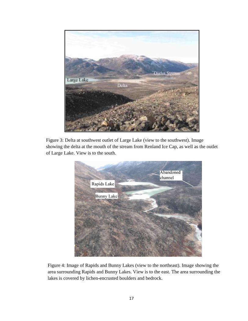
Figure 3: Delta at southwest outlet of Large Lake (view to the southwest). Image
showing the delta at the mouth of the stream from Renland Ice Cap, as well as the outlet
of Large Lake. View is to the south.
Figure 4: Image of Rapids and Bunny Lakes (view to the northeast). Image showing the
area surrounding Rapids and Bunny Lakes. View is to the east. The area surrounding the
lakes is covered by lichen-encrusted boulders and bedrock.

18
Tab
le 3
: B
asic
info
rmat
ion o
n e
ach o
f th
e co
res.
Rap
ids
Lak
e8/2
9/2
011
RP
D11-1
A-1
24.4
71.0
3248
27.4
1535
824
1.2
0-0
.21.0
Rap
ids
Lak
e8/2
9/2
011
RP
D11-1
C-1
24.4
71.0
3248
27.4
1535
824
0.7
0-0
.20.5
Rap
ids
Lak
e8/2
9/2
011
RP
D11-2
A-1
18
71.0
3307
27.4
133
819
1.0
0-0
.20.8
Rap
ids
Lak
e8/2
9/2
011
RP
D11-2
B-1
18
71.0
3307
27.4
133
819
0.4
0-0
.10.3
Bun
ny L
ake
8/3
0/2
011
BN
L11-1
A-1
11.4
71.0
3118
27.4
2675
819
1.1
5-0
.21.0
Bun
ny L
ake
8/3
0/2
011
BN
L11-1
B-1
11.4
71.0
3118
27.4
2675
819
1.4
40.2
1.6
Bun
ny L
ake
8/3
0/2
011
BN
L11-2
A-1
10.1
71.0
3233
27.4
2822
823
1.3
0-0
.21.1
Bun
ny L
ake
8/3
0/2
011
BN
L11-2
A-2
10.1
71.0
3233
27.4
2822
823
0.5
01.3
1.8
Bun
ny L
ake
8/3
0/2
011
BN
L11-3
A-1
10.1
71.0
3233
27.4
2822
823
0.6
00.9
1.5
Rav
en L
ake
8/2
6/2
011
RA
V11-1
A-1
15.5
71.0
6601
27.3
1106
1054
1.5
6-0
.11.4
Rav
en L
ake
8/2
6/2
011
RA
V11-1
A-2
15.5
71.0
6601
27.3
1106
1054
0.7
01.6
2.3
Rav
en L
ake
8/2
6/2
011
RA
V11-2
A-1
15.5
71.0
6601
27.3
1106
1054
0.9
31.3
2.2
Rav
en L
ake
8/2
6/2
011
RA
V11-3
A-1
15.6
71.0
6601
27.3
1106
1054
0.8
31.9
2.7
Rav
en L
ake
8/2
6/2
011
RA
V11-4
A-1
15.6
71.0
6601
27.3
1106
1054
0.8
81.2
2.1
Dep
th o
f C
ore
Top b
elow
Sed
. S
urfa
ce
Dep
th o
f C
ore
Bottom
bel
ow
sedim
ent su
rfac
e
Dat
e
Colle
cted
Lak
eC
ore
Nam
eL
atitu
de
Long
itude
Wat
er
Dep
th
(m)
Ele
vatio
n
(m)
Core
Len
gth
(m)

19
Rapids Lake is composed of a single steep-sided basin that reaches ~30 m depth (Fig. 5).
It is surrounded by steep topography that shows evidence of mass movement, including a
rockfall scar. The area surrounding the lake is covered by predominantly large, lichen-
covered boulders set in a sandy matrix. The lichen-covered boulders suggests a relative
stable slope that allows for lichen growth (Fig. 6).
Rapids Lake is separated from Bunny Lake by large ridges of uncertain origin.
The overall feature has approximately 10 m of relief with multiple, closely spaced ridges
each with 2 m relief composing the crest. Large lichen-covered boulders make up the
dominant grain size on the surface. A partial reindeer skeleton was found within the
deposit. This landform may represent a moraine complex, till-covered bedrock, or a large
mass movement deposit. There is insufficient evidence to eliminate any of these
hypotheses.
Bunny Lake (Fig. 7) has two major basins. The stream current flows through the
deeper (~14 m) southern basin (Fig. 7) and exits to the northeast. The northern basin is
slightly shallower (~10 m) and is removed from the current.
Bunny Lake is surrounded by steep slopes that display highly weathered, lichen-
encrusted till and exposed bedrock slopes. There is evidence of past mass movements on
these slopes. An abandoned stream channel enters the lake from a plateau to the south.
Both this plateau and a similar one to the north are lichen-free in satellite imagery. This
suggests that small ice caps or snowbanks were present on both plateaus in the recent
past. Thus, this channel is a potential source of sediment into Bunny Lake, although it is
likely to be small compared to that delivered from the river.

20
Figure 5: Bathymetric map of Rapids Lake. Image created by Paul Wilcox of the
University of Cincinnati. Color scale represents depth in meters below lake surface.
Second Scale represents horizontal distance. The black arrows indicate the inlet and
outlet for the lake.

21
Figure 6: Aerial image of the area surrounding Rapids and Bunny Lakes. Geomorphic
features indicated.

22
Figure 7: Bathymetric map of Bunny Lake. Image created by Paul Wilcox of the
University of Cincinnati. Color scale represents depth in meters below lake surface.
Second Scale represents horizontal distance. The black arrows indicate the inlet and
outlet for the lake.

23
3.1.2 Conceptual Model
Glacial silt in Rapids and Bunny Lake is derived from overflow from Large Lake,
which is fed by both outlet glaciers that terminate in the lake and by meltwater channels
that extend from the surrounding ice caps (Fig. 8). Even if the outlet glaciers were to
experience a modest retreat, the meltwater channels, particularly the large channel
extending from Renland Ice Cap to the delta at the west end of the lake, still would
contribute meltwater to the lake. Therefore, when Bunny and Rapids Lake lack glacial
sediments, Large Lake, as well as any meltwater channels, must be cut off from the chain
of lakes that include Bunny and Raven Lake.
A major control on Large Lake is the behavior of the surrounding glaciers. At
present, expanded glaciers dam the lake to the northeast, causing drainage to be through
the western outlet into Bunny and Rapids Lakes. If the lake were not dammed by ice,
water likely would flow to the northeast due to the slope of the topography. Thus,
overflow of silt-laden meltwater to the west and into Bunny and Rapids Lake is a
function of the presence or absence of the ice dam, not necessarily the volume of
meltwater produced by the Renland Ice Cap.
Ultimately, the record produced in this study records the size of the Renland Ice
Cap and the adjacent ice cap to the south. In particular, the presence of glacial sediments
in Bunny and Rapids Lakes reflect times when the ice caps were sufficiently large to
produce an ice dam on the northeast end of Large Lake. The ice dam controls the size of
Large Lake, and therefore, whether or not the lake drains over the western bedrock outlet
into Bunny and Rapids Lakes. When Large Lake can drain into Bunny and Rapids Lake,
the sedimentation in both lakes is swamped by the glacial influx.

24
Fig
ure
8:
Conce
ptu
al m
odel
of
gla
cial
input
into
Rap
ids
and B
unny L
akes
. A
bas
ic m
odel
show
ing t
hre
e key
tim
e p
erio
ds.
Duri
ng
max
imum
Holo
cene
exte
nt
(LIA
), o
utl
et g
laci
ers
from
Ren
land I
ce C
ap a
nd
the
smal
l ic
e ca
p t
o t
he
south
dam
med
Lar
ge
Lak
e,
whic
h o
ver
flow
ed t
o t
he
south
wes
t. E
xpan
ded
and
new
gla
cier
s ar
e dep
icte
d w
ith g
rey c
olo
r. I
n a
ddit
ion, sm
all
ice
caps
or
snow
ban
ks
on t
he
pla
teau
s nort
h a
nd s
outh
of
Rap
ids
and B
unny L
akes
may
hav
e co
ntr
ibute
d g
laci
al s
edim
ent
to t
hes
e la
kes
. T
hes
e
pla
teau
s ar
e not
snow
-co
ver
ed a
t p
rese
nt.
T
od
ay,
gla
cial
sed
imen
t re
aches
Bunny a
nd R
apid
s L
akes
bec
ause
of
over
flow
fro
m L
arge
Lak
e, a
nd t
o a
les
ser
exte
nt
bec
ause
of
a m
eltw
ater
str
eam
fro
m R
enla
nd I
ce C
ap. D
uri
ng t
he
Holo
cene
Ther
mal
Max
imum
(H
TM
),
ice
cap r
etre
at (
dott
ed l
ines
rep
rese
nt
smal
ler
gla
cier
s) l
ikel
y a
llow
ed L
arge
Lak
e to
dra
in t
o t
he
nort
hea
st. T
he
lack
of
ob
vio
us
gla
cial
sed
imen
t th
rough
out
much
of
this
tim
e per
iod i
n c
ore
s fr
om
Rap
ids
and B
unny L
akes
sugges
ts t
hat
the
mel
twat
er s
trea
m f
rom
Ren
land I
ce C
ap t
od
ay t
hat
form
s th
e del
ta a
t th
e w
est
end o
f L
arge
Lak
e ei
ther
als
o d
rain
ed t
o t
he
nort
hea
st o
r w
as i
nac
tive.

25

26
Because the ice dam may take some time to form, the appearance of glacial
sediment in Bunny and Rapids Lakes may be delayed compared to the time when the
climate first cools and the glaciers begin to advance. The ice dam may fail multiple times
during its initial formation before it becomes stable and large enough to confine Large
Lake and allow it to increase to a level where it will overflow to the west. Once built, the
ice dam should be stable, because the bedrock outlet should control the size of the lake.
This presents the lake from rising to a high level where it would float the dam. During
deglaciation, as climate begins to warm, the dam may weaken to a point where the lake
breaks through, causing a catastrophic drainage.
The plateaus on either side of Bunny and Rapids Lakes are a second potential
source of glacial sediments. Lichen-free areas indicate recent cover by ice or snow. If
these ice masses became sufficiently large, they may have contributed meltwater into
Rapids and Bunny Lakes through the now abandoned channels that head on the plateau.
3.1.3 Non-Glacial Lake
Raven Lake (Fig. 9) has an expansive, relatively flat bottom with two minor
basins, the deepest of which reaches ~20 m (Fig. 10). The southwestern section of the
lake is extremely shallow, less than one meter deep, and we did not create a bathymetric
map of that portion.
There was only minor outflow from the lake during our field expedition, and this
occurred as seep through a boulder-filled channel to the south (Fig. 11). The only obvious
inflow to the lake is through a groundwater-fed channel at the eastern edge of the lake.

27
This is sufficient to be forming a small delta. However, an increase in lake level of less
than a meter would reverse this water-flow direction and create a second outlet to the
southeast. A former spillway is cut into bedrock at the western end of the lake at 1064
masl, ~14 m above current lake level.
Glacial meltwater does not flow into the lake at present. However, an abandoned
channel enters the northeast end of the lake and heads just distal to the LIA drift limit
adjacent to Renland Ice Cap. However, because of the angularity of the boulders and the
abundance of precariously perched and weathered talus in the channel, it appears that the
channel has been inactive for a long time. A second channel enters the lake from the
north and is incised into till. This channel heads in the highlands between the Renland Ice
Cap and Raven Lake and does not appear to have been active for a long time. There is no
obvious water source. This abandoned channel features two deposits of well-sorted sand,
Figure 9: Image of Raven Lake (view to the south). Image showing the area surrounding
Raven Lake. View is to the south. The area is covered predominantly by lichen-encrusted
boulders. Note tents for scale.

28
each with five of meters relief. The upper sediments occur in flat-lying layer, which
overlie dipping beds. The sand is in contrast to the large lichen-covered boulders that
compose the surrounding drift. I infer that these sand deposits are deltas. These deltas
occur at about 14 m above present-day lake level, the same elevation as the former
bedrock spillway, and indicate a significantly higher lake level in the past, although their
age is not constrained. For these higher lake levels to have occurred, the lower outlets
must have been blocked by ice or by sediments. Thus, these features may date to early in
the deglacial period.
The terrain surrounding the lake is covered by with lichen-encrusted boulders in a
sandy matrix. I interpret this deposit as till. Till with such weathering elsewhere in the
Scoresby Sund region has yielded surface exposure ages of ~10-12 ka (Lowell et al.,
2013). In the valley east of the lake, the till forms multiple linear ridges, each with a few
meters in relief and spaced ~20 m apart; based on geometry, these rides are likely
moraines. A second set of more continuous ridges occurs approximately one kilometer
east in the same valley and has a relief of ~10 m. These ridges slope down to the
southeast. I infer that they also are moraines. Due to differences in orientation and scale,
the two sets may be of different age. There are also ridges near the groundwater inlet at
the southeast end of the lake. These are segmented and somewhat chaotic, but the overall
orientation is across the valley. A small-scale, roughly circular depression a few meters

29
F
igure
10:
Bat
hym
etri
c m
ap o
f R
aven
Lak
e. I
mag
e cr
eate
d b
y P
aul
Wil
cox o
f th
e U
niv
ersi
ty o
f C
inci
nnat
i. C
olo
r sc
ale
repre
sents
dep
th i
n m
eter
s bel
ow
lak
e su
rfac
e. S
econ
d S
cale
rep
rese
nts
ho
rizo
nta
l dis
tance
.

30
F
igure
11:
Aer
ial
imag
e of
the
area
surr
ou
ndin
g R
aven
Lak
e . G
eom
orp
hic
fea
ture
s in
dic
ated
.

31
deep may be a kettle. On the opposite side of the valley, close to lake level, there are
multiple hills with a few meters in relief that are composed predominantly of sand and
gravel with a few large boulders. All of these features may represent ice-recession or
stagnation features.
On the east slope of the same valley, there is a large deposit (~20 m of relief) with
a steep front and a broad flat top is composed of large, lichen-covered boulders. Based on
its form and composition, this deposit is a relict rock glacier (Martin and Whalley, 1987).
3.2 Sediment Core Descriptions
3.2.1 Rapids Lake
We took four cores from Rapids Lake (Table 3, Fig.12). Because they all show
the same stratigraphy, I chose the longest record, RPD11-1B-1, as the master core (Fig.
13, 14).
3.2.1.1 RPD11-1B-1
From the base of the sediments (112 cm depth) to 83 cm depth, RPD11-1B-1 is
composed of a laminated black (10 YR 2/1) clayey-silt (Fig. 13, 14). Coarser reddish-
gray (2.5 YR 6/1) layers of clayey-silt punctuate the darker clayey silt at 101-104, 90, 89,
and 83 cm depth. Two massive reddish-gray fine sand layers with black flecks also occur
at 98-99 and 94-9 cm depth.
The laminated black clayey silt is overlain abruptly by a very finely laminated
dark brown clayey-silt at 83 cm depth. This unit is 46 cm thick with laminations
(approximately 0.1 cm thick) that vary slightly in color with the predominant color being

32
Figure 12: Rapids Lake cores plotted by depth below water surface. Ages of radiocarbon
dates are given in cal. yBP. Black lines between cores show tie points, and blue lines
show the sediment-water interface. Note change of scale for RPD11-2A-1.

33
Figure 13: Radiocarbon dates for RPD11-1. The grey number is out of
stratigraphic order and is omitted from further discussion.

34
F
igure
14:
Dat
a fo
r R
PD
11
-1, th
e m
aste
r co
re f
or
Rap
ids
Lak
e. A
ges
wer
e ca
lcula
ted w
ith t
he
age
model
. Y
-axis
tic
k m
arks
rela
te t
o
dep
th. T
he
firs
t gra
in s
ize
pan
el s
how
s dat
a m
easu
red o
n a
Coult
er C
ounte
r, w
her
eas
that
in t
he
stra
tigra
phic
colu
mn w
as b
ased
on
vis
ual
obse
rvat
ion. T
he
firs
t gra
in s
ize
pan
el i
s se
par
ated
into
per
cent
clay
(blu
e), si
lt (
gre
en),
and s
and (
red).
Th
e st
rati
gra
phic
colu
mn
wid
th i
s det
erm
ined
by g
rain
siz
e cl
ay (
c), si
lt (
Si)
, sa
nd (
S),
and p
ebble
(P
). G
reen
poin
ts i
ndic
ate
loca
tion o
f ra
dio
carb
on s
ample
s.

35
dark brown (7.5YR 3/2). Black flecks occur at 75-82 cm depth. A prominent, light-
colored band (0.3 cm thick) is present at 51 cm depth. Additional gray bands (0.1 mm
thick) occur at 82, 76, 68.5, and 65 cm depth and at every few centimeters between 40-53
cm depth.
There is an intercalated transition at 37-38 cm depth from the lower laminated
dark brown sediment to the overlying laminated (centimeter-scale) gray (7.5YR 6/1)
silty-clay. The gray clay persists to the top of the core. A massive dark brown (7.5YR
3/2) clayey-silt is interbedded in the gray clay at 21-22, 15-17, 13-14, and 5-8 cm depth.
The dark brown clayey-silt is capped with oxidized layers at 21 and 14 cm depth. We
started coring RPD11-1B-1 above the sediment-water interface, and therefore the top
sediment represents the modern lake bottom.
Magnetic susceptibility (MS) throughout the core is variable. Generally, values
are low (~1x10⁻⁵
SI) in laminated organic-rich silts and high (~5x10⁻⁵
SI) in the gray
clays and sands. At ~83-38 cm depth, the values change to a low background level
(~2x10⁻⁵
SI) corresponding to the very finely laminated dark brown silt. The MS
gradually increases throughout this unit. In the upper 40 cm, the MS alternates between
~10x10-5
SI for the dominant gray clay, and ~19x10-5
SI for the interbedded dark brown
silt.
The percent organic material and percent carbonate show variability similar to
that of the MS data and stay relatively constant from 116-81 cm depth (at 20% and 3%,
respectively) except for two major decreases at 87 and 101 cm depth. That at 101 cm
depth corresponds to a sand layer, whereas the drop at 87 cm depth does not have an
obvious connection with a sedimentological change. The lack of significant variability in

36
the organic content despite many sedimentological changes results in part from the two-
centimeter sampling interval. From 83-38 cm depth, organic material and percent
carbonate remain at ~15% and 4%, respectively, although both gradually decrease
upward. The sediment becomes less organic (one percent) at the transition to clay at 38
cm depth) and maintains this low level throughout the upper part of the core. The dark
brown silt that interrupts the clay unit is even less organic.
The blue color intensity profile resembles the inverse of the organic content but
shows more detail because of higher sampling resolution. Rapid fluctuations occur in the
color intensity from 83 cm depth to the bottom of the core and vary with sedimentology.
The blue color remains relatively constant (~125) from 83-38 cm depth, although above
60 cm, the profile is more variable. The color intensity lowers to ~100 at the contact with
the overlying gray clay. This value is maintained to the top of the core except for within
the interbedded dark brown clayey silt in which the blue color increases slightly.
I sent four samples of algae macrofossils and one sample of sieved organic
fragments for radiocarbon analysis at NOSAMS (Table 2). Algae from an organic-rich
fine sand at 104 cm depth yielded an age of 8115 ± 103 cal. yBP (OS-95933). Algae
samples OS-96047 (168 ± 22 cal. yBP) and OS-96058 (299 ± 19 cal. yBP) bracket the
gray clay layer at 17-21 cm depth. I collected (OS-96045, 1940 ± 53 cal. yBP) from a
one-centimeter-thick organic-rich layer from the dark brown laminated silt, at two
centimeters below the transition at 38 cm depth. The uppermost algae sample (OS-96048,
835 ± 39 cal. yBP) came from directly below the upper gray clay unit at 5 cm depth.

37
3.2.2 Bunny Lake
I established two master cores for Bunny Lake (Table 3, Fig. 15) BNL11-1A-1
and BNL11-1B-1 form the master core (Fig. 16, 17) for the southern basin, whereas
BNL11-2A-1 and BNL11-2A-2 are used for the northern basin (Fig. 18, 19).
3.2.2.1 Southern Basin: BNL11-1A-1
Very dark grayish-brown (10YR 3/2) clayey silt (25% clay and 75% silt)
composes the sediments from 26-114 cm depth, (Fig. 16, 17). The lowest 15 cm is very
finely laminated (millimeter-scale), alternating between the dominant black (5YR 2/2)
sediment and less prominent very dark grayish-brown (10YR 3/2) and rare gray (10YR
6/1) laminae. The unit is mostly massive above 26 cm depth, and the color grades from
black (5Y 2.5/1) at 97 cm depth to very dark brown (10YR 2/2) at 51 cm depth, a color it
maintains to the top of the unit. A band of relatively organic material occurs from 60-61
cm depth, and layers of massive gray (10YR 6/1) clayey-silt occur at 52.5, 86 and 97.5-
99 cm depth.
Gray (10YR 6/1) laminated (centimeter-scale) clayey silt to silty clay (~25% clay
at bottom of the unit to 65% at the top) overlies these lower sediments with an abrupt
contact at 37 cm depth. Two thin oxidized layers (20.5 cm and 21 cm depth) and a
reddish-brown silt layer (21.5 cm depth) punctuate this unit. An abrupt transition to a
massive, dark reddish gray (2.5YR 3/1), silty fine sand occurs at 14 cm depth. This unit
extends to five centimeter depth where there is an intercalated transition with the
overlying silty clay. A massive reddish-brown layer (2.5YR 5/2) composed of equal parts

38
Figure 15: Bunny Lake cores plotted by depth below water surface. Ages of radiocarbon
dates are given in cal. yBP. Black lines between cores show tie points, and blue lines
show the sediment-water interface.

39
Figure 16: Radiocarbon dates for BNL11-1.

40
Fig
ure
17:
Dat
a fo
r B
NL
11
-1, th
e m
aste
r co
re f
or
the
south
bas
in i
n B
unny L
ake.
A
ges
wer
e ca
lcula
ted w
ith t
he
age
model
. Y
-axis
tick
mar
ks
rela
te t
o d
epth
. T
he
blu
e li
ne
indic
ates
a c
ore
bre
ak b
etw
een B
NL
11
-1A
-1 a
nd B
NL
11
-1B
-1. T
he
firs
t gra
in s
ize
pan
el
show
s dat
a m
easu
red o
n a
Coult
er C
ounte
r, w
her
eas
that
in t
he
stra
tigra
phic
colu
mn w
as b
ased
on v
isual
obse
rvat
ion. T
he
firs
t
gra
in s
ize
pan
el i
s se
par
ated
into
per
cent
clay
(blu
e), si
lt (
gre
en),
and s
and (
red).
Th
e st
rati
gra
phic
colu
mn w
idth
is
det
erm
ined
by
gra
in s
ize
clay
(c)
, si
lt (
Si)
, sa
nd (
S),
and p
ebble
(P
). G
reen
poin
ts i
ndic
ate l
oca
tion o
f ra
dio
carb
on s
ample
s.

41
of clay and silt occurs from 0-5 cm depth and is punctuated by a single oxidized layer
(0.5 cm thick) at 3 cm depth. We started to collect the core above the sediment-water
interface, and therefore the top sediment represents the modern lake bottom
The MS data remain relatively stable throughout the lowest 88 cm of the core (~1
x10-5
SI). This background level is punctuated by sharp peaks reaching as much as
~15x10-5
SI, which correspond to the light gray silty-clay layers. From 26-21 cm depth,
the MS steadily increases and is relatively high (~14x10-5
SI) in the upper part of the
core, regardless of grain size. There are two peaks, one at 5 cm depth, and a second at 21
cm depth.
Throughout the core, the percent organic material and percent carbonate generally
change together and show similar trends except between 40-50 cm. The values for
organic material start at ~25% at the bottom of the core and gradually decrease to ~20%
at 26 cm depth. Organic content shows significant and distinct decreases corresponding
to the light gray clayey-silt layers at 51, 86, and 97-99 cm depth. At the sedimentological
transition at 26-21 cm depth, the value decreases from 20% to ~1% and stays low through
the upper 26 cm of the core despite variations in sedimentology. The percent carbonate
remains low (1-5%) throughout the core.
The blue color intensity gradually increases from the brown organic silt near the
base to the top of the core. Superimposed on this overall trend are prominent spikes at the
gray clayey-silt layers at 51, 86, and 97-99 cm depth, and above 26 cm depth, where it
shows three peaks. The blue color intensity appears to correlate negatively with the
percent organic material (Fig. 20).

42
I sent four samples to the NOSAMS (Table 2). Sample OS-95587 (7298 ± 40 cal.
yBP) was from directly above the gray inorganic band at 97 cm depth. An additional
sample (OS-96874), from directly above the prominent gray inorganic band at 51 cm
depth, yielded an age of 3023 ± 61 cal. yBP. OS-95595 (481 ± 53 cal. yBP) and OS-
96874 (1062 ± 85 cal yBP) bracket the top and bottom, respectively, of the gray
inorganic unit occurring from 13-26 cm depth.
3.2.2.2 Southern Basin: BNL11-1B-1
BNL11-1B-1 (Fig. 16, 17) is composed of poorly sorted sand and gravel from 78-
110 cm depth. Clasts are sub–rounded and are of a variety of sizes and lithologies,
including crystalline rocks such as granite. The largest clast is approximately five
centimeters in diameter. Below 99 cm depth, the larger-sized gravel particles are absent
and only sand is present.
At 78 cm depth, there is an abrupt transition to a silt unit that occurs to 5 cm
depth. From 59-78 cm depth, the silt is laminated (millimeter-scale), and the sediment
grades in color from very dark brown (10YR 2/2) at the base to black (5YR 2.5/1) higher
in the unit. Gray (10YR 6/1) bands (0.1 cm thick) punctuate the more organic-rich brown
silt every few centimeters. Above 59 cm depth, the silt is massive and grades from black
(5Y 2.5/1) to very dark brown (10YR 2/2) at ~35 cm depth to very dark grayish-brown
(10YR 3/2) in the upper 10 cm of the unit. This organic-rich silt is punctuated by gray
(10YR 6/1) massive silt layers at 57-59 (2 cm thick), 46 (0.5 cm thick), 27 (1 cm thick),
and 6 (0.5 cm thick) cm depth. Massive, dark reddish-gray (2.5YR 5/2), silt overlies the

43
darker organic-rich silts with an abrupt contact at 5 cm. An organic-rich layer occurs at
the contact.
From the bottom of the core to 78 cm depth, both organic and carbonate content
are negligible. At 78 cm depth, these increase to 30% and 5 %, respectively,
corresponding to the change to silt. Between 10-78 cm depth, organic material and
carbonate remain relatively except at 27, 46, and 57 cm depth where the values decrease,
corresponding to the light-colored layers. MS increases at these same depths. A very
slight decrease in organic content occurs higher in the unit, but does not correspond to
any increases in MS. The upper five centimeters of the core show high MS values
(~10x10-5
SI) and low organic and carbonate content (4% and 1%, respectively).
The blue color intensity follows the same pattern as the other proxies and is
consistently high in the lowest ~30 cm of core. At 78 cm depth, the blue color decreases
to ~50 and shows a gradual baseline rise throughout the rest of the core. Superimposed on
this trend are sharper increases at 27, 46, and 57 cm depth, corresponding to gray clay
layers. It also increases in the highest six centimeters of the core.
AMS dates of an algal macrofossil from 78 cm depth at the contact between
clayey-silt and the underlying sand and gravel yielded an age of 7994 ± 67 cal. yBP (OS-
95640). Sieved organic fragments at 57 cm depth directly above the large prominent
gray inorganic layer produced an age of 6290 ± 40 cal. yBP (OS-95584).
3.2.2.3 Northern Basin: BNL11-2A-1
The lowest 10 cm of BNL11-2A-1 are a massive dark reddish gray (2.5YR 3/1)
fine sand (Fig. 18, 20). A sharp contact between the sand and a layer of massive gray

44
(10YR 6/1) clay (3 cm thick) occurs at 108 cm depth. At 105 cm depth, the sediment
changes to a massive organic silt which persists with some interruptions to 19 cm depth.
The color changes gradually from black (5Y 2.5/1) at the base of this unit to dark
grayish-brown (10YR 3/2) at the top. Black bands of silt, occurring approximately 5-10
cm apart, occur throughout the unit. In addition, massive gray (10YR 6/1) clayey-silt
bands punctuate the grayish-brown silt at 102.5 (0.1 cm thick), 99 (0.2 cm thick), 87-88.5
(1.5 cm thick), 78 (0.5 cm thick), 65.5 (0.1 cm thick), and 51-60 cm depth. Dark reddish-
gray sand compose the lowest portion of the gray layer at 87.5-88.5 cm and 53-60 cm
depth.
An intercalated transition occurs at 17-21 cm depth from the very dark grayish-
brown silt to layered (centimeter-scale) gray (10 YR 6/1) clay, which persists until. 4 cm
depth. Between 8 and 9 cm depth, five oxidized layers (0.1 cm thick) punctuate this clay.
A massive dark reddish-gray (2.5YR 3/1) fine sand occurs from 3-4 cm depth and is
overlain by a reddish-brown (2.5YR 5/2) clay. This latter unit persists to the top of the
core, interrupted only by an oxidized layer (0.1 cm thick) at 2 cm depth.
The MS data for the core follows the changes in sediments, with the clayey silt
having the higher values. Each gray band has a corresponding peak in the MS values,
reaching ~15x10-5
SI. The brown silt has lower MS, values, with an average of ~9x10⁻⁵
SI. Organic material and carbonate content stay at approximately 20% and 4% percent,
respectively, in the brown silt, and both decrease significantly at the gray clayey-silt
layers. The blue color intensity is low for the organic-rich brown silt (~20). The values
peak, at the gray bands. The color intensity is highest in the upper gray clay unit (upper
27 cm of core).

45
Figure 18: Radiocarbon dates for BNL11-2. The grey number is out of stratigraphic
order and is omitted from further discussion.

46
Fig
ure
19:
Dat
a fo
r B
NL
11
-2, th
e m
aste
r co
re f
or
the
nort
h b
asin
in B
unny L
ake.
A
ges
wer
e ca
lcula
ted w
ith t
he
age
model
. Y
-axis
tick
mar
ks
rela
te t
o d
epth
. T
he
blu
e li
ne
indic
ates
a c
ore
bre
ak b
etw
een B
NL
11
-2A
-1 a
nd B
NL
11
-2A
-2. T
he
firs
t gra
in s
ize
pan
el
show
s dat
a m
easu
red o
n a
Coult
er C
ounte
r, w
her
eas
that
in t
he
stra
tigra
phic
colu
mn w
as b
ased
on v
isual
obse
rvat
ion. T
he
firs
t gra
in
size
pan
el i
s se
par
ated
into
per
cent
clay
(blu
e), si
lt (
gre
en),
and s
and (
red
). T
he
stra
tigra
phic
colu
mn w
idth
is
det
erm
ined
by g
rain
size
cla
y (
c), si
lt (
Si)
, sa
nd (
S),
and p
ebble
(P
). G
reen
poin
ts i
ndic
ate
loca
tion o
f ra
dio
carb
on s
ample
s.

47
Fig
ure
20:
Rel
atio
nsh
ip b
etw
een c
olo
r in
tensi
ty a
nd p
erce
nt
org
anic
mat
eria
l. I
const
ruct
ed t
he
gra
ph
s by r
unnin
g r
unnin
g 2
0-p
t m
eans
thro
ugh b
lue-
colo
r val
ues
. I
then
com
par
ed t
he
colo
r in
tensi
ty w
ith o
rgan
ic c
onte
nt
of
a ce
nti
met
er a
round e
ach p
oin
t. O
ver
all,
ther
e is
a st
rong r
elat
ionsh
ip b
etw
een c
olo
r in
tensi
ty a
nd p
erce
nt
org
anic
mat
eria
l.

48
I sent 11 samples for AMS radiocarbon dating (Table 2). Samples OS-100517
(5978 ± 53 cal. yBP) and OS-100777 (7459 ± 46 cal. yBP) were from directly above gray
clay layers at 87 cm and 105 cm depth. Radiocarbon samples bracket the other gray clay
bands at 77.5-78.5 (top:OS-100382, 3670 ± 60 cal. yBP; bottom:OS-100516, 4960 ± 94
cal. yBP), 65.5-66 (top: OS100380, 3997 ± 91 cal. yBP; bottom: OS-100381, 3762 ± 76
cal. yBP), and 51-60 cm depth (top: OS-100378, 3642 ± 86 cal. yBP; bottom: OS-
100379, 3511 ± 68 cal. yBP). In addition, samples OS-100376 (1337 ± 38 cal. yBP) and
OS-100377 (1346 ± 39 cal. yBP) bracket the top and bottom, respectively, of the
transition from 15-19 cm depth between the brown silt and clay. An algae macrofossil
(OS-100375) was collected at two centimeters depth, the transition from the reddish-gray
sand and clay. It yielded an age of 307 ± 19 cal yBP.
3.2.2.4 Northern Basin: BNL11-2A-2
BNL11-2A-2 is a continuation of BNL11-2A-1 (Fig. 18, 19). The lowest
sediment, at 32-38 cm depth, is composed of tan silt with organic flecks. This sediment
became liquefied during coring, and sedimentary structures are not preserved. At 32 cm
depth, a dark greenish gray (GLEY 1 3/104) laminated (millimeter-scale) silt abruptly
overlies the tan silt and extends to 29 cm depth. An abrupt contact, at 29 cm depth,
separates this laminated silt from tan (10YR 6/1) sediment that grades upward from fine
sand to silt at 27 cm depth. This is overlain sharply by laminated (millimeter-scale) dark
greenish-gray (GLEY 1 3/104) and black silt, which composes the sediment from 20-27
cm depth. This unit grades into massive tan (10 YR 6/1) and black fine sand which
persists until 15 cm depth. The contact with the overlying unit, a very finely laminated

49
(millimeter-thick) dark greenish gray and black silt, is abrupt. This silt occurs from 3-15
cm depth. A millimeter-thick tan band interrupts the silt at 10 cm depth. Massive, very
dark brown (10 YR 2/2) fine sand overlies the silt with an abrupt contact and continues to
the top of the core.
In general, the MS values are high in the gray clays (~10x10-5
Si) and decrease
when the sediment is laminated, organic-rich silt (~5x10⁻⁵
Si). The gray sands reach MS
values of ~15x10-5
Si. The percentage of organic and carbonate material change together.
Organic and carbonate content are at ~15 and 3 %, respectively, in the lowest laminated
silt. Both decrease to background levels in the overlying tan fine sand but then increase to
~20-25% for organic material and 4-6% for carbonate in the laminated brown silt at 15-
25 cm depth. Above 15 cm depth, both organic content and carbonate rise to their highest
levels in the core. Both decrease to 2% in the fine sand at 0-4 cm depth.
I obtained seven radiocarbon samples (Table 2) all of which were from sieved
organic fragments. Sample OS-100779 yielded an age of 9494 ± 51 cal. yBP and came
from directly above the liquefied part of the core at 32 cm depth. OS-100778 (8441±150
cal. yBP) and OS-100522 (8678 ± 100 cal yBP) were taken from directly above and
below the sand band at 25-27 cm depth. Samples OS-100520 (8101 ± 76 cal. yBP) and
OS-100521 (8323 ± 48 cal.yBP) bracketed the massive tan and black fine sand layer at 15
and 22.5 cm depth. Sample OS-100519, taken from directly above the tan band at 9.5 cm
depth, yielded an age of 7589 ± 33 cal. yBP. The sample from three centimeters depth, at
the boundary between the fine sand and laminated silt, dated to an age of 7370 ± 58 cal.
yBP (OS-100518).

50
3.2.3 Raven Lake
We collected five cores from Raven Lake (Fig. 21, Table 3). The master core
(Fig. 22, 23) is composed of RAV11-1A-1 and RAV11-1A-2. In addition, I analyzed
RAV11-2A-1 (Fig. 24, 25) to determine if any gap exists between the two segments. I
also analyzed RAV11-3A-1 (Fig. 26, 27), the core that penetrated deepest into the
sediments.
3.2.3.1 RAV11-1A-1
RAV11-1A-1 (Fig. 22, 23) is composed of finely laminated silt throughout the
entire core (0-141 cm depth). The laminae are bundled into larger color bands
(centimeter-scale), which alternate between among dark grayish-brown (2.5Y 3/2), olive
brown (2.5Y 4/4), and black, clayey-silt. The basal portion of the core, 134-140 cm
depth, appears to have been slightly liquefied during coring. Grain size varies throughout
the core despite the lack of visible sedimentological changes. Sediments range from 60%
clay and 40% silt to 90% silt and 10% clay. A sustained decrease in grain size occurs
from 134 to 109 cm depth. From 87-134 cm depth, the dark brown and black silt bands
become thinner (0.5 cm thick). Finely laminated silt occurs between 87 and 45 cm depth.
Between 29 and 45 cm depth, there is a massive light-brown silt with organic-rich bands
at 37, 38, and 38.5 cm depth. The upper section of the core consists of very finely
laminated silt.

51
Figure 21: Raven Lake cores plotted by depth below water surface. Ages of radiocarbon dates
are given in cal. yBP. Black lines between cores show tie points, and blue lines show the
sediment-water interface.
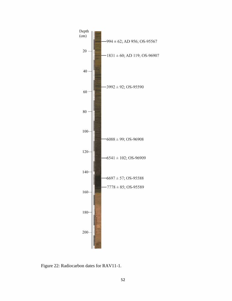
52
Figure 22: Radiocarbon dates for RAV11-1.

53
Fig
ure
23:
Dat
a fo
r R
AV
11
-1, th
e m
aste
r co
re f
or
Rav
en L
ake.
A
ges
wer
e ca
lcula
ted w
ith t
he
age
model
. Y
-axis
tic
k m
arks
rela
te t
o
dep
th. T
he
blu
e li
ne
indic
ates
a c
ore
bre
ak b
etw
een R
AV
11
-1A
-1 a
nd R
AV
11
-1A
-2. T
he
firs
t gra
in s
ize
pan
el s
how
s d
ata
mea
sure
d o
n
a C
oult
er C
ounte
r, w
her
eas
that
in t
he
stra
tigra
phic
colu
mn w
as b
ased
on v
isual
obse
rvat
ion. T
he
firs
t gra
in s
ize
pan
el i
s se
par
ated
into
per
cent
clay
(blu
e), si
lt (
gre
en),
and s
and (
red).
The
stra
tigra
phic
colu
mn w
idth
is
det
erm
ined
by g
rain
siz
e cl
ay (
c), si
lt (
Si)
, sa
nd (
S),
and p
ebble
(P
). G
reen
po
ints
indic
ate
loca
tion o
f ra
dio
carb
on s
ample
s.

54
Sediments show only minor fluctuations in MS around a mean of 4x10⁻⁵
SI. The
highest values (~9x10⁻⁵
SI) occur between 38 and 35 cm depth, corresponding to a
massive band of silt. The percent organic material also shows only minor variations
around a mean of ~27%. A slight peak occurs around 90 cm depth. In contrast, percent
carbonate decreases up core in two steps at 40 and 120 cm depth. The blue scale, similar
to the MS and organic content, fluctuates only slightly.
Despite the abundance of organic material in the sediments, I did not find any
macrofossils. Therefore, I selected radiocarbon samples to be spaced evenly throughout
the core (Table 2). Five AMS samples dated were from 125.5 cm (OS-96909, 6541 ± 102
cal. yBP), 111 cm (OS-96908, 6088 ± 99 cal. yBP), 56 cm (OS-95590, 3992 ± 92 cal.
yBP), 24 cm (OS-96907, 1831± 60 cal. yBP), and 9 cm depth (OS-95567, 994 ± 62 cal.
yBP).
3.2.3.2 RAV11-1A-2
RAV11-1A-2 (Fig. 22, 23) is the second thrust in the same hole, and therefore the
core should be a continuation of RAV11-1A-1.
Basal clay coarsens upward into silt and sand from 73-58 cm depth. Pebbles are
present below 66 cm depth. This unit grades into a pink and gray (5YR 5/1) sand that
extends to 29 cm depth. This sand has distinct medium-grained sand and pebble bands
intermixed with fine sand layers. The sand unit grades into a massive pink and gray (5YR
5/1) silt, which occurs from 18-29 cm depth. Finely laminated (millimeter-scale) silt
overlies this silt with a sharp contact at 18 cm depth. Laminae combine to form
alternating centimeter-thick bands of dark grayish-brown (2.5Y 4/2), olive brown (2.5Y
55
4/4), and black sediment. From 15-18 cm depth, the silt is a massive dark grayish-brown
(2.5Y 4/2).
MS data are variable and range as high 55x10-5
SI. The organic and carbonate
content are negligible. At the contact with the organic silt at 18 cm depth, the organic
material increases to ~25%, which it maintains through the upper part of the core.
Carbonate increases ~11%.. Color intensity follows the same pattern as other proxies.
I found only limited macrofossils in the laminated organic silt and therefore had
to sieve samples to concentrate the organic remains present. I sent two samples for
analysis (Table 2). Sample OS-95588 (4 cm depth) yielded an age of 6697± 57 cal. yBP,
and sample OS-95589 (11 cm depth) provided an age of 7778 ± 85 cal. yBP
3.2.3.3 RAV11-2A-1
RAV11-2A-1 (Fig. 24, 25) is composed of a finely laminated (millimeter-scale)
silt. The fine laminations group together to form larger color bands (centimeter scale),
alternating between olive brown (2.5Y 4/4) and black. A change in color occurs at 82 cm
depth, and the core alternates between very dark brown (2.5 Y 3/1) and black. This
sediment type persists throughout the core except for prominent light tan layers (0.1-0.5
cm thick) at 29 and 56 cm depth.
The MS and color intensity vary around a mean of ~2x10⁻⁵
SI and 70,
respectively, throughout the core. The MS has a large, sharp, short peak of ~42x10-5
SI at
67 cm depth. A smaller corresponding peak also occurs in the color profile. I did not
identify any change in sediment type at this depth.

56
Figure 24: Radiocarbon dates for RAV11-2A-1.

57
Fig
ure
25:
Dat
a fo
r R
AV
11
-2A
-1. Y
-axis
tic
k m
arks
rela
te t
o d
epth
. T
he
firs
t gra
in s
ize
pan
el s
how
s dat
a m
easu
red o
n a
Co
ult
er
Counte
r, w
her
eas
that
in t
he
stra
tigra
phic
colu
mn w
as b
ased
on v
isual
obse
rvat
ion. T
he
firs
t gra
in s
ize
pan
el i
s se
par
ated
into
per
cent
clay
(blu
e), si
lt (
gre
en),
and s
and (
red).
The
stra
tigra
phic
colu
mn w
idth
is
det
erm
ined
by g
rain
siz
e cl
ay (
c), si
lt (
Si)
, sa
nd
(S),
and p
ebble
(P
). G
reen
poin
ts i
ndic
ate
loca
tion o
f ra
dio
carb
on s
ample
s.

58
I sent two samples for AMS radiocarbon dating (Table 2). Sample OS-95566 (14
cm depth) yielded an age of 6022 ± 102 cal. yBP. The second sample (OS-95569, 76 cm
depth) dated to 9145 ± 132 cal. yBP.
3.2.3.4 RAV11-3A-1
The lowest 58 cm of RAV11-3A-1 is composed of poorly-sorted , pink-gray
(5YR 5/1) medium-grained sand (Fig. 26, 27). From 17-25 cm depth, the sand becomes
finer and alternates with multiple bands of clay at 17-19 cm depth. At 17 cm depth, the
sediment changes abruptly to a finely laminated (millimeter-scale) silt that persists to the
top of the core. The laminae are grouped together to form larger, dark olive gray (5Y 3/2)
and black bands (centimeter-scale).
MS values vary significantly in the sand, ranging from ~0-38 x10-5
SI and drop
abruptly at 17 cm depth to ~6 x10⁻⁵
in the silt. Color intensity shows a similar pattern
being highest in the sand (~125) and decreasing abruptly at the contact with the overlying
silt.
A radiocarbon sample (OS-100776, table 2) directly at contact between the sand
and laminated silt (17 cm depth) dated to 12,525 ± 96 cal. yBP.

59
Figure 26: Radiocarbon dates for RAV11-3A-1.

60
FF
igure
27:
Dat
a fo
r R
AV
11
-3A
-1. Y
-axis
tic
k m
arks
rela
te t
o d
epth
. T
he
firs
t gra
in s
ize
pan
el s
ho
ws
dat
a m
easu
red o
n a
Coult
er
Counte
r, w
her
eas
that
in t
he
stra
tigra
phic
colu
mn w
as b
ased
on v
isual
obse
rvat
ion. T
he
firs
t gra
in s
ize
pan
el i
s se
par
ated
into
per
cent
clay
(blu
e), si
lt (
gre
en),
and s
and (
red
). T
he
stra
tigra
phic
colu
mn w
idth
is
det
erm
ined
by g
rain
siz
e cl
ay (
c), si
lt (
Si)
, sa
nd (
S),
and
peb
ble
(P
). G
reen
poin
ts i
ndic
ate
loca
tion o
f ra
dio
carb
on s
ample
s.

61
CHAPTER 4
DISCUSSION
4.1 Age Model
4.1.1 Radiocarbon Date Quality
Thirty-nine samples were dated for this study, and only two (OS-96948, OS-
100382) yielded ages inconsistent with their stratigraphic position. The measured δ13
C
for the radiocarbon samples are similar to accepted values for lake algae (Meyers and
Lallier-Vergès, 1999).
There is no evidence for a significant reservoir effect in the studied lakes.
Bedrock surrounding the lakes lacks carbonate material. Moreover, water entering Bunny
and Rapids Lakes flowed over bedrock for a large distance and with a great deal of
turbulence, causing aeration of the water. Rapid and Bunny Lakes, in particular, should
be well-mixed, because of the through-flowing current. All lakes recorded summer
temperatures above 4°C. As the surface water cools to 4°C during the winter freeze up it
will sink to the bottom of the lake, mixing the water and preventing long residence times.
Finally, Lusas (2011) obtained a modern age for lacustrine algae at the sediment-water
interface in a very similar lake farther east in the Scoresby Sund region. For all of these
reasons, I do not anticipate any significant reservoir effect either from input of old carbon
or long water residence times.

62
4.1.2 Rapids Lake
The age model for the Rapids Lake master core is based on five radiocarbon dates
(Table 4, Fig. 28). Sample OS-96048, at 10 cm depth, produced an age significantly older
than the next two lower dates and thus may contain reworked organic material washed in
from the land. Because it is out of stratigraphic order, and because it appears anomalous
old for such a shallow depth, I consider it to be in error. Therefore, for the rest of the
discussion I ignore OS-96048.
Ideally, the age model would take into account different deposition rates
documented by significant changes in sediment type. However, due to the lack of
radiocarbon dates below 38 cm depth, the age model for the lower 70 cm of the master
core was based on the best fit between samples OS-96045 and OS-95933 and is thus only
a first-order approximation of age. I also set the top of the sediments at -60 cal. yBP
(using the convention that year 0 is AD 1950), since it appeared that we collected the
sediment-water interface.
4.1.3 BNL11-1
The master core for southern Bunny Lake, BNL11-1, was constructed from
BN11-1A-1 and BNL11-1B-1 (Table 4, Fig. 29). Based on stratigraphic correlation, I
matched the three gray bands that punctuate the organic-rich silt in both cores tying 107
cm depth in BNL11-1A-1 with 87 cm depth in BNL11-1B-1. Radiocarbon dates (OS-
95587, OS-95586) confirm the overlap at this depth within error of the ages.
Six radiocarbon dates provide the basis for the age model in the upper 120 cm of
the master core. Below 120 cm depth, I did not find any organic material, so the age of

63
this section is unconstrained. Several thin (0.1 cm thick) gray bands punctuate the
organic-rich silt from 98-120 cm depth, a characteristic not observed in the organic-rich
silt higher in the core. Therefore, I fit two separate lines between the radiocarbon ages in
both units to provide a sedimentation rate.
4.1.4 BNL11-2
BNL11-2, the master core for the northern basin of Bunny Lake, is constructed
from BNL11-2A-1 and BNL11-2A-2, the second thrust in the same hole (Table 4, Fig.
30). I used eighteen dates to produce the age model. OS-100382 (3430 ± 30 cal. yBP) is
anonymously young for its depth compared to the surrounding radiocarbon dates. Even
with the two sigma range of the calibrated radiocarbon date, OS-100382 differs from both
the age model and the surrounding radiocarbon dates. Therefore the radiocarbon date is
significantly young and out of stratigraphic position. For the remainder of the paper I
ignore this sample. Other dates, such as OS-100378 and OS-100379, are not in proper
sequence, but are within error of each other so the difference is not significant.
I divided the core into three segments composed predominantly of non-glacial
organic-rich silt to account for variations in the sedimentation rate that may have
occurred during the Holocene. Breaks between segments occurred at large, grey,
inorganic layers. Within each segment, I fit a line through the radiocarbon dates to
produce the age model.

64
Figure 28: RPD11-1 age model. Red squares show radiocarbon dates. Light blue
diamonds are out of stratigraphic order and are omitted.
Figure 29: BNL11-1 age model. Red squares show radiocarbon dates.

65
4.1.5 Raven Lake
I constructed the master core, RAV11-1, from RAV11-1A-1 and RAV11-1A-2
(Table 4, Fig. 31). There was no organic matter below 160 cm depth, so the age of the
deepest sediments is unknown. Above 160 cm depth, the core is very finely laminated
gyttja, and the sedimentation rate appears to be relatively constant. I fit a line through all
seven radiocarbon dates to provide control for the age model.
Table 4: Age model for master cores.

66
Figure 30: BNL11-2 age model. Red squares show radiocarbon dates. Light blue
diamonds are out of stratigraphic order and are omitted.
Figure 31: RAV11-1 age model. Red squares show radiocarbon dates.

67
4.2. Lake History
4.2.1 Raven Lake
The lowest sediments in the Raven Lake cores, coarse sand and gravel commonly
set in a clay matrix, likely represent ice-proximal conditions during deglaciation of the
area. From 160-210 cm depth, RAV11-1 is characterized by interbedded sand and gravel
which show oscillations between finer and coarser sediment. These changes in grain size
may represent variations in the glacier, with the larger sediment representing times when
the margin was closer to the lake. They also could represent differences in the type of
sediment deposited from an adjacent ice margin. Due to the lack of dating constraints, I
am unable to identify the time scale of these fluctuations.
Laminated gyttja overlies the sand and gravel. A radiocarbon date from RAV11-
3A-1 at the contact with the sand, provides a minimum-limiting age for onset of organic
sedimentation and for deglaciation of the lake of 12,614 ± 89 cal. yBP (OS-100776). A
second radiocarbon date from RAV11-1A-2, taken eight centimeters above the same
transition dates to 7778 ± 85 cal. yBP (OS-95589). A sample from RAV11-2A-1 at a
lower depth than the contact from sand to gyttja in RAV11-1 yielded an age of 9145 ±
132 cal. yBP (OS-95569). RAV11-2 does not contain the deglacial-gyttja contact, so I am
unsure how closely this age constrains the transition, However, this date is at least
broadly consistent with the old age for deglaciation obtained from RAV11-3A-1.
The depth of the sand/gyttja contact differs among cores and indicates that the
sand surface has topography. In RAV11-1A-2, the transition from sand to silt occurs at
~1720 cm below lake surface level, but in RAV11-3A-1 it occurs at 1770 cm depth. The
silt continues to depths greater than 1770 cm in RAV11-2A-1, so the contact must be

68
even lower. During deposition, the coarse sediments either were not laid down as a flat
surface, or subsequent erosion created an irregular topography. When the gyttja was
deposited in the lake, it ponded in the deeper sections first. However, additional
radiocarbon samples need to be dated from the contact to help support this claim.
Very finely laminated silts occur throughout the rest of the core. Although one
cannot be certain, it is possible that these laminae are varves. The lowest 50 cm of the
laminated organic silt is coarser than the top 110 cm. A gradual transition to the smaller
grain size is centered at ~110 cm depth at ~5800 cal. yBP. and may represent a mid-late
Holocene change in climate. Before grain size was measured, I removed organic material
and biogenic silica which make up a large fraction of Raven Lake sediments. Therefore,
the measured grain size represents inorganic material washed or blown into the lake. The
increase in grain size could represent a mid-Holocene increase in local runoff from
precipitation or snowpack melt, or an increase in wind.
Conditions were relatively stable from ~5800 cal. yBP to present at Raven Lake.
Although the MS does not show any significant changes, the percent of organic material
decreases above ~80 cm depth and carbonate throughout the core from 12% at the base to
near 1%. This carbonate may be associated with algae blooms (Stabel, 1986). If so, the
decrease in carbonate and organic material may represent a change in the lake ecosystem
over time.
The lack of any obvious glacial input in this lake constrains the size of the
Renland Ice Cap over the Holocene to within ~200 m of the present-day margin. The
abandoned channel that enters the northeast end of the lake heads just distal to the LIA
drift edge about 200 m from the current glacial margin. The glacier could not have

69
advanced past the stream head or silt-laden meltwater would have entered Raven Lake.
Such sediment is absent from the lake after initial deglaciation in late-glacial time. Thus,
I infer meltwater produced by the glacier during the LIA and during other expansions of
similar or smaller size would have by-passed Raven Lake and drained through the
prominent meltwater channel that extends from the present-day glacial margin to Large
Lake.
The purpose of a control lake, such as Raven Lake, is to highlight evidence of
non-glacial events, such as storms or landscape erosion, that can be interpreted
mistakenly as being of glacial origin. In Raven Lake, there is no evidence, such as bands
of inorganic silt or sand, of any event disrupting normal sedimentation. Therefore, it is
likely that the significant changes in sedimentation observed in the nearby glacially fed
lakes are the result of glacial activity and not other factors.
4.2.2 Rapids Lake
The lowest radiocarbon date in Rapids Lake cores affords a minimum age for
deglaciation of 8115 ± 103 cal. yBP (OS-95933) and comes from interbedded silt and
fine sand that overlies coarser sand lost during retrieval. I interpret the variation between
laminated black silt, coarser reddish gray silt, and reddish gray fine sand from 84-108 cm
depth as representing glacial meltwater variations across a threshold. Glacial material
(reddish-gray silt and sand) entered the lake from 8100-8800 (99-106 cm depth), 7700-
7800 (95-96 cm depth), 7300 (91-92 cm depth), 7100 (89.5 cm depth), and 6600 cal. yBP
(84 cm depth) In contrast, the black, organic-rich, laminated silt is characteristic of a lake

70
with limited glacial input and may represent periods when Rapids Lake no longer
received meltwater.
The reddish-gray sand and silt differ from other inorganic layers in Rapids Lake
in color and MS values. In addition, the sand grades into the silt, a relationship not seen
higher in the core. This gradation could reflect recession of ice in the basin and
increasing distance of the glacier from the lake. Moreover, based on color, this silt and
sand may have a different source from the inorganic gray bands in the core. One
possibility is that the glaciers were more expanded early in the lake history than at any
time since and were depositing sediments derived from areas that later remained
unglaciated.
The reddish-gray sand and silt also could be deposited in different ways, such as
from a mass movement into the lake. However, this explanation is unsatisfactory,
because the maximum grain size is very fine sand. If a mass movement occurred, the
resulting deposit might be less well sorted and potentially include larger sediments, given
the large grain sizes available around the lake shore. Another possibility is that they could
represent inwash from runoff during a large storm event. However, the absence of similar
inorganic bands in Raven Lake is circumstantial evidence against this hypothesis. A third
explanation is that wind or mass movements deposited sediment onto an ice-covered lake
during the winter that later melted through during spring break up, but again a poorly
sorted deposit would be expected. Yet another possibility is that channels, heading on the
adjacent plateaus, collect aeolian sand and silt when not draining water. Once the
channels become reactivated by meltwater, the sediments may be washed out into the
lake during the initial flushing, creating sand layers that grade into glacial silt. Although

71
many of these explanations are possible, the simplest is that the reddish-gray sand and silt
bands resulted from glacial meltwater and material entering the lake, particularly as their
stratigraphic position suggests that they formed soon after the lake itself was deglaciated.
At 84-86 cm depth (6500-6800 cal. yBP), there is an abrupt, large decrease in
organic content that corresponds to a thick gray band in the stratigraphy. This likely
represents a glacial advance. After this event, the organic material increases to higher
levels which are maintained to about 40 cm depth (~1900 cal. yBP). I interpret this
organic unit to represent that the lake was receiving minimal or no glacial sediment with
the exception of brief periods described below. Today, Rapids Lake receives rock flour
and deposition is largely inorganic. This comparison suggests that overall, the mid-
Holocene was a period with glaciers and meltwater discharges that were smaller than at
present. However, there are several prominent gray clayey-silt bands that interrupt the
brown organic silt. Based on the age model, prominent layers formed at ~5900 (77 cm
depth), 5100 (70.5cm depth), 4800 (66 cm depth), and ~3400 (52.5 cm depth) cal. yBP.
Multiple bands were deposited between ~2300 and 3600 cal. yBP (42-55 cm depth). This
presence of inorganic, more clay-rich, gray sediments, likely reflects periods of enhanced
glacial meltwater influx to the lake, and therefore glacial expansion.
From ~38 cm depth to the surface, the sediments consist primarily of a thick layer
of inorganic, gray clay typical of glacial rock flour interbedded with dark brown clayey-
silt laminae at 22-23, 15-18, 14-15, and 5-8 cm depth. The clay unit is much thicker than
any of the gray bands seen lower in the core, suggesting it represents the largest glacial
advance recorded since the initial deglaciation of Rapids Lake. This clay is constrained
with a maximum-limiting radiocarbon date of 1940 cal. yBP (OS-96045), which was

72
taken from two centimeters below the contact. However, due to the slow sedimentation
rate of the organic silt, this age could be significantly older than the onset of glacial
sedimentation, which is constrained only to less than ~1900 cal. yBP. Since the clay unit
continues to the top of the core, it contains the time period of the LIA, but it also may
include earlier glacial fluctuations.
The gray clay contains minor layers of massive dark brown silt, two of which are
capped by orange oxidized layers at 22 (322 cal. yBP, AD 1620) and 15 cm depth (135
cal. yBP, AD 1815). These bands represent a change in the oxidation state at the lake
bottom. Such changes can come about by lowering of water level. However, it seems odd
that lake level would drop during what is generally thought to be a period of expanded
glaciers. Water level is controlled by a bedrock outlet, so a drop in lake level would
require a significant reduction in water input – likely cessation of outflow from Large
Lake.
Overflow from Large Lake could have been stopped if the ice dam was breached
(or floated) and water drained northeast catastrophically. Water would return to Rapids
and Bunny Lakes when the dam reformed. . An alternative is that the layers may
represent oxidized material washed into the lake. However, reworking of material would
likely produce a poorly sorted, non-uniform deposit. More study of these layers is
necessary before their origin can be understood fully.
Unlike silt deeper in the core, the dark brown silt laminae that interrupt the clay
are not of organic origin. One possibility is that during the advance represented by the
clay, the largest in the last 8000 cal. yBP in Rapids Lake, plateau glaciers above the lake

73
may have reformed, allowing contribution of local, and thus more coarse, glacial material
to the lake during the coldest intervals.
Sedimentation in Rapids Lake at present does not differ significantly from that
during the LIA. The lake is still receiving glacial flour from Large Lake, and organic
growth has not returned to values present before the deposition of the clay.
4.2.3 Bunny Lake
Poorly sorted sand and gravel that are typical of proximal glacial deposition
comprise the lowest 33 cm of BNL11-1. Larger pebbles (as much as five centimeters in
diameter) were probably ice-rafted debris. If so, this would require that ice occupied part
of either Rapids or Bunny Lake in order for icebergs to reach the core site.
The timing of deglaciation is constrained by minimum-limiting radiocarbon dates.
Sample OS-95640 is from an algae mat directly at the abrupt contact between the poorly-
sorted sand and gravel and the overlying laminated organic-rich silt in the southern basin.
It yielded a minimum-limiting date of 7994 ± 67 cal. yBP for deglaciation. However, the
oldest radiocarbon date in the northern basin, OS-100779, affords a minimum-limiting
deglaciation date of 9494 ± 51 cal. yBP. Although this date is not directly at the contact
between the poorly-sorted sand and gravel and the overlying laminated organic-rich silt,
ice must have been absent from the northern (and probably both) basin by 9500 cal. yBP
to allow the deposition of the organic material. The difference in ages between the two
basins is likely due to the oldest organic material not being deposited where BNL11-1
was collected, or to the current flowing over BNL11-1 creating an unconformity by
eroding material.

74
Directly above the basal sand and gravel, multiple gray laminae formed within
organic silt between ~9.5 and 7.4 ka. Similar to Rapids Lake, these laminations likely
represent oscillations in meltwater input. This may because either the glacier itself was
situated near a threshold or water level in Large Lake only periodically overflowed
through the western outlet.
Most sediment in BNL11-1 and BNL11-2 is composed predominantly of an
organic-rich silt which is black at the base of the unit and gradually lightens in color to a
dark grayish-brown. In BNL11-1, the organic silt began at ~8000 cal. yBP (119 cm
depth) and persisted to ~1050 cal. yBP (28 cm depth). In BNL11-2, the silt was deposited
from ~9500 cal. yBP (152 cm depth) to ~1340 cal. yBP (18 cm depth). In both cores,
organic material decreases slightly over time, possibly because of either a greater
contribution of glacial material in the second half of the Holocene or a decline in lake
productivity due to cooling climate or loss of nutrients.
In both cores, gray bands with increased MS and low organic content typical of
glacial sediment punctuate the organic silt. Gray sediments were deposited in BNL11-1 at
~7200-7400 (98-100 cm depth), 6400 (86 cm depth), and ~3000 cal. yBP (52 cm depth).
The gray bands are more pronounced and numerous in core BNL11-2 (Table 5). Those at
~8700, ~7400, and ~6000 cal. yBP have fine sand, similar to that seen at the base of
Rapids Lake, which grades into gray clay. The lowest gray band, at 152-156 cm depth,
ended at 9494 ± 51 cal. yBP and may reflect the onset of organic sedimentation following
deglaciation of the lake. These gray bands, represent events of significant size and
duration, in which glacial material swamped organic deposition in Bunny Lake.

75
Tab
le 5
: T
imin
g o
f gla
cial
advan
ces
of
the
Ren
lan
d I
ce C
ap. T
he
tim
e bet
wee
n e
ven
ts w
as c
alcu
late
d b
y f
indin
g t
he
amount
of
tim
e
bet
wee
n m
id-p
oin
ts. G
laci
al a
dvan
ces
occ
urr
ing o
ver
a s
hort
tim
e sp
an w
ere
gro
uped
toget
her
wit
h t
he
assu
mpti
on t
hat
thes
e m
ult
iple
even
ts r
efle
cted
an o
scil
lati
on w
ithin
a g
ener
al c
old
per
iod.
0p
rese
nt-6
0**
**
**
***
***
***
18
OS
-10
03
76
13
37
± 3
8
18
OS
-10
03
76
13
37
± 3
8**
**
**
***
***
***
19
OS
-10
03
77
13
46
± 3
9
--
-0
pre
sent
-60
0p
rese
nt-6
0
--
-26
OS
-96
87
41
062
± 8
538
OS
-96
04
51
940
± 5
3
51
OS
-10
03
78
36
42
± 8
653
OS
-96
90
63
023
± 6
152.5
Age
Mo
del
3400
61
OS
-10
03
79
35
11
± 6
80
.5 c
m thi
ck0
.2 c
m thi
ck
64
OS
-10
03
80
39
97
± 9
1
--
--
--
65
OS
-10
03
81
37
62
± 7
6
--
--
--
76
Age
Mo
del
4900
--
-66, 69.5
Age
Mo
del
4770,
77
OS
-10
05
16
49
60
± 9
4
--
-0
.1 c
m thi
ck5100
87
OS
-10
05
17
59
78
± 5
3
86
Age
Mo
del
6370
77
Age
Mo
del
5880
89
Age
Mo
del
6090
0.2
cm
thi
ck0
.3 c
m thi
ck
3 4 5 6 71
BN
L1
1-1
RP
D1
1
2
BN
L1
1-2
Rad
ioca
rbo
n
Sam
ple
Age
(ca
l.
yBP
)
Dep
th
(cm
)
Rad
ioca
rbo
n
Sam
ple
Age
(ca
l.
yBP
)
Gre
y
Ban
d
Dep
th
(cm
)
Rad
ioca
rbo
n
Sam
ple
Age
(ca
l.
yBP
)
Dep
th
(cm
)
Tim
ing
Tim
e
Sp
an
(ka)
5.8
-6.0
1.3
1.0
3.0
-3.6
3.7
-4.0
4.7
-5.0
Gla
cial
Ad
vanc
e (k
a)
1.1
****
****
2.6
1.2
1.4

76
Tab
le 5
: C
onti
nued
99
Ag
e M
od
el
7010
--
-84
Ag
e M
od
el
6590
0.3
cm
th
ick
--
-86.0
0A
ge M
od
el
6790
103
Ag
e M
od
el
7330
--
-89.5
Ag
e M
od
el
7140
0.1
cm
th
ick
--
-0.4
cm
th
ick
105
OS
-100777
7459 ±
46
98
OS
-95587
7298 ±
40
91
Ag
e M
od
el
7290
OS
-95586
7237 ±
80
122
OS
-100518
7370 ±
58
100
Ag
e M
od
el
7390
92
Ag
e M
od
el
7340
129
OS
-100519
7589 ±
33
--
-95
Ag
e M
od
el
7700
0.2
cm
th
ick
--
-96
Ag
e M
od
el
7800
134
OS
-100520
8101 ±
76
117
Ag
e M
od
el
7990
99
OS
-95933
8115 ±
103
141
OS
-100521
8323 ±
48
0.2
cm
th
ick
106
Ag
e M
od
el
8800
145
OS
-100778
8841 ±
150
--
--
--
148
OS
-100522
8678 ±
100
--
--
--
152
OS
-100779
9494 ±
51
--
--
--
**
*-
--
--
-
*E
nd
of
ev
en
t n
ot
cap
ture
d in
co
reP
eri
od
icit
y1.1
6
**
Ev
en
t 3 c
on
tin
uo
us t
o p
resen
t
**
*U
nab
le t
o d
iffe
ren
tiate
betw
een
fir
st
3 g
rey
ban
ds
**
**
Lik
ely
rep
resen
ts o
scilla
tio
ns w
ith
in a
co
ld c
lim
ate
BN
L11-1
RP
D11
Tim
ing
Gre
y
Ban
d
Dep
th
(cm
)
Rad
iocarb
on
Sam
ple
Ag
e (
cal.
yB
P)
Dep
th
(cm
)
Rad
iocarb
on
Sam
ple
Ag
e (
cal.
yB
P)
Dep
th
(cm
)
Rad
iocarb
on
Sam
ple
Ag
e (
cal.
yB
P)
Gla
cia
l A
dv
an
ce
(ka)
Tim
e S
pan
(ka)
BN
L11-2
9.4
8.1
-8.3
8.6
-8.8
1.2
0.9
**
**
**
**
7.0
-7.5
7.6
-7.8
13
1498 10
11
12

77
The number of glacial advances recorded in the two basins of Bunny Lake differs.
BNL11-2, taken from the northern basin, is in a low-energy environment removed from
the stream current. The lack of a strong current in the northern basin allows finer particles
to settle out and be deposited more readily than in the southern basin. Therefore, the
northern basin produced a higher-resolution, more sensitive record. The combined record
shows that the gray bands formed in both Bunny Lake basins at ~7200-7500, 6000-6300,
and 3000-3500 cal. yBP. Additional layers were deposited in BNL11-2 at 9400, 8600-
8800, 8200-8300, 7000, 4900, and 3700-4000 cal. yBP.
Gray clay produced by glacial sedimentation dominates the upper part of both
Bunny Lake cores. In BNL11-2, late Holocene clay deposition begins at ~AD 615 and is
constrained by two radiocarbon dates directly at the contact. In contrast, in BNL11-1 a
date in similar stratigraphic position constrains the start of clay deposition to shortly after
~AD 900. The AD 600 event is not seen, possibly because of erosion from the stream
current. Regardless, the upper unit is by far the largest magnitude glacial event in either
core. If thickness of sediments is a measure of glacier size and duration, the glacial
expansion that caused this upper clay unit was the largest in the Holocene.
The upper clay unit is not uniform. In both basins, it is punctuated by massive fine
sand similar to that seen in some of the lower gray bands and not far different from the
coarse silt layers that occur within the clay in Rapids Lake. In BNL11-1, sand input
began at AD 1470, as dated by a radiocarbon sample taken at the base of the layer. In
BNL11-2, a date from the middle of the sand layer indicates that it was still being
deposited at AD 1644. Since the younger date was taken from the middle of the layer and
the older from the base, it appears that the sand was deposited over time and not in a

78
single pulse. If true, this rules out flushing of an abandoned channel, mass movement,
melting through lake ice, or storm in wash events as possible causes for the sand. One
possibility is that meltwater from glaciers on the plateaus above the lake could transport
coarse sediment into Bunny Lake. If this were the case, then the length of the time that
the sand was deposited reflects the presence of glacial ice on the plateau. Similar to
Rapids Lake, the upper gray clay is punctuated further in both cores by multiple 0.1 cm-
thick bands of bright orange oxidized material, which may reflect brief intervals of lower
lake level.
Bunny Lake is currently still receiving meltwater and rock flour from Large Lake,
and the MS, percent organic material and carbonate are similar to that seen during the
LIA. We would expect the lake to show glacial conditions until either meltwater into
Large Lake decreases or the ice dam is removed, allowing draining to the northeast.
Based on comparison with lower sediments in the cores, the configuration of the Renland
Ice Cap has not yet returned to what it was prior to ~AD 600, when little to no glacial
sediment entered Bunny Lake.
4.3 Glacial History of Raven, Rapids, Bunny Lake
If the basal age in RAV11-3A-1 is correct, then the Renland Ice Cap retreated
from Raven Lake by ~12.6 ka, possibly at the end of the Milne Land Stade (Hall et al.,
2008a). Raven Lake lies just inboard of degraded moraines that, based on position and
weathering, could date from the Milne Land Stade. Moreover, the lake shows evidence of
a higher past level, possible only if ice significantly more extensive than it is now
dammed existing outlets. This is consistent with the lake being deglaciated soon after the

79
Milne Land Stade but while extensive ice was still present in valley occupied now by
Large Lake. The end of the Milne Land Stade in central Scoresby Sund may have taken
place before ~12.5 ka (Hall et al., 2008b) based on a relative sea-level curve for nearby
Kjove Land. Such an early glacial retreat was not observed in Bunny and Rapids Lake,
which instead provide minimum-limiting ages for deglaciation of 9.5 ka. I cannot be sure
if this difference in basal ages between the sites reflects a time difference in deglaciation
or simply the fact that we did not retrieve the lowest sediments from Bunny and Raven
Lakes. Moreover, additional work is needed to confirm the early age for deglaciation at
Raven Lake.
At Raven Lake, organic deposition persisted for the entire Holocene without any
obvious interruption by glacial sediment. Based on evidence given above, I infer that the
Renland Ice Cap was not more extensive that it was during the LIA at any time during the
Holocene. This limits ice extent to within ~200 m of its present margin. It also suggests
rapid retreat after deglaciation in late-glacial time to or within present-day ice-cap limits.
Organic-rich silt also was deposited in Rapids and Bunny Lakes. The basins have
the highest organic content in the early- to mid-Holocene, indicating it to be the time of
the most productive lakes or the least glacial input. Additional lacustrine records from the
Arctic, based on biogenic silica (e.g. Wagner et al., 2000; Cremer et al., 2001; Pordriske
and Gajewski, 2007; McKay and Kaufman et al., 2009) show high lake productivity at
approximately the same time (7-5 ka). This period of enhanced productivity is
traditionally linked to the Holocene Thermal Maximum (9-5 ka) (Larsen et al., 1995).
After the early to mid-Holocene, cores in all three lakes lighten in color, blue
color intensity increases, and percent organic material lowers slightly. This gradual

80
decrease of organic material occurs throughout the cores until the final late Holocene
glacial advance when organic content drops to near zero. The gradual decline of organic
material over the late-Holocene may indicate an increasing contribution of silt-laden
meltwater from the glaciers diluting the organic percent, or a decrease in production of
organic material in the lake due to climate or nutrient changes. The fact that the non-
glacial Raven Lake also shows a increase in blue color intensity and a small decline in
organic content and that there is a corresponding decrease in biogenic silica in lakes
across the Arctic (e.g. Wagner et al., 2000; Cremer et al., 2001; Pordriske and Gajewski,
2007; McKay and Kaufman et al., 2009) argues for a change in productivity.
Both glacially fed lakes have short periods of significant glacial input
superimposed on the overall record. Based on the presence of inorganic gray clay layers
inferred to be rock flour, glaciers were expanded at 9.4, 8.6-8.8, 8.1-8.3, 7.6-7.8, 7.0-7.5,
5.8-6.0, 4.7-5.0, 3.7-4.0, and 3.0-3.6 ka. (Table 5). In addition, glacially fed lakes show a
large late Holocene event at or after ~1.4 ka, culminating in the LIA. With the exception
of the LIA, most events appear to be of short duration and radiocarbon dates constraining
the beginning and end of each event commonly overlap. To test whether these events
were periodic, I calculated the time interval between clay layers (Table 5) and then
averaged the time spans. I grouped events that occurred close together into a single event
and compared the interval between mid-points. There is a rough cyclicity of 1160 years. I
assume the 2300-year gap between events in the early Holocene represents a double
event. Therefore I calculated the periodicity only with the other values. The variation of
times between glacial advances may indicate that the cycle is weak or that the cores do
not record every event.

81
4.4 Comparison of Climate Records
4.4.1 Comparisons between the Renland Glacial Record and the Renland Ice Core
Renland is important, because it is one of only a few sites that allow direct
comparison of glacial-margin fluctuations and an ice-core record reconstructed from the
same ice mass. Differences between climate proxies can give information on climate and
forcing mechanisms. For examples, offsets between temperatures reconstructed from
both glacier snowlines and ice-core proxies can indicate changes in seasonality (e.g.,
Denton et al., 2005), because snowlines record summer conditions and ice cores mean
annual.
The Renland Ice Cap was cored to bedrock (Johnsen et al., 1992). Although
earlier studies did not find any significant centennial-scale climate events, such as the 8.2
ka event (Johnsen et al., 1992), a new time scale (Fisher et al., 1996), as well as
reanalysis at higher resolution (Vinther et al., 2008), resulted in an improved record. The
new δ18
O record shows a warm early Holocene, peaking around 9 ka. The δ18
O values
then are interpreted as showing a steady decline in temperatures over the rest of the
Holocene. Short-term, abrupt climate cooling occurred at 9.3 and 8.2 ka (Fig. 32).
Broadly, the glacial margin and ice-core records from Renland are in agreement
(Fig. 32). The ice core indicates sudden warming during deglaciation from the Milne
Land Stade from ~12.5-10 ka. Two abrupt cooling events at 9.3 and 8.2 ka may correlate
with glacial advances. All of the cores from glacially fed lakes show multiple fluctuations
in meltwater input through this time period. The presence of mostly non-glacial,
relatively high-organic content, lacustrine sediments in the early Holocene are consistent

82
Fig
ure
32:
Com
par
ison w
ith G
reen
land i
ce c
ore
s. (
A)
and (
B)
show
sola
r in
sola
tion c
urv
es f
or
Jun
e an
d D
ec.
for
60°
N t
hro
ughout
the
Holo
cene
(May
ewsk
i et
al.
, 2004).
(C
) T
ota
l so
lar
irra
dia
nce
sm
oo
thed
wit
h a
40 y
ear
aver
age
rela
tive t
o t
he
inte
nsi
ty i
n 1
986
const
ruct
ed f
rom
1⁰B
e io
ns
in t
he
GIS
P2 i
ce c
ore
(S
tein
hil
ber
et
al., 2
009).
(D
), (
E),
and (
F)
are
δ18
O p
rofi
les
for
NG
RIP
(V
inth
ter
et a
l., 2009
), D
YE
3 (
Vin
ther
et
al., 2
009)
and G
ISP
2 i
ce c
ore
s (G
roote
s a
nd S
tuiv
er, 1997).
(F
) G
ISP
2 s
sNa
conce
ntr
atio
n (
ppb)
thro
ughout
the
Holo
cene.
(O
’Bri
en e
t al
., 1
995).
(H
) P
aleo
tem
per
ature
rec
onst
ruct
ion o
ver
the
GIS
fro
m tr
apped
N a
nd A
r in
the
GIS
P2 i
ce c
ore
(K
obas
hi
et a
l., 2011).
(I)
δ18O
pro
file
s fo
r R
enla
nd i
ce c
ore
(V
inth
er e
t al
., 2
008)
(J)
Per
iods
of
gla
cial
expan
sion o
f
the
Ren
land I
ce C
ap d
eter
min
ed t
hro
ugh p
rogla
cial
lak
e se
dim
ents
. T
he
blu
e blo
cks
indic
ate
per
iods
of
gla
cial
exp
ansi
on
, an
d t
he
dott
ed b
ord
ers
show
adv
ance
s se
en o
nly
in B
NL
11
-2. T
he
ques
tion m
ark s
pec
ifie
s th
at t
he
low
er b
oundar
y o
f th
e gla
cial
adv
ance
is
unknow
n.

83

84
with a warm period of low glacial activity, which agrees well with the HTM from 9-5 ka
(Larsen et al., 1995) recorded in the ice core. However, the peak temperature in the ice
core occurred at ~9 ka (Vinther et al., 2008), something that is not obvious in the lake
records, which show fluctuating glacial activity from 8-9 ka. After the HTM, both the
decreasing organic content in the glacially fed lake sediments and the ice core δ18
O
records suggest a changing climate, possibly cooling conditions through the rest of the
Holocene.
The major difference between the records from the glacially fed lakes and the ice
core is that none of the small centennial-scale glacial advances shown in the lacustrine
sediments after 8.2 ka occur in the Renland ice core δ18
O data. This contrast is
demonstrated best by the LIA. The ice-core record does not show significant variation
during the event (Vinther et al., 2008). However, the local ice caps expanded to their
largest extent during the Holocene at this time (e.g., Hall et al., 2008a; Kelly et al., 2008;
Lusas, 2011; This study). The lack of high-frequency events in the ice core may be
related to the low sampling resolution. However this is unlikely because the 8.2 ka event
was observed in the core. The LIA was longer in duration, and since it is younger, less
thinning would have occurred to the ice. Therefore the LIA should be easier to detect
than the 8.2 ka event. A second possibility is that the δ18
O of the Renland is cap is not
recording a pure temperature signal. Instead the record may be influenced by moisture
source or precipitation height (Johnsen et al., 1992) Another option is that the mean
annual conditions, as recorded by ice cores, did not change significantly on millennial
timescales, while summer temperatures, documented by glacier extent, fluctuated.. If this
were the case, then winter temperatures would have had to have changed opposite that of

85
the summer in order to produce the same mean value. This would result from decreased
seasonality, with colder summers and warmer winters. In order to test this hypothesis
more fully, the Renland ice core needs to be analyzed at high resolution for other proxies,
including trapped gases that independently record temperature (i.e., Kobashi et al., 2011).
4.4.2 Holocene Glacier and Climate Fluctuations in Greenland
The results from my field area fit well with other glacier and climate
reconstructions in Greenland. Glaciers retreated to positions similar to or less extensive
than at present by the early Holocene and remained behind the LIA limit throughout the
HTM, the timing of which is dependent upon location (Kaufmann et al., 2004). In
Greenland, the Renland ice core (Larsen et al., 1995), pollen studies (e.g. Fredskild,
1984; Wagner and Melles, 2002; Cremer et al., 2001), and warm-water mollusks in raised
marine deposits (e.g. Hall et al., 2008a; Street,1977) indicate warm temperatures from
~9-5 ka. However, the HTM begins at ~11 ka in Alaska and northwest Canada and is not
recorded in the Hudson Bay region until ~7 ka. This spatial variability may be related to
the presence of remnants of the LIS, ocean currents, and different positive feedbacks in
the widely separated regions (Kaufmann et al., 2004). Our study agrees with Larsen et al.
(1995) who identified the HTM in the Renland ice core between 9-5ka.. Sites at lower-
elevation, coastal locations north of Scoresby Sund, Ymer Ø (Wagner and Melles, 2002)
and Geographical Society Ø (Cremer et al., 2001), reached maximum temperatures and
organic productivity at ~8 ka and ~8.5-7 ka, respectively.
The timing of the HTM maximum may be related to latitude and elevation. The
NGRIP and GRIP ice-core temperature records match well, except that the highest

86
Holocene temperature at NGRIP was reached a few centuries before that at GRIP
(Johnsen et al., 2001). Both of these show high temperatures from roughly ~8-4.5 ka,
whereas the Dye 3 record, at lower elevation in South Greenland, does not show the
HTM until 4.5-4 ka (Dahl-Jensen et al., 1998). This pattern suggests a possible north to
south progression of the HTM.
The timing of the HTM in Scoresby Sund may be partially the result of the
changing strength of the warm Irminger and the cold East Greenland Currents. The
Irminger Current carries saline- and nutrient-rich Atlantic water north. It splits just south
of the Denmark Strait, with one branch continuing to flow north and the other flowing
south around the southern tip of Greenland. In contrast, the East Greenland Current
carries relatively fresh water from the Arctic south along the eastern coast of Greenland.
Jennings et al. (2011), based on marine sediment proxies, argued that, particularly at 6.8-
4.5 ka, the Irminger Current flowed farther north than at present, bringing warm water up
the coast. They further proposed that the change in the current position was related to the
strength of the North Atlantic Oscillation (NAO). Warm-water mollusks in raised marine
deposits (e.g. Hall et al., 2008a; Street,1977) confirm warmer-than-present-ocean
conditions at this time in the Scoresby Sund region.
Porter and Denton (1967) defined Neoglaciation as the growth and
reestablishment of alpine glaciers after the HTM. The timing of this transition in East
Greenland is difficult to define precisely because elevation and geography play an
important role in glacial growth (Fig. 33). Because of the differences in elevation, the
response of glaciers within Scoresby Sund region to changes in forcing is not
synchronous. Bone Lake, a threshold lake of the Istorvet Ice Cap in low-elevation (305-

87
Fig
ure
33:
Com
par
ison o
f H
olo
cene
gla
cial
mar
gin
rec
ord
s fr
om
the
Nort
her
n H
emis
pher
e. (
A),
(B
), (
C),
(D
), (
E)
Per
iods
of
gla
cial
expan
sion
of
the
Ven
due
Gla
cier
(W
ilco
x, 2012)
Ren
land I
ce C
ap, Is
torv
et I
ce C
ap (
Lusa
s, 2
011),
Bre
gne
Ice
Cap
(L
evy e
t al
., i
n
revie
w)
and
a c
om
posi
te o
f nort
her
n h
emis
pher
e g
laci
ers
(Den
ton a
nd K
arlé
n, 1973).
The
blu
e box r
epre
sents
a p
erio
d o
f gla
cial
expan
sion
. T
he
x s
cale
is
unit
less
. T
he
dott
ed b
ord
ers
show
adv
ance
s se
en o
nly
in B
NL
11
-2 c
ore
. T
he
ques
tion m
ark
spec
ifie
s th
at
the
low
er b
oundar
y o
f th
e gla
cial
adv
ance
is
un
kn
ow
n. (
F)
Thin
bar
s re
pre
sent
the
life
span
of
a tr
ee i
n a
pro
gla
cial
set
ting
in
south
ern A
lask
a. M
ult
iple
tre
e d
eath
s ar
e in
ferr
ed t
o r
epre
sent
gla
cial
exp
ansi
on
(W
iles
, 2008).
(G
) G
laci
al m
arg
in r
ecord
fro
m t
he
Sw
iss
Alp
s. H
isto
rica
lly d
ated
mora
ines
and i
n s
itu s
tum
ps
of
tree
s kil
led b
y g
laci
al a
dvan
ce a
nd d
ated
wit
h d
endro
chro
nolo
gy
affo
rd a
know
n g
laci
er e
xte
nd f
or
each
dat
e (H
olz
hau
ser
et a
l., 2005).
(H
) T
he
reco
rd f
rom
(G
) w
as e
xte
nded
thro
ughout
the
Holo
cene
by i
nco
rpora
tin
g t
he
pre
sen
ce o
f ra
dio
carb
on
-dat
ed w
ood.
If w
oo
d w
as g
row
ing a
t a
loca
tion, th
e gla
cier
was
not
pre
sent
(Holz
hau
ser,
2007).
(I)
Gla
cial
mar
gin
rec
onst
ruct
ed b
ased
on f
requ
ency
of
findin
g r
adio
carb
on
-dat
ed w
ood i
n a
pro
gla
cial
set
ting.
Mult
iple
tre
es d
ated
to t
he
sam
e ag
e ar
e in
terp
rete
d t
o r
epre
sent
mult
iple
tre
es k
ille
d i
n a
gla
cial
adv
ance
. T
he
gra
ph p
rovid
es a
his
togra
m o
f num
ber
of
wood s
ample
s dat
ed t
o a
par
ticu
lar
tim
e fo
r 3 S
wis
s gla
cier
s. T
he
red b
ars
indic
ate
per
iods
of
gla
cial
expan
sion
. (J
oer
in e
t al
., 2
006).
T
he
Gre
en a
nd r
ed b
as i
ndic
ate
per
iods
of
expan
sion
of
the
Ren
lan
d I
ce C
ap t
o h
elp i
n c
om
par
ison
to t
he
oth
er r
ecord
s. T
he
red b
ar i
ndic
ates
the
exp
ansi
on
to n
ear
LIA
max
imum
gla
cial
exte
nts
in S
core
sby S
und.

88

89
550 m asl), coastal Liverpool Land, lacks evidence of any Neoglacial advance until the
LIA (Lusas, 2011). The first glacial sediment after the HTM to enter Two Move Lake,
adjacent to Bregne Ice Cap (720-945 m asl) in Milne Land, occurred in a short pulse at
2.7 ka followed by sustained input at 1.5 ka (Levy et al., in review). Neither of these ice
caps is thought to have survived the HTM. In contrast, the Renland Ice Cap (2000 m asl),
the highest-elevation of the studied local ice caps, persisted throughout the Holocene
(Johnsen et al., 1992) and was sensitive to short cool periods superimposed on the overall
warmth.
The Renland Ice Cap meltwater sent glacial material into Bunny Lake at ~9.4,
8.6-8.8, 8.1-8.3, 7.6-7.8, 7.0-7.5, 5.8-6.0, 4.7-5.0, 3.7-4.0, 3.0-3.6, 1.0 (AD 600 and 900)
ka (Table 5, Fig. 33). Most of these events are not recorded at the lower-elevation Bregne
and Istorvet Ice Caps, although Levy et al. (in review) argued that an increasing clastic
content seen in the glacially-fed lakes of the Bregne Ice Cap starting at ~7 ka represents
an gradual increase in the amount of snow. The melting of snow mobilized sediment on
the landscape and increased the allochthonous sediment into the lake. This event may
correspond to the increase in glacial activity seen at about that time in the Renland lakes.
However, neither Bregne nor Istorvet Ice Caps show evidence of glacial fluctuations in
the mid-Holocene, and it is likely they were absent. The first pulse of glacial activity at
Bregne Ice Cap at ~2.7 ka, may correspond to the same climate event that affected
Renland lakes a few centuries before. In addition, Vendue Glacier, a nearby outlet of the
GIS, also shows advance at 3.3 ka (Wilcox, 2013). Both Renland and Bregne show more
vigorous glacial activity during the Dark Ages, as does the Vendue Glacier (Wilcox,
2013). In contrast, lower-elevation Istorvet Ice Cap did not undergo significant growth

90
until the start of the LIA. The pattern of glaciation at the different ice caps suggests
strong elevation control on the timing of Neoglacial expansion. Early Neoglacial
expansions were not sufficiently cold to cause glaciation of low-elevation sites, which
were only glaciated during the LIA.
The Neoglacial cooling culminated in the largest glacial extent in the Northern
Hemisphere during the LIA (Kelly et al., 2008). A date of ~AD 900 affords a maximum-
limiting age for the first influx of sediment leading up to the LIA at BNL11-1, although
this date may not closely constrain the start of glacial sedimentation. At this time, glaciers
from the Renland Ice Cap expanded to the point where they dammed Large Lake. Glacier
extent at the very start of this event must have been similar to that at present (or possibly
a little less). The earliest date in the Scoresby Sund region that directly constrains when
LIA ice neared its maximum comes from the Istorvet Ice Cap, where Lusas (2011) dated
the abrupt contact from gyttja to glacial sediments in a threshold lake to AD 1150.
Because the lake only received glacial sediment when the ice cap neared the LIA
maximum, initial expansion must have been underway prior to this time.
Other records from Greenland agree well with those from Scoresby Sund. In
south Greenland, Kaplan et al. (2002) reconstructed the climate from a threshold lake and
suggested that the area warmed between 9-6 ka. Neoglaciation began at 3 ka, and the
cooling culminated during the LIA. The lake also recorded cooling during Dark Ages at
AD 600. The LIA, which appears to have started later than in the Scoresby Sund region
(AD 1300), was broken into two major periods separated by warmth at AD 1400-1670.
Briner et al. (2010) reconstructed the glacial and climate history of Jackobshaven
Isbræ, a large outlet glacier of the GIS on the west coast of Greenland, from glacially fed

91
lakes. Deglaciation of the site did not occur until ~7.3 ka. Glaciers were within their
modern limits during the mid-Holocene and started to grow at 6-5 ka. Large advances
occurred at 2 and 0.5 ka. The latter represents the largest advance after initial
deglaciation.
4.4.3 Comparisons between the Glacial Record and the GISP2 Ice Core
In contrast with the ice-marginal records which show multiple advances, the δ18
O
record from the GISP2 ice core shows only a single cold event at 8.2 ka (Grootes and
Stuiver, 1997) (Fig. 32). Kobashi et al. (2011) analyzed the argon and nitrogen in the
trapped air bubbles to reconstruct past temperature fluctuations more accurately than with
the δ18
O. Overall, their record shows that the climate has been cooling since 4 ka, with
the cooling culminating during the LIA. The LIA had the coldest temperature recorded
during the last 4 ka.
Superimposed on the general trend are multiple fluctuations of rapid cooling
events on the decadal and centennial time scale. Kobashi et al. (2011) found periods of
generally cooler conditions during the Bronze Age Cold Period, the Iron Age Cold
Period, the Dark Ages, and the Little Ice Age, with numerous short-term cold fluctuations
occurring over the last 4 ka. Both the gas record and the lakes in Renland show cooler
temperatures and glacier advance at 1700 BC, 1600 BC, AD 600, and AD 900. The
temperature over Greenland fluctuated multiple times between 1600 BC and AD 600,
with the coldest temperatures reached during that period at 500 BC and AD 250.
However, the glacially fed lakes in Renland do not show any variation during this time.
92
Although the δ18
O record does not match that from the Renland Ice Cap margin,
the GISP2 chemistry does show some correlation. O’Brien et al. (1995) interpreted
positive excursions in chemical ions to indicate atmospheric circulation changes over
Greenland at 0-0.6, 2.4-3.1, 5.0-6.1, and 7.8-8.8 ka. All of the positive ion excursions of
ions broadly correlate to expansions of the Renland Ice Cap, although there are some
differences in exact timing. The glacial record from Renland also shows events at 7.4 and
4.8 ka not seen in the GISP2 core.
4.4.4 European Holocene Glacial and Climate Records
Overall, the European glacial record is similar to that from east Greenland.
Comparisons of European, as well as North American, glacial records with those from
Greenland are summarized in figure 33. In general, the warmest climate occurred early in
the Holocene at 9-6 ka, with cooling beginning thereafter. Intensification of cooling
occurred at ~3.5 ka and culminated in the LIA. One of the best-constrained Holocene
glacial records with which to compare the Renland data comes from the Swiss Alps
(Holzhauser et al, 2005). Kill dates of glacially-sheared wood, based on
dendrochronology, radiocarbon dates, and historical documents, show that glaciers
advanced at 1050-900 BC, 800-500 BC (peak at 550 BC), AD 100-200, AD 600-750, AD
900, AD 1100-12000 and AD 1300-1860). By compiling studies that used radiocarbon
dates and dendrochronology on glacially transported and overridden wood in glacial
forefields, Holzhauser et al. (2007) found that the Holocene was warm in the Alps
between 9-6 ka and at 4.5-3.8 ka. Predominantly cold periods occurred at 6-5 ka, and 3.5
ka. Superimposed on the millennial-scale events were shorter-lived cold periods focused

93
at 9.7-9.4, 8.7-7.8, 7.5-5.9, 5.2-5, 4.7-4.5, and 3.6-3.3 ka. The cold periods produced
glacial expansion, even in periods of generally warm climate, such as during the HTM.
Joerin et al. (2006) used radiocarbon dates of wood found in proglacial fluvial
deposits to produce dates of when glaciers were smaller than present in the Alps. When
the wood grew, the glaciers must have been upvalley of where the wood was found.
According to the authors, glaciers were smaller at 9.85-9.6, 9.3-8.65, 8.55-8.050, 7.7-
7.55, 7.450-6.55, 6.15-5.95, 5.7-5.5, 5.2-4.4, 4.3-3.4, 2.8-2.7, 2.15-1.85, and 1.4-1.2 ka.
In Norway, glacially fed lakes record glacial periods at 9.15-9.38, 8.52-8.78, 8.00-
8.23, and 1.18-1.29 ka (Hormes et al., 2009). Using a combination of both glacially fed
lakes and radiocarbon-dated moraines, Bakke et al. (2005) found that another Norwegian
glacier was absent between 9.6-5.2 ka during the HTM. Neoglaciation began at 5.2 with a
steady ELA lowering until 2.2 ka. The glacier had two short-lived advances at ~2.2 ka
and then continued to grow from 2.0-1.4 ka. After 1.4 ka, the glacier fluctuated and
finally reached its maximum Holocene size during the LIA from AD 1350-1930.
4.4.5 North American Holocene Glacial and Climate Record
The North American glacial record also seems to match that of both Europe and
Greenland. Briner et al. (2009) reviewed the literature on the Holocene glacial history for
Baffin Island. The Barnes Ice Cap retreated throughout the Holocene, reaching its
modern margin by 2 ka, based on radiocarbon- and surface-exposure-dated moraines.
Readvances and stillstands represented by ice-margin deposits occurred at 9.5-8.5, 7, and
6 ka. An outlet glacier from the ice cap expanded between AD 1500-1900. Local alpine
glaciers showed advance at 10-8, 6, 3.5, and 2.5 ka, and AD 500 and AD 900, with the

94
LIA reaching peak conditions at AD 1350, 1600, and 1900. Based on an inference that
varved sediments record glacial conditions, Thomas et al. (2010) proposed that advances
occurred between 9.2-9.0, 8.6-7.5, 7.5-7.2, 6.8-6.3, and 6.2-4.7 ka A Late Holocene
event began at 1.1 ka and was maintained until the end of the LIA.
Wood in proglacial settings provides evidence for glacial expansion between AD
550-650, 1200-1300, 1650-1750, and 1820-1910 in Southern Alaska (Wiles et al., 2008).
The authors identified additional periods of glacial expansion, such as between AD 770-
810, but the evidence is based on limited data. In western Canada, Clague et al. (2009)
identified glacial expansion at 8.2, 6.9-5.6, 4.9-3.8, 3.5-1.9 (peaks at 3.7-3.2, 2.6), 1.7-
1.4, and 0.8 ka. Likewise, studies of multiple proxies from glacially fed lake cores
revealed periods of expanded ice at 7.4, 3.6-3.8, 2.3, 1.5-1.6, 0.65-0.1 ka in Glacier
National Park (Munroe et al., 2012). Luckman (1995) dated the start of the LIA using
dendrochoronology on sheared tree stumps to before 1142 AD in the Canadian Rockies.
4.5 Holocene Climate Forcing
Holocene climate change occurs on multiple time scales. Each scale potentially
has a different driving mechanism. Long-term Holocene cooling may be driven by
decreasing Northern Hemisphere summer insolation (Koç and Jansen, 2004). Using
diatom transfer functions, Anderson et al. (2004) showed that the SSTs in the Nordic
Seas follow decreasing insolation at 65°N. However, more records are needed to confirm
this mechanism. For 65°N in the summer, the insolation reached a maximum ~11 ka,
several thousand years before the HTM occurred in Renland.

95
Superimposed on the long-term Holocene record are millennial-scale events. One
of these events at 8.2 ka, has been attributed to glacial outburst through Hudson Strait.
Barber et al. (1999) proposed a catastrophic drainage of proglacial Lake Agassiz into the
North Atlantic. A large, sudden input of fresh water such as this, would have reduced
North Atlantic Deep Water production, which then transported less heat from the equator,
cooling the North Atlantic (Broecker, 1989).
Not every short-lived cooling in the Holocene, however, can be attributed to an
outburst flood. There are multiple other hypotheses for millennial-scale change, including
changing solar intensity (Denton and Karlén, 1973) (Fig. 32), variations in ocean
circulation (Denton and Broecker, 2008), and increased volcanic output (Miller et al.,
2012).
Miller et al. (2012) argued that the LIA climate shift was the result of four large
volcanic eruptions from AD 1275-1300. The volcanic sulfates cooled the Arctic, and
multiple positive feedbacks, including increased sea-ice extent and a weakening of the
NADW, created a more dramatic and sustained cooling. However, for this theory to be
accepted, the LIA must have begun after the proposed volcanic forcing. My results and
those of other studies in Scoresby Sund region (e.g. Lusas, 2011; Levy et al., in press;
Lowell et al., 2013), the Alps (Holzhauser et al., 2005), and western North America
(Wiles et al., 2008), indicate the start of the LIA by ~1150 AD, which rules out volcanic
forcing as the primary cause of the LIA. In addition, the LIA is only one of multiple
millennial-scale events during the Holocene, and there is no evidence that volcanic
activity caused any of the others.

96
Another potential forcing mechanism is a ‘wobbly ocean conveyor belt’. Based on
strong correlation between the Atlantic Multidecadal Oscillation (AMO) and glacial
fluctuations in the Alps, Denton and Broecker (2008) proposed that small variations in
NADW strength could lead to Holocene climate change in the North Atlantic region. The
AMO represents a fluctuation between warm and cold SST modes across the entire North
Atlantic (Sutton and Hodson, 2005) and is likely caused by internal variation in the
atmospheric-ocean circulation (Schlesinger and Ramankutty, 1994). By using
foraminifera to determine past salinity from multiple sediment cores from the Florida
Straits, Lund et al. (2006) calculated the variations in volume transported by using the
geostrophic flow equation and past changes in relative density between the upper fresh
warm water from the South Atlantic and the lower salty water from the North Atlantic
subtropical gyre. The current carried less water during the Little Ice Age. The Florida
Current comprises a part of the northward meridional overturning circulation, so a
weakening would limit the amount of heat transported to the North Atlantic. Denton and
Broecker (2008) argued that the continued growth of glaciers in the Northern Hemisphere
during the late Holocene indicates a progressive weakening of the NADW throughout the
Holocene.
Yet another proposed mechanism for millennial-scale change is solar variability
(Denton and Karlén, 1973). Denton and Karlén (1973) observed that solar radiation
minima, as inferred from atmospheric radiocarbon variations, coincided with glacial
expansion across the Northern Hemisphere. The authors proposed a causal relationship
between the two. Nussbaumer et al. (2011) updated the research done by Denton and
Karlén (1973), and compared the glacial record of Holzhauser et al. (2007) with solar

97
fluctuations recorded by the GISP2 10
Be concentration (Steinhilber et al., 2009).
Nussbaumer et al. (2011) identified correlation between some of the glacial expansions
and a decrease in solar radiation, however not all of the variability was explained by
changes in solar output. One problem with this theory is that the changes in radiation
throughout the Holocene only differ by a maximum of two watts per meter squared
(Steinhilber et al., 2009). Internal amplification within the climate system would be
needed to produce the observed climate shifts from such small forcing.
The geographical expression of the Holocene millennial-scale changes affords
information on the potential forcing mechanisms. For example, the ‘wobbly ocean
conveyor’ hypothesis would favor an out-of-phase relationship between the hemispheres
during the Holocene, whereas changes in solar radiation reaching Earth likely would have
a global effect. Mayewski et al. (2004) reviewed the literature on Holocene climate
variability and proposed that nine rapid climate change events in the Holocene occurred
on a global scale, which would favor the solar variability hypothesis. Likewise, Orsi et al.
(2012) proposed that the LIA is a globally synchronous event.
Our data cannot rule out either of these two mechanisms at present. The timing of
glacial advances from the Southern Alps of New Zealand (e.g., Putnam et al., 2012;
Schaefer et al., 2009) differ from those in east Greenland and may indicate an out-of-
phase relationship between the hemispheres. However, the lack of abundant, well-
constrained Holocene glacial records from both Africa and South America limit any
conclusions, particularly as initial data from southern South America seem to differ at
least slightly from those in New Zealand (Hall, pers. comm.). There need to be additional

98
records from the Southern Hemisphere before any inferences on the phase relationship
between the hemispheres are certain.

99
CHAPTER 5
CONCLUSIONS
Sediment cores from both glacially fed and non-glacially fed lakes allow
construction of a continuous glacial and climate record for outlet glaciers from
Renland Ice Cap. Layers of glacial rock flour in the lake sediments indicate
expansion of the Renland Ice Cap at ~9.4, 8.6-8.8, 8.1-8.3, 7.6-7.8, 7.0-7.5, 5.8-
6.0, 4.7-5.0, 3.7-4.0, 3.0-3.6, 1.0 (AD 600 and 900) ka.
The largest advance of the Holocene occurred during the last 1000 years and
coincides with the LIA. Moreover, the LIA appears to have been the latest of
several, at least semi-periodic millennial-scale events in the Holocene.
Overall, the record from Renland agrees well with other data from both Scoresby
Sund and the high latitudes of the Northern Hemisphere, indicating broad glacier
response. The glaciers in Scoresby Sund retreated from the Milne Land Stade at
~12.5-10 ka. The Holocene was the warmest during the HTM (9-5 ka) and the
local ice caps retreated behind the LIA limit or disappeared. Neoglaciation began
before ~2.7 ka as temperatures cooled and local ice caps reformed. The glaciers
reached the maximum extent during the LIA.
Elevation exerts a strong influence on glacial response. Glaciers at higher
elevations will respond first to a snowline lowering and record more events
because small variations in ELA will intersect a high-level glacier but may not be
sufficient to cause an ice mass to reform at low elevation. The control of elevation
points to the need for caution when comparing glaciers across large geographic

100
regions. Glaciers, although responding to the same forcing, may show differences
in duration and magnitude of events due to changes in elevation.
The data do not support the volcanic forcing mechanism for the LIA proposed by
Miller et al. (2012), because the eruptions occurred after the start of the LIA in the
glacial records. At this time, I am unable to eliminate either the ‘wobbly ocean
conveyor’ model or changes in solar radiation as potential forcing mechanisms for
Holocene climate variation. We need more glacial records from the Southern
Hemisphere in order to discriminate between the two proposed mechanisms.

101
REFERENCES
Anderson, C., Koç, N., Jennings, A., and Andrews, J.T., 2004. Nonuniform response of
the major surface currents in the Nordic Seas to insolation forcing: Implications
for the Holocene climate Variability. Paleoceanography 19, PA2003,
doi:10.1029/2002PA000873.
Arctic Climate Impact Assessment (ACIA). 2005. Arctic Climate Impact Assesment.
Cambridge University Press, Cambridge, U.K., 1024 pp.
Bakke, J., Lie, O., Nesje, A., Dahl, S.O., and Paasche, O., 2005. Utilizing physical
sediment variability in glacier-fed Lakes for continuous glacier reconstructions
during the Holocene, Northern Folgefonna, Western Norway. The Holocene 15
(2), 161-176.
Barber, D.C., Dyke, A., Hillaire-Marcel, C., Jennings, A.E., Andrews, J.T., Kerwin,
M.W., Bilodeau, G., McNeely, R., Southon, J., Morehead, M.D., and Gagnon, J.-
M., 1999. Forcing of the cold event 8,200 years ago by catastrophic drainage of
Laurentide lakes. Nautre 400 (22 July), 344-348.
Bengtsson, L., Enell, M., 1986. Chemical Analysis. In: Berglund, B.E. (ed.) Handbook of
Holocene Palaeoecology and Palaeohydrology. John Wiley, Chichester, 423-454.
Bond, G., Showers, W., Chesby, M., Lotti, R., Almasi, P., deMenocal, P., Priore, P.,
Cullen, H., Hajdas, I., and Bonani, G., 1997. A pervasive millennial-scale cycle in
North Atlantic Holocene and glacial climates. Science 278 (14 Nov.), 1257-1266.
Bond, G., Kromer, B., Beer, J., Muscheler, R., Evans, M.N., Showers, W., Hoffmann, S.,
Lotti-Bond, R., Hajdas, I., and Bonani, G., 2001. Persistent solar influences on
North American climate during the Holocene. Science 294 (7 Dec.), 2130-2136.
Briner, J.P., Davis, T., and Miller, G.H., 2009. Latest Pleistocene and Holocene
Glaciation of Baffin Island, Arctic Canada: Key Patterns and Chronologies.
Quaternary Science Reviews 28, 2075-2087.
Briner, J.P., Steart, H.A.M., Young, N.E., Philips, W., and Losee, S., 2010. Using
proglacial-threshold lakes to constrain fluctuations of the Jackobshavn Isbrea ice
margin, Western Greenland, during the Holocene. Quaternary Science Review,
29, 3861-3874.
Broecker, W.S., 1998. Paleocean circulation during the last deglaciation: A bipolar
seesaw? Paleoceanography 13, 2, 119-121.

102
Clague, J.J., Menounos, B., Osborn, G., Luckman, B.H., and Koch, J., 2009.
Nomenclature and resolution in Holocene glacial chronologies. Quaternary
Science reviews 28, 2231-2238.
Chapman, W.L., and Walsh, J.E. 1993. Recent variations of sea ice and air temperatures
in high latitudes. Bulletin American Meteorological Society 74 (1), 33-47.
Cremer, H., Bennike, O., Hakansson, L., Hultzsch, N., Klug, M., Kobabe, S., and
Wagner, B., 2005. Hydrology and diatom phytoplankton of high arctic lakes and
ponds on Store Koldewey, Northeast Greenland. Internat. Rev. Hydrobiol 90, 84-
99.
Cremer, H., Melles, M., and Wagner, B., 2001. Holocene climate changes reflected in a
diatom succession from Basaltsø, East Greenland. Can. J. Bot 79, 649-656.
Dahl, S.O., Bakke, J., Lie, O., and Nesje, A., 2003. Reconstruction of former glacier
equilibrium-line altitudes based on proglacial sites: An evaluation of approaches
and selection of sites. Quaternary Science Reviews 22, 275-287.
Dahl-Jensen, D., Mosegaard, K., Gundestrup, N., Clow, G.D., Johnsen, S.J., Hansen,
A.W., and Balling, N., 1998. Past temperatures directly from the Greenland Ice
Sheet. Science 282 (9 Oct.), 268-271.
Denton, G.H., Alley, R.B., Comer, G.C., and Broecker, W.S., 2005. The role of
seasonality in abrupt climate change. Quaternary Science Reviews 24, 1159-1182.
Denton, G.H., and Broecker, W.S., 2008. Wobbly ocean conveyor circulation during the
Holocene. Quaternary Science Reviews 27, 1939-1950.
Denton, G.H., and Karlén, W., 1973. Holocene climatic variations-Their pattern and
possible cause. Quaternary Research 3, 155-205.
Fisher, D.A., Koerner, R.M., Kuivinen, K., Clausen, H.B., Johnsen, S.J., Steffensen, J.-P.,
Gundestrup, N., and Hammer, C.U., 1996. Inter-comparison of ice core δ(18
O)
and precipitation records from sites in Canada and Greenland over the last 3500
years and over the last few centuries in detail using EOF techniques. NATO ASI
Series I 141, 297-328.
Fredskild, B., 1984. Holocene paleo-winds and climate changes in West Greenland as
indicated by long-distance transported and local pollen in lake sediments. In
Mörner, N.A., and Karlén W., (eds.) Climatic Changes on a yearly to Millennial
Basis. D Reidel Publishing Co., Dordrecht, Netherlands, 163-171.

103
Fronval, T., and Jansen, E., 1997. Eemian and early Weichselian (140-60 ka)
paleoceanography and paleoclimate in the Nordic seas with comparisons to
Holocene conditions. Paleoceanography 12 (3), 443-462.
Grootes, P.M., and Stuiver, M., 1997. Oxygen 18/16 variability in Greenland snow and
ice with 10-3
- to 105-year time resolution. Journal of Geophysical Research 102
(C12), 26445-26470.
Hall, B.L., Baroni, C., and Denton, G.H., 2008a. The most extensive Holocene advance
in the Stauning Alper, East Greenland, cccurred in the Little Ice Age. Polar
Research 27, 128-134.
Hall, B.L., Baroni, C., Denton, G.H., Kelly, M.A., and Lowell, T.L., 2008b. Relative sea-
level change, Kjove Land, Scoresby Sund, East Greenland: Implications for
seasonality in Younger Dryas time. Quaternary Science Reviews 27, 2283-2291.
Hansen, J., Ruedy, R., Sato, M., and Lo, K., 2010. Global surface temperature change.
Review of Geophysics 48 (RG4004), doi:10.1029/2010RG000345.
Holzhauser, H., 2007. Holocene glacier fluctuations in the Swiss Alps. In: Ricard, H.,
Magny, M., and Mordant, C., (eds.) Environnements et Cultures Á l’Âge du
Bronze en Europe Occidentale. Editions du Comité des Travaux, Paris, 29-43.
Holzhauser, H., Magny, M., and Zumbühl, H.J., 2005. Glacier and lake-level variations
in West-Central Europe over the last 3500 years. The Holocene 15 (6), 789-801.
Hormes, A., Blaauw, M., Dahl, S.O., Nesje, A., and Possnert, G., 2009. Radiocarbon
wiggle-match dating of proglacial lake sediments-Implications for the 8.2 ka
event. Quaternary Geochronology 4, 267-277.
Howat, I.M., Joughin, I., and Scambos, T.A., 2007. Rapid changes in ice discharge from
Greenland outlet glaciers. Science 315 (16 Mar.), 1559-1561.
Jennings, A., Andrews, J., and Wilson, L., 2011. Holocene environmental evolution of
the SE Greenland Shelf north and south of the Denmark Strait: Irminger and East
Greenland Current interactions. Quaternary Science Reviews 30, 980-998.
Joerin, U.E., Stocker, T.F., and Schlüchter, C., 2006. Multicentury glacier fluctuations in
the Swiss Alps during the Holocene. The Holocene 16 (5), 697-704.

104
Johnsen, S.J., Clausen, H.B., Dansgaard, W., Gundestrup, N.S., Hansson, M., Jonsson, P.,
Steffensen, J.P., and Sveinbjornsdottir, A.E., 1992. A “deep” ice core from East
Greenland. Meddr Gronland, Geoscie 29, 3-22.
Johnsen, S.J., Dahl-Jensen, D., Gundestrup, N., Steffensen, J.P., Clausen, H.B., Miller,
H., Masson-Delmotte, V., Sveinbjörnsdottir, A.E., and White, J., 2001. Oxygen
isotope and paleotemperature records from six Greenland ice-core Stations: Camp
Century, Dye-3, GRIP, GISP2, Renland and NorthGRIP. Journal of Quaternary
Science 16 (4), 299-307.
Kaplan, M.R., Wolfe, A.P., and Miller, G.H., 2002. Holocene environmental variability
in Southern Greenland inferred from lake sediments. Quaternary Research 58,
149-159.
Kaufman, D.S., Ager, T.A., Anderson, N.J., Anderson, P.M., Andrews, J.T., Bartlein,
P.J., Brubaker, L.B., Coats, L.L., Cwynar, L.C., Duvall, M.L., Dyke, A.S.,
Edwards, M.E., Eisner, W.R., Gajewski, K., Geirsdóttir, A., Hu, F.S., Jennings,
A.E., Kaplan, M.R., Kerwin, M.W., Lozhkin, A.V., MacDonald, G.M., Miller,
G.H., Mock, C.J., Oswald, W.W., Otto-Bliesner, B.L., Porinchu, D.F., Rühland.,
Smol, J.P., Steig, E.J., and Wolfe, B.B., 2004. Holocene thermal maximum in the
Western Arctic (0-180°W). Quaternary Science Reviews 23, 529-560.
Kelly, M.A., Lowell, T.V., Hall, B.L., Schaefer, J.M., Finkel, R.C., Goehring, B.M.,
Alley, R.B., and Denton, G.H., 2008. A 10Be chronology of late glacial and
Holocene mountain glaciation in the Scoresby Sund region, East Greenland:
Implications for seasonality during late glacial time. Quaternary Science Reviews
27, 2273-2282.
Kobashi, T., Kawamura, K., Severinghaus, J.P., Barnola, J.-M., Nakaegawa, T., Vinther,
B.M., Johnsen, S.J., and Box, J.E., 2011. High variability of Greenland surface
temperature over the past 4000 years estimated from trapped air in an ice core.
Geophysical Research Letters 38 (L21501), doi:10.1029-2011GL04944.
Koç, N., and Jansen, E., 1994. Response of high-latitude Northern Hemisphere to orbital
climate forcing: Evidence from the Nordic Seas. Geology 22 (6), 523-526.
Koerner, R.M. 2005. Mass balance of glaciers in the Queen Elizabeth Islands, Nunavut,
Canada. Annals of Glaciology 42, 417-423.
Krabill, W., Hanna, E., Huybrechts, P., Abdalati, W., Cappelen, J., Csatho, B., Frederick,
E., Manizade, S., Martin, C., Sonntag, J., Swift, R., Thomas, R., and Yungel, J.,

105
2004. Greenland Ice Sheet: Increased coastal thinning. Geophysical Research
Letters 34 (L24402), doi:10.1029/2004GL021533.
Kwok, R., Cunningham, G.F., Wensnahan, M., Rigor, I., Zwally, H.J., and Yi, D., 2009.
Thinning and volume loss of the Arctic Ocean sea ice cover: 2003-2008. Journal
of Geophysical Research 114 (C07005), doi:10.1029/2009JC005312.
Larsen, N.K., Kjaer, K.H., Olsen, J., Funder, S., Kjeldsen, K.K., and Norgaard-Pedersen,
N., 2011. Restricted impact of Holocene climate variations on the Southern
Greenland Ice Sheet. Quaternary Science Reviews 30, 3171-3180.
Larsen, E., Sejrup, H.P., Johnsen, S.J., and Knudsen, K.L., 1995. Do Greenland ice cores
reflect NW European interglacial climate variations? Quaternary Research 43,
125-132.
Leslie, A.G., and Nutman, A.P., 2000. Episodic tectono-thermal Activity in the southern
part of the East Greenland Caledonides. Geology of Greenland Survey Bulletin
186, 42-49.
Levy, L.B., Kelly, M.A., Lowell, T.V., Hall, B.L., Hempel, L.A., Honsaker, W.M.,
Lusas, A.R., Howley, J.A., Axford, Y.L., Holocene fluctuations of Bregne Ice
Cap, Scoresby Sund, East Greenland: A proxy for climate along the Greenland Ice
Sheet margin. Quaternary Science Reviews. in review.
Lowell, T.V., Hall, B.L., Kelly, M.A., Bennike, O., Lusas, A.R., Honsaker, W., Smith,
C.A., Levy, L.B., Travis, S., and Denton, G.H., 2013. Late Holocene expansion of
the Istorvet Ice Cap, Liverpool Land, East Greenland. Quaternary Science
Reviews 63, 128-140.
Luckman, B.H., 1995. Calendar-dated, early ‘Little Ice Age’ glacier advance at Robson
Glacier, British Columbia, Canada. The Holocene 5 (2), 149-159.
Lund, D.C., Lynch-Stieglitz, J., and Curry, W.B., 2006. Gulf Stream density structure and
transport during the past millennium. Nature 444 (30 Nov.), 601-604.
Lusas, A.R. 2011. Holocene fluctuation of the Istorvet Ice Cap, Liverpool Land, East
Greenland (Unpublished Master’s Thesis). University of Maine, Orono, ME. 149
pp.

106
Martin, H.E., and Whalley, W.B., 1987. Rock glaciers part 1: rock glacier morphology:
classification and distribution. Progress in Physical Geograpgy 11, 260-282.
Mayewski, P.A., Rohling, E.E., Stager, J.C., Karlen, W., Maasch, K.A., Meeker, L.D.,
Meyerson, E.A., Gasse, F., van Kreveld, S., Holmgren, K., Lee-Thorp, J.,
Rosqvist, G., Rack, F., Staubwasser, M., Schneider, R.R., and Steig, E.J., 2004.
Holocene climate variability. Quaternary Research 62, 243-255.
McKay, N.P., and Kaufman, D.S., 2009. Holocene climate and glacier variability at
Hallet and Greyling Lakes, Chugach Mountains, South-Central Alaska. Journal of
Paleolimnology 41, 143-159.
Meyers, P.A., and Lallier-Vergès, E., 1999. Lacustrine sedimentary organic matter
records of late Quaternary paleoclimates. Journal of Paleolimnology 21, 345-
372.
Miller, G.H., Geirsdottir, A., Zhong, Y., Larsen, D.J., Otto-Bliesner, B.L., Holland,
M.M., Bailey, D.A., Refsnider, K.A., Lehman, S.J., Southon, J.R., Anderson, C.,
Bjornsson, H., and Thordarson, T., 2012. Abrupt onset of the Little Ice Age
triggered by volcanism and sustained by sea-ice/ocean feedbacks. Geophysical
Research Letters 39 (L02708), doi:10.1029/2011GL050168.
Miller, G.H., Alley, R.B., Brigham-Grette, J., Fitzpatrick, J.J., Polyak, L., Serreze, M.C.,
and White, J.W.C., 2010. Arctic amplification: Can the past constrain the future?
Quaternary Science Reviews 29, 1779-1790.
Munore, J.S., Crocker, T.A., Giesche, A.M., Rahlson, L.E., Duran, L.T., Bigl, M.F., and
Laabs, B.J.C., 2012. A lacustrine-based Neoglacial record for Glacier National
Park, Montana, USA. Quaternary Science Reviews 53, 39-54.
Mybro, A., and Wright, H.E., 2008. Livingstone-Bolivia. Limnological Research Center
Core Facility SOP series. Last access on 6/14/2013 at
http://lrc.geo.umn.edu/laccore/assets/pdf/sops/livingstone-bolivia.pdf.
Nesje, A., Matthew, J.A., Dahl, S.O., Berrisford, M.S., and Andersson, C., 2001.
Holocene glacier fluctuations of Flatebreen and winter-precipitation changes in
the Jostedalsbreen Region, Western Norway, based on glaciolacustrine sediment
records. The Holocene 11 (3), 267-280.

107
Nussbaumer, S.U., Steinhilber, F., Trachesel, M., Breitenmoser, P., Beer, J., Blass, A.,
Grosjean, M., Hafner, A., Holzhauser, H., Wanner, H., and Zumbühl, H.J., 2011.
Alpine climate during the Holocene: A comparison between records of glaciers,
lake sediments, and solar activity. Journal of Quaternary Science 26 (7), 703-713.
O’Brien, S.R., Mayewski, P.A., Meeker, L.D., Meese, D.A., Twickler, M.S., and
Whitlow, S.I., 1995. Complexity of Holocene as reconstructed from a Greenland
ice core. Science 270 (22 Dec.), 1962-1964.
Orsi, A.J., Cornuelle, B.D., and Severinghaus, J.P., 2012. Little Ice Age cold interval in
Western Antarctica: Evidence from borehole temperature at the West Antarctic
Ice Sheet (WAIS) Divide. Geophysical Research Letters 39 (L09710),
doi:10.1029/2012GL051260.
Parizek, B.R., and Alley, R.B., 2004. Implications of increased Greenland surface melt
under global-warming scenarios: Ice-sheet simulations. Quaternary Science
Reviews 23, 1013-1027.
Podritske, B., and Gajewski, K., 2007. Diatom community response to multiple scales of
Holocene climate variability in a small lake on Victoria Island, NWT, Canada.
Quaternary Science Reviews 26, 3179-3196.
Porter, S.C., and Denton, G.H., 1967. Chronology of Neoglaciation in the North
American Cordillera. American Journal of Science 265, 177-210.
Putnam, A.E., Schaefer, J.M., Denton, G.H., Barrell, D.J.A., Finkel, R.C., Andersen,
B.G., Schwartz, R., Chinn, T.J., and Doughty, A.M., 2012. Regional climate
control of glaciers in New Zealand and Europe during the pre-industrial
Holocene. Nature Geoscience 5 (12 Aug.), 627-630.
Reimer, P.J., Baillie, M.G.L., Bard, E., Bayliss, A., Beck, J.W., Blackwell, P.G., Ramsey,
C.B., Buck, C.E., Burr, G.S., Edwards, R.L., Friedrich, M., Grootes, P.M.,
Guilderson, T.P., Hajdas, I., Heaton, T.J., Hogg, A.G., Hughen, K.A., Kaiser,
K.F., Kromer, B., McCormac, F.G., Manning, S.W., Reimer, R.W., Richards,
D.A., Southon, J.R., Talamo, S., Turney, C.S.M., van der Plicht, J., and
Weyhenmeyer, C.E., 2009. IntCal09 and Marine09 radiocarbon age calibration
curves, 0-50,000 years cal BP. Radiocarbon 51 (4), 1111-1150.
Rignot, E., and Kanagaratnam, P., 2006. Changes in the velocity structure of the
Greenland Ice Sheet. Science 311(17 Feb.), 986-990.
Rothrock, D.A., Yu, Y., and Maykut, G.A., 1999. Thinning of the arctic sea-ice cover.
Geophysical Research Letters 26 (23), 3469-3472.

108
Schaefer, J.M., Denton, G.H., Kaplan, M., Putnam, A., Finkel, R.C., Barrell, D.J.A.,
Andersen, B.G., Schwartz, R., Mackintosh, A., Chinn, T., and Schlüchter, C.,
2009. High-frequency Holocene glacier fluctuations in New Zealand differ from
the northern signature. Science 324 (1 May), 622-625.
Schlesinger, M.E., and Ramankutty, N., 1994. An oscillation in the global climate system
of period 65-70 Years. Nature 367 (24 Feb.), 723-726.
Serreze, M.C., and Barry, R.G., 2011. Processes and impacts of arctic amplification: A
research synthesis. Global and Planetary Change 77, 85-96.
Stabel, H.-H., 1986. Calcite precipitation in Lake Constance: Chemical equilibrium,
sedimentation, and nucleation by algae. Limnology and Oceanography 31 (5),
1081-1093.
Stearns, L.A., and Hamilton, G.S., 2007. Rapid volume loss from two East Greenland
outlet glaciers quantified using repeat stereo satellite imagery. Geophysical
Research Letters 34 (L05503), doi:10.1029/2006GL028982.
Steinhilber, F., Beer, J., and Fröhlich, C., 2009. Total solar irradiance during the
Holocene. Geophysical Research Letters 36 (L19704),
doi:10.1029/2009GL040142.
Street, F.A., 1977. Deglaciation and marine paleoclimates, Schuchert Dal, Scoresby
Sund, East Greenland. Arctic and Alpine Research 9 (4), 421-426.
Stroeve, J., Holland, M.M., Meier, W., Scambos, T., and Serreze, M., 2007. Arctic sea
ice decline: Faster than forecast. Geophysical Research Letters 34 (L09501),
doi:10.1029/2007GL029703.
Stuiver, M., and Reimer, P. J., 1993. Extended 14C database and revised CALIB
radiocarbon calibration program. Radiocarbon 35, 215-230.
Sutton, R.T., and Hodson, D.L.R., 2005. Atlantic Ocean forcing of North American and
European summer climate. Science 309 (1 July), 115-118.
Thomas, E.K., Szymanski, J., and Briner, J.P., 2010. Holocene alpine glaciation inferred
from lacustrine sediments on northeastern Baffin Island, Arctic Canada. Journal
of Quaternary Science 25 (2), 146-161.

109
Vinther, B.M., Buchardt, S.L., Clausen, H.B., Dahl-Jensen, D., Johnsen, S.J., Fisher,
D.A., Koerne, R.A., Raynaud, D., Lipenkov, V., Andersen, K.K., Blunier, T.,
Rasmussen, S.O., Steffensen, J.P., and Svensson, A.M., 2009. Holocene thinning
of the Greenland ice sheet. Nature 461, 385-388.
Vinther, B.M., Clausen, H.B., Fisher, D.A., Koerner, R.M., Johnsen, S.J., Anderson,
K.K., Dahl-Jensen, D., Rasmussen, S.O., Steffensen, J.P., and Svensson, A.M.,
2008. Synchronizing ice cores from the Renland and Agassiz Ice Caps to the
Greenland Ice Core Chronology. Journal of Geophysical Research 113,
doi:10.1029/2007JD009143.
Wagner, B., and Melles, M. 2002. Holocene environmental history of Western Ymer Ø,
East Greenland, inferred from lake sediments. Quaternary International 89, 165-
176.
Wagner, B., Melles, M., Hahne, J., Niessen, F., and Hubberten, H.-W., 2000. Holocene
climate history of Geographical Society Ø, East Greenland- Evidence from lake
sediments. Paleogeography, Paleoclimatology, Paleoecology 160, 45-68.
Wilcox, P., 2013. Late-Holocene expansion of the Greenland Ice Sheet as recorded by the
Vendue Glacier, Graben Land, East Greenland (Unpublished Master’s Thesis).
University of Cincinnati, Cincinnati, OH, 60 pp.
Wiles, G.C., Barclay, D.J., Calkin, P.E., and Lowell, T.V., 2008. Century to mellennial-
scale temperatures variations for the last two thousand years indicated from
glacial geologic records of southern Alaska. Global and Planetary Change 60,
115-125.
Zachos, J., Pagani, M., Sloan, L., Thomas, E., and Billups, K., 2005. Trends, rhythms,
and aberrations in global climate 65 Ma to present. Science 292 (27 April), 686-
693.

110
APPENDIX A: DETAILED GRAIN SIZE MEASUREMENT METHOD
In order to measure the grain-size of the cores, I used the following method
modified from Northern Arizona University’s Sedimentary Records of Environmental
Change Lab for preparing samples for a Coulter counter. Using clean spatulas, I placed
0.6-0.9 g of sediment in a 50 mL centrifuge tube. Approximately 5 mL of 30% H2O2 was
added before I agitated the samples with a vortex mixer breaking up the sample and
knocking it off the walls of the tube. The cap was unscrewed and the samples were
placed in a ~50 °C water bath that was heated by hot plate. The samples sat in the bath
for six hours, and I agitated the samples with the vortex mixer after the second, fourth,
and sixth hour. After six hours the hotplate was turned off and the samples remained in
the water bath overnight. The following day I added ~15 mL of DI water and then
centrifuged the samples at 3400 rpm for 10 min. I decanted the liquid and filled the test
tube with an additional ~15 mL of DI water and then hand shook the tubes. I then
centrifuged the sample at the same settings, decanting the excess liquid. Next I added ~30
mL of Na2CO3 to the test tubes, and I mixed the samples using the vortex mixer. The
samples were placed in an oven at ~80 °C for five hours, being shaken by hand after the
second and fourth hour. After five hours the samples were centrifuged at 3400 rpm for 10
mins, and the liquid decanted. The tube was filled again with ~30 mL of DI water,
shaken, and then centrifuged at the same settings. The liquid was then decanted. The
procedure removed any organic material or biogenic silica in the sample. Five milliliters
of DI was added to prevent the sample from drying out during cold storage.
I brought the samples to Dartmouth College, where I centrifuged the samples at
3400 rpm for 10 min. and decanted the DI water. I added a dispersant, ~5 mL of Na-
Hexametaphoshate. I analyzed the samples with Beckman LS230 Coulter Counter with
111
Fluid Module. I followed standard operating procedures to analyze the sediment (see
instruction manual for procedures and brief discussion on the principles of how the
particles are measured). Before the sample was added, I mixed the sediment with
dispersant on a vortex mixer for a minimum of 30 sec. I then hand shook the test tube and
as the sediment was suspended, sucked up the sample with a disposable pipette. Using the
pipette, I added the sediment solution to the Coulter counter until the desired obscuration
was reached. Between runs, I flushed the Coulter counter a minimum of four times with
DI water to ensure no cross contamination.

112
APPENDIX B: Core LOGS
Figure 34: Initial description of core BNL11-1A-1

113
Figure 35: Initial description of core BNL11-1B-1

114
Figure 36: Initial description of core BNL11-2A-1

115
Figure 37: Initial description of core BNL11-2A-2
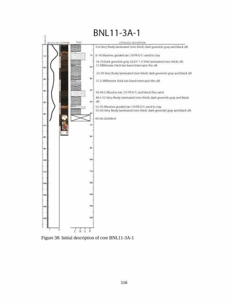
116
Figure 38: Initial description of core BNL11-3A-1

117
Figure 39: Initial description of core RAV11-1A-1

118
Figure 40: Initial description of core RAV11-1A-2

119
Figure 41: Initial description of core RAV11-2A-1

120
Figure 42: Initial description of core RAV11-3A-1

121
Figure 43: Initial description of core RAV11-4A-1

122
Figure 44: Initial description of core RPD11-1A-1

123
Figure 45: Initial description of core RPD11-1B-1

124
Figure 46: Initial description of core RPD11-1C-1

125
Figure 47: Initial description of core RPD11-2A-1

126
BIOGRAPHY OF AUTHOR
Aaron Medford was born in Hudson, NY on May 11, 1989. He moved to
Cortland, NY in 1999, where Aaron graduated Cortland Jr.-Sr. High School in 2007.
Aaron then attended Lafayette College for a liberal arts undergraduate education. He
spent a semester abroad in Leeds, England in 2009, and received a Bachelor of Science in
geology in 2011. Aaron immediately began graduate education at The University of
Maine, focusing in glacial geology. Aaron Medford is a candidate for the Master of
Science degree in Earth and Climate Sciences from The University of Maine in August
2013.