home bias in currency forecasts - university of...

1

Home Bias in Currency Forecasts*

Yu-chin Chen (University of Washington)

Kwok Ping Tsang (Virginia Tech)

Wen Jen Tsay (Academia Sinica)

This Draft: May 2010

Abstract: The "home bias" phenomenon states that empirically, economic agents often under-utilize opportunities beyond their country borders, and it is well-documented in various international pricing and purchase patterns. This bias manifests in the forms of fewer exchanges of goods and net equity-holdings, as well as less arbitrage of price differences across borders than theoretically predicted to be optimal. Our paper documents another form of home bias, where market participants appear to under-weigh information beyond their borders when making currency forecasts. Using monthly data from 1995 to 2010 for seven major exchange rates relative to the US dollar, we show that excess currency returns and the errors in investors' consensus forecasts not only depend on the interest differentials between the pair of countries, but they depend more strongly on interest rates in a broader set of countries. A global short interest differential and a global long interest differential are driving the results.

JEL Classifications: F31, G12, D84

Keywords: Survey Data, Excess Currency Returns, Global Shock

* This work is partly undertaken while the first two authors are visiting the Hong Kong Institute of Monetary Research (HKIMR). Chen: Department of Economics, University of Washington, Box 353330, Seattle, WA 98195; [email protected]. Tsang: Department of Economics, Virginia Tech, Box 0316, Blacksburg, VA, 24061; [email protected]. Tsay: Institute of Economics, Academia Sinica, Taipei, Taiwan; [email protected].

2

1. Introduction

Studies of cross-border empirics have generated various well-known puzzles that exhibit a home

bias tendency. Since McCallum (1995), the trade literature systematically observes that, ceteris

paribus, the extent of trade cross geographical locations is significantly reduced once a national

border is crossed (see Wei (1996)). On the international finance front, French and Poterba (1991)

and Tesar and Werner (1995) similarly document that agents seem to hold a disproportionally

large fraction of their equity portfolio in home assets, seemingly ignore better opportunities to

diversify risk in the broader international markets. Engel and Roger (1996) find much less price

convergence across country borders than within. While subsequent research has put forth

alternative explanations for each of these robust empirical patterns, the general observation is

that economic agents tend to under-utilize opportunities or information from beyond their home

borders.

This paper documents yet another "home bias puzzle" in forecasting currency returns.

Using a panel of data on surveyed investors' forecasts, we show that investors systematically

under-weigh information coming from the broader foreign markets, and that they could obtain

quantitatively significantly better currency forecasts had they used these foreign information

more efficiently. We show that one global short-term interest differential and one global long-

term interest differential can forecast out of sample the forecast error that will be committed by

the forecasters, outperforming the null of random walk. Forecasters are throwing away

information that can improve their forecasts.

Our empirical exploration starts from the well-known forward premium or uncovered

interest rate parity puzzle: the empirical regularity that currencies of high interest rate countries

tend to appreciate, rather than depreciate according to the foreign market efficiency condition

(UIP). Since Fama (1984), the pattern has been shown to be robust across countries and time

periods. In their survey Froot and Thaler (1990) show that most empirical studies find

coefficient on the UIP regress has the wrong sign. While various explanations have been put

forth1, we focus on explaining the failure of the UIP by the expectations biases using survey

1 Alvarez, Atkeson and Kehoe (2009), Bekaert (2006), and Lustig and Verdelhan (2007) explain the failure by a time-varying risk premium. We also have the Peso problem argument by Kaminsky (1993) the related rare events framework of Farhi and Gabaix (2009).

3

data.2 According to most of the explanations for the failure of UIP, the UIP regression (ex post

exchange rate change on the interest differential) suffers from the omitted variable problem. For

example, if risk premium is time varying and it is correlated with the interest differential, then

the UIP regression is biased. If expectations error is non-rational and is correlated with the

interest differential, again the UIP regression is biased. The goal of this paper is to document

how the expectations error can be explained by currently available variables, especially interest

differentials of other countries.

Frankel and Froot (1987, 1989) are among the first to make use of survey data to test for

rationality in the foreign exchange market. In Frankel and Froot (1987), it is found that while

actual exchange rate behaves like a random walk, it is not true for the exchange rate survey

forecast. The resulting bias in the forecast rejects rational expectations. Frankel and Froot (1989)

use survey data to account for the failure of UIP. They decompose the deviation from the UIP

into the part that is due to forecast error and the part that is due to risk premium, and find that

almost none of the deviation of the UIP can be attributed to risk premium. Chinn and Frankel

(2006) is a recent update of the two studies with more currencies and more horizons, and they

confirm the earlier results by Frankel and Froot.

This paper is related to Bacchetta, Mertens and van Wincoop (BMV, 2009) who find that

for markets where there is substantial excess return predictability, expectation errors of excess

returns (which is equivalent to forecast errors for exchange rate change) are also predictable.

Hence they find predictability of forecast errors in foreign exchange, stock and bond markets, but

not so for the money market, where there is no excess return predictability. The approach of this

paper is similar to BMV, but instead of using the country pair's own interest differential only to

predict excess return and forecast error, we emphasize 1) the informational content of term

structure by adding the long interest differential and 2) the role of a latent global factor by adding

the interest differentials of other country pairs. We find that the predictability of both excess

return and forecast error is substantially higher with the extension.

We show that considering the other interest differentials improves the consensus

forecasts both in and out of sample, which suggests that forecasters consistently neglect the

2 See Frankel and Froot (1989), Lewis (1989) and Gourinchas and Tornell (2004).

4

information contained in the interest differentials of other country pairs. We then summarize the

information in the interest differentials by extracting the first two principal components from the

group of short-term interest differentials and two from the group of long-term interest

differentials. The four principal components capture most of the movements of the interest

differentials, but we find that the first principal component in each group is enough to improve

the forecasters' performance. Factor analysis suggests the role of a few global factors, and we

conclude the paper by proposing an explanation for the forecasters' neglect of the global factors.

2. The Consensus Economics Dataset

Since 1989, Consensus Economics (CE) has been polling forecasters to obtain their forecasts for

the major macroeconomic indicators (e.g. real GDP growth, inflation, interest rates and exchange

rate) in over 70 countries. The number of forecasters varies over countries and time periods. For

most variables, forecasts are made for the current year and the following year. For example, the

survey available in March 2009 provides forecasts for the GDP growth of 2009 (December to

December) and that of 2010. For this paper we mainly make use of forecasts of exchange rates

and interest rates, which come in a different format. In each month, forecasters are asked to

predict the level of exchange rate at the 3, 12 and 24 months horizons, and the level of 3-month

and 10-year interest rates at the 3 and 12 months horizons. The survey is done usually during the

first half of the month.

With the United States as the home country, we study seven country pairs of the United

Kingdom, Japan, Canada, Singapore, Switzerland, Australia and New Zealand. Forecasts for the

first four countries are available since October 1989, and for Singapore, Switzerland, Australia

and New Zealand they are available since January 1995. Actual exchange rates on the survey

date are provided by Consensus Economics, and actual interest rates for 3-month and 10-year

maturities are obtained from the Global Financial Data database.3 All sample ends on April

2010.

3 We use the 5-year government bond rate for Singapore as the 10-year data are available for a very short sample only.

5

2.1. Properties of the Subjective Excess Currency Return

We begin with the definitions of the variables of interest. The goal of this paper is to

provide evidence for the predictability of excess return and forecast error, and we can define ex

post excess return as:

1200 (1)

The -period domestic and foreign interest rates, and , are annualized and in percentage

point. Exchange rate is defined as the US dollar price of the foreign currency, and the -period

change of its log, , is multiplied by to convert it into annual rate. For this paper we

have = 3 months. Using the survey expectations , we can rewrite (1) as:

1200 1200 (2)

We can interpret (2) as follows:

(3)

Ex post excess return is predictable either due to a predictable subjective ex ante

excess return , a predictable forecast error , or both. Though most studies focus on

coming up with theories to account for a time-varying ex ante excess return and assume

the forecast error to have a conditional mean of zero, we document below that most of the

movement of ex post excess return can be attributed to the forecast error (as in Froot and Frankel

(1989)). Next, we provide in-sample and out-sample evidence of the predictability of excess

return and forecast error . We show that a country pair's own interest differential

only has modest predictive power, but adding 1) interest differential of longer maturity (Chen

and Tsang (2009a)) and 2) interest differentials of other country pairs substantially increase the

forecasting power.

Notice that in the -period forecast error , the expectation operator refers to the

CE forecast, and it may be different from the statistical forecast , which is the rational

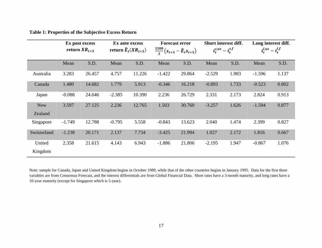
expectations forecast made using time information. The summary statistics for the three

6

variables , and are provided in Table 1. Ex post excess return has a

standard deviation many times of its mean, in contrast to the much less volatile ex ante excess

return. Due to the negative correlation between ex ante excess return and forecast error, forecast

error has a larger standard deviation than ex post excess return. We can see from Table 1 that

most of the fluctuations in ex post excess return is due to forecast error, not ex ante excess return.

Table 1 also shows the summary statistics for the interest differentials, and clearly they

are a lot less volatile than the excess returns and forecast errors. Figure 1 plots the seven short-

term (3-month) interest differentials and the long-term (mostly 10-year) interest differentials, and

their quite stable over time. Throughout most of the sample, Japan, Singapore and Switzerland

have lower interest rates than the US, while Canada, New Zealand and United Kingdom are

paying higher rates.

3. Surveyed Excess Returns, Ex Post Excess Returns and Forecast Errors

In this section we explain the movements in ex post excess returns, surveyed excess returns and

the forecast errors using 1) interest differential of the country pair, 2) short-term and long-term

interest differentials of all seven country pairs and 3) principal components extracted from the

interest differentials. We first check the in-sample fit using overlapping and non-overlapping

data, and we then see if using the principal components can improve the consensus forecasts out

of sample.4

As documented in BMV, excess returns and survey forecast errors in the currency market

are highly predictable. Fitting in sample, they find that interest differential is highly

significant in explaining forecast error and excess return for 3,6

months. We extend their result by including interest differentials of the other countries as

explanatory variables. More precisely, we consider the regression of the form, for each country

pair:

4 Our results are not driven by using the US as the home currency. The results are similar using any currency in the sample as the base currency. It clears us from the suspicion that what we will be discussing is simply "US factors".

7

, , (4)

where is either the excess return or forecast error , and is the total

number of country pairs (which is seven in this paper). As 3 is larger than the frequency of

the data, is overlapping over time. As a result, the error is serially correlated and the

-statistic and -sq of (4) using OLS will be biased upward (i.e. the results are biased toward

finding the interest differentials to be relevant).

We do two robustness checks. First, we report the -statistic and -sq using non-

overlapping quarterly data (last month of each quarter). Second, we do a simple Monte Carlo

experiment to control for the upward bias, in a manner similar to Mark (1995): 1) we regress

forecast error or excess return for each country on a constant and keep the estimated standard

error of regression , 2) we generate one step ahead forecast error or excess return from the

distribution 0, , 3) we create the 3-month ahead forecast error or excess return by the sum

, and 4) we estimate the own interest differential model or our model on the

generated data, and keep the -sq and -statistic. The null of the experiment is that excess

return or forecast error is pure random walk, and the experiment tells us the amount of bias

induced by overlapping data for each model. We run the experiment 5000 times for each

country, and subtract the mean of the generated -sq and -statistic from the actual ones to

correct for the bias. Though we have found substantial bias in the -sq, the results show that

there is no bias in the -statistic. In the results below we only report the correction for the

former statistic.

Tables 2 and 3 report the results for excess returns. First, for regressions that only use the

country pair's own interest differential, we only find some predictability, in contrast to BMvW.

Once we use non-overlapping data in Table 3 or correct for bias in the -sq, the predictability

mostly goes away. The model using all interest differentials are different: the -sq is

substantially higher and some are above 10% even after correction, and the -statistic rejects for

all country pairs the hypothesis that all the interest differentials are irrelevant. The results with

all interest differentials survive with the non-overlapping data.

8

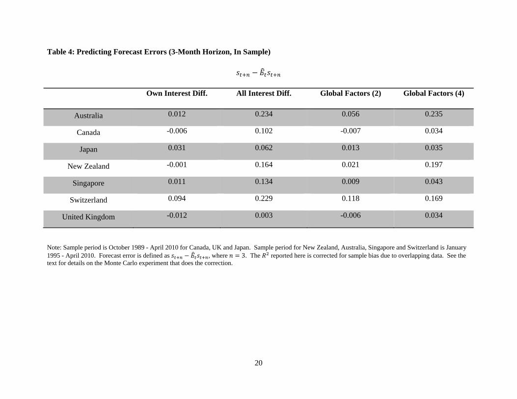
Tables 4 and 5 report the results for forecast errors. Again, we do not find as much

predictability using each country pair's own interest differential as in BMV, and the results are

even weaker with non-overlapping data and the bias correction, except perhaps Switzerland.5

Once other interest differentials are added, the in-sample fit increases substantially, in both the

overlapping and non-overlapping samples. Some of the corrected -sq’s are well above 10%.

Finally, Tables 6 and 7 report the results for the surveyed excess return.

3.1. Using Principal Components

While we have shown that using all the fourteen interest differentials is clearly preferred to using

the own interest differential, our model suffers from two problems: 1) the coefficients are hard to

interpret, and the regression may have close to perfect collinearity, and 2) the large number of

explanatory variables become a burden when we want to forecast out of sample in the next

section. Here we reduce the dimension of our explanatory variables by using the first two

principal components from the seven short interest differentials and two from the seven long

interest differentials. The four factors are plotted in Figures 1 and 2.6 The first components from

both groups are very similar to the simple average. The two first principal components look

similar as short rates and long rates usually move together, and their difference can be interpreted

as the “global slope”.

In the second-to-last column in Tables 2-7 we report the results using the first principal

components, and in the last columns we use the first and second principal components. Since the

two principal components only capture 80% of the seven interest differentials, we should expect

a worse in-sample fit. For excess return and forecast error, using 2 factors seems inadequate, but

with 4 factors the performance is quite close to the model using all the fourteen interest

differentials. In contrast, for the subjective excess return the factors perform much worse than

the interest differentials.

We can from Table 8 how the interest differentials are related to the principal

components. For the short-term interest differentials, the first principal component is positively 5 If we drop the 2008-2009 data, we obtain the strong results in BMV. The large fluctuations of most currencies over 2008 and 2009 reduce the significance of their results. 6 For both the short and long interest differentials, the first two principal components explain about 80% of the variations.

9

to the seven interest differentials positively, and accounts for 63% of their variations. The

second principal component (which, by definition, is uncorrelated to the first) only accounts for

17% of the variations, and it does not have a clear relationship with the interest differentials. It is

worth mentioning that for Singapore the interest differential loads heavily on the second

component and weakly to the first. For the long-term interest differentials, except for Singapore

all the interest differentials have a positive loading on the first principal component, and it

accounts for 57% of the variations. The second component accounts for 21% of the variations,

but again its relationship with the differentials is unclear. For Singapore the loading (which is

negative) on the first component is small, while its loading on the second component is large.

Tables 9 and 10 report the coefficients on the principal components for the last two

regressions in Tables 2-7.

3.2. Further Evidence Based on Bayesian Model Averaging (BMA)

Specification (4) is agnostic: all eight interest differentials are included for any excess return or

forecast error. The BMA method (Raftery, Madigan and Hoeting (1997), Hoeting, Madigan,

Raftery and Volinsky (1999)) allows us to ask the question: given the data, what is the posterior

probability that each interest differential should be included in a model for predicting forecast

error or excess return? While we focus on in-sample fit in this section, see Wright (2008) for

out-example exchange rate forecast using BMA.

Tables 11-13 show the BMA results for excess returns, forecast errors and the subjective

excess returns. The posterior inclusion probabilities can be interpreted as the probability that a

variable is included in the model, given the data. For example, if 0| 50%, it

means the probability that a variable (for which the coefficient is ) is larger than 50%. Or, it is

more likely than not that the variable is in the model. There is some theoretical support for

emphasizing variables that have inclusion probability larger than 50%: the "median probability

model", which includes all variables with an inclusion probability larger than 50%, is often the

optimal predictive model (Barbieri and Berger 2004). According to Tables 6 and 7, even under

the conservative requirement that only variables with an inclusion probability larger 80% are

10

included, many interest differentials are found to be important for predicting forecast error and

excess return.

4. Out-Sample Forecasting

As established by Meese and Rogoff (1983), good in-sample fit does not imply good out-sample

prediction. To further support our results so far, we carry out a horse race in predicting 3-month

exchange rate change between using the eight interest differentials and using the CE forecasts.

First, we regress the actual 3-month exchange rate change on each of the eight interest

differentials recursively, using the 5 years of data since January 1995 (so that all country pairs

start at the same period). Next, we generate the first out-sample forecast from each of the eight

regressions, and we take the average of the eight forecasts as our combined out-sample forecast.

As explained in Timmerman (2006), simple combinations of forecasts dominate more

complicated methods that aim at finding the optimal weights. The combined forecasting method

is more efficient than having all eight interest differentials in a single regression as in (4).

Table 14 reports the results. We consider two forecast periods: the first period is March

2000 - October 2007 (i.e. the first forecast is for the exchange rate change between March 2000

and June 2000), roughly before the 2008-2009 financial crisis; the second period is March 2000 -

January 2010 (i.e. the last forecast is for the exchange rate change between January 2010 and

April 2010), which includes the financial crisis. In the first period, we significantly beat the CE

forecasts for Australia, Canada, and Japan. We also forecast better than CE for Switzerland and

UK, though not significantly so, and we perform worse than CE for Singapore. In the second

period, during which we have large fluctuations in the all the currencies, our combined forecast

still performs reasonably well comparing to the CE forecasts, and we beat the CE forecasts

significantly for Australia and Japan.

On the other hand, using the country's own interest differential forecasts poorly

comparing to the CE forecasts. For both sample periods and for most currencies the interest

differential forecast has a higher RMSE than the CE forecast, sometimes significantly so. That is,

a forecaster who uses a simple "UIP model" will do worse than a group of professional

forecasters.

11

We do a second out-sample exercise as a robustness check, making use of the principal

components. We compare the model that forecast error is random walk (possibly serially

correlated due to the overlapping data) with the model that forecast error is a function of the

principal components. A more parsimonious model, the random walk, is the null and the

alternative is a larger model with principal components. The question we are asking is then: are

the CE forecasters neglecting the global factors or, if they do look at the global factors, using

them "wrongly"? Clark and West (2007) propose a test that takes into the account the

uncertainty involved in estimating the extra coefficients for the principal components. Table 15

gives the results using one principal component for the short-term differentials and one for the

long-term. The random walk null is rejected for most currencies for both sample periods. When

we move to four principal components in Table 16, the results are much less significant,

suggesting that a model for the forecast error may contain two factors but not four.

5. Discussion

What have we seen so far? First, the short and long interest differentials are powerful predictor

for excess returns, forecast errors and surveyed excess returns. While using a currency pair's

own interest differential is not enough, we find that extracting one or two principal components

from each of the short and long interest differentials is enough to capture the in-sample fit of

using all the differentials. Second, we learn that either the differentials or their principal

components are useful for improving upon the CE forecasts out of sample, while a currency

pair's own interest differential does not help at all. What do these findings imply?

Forecasters do not neglect the global factors, but they are using it differently from what

the data would suggest.

One may be suspicious of the quality of the quality of the exchange rate forecast. The

forecaster could just give a random guess, or give a biased answer under self interest (e.g. predict

a rise in UK pound when the forecaster or the forecaster's institution is holding UK pound). For

either of the two reasons we have measurement error in the forecast, and the forecast cannot

perfectly measure the "market's forecast". Since we do not use survey data in the right-hand

side, a random measurement error that is uncorrelated with the interest differentials will just

12

reduce the in-sample fit. Mechanically, for the true forecast error (the one using true "market's

forecast") to be unpredictable but the survey forecast error to be predictable, we need the

measurement error to be correlated with the interest differentials. As it is hard to argue for such

a measurement error, and it is unreasonable to attribute all of our results to it, we conclude that

our strong results are not due to the bad survey data.

What explain the results? As suggested in BMV, there are two types of explanations.

First is to argue that, due to learning or other non-rational expectations mechanisms, forecast

error is predictable and it results in a predictable excess return. Gourinchas and Tornell (2004)

argue for this causal relationship. Second is to argue that there is a third factor contributing to

the predictability of both variables. For example, Bacchetta and van Wincoop (2009) suggest

that if the gain of active trading is small comparing to the fees, portfolio decision will be

infrequent and deviation from UIP will be left uncorrected.

We offer a related explanation for our results. Suppose the term structure in each country

is driven by both domestic factors and global factors, with the domestic factors reflecting

expectations of domestic macroeconomic fundamentals and the global factors reflecting those of

global fundamentals. If the investors cannot distinguish between the two types of factors

perfectly, and that they need to learning about the processes of the factors, expectations can be

non-rational and can explain the predictability of the forecast error.

6. Conclusion

Excess return is predictable mainly because exchange rate forecast error is predictable.

Exchange rate forecasts from the Consensus Economics dataset fail the rationality significantly:

current interest differentials can explain future forecast errors, both in and out of sample.

We explain our results by the presence of latent global factors contained in the interest

differentials that investors do not observe directly. If investors cannot distinguish between the

domestic factors and global factors perfectly, and that they need to learn about the processes of

the factors, then forecast can be non-rational and can explain the predictability of the forecast

13

error. We leave a more careful modeling of the learning mechanisms for our other paper in

progress (Chen, Tsang and Tsay (2010)).

14

REFERENCES

[1] Alvarez, Fernando, Andrew Atkeson and Patrick J. Kehoe (2009): “Time-Varying Risk,

Interest Rates, and Exchange Rates in General Equilibrium,” Review of Economic Studies,

Volume 76, Number 3, pp. 851-878(28).

[2] Bacchetta, Philippe and Eric van Wincoop, "Infrequent Portfolio Decisions: A Solution to

the Forward Discount Puzzle," 2009, forthcoming American Economic Review.

[3] Bacchetta, Philippe, Elmar Mertens and Eric van Wincoop, " Predictability in Financial

Markets: What do Survey Expectations Tell Us?" Journal of International Money and

Finance Volume 28, Issue 3, April 2009, Pages 406-426.

[4] Barbieri, Maria M. and James O. Berger, "Optimal Predictive Model Selection," Annals

of Statistics, Volume 32, Number 3 (2004), 870-897.

[5] Bekaert, Geert (1996): “The Time Variation of Risk and Return in Foreign Exchange

Markets: A General Equilibrium Perspective,” Review of Financial Studies, Vol. 9, No. 2, pp.

427-470.

[6] Chen, Yu-chin and Kwok Ping Tsang, "What Does the Yield Curve Tell Us About

Exchange Rate Predictability?" working paper 2009.

[7] Chen, Yu-chin and Kwok Ping Tsang, "A Macro-Finance Approach to Nominal Exchange

Rate Determination" working paper 2009.

[8] Chen, Yu-chin, Kwok Ping Tsang and Wen Jen Tsay, "Monetary Policy, Learning, and

Global Risk Factors," working paper 2010.

[9] Devereux, Michael B., Gregor W. Smith and James Yetman, "Consumption and Real

Exchange Rates in Professional Forecasts," working paper, 2009.

[10] Diebold, Francis X., C. Li and Vivian Yue, "Global Yield Curve Dynamics and

Interactions: A Generalized Nelson-Siegel Approach," Journal of Econometrics, 146, 351-

363.

[11] Engel, Charles and John H. Rogers (1996): “How Wide Is the Border?” American

Economic Review, Vol. 86, No. 5, pp. 1112-1125.

[12] Engel, Charles, Nelson C. Mark and Kenneth D. West, "Exchange Rate Models are

not as Bad as You Think," 381-443 in NBER Macroeconomics Annual 2007, D. Acemoglu,

K. Rogoff and M. Woodford (eds.), Chicago, University of Chicago Press.

15

[13] Fama, Eugene F. (1984): “Forward and spot exchange rates,” Journal of Monetary

Economics, Volume 14, Issue 3, Pages 319-338.

[14] Farhi, Emmanuel and Xavier Gabaix, "Rare Disasters and Exchange Rates," working

paper, 2009.

[15] Frankel, Jeffery A. and Menzie Chinn, "More Survey Data on Exchange Rate

Expectations: More Currencies, More Horizons, More Tests," in W. Allen and D. Dickinson

(editors), Monetary Policy, Capital Flows and Financial Market Developments in the Era of

Financial Globalisation: Essays in Honour of Max Fry, (Routledge, 2002), pp. 145-67.

[16] Frankel, Jeffery A. and Kenneth A. Froot, "Using Survey Data to Test Propositions

Regarding Exchange Rate Expectations," American Economic Review, Vol. 77, No. 1 (March

1987), p. 133-153.

[17] French, Kenneth R. and James M. Poterba (1991): “Investor Diversification and

International Equity Markets,” American Economic Review, Vol. 81, No. 2, Papers and

Proceedings of the Hundred and Third Annual Meeting of the American Economic

Association, pp. 222-226.

[18] Froot, Kenneth A. and Jeffery A. Frankel, "Forward Discount Bias: Is it an Exchange

Risk Premium?" Quarterly Journal of Economics, Vol. 104, No. 1 (February 1989), p. 139-

161.

[19] Gourinchas, Pierre-Olivier and Aaron Tornell, "Exchange Rate Puzzles and Distorted

Beliefs," Journal of International Economics, 64 (2004), 303-333.

[20] Kaminsky, Graciela (1993): “Is There a Peso Problem? Evidence from the Dollar/Pound

Exchange Rate, 1976-1987,” American Economic Review, Vol. 83, No. 3, pp. 450-472.

[21] Lahiri, Kajal, G. Isikler and P. Loungani, "How Quickly Do Forecasters Incorporate

News? Evidence from Cross-country Surveys", Journal of Applied Econometrics, 21, 2006,

703-725.

[22] Lewis, Karen K. (1989): “Changing Beliefs and Systematic Rational Forecast Errors with

Evidence from Foreign Exchange,” American Economic Review, Vol. 79, No. 4, pp. 621-

636.

[23] Lustig, Hanno, and Adrien Verdelhan. 2007. "The Cross Section of Foreign Currency

Risk Premia and Consumption Growth Risk." American Economic Review, 97(1): 89–117.

16

[24] Lustig, Hanno, Nikolai Roussanov and Adrien Verdelhan, " Common Risk Factors in

Currency Markets," NBER Working Papers 14082 (2008), National Bureau of Economic

Research, Inc.

[25] Mark, Nelson C. (1995): “Exchange Rates and Fundamentals: Evidence on Long-Horizon

Predictability,” American Economic Review, Vol. 85, No. 1), pp. 201-218.

[26] McCallum, John (1995): “National Borders Matter: Canada-U.S. Regional Trade Patterns,”

American Economic Review, Vol. 85, No. 3 (Jun., 1995), pp. 615-623.

[27] Meese, Richard A. and Kenneth Rogoff (1983), "Empirical Exchange Rate Models of the

Seventies: Do They Fit Out of Sample?" Journal of International Economics, 14, 3-24.

[28] Piazzesi, Monika and Martin Schneider, "Trend and cycle in Bond Premia," working

paper 2009.

[29] Raftery, Adrian E., David Madigan, and Jennifer A. Hoeting (1997), “Bayesian Model

Averaging for Linear Regression Models,” Journal of the American Statistical Association,

92, 179-191.

[30] Hoeting, Jennifer A., David Madigan, Adrian E. Raftery, and Chris T. Volinsky

(1999), "Bayesian Model Averaging: A Tutorial," Statistical Science, Vol. 14, Number 4,

382-417.

[31] Sala-i-Martin, X., G. Doppelhofer and R.I. Miller. (2004), "Determinants of Long-Term

Growth: A Bayesian Averaging of Classical Estimates (BACE) Approach," American

Economic Review 94, 813-835.

[32] Stock, James H. and Mark W. Watson, "Combination Forecasts of Output Growth in a

Seven Country Data Set," Journal of Forecasting, 23 (2004), 405-430.

[33] Tesar, Linda L. and Ingrid M. Werner (1995): “Home bias and high turnover,” Journal

of International Money and Finance, Volume 14, Issue 4, Pages 467-492

[34] Timmermann, Allan, "Forecast Combinations," in: Handbook of Economic Forecasting,

Clive Granger, Graham Elliott and Allan Timmermann, eds. (Amsterdam: North Holland, vol.

1, 2006).

[35] Wei, Shang-Jin (1996): “Intra-National versus International Trade: How Stubborn are

Nations in Global Integration?” NBER working paper no. 5531.

[36] Wright, Jonathan H., "Bayesian Model Averaging and Exchange Rate Forecasts,"

Journal of Econometrics, Volume 146, Issue 2, October 2008, p. 329-341.

17

Table 1: Properties of the Subjective Excess Return

Ex post excess return

Ex ante excess return

Forecast error

Short interest diff. , ,

Long interest diff. , ,

Mean S.D. Mean S.D. Mean S.D. Mean S.D. Mean S.D.

Australia 3.283 26.457 4.757 11.226 -1.422 29.864 -2.529 1.983 -1.596 1.137

Canada 1.480 14.682 1.779 5.913 -0.346 16.218 -0.893 1.733 -0.523 0.802

Japan -0.088 24.646 -2.385 10.390 2.236 26.729 2.331 2.173 2.824 0.913

New

Zealand

3.597 27.125 2.236 12.765 1.503 30.760 -3.257 1.626 -1.594 0.877

Singapore -1.749 12.788 -0.795 5.558 -0.843 13.623 2.040 1.474 2.399 0.827

Switzerland -1.238 20.171 2.137 7.734 -3.425 21.994 1.027 2.172 1.816 0.667

United

Kingdom

2.358 21.615 4.143 6.943 -1.886 21.806 -2.195 1.947 -0.867 1.076

Note: sample for Canada, Japan and United Kingdom begins in October 1989, while that of the other countries begins in January 1995. Data for the first three variables are from Consensus Forecast, and the interest differentials are from Global Financial Data. Short rates have a 3-month maturity, and long rates have a 10-year maturity (except for Singapore which is 5-year).

18

Table 2: Predicting Excess Returns (3-Month Horizon, In Sample)

1200

Own Interest Diff. All Interest Diff. Global Factors (2) Global Factors (4)

Australia 0.008 0.143 0.034 0.135

Canada -0.005 0.039 -0.019 -0.010

Japan 0.074 0.049 0.073 0.081

New Zealand -0.008 0.044 0.010 0.086

Singapore 0.047 0.133 0.022 0.046

Switzerland 0.062 0.118 0.052 0.070

United Kingdom 0.010 0.033 -0.004 0.027

Note: Sample period is October 1989 - April 2010 for Canada, UK and Japan. Sample period for New Zealand, Australia, Singapore and Switzerland is January 1995 - April 2010. Excess return is defined as . The reported here is corrected for sample bias due to overlapping data. See the text for details on the Monte Carlo experiment that does the correction.

19

Table 3: Predicting Excess Returns (3-Month Horizon, In Sample, Non-overlapping Data)

1200


Australia 0.007 0.140 0.047 0.145

Canada -0.011 0.001 -0.017 -0.018

Japan 0.089 0.079 0.093 0.089

New Zealand -0.015 0.006 0.026 0.062

Singapore 0.082 0.191 0.024 0.054

Switzerland 0.053 0.098 0.036 0.041

United Kingdom 0.003 -0.049 0.003 0.042

Note: Sample period is October 1989 - April 2010 for Canada, UK and Japan. Sample period for New Zealand, Australia, Singapore and Switzerland is January 1995 - April 2010. Excess return is defined as . Non-overlapping data are constructed by picking the last month of each quarter.

20

Table 4: Predicting Forecast Errors (3-Month Horizon, In Sample)


Australia 0.012 0.234 0.056 0.235

Canada -0.006 0.102 -0.007 0.034

Japan 0.031 0.062 0.013 0.035

New Zealand -0.001 0.164 0.021 0.197

Singapore 0.011 0.134 0.009 0.043

Switzerland 0.094 0.229 0.118 0.169

United Kingdom -0.012 0.003 -0.006 0.034

Note: Sample period is October 1989 - April 2010 for Canada, UK and Japan. Sample period for New Zealand, Australia, Singapore and Switzerland is January 1995 - April 2010. Forecast error is defined as , where 3. The reported here is corrected for sample bias due to overlapping data. See the text for details on the Monte Carlo experiment that does the correction.

21

Table 5: Predicting Forecast Errors (3-Month Horizon, In Sample, Non-overlapping Data)


Australia 0.005 0.198 0.068 0.218

Canada -0.012 0.063 -0.018 -0.001

Japan 0.019 0.086 0.011 0.020

New Zealand -0.011 0.068 0.039 0.133

Singapore 0.039 0.194 0.013 0.060

Switzerland 0.091 0.222 0.115 0.152

United Kingdom -0.012 -0.096 -0.010 0.051

Note: Sample period is October 1989 - April 2010 for Canada, UK and Japan. Sample period for New Zealand, Australia, Singapore and Switzerland is January 1995 - April 2010. Forecast error is defined as , where 3. The reported here is corrected for sample bias due to overlapping data. See the text for details on the Monte Carlo experiment that does the correction. Non-overlapping data are constructed by picking the last month of each quarter.

22

Table 6: Predicting Surveyed Excess Return (3-Month Horizon, In Sample)

1200


Australia -0.008 0.252 0.024 0.136

Canada -0.012 0.139 0.005 0.091

Japan 0.012 0.223 0.049 0.064

New Zealand 0.002 0.323 0.016 0.151

Singapore 0.025 0.291 0.037 0.032

Switzerland 0.033 0.197 0.091 0.146

United Kingdom 0.196 0.253 0.184 0.184

Note: Sample period is October 1989 - April 2010 for Canada, UK and Japan. Sample period for New Zealand, Australia, Singapore and Switzerland is January

1995 - April 2010. Surveyed excess return is defined as , where 3. The reported here is corrected for sample bias due to

overlapping data. See the text for details on the Monte Carlo experiment that does the correction.

23

Table 7: Predicting Surveyed Excess Return (3-Month Horizon, In Sample, Non-overlapping Data)

1200


Australia -0.016 0.344 0.052 0.105

Canada -0.010 0.154 -0.018 0.006

Japan 0.051 0.330 0.088 0.084

New Zealand -0.002 0.361 -0.010 0.030

Singapore 0.013 0.398 0.064 0.037

Switzerland 0.041 0.216 0.122 0.134

United Kingdom 0.140 0.220 0.125 0.199

Note: Sample period is October 1989 - April 2010 for Canada, UK and Japan. Sample period for New Zealand, Australia, Singapore and Switzerland is January

1995 - April 2010. Surveyed excess return is defined as , where 3. The reported here is corrected for sample bias due to

overlapping data. See the text for details on the Monte Carlo experiment that does the correction. Non-overlapping data are constructed by picking the last

month of each quarter.

24

Table 8: Loadings of the Interest Differentials on the Factors

Short-Term Principal Component 1

(63%)

Short-Term Principal Component 2

(17%)

Long-Term Principal

Component 1

(57%)

Long -Term Principal

Component 2

(21%)

Australia 0.413 -0.092 0.466 -0.062

Canada 0.412 -0.284 0.422 -0.239

Japan 0.426 0.296 0.402 0.340

New Zealand 0.363 -0.146 0.344 0.231

Singapore 0.126 0.842 -0.244 0.635

Switzerland 0.398 0.188 0.223 0.590

United Kingdom 0.415 -0.239 0.465 -0.134

Note: We extract two principal components each from 1) the seven short-term interest differentials and 2) the seven long-term interest differentials. The percentage in the first row is the proportion of variations in the variables explained by that component.

25

Table 9:Ex Post Excess Return, Forecast Error, and Surveyed Excess Return: Loadings on the Factors (2 Factors)

Ex Post Excess Return Forecast Error Surveyed Excess Return Short PC Long PC Short PC Long PC Short PC Long PC

Australia -0.852 (1.657) -4.181 (1.928) 0.388 (1.848) -6.716* (2.152) -1.275 (0.707) 2.517* (0.824)

Canada 0.477 (0.857) -0.925 (0.904) 0.686 (0.942) -1.592 (0.993) -0.200 (0.341) 0.657 (0.359)

Japan -6.325*** (1.372) 4.133* (1.447) -4.443* (1.537) 3.411 (1.620) -1.863* (0.587) 0.704 (0.618)

New

Zealand -0.879 (1.698) -4.279** (1.977) -0.358 (1.897) -6.598* (2.208) -0.583 (0.807) 2.301 (0.940)

Singapore -1.589 (0.806) -0.381 (0.938) -0.442 (0.864) -1.534 (1.006) -1.180** (0.347) 1.142 (0.405)

Switzerland -2.762 (1.250) -1.392 (1.455) -3.541 (1.316) -2.678 (1.532) 0.775 (0.469) 1.282 (0.546)

United

Kingdom -2.544 (1.253) 1.711 (1.321) -2.002 (1.265) 2.777 (1.334) -0.502 (0.363) -1.106* (0.383)

Note: The coefficients and standard errors (in parentheses) are for the factors in the third regression (2 factors) reported in Tables 2-7. To correct for overlapping data problem, we use the corrected critical values for the -statistics: 2.86 for 10% (*), 3.40 for 5% (**) and 4.04 for 1% (***) (which is equivalent to divide the -statistic by the root of the horizon of the LHS, which is 3).

26

Table 10a: Ex Post Excess Return, Forecast Error, and Surveyed Excess Return: Loadings on the Factors (4 Factors)

Ex Post Excess Return Short PC 1 Long PC 1 Short PC 2 Long PC 2

Australia 6.755* (2.333) -9.007*** (2.099) -12.985*** (3.093) 0.274 (2.286)

Canada 1.390 (1.085) -2.129 (1.138) -2.442 (1.230) 0.447 (1.089)

Japan -6.903** (1.737) 4.132 (1.822) -3.254 (1.969) 3.356 (1.743)

New

Zealand 3.859 (2.461) -7.468** (2.214) -11.135** (3.263) 2.769 (2.412)

Singapore 0.651 (1.185) -1.690 (1.066) -1.970 (1.571) -1.501 (1.161)

Switzerland -0.759 (1.845) -2.800 (1.660) -5.684 (2.447) 2.003 (1.808)

United

Kingdom -1.289 (1.568) 1.188 (1.646) 3.769 (1.779) -4.787* (1.574)

Note: The coefficients and standard errors (in parentheses) are for the factors in the fourth regression (4 factors) reported in Tables 2-7. To correct for overlapping data problem, we use the corrected critical values for the -statistics: 2.86 for 10% (*), 3.40 for 5% (**) and 4.04 for 1% (***) (which is equivalent to divide the -statistic by the root of the horizon of the LHS, which is 3).

27

Table 10b: Ex Post Excess Return, Forecast Error, and Surveyed Excess Return: Loadings on the Factors (4 Factors)

Forecast Error Short PC 1 Long PC 1 Short PC 2 Long PC 2

Australia 11.900*** (2.474) -13.932*** (2.226) -18.224*** (3.281) -0.803 (2.425)

Canada 2.860 (1.173) -4.130 (1.231) -3.752 (1.330) -0.498 (1.177)

Japan -5.227 (1.932) 3.338 (2.028) -4.865 (2.191) 4.893 (1.939)

New

Zealand 9.341** (2.613) -12.826*** (2.351) -17.804*** (3.465) 1.413 (2.561)

Singapore 2.279 (1.265) -3.132 (1.138) -2.524 (1.677) -1.711 (1.240)

Switzerland -0.070 (1.902) -5.074* (1.711) -9.126** (2.522) 2.855 (1.864)

United

Kingdom -1.069 (1.576) 2.718 (1.653) 4.874 (1.787) -5.129* (1.581)


28

Table 10c: Ex Post Excess Return, Forecast Error, and Surveyed Excess Return: Loadings on the Factors (4 Factors)

Surveyed Excess Return Short PC 1 Long PC 1 Short PC 2 Long PC 2

Australia -4.944*** (0.988) 4.713*** (0.887) 4.480** (1.265) 1.345 (0.961)

Canada -1.456** (0.414) 1.986*** (0.434) 1.301 (0.460) 0.933 (0.415)

Japan -1.703 (0.740) 0.836 (0.775) 1.724 (0.822) -1.564 (0.741)

New

Zealand -5.203*** (1.110) 5.060*** (0.997) 5.540** (1.421) 1.781 (1.080)

Singapore -1.528* (0.518) 1.336* (0.465) 0.163 (0.663) 0.353 (0.504)

Switzerland -0.610 (0.675) 2.191** (0.606) 3.142** (0.864) -0.745 (0.657)

United

Kingdom -0.281 (0.461) -1.419* (0.483) -0.726 (0.513) 0.216 (0.462)


29

Table 11: Bayesian Model Averaging (BMA) Posterior Results (Excess Return )

Australia

Canada

Japan New Zealand

Singapore Switzerland United Kingdom

Short

Australia 36.5 8.8 13.7 9.5 5.3 44.1 4.5

Canada 2.3 57 80.2 4 96.2 24.2 6

Japan 4.2 26.1 14.6 8.1 9.2 0.9 9.9

New Zealand 5.1 24.5 5.7 5.6 17.4 98.7 4

Singapore 100 23.7 84.5 96.9 15.3 90.2 97.3

Switzerland 11.2 4.9 24.2 4.2 3.9 14.4 6.8

UK 99.1 98.2 4.9 96.8 95.9 97.5 71.6

Australia 7.2 6.1 4 4.3 12.8 7.2 4.2

Long

Canada 100 27.5 9.2 100 4.1 23.7 96.4

Japan 6.6 0.5 1.9 4.1 4 82.8 3.8

New Zealand 18.5 99.6 15.3 1.4 96.2 25.7 15.2

Singapore 7.3 0.7 7.1 4.1 88.7 2.8 3.3

Switzerland 6.5 25.1 71.2 11.4 93.9 26.1 99.8

UK 3.8 6.1 6.7 3.6 8.9 1 4.3

Note: The numbers reported are posterior probabilities (in percentage point) that the coefficient is zero. Probabilities higher than 80% are in bold.

30

Table 12: Bayesian Model Averaging (BMA) Posterior Results (Forecast Error )

Australia

Canada

Japan New Zealand


Short

Australia 93.5 1.8 71.1 95.1 37.8 98.9 4.9

Canada 28.9 12.9 96.2 5.5 92.5 18.5 6.8

Japan 11.7 93.9 39.4 46.6 8.7 11.3 5.4

New Zealand 3.8 43.8 8.3 3.5 4.6 99.4 0.2

Singapore 98.3 1.6 63.7 96.8 7.2 93.7 98.3

Switzerland 11.9 19.1 0.5 7.1 6.6 3.4 4.2

UK 56.1 100 24.5 12.5 96.5 81 20.2

Australia 27.6 5.3 2.9 94.4 6.9 11 5

Long

Canada 63.4 6.6 0.6 14.4 14.7 38.3 87.7

Japan 94.1 6.3 49.3 25.8 14.6 36.6 4.4

New Zealand 40.7 100 26.5 1.4 99.3 95.3 1.1

Singapore 29.6 6.4 5.5 3.7 76.3 30.7 3.4

Switzerland 46 27.6 16.5 29 87.2 3.3 99.8

UK 5.7 4 4.9 2.3 28.2 4.5 23.5


31

Table 13: Bayesian Model Averaging (BMA) Posterior Results (Subjective Excess Return )

Australia

Canada

Japan New Zealand


Short

Australia 76.6 3.2 72.7 24.5 100 82.7 50.1

Canada 14.5 10.7 5.4 13.3 2.4 49.1 10.4

Japan 35 24.6 87.2 26.8 100 100 77.7

New Zealand 5.4 6.1 99.1 43.9 4.4 12 15.8

Singapore 2.3 5.8 9.3 17.7 100 2.1 25.3

Switzerland 15.9 0.6 81.3 6.1 3.3 91.4 4

UK 11.3 96 5.7 2.8 11.8 3.4 8.3

Australia 9.2 100 10.4 15.9 5.1 2.9 5.1

Long

Canada 39.9 98.9 100 75.1 2.2 33.4 93.4

Japan 100 83.9 99.7 100 14.5 3.4 1.9

New Zealand 3 3.2 13.6 3.4 15.8 89.1 16.2

Singapore 25.7 3.2 6.1 3.7 39.8 5.7 1.7

Switzerland 86.5 2.8 99 98.6 14.2 5.8 1.8

UK 28.2 8.3 6.3 63.1 99.8 62.6 100


32

Table 14: Do the Interest Differentials Beat the Consensus Forecasts? Last Forecast Made For: Jan 2010-April 2010

RMSE (own/CE) Diebold-Mariano -value RMSE (all/CE) Diebold-Mariano -value

Australia 0.944 0.342 0.900* 0.098

Canada 0.920* 0.060 0.929 0.102

Japan 1.617** 0.026 0.904* 0.066

New Zealand 0.943 0.421 0.895 0.194

Singapore 1.026 0.788 0.930 0.390

Switzerland 1.081 0.386 0.957 0.451

UK 1.018 0.632 1.012 0.758

Last Forecast Made For: Oct 2007-Jan 2008

RMSE (own/CE) Diebold-Mariano -value RMSE (all/CE) Diebold-Mariano -value Australia 1.005 0.961 0.829** 0.043

Canada 0.915** 0.047 0.920** 0.049

Japan 1.821** 0.014 0.851** 0.029

New Zealand 1.005 0.955 0.848 0.113

Singapore 1.263* 0.053 1.086 0.332

Switzerland 1.121 0.325 0.977 0.753

UK 1.044 0.361 0.981 0.686

33

Table 15: Out-Sample Forecasting for 3-Month Forecast Error (2 factors)

Forecast Comparison End Period

May 2009 October 2007

CW Statistic p-value CW Statistic p-value

Australia 361.279** 0.021 167.853** 0.043

Canada 99.247* 0.061 32.925 0.175

New Zealand 104.261* 0.096 162.596** 0.042

Japan 379.654** 0.014 272.126** 0.019

Singapore 30.558** 0.047 12.875 0.139

Switzerland 160.399*** 0.010 137.368** 0.037

United Kingdom -11.686 0.381 1.832 0.480

Note: Starting with the 5 years of data since January 1995, we regress recursively the 3-month forecast error on the factors. We consider two ending periods, the first (October 2007) is before the 2008-2009 financial crisis while the second is after. The Clark-West (2007) statistics are reported, and a positive number means the test is in favor of the model that the error depends on the factors instead of a random walk. The -value tells us whether the preference of our model is statistically significant. * is for 10%, ** is for 5% and *** is for 1%.

34

Table 16: Out-Sample Forecasting for 3-Month Forecast Error (4 factors)

Forecast Comparison End Period

May 2009 October 2007

CW Statistic p-value CW Statistic p-value

Australia 626.569* 0.095 101.901 0.131

Canada 209.660* 0.052 21.715 0.312

New Zealand -9.981 0.462 90.602 0.199

Japan 647.881* 0.067 184.239* 0.080

Singapore 37.777 0.257 -9.860 0.182

Switzerland 154.491 0.138 155.703* 0.070

United Kingdom -71.779 0.232 37.826 0.154

Note: Starting with the 5 years of data since January 1995, we regress recursively the 3-month forecast error on the factors. We consider two ending periods, the first (October 2007) is before the 2008-2009 financial crisis while the second is after. The Clark-West (2007) statistics are reported, and a positive number means the test is in favor of the model that the error depends on the factors instead of a random walk. The -value tells us whether the preference of our model is statistically significant. * is for 10%, ** is for 5% and *** is for 1%.

35

Figure 1: Short-Term and Long-Term Interest Differentials

-12

-8

-4

0

4

8

90 92 94 96 98 00 02 04 06 08

Australia CanadaJapan New ZealandSingapore SwitzerlandUnited Kingdom

-6

-4

-2

0

2

4

6

90 92 94 96 98 00 02 04 06 08

Australia CanadaJapan New ZealandSingapore SwitzerlandUnited Kingdom

36

Figure 1: First and Second Principal Components for Short Interest Differentials

-5

-4

-3

-2

-1

0

1

2

3

4

90 92 94 96 98 00 02 04 06 08

First Principal Component

-3

-2

-1

0

1

2

3

4

90 92 94 96 98 00 02 04 06 08

Second Principal Component

37

Figure 2: First and Second Principal Components for Long Interest Differentials

-6

-4

-2

0

2

4

90 92 94 96 98 00 02 04 06 08

First Principal Component

-4

-3

-2

-1

0

1

2

3

90 92 94 96 98 00 02 04 06 08

Second Principal Component

home bias in currency forecasts - university of...

Documents