home.cscamm.umd.edu · z. angew. math. phys. (2020) 71:29 c 2020 springer nature switzerland ag ...
TRANSCRIPT
Z. Angew. Math. Phys. (2020) 71:29 c© 2020 Springer Nature Switzerland AGhttps://doi.org/10.1007/s00033-020-1250-8
Zeitschrift fur angewandteMathematik und Physik ZAMP
Entropy-stable schemes for relativistic hydrodynamics equations
Deepak Bhoriya and Harish Kumar
Abstract. In this article, we propose high-order finite difference schemes for the equations of relativistic hydrodynamics,which are entropy stable. The crucial components of these schemes are a computationally efficient entropy conservativeflux and suitable high-order entropy dissipative operators. We first design a higher-order entropy conservative flux. For theconstruction of appropriate entropy dissipative operators, we derive entropy scaled right eigenvectors. This is then usedwith ENO-based sign-preserving reconstruction of scaled entropy variables, which results in higher-order entropy-stableschemes. Several numerical results are presented up to fourth order to demonstrate entropy stability and performance ofthese schemes.
Mathematics Subject Classification. 65M08, 65M12.
Keywords. Relativistic hydrodynamics, Symmetrization, Entropy stability, Finite difference scheme.
Contents
1. Introduction2. Equations of relativistic hydrodynamics3. Entropy-stable numerical schemes
3.1. Entropy conservative schemes3.1.1. Entropy conservative flux3.1.2. Higher-order entropy conservative flux
3.2. Entropy-stable schemes3.3. High-order diffusion operators3.4. Semi-discrete entropy stability3.5. Time discretization
4. Numerical results4.1. One-dimensional test cases
4.1.1. Accuracy test4.1.2. Isentropic smooth flows4.1.3. Riemann problem 14.1.4. Riemann problem 24.1.5. Riemann problem 34.1.6. Density perturbation test case4.1.7. Blast waves test case
4.2. Two-dimensional test cases4.2.1. Two-dimensional Riemann problem 14.2.2. Two-dimensional Riemann problem 24.2.3. Two-dimensional Riemann problem 34.2.4. Two-dimensional Riemann problem 44.2.5. Two-dimensional Riemann problem 5
0123456789().: V,-vol

29 Page 2 of 29 D. Bhoriya and H. Kumar ZAMP
5. ConclusionAcknowledgementsAppendix A. Computation of primitive variablesAppendix B. Entropy scaled right eigenvectorsReferences
1. Introduction
The equations of relativistic hydrodynamics are used to model astrophysical flows when the fluid ismoving with speed comparable to the speed of light, or the flow is under the influence of large gravitationalpotentials such that relativistic effects cannot be ignored. Some examples are gamma-ray burst, relativisticjets from Galactic sources, core-collapse supernovae and extragalactic jets from active Galactic nuclei (see[5,6,20,27,39]).
In this article, we consider the equations of special relativistic hydrodynamics (RHD henceforth) withthe ideal equation of state. The system of equations is hyperbolic conservation laws. So, the solutions ofthe system can exhibit discontinuities, even for the smooth initial data (see [15]). Therefore, we considerweak solutions of the systems which are characterized by the Rankine–Hugoniot jump condition acrossthe discontinuities. However, the weak solutions of the system can be non-unique; hence, an additionalcriterion in the form of entropy inequality is imposed to choose the physically appropriate solution.However, more recently, it has been shown that even the entropy-stable solutions are not unique (see [9]).Still, entropy stability is one of the few nonlinear stability estimates available for the solutions.
Due to nonlinearity in the flux, the analytic study of the equations is difficult. Hence, we rely oncomputational methods for various applications. The computational methods for hyperbolic conservationlaws are often based on the finite volume (or finite difference) methods. These methods are based onevolving the cell averages of the state variables by approximating the numerical fluxes across the cellinterfaces. Higher order is achieved by reconstructing the solution at the cell edges, using TVD-, ENO-and WENO-based approximations (see [13,17,19,32]). To prove the entropy stability of these schemes is,however, highly non-trivial, especially for the higher-order schemes.
For the RHD equations, one of the first attempts to solve the system computationally was made by[35]. Using an artificial viscosity technique to capture the shock solution, the author designed a Eulerianexplicit finite difference scheme. However, the approach did not capture the flows accurately in the caseswhere the numerical value of the Lorentz factor was larger than 2 (see [7]). Another approach based on thevan Leer schemes is presented in[11]. Schemes based on the piece-wise parabolic reconstruction methodsare designed in [2,22,26]. In [10], authors designed a numerical scheme based on the TVD reconstruction.In [25], authors have designed an HLLC solver for the equations. More recently, in [36], authors have usedthe WENO reconstruction to obtain a high-order accurate physical-constraints-preserving finite differencescheme for RHD. Also, in [37], a physical-constraints-preserving DG scheme is designed. A comprehensiveoverview of the numerical schemes for RHD equations is presented in [14].
In this article, we aim to design higher-order entropy-stable numerical schemes for the RHD equations.We proceed as follows:
• First, we present entropy framework for the RHD equations at the continuous level.• Following the work of [8], we then construct a second-order entropy conservative numerical flux.
This can then be made arbitrary higher even-order accurate by following [21].• We then design an appropriate higher-order entropy diffusion operator by following [12]. This is
based on the higher-order sign-preserving reconstruction of the scaled entropy variables. The scaledentropy variables are obtained by deriving the expressions for the entropy scaled right eigenvectors(see Appendix B).
ZAMP Entropy-stable schemes for relativistic hydrodynamics equations Page 3 of 29 29
• Combining entropy conservative flux with the entropy diffusion operator, we get entropy-stablenumerical schemes for the RHD equations.
The rest of the paper is organized as follows. In Sect. 2, we introduce the relativistic hydrodynamicsequations and entropy framework. In the next section (Sect. 3), we present entropy-stable numericalschemes for the RHD equations. This includes the derivation of the entropy conservative numerical fluxand the construction of the entropy diffusion operator. In Sect. 4, we present numerical experiments inone and two dimensions.
2. Equations of relativistic hydrodynamics
For an ideal fluid, the special relativistic hydrodynamics equations, in the laboratory frame of reference,can be written as a system of conservation laws for mass density, momentum density and the total energydensity in the following form (see [3,20,33]):
∂D
∂t+ ∇ · (Du) = 0,
∂m
∂t+ ∇ · (mu + pI) = 0,
∂E
∂t+ ∇ · m = 0,
(1)
where the conserved quantities D, m and E are the fluid mass density, momentum density and the totalenergy density, respectively. The primitive quantities ρ, u and p are the proper mass density, fluid velocityvector and isotropic gas pressure, respectively. The vector of conservative variables, U = (D,m, E), andprimitive variables, w = (ρ,u, p), are connected via relations
D = Γρ, m = ρhΓ2u, E = ρhΓ2 − p.
Here, h is the special enthalpy and Γ is the Lorentz factor, given by,
Γ =1√
1 − u2, with |u| < 1. (2)
A key difficulty for the numerical schemes is the need to convert conservative variables to primitivevariables and vice versa. In the case of RHD equations, for deriving velocity from the conservativevariables, we need to solve a nonlinear equation. We describe the process in Appendix A.
In conservative variables U, the RHD system (1), for the two-dimensional case, can be written in theconservative form as,
∂U∂t
+∂fx
∂x+
∂fy
∂y= 0. (3)
Here, the fluxes are given by,
fx =
⎡⎢⎢⎢⎢⎣
Dux
mxux + pmyux
mzux
mx
⎤⎥⎥⎥⎥⎦
, and fy =
⎡⎢⎢⎢⎢⎣
Duy
mxuy
myuy + pmzuy
my
⎤⎥⎥⎥⎥⎦
.
The system is closed using the ideal equation of state (EOS henceforth), for which the special enthalpyh is given by
h = 1 +γ
γ − 1p
ρ, (4)
29 Page 4 of 29 D. Bhoriya and H. Kumar ZAMP
where γ is the specific heat ratio. For the solution to be physically meaningful, we need to have positivedensity, positive pressure and magnitude of velocity to be less than the speed of light, which is assumedto be unity. Therefore, we consider the following solution set of physical states,
Ω = {U = (D,m, E), ρ > 0, p > 0, |u| < 1} .
Following [3,29], we have the following result:
Lemma 2.1. The system (3) is hyperbolic for the states U in Ω with real eigenvalues and a complete setof eigenvectors.
The eigenvalues and a complete set of right eigenvectors are presented in Appendix B. We nowintroduce entropy function U and associated entropy flux F i for the system (3) as follows:
U = − ρΓs
γ − 1and F i = −ρΓsui
γ − 1, i = x, y; (5)
where s = ln(pρ−γ). The pair (U ,F i), U ,F i as in (5), is called an entropy–entropy flux pair. We nowhave the following result:
Proposition 2.2. The smooth solutions of (3) satisfy the entropy equality,
∂ts + ux∂xs = 0. (6)
As a corollary, for any smooth function H(s), we have,
∂t(ρΓH(s)) + ∂x(ρΓuxH(s)) = 0. (7)
In particular, smooth solutions will satisfy entropy equality,
∂tU + ∂xFx = 0. (8)
To prove Proposition 2.2, we will first prove the following two lemmas:
Lemma 2.3. The smooth solutions of (3) satisfy the identity
1Γ2
∂tp = ∂tp + ux∂xp +(
ρh
Γ
)(∂tΓ + ∂x(Γux)) − ρh∂xux. (9)
Proof. For the one-dimensional case, the RHD system (3) simplifies to the following set of three equations
∂t(ρΓ) + ∂x(ρΓux) = 0, (10)
∂t(ρhΓ2ux) + ∂x(ρhΓ2u2x) + ∂xp = 0, (11)
∂t(ρhΓ2) − ∂t(p) + ∂x(ρhΓ2ux) = 0. (12)
Using the product rule, Eq. (11) simplifies to
∂t(ρhΓ2ux) + (ρhΓ2ux)∂xux + ux∂x(ρhΓ2ux) + ∂xp = 0.
Now, substituting the value of ∂x(ρhΓ2ux) from Eq. (12) to get:
∂t(ρhΓ2ux) + (ρhΓ2ux)∂xux + ux∂tp − ux∂t(ρhΓ2) + ∂xp = 0.
Using the product rule, this simplifies to
(ρhΓ2)∂tux + (ρhΓ2ux)∂xux + ux∂tp + ∂xp = 0.
Multiplying this with ux leads to,
(ρhΓ2ux)(∂tux + ux∂xux) + u2x∂tp + ux∂xp = 0. (13)
Note that Γ2 = 11−u2
x; thus, we get
∂tΓ = Γ3ux∂tux and ∂xΓ = Γ3ux∂tux. (14)
Substituting (14), along with the value of u2x (in terms of Γ), in Eq. (13) results in the identity (9). �

ZAMP Entropy-stable schemes for relativistic hydrodynamics equations Page 5 of 29 29
Lemma 2.4. The smooth solutions of the system (3) satisfy the equation
(∂tp + ux∂xp) +pγ
Γ(∂tΓ + ∂x(Γux)) = 0. (15)
Proof. Applying product rule on Eq. (12), we get
∂tp = (∂tΓ + ∂x(Γux))(ρhΓ) + Γ∂t(ρhΓ) + Γux∂x(ρhΓ).
Using Eq. (10), we obtain,
∂tp = (∂tΓ + ∂x(Γux))(ρΓ) + (∂tΓ + ∂x(Γux))γ
γ − 1pΓ − Γ∂x(ρuxΓ)
+ Γ(
γ
γ − 1
)∂t(pΓ) + Γux∂x(ρΓ) + Γux
(γ
γ − 1
)∂x(pΓ).
Using the product rule, we get,
∂tp = (∂tΓ + ∂x(Γux))(ρΓ) + 2(∂tΓ + ∂x(Γux))γ
γ − 1pΓ +
(γ
γ − 1
)Γ2∂tp − ρΓ2∂xux
+(
γ
γ − 1
)uxΓ2∂xp −
(γ
γ − 1
)pΓ2∂xux.
(16)
Multiplying both sides of Eq. (16) by(
γ−1Γ2γ
)results in,
∂tp + ux∂xp =γ − 1Γ2γ
∂tp − (∂tΓ + ∂x(Γux))ρ
Γγ − 1
γ− 2(∂tΓ + ∂x(Γux))
p
Γ+ ρ
γ − 1γ
∂xux + p∂xux.
Substituting the value of 1Γ2 ∂tp, from Eq. (9), results in the identity
(∂tp + ux∂xp) +pγ
Γ(∂tΓ + ∂x(Γux)) = 0.
�
Proof of Proposition (2.2). Recall that s = ln(pρ−γ), therefore
∂ts =1p∂tp − γ
ρ∂tρ and ∂xs =
1p∂xp − γ
ρ∂xρ. (17)
We simplify Eq. (10) using the product rule to obtain
1ρ(∂tρ + ux∂xρ) = − 1
Γ(∂tΓ + ∂x(Γux)). (18)
Combining Eqs. (15) and (18), we get
1p(∂tp + ux∂xp) − γ
ρ(∂tρ + ux∂xρ) = 0,
which further simplifies (using Eq. (17)) to ∂ts + ux∂xs = 0. Equation (7) follows immediately using (6).We substitute H(s) = −s
γ−1 in (7) to get the equality (8). �
Remark 2.1. The entropy equality (8) gives rise to the entropy inequality
∂tU + ∂xFx ≤ 0 (19)
for the non-smooth solutions. Also, this estimate can be extended to the two-dimensional case.
In the next section, we will design numerical schemes which will satisfy the entropy inequality (19) atthe semi-discrete level.

29 Page 6 of 29 D. Bhoriya and H. Kumar ZAMP
3. Entropy-stable numerical schemes
In this section, we present the semi-discrete schemes for the two-dimensional RHD equations. Let usconsider the two-dimensional domain D = (xa, xb) × (ya, yb), which is discretized using uniform meshof size Δx × Δy where Δx = xi+1 − xi and Δy = yj+1 − yj , with 0 ≤ i ≤ Nx and 0 ≤ j ≤ Ny.We define points xi = xa + iΔx and yj = ya + jΔy. The cell centres are defined as xi+1/2 := xi+xi+1
2
and yj+1/2 := yj+yj+12 , and the domain D is divided into cells Iij . Then, a general semi-discrete finite
difference scheme has the following form:d
dtUij(t) +
1Δx
(Fx
i+ 12 ,j(t) − Fx
i− 12 ,j(t)
)+
1Δy
(Fy
i,j+ 12(t) − Fy
i,j− 12(t))
= 0, (20)
where Fxi+ 1
2 ,jand Fy
i,j+ 12
are the numerical fluxes consistent with the continuous fluxes fx and fy, respec-tively. Let us introduce notation �v� for the jump and v for the arithmetic average of a scalar v over thecell boundaries of the cell Iij in the following way:
�v�i+ 12 ,j = vi+1,j − vi,j , vi+ 1
2 ,j =12(vi+1,j + vi,j),
�v�i,j+ 12
= vi,j+1 − vi,j , vi,j+ 12
=12(vi,j+1 + vi,j).
3.1. Entropy conservative schemes
In the first step, to obtain an entropy-stable scheme, we construct an entropy conservative scheme ofarbitrary higher even-order. We say a scheme is entropy conservative scheme if the computed solutionsatisfies a semi-discrete entropy equality,
ddt
U(Uij) +1
Δx
(Fx
i+ 12 ,j − Fx
i− 12 ,j
)+
1Δy
(Fy
i,j+ 12
− Fy
i,j− 12
)= 0
for some numerical entropy fluxes Fx and Fy consistent with the fluxes Fx and Fy, respectively.Let us introduce the entropy variables, v(U) = ∂UU , and the entropy potentials, ψα(U) = v�(U) ·
fα(U) − Fα(U) for α ∈ {x, y}. A simple calculation results in
v =
⎛⎜⎜⎝
γ−sγ−1 + β
uxΓβuyΓβ−Γβ
⎞⎟⎟⎠ , and ψα = ρΓuα for α ∈ {x, y}, β =
ρ
p.
We now recall the following theorem due to [34], which provides a sufficient condition for the consistentfluxes, Fx and Fy, to be entropy conservative.
Theorem 3.1. [34] Let Fx and Fy be the consistent numerical fluxes, which satisfies,
�v�Ti+ 1
2 ,j Fxi+ 1
2 ,j = �ψx�i+ 12 ,j , �v�T
i,j+ 12Fy
i,j+ 12
= �ψy�i,j+ 12, (21)
then the scheme (20) with the numerical fluxes Fx and Fy is second-order accurate and entropy conser-vative, i.e. the computed solutions satisfy the discrete entropy equality
ddt
U(Uij) +1
Δx
(Fx
i+ 12 ,j − Fx
i− 12 ,j
)+
1Δy
(Fy
i,j+ 12
− Fy
i,j− 12
)= 0,
corresponding to the numerical entropy fluxes,
Fxi+ 1
2 ,j = vTi+ 1
2 ,jFxi+ 1
2 ,j − ψxi+ 1
2 ,j , and Fy
i,j+ 12
= vTi,j+ 1
2Fy
i,j+ 12
− ψy
i,j+ 12.
ZAMP Entropy-stable schemes for relativistic hydrodynamics equations Page 7 of 29 29
Note that Eq. (21), for the x-directional flux with two velocity components, provides a single algebraicequation in the four unknowns Fx = (F x
1 , F x2 , F x
3 , F x4 )�. For the Euler equations, in [18], authors have
presented an affordable entropy conservative flux. More recently, Chandrashekar in [8] has proposed anew approach to find an entropy conservative flux for the Euler equations. Here, we follow [8], to find anentropy conservative flux.
3.1.1. Entropy conservative flux. For simplicity, we ignore the indices. Let us define aln = �a��log a� as the
logarithmic average of scalar a (as in [12]). Using the jump identity �ab� = a�b� + b�a� for Eq. (2), weobtain
�Γ� =1Γ
(mx�mx� + my�my�),
where, mx = Γux and my = Γuy. Using this, we can write the jump in v in terms of the jump in ρ, β,mx and my as follows:
�v� =
⎛⎜⎜⎜⎜⎝
�ρ�ρln + k1�β�
mx�β� + β�mx�
my�β� + β�my�
−Γ�β� − βmx
Γ�mx� − βmy
Γ�my�
⎞⎟⎟⎟⎟⎠
,
with k1 =(
1γ−1
1βln + 1
). Furthermore, �ψx� and �ψx� can be written as
�ψx� = ρ�mx� + mx�ρ� and �ψy� = ρ�my� + my�ρ�, respectively.
Let Fx = (F x1 , F x
2 , F x3 , F x
4 )� be an entropy conservative flux and v = (v1, v2, v3, v4)�, thenEq. (21) results in,
F x1 �v1� + F x
2 �v2� + F x3 �v3� + F x
4 �v4� = �ψx�,
which simplifies to
(F x
1
ρln
)�ρ� +
(βF x
2 − βmx
ΓF x
4
)�mx� +
(βF x
3 − βmy
ΓF x
4
)�my� +
(k1F
x1 + mxF x
2 + myF x3 − F x
4 Γ)
�β�
= ρ�mx� + mx�ρ�.
Comparing both sides the coefficients of independent jumps, i.e. coefficient of �ρ�, �β�, �mx� and �my�,we obtain Fx = (F x
1 , F x2 , F x
3 , F x4 ), where the components are given by
F x1 = ρlnmx,
F x2 =
1β
( βmx
ΓF x
4 + ρ),
F x3 =
my
ΓF x
4 ,
F x4 =
−Γ(k1ρ
lnmx + mxρβ
)(mx
2 + my2 − Γ2
) ,
29 Page 8 of 29 D. Bhoriya and H. Kumar ZAMP
with k1 =(
1(γ−1)
1βln + 1
). It is straightforward to verify that Fx is consistent with the flux fx. Similarly,
we can derive the expression for Fy given by,
Fy(Ul,Ur) =
⎛⎜⎜⎜⎜⎜⎜⎜⎜⎜⎜⎝
ρlnmy
−mx
(k1ρlnmy+
myρ
β
)(mx
2+my2−Γ2
)
−my
(k1ρlnmy+
myρ
β
)(mx
2+my2−Γ2
) + ρβ
−Γ(k1ρlnmy+
myρ
β
)(mx
2+my2−Γ2
)
⎞⎟⎟⎟⎟⎟⎟⎟⎟⎟⎟⎠
.
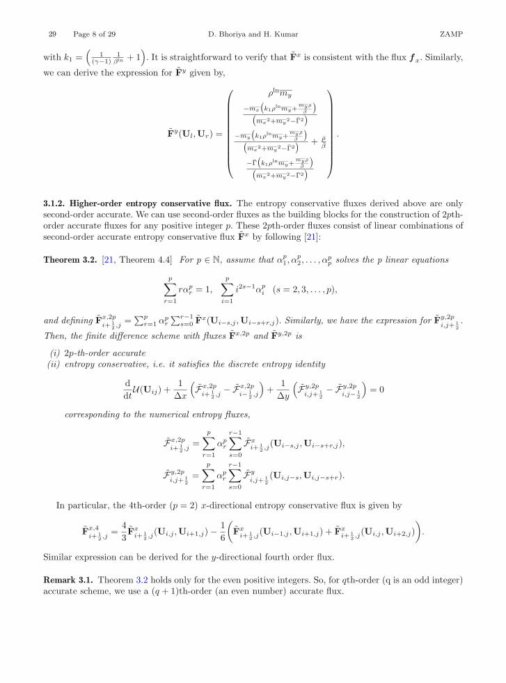
3.1.2. Higher-order entropy conservative flux. The entropy conservative fluxes derived above are onlysecond-order accurate. We can use second-order fluxes as the building blocks for the construction of 2pth-order accurate fluxes for any positive integer p. These 2pth-order fluxes consist of linear combinations ofsecond-order accurate entropy conservative flux Fx by following [21]:
Theorem 3.2. [21, Theorem 4.4] For p ∈ N, assume that αp1, α
p2, . . . , α
pp solves the p linear equations
p∑r=1
rαpr = 1,
p∑i=1
i2s−1αpi (s = 2, 3, . . . , p),
and defining Fx,2p
i+ 12 ,j
=∑p
r=1 αpr
∑r−1s=0 F
x(Ui−s,j ,Ui−s+r,j). Similarly, we have the expression for Fy,2p
i,j+ 12.
Then, the finite difference scheme with fluxes Fx,2p and Fy,2p is
(i) 2p-th-order accurate(ii) entropy conservative, i.e. it satisfies the discrete entropy identity
ddt
U(Uij) +1
Δx
(Fx,2p
i+ 12 ,j
− Fx,2p
i− 12 ,j
)+
1Δy
(Fy,2p
i,j+ 12
− Fy,2p
i,j− 12
)= 0
corresponding to the numerical entropy fluxes,
Fx,2p
i+ 12 ,j
=p∑
r=1
αpr
r−1∑s=0
Fxi+ 1
2 ,j(Ui−s,j ,Ui−s+r,j),
Fy,2p
i,j+ 12
=p∑
r=1
αpr
r−1∑s=0
Fy
i,j+ 12(Ui,j−s,Ui,j−s+r).
In particular, the 4th-order (p = 2) x-directional entropy conservative flux is given by
Fx,4
i+ 12 ,j
=43Fx
i+ 12 ,j(Ui,j ,Ui+1,j) − 1
6
(Fx
i+ 12 ,j(Ui−1,j ,Ui+1,j) + Fx
i+ 12 ,j(Ui,j ,Ui+2,j)
).
Similar expression can be derived for the y-directional fourth order flux.
Remark 3.1. Theorem 3.2 holds only for the even positive integers. So, for qth-order (q is an odd integer)accurate scheme, we use a (q + 1)th-order (an even number) accurate flux.

ZAMP Entropy-stable schemes for relativistic hydrodynamics equations Page 9 of 29 29
3.2. Entropy-stable schemes
The entropy conservative schemes will produce high-frequency oscillations near the shocks as they do notdissipate entropy at the shocks. We follow [34] to introduce modified fluxes which will ensure entropystability at the shocks. We consider
Fxi+ 1
2 ,j = Fxi+ 1
2 ,j − 12Dx
i+ 12 ,j�v�i+ 1
2 ,j ,
Fy
i,j+ 12
= Fy
i,j+ 12
− 12Dy
i,j+ 12�v�i,j+ 1
2,
(22)
where Dxi+ 1
2 ,j and Dy
i,j+ 12
are symmetric positive definite matrices. Then, we have the following lemma:
Lemma 3.3. [34] The numerical scheme (20) with the modified numerical fluxes (22) is entropy stable,i.e. the computed solution satisfies
ddt
U(Uij) +1
Δx
(Fx
i+ 12 ,j − Fx
i− 12 ,j
)+
1Δy
(Fy
i,j+ 12
− Fy
i,j− 12
)≤ 0
with the consistent numerical entropy flux functions,
Fxi+ 1
2 ,j = Fxi+ 1
2 ,j +12v�
i+ 12 ,jD
xi+ 1
2 ,j�v�i+ 12 ,j and Fy
i,j+ 12
= Fy
i,j+ 12
+12v�
i,j+ 12Dy
i,j+ 12�v�i,j+ 1
2.
Here, we use Rusanov’s type diffusion operators for the matrix D given by,
Dxi+ 1
2 ,j = Rxi+ 1
2 ,jΛxi+ 1
2 ,jRx�i+ 1
2 ,j , and Dy
i,j+ 12
= Ry
i,j+ 12Λy
i,j+ 12Ry�
i,j+ 12
(23)
where Ri, i ∈ {x, y}, are matrices of the entropy scaled right eigenvectors (see Appendix B) of theJacobian ∂f i
∂U , and Λi, i ∈ {x, y}, are 4 × 4 diagonal matrices of the form
Λi = diag{(
max1≤k≤4
|λik|)I4×4
}, i ∈ {x, y},
where {λik : 1 ≤ k ≤ 4} is the set of eigenvalue of the Jacobian ∂f i
∂U . We also note that, following [4],Uv = Rk(Rk)� for k ∈ {x, y} and hence,
RkΛk(Rk)(−1)�U� ≈ RkΛk(Rk)(−1)Uv�v� = RkΛk(Rk)��v�.
Hence, the entropy diffusion operator used here is similar to the Roe diffusion operator, when the entropyscaled right eigenvectors are used.
With the choice of diffusion operator (23), the numerical scheme (20) with the numerical flux (22) isentropy stable. However, the scheme is only first-order accurate due to the presence of the jump terms�v�i+ 1
2 ,j and �v�i,j+ 12.
3.3. High-order diffusion operators
A straightforward way to increase the order of accuracy is to approximate the jumps using higher-orderreconstruction process. However, proving the entropy stability of the resulting scheme is not possible.Instead, we follow the process prescribed in [12] and introduce the scaled entropy variables,
Wx,±ij = Rx�
i± 12 ,jvij .
If Wx,±ij denotes the k-th-order reconstructed values of Wx,±
i,j in the x-direction, then,
px,±ij =
{Rx�
i± 12 ,j
}(−1)
Wx,±i,j ,

29 Page 10 of 29 D. Bhoriya and H. Kumar ZAMP
Table 1. Coefficients for Runge–Kutta time stepping
Order αil βil
2 1 1
1/2 1/2 0 1/23 1 1
3/4 1/4 0 1/41/3 0 2/3 0 0 2/3
are the corresponding k-th-order reconstructed values for vij . Hence, the modified numerical flux is givenby,
Fx,k
i+ 12 ,j
= Fx,2p
i+ 12 ,j − 1
2Dx
i+ 12 ,j�P
x�i+ 12 ,j (24)
where �Px�i+ 12 ,j stands for,
�Px�i+ 12 ,j = Px,−
i+1,j − Px,+ij ,
and p ∈ N is chosen as• p = k/2 if k is even,• p = (k + 1)/2 if k is odd.
Following [12], a sufficient condition for the numerical flux (24) to be entropy stable is that the recon-struction process for W must satisfy the sign-preserving property. For the second-order reconstruction,we use the minmod reconstruction which satisfies this property. We denote this scheme by O2-ES. Forthe higher-order scheme, we follow [13] and use the ENO reconstruction. We use third- and fourth-orderENO-based reconstruction and denote these schemes by O3-ES and O4-ES, respectively.
3.4. Semi-discrete entropy stability
We now have the following result:
Theorem 3.4. The semi-discrete schemes O2-ES, O3-ES and O4-ES designed above are entropy stable,i.e. they satisfy,
ddt
U(Uij) +1
Δx
(Fx
i+ 12 ,j − Fx
i− 12 ,j
)+
1Δy
(Fy
i,j+ 12
− Fy
i,j− 12
)≤ 0
where Fx and Fy are the consistent numerical entropy fluxes.
3.5. Time discretization
For the time discretization, we use SSP Runge–Kutta methods [16]. The second- and third-order accurateSSP-RK methods rely on the following algorithm:
1. Define U0 = Un.2. For m = 1, . . . , k + 1, evaluate,
U(m)i,j =
m−1∑l=0
αmlU(l)i,j + βmlΔtn(Li,j(U(l))),
where, αml and βml follows from Table 1.3. Set Un+1
i,j = U(k+1)i,j .

ZAMP Entropy-stable schemes for relativistic hydrodynamics equations Page 11 of 29 29
Table 2. Accuracy test: rate of convergence of second-order (O2-ES), third-order (O3-ES) and fourth-order (O4-ES)entropy-stable schemes
Number of cells O2-ES O3-ES O4-ES
– L1 error Order L1 error Order L1 error Order
100 1.4397E−02 – 1.2232E−04 – 1.1444E−05 –
200 3.9752E−03 1.86 1.5290E−05 3.00 8.1805E−07 3.81400 1.0807E−03 1.88 1.9115E−06 2.99 5.7077E−08 3.84800 2.9050E−04 1.89 2.3896E−07 2.99 3.8740E−09 3.881600 7.6511E−05 1.92 2.9871E−08 2.99 2.5967E−10 3.90
For the fourth-order accuracy, we consider the following time update:
U1 = Un + 0.39175222700392(ΔtL(Un)),
U2 = 0.44437049406734(Un) + 0.55562950593266(U1) + 0.36841059262959(ΔtL(U1)),
U3 = 0.62010185138540(Un) + 0.37989814861460(U2) + 0.25189177424738(ΔtL(U2)),
U4 = 0.17807995410773(Un) + 0.82192004589227(U3) + 0.54497475021237(ΔtL(U3)),
and finally,
Un+1 = 0.00683325884039(Un) + 0.51723167208978(U2) + 0.12759831133288(U3)
+0.34833675773694(U4) + 0.08460416338212(ΔtL(U3)) + 0.22600748319395(ΔtL(U4)).
4. Numerical results
We will now present numerical test cases for the above schemes. We present both one- and two-dimensionaltest cases and compute several Riemann problems. We use CFL number 0.2 for all the presented testcases.
4.1. One-dimensional test cases
4.1.1. Accuracy test. To test the accuracy of the proposed schemes, we first consider a problem which hassmooth solution. We consider the computational domain [0, 1] with periodic boundary conditions. Theinitial density profile is assumed to be ρ(x, 0) = 2 + sin(2πx), which is then advected with the velocityu = (0.5, 0)�. The pressure is assumed to be constant with p = 1.0. The exact solution is transportationof the density profile in x-direction, i.e. ρ(x, t) = 2 + sin(2π(x − t)), while the other variables remainunchanged. We use the adiabatic index, γ = 5
3 . The simulations are performed till time t = 2.0.We present L1-errors of the density profile for the O2-ES, O3-ES, and O4-ES schemes at 100, 200,
400, 800 and 1600 cells in Table 2. We note that all the schemes preserve the predicted order of accuracy.
4.1.2. Isentropic smooth flows. In this test case, we consider a one-dimensional isentropic smooth pulsein a fixed reference state, wref = (ρref ,uref , pref ). A detailed illustration of the problem is given in [23]and [40]. We set ρref = 1, uref = 0, pref = 100. For the initial pulse we consider α = 1 and L = 0.3 andthen set the density profile as,
ρ0(x) = ρref [1 + αf(x)],where f is given by
f(x) =
⎧⎨⎩
[(xL
)2 − 1]4
, if |x| < L
0, otherwise.
29 Page 12 of 29 D. Bhoriya and H. Kumar ZAMP
0.8
1
1.2
1.4
1.6
1.8
2
2.2
Exact solutionO2-ES on 80 cellsO3-ES on 80 cellsO4-ES on 80 cells
(a) Density
-0.1
0
0.1
0.2
0.3
0.4
0.5
0.6
Exact solutionO2-ES on 80 cellsO3-ES on 80 cellsO4-ES on 80 cells
(b) Velocity
50
100
150
200
250
300
350
Exact solutionO2-ES on 80 cellsO3-ES on 80 cellsO4-ES on 80 cells
(c) Pressure
-0.4 -0.2 0 0.2 0.4 0.6 0.8 1 -0.4 -0.2 0 0.2 0.4 0.6 0.8 1
-0.4 -0.2 0 0.2 0.4 0.6 0.8 1 0 0.1 0.2 0.3 0.4 0.5 0.6 0.7 0.8
Time
-295
-294.8
-294.6
-294.4
-294.2
-294
-293.8
-293.6
-293.4
-293.2
-293
Ent
ropy
O2-ES on 80 cellsO3-ES on 80 cellsO4-ES on 80 cells
(d) Total Entropy evolution with time
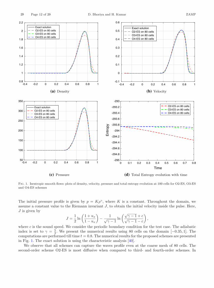
Fig. 1. Isentropic smooth flows: plots of density, velocity, pressure and total entropy evolution at 100 cells for O2-ES, O3-ESand O4-ES schemes
The initial pressure profile is given by p = Kργ , where K is a constant. Throughout the domain, weassume a constant value to the Riemann invariant J , to obtain the initial velocity inside the pulse. Here,J is given by
J =12
ln(
1 + ux
1 − ux
)− 1√
γ − 1ln(√
γ − 1 + c√γ − 1 − c
),
where c is the sound speed. We consider the periodic boundary condition for the test case. The adiabaticindex is set to γ = 5
3 . We present the numerical results using 80 cells on the domain [−0.35, 1]. Thecomputations are performed till time t = 0.8. The numerical results for the proposed schemes are presentedin Fig. 1. The exact solution is using the characteristic analysis [40].
We observe that all schemes can capture the waves profile even at the coarse mesh of 80 cells. Thesecond-order scheme O2-ES is most diffusive when compared to third- and fourth-order schemes. In
ZAMP Entropy-stable schemes for relativistic hydrodynamics equations Page 13 of 29 29
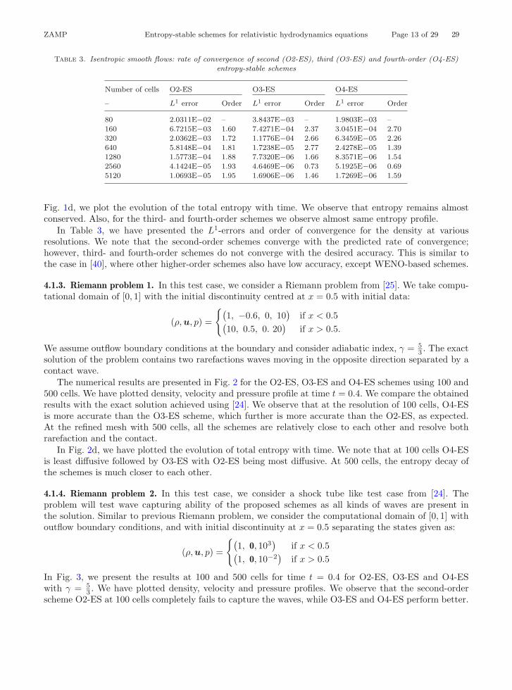
Table 3. Isentropic smooth flows: rate of convergence of second (O2-ES), third (O3-ES) and fourth-order (O4-ES)entropy-stable schemes
Number of cells O2-ES O3-ES O4-ES
– L1 error Order L1 error Order L1 error Order
80 2.0311E−02 – 3.8437E−03 – 1.9803E−03 –
160 6.7215E−03 1.60 7.4271E−04 2.37 3.0451E−04 2.70320 2.0362E−03 1.72 1.1776E−04 2.66 6.3459E−05 2.26640 5.8148E−04 1.81 1.7238E−05 2.77 2.4278E−05 1.39
1280 1.5773E−04 1.88 7.7320E−06 1.66 8.3571E−06 1.542560 4.1424E−05 1.93 4.6469E−06 0.73 5.1925E−06 0.695120 1.0693E−05 1.95 1.6906E−06 1.46 1.7269E−06 1.59
Fig. 1d, we plot the evolution of the total entropy with time. We observe that entropy remains almostconserved. Also, for the third- and fourth-order schemes we observe almost same entropy profile.
In Table 3, we have presented the L1-errors and order of convergence for the density at variousresolutions. We note that the second-order schemes converge with the predicted rate of convergence;however, third- and fourth-order schemes do not converge with the desired accuracy. This is similar tothe case in [40], where other higher-order schemes also have low accuracy, except WENO-based schemes.
4.1.3. Riemann problem 1. In this test case, we consider a Riemann problem from [25]. We take compu-tational domain of [0, 1] with the initial discontinuity centred at x = 0.5 with initial data:
(ρ,u, p) =
{(1, −0.6, 0, 10
)if x < 0.5(
10, 0.5, 0. 20)
if x > 0.5.
We assume outflow boundary conditions at the boundary and consider adiabatic index, γ = 53 . The exact
solution of the problem contains two rarefactions waves moving in the opposite direction separated by acontact wave.
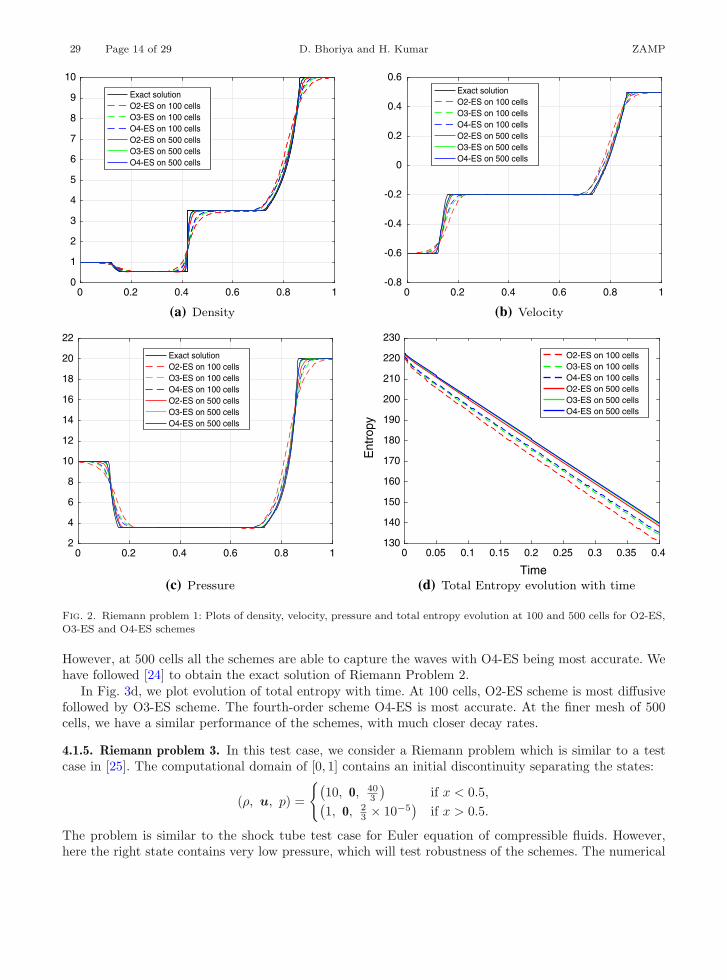
The numerical results are presented in Fig. 2 for the O2-ES, O3-ES and O4-ES schemes using 100 and500 cells. We have plotted density, velocity and pressure profile at time t = 0.4. We compare the obtainedresults with the exact solution achieved using [24]. We observe that at the resolution of 100 cells, O4-ESis more accurate than the O3-ES scheme, which further is more accurate than the O2-ES, as expected.At the refined mesh with 500 cells, all the schemes are relatively close to each other and resolve bothrarefaction and the contact.
In Fig. 2d, we have plotted the evolution of total entropy with time. We note that at 100 cells O4-ESis least diffusive followed by O3-ES with O2-ES being most diffusive. At 500 cells, the entropy decay ofthe schemes is much closer to each other.
4.1.4. Riemann problem 2. In this test case, we consider a shock tube like test case from [24]. Theproblem will test wave capturing ability of the proposed schemes as all kinds of waves are present inthe solution. Similar to previous Riemann problem, we consider the computational domain of [0, 1] withoutflow boundary conditions, and with initial discontinuity at x = 0.5 separating the states given as:
(ρ,u, p) =
{(1, 0, 103
)if x < 0.5(
1, 0, 10−2)
if x > 0.5
In Fig. 3, we present the results at 100 and 500 cells for time t = 0.4 for O2-ES, O3-ES and O4-ESwith γ = 5
3 . We have plotted density, velocity and pressure profiles. We observe that the second-orderscheme O2-ES at 100 cells completely fails to capture the waves, while O3-ES and O4-ES perform better.
29 Page 14 of 29 D. Bhoriya and H. Kumar ZAMP
0
1
2
3
4
5
6
7
8
9
10
Exact solutionO2-ES on 100 cellsO3-ES on 100 cellsO4-ES on 100 cellsO2-ES on 500 cellsO3-ES on 500 cellsO4-ES on 500 cells
(a) Density
-0.8
-0.6
-0.4
-0.2
0
0.2
0.4
0.6Exact solutionO2-ES on 100 cellsO3-ES on 100 cellsO4-ES on 100 cellsO2-ES on 500 cellsO3-ES on 500 cellsO4-ES on 500 cells
(b) Velocity
2
4
6
8
10
12
14
16
18
20
22
Exact solutionO2-ES on 100 cellsO3-ES on 100 cellsO4-ES on 100 cellsO2-ES on 500 cellsO3-ES on 500 cellsO4-ES on 500 cells
(c) Pressure
0 0.2 0.4 0.6 0.8 1 0 0.2 0.4 0.6 0.8 1
0 0.2 0.4 0.6 0.8 1 0 0.05 0.1 0.15 0.2 0.25 0.3 0.35 0.4
Time
130
140
150
160
170
180
190
200
210
220
230
Ent
ropy
O2-ES on 100 cellsO3-ES on 100 cellsO4-ES on 100 cellsO2-ES on 500 cellsO3-ES on 500 cellsO4-ES on 500 cells
(d) Total Entropy evolution with time
Fig. 2. Riemann problem 1: Plots of density, velocity, pressure and total entropy evolution at 100 and 500 cells for O2-ES,O3-ES and O4-ES schemes
However, at 500 cells all the schemes are able to capture the waves with O4-ES being most accurate. Wehave followed [24] to obtain the exact solution of Riemann Problem 2.
In Fig. 3d, we plot evolution of total entropy with time. At 100 cells, O2-ES scheme is most diffusivefollowed by O3-ES scheme. The fourth-order scheme O4-ES is most accurate. At the finer mesh of 500cells, we have a similar performance of the schemes, with much closer decay rates.
4.1.5. Riemann problem 3. In this test case, we consider a Riemann problem which is similar to a testcase in [25]. The computational domain of [0, 1] contains an initial discontinuity separating the states:
(ρ, u, p) =
{(10, 0, 40
3
)if x < 0.5,(
1, 0, 23 × 10−5
)if x > 0.5.
The problem is similar to the shock tube test case for Euler equation of compressible fluids. However,here the right state contains very low pressure, which will test robustness of the schemes. The numerical

ZAMP Entropy-stable schemes for relativistic hydrodynamics equations Page 15 of 29 29
0
2
4
6
8
10
12Exact solutionO2-ES on 100 cellsO3-ES on 100 cellsO4-ES on 100 cellsO2-ES on 500 cellsO3-ES on 500 cellsO4-ES on 500 cells
(a) Density
0
0.1
0.2
0.3
0.4
0.5
0.6
0.7
0.8
0.9
1
Exact solutionO2-ES on 100 cellsO3-ES on 100 cellsO4-ES on 100 cellsO2-ES on 500 cellsO3-ES on 500 cellsO4-ES on 500 cells
(b) Velocity
0
100
200
300
400
500
600
700
800
900
1000Exact solutionO2-ES on 100 cellsO3-ES on 100 cellsO4-ES on 100 cellsO2-ES on 500 cellsO3-ES on 500 cellsO4-ES on 500 cells
(c) Pressure
0 0.2 0.4 0.6 0.8 1 0 0.2 0.4 0.6 0.8 1
0 0.2 0.4 0.6 0.8 1 0 0.05 0.1 0.15 0.2 0.25 0.3 0.35 0.4
Time
-240
-220
-200
-180
-160
-140
-120
-100
-80
-60
Ent
ropy
O2-ES on 100 cellsO3-ES on 100 cellsO4-ES on 100 cellsO2-ES on 500 cellsO3-ES on 500 cellsO4-ES on 500 cells
(d) Total Entropy evolution with time
Fig. 3. Riemann problem 2: Plots of density, velocity, pressure and total entropy evolution at 100 and 500 cells for O2-ES,O3-ES and O4-ES schemes
results are presented in Fig. 4 at time t = 0.4. We use adiabatic index, γ = 53 . We proceed as in [24] to
obtain the exact solution of Riemann Problem 3. Similar to test case above, at 100 cells, no scheme isable to capture the shock wave efficiently. However, at 500 cells, all the schemes resolve the shock wavewith accuracy. For the entropy evolution, we observe that at 500 cells all the scheme have similar decayrate, whereas for the 100 cells, O3-ES and O4-ES are slightly better than the O2-ES.
4.1.6. Density perturbation test case. For this test case, we consider the test problem from [38]. Weconsider the computational domain of [0, 1] with outflow boundary conditions. We assume adiabaticindex to be γ = 5
3 . The initial conditions are given by,
(ρ,u, p) =
{(5, 0, 50
)if x < 0.5(
2 + 0.3 sin(50x), 0, 5)
if x > 0.5.

29 Page 16 of 29 D. Bhoriya and H. Kumar ZAMP
0
1
2
3
4
5
6
7
8
9
10
11
Exact solutionO2-ES on 100 cellsO3-ES on 100 cellsO4-ES on 100 cellsO2-ES on 500 cellsO3-ES on 500 cellsO4-ES on 500 cells
(a) Density
-0.1
0
0.1
0.2
0.3
0.4
0.5
0.6
0.7
0.8
Exact solutionO2-ES on 100 cellsO3-ES on 100 cellsO4-ES on 100 cellsO2-ES on 500 cellsO3-ES on 500 cellsO4-ES on 500 cells
(b) Velocity
0
2
4
6
8
10
12
14
Exact solutionO2-ES on 100 cellsO3-ES on 100 cellsO4-ES on 100 cellsO2-ES on 500 cellsO3-ES on 500 cellsO4-ES on 500 cells
(c) Pressure
0 0.2 0.4 0.6 0.8 1 0 0.2 0.4 0.6 0.8 1
0 0.2 0.4 0.6 0.8 1 0 0.05 0.1 0.15 0.2 0.25 0.3 0.35 0.4
Time
550
600
650
700
750
800
Ent
ropy
O2-ES on 100 cellsO3-ES on 100 cellsO4-ES on 100 cellsO2-ES on 500 cellsO3-ES on 500 cellsO4-ES on 500 cells
(d) Total Entropy evolution with time
Fig. 4. Riemann problem 3: plots of density, velocity, pressure and total entropy evolution at 100 and 500 cells for O2-ES,O3-ES and O4-ES schemes
The solution is computed till time t = 0.35. The exact solution of the problem contains oscillatory densityprofile with both shocks and rarefaction waves. Hence, the problem will test accuracy of the schemes incapturing these oscillations and other waves.
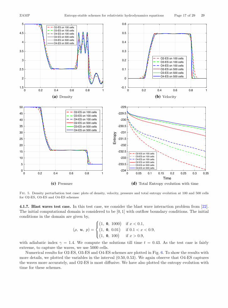
We have plotted the numerical results for density, velocity and pressure in Fig. 5 for 100 and 500cells using O2-ES, O3-ES, and O4-ES schemes. At coarse mesh of 100 cells, we again observe that thefourth-order scheme O4-ES is much more accurate than the third-order scheme O3-ES. The second-orderscheme is the least accurate. For the fine mesh of 500 cells, O2-ES still fails to capture the peaks; however,O3-ES and O4-ES perform almost identically. This can be further observed from the entropy decay plotin Fig. 5d. We observe that the O3-ES and O4-ES schemes are much closer for 500 cells with O2-ESbeing more diffusive.
ZAMP Entropy-stable schemes for relativistic hydrodynamics equations Page 17 of 29 29
1.5
2
2.5
3
3.5
4
4.5
5O2-ES on 100 cellsO3-ES on 100 cellsO4-ES on 100 cellsO2-ES on 500 cellsO3-ES on 500 cellsO4-ES on 500 cells
(a) Density
-0.1
0
0.1
0.2
0.3
0.4
0.5
0.6
O2-ES on 100 cellsO3-ES on 100 cellsO4-ES on 100 cellsO2-ES on 500 cellsO3-ES on 500 cellsO4-ES on 500 cells
(b) Velocity
0
5
10
15
20
25
30
35
40
45
50
O2-ES on 100 cellsO3-ES on 100 cellsO4-ES on 100 cellsO2-ES on 500 cellsO3-ES on 500 cellsO4-ES on 500 cells
(c) Pressure
0 0.2 0.4 0.6 0.8 1 0 0.2 0.4 0.6 0.8 1
0 0.2 0.4 0.6 0.8 1 0 0.05 0.1 0.15 0.2 0.25 0.3 0.35
Time
-234
-233.5
-233
-232.5
-232
-231.5
-231
-230.5
-230
-229.5
-229
Ent
ropy
O2-ES on 100 cellsO3-ES on 100 cellsO4-ES on 100 cellsO2-ES on 500 cellsO3-ES on 500 cellsO4-ES on 500 cells
(d) Total Entropy evolution with time
Fig. 5. Density perturbation test case: plots of density, velocity, pressure and total entropy evolution at 100 and 500 cellsfor O2-ES, O3-ES and O4-ES schemes
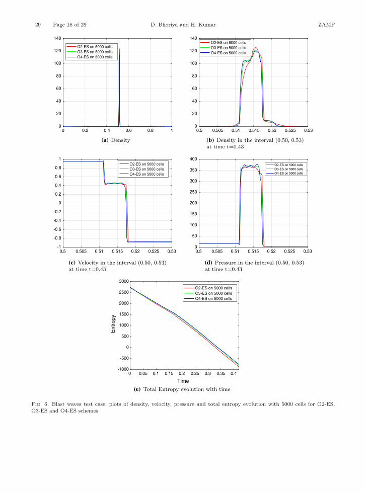
4.1.7. Blast waves test case. In this test case, we consider the blast wave interaction problem from [22].The initial computational domain is considered to be [0, 1] with outflow boundary conditions. The initialconditions in the domain are given by,
(ρ, u, p) =
⎧⎪⎨⎪⎩
(1, 0, 1000
)if x < 0.1,(
1, 0, 0.01)
if 0.1 < x < 0.9,(1, 0, 100
)if x > 0.9,
with adiabatic index γ = 1.4. We compute the solutions till time t = 0.43. As the test case is fairlyextreme, to capture the waves, we use 5000 cells.
Numerical results for O2-ES, O3-ES and O4-ES schemes are plotted in Fig. 6. To show the results withmore details, we plotted the variables in the interval (0.50, 0.53). We again observe that O4-ES capturesthe waves more accurately, and O2-ES is most diffusive. We have also plotted the entropy evolution withtime for these schemes.
29 Page 18 of 29 D. Bhoriya and H. Kumar ZAMP
0
20
40
60
80
100
120
140
O2-ES on 5000 cellsO3-ES on 5000 cellsO4-ES on 5000 cells
(a) Density
0
20
40
60
80
100
120
140O2-ES on 5000 cellsO3-ES on 5000 cellsO4-ES on 5000 cells
(b) Density in the interval (0.50, 0.53)at time t=0.43
-1
-0.8
-0.6
-0.4
-0.2
0
0.2
0.4
0.6
0.8
1O2-ES on 5000 cellsO3-ES on 5000 cellsO4-ES on 5000 cells
(c) Velocity in the interval (0.50, 0.53)at time t=0.43
0
50
100
150
200
250
300
350
400O2-ES on 5000 cellsO3-ES on 5000 cellsO4-ES on 5000 cells
(d) Pressure in the interval (0.50, 0.53)at time t=0.43
0 0.2 0.4 0.6 0.8 1 0.5 0.505 0.51 0.515 0.52 0.525 0.53
0.5 0.505 0.51 0.515 0.52 0.525 0.53 0.5 0.505 0.51 0.515 0.52 0.525 0.53
0 0.05 0.1 0.15 0.2 0.25 0.3 0.35 0.4
Time
-1000
-500
0
500
1000
1500
2000
2500
3000
Ent
ropy
O2-ES on 5000 cellsO3-ES on 5000 cellsO4-ES on 5000 cells
(e) Total Entropy evolution with time
Fig. 6. Blast waves test case: plots of density, velocity, pressure and total entropy evolution with 5000 cells for O2-ES,
O3-ES and O4-ES schemes

ZAMP Entropy-stable schemes for relativistic hydrodynamics equations Page 19 of 29 29
0 0.2 0.4 0.6 0.8 10
0.1
0.2
0.3
0.4
0.5
0.6
0.7
0.8
0.9
1
(a) ln ρ using O3-ES
0 0.2 0.4 0.6 0.8 10
0.1
0.2
0.3
0.4
0.5
0.6
0.7
0.8
0.9
1
(b) ln ρ using O4-ES
0 0.2 0.4 0.6 0.8 10
0.1
0.2
0.3
0.4
0.5
0.6
0.7
0.8
0.9
1
(c) ln p using O3-ES
0 0.2 0.4 0.6 0.8 10
0.1
0.2
0.3
0.4
0.5
0.6
0.7
0.8
0.9
1
(d) ln p using O4-ES
Fig. 7. Two-dimensional Riemann problem 1: plots for ln ρ and ln p for O3-ES and O4-ES using 25 contours
4.2. Two-dimensional test cases
For the two-dimensional test cases, we consider various two-dimensional Riemann problems. We assumea computational domain [0, 1]× [0, 1] which is divided into four parts with initial discontinuities along thelines x = 0.5 and y = 0.5. We use mesh of 400 × 400 cells and take γ = 5
3 . Outflow boundary conditionsare used in all the test cases. To simplify the presentation, we present the numerical results for O3-ESand O4-ES schemes only, as O2-ES numerical results are more diffusion compare to O3-ES and O4-ESschemes.
29 Page 20 of 29 D. Bhoriya and H. Kumar ZAMP
0 0.2 0.4 0.6 0.8 10
0.1
0.2
0.3
0.4
0.5
0.6
0.7
0.8
0.9
1
(a) ln ρ using O3-ES0 0.2 0.4 0.6 0.8 1
0
0.1
0.2
0.3
0.4
0.5
0.6
0.7
0.8
0.9
1
(b) ln ρ using O4-ES
0 0.2 0.4 0.6 0.8 10
0.1
0.2
0.3
0.4
0.5
0.6
0.7
0.8
0.9
1
(c) ln p using O3-ES
0 0.2 0.4 0.6 0.8 10
0.1
0.2
0.3
0.4
0.5
0.6
0.7
0.8
0.9
1
(d) ln p using O4-ES
Fig. 8. Two-dimensional Riemann problem 2: plots for ln ρ and ln p for O3-ES and O4-ES using 25 contours
4.2.1. Two-dimensional Riemann problem 1. In this test case, we consider the Riemann problem from[38]. The domain is filled with four constant states given by,
(ρ, ux, uy, p) =
⎧⎪⎪⎪⎨⎪⎪⎪⎩
(0.1, 0, 0, 0.01
), for x, y > 0.5,(
0.1, 0.99, 0, 1.0), for x < 0.5, y > 0.5,(
0.5, 0, 0, 1.0), for x, y < 0.5,(
0.1, 0, 0.99, 1.0), for x > 0.5, y < 0.5.

ZAMP Entropy-stable schemes for relativistic hydrodynamics equations Page 21 of 29 29
0 0.2 0.4 0.6 0.8 10
0.1
0.2
0.3
0.4
0.5
0.6
0.7
0.8
0.9
1
(a) ln ρ using O3-ES
0 0.2 0.4 0.6 0.8 10
0.1
0.2
0.3
0.4
0.5
0.6
0.7
0.8
0.9
1
(b) ln ρ using O4-ES
0 0.2 0.4 0.6 0.8 10
0.1
0.2
0.3
0.4
0.5
0.6
0.7
0.8
0.9
1
(c) ln p using O3-ES
0 0.2 0.4 0.6 0.8 10
0.1
0.2
0.3
0.4
0.5
0.6
0.7
0.8
0.9
1
(d) ln p using O4-ES
Fig. 9. Two-dimensional Riemann problem 3: plots for ln ρ and ln p for O3-ES and O4-ES using 25 contours
Numerical results for O3-ES and O4-ES schemes are presented in Fig. 7 at time t = 0.4. We haveplotted 25 contours of ln ρ and ln p. We note that both the schemes captures all the waves and havecomparable accuracy with O4-ES being slightly more accurate.
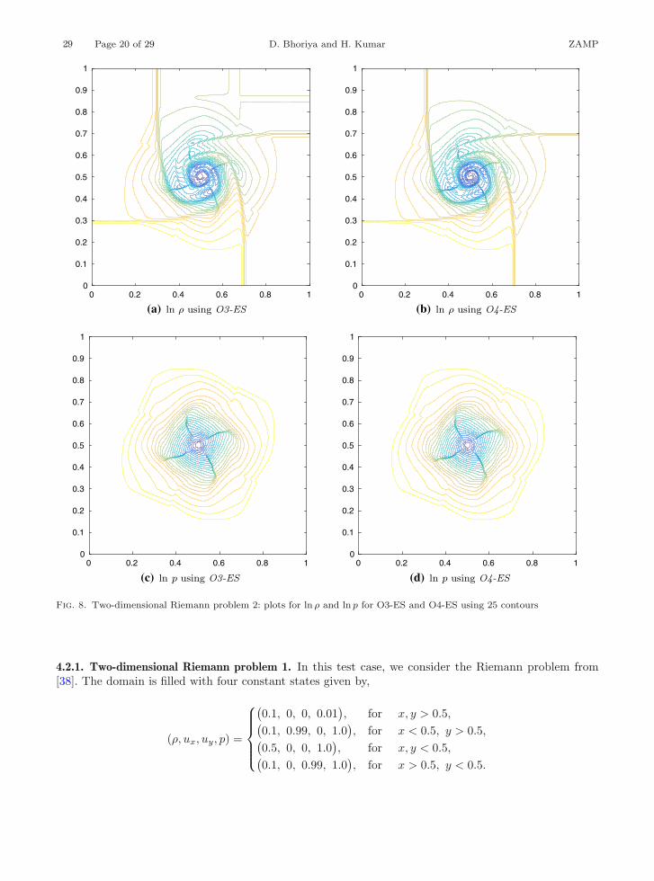
4.2.2. Two-dimensional Riemann problem 2. For this test case, we consider a Riemann problem used in[28]. The four initial states are given by,

29 Page 22 of 29 D. Bhoriya and H. Kumar ZAMP
0 0.2 0.4 0.6 0.8 10
0.1
0.2
0.3
0.4
0.5
0.6
0.7
0.8
0.9
1
(a) ln ρ using O3-ES
0 0.2 0.4 0.6 0.8 10
0.1
0.2
0.3
0.4
0.5
0.6
0.7
0.8
0.9
1
(b) ln ρ using O4-ES
0 0.2 0.4 0.6 0.8 10
0.1
0.2
0.3
0.4
0.5
0.6
0.7
0.8
0.9
1
(c) ln p using O3-ES
0 0.2 0.4 0.6 0.8 10
0.1
0.2
0.3
0.4
0.5
0.6
0.7
0.8
0.9
1
(d) ln p using O4-ES
Fig. 10. Two-dimensional Riemann problem 4: plots for ln ρ and ln p for O3-ES and O4-ES using 25 contours
(ρ,u, p) =
⎧⎪⎪⎪⎨⎪⎪⎪⎩
(0.5, 0.5, −0.5, 5
), if x, y > 0.5,(
1, 0.5, 0.5, 5), if x < 0.5, y > 0.5,(
3, −0.5, 0.5, 5), if x, y < 0.5,(
1.5, −0.5, −0.5, 5), if x > 0.5, y < 0.5.
In Fig. 8, we have plotted ln ρ and ln p using 25 contours at t = 0.4 for O3-ES and O4-ES schemes.We again observe that both the schemes accurately capture all the waves in the vortex. Also, O4-ESproduces more details compared to O3-ES.
ZAMP Entropy-stable schemes for relativistic hydrodynamics equations Page 23 of 29 29
0 0.2 0.4 0.6 0.8 10
0.1
0.2
0.3
0.4
0.5
0.6
0.7
0.8
0.9
1
(a) ln ρ using O3-ES
0 0.2 0.4 0.6 0.8 10
0.1
0.2
0.3
0.4
0.5
0.6
0.7
0.8
0.9
1
(b) ln ρ using O4-ES
0 0.2 0.4 0.6 0.8 10
0.1
0.2
0.3
0.4
0.5
0.6
0.7
0.8
0.9
1
(c) ln p using O3-ES
0 0.2 0.4 0.6 0.8 10
0.1
0.2
0.3
0.4
0.5
0.6
0.7
0.8
0.9
1
(d) ln p using O4-ES
Fig. 11. Two-dimensional Riemann problem 5: plots for ln ρ and ln p for O3-ES and O4-ES using 25 contours
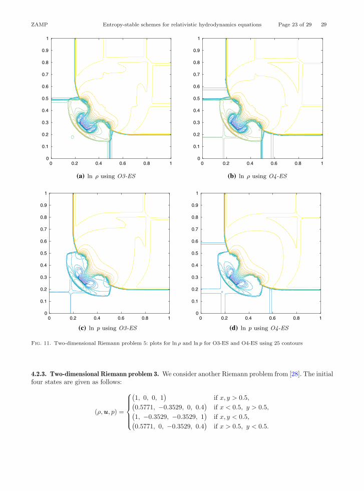
4.2.3. Two-dimensional Riemann problem 3. We consider another Riemann problem from [28]. The initialfour states are given as follows:
(ρ,u, p) =
⎧⎪⎪⎪⎨⎪⎪⎪⎩
(1, 0, 0, 1
)if x, y > 0.5,(
0.5771, −0.3529, 0, 0.4)
if x < 0.5, y > 0.5,(1, −0.3529, −0.3529, 1
)if x, y < 0.5,(
0.5771, 0, −0.3529, 0.4)
if x > 0.5, y < 0.5.
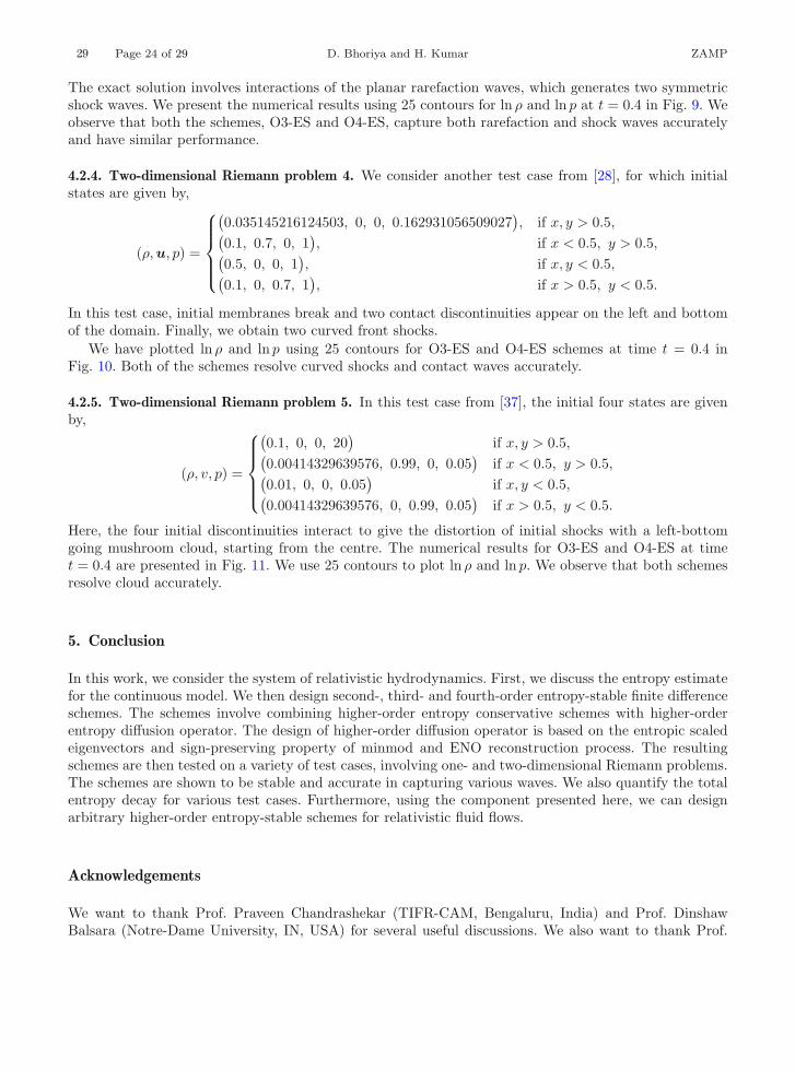
29 Page 24 of 29 D. Bhoriya and H. Kumar ZAMP
The exact solution involves interactions of the planar rarefaction waves, which generates two symmetricshock waves. We present the numerical results using 25 contours for ln ρ and ln p at t = 0.4 in Fig. 9. Weobserve that both the schemes, O3-ES and O4-ES, capture both rarefaction and shock waves accuratelyand have similar performance.
4.2.4. Two-dimensional Riemann problem 4. We consider another test case from [28], for which initialstates are given by,
(ρ,u, p) =
⎧⎪⎪⎪⎨⎪⎪⎪⎩
(0.035145216124503, 0, 0, 0.162931056509027
), if x, y > 0.5,(
0.1, 0.7, 0, 1), if x < 0.5, y > 0.5,(
0.5, 0, 0, 1), if x, y < 0.5,(
0.1, 0, 0.7, 1), if x > 0.5, y < 0.5.
In this test case, initial membranes break and two contact discontinuities appear on the left and bottomof the domain. Finally, we obtain two curved front shocks.
We have plotted ln ρ and ln p using 25 contours for O3-ES and O4-ES schemes at time t = 0.4 inFig. 10. Both of the schemes resolve curved shocks and contact waves accurately.
4.2.5. Two-dimensional Riemann problem 5. In this test case from [37], the initial four states are givenby,
(ρ, v, p) =
⎧⎪⎪⎪⎨⎪⎪⎪⎩
(0.1, 0, 0, 20
)if x, y > 0.5,(
0.00414329639576, 0.99, 0, 0.05)
if x < 0.5, y > 0.5,(0.01, 0, 0, 0.05
)if x, y < 0.5,(
0.00414329639576, 0, 0.99, 0.05)
if x > 0.5, y < 0.5.
Here, the four initial discontinuities interact to give the distortion of initial shocks with a left-bottomgoing mushroom cloud, starting from the centre. The numerical results for O3-ES and O4-ES at timet = 0.4 are presented in Fig. 11. We use 25 contours to plot ln ρ and ln p. We observe that both schemesresolve cloud accurately.
5. Conclusion
In this work, we consider the system of relativistic hydrodynamics. First, we discuss the entropy estimatefor the continuous model. We then design second-, third- and fourth-order entropy-stable finite differenceschemes. The schemes involve combining higher-order entropy conservative schemes with higher-orderentropy diffusion operator. The design of higher-order diffusion operator is based on the entropic scaledeigenvectors and sign-preserving property of minmod and ENO reconstruction process. The resultingschemes are then tested on a variety of test cases, involving one- and two-dimensional Riemann problems.The schemes are shown to be stable and accurate in capturing various waves. We also quantify the totalentropy decay for various test cases. Furthermore, using the component presented here, we can designarbitrary higher-order entropy-stable schemes for relativistic fluid flows.
Acknowledgements
We want to thank Prof. Praveen Chandrashekar (TIFR-CAM, Bengaluru, India) and Prof. DinshawBalsara (Notre-Dame University, IN, USA) for several useful discussions. We also want to thank Prof.
ZAMP Entropy-stable schemes for relativistic hydrodynamics equations Page 25 of 29 29
Jose Marıa Martı (Universidad de Valencia, Spain) for providing us the codes for the exact solutions ofthe Riemann problems.
Publisher’s Note Springer Nature remains neutral with regard to jurisdictional claims in published mapsand institutional affiliations.
Appendix A. Computation of primitive variables
The RHD equations involve the conserved quantities, D, m and E; but to solve the RHD equationsnumerically, we need to know the explicit values of the primitive variables, ρ, u and p. The primitivevariables can be extracted by inverting the RHD equations (1). For the ideal equation of state (4), [30]showed that (using Eq. (1)) the variable u(= |u|) satisfies
u4 + a3u3 + a2u
2 + a1u + a0 = 0, (25)
where
a3 = − 2γ(γ − 1)ME
(γ − 1)2(M2 + D2), a2 =
(γ2E2 + 2(γ − 1)M2 − (γ − 1)2D2)(γ − 1)2(M2 + D2)
,
a1 =−2γME
(γ − 1)2(M2 + D2), a0 =
M2
(γ − 1)2(M2 + D2),
with M = (m2x +m2
y +m2z)
1/2. Equation (25) could either be solved using the analytical methods or usingan approximate root solver. In [30], authors have suggested the following expressions for the lower boundulb and upper bound uub:
ulb =1
2M(γ − 1)(γE −
√γ2E2 − 4(γ − 1)M2)
and
uub = min(
1,M
E+ δ
),
where δ ≈ 10−6. Furthermore, to find the root of Eq. (25) using the Newton–Raphson method, [30]suggested the initial guess uo as,
uo =12(ulb + uub) + z,
where z = 12
(1 − D
E
)(ulb − uub) if ulb > 10−9 and z = 0 otherwise. We then obtain uo between ulb and
uub. Also, an accuracy of nine digits can be achieved in at most five iterations of the Newton–Raphsonroot solver.
For the analytic solution, we can use the direct formulation of the roots of the quartic equations. Thegeneral form of analytical roots is available in [1]. We note that Eq. (25) has two complex roots and tworeal roots. Among two real roots, only one root lies between the lower and upper bounds suggested by[30], which is given by,
u =−B +
√B2 − 4C
2,
where,
B =a3
2+
√a23
4+ z1 − a2, C =
z1
2−√(z1
2
)2
− a0, z1 = (s1 + s2) − b2
3, s1 = (r +
√q3 + r2)
1/3,
s2 = (r −√
q3 + r2)1/3
, q =b1
3− b2
2
9, r =
16(b1b2 − 3b0) − 1
27b32, b0 = −(a2
1 + a0a23 − 4a0a2),
b1 = a1a3 − 4a0 and b2 = −a2.

29 Page 26 of 29 D. Bhoriya and H. Kumar ZAMP
Once we have the value of u, we can find all the primitive variables, i.e. ρ, ui, p, using the expressions
ρ =D
Γ,
ux =mx
Mu, uy =
my
Mu, uz =
mz
Mu,
p = (γ − 1)(E − mxux − myuy − mzuz − ρ).
In this article, we use numerical approach to find the primitive variables from the conservative variables.
Appendix B. Entropy scaled right eigenvectors
In this section, we present the entropy scaled right eigenvectors. First, we consider the case of x-directionright eigenvectors. We rewrite the RHD system (3),
∂U∂t
+ Ax ∂U∂x
= 0, where Ax =∂fx
∂U.
Following [29], the eigenvalues of the Jacobian matrix Ax are given by:
λx1 =
(1 − c2)ux − (c/Γ)√
Qx
1 − c2u2, λx
2 = λx3 = ux and λx
4 =(1 − c2)ux + (c/Γ)
√Qx
1 − c2u2.
Here, Qx = 1 − u2x − c2u2
y and c is the sound speed given by the expression
c2 = − ρ
nh
∂h
∂ρ,
where n = k − 1 with k = γγ−1 , for all U ∈ Ω. Note that Qx = 1 − u2
x − c2u2y > 0; therefore, all the
eigenvalues are real. A straightforward calculation results in the following expressions for the eigenvectorsin primitive variables:
e1 =
⎛⎜⎜⎜⎜⎜⎜⎜⎝
1c2h
−√Qx
chΓρ
(c−Γ√
Qxux)uy
chΓ2ρ(ux2−1)
1
⎞⎟⎟⎟⎟⎟⎟⎟⎠
, e2 =
⎛⎜⎜⎝
1000
⎞⎟⎟⎠ , e3 =
⎛⎜⎜⎝
0010
⎞⎟⎟⎠ and e4 =
⎛⎜⎜⎜⎜⎜⎜⎜⎝
1c2h
√Qx
chΓρ
(c+Γ√
Qxux)uy
chΓ2ρ(ux2−1)
1
⎞⎟⎟⎟⎟⎟⎟⎟⎠
.
The eigenvector matrix for the conservative system, Rx, can be derived using,
Rx =∂U∂w
Rxw, (26)
where Rxw = (e1, e2, e3, e4), i.e. the matrix of right eigenvectors for the primitive system. To obtain
the scaled right eigenvector matrix Rx, we need to find a scaling matrix Tx such that the scaled righteigenvector matrix, Rx = RxTx, satisfies
∂U∂v
= RxRx�. (27)
We first derive the expression of the entropy scaled right eigenvector for the primitive variable system,Rx
w. Following the procedure of [4,31], the scaling matrix Tx is the square root of the matrix Yx, where
Yx = Rxw
−1 ∂w∂v
∂U∂w
−�Rx
w
−�,
ZAMP Entropy-stable schemes for relativistic hydrodynamics equations Page 27 of 29 29
which on a long calculation results in,
Yx =
⎛⎜⎜⎜⎜⎜⎜⎝
c2hp
(1+ cux
Γ√
Qx
)
2Γ(1−c2u2) 0 0 00 ρ
kΓ 0 00 0 p
hΓ5ρ2(1−ux2) 0
0 0 0c2hp
(1− cux
Γ√
Qx
)
2Γ(1−c2u2)
⎞⎟⎟⎟⎟⎟⎟⎠
.
Consequently,
Tx =√Yx =
⎛⎜⎜⎜⎜⎜⎜⎜⎜⎜⎝
√c2hp
(1+ cux
Γ√
Qx
)
2Γ(1−c2u2) 0 0 0
0√
ρkΓ 0 0
0 0√
phΓ5ρ2(1−ux
2) 0
0 0 0
√c2hp
(1− cux
Γ√
Qx
)
2Γ(1−c2u2)
⎞⎟⎟⎟⎟⎟⎟⎟⎟⎟⎠
.
So, the entropy scaled right eigenvector matrix for the primitive system is given by
Rxw = Rx
wTx
=
⎛⎜⎜⎜⎜⎝
Ax1
c2h Ax2 0 Ax
4c2h−Ax
1√
Qx
chΓρ 0 0 Ax4√
Qx
chΓρAx
1(c−Γ√
Qxux)uy
chΓ2ρ(ux2−1) 0 Ax
3
Ax4(c+Γ
√Qxux)uy
chΓ2ρ(ux2−1)
Ax1 0 0 Ax
4
⎞⎟⎟⎟⎟⎠
,
where
Ax1 =
√√√√ c2hp(1 + cux
Γ√
Qx
)
2Γ (1 − c2u2), Ax
2 =
√ρ
kΓ, Ax
3 =
√p
hΓ5ρ2 (1 − ux2)
and Ax4 =
√√√√ c2hp(1 − cux
Γ√
Qx
)
2Γ (1 − c2u2).
Using Eq. (26), we can calculate the entropy scaled right eigenvectors for the conservative systemsatisfying (27).
Remark B.1. Proceeding similarly in the y-direction, we get the eigenvalues of the Jacobian matrix as
λy1 =
(1 − c2)uy − (c/Γ)√
Qy
1 − c2u2, λy
2 = uy, λy3 = uy and λy
4 =(1 − c2)uy + (c/Γ)
√Qy
1 − c2u2,
and the right eigenvector matrix, for the system in primitive variables, as
Ryw =
⎛⎜⎜⎜⎝
1c2h 1 0 1
c2h(c−Γ
√Qyuy)ux
chΓ2ρ(uy2−1) 0 1 (c+Γ
√Qyuy)ux
chΓ2ρ(uy2−1)
−√Qy
chΓρ 0 0√
Qy
chΓρ
1 0 0 1
⎞⎟⎟⎟⎠
where Qy = 1 − u2y − c2u2
x. Consequently, the entropy scaled right eigenvector matrix is given by
Ryw =
⎛⎜⎜⎜⎜⎝
Ay1
c2h Ay2 0 Ay
4c2h
Ay1(c−Γ
√Qyuy)ux
chΓ2ρ(uy2−1) 0 Ay
3
Ay4(c+Γ
√Qyuy)ux
chΓ2ρ(uy2−1)
−Ay1√
Qy
chΓρ 0 0 Ay4√
Qy
chΓρ
Ay1 0 0 Ay
4
⎞⎟⎟⎟⎟⎠
,

29 Page 28 of 29 D. Bhoriya and H. Kumar ZAMP
where
Ay1 =
√√√√ c2h ρβ
(1 +
cuy
Γ√
Qy
)
2Γ (1 − c2u2), Ay
2 =
√ρ
kΓ, Ay
3 =
√ρ
βhΓ5ρ2 (1 − uy2)
, and Ay4 =
√√√√ c2h ρβ
(1 − cuy
Γ√
Qy
)
2Γ (1 − c2u2).
References
[1] Abramowitz, M., Stegun, I.A.: Handbook of Mathematical Functions: With Formulas, Graphs, and MathematicalTables. Dovers Publications, Inc., New York (1972)
[2] Aloy, M.A., Ibanez, J.M., Martı, J.M., Muller, E.: GENESIS: a high-resolution code for three-dimensional relativistichydrodynamics. Astrophys. J. Suppl. Ser. 122(1), 151–166 (1999)
[3] Anile, A.M.: Relativistic Fluids and Magneto-Fluids: With Applications in Astrophysics and Plasma Physics. CambridgeUniversity Press, Cambridge (1989)
[4] Barth, T.J.: Numerical methods for gas-dynamics systems on unstructured meshes. In: Kroner, D., Ohlberger, M.,Rohde, C. (eds.) An Introduction to Recent Developments in Theory and Numerics of Conservation Laws. LectureNotes in Computational Science, vol. 5, pp. 195–285. Springer, Berlin (1999)
[5] Begelman, M.C., Blandford, R.D., Rees, M.J.: Theory of extragalactic radio sources. Rev. Mod. Phys. 56(2), 255–351(1984)
[6] Boettcher, M., Harris, D.E., Krawczynski, H.: Relativistic Jets from Active Galactic Nuclei. Wiley, Hoboken (2012)[7] Centrella, J., Wilson, J.R.: Planar numerical cosmology. II. The difference equations and numerical tests. Astrophys.
J. Suppl. Ser. 54(2), 229–249 (1984)[8] Chandrashekar, P.: Kinetic energy preserving and entropy stable finite volume schemes for compressible Euler and
Navier–Stokes equations. Commun. Comput. Phys. 14(5), 1252–1286 (2013)[9] Chiodaroli, E., Lellis, C.D., Kreml, O.: Global Ill-posedness of the isentropic system of gas dynamics. Commun. Pure
Appl. Math. 68(7), 1157–1190 (2015)[10] Choi, E., Ryu, D.: Numerical relativistic hydrodynamics based on the total variation diminishing scheme. New Astron.
11(2), 116–129 (2005)[11] Falle, S.A.E.G., Komissarov, S.S.: An upwind numerical scheme for relativistic hydrodynamics with a general equation
of state. Mon. Not. R. Astron. Soc. 278(2), 586–602 (1996)[12] Fjordholm, U.S., Mishra, S., Tadmor, E.: Arbitrarily high-order accurate entropy stable essentially nonoscillatory
schemes for systems of conservation laws. SIAM J. Numer. Anal. 50(2), 544–573 (2012)[13] Fjordholm, U.S., Mishra, S., Tadmor, E.: ENO reconstruction and ENO interpolation are stable. Found. Comput. Math.
13(2), 139–159 (2013)[14] Font, J.A.: Numerical hydrodynamics and magnetohydrodynamics in general relativity. Living Rev. Relativ. 11(1), 7
(2008)[15] Godlewski, E., Raviart, P.-A.: Hyperbolic Systems of Conservation Laws. Ellipses, Paris (1991)[16] Gottlieb, S., Shu, C.-W., Tadmor, E.: Strong stability-preserving high-order time discretization methods. SIAM Rev.
43(1), 89–112 (2001)[17] Harten, A.: High resolution schemes for hyperbolic conservation laws. J. Comput. Phys. 49(3), 357–393 (1983)[18] Ismail, F., Roe, P.L.: Affordable, entropy-consistent euler flux functions II: entropy production at shocks. J. Comput.
Phys. 228(15), 5410–5436 (2009)[19] Jiang, G.-S., Shu, C.-W.: Efficient implementation of weighted ENO schemes. J. Comput. Phys. 126(1), 202–228 (1996)[20] Landau, L.D., Lifschitz, E.M.: Fluid Mechanics. CHapter XV - Relativistic Fluid Dynamics, 2nd edn. Pergamon, New
York (1987)[21] LeFloch, P.G., Mercier, J.M., Rohde, C.: Fully discrete entropy conservative schemes of arbitrary order. SIAM J. Numer.
Anal. 40(5), 1968–1992 (2002)[22] Martı, J.M., Muller, E.: Extension of the piecewise parabolic method to one-dimensional relativistic hydrodynamics. J.
Comput. Phys. 123(1), 1–14 (1996)[23] Martı, M.J., Muller, E.: Grid-based methods in relativistic hydrodynamics and magnetohydrodynamics. Living Rev.
Comput. Astrophy. 1(1), 3 (2015)[24] Martı, M.J., Muller, E.: Numerical hydrodynamics in special relativity. Living Rev. Relativ. 6(1), 7 (2003)[25] Mignone, A., Bodo, G.: An HLLC Riemann solver for relativistic flows I. Hydrodynamics. Mon. Not. R. Astron. Soc.
364(1), 126–136 (2005)[26] Mignone, A., Plewa, T., Bodo, G.: The piecewise parabolic method for multidimensional relativistic fluid dynamics.
Astrophys. J. Suppl. Ser. 160(1), 199–219 (2005)[27] Mirabel, I.F., Rodrıguez, L.F.: Sources of relativistic jets in the galaxy. Ann. Rev. Astron. Astrophys. 37, 409–443
(1999)
ZAMP Entropy-stable schemes for relativistic hydrodynamics equations Page 29 of 29 29
[28] Rosa, J.N.D.L., Munz, C.-D.: XTROEM-FV: a new code for computational astrophysics based on very high orderfinite-volume methods-II. Relativistic hydro- and magnetohydrodynamics. Mon. Not. R. Astron. Soc. 460(1), 535–559(2016)
[29] Ryu, D., Chattopadhyay, I., Choi, E.: Equation of state in numerical relativistic hydrodynamics. Astrophys. J. Suppl.Ser. 166(1), 410–420 (2006)
[30] Schneider, V., Katscher, U., Rischke, D.H., Waldhauser, B., Maruhn, J.A., Munz, C.-D.: New algorithms for ultra-relativistic numerical hydrodynamics. J. Comput. Phys. 105(1), 92–107 (1993)
[31] Sen, C., Kumar, H.: Entropy stable schemes for ten-moment Gaussian closure equations. J. Sci. Comput. 75(2), 1128–1155 (2018)
[32] Sweby, P.K.: High-resolution schemes using flux limiters for hyperbolic conservation laws. SIAM J. Numer. Anal. 21(5),
995–1011 (1984)[33] Synge, J.L.: Relativity: The Special Theory. North-Holland Pub. Co., Amsterdam (1956)[34] Tadmor, E.: The numerical viscosity of entropy stable schemes for systems of conservation laws. I. Math. Comput.
49(179), 91–103 (1987)[35] Wilson, J.R.: A numerical method for relativistic hydrodynamics. In: Smarr, L.L. (ed.) Sources of Gravitational Radia-
tion. Proceedings of the Battelle Seattle Workshop, July 24–August 4, 1978, pp. 423–445. Cambridge University Press,Cambridge (1979)
[36] Wu, K., Tang, H.Z.: High-order accurate physical-constraints-preserving finite difference WENO schemes for specialrelativistic hydrodynamics. J. Comput. Phys. 298, 539–564 (2015)
[37] Wu, K., Tang, H.Z.: Physical-constraints-preserving central discontinuous Galerkin methods for special relativistichydrodynamics with a general equation of state. Astrophys. J. Suppl. Ser. 228(3), 23 (2016)
[38] Zanna, L.D., Bucciantini, N.: An efficient shock-capturing central-type scheme for multidimensional relativistic flows I.Hydrodynamics. Ann. Rev. Astron. Astrophys. 390(3), 1177–1186 (2002)
[39] Zensus, J.A.: Parsec-scale jets in extragalactic radio sources. Ann. Rev. Astron. Astrophys. 35(1), 607–636 (1997)[40] Zhang, W., MacFadyen, A.I.: RAM: a relativistic adaptive mesh refinement hydrodynamics code. Astrophys. J. Suppl.
Ser. 164(1), 255–279 (2006)
Deepak Bhoriya and Harish KumarDepartment of MathematicsIIT DelhiHauz Khas, New Delhi-16Indiae-mail: [email protected]
Deepak Bhoriyae-mail: [email protected]
(Received: June 6, 2019; revised: December 15, 2019)