homework 1 solutions - ece.cmu.eduece290/f17/solutions/hw1-solutions.pdf · 18-290 signals and...

18-290Signals and SystemsProfs. Byron Yu and Pulkit Grover Fall 2017

Homework 1 Solutions

Part One

1. (6 points) Consider the DT signal given by the algorithm:

x[0] = 1

x[1] = 2

x[n] = x[n− 1]− x[n− 2]

(a) Plot the signal x[n] for 0 ≤ n ≤ 11.

(b) Determine if the signal is periodic, and if so find its fundamental period.

Solution:

(a) Plug different values of n into the given equation to calculate x[n] for 0 ≤ n ≤ 11

x[2] = x[1]− x[0] = 2− 1 = 1

x[3] = x[2]− x[1] = 1− 2 = −1

x[4] = x[3]− x[2] = −1− 1 = −2

x[5] = x[4]− x[3] = −2− (−1) = −1

x[6] = x[5]− x[4] = −1− (−2) = 1

...

Using the values we get we can draw the plot below.

1 2 3 4 5 6 7 8 9 10 11

−2

−1

1

2

n

x[n

]

(b) From the plot above we know that x[n] is periodic with a fundamental period of 6.

2 Homework 1 Solutions

Below is a proof if you are interested.For any n ∈ Z

x[n+ 6] = x[n+ 5]− x[n+ 4]

= x[n+ 4]− x[n+ 3]− x[n+ 3] + x[n+ 2]

= x[n+ 4]− 2x[n+ 3] + x[n+ 2]

= x[n+ 3]− x[n+ 2]− 2x[n+ 3] + x[n+ 2]

= −x[n+ 3]

= −x[n+ 2] + x[n+ 1]

= −x[n+ 1] + x[n] + x[n+ 1]

= x[n]

Therefore the signal x[n] is periodic with a period of 6.Note that 6 = 2 ∗ 3 but from the plot we know x[n+ 2] 6= x[n] and x[n+ 3] 6= x[n]for at least some values of n. Since x[0] 6= x[1] (meaning that the fundamentalperiod is not 1), the fundamental period of the signal x[n] is 6.

Homework 1 Solutions 3

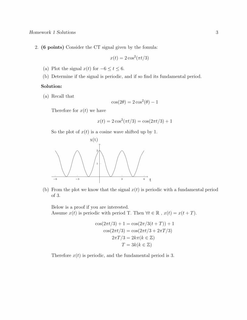
2. (6 points) Consider the CT signal given by the fomula:

x(t) = 2 cos2(πt/3)

(a) Plot the signal x(t) for −6 ≤ t ≤ 6.

(b) Determine if the signal is periodic, and if so find its fundamental period.

Solution:

(a) Recall thatcos(2θ) = 2 cos2(θ)− 1

Therefore for x(t) we have

x(t) = 2 cos2(πt/3) = cos(2πt/3) + 1

So the plot of x(t) is a cosine wave shifted up by 1.

−6 −3 3 6

1

2

t

x(t)

(b) From the plot we know that the signal x(t) is periodic with a fundamental periodof 3.

Below is a proof if you are interested.Assume x(t) is periodic with period T. Then ∀t ∈ R , x(t) = x(t+ T ).

cos(2πt/3) + 1 = cos(2π/3(t+ T )) + 1

cos(2πt/3) = cos(2πt/3 + 2πT/3)

2πT/3 = 2kπ(k ∈ Z)

T = 3k(k ∈ Z)

Therefore x(t) is periodic, and the fundamental period is 3.


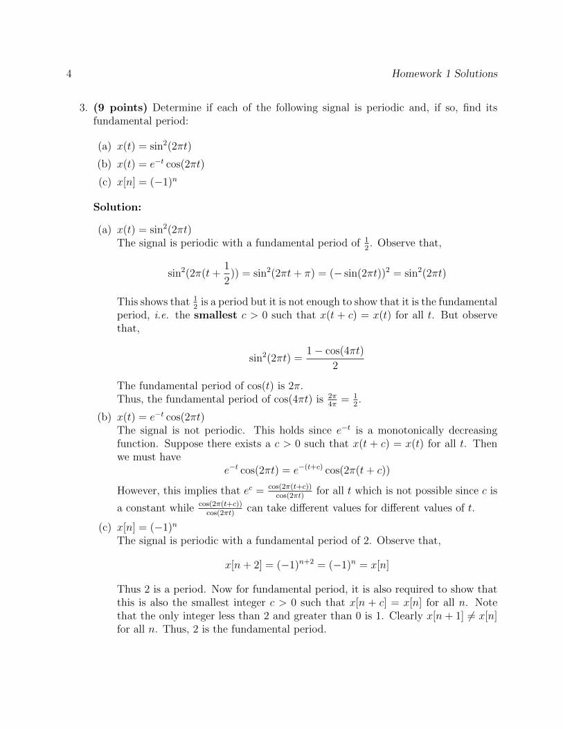
3. (9 points) Determine if each of the following signal is periodic and, if so, find itsfundamental period:

(a) x(t) = sin2(2πt)

(b) x(t) = e−t cos(2πt)

(c) x[n] = (−1)n

Solution:

(a) x(t) = sin2(2πt)The signal is periodic with a fundamental period of 1

2. Observe that,

sin2(2π(t+1

2)) = sin2(2πt+ π) = (− sin(2πt))2 = sin2(2πt)

This shows that 12

is a period but it is not enough to show that it is the fundamentalperiod, i.e. the smallest c > 0 such that x(t + c) = x(t) for all t. But observethat,

sin2(2πt) =1− cos(4πt)

2

The fundamental period of cos(t) is 2π.Thus, the fundamental period of cos(4πt) is 2π

4π= 1

2.

(b) x(t) = e−t cos(2πt)The signal is not periodic. This holds since e−t is a monotonically decreasingfunction. Suppose there exists a c > 0 such that x(t + c) = x(t) for all t. Thenwe must have

e−t cos(2πt) = e−(t+c) cos(2π(t+ c))

However, this implies that ec = cos(2π(t+c))cos(2πt)

for all t which is not possible since c is

a constant while cos(2π(t+c))cos(2πt)

can take different values for different values of t.

(c) x[n] = (−1)n

The signal is periodic with a fundamental period of 2. Observe that,

x[n+ 2] = (−1)n+2 = (−1)n = x[n]

Thus 2 is a period. Now for fundamental period, it is also required to show thatthis is also the smallest integer c > 0 such that x[n + c] = x[n] for all n. Notethat the only integer less than 2 and greater than 0 is 1. Clearly x[n + 1] 6= x[n]for all n. Thus, 2 is the fundamental period.


4. (12 points) Decompose the following signals into their odd and even components.Simplify your answer to the simplest expression:

(a) x(t) = 10t5 + 4t4 − t3 − t2 − 1

(b) x(t) = sin(t) + cos(t)

(c) x(t) = sin(t) cos(t)

(d) x(t) = sin(3t) sin(2t) sin(t) (Hint: sin(−x) = − sin(x))

Solution:

(a) x(t) = 10t5 + 4t4 − t3 − t2 − 1

Odd:1

2(x(t)− x(−t)) = 10t5 − t3

Even:1

2(x(t) + x(−t)) = 4t4 − t2 − 1

Observe that for a general polynomial, the odd powers belong to the odd partand the even powers belong to the even part of the signal.

(b) x(t) = sin(t) + cos(t)

Odd:1

2(x(t)− x(−t)) =

1

2(sin(t) + cos(t)− sin(−t)− cos(−t))

=1

2(sin(t) + cos(t)− (− sin(t))− (cos(t)))

= sin(t)

Even:1

2(x(t) + x(−t)) =

1

2(sin(t) + cos(t) + sin(−t) + cos(−t))

=1

2(sin(t) + cos(t) + (− sin(t)) + (cos(t)))

= cos(t)

Again observe here that sin(t) belongs to the odd part and cos(t) belongs to theeven part of the signal. sin(t) is an odd signal and cos(t) is an even signal.


(c) x(t) = sin(t) cos(t)

Odd:1

2(x(t)− x(−t)) =

1

2(sin(t) cos(t)− sin(−t) cos(−t))

=1

2(sin(t) cos(t)− (− sin(t))(cos(t)))

= sin(t) cos(t)

Even:1

2(x(t) + x(−t)) =

1

2(sin(t) cos(t) + sin(−t) cos(−t))

=1

2(sin(t) cos(t) + (− sin(t))(cos(t)))

= 0

Alternately, observe that sin(t) cos(t) = 12

sin(2t) which is an odd signal.

(d) x(t) = sin(3t) sin(2t) sin(t)

Odd:1

2(x(t)− x(−t)) =

1

2(sin(3t) sin(2t) sin(t)− sin(−3t) sin(−2t) sin(−t))

=1

2(sin(3t) sin(2t) sin(t)− (−1)3 sin(3t) sin(2t) sin(t))

= sin(3t) sin(2t) sin(t)

Even:1

2(x(t) + x(−t)) =

1

2(sin(3t) sin(2t) sin(t) + sin(−3t) sin(−2t) sin(−t))

=1

2(sin(3t) sin(2t) sin(t) + (−1)3 sin(3t) sin(2t) sin(t))

= 0


5. (10 points)

(a) [10 points] Consider the following discrete time signal:

x[n] =

{(12

)n0 ≤ n ≤ 20

0 otherwise

Determine the total energy and average power of x[n].

(b) [10 points] Consider the following continuous time signal:

x(t) =

3t 0 ≤ t ≤ 5

15 5 < t ≤ 10

0 otherwise

Determine the total energy and average power of x(t).

Solution:

(a) Total energy of x[n] is 421−13×420 . To find the total energy,

E =+∞∑

n=−∞

|x[n]|2 =20∑n=0

|x[n]|2 since Signal is 0 elsewhere.

=20∑n=0

(1

2

)2n

=20∑n=0

(1

4

)n=

1− (14)21

1− 14

=421 − 1

3× 420

Average power of x[n] is 0. To find the average power,

P = limN→∞

1

2N + 1

N∑n=−N

|x[n]|2 = limN→∞

1

(2N + 1)

421 − 1

(3× 420)= 0

(b) Total energy of x(t) is 1500. To find the total energy,

E =

∫ +∞

−∞|x(t)|2dt =

∫ 10

0

|x(t)|2dt since Signal is 0 elsewhere.

=

∫ 5

0

(3t)2dt+

∫ 10

5

(15)2dt

= 9

[t3

3

]50

+ (152)[t]105

= 375 + 1125 = 1500


Average power of x(t) is 0. To find the average power,

P = limT→∞

1

2T

∫ +T

−T|x(t)|2dt = lim

T→∞

1

2T1500 = 0

Explanation: Suppose you choose any T > 10, i.e. beyond the range where x(t)is non-zero. Observe that,

E =

∫ +∞

−∞|x(t)|2dt =

∫ −T−∞|x(t)|2dt︸︷︷︸

=0 as signal is 0

+

∫ +T

−T|x(t)|2dt+

∫ ∞+T

|x(t)|2dt︸︷︷︸=0as signal is 0

=

∫ +T

−T|x(t)|2dt for any arbitrary T > 10

Thus,

P = limT→∞

1

2T

∫ +T

−T|x(t)|2dt = lim

T→∞

1

2TE = 0


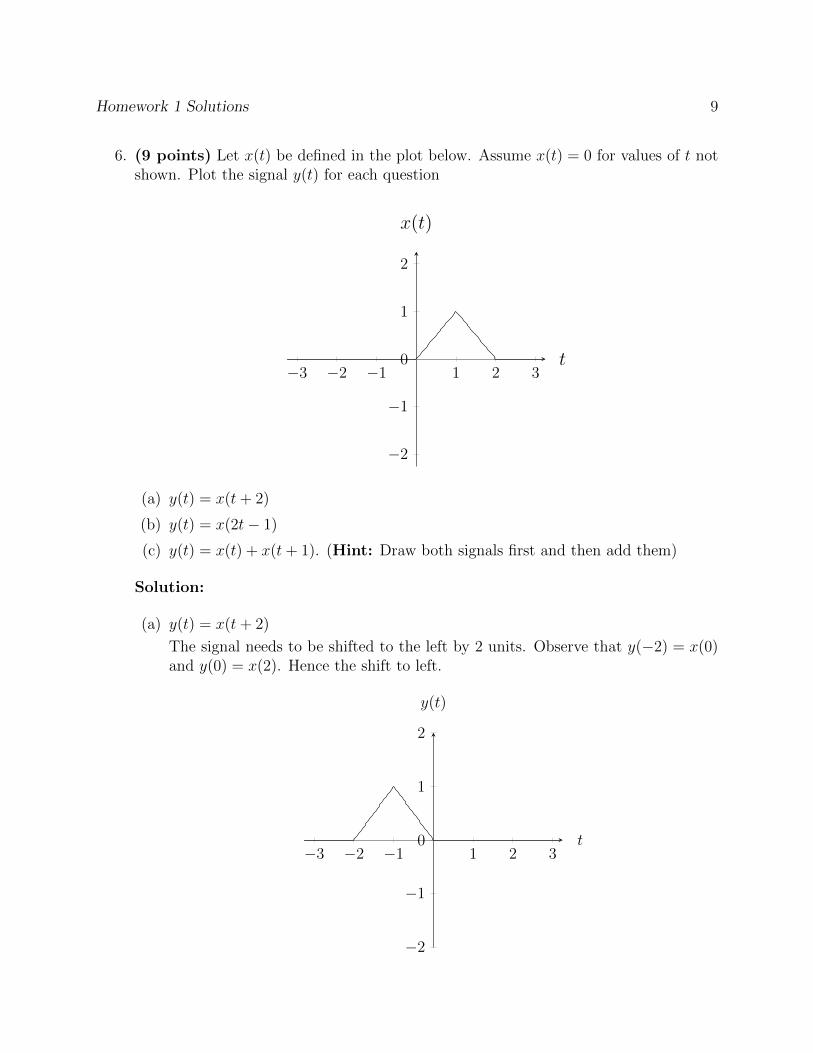
6. (9 points) Let x(t) be defined in the plot below. Assume x(t) = 0 for values of t notshown. Plot the signal y(t) for each question

−3 −2 −1 1 2 3

−2

−1

1

2

0 t

x(t)

(a) y(t) = x(t+ 2)

(b) y(t) = x(2t− 1)

(c) y(t) = x(t) + x(t+ 1). (Hint: Draw both signals first and then add them)

Solution:

(a) y(t) = x(t+ 2)

The signal needs to be shifted to the left by 2 units. Observe that y(−2) = x(0)and y(0) = x(2). Hence the shift to left.

−3 −2 −1 1 2 3

−2

−1

1

2

0 t

y(t)


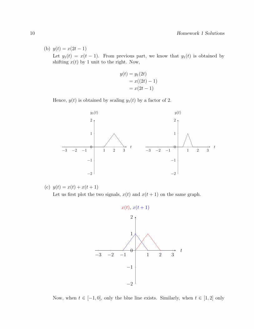
(b) y(t) = x(2t− 1)

Let y1(t) = x(t − 1). From previous part, we know that y1(t) is obtained byshifting x(t) by 1 unit to the right. Now,

y(t) = y1(2t)

= x((2t)− 1)

= x(2t− 1)

Hence, y(t) is obtained by scaling y1(t) by a factor of 2.

−3 −2 −1 1 2 3

−2

−1

1

2

0 t

y1(t)

−3 −2 −1 1 2 3

−2

−1

1

2

0 t

y(t)

(c) y(t) = x(t) + x(t+ 1)

Let us first plot the two signals, x(t) and x(t+ 1) on the same graph.

−3 −2 −1 1 2 3

−2

−1

1

2

0 t

x(t), x(t+ 1)

Now, when t ∈ [−1, 0], only the blue line exists. Similarly, when t ∈ [1, 2] only


the red line exists. When t ∈ [0, 1] there is an overlap. In that domain,

y(t) = (1− x) + (1)

= 1

Hence the complete graph is,

−3 −2 −1 1 2 3

−2

−1

1

2

0 t

y(t)


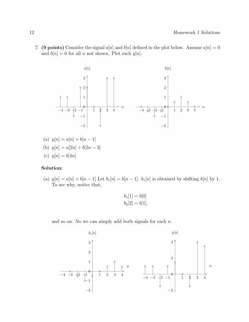
7. (9 points) Consider the signal a[n] and b[n] defined in the plot below. Assume a[n] = 0and b[n] = 0 for all n not shown. Plot each y[n].

−4 −3 −2 −1 1 2 3 4

−2

−1

1

2

3

0 n

a[n]

−4 −3 −2 −1 1 2 3 4

−2

−1

1

2

3

0 n

b[n]

(a) y[n] = a[n] + b[n− 1]

(b) y[n] = a[2n] + b[2n− 3]

(c) y[n] = b[4n]

Solution:

(a) y[n] = a[n] + b[n− 1] Let b1[n] = b[n− 1]. b1[n] is obtained by shifting b[n] by 1.To see why, notice that,

b1[1] = b[0]

b2[2] = b[1],

and so on. No we can simply add both signals for each n.

−4 −3 −2 −1 1 2 3 4

−2

−1

1

2

3

0

n

b1[n]

−4 −3 −2 −1 1 2 3 4

−2

2

4

0

n

y[n]


(b) y[n] = a[2n] + b[2n− 3]

a1[n] = a[2n] can be obtained by skipping every other sample. To get b1[n] =b[2n − 3], we first shift b[n] to the right by 3 units and then skip every othersample

−4 −3 −2 −1 1 2 3 4

−2

−1

1

2

3

0

n

a1[n]

−4 −3 −2 −1 1 2 3 4

−2

−1

1

2

3

0

n

b1[n]

−4 −3 −2 −1 1 2 3 4

−2

2

4

0n

y[n]

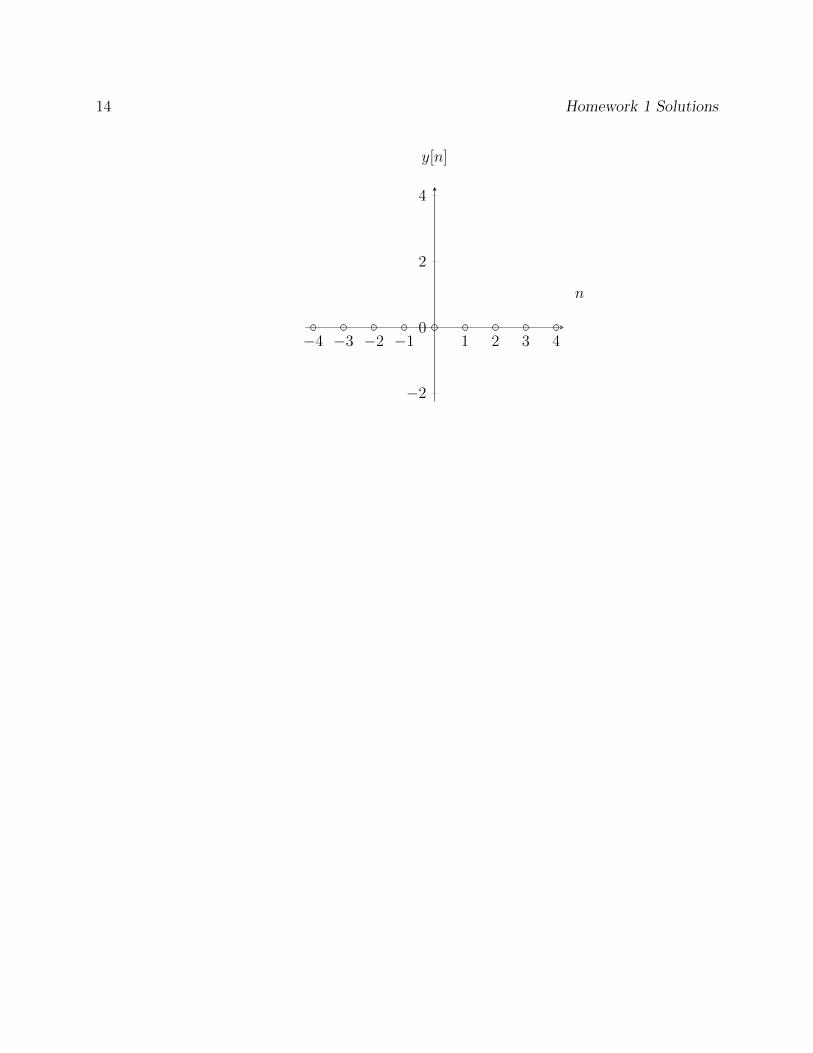
(c) y[n] = b[4n]

Manually evaluating the expression,

y[−2] = b[−8] = 0

y[−1] = b[−4] = 0

y[0] = b[0] = 0

y[1] = b[4] = 0

y[2] = b[8] = 0


−4 −3 −2 −1 1 2 3 4

−2

2

4

0

n

y[n]


Part Two

8. (9 points) MATLAB CommandsPlease download MATLAB using the links here:

http://www.cmu.edu/computing/software/all/matlab/index.html

And the instructions here:

http://www.cmu.edu/computing/software/all/matlab/installation.html

For ECE students, remember to install the standalone edition so that you can useMatlab off campus.When you open MATLAB, there are a few windows to note: a workspace, whichcontains the current variables; and a command window, which allows for the inputof commands. When MATLAB is first opened, both should be empty except for thecommand window prompt.

>>

You can create variables like in other programming languages:

>> a = 2

You will note that the variable a now appears in the workspace. Once you havecreated variables, they will be saved in the workspace and you can use them in yournew commands without having to define them again.Square brackets are used to create matrices. Columns are separated by spaces, and rowsare separated by semicolons. Try the following commands in your MATLAB commandwindow. To get information about any command, you can type help <name of thecommand>.

>> b = [1 2 3]

>> c = [2; 3; 5]

>> d = [1 2 3; 4 5 6]

Try the following MATLAB operators:

>> b*c

>> b+b

>> b+c

>> d*c

Note that if the dimensions do not agree, you cannot use certain operators.

MATLAB has a large library of commands that help to manipulate your matrices. Trythe following commands, and briefly explain what each of the commands do.


Note that MATLAB indexing starts at 1, rather than 0 in many other programminglanguages.

>> a = zeros(4, 3)

>> b = ones(4, 4)

>> c = eye (3)

>> d = size(a)

>> abs([-3, 4])

>> ceil (1.2)

>> help floor

>> e = [2:2:10]

>> f = e’

>> g = e(2)

>> h = cos(pi/2)

>> k = exp (1.0)

>> ex1 = [1.1 2.2 3.3; 4.4 5.5 6.6]

>> n = ex1(1, 2)

>> p = ex1(1,:)

>> m = ex1(1,2:end)

>> q = [p m]

>> cmplx = 3 - 4i

>> real(cmplx)

>> imag(cmplx)

>> abs(cmplx)

>> angle(cmplx)

>> 4^2

>> 3 == 3

>> 3 == 2

>> 3 ~= 1

>> whos

>> clear a b

There are many other built-in functions in MATLAB. MATLAB has excellent docu-mentation, so there are plenty of online resources for helping you find the functionsyou need.Solution:

(1) create 4x3 matrix of zeros

(2) create 4x4 matrix of ones

(3) create 3x3 identity matrix

(4) get the dimensions of matrix a

(5) take the elementwise absolute value of matrix [-3, 4]


(6) round to the higher nearest integer

(7) get help on the selection floor

(8) create a vector e starting with 2 until 10, counting by 2

(9) take the matrix complement of e

(10) take the second element of e

(11) take the cos of (pi/2)

(12) take e to the power of 1

(13) assign matrix

(14) take element of 1st row and second column of ex1

(15) take entire first row of ex1

(16) take first row of ex1 from index 2 to the end

(17) concatenate two vectors

(18) assign complex number 3 - 4i

(19) take the real component of cmplx

(20) take the imaginary component of cmplx

(21) take the absolute value of cmplx

(22) take the angle of cmplx

(23) 4 to the power of 2

(24) test for equality between 3 and 3

(25) test for equality between 3 and 2

(26) test for inequality between 3 and 1

(27) display all variables in workspace

(28) clear the variables a and b


9. (10 points) MATLAB PlotsNow we will get to one of the powerful tools of MATLAB: plots. In order to use theplot function, you need a vector of x coordinates and a vector of y coordinates. Youcan use plot(x, y) to create a continuous line plot.

>> x = [-2:2]

>> y = [1 4 6 7 8];

>> plot(x, y)

You can instead use stem(x, y) to plot discrete points in a stem plot.

>> stem(x, y)

Now, use these tools to make the following graphs, both as a continuous line plot and adiscrete stem plot. Make sure to title your plots and label your axes; try help xlabel,help ylabel, and help title for help on how to do this.

(a) Odd component of y

(b) Even component of y

Solution:

(a) Odd function

>> y = [ 1 4 6 7 8 ] ;>> stem (x , . 5∗ y − . 5∗ y (5 : −1 :1 ) )>> p lo t (x , . 5∗ y − . 5∗ y (5 : −1 :1 ) )

(b) Even function

>> y = [ 1 4 6 7 8 ] ;>> stem (x , . 5∗ y + .5∗ y (5 : −1 :1 ) )>> p lo t (x , . 5∗ y + .5∗ y (5 : −1 :1 ) )


Odd component of y.

Odd component of y.


Even component of y.

Even component of y.


10. (10 points) Matlab FunctionsA square wave, which is also called a pulse wave, is a periodic function that alternatesbetween two values. The duty cycle is the percent of the period in which the signal isat its maximum value. The figure below shows a 1 Hz square wave with equal durationat the maximum value +1 and minimum value 0. So, its duty cycle is 50%.

1 2 3

0.5

1

Time(s)

Am

plitu

de

Now use the functions you examined in question 8 and write your own square wavegenerator. The specifics are:

• The output variable myWave should be a square wave that has a fixed frequencyof 1 Hz and alternates between 1 and 0. The signal lasts for 3 seconds.

• The input variable dutyCycle ranges from 0 to 100 and it controls the durationof the maximum value.

To define a function in Matlab, click on the yellow plus sign on the top left corner ofthe Matlab interface and type in the code below.

function myWave = WaveGenerator(dutyCycle)

# your code here

end

Then save and name the .m file the same name as the function name under your cur-rent working directory. That is, you should save your script as WaveGenerator.m.In your submission, provide the code for this function.

A hint for this problem is to use zeros and ones command. First, let’s look at thefirst 0.5 seconds with a 0.01 second interval. That is, let’s look at the value of thesquare wave plotted above at time points 0.01, 0.02, . . . , 0.5. The amplitude at thesetime points are always 1. So, to get the first half period of a square wave, use

posValue = ones (1 ,50);


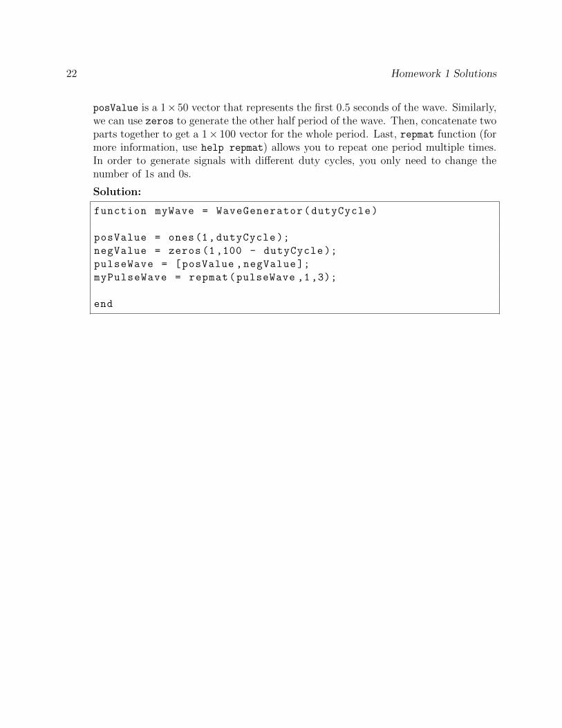
posValue is a 1×50 vector that represents the first 0.5 seconds of the wave. Similarly,we can use zeros to generate the other half period of the wave. Then, concatenate twoparts together to get a 1× 100 vector for the whole period. Last, repmat function (formore information, use help repmat) allows you to repeat one period multiple times.In order to generate signals with different duty cycles, you only need to change thenumber of 1s and 0s.

Solution:

function myWave = WaveGenerator(dutyCycle)

posValue = ones(1, dutyCycle );

negValue = zeros (1,100 - dutyCycle );

pulseWave = [posValue ,negValue ];

myPulseWave = repmat(pulseWave ,1 ,3);

end


11. (9 points) Put it all togetherNow, it is time to use your waveGenerator and the functions you learned from question9 and plot a pulse wave function with 50% duty cycle and 70% duty cycle. To giveyou an example, the code below plots the 20% duty cycle square wave.

t = 0.01:0.01:3;

y = WaveGenerator (20);

plot(t,y)

title (’20% duty cycle square wave ’)

xlabel(’Time/s’)

ylabel(’Amplitude ’)

In your submission, you only need to show the two plots generated.If you can generate plots that look like the figure above, you have already finished yourfirst 18290 homework! Yeah! But if you are a perfectionist, you can try command axis

or adjust LineWidth for plot to make the plot prettier.

Solution:

t = 0.01:0.01:3;

y = WaveGenerator (70);

% change input to 50 for the other question

plot(t,y,’Linewidth ’,3)

set(0, ’DefaultAxesFontSize ’, 15);

title (’70% duty cycle square wave ’)

xlabel(’Time(s)’)

ylabel(’Amplitude ’)

homework 1 solutions - ece.cmu.eduece290/f17/solutions/hw1-solutions.pdf · 18-290 signals and...

Documents