Homework Discussion

• Read pages 446 - 461

• Page 467: 17 – 20, 25 – 27, 61, 62, 63, 67

• See if you can find an example in your life of a survey that might yield unreliable results

The critical issues are:a. Finding a sample that is representative of the population, andb. Determining how big the sample should be.

Choosing a good sample of a reasonable size is more important that the sampling rate.

• Bush's lead gets smaller in poll

• By Susan Page,

• USA TODAY WASHINGTON — President Bush leads Sen. John Kerry by 8 percentage points among likely voters, the latest USA TODAY/ CNN/Gallup Poll shows. That is a smaller advantage than the president held in mid-September but shows him maintaining a durable edge in a race that was essentially tied for months.

Results based on likely voters are based on the sub

sample of 758 survey respondents deemed most

likely to vote in the November 2004 General Election. The margin of

sampling error is ±4 percentage points.

George Gallup explained

• Whether you poll the Unites States or New York State or Baton Rouge … you need… the same number of interviews or samples. It’s no mystery really – if a cook has two pots of soup on the stove, one far larger than the other, and thoroughly stirs them both, he doesn’t have to take more spoonfuls from one than the other to sample the taste accurately.

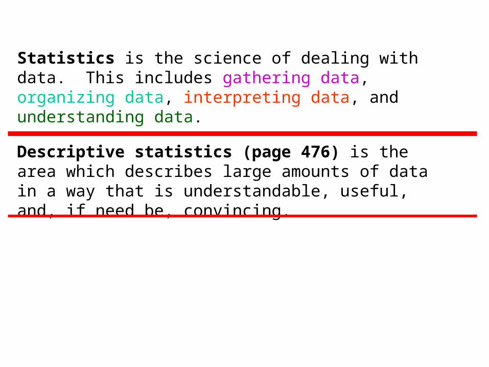
Statistics is the science of dealing with data. This includes gathering data, organizing data, interpreting data, and understanding data.

Descriptive statistics (page 476) is the area which describes large amounts of data in a way that is understandable, useful, and, if need be, convincing.

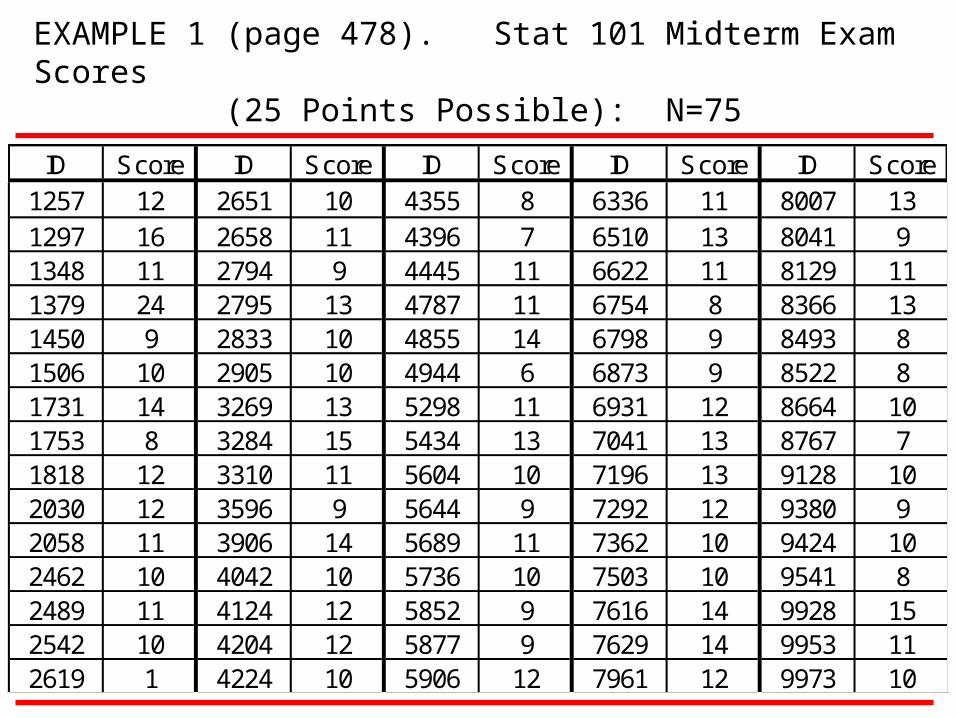
EXAMPLE 1 (page 478). Stat 101 Midterm Exam Scores (25 Points Possible): N=75

ID Score ID Score ID Score ID Score ID Score1257 12 2651 10 4355 8 6336 11 8007 131297 16 2658 11 4396 7 6510 13 8041 91348 11 2794 9 4445 11 6622 11 8129 111379 24 2795 13 4787 11 6754 8 8366 131450 9 2833 10 4855 14 6798 9 8493 81506 10 2905 10 4944 6 6873 9 8522 81731 14 3269 13 5298 11 6931 12 8664 101753 8 3284 15 5434 13 7041 13 8767 71818 12 3310 11 5604 10 7196 13 9128 102030 12 3596 9 5644 9 7292 12 9380 92058 11 3906 14 5689 11 7362 10 9424 102462 10 4042 10 5736 10 7503 10 9541 82489 11 4124 12 5852 9 7616 14 9928 152542 10 4204 12 5877 9 7629 14 9953 112619 1 4224 10 5906 12 7961 12 9973 10

DESCRIPTIVE STATISTICS

A data set is a collection of data values called data points.

The size of a data set is the number of data points in it. We use N to represent size.

EXAMPLE 1 (page 478). Stat 101 Midterm Exam Scores (25 Points Possible): N=75

ID Score ID Score ID Score ID Score ID Score1257 12 2651 10 4355 8 6336 11 8007 131297 16 2658 11 4396 7 6510 13 8041 91348 11 2794 9 4445 11 6622 11 8129 111379 24 2795 13 4787 11 6754 8 8366 131450 9 2833 10 4855 14 6798 9 8493 81506 10 2905 10 4944 6 6873 9 8522 81731 14 3269 13 5298 11 6931 12 8664 101753 8 3284 15 5434 13 7041 13 8767 71818 12 3310 11 5604 10 7196 13 9128 102030 12 3596 9 5644 9 7292 12 9380 92058 11 3906 14 5689 11 7362 10 9424 102462 10 4042 10 5736 10 7503 10 9541 82489 11 4124 12 5852 9 7616 14 9928 152542 10 4204 12 5877 9 7629 14 9953 112619 1 4224 10 5906 12 7961 12 9973 10

When possible values of the numerical variable change by minimum increments, the variable is called discrete

When the differences between the values of a numerical variable can be arbitrarily small, we call the variable continuous

.

Baseball stats

In statistical usage, a variable is any characteristic that varies with members of a population. (page 481)

EXAMPLE 1 (page 478). Stat 101 Midterm Exam Scores (25 Points Possible): N=75

ID Score ID Score ID Score ID Score ID Score1257 12 2651 10 4355 8 6336 11 8007 131297 16 2658 11 4396 7 6510 13 8041 91348 11 2794 9 4445 11 6622 11 8129 111379 24 2795 13 4787 11 6754 8 8366 131450 9 2833 10 4855 14 6798 9 8493 81506 10 2905 10 4944 6 6873 9 8522 81731 14 3269 13 5298 11 6931 12 8664 101753 8 3284 15 5434 13 7041 13 8767 71818 12 3310 11 5604 10 7196 13 9128 102030 12 3596 9 5644 9 7292 12 9380 92058 11 3906 14 5689 11 7362 10 9424 102462 10 4042 10 5736 10 7503 10 9541 82489 11 4124 12 5852 9 7616 14 9928 152542 10 4204 12 5877 9 7629 14 9953 112619 1 4224 10 5906 12 7961 12 9973 10

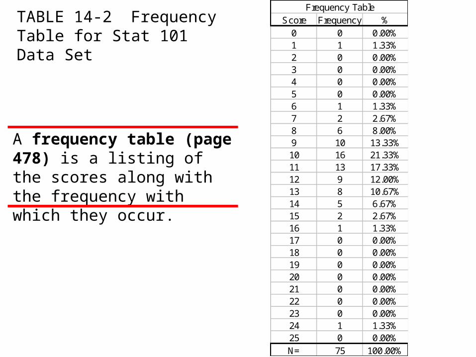
TABLE 14-2 Frequency Table for Stat 101 Data Set

Frequency TableScore Frequency %

0 0 0.00%1 1 1.33%2 0 0.00%3 0 0.00%4 0 0.00%5 0 0.00%6 1 1.33%7 2 2.67%8 6 8.00%9 10 13.33%10 16 21.33%11 13 17.33%12 9 12.00%13 8 10.67%14 5 6.67%15 2 2.67%16 1 1.33%17 0 0.00%18 0 0.00%19 0 0.00%20 0 0.00%21 0 0.00%22 0 0.00%23 0 0.00%24 1 1.33%25 0 0.00%N= 75 100.00%

A frequency table (page 478) is a listing of the scores along with the frequency with which they occur.

02468

1012141618

1 3 5 7 9 11 13 15 17 19 21 23 25

Frequency

Score

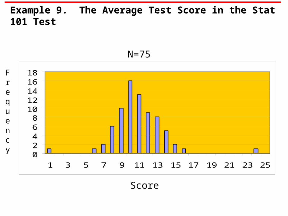
N=75

A bar graph (page 479) is a graph with the possible test scores listed in increasing order on a horizontal axis and the frequency of each test score displayed by the height of the column above that test score.

Outliers are data points that do not fit into the overall pattern of the data.

Objective 7:

Creating structures and systems that model problems and information

Instead of representing frequencies a bar graph may represent relative frequencies i.e. the frequencies expressed as percentages of the total population.

0%2%4%6%8%

10%12%14%16%18%20%22%

1 3 5 7 9

11

13

15

17

19

21

23

25

Rel

ativ

e F

req

uen

cy

N=75

Score

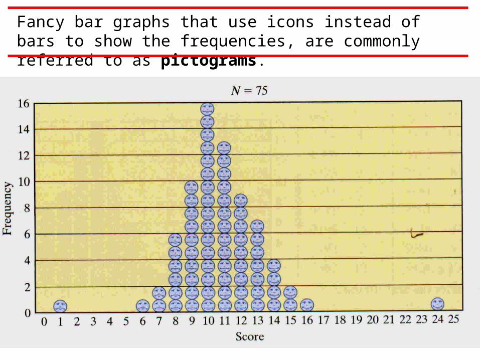
Fancy bar graphs that use icons instead of bars to show the frequencies, are commonly referred to as pictograms.

EXAMPLE 14.3 (page 481).

Yearly sales of XYZ Corporation from 1997 through 2002

Annual Sales (in millions)

50

55

60

65

70

75

80

1997 1998 1999 2000 2001 2002

Year

Mill

ion

s o

f D

olla

rs

Annual Sales (in millions)

01020304050607080

1997 1998 1999 2000 2001 2002

Year

Mill

ion

s o

f D

olla

rs

Year Annual sales1997 521998 551999 612000 632001 702002 77

0

200

400

600

800

1000

1200

40

0-5

00

51

0-6

00

61

0-7

00

71

0-8

00

81

0-9

00

91

0-1

00

0

10

10

-11

00

11

10

-12

00

12

10

-13

00

13

10

-14

00

14

10

-15

00

15

10

-16

00

Fre

qu

en

cy

EXAMPLE (page 484). SAT Scores

400-500 200510-600 300610-700 500710-800 800810-900 1000910-1000 11001010-1100 12001110-1200 9001210-1300 7001310-1400 4001410-1500 3001510-1600 100

When we have a large number of possible scores we often break up the range of scores into class intervals.

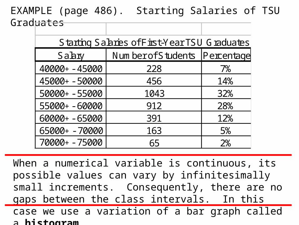
EXAMPLE (page 486). Starting Salaries of TSU Graduates

When a numerical variable is continuous, its possible values can vary by infinitesimally small increments. Consequently, there are no gaps between the class intervals. In this case we use a variation of a bar graph called a histogram.

Starting Salaries of First-Year TSU GraduatesSalary Number of Students Percentage

40000+ - 45000 228 7%45000+ - 50000 456 14%50000+ - 55000 1043 32%55000+ - 60000 912 28%60000+ - 65000 391 12%65000+ - 70000 163 5%70000+ - 75000 65 2%

EXAMPLE (page 486). Starting Salaries of TSU Graduates

When a numerical variable is continuous, its possible values can vary by infinitesimally small increments. Consequently, there are no gaps between the class intervals. In this case we use a variation of a bar graph called a histogram.

N=3258

0%

5%

10%

15%

20%

25%

30%

35%

4000

0-45

000

4500

0-50

000

5000

0-55

000

5500

0-60

000

6000

0-65

000

6500

0-70

000

7000

0-75

000

Per

cen

tag

es

Variables which describe characteristics that cannot be measured numerically are called categorical, or qualitative variables. (page 482)

A variable that represents a measurable quantity is called a numerical or quantitative variable.

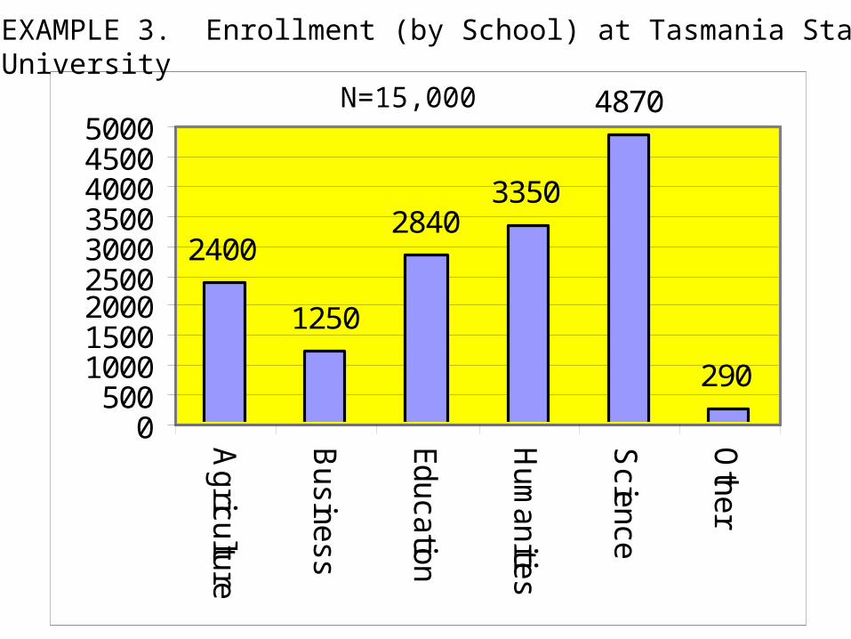
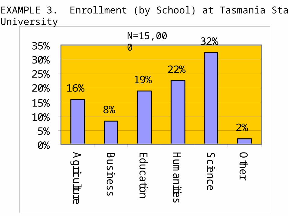
TABLE 14-3 Undergraduate Enrollments at TSUSchool EnrollmentAgriculture 2400 16%Business 1250 8%Education 2840 19%Humanities 3350 22%Science 4870 32%Other 290 2%Total 15000

2400

1250

28403350

4870

290

0500

100015002000250030003500400045005000

Agriculture

Business

Education

Hum

anities

Science

Other

16%

8%

19%22%

32%

2%

0%

5%

10%

15%

20%

25%

30%

35%

Agriculture

Business

Education

Hum

anities

Science

Other

16%

8%

19%

22%

33%

2% Agriculture

Business

Education

Humanities

Science

Other

EXAMPLE 3. Enrollment (by School) at Tasmania State University

2400

1250

28403350

4870

290

0500

100015002000250030003500400045005000

Agric

ultu

re

Busin

ess

Educatio

n

Hum

anitie

s

Scie

nce

Oth

er

N=15,000

EXAMPLE 3. Enrollment (by School) at Tasmania State University

16%

8%

19%22%

32%

2%

0%5%

10%15%

20%25%30%35%

Agric

ultu

re

Busin

ess

Educatio

n

Hum

anitie

s

Scie

nce

Oth

er

N=15,000

EXAMPLE 3. Enrollment (by School) at Tasmania State University

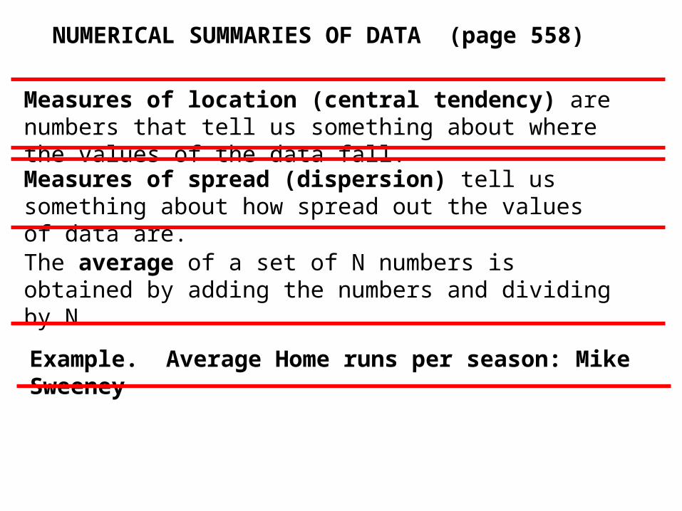
NUMERICAL SUMMARIES OF DATA (page 558)

Measures of location (central tendency) are numbers that tell us something about where the values of the data fall.

The average of a set of N numbers is obtained by adding the numbers and dividing by N.

Example. Average Home runs per season: Mike Sweeney

Measures of spread (dispersion) tell us something about how spread out the values of data are.

TABLE 14-2 Frequency Table for Stat 101 Data Set

Frequency TableScore Frequency %

0 0 0.00%1 1 1.33%2 0 0.00%3 0 0.00%4 0 0.00%5 0 0.00%6 1 1.33%7 2 2.67%8 6 8.00%9 10 13.33%10 16 21.33%11 13 17.33%12 9 12.00%13 8 10.67%14 5 6.67%15 2 2.67%16 1 1.33%17 0 0.00%18 0 0.00%19 0 0.00%20 0 0.00%21 0 0.00%22 0 0.00%23 0 0.00%24 1 1.33%25 0 0.00%N= 75 100.00%

02468

1012141618

1 3 5 7 9 11 13 15 17 19 21 23 25

Frequency

Score

N=75

Example 9. The Average Test Score in the Stat 101 Test

0

1

2

3

4

5

6

7

8

15 16 17 18 19 20 21 22 23

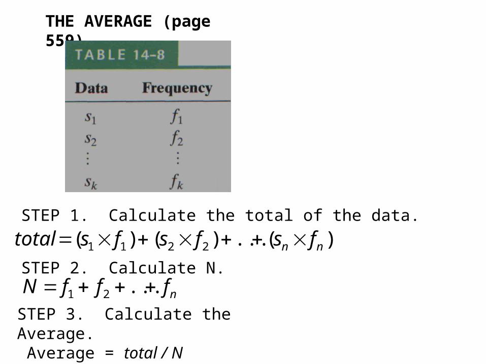
STEP 1. Calculate the total of the data.

)(...)()( 2211 nn fsfsfstotal STEP 2. Calculate N.

nfffN ...21

STEP 3. Calculate the Average. Average = total / N

THE AVERAGE (page 559).

Homework

• Read pages 476 – 489

• Page 499: 1 – 3, 5, 7 – 11, 19, 21, (for 23, 25, 29, 30, 32, find the mean)