homogenization and multiscale...

HomogenizationModeling Flow and Transport

Homogenization and Multiscale Modeling

Ralph E. Showalterhttp://www.math.oregonstate.edu/people/view/show

Department of MathematicsOregon State University

Multiscale Summer School, August, 2008

DOE 98089 “Modeling, Analysis, and Simulation of Multiscale PreferentialFlow’ with Małgorzata Peszynska



IntroductionTwo-scale approximationThe Homogenized problem

Origins

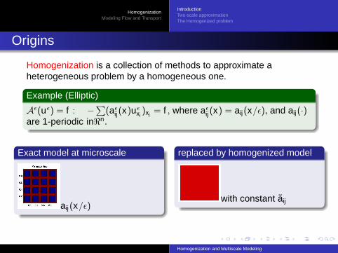
Homogenization is a collection of methods to approximate aheterogeneous problem by a homogeneous one.

Example (Elliptic)

Aε(uε) = f : −∑

(aεij(x)uε

xi)xj = f , where aε

ij(x) = aij(x/ε), and aij(·)are 1-periodic in<n.

Exact model at microscale

aij(x/ε)

replaced by homogenized model

with constant aij




First Issues

Question

Can we find a limiting problem, Au = f , whose solution ucharacterizes the limit, lim

ε→0uε = u ?

Example (Elliptic)

A(u) = f : −∑

(aijuxi )xj = f , where aij are constant.

This is the homogenized equation with effective coefficients.

Question

Is A of the same type as Aε?

The answer is frequently ‘No!’.




An Elliptic Problem

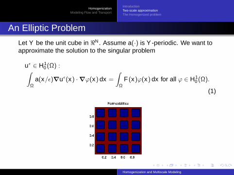
Let Y be the unit cube in <N . Assume a(·) is Y -periodic. We want toapproximate the solution to the singular problem

uε ∈ H10 (Ω) :∫

Ω

a(x/ε)∇uε(x) ·∇ϕ(x) dx =

∫Ω

F (x)ϕ(x) dx for all ϕ ∈ H10 (Ω).

(1)




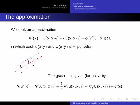
The approximation

We seek an approximation

uε(x) = u(x , x/ε) + εU(x , x/ε) +O(ε2), x ∈ Ω,

in which each u(x , y) and U(x , y) is Y -periodic.

The gradient is given (formally) by

∇uε(x) = ∇xu(x , x/ε) +1ε∇y u(x , x/ε) + ∇y U(x , x/ε) +O(ε).




The solution uε has a bounded gradient, so ∇y u(x , y) = 0 and

uε(x) = u(x) + εU(x , x/ε) +O(ε2) (2a)

∇uε(x) = ∇u(x) + ∇y U(x , x/ε) +O(ε) (2b)

Substitute (2) into (1) with a test function of the same form

ϕ(x) + εΦ(x , x/ε)

where Φ(x , y) is Y -periodic for each x ∈ Ω.




The variational form

Two-scale limits ε → 0 give the system

u ∈ H10 (Ω), U ∈ L2(Ω, H1

#(Y )) :∫Ω

∫Y

a(y)(∇u(x) + ∇y U(x , y)) · (∇ϕ(x) + ∇yΦ(x , y)) dy dx

=

∫Ω

F (x)ϕ(x) dx for all ϕ ∈ H10 (Ω), Φ ∈ L2(Ω, H1

#(Y )). (3)




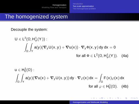
The homogenized system

Decouple the system:

U ∈ L2(Ω, H1#(Y )) :∫

Ω

∫Y

a(y)(∇y U(x , y) + ∇u(x)) ·∇yΦ(x , y) dy dx = 0

for all Φ ∈ L2(Ω, H1#(Y )). (4a)

u ∈ H10 (Ω) :∫

Ω

∫Y

a(y)(∇u(x) + ∇y U(x , y)) dy ·∇ϕ(x) dx =

∫Ω

F (x)ϕ(x) dx

for all ϕ ∈ H10 (Ω). (4b)




The Cell problem

The local problem (4a) is equivalent to requiring

U(x , ·) ∈ H1#(Y ) :∫

Ya(y)(∇y U(x , y) + ∇u(x)) ·∇yΦ(y) dy = 0 for all Φ ∈ H1

#(Y ).

Define ωi(y) for each 1 ≤ i ≤ N to be the solution of the cell problem

ωi ∈ H1#(Y ) :

∫Y

a(y)(∇yωi(y)+ei)·∇yΦ(y) dy = 0 for all Φ ∈ H1#(Y ).

(5)where ei is the indicated coordinate vector in <N .




The Homogenized problem

By linearity the solution is given by

U(x , y) =i=N∑i=1

∂iu(x)ωi(y)

This is substituted into (4b) to obtain

u ∈ H10 (Ω) : ∫

Ω

aij∂iu(x) · ∂jϕ(x) dx =

∫Ω

F (x)ϕ(x) dx

for all ϕ ∈ H10 (Ω). (6)

where the constant coefficients are given by

aij =

∫Y

a(y)(δij + ∂jωi(y)

)dy . (7)




The approximate solution

uε(x) = u(x) + ε ∇u(x) · (ω1(x/ε), ω2(x/ε), . . . , ωN(x/ε)) +O(ε2) ,

∇uε(x) =

∇u(x) + ∇u(x) · (∇ω1(x/ε), ∇ω2(x/ε), . . . , ∇ωN(x/ε)) +O(ε)

of the singular elliptic problem.




Homogenization

Alain Bensoussan, Jacques-Louis Lions, and George Papanicolaou.Asymptotic analysis for periodic structures, volume 5 of Studies inMathematics and its Applications.North-Holland Publishing Co., Amsterdam, 1978.

Enrique Sanchez-Palencia.Nonhomogeneous media and vibration theory, volume 127 of LectureNotes in Physics.Springer-Verlag, Berlin, 1980.

V. V. Jikov, S. M. Kozlov, and O. A. Oleinik.Homogenization of differential operators and integral functionals.Springer-Verlag, Berlin, 1994.



Multiscale Flow and TransportThe Classical CaseThe Highly-Heterogeneous CaseThe Affine CouplingComputational Experiments

Multiscale Flow and Transport ... the model

u(x) = −K(x)∇p(x), ∇ · u(x) = 0

φ∂c(x , t)

∂t+∇ · (u(x)c(x , t)− D(u(x))∇c(x , t)) = 0

Kfast , Kslow → ufast , uslow → Dfast , Dslow




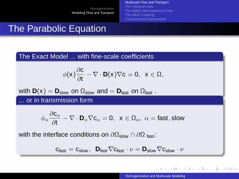
The Parabolic Equation

The Exact Model ... with fine-scale coefficients

φ(x)∂c∂t

−∇ · D(x)∇c = 0, x ∈ Ω,

with D(x) = Dslow on Ωslow and = Dfast on Ωfast .... or in transmission form

φα∂cα

∂t−∇ · Dα∇cα = 0, x ∈ Ωα, α = fast , slow

with the interface conditions on ∂Ωslow ∩ ∂Ω fast :

cfast = cslow , Dfast∇cfast · ν = Dslow∇cslow · ν




The Classical Case

The coefficients are D = [Dfast , Dslow ] :

φ∂c∂t

−∇ · D∇c = 0

The fine-scale geometry is eliminated . . .. . . replaced by the constant effective coefficient D.

The upscaled limit is of the same type . . . a single equation.

The fast and slow regions are coupled by gradients of thesolution (flux) .

Accurate only in this low contrast case.




... the algorithmExact model at microscale

D(x) = Dslow , Dfast

replaced by homogenized model

with constant D

Compute homogenized coefficient D = D(Dfast , Dslow )

Djk =1|Ω0|

∫Ω0

Djk (y)(δjk + ∂kωj(y))dA

−∇ · D(y)∇ωj(y) = ∇ · (D(y)ej),ωj(y) is Ω0 − periodic.

It works well for problems with low contrast Dfast/Dslow




The Obstacle Problem . . . a special case

The coefficients are D = [Dfast , 0] :

φ0 ∂c0

∂t−∇ · D0∇c0 = 0

The slow region Ωslow is impervious.




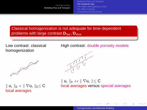
Classical homogenization is not adequate for time-dependentproblems with large contrast Dfast/Dslow

Low contrast: classicalhomogenization

‖ uε ‖0 + ‖ ∇uε ‖0≤ Clocal averages

High contrast: double porosity models

‖ uε ‖0 +ε ‖ ∇uε ‖≤ Clocal averages versus special averages




The Double-porosity model

The coefficients are D = [Dfast , ε20Dslow ] :

φ0 ∂c∂t

+∑

i

χiqi(t)−∇ · D0∇c = 0, qi(t) =1

|Ωi |

∫Γi

Dslow∇ci · νds,

φslow∂ci

∂t−∇ · Dslow∇ci = 0, ci |Γi =

1

|Ωi |

∫Ωi

c(x)dA.

The upscaled model is a system, highly parallel.

The coupling from the cell to global equation is via gradients.

The coupling from the global equation to the cell is via the values.

The contribution of the cells is a secondary storage.

Accurate only in this high contrast case.

It will not couple any advective effects to the local cell.




Double-porosity Micro-structure ModelExact model replaced by two

layers

+

Global equation, x ∈ Ω

φ0 ∂c∂t

+∑

i

χiqi(t)−∇ · D0∇c = 0

qi(t) = Π∗0,i(Dslow∇ci(·, t) · ν)

Cell problem at each x ∈ Ωi

φslow∂ci

∂t− ∇ · Dslow∇ci = 0

ci |Γi = Π0,i(c)(t)




Notes

The coefficients in the global equation are precisely those of theobstacle problem.

The cell input to the global equation is

qi(t) =1

|Ωi |∂

∂t

∫Ωi

φslow ci(x, t) dx

. . . the rate of secondary storage.

The spatially-constant input to the cell problem will not transmitany advective transport.

We shall more tightly couple the cell by replacing the constantcoupling with an affine coupling to the surrounding fast medium. Thiswill provide a gradient coupling.




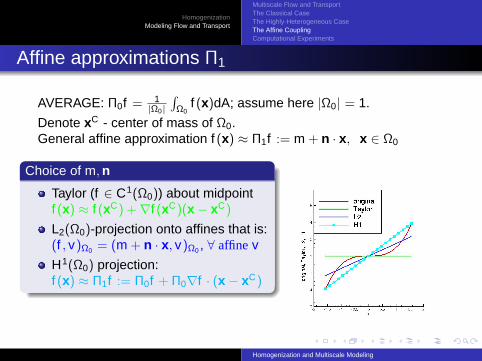
Affine approximations Π1

AVERAGE: Π0f = 1|Ω0|

∫Ω0

f (x)dA; assume here |Ω0| = 1.

Denote xC - center of mass of Ω0.General affine approximation f (x) ≈ Π1f := m + n · x, x ∈ Ω0

Choice of m, n

Taylor (f ∈ C1(Ω0)) about midpointf (x) ≈ f (xC) +∇f (xC)(x − xC)

L2(Ω0)-projection onto affines that is:(f , v)Ω0 = (m + n · x, v)Ω0 , ∀ affinev

H1(Ω0) projection:f (x) ≈ Π1f := Π0f + Π0∇f · (x − xC)




Summary: the affine coupling Πi and its dual Π∗i

Affine coupling Πi : H1(Ω) 7→ H1(Ωi)

Πi(w)(x) ≡ Π0w + Π0(∇w) · (x − xC)

Its dual Π∗i : H1(Ωi)

∗ 7→ H1(Ω)∗ pointwise

Π∗i (q)(x) = χi(x)M0

i (q)−∇ · χi(x)M1i (q)




Double-porosity Model with secondary flux

φ0 ∂c∂t

+∑

i

χiqi(t)−∇ · D0∇c = 0,

φslow∂ci

∂t−∇ · Dslow∇ci = 0,

ci |Γi =1

|Ωi |

∫Ωi

cdA +1

|Ωi |

∫Ωi

∇c dA · (x − xC).

qi(t) =1

|Ωi |

∫Γi

Dslow∇ci · νds −∇ · χi(x)

|Ωi |

∫Γi

Dslow∇ci · ν (x − xC)dS

This is∂

∂t(secondary storage) −∇· (secondary flux) from the local

cells.




Computational experiments at microscaleGOAL: reproduce qualitatively experimental results




Porous Media

Ulrich Hornung, editor.Homogenization and Porous Media, volume 6 of InterdisciplinaryApplied Mathematics.Springer-Verlag, New York, 1997.

Peszynska, M.; Showalter, R. E.Multiscale Elliptic-Parabolic Systems for Flow and Transport ,Electron. J. Differential Equations 2007, No. 147, 30 pp. (electronic).http://ejde.math.txstate.edu/Volumes/2007/147/abstr.html

Brendan Zinn, Lucy C. Meigs, Charles F. Harvey, Roy Haggerty,Williams J. Peplinski, and Claudius Freiherr von Schwerin.Experimental visualization of solute transport and mass transferprocesses in two-dimensional conductivity fields with connectedregions of high conductivity.Environ Sci. Technol., 38:3916–3926, 2004.


homogenization and multiscale...

Documents