homogenization and other multi-scale problems in...
TRANSCRIPT

Homogenization and other multi-scale problemsin Bellman-Isaacs equations
Martino Bardi
Dipartimento di Matemetica Pura ed ApplicataUniversità di Padova
New Trends in Analysis and Control of Nonlinear PDEsRoma, June 13–15, 2011
Martino Bardi (Università di Padova) Multi-scale Bellman-Isaacs Roma, June 15th, 2011 1 / 29

Plan
1 Homogenization of non-coercive Hamilton–Jacobi equations(joint work with G. Terrone)
I Some previous results
I Examples of non-homogenization
I Homogenization on subspaces
I Convex-concave eikonal equations and differential games
2 Optimal control with stochastic volatility(joint work with A. Cesaroni and L. Manca)
I Motivation: financial models
I Singular perturbations of H-J-B equations
I Merton portfolio optimization with stochastic volatility
Martino Bardi (Università di Padova) Multi-scale Bellman-Isaacs Roma, June 15th, 2011 2 / 29
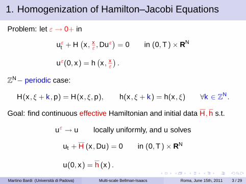
1. Homogenization of Hamilton–Jacobi Equations
Problem: let ε → 0+ in
uεt + H
(x , x
ε , Duε)
= 0 in (0, T )× RN
uε(0, x) = h(x , x
ε
).
ZN− periodic case:
H(x , ξ + k , p) = H(x , ξ, p), h(x , ξ + k) = h(x , ξ) ∀k ∈ ZN .
Goal: find continuous effective Hamiltonian and initial data H, h s.t.
uε → u locally uniformly, and u solves
ut + H (x , Du) = 0 in (0, T )× RN
u(0, x) = h (x) .
Martino Bardi (Università di Padova) Multi-scale Bellman-Isaacs Roma, June 15th, 2011 3 / 29
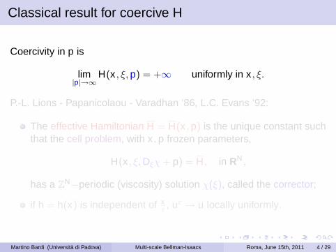
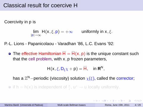
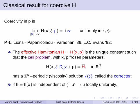
Classical result for coercive H
Coercivity in p is
lim|p|→∞
H(x , ξ, p) = +∞ uniformly in x , ξ.
P.-L. Lions - Papanicolaou - Varadhan ’86, L.C. Evans ’92:
The effective Hamiltonian H = H(x , p) is the unique constant suchthat the cell problem, with x , p frozen parameters,
H(x , ξ, Dξχ + p) = H, in RN ,
has a ZN−periodic (viscosity) solution χ(ξ), called the corrector;
if h = h(x) is independent of xε , uε → u locally uniformly.
Martino Bardi (Università di Padova) Multi-scale Bellman-Isaacs Roma, June 15th, 2011 4 / 29

The effective initial data
If the initial data h = h(x , xε ) must find the initial condition h(x).
O. Alvarez - M. B. (ARMA ’03):Assume there exists the recession function of H
H ′(x , ξ, p) := limλ→+∞
H(x , ξ, λp)
λ.
Consider, for frozen x , wt + H ′(x , ξ, Dξw) = 0, w(0, ξ) = h(x , ξ).
If limt→+∞ w(t , ξ) = constant =: h(x),
then limt→0 limε→0 uε = h(x).
In the coercive case h (x) = minξh(x , ξ).
Martino Bardi (Università di Padova) Multi-scale Bellman-Isaacs Roma, June 15th, 2011 5 / 29
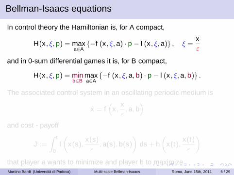
Bellman-Isaacs equations
In control theory the Hamiltonian is, for A compact,
H(x , ξ, p) = maxa∈A
{−f (x , ξ, a) · p − l (x , ξ, a)} , ξ =xε
and in 0-sum differential games it is, for B compact,
H(x , ξ, p) = minb∈B
maxa∈A
{−f (x , ξ, a, b) · p − l (x , ξ, a, b)} .
The associated control system in an oscillating periodic medium is
x = f(
x ,xε, a, b
)and cost - payoff
J :=
∫ t
0l(
x(s),x(s)
ε, a(s), b(s)
)ds + h
(x(t),
x(t)ε
)that player a wants to minimize and player b to maximize.Martino Bardi (Università di Padova) Multi-scale Bellman-Isaacs Roma, June 15th, 2011 6 / 29
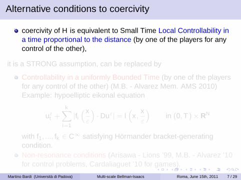
Alternative conditions to coercivity
coercivity of H is equivalent to Small Time Local Controllability ina time proportional to the distance (by one of the players for anycontrol of the other),
it is a STRONG assumption, can be replaced by
Controllability in a uniformly Bounded Time (by one of the playersfor any control of the other) (M.B. - Alvarez Mem. AMS 2010)Example: hypoelliptic eikonal equation
uεt +
k∑i=1
|fi(x
ε
)· Duε| = l
(x ,
xε
)in (0, T )× RN
with f1, ..., fk ∈ C∞ satisfying Hörmander bracket-generatingcondition.Non-resonance conditions (Arisawa - Lions ’99, M.B. - Alvarez ’10for control problems, Cardaliaguet ’10 for games).
Martino Bardi (Università di Padova) Multi-scale Bellman-Isaacs Roma, June 15th, 2011 7 / 29
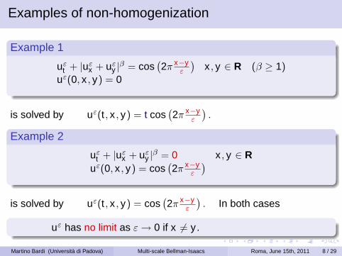
Examples of non-homogenization
Example 1
uεt + |uε
x + uεy |β = cos
(2π x−y
ε
)x , y ∈ R (β ≥ 1)
uε(0, x , y) = 0
is solved by uε(t , x , y) = t cos(2π x−y
ε
).
Example 2
uεt + |uε
x + uεy |β = 0 x , y ∈ R
uε(0, x , y) = cos(2π x−y
ε
)is solved by uε(t , x , y) = cos
(2π x−y
ε
). In both cases
uε has no limit as ε → 0 if x 6= y .
Martino Bardi (Università di Padova) Multi-scale Bellman-Isaacs Roma, June 15th, 2011 8 / 29

Example 3
uεt + |uε
x | − |uεy | = cos
(2π x−y
ε
)x , y ∈ R
uε(0, x , y) = 0
is solved by uε(t , x , y) = t cos(2π x−y
ε
).
Example 4
uεt + |uε
x | − |uεy | = 0 x , y ∈ R
uε(0, x , y) =(2π x−y
ε
)is solved by uε(t , x , y) = cos
(2π x−y
ε
).
Again
uε has no limit as ε → 0 if x 6= y .
Martino Bardi (Università di Padova) Multi-scale Bellman-Isaacs Roma, June 15th, 2011 9 / 29
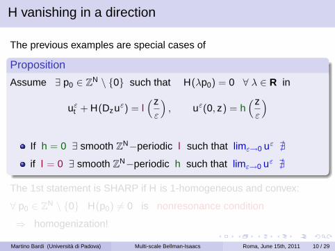
H vanishing in a direction
The previous examples are special cases of
Proposition
Assume ∃ p0 ∈ ZN \ {0} such that H(λp0) = 0 ∀ λ ∈ R in
uεt + H(Dzuε) = l
(zε
), uε(0, z) = h
(zε
)
If h = 0 ∃ smooth ZN−periodic l such that limε→0 uε @
if l = 0 ∃ smooth ZN−periodic h such that limε→0 uε @
The 1st statement is SHARP if H is 1-homogeneous and convex:
∀ p0 ∈ ZN \ {0} H(p0) 6= 0 is nonresonance condition
⇒ homogenization!
Martino Bardi (Università di Padova) Multi-scale Bellman-Isaacs Roma, June 15th, 2011 10 / 29

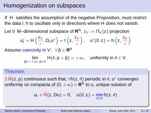
Homogenization on subspaces
If H satisfies the assumption of the negative Proposition, must restrictthe data l , h to oscillate only in directions where H does not vanish.
Let V M–dimensional subspace of RN , zV := ΠV (z) projection
uεt + H
(zV
ε, Dzuε
)= l(
z,zV
ε
), uε(0, z) = h
(z,
zV
ε
)Assume coercivity in V : ∀ p ∈ RN
lim|p|→+∞, p∈V
H(θ, p + p) = +∞, uniformly in θ ∈ V .
Theorem
∃ H(z, p) continuous such that, ∀h(z, θ) periodic in θ, uε convergesuniformly on compacta of (0,+∞)× RN to u, unique solution of
ut + H(z, Du) = 0, u(0, z) = minθ∈V
h(z, θ)
Martino Bardi (Università di Padova) Multi-scale Bellman-Isaacs Roma, June 15th, 2011 11 / 29
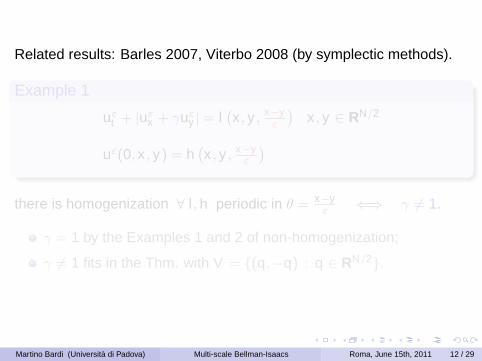
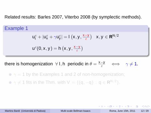
Related results: Barles 2007, Viterbo 2008 (by symplectic methods).
Example 1
uεt + |uε
x + γuεy | = l
(x , y , x−y
ε
)x , y ∈ RN/2
uε(0, x , y) = h(x , y , x−y
ε
)there is homogenization ∀ l , h periodic in θ = x−y
ε ⇐⇒ γ 6= 1.
γ = 1 by the Examples 1 and 2 of non-homogenization;
γ 6= 1 fits in the Thm. with V = {(q,−q) : q ∈ RN/2}.
Martino Bardi (Università di Padova) Multi-scale Bellman-Isaacs Roma, June 15th, 2011 12 / 29
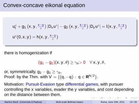
Convex-concave eikonal equation
uεt + g1
(x , y , x−y
ε
)|Dxuε| − g2
(x , y , x−y
ε
)|Dyuε| = l(x , y , x−y
ε )
uε(0, x , y) = h(x , y , x−yε )
there is homogenization if
(g1 − g2)(x , y , θ) ≥ γo> 0 ∀ x , y , θ,
or, symmetrically, g2 − g1 ≥ γo.Proof: by the Thm. with V = {(q,−q) : q ∈ RN/2}.
Motivation: Pursuit-Evasion type differential games, with pursuercontrolling the x variables, evader the y variables, and cost dependingon the distance between them.
Martino Bardi (Università di Padova) Multi-scale Bellman-Isaacs Roma, June 15th, 2011 13 / 29
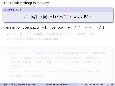
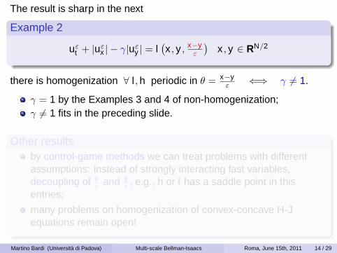
The result is sharp in the next
Example 2
uεt + |uε
x | − γ|uεy | = l
(x , y , x−y
ε
)x , y ∈ RN/2
there is homogenization ∀ l , h periodic in θ = x−yε ⇐⇒ γ 6= 1.
γ = 1 by the Examples 3 and 4 of non-homogenization;γ 6= 1 fits in the preceding slide.
Other resultsby control-game methods we can treat problems with differentassumptions: instead of strongly interacting fast variables,decoupling of x
ε and yε , e.g., h or l has a saddle point in this
entries;
many problems on homogenization of convex-concave H-Jequations remain open!
Martino Bardi (Università di Padova) Multi-scale Bellman-Isaacs Roma, June 15th, 2011 14 / 29

2. Optimal control with stochastic volatility
In Financial Mathematics the evolution of a stock S is described by
d log Ss = γ ds + σ dWs
and the classical Black-Scholes formula for the option pricing problemis derived assuming the parameters are constants.
However the volatility σ is not really a constant, it rather looks like anergodic mean-reverting stochastic process, so it is often modeled asσ(ys) with ys an Ornstein-Uhlenbeck diffusion process.It is argued in the book
Fouque, Papanicolaou, Sircar: Derivatives in financial markets withstochastic volatility, 2000,
that the process ys also evolves on a faster time scale than the stockprices. Next picture shows the typical bursty behavior.
Martino Bardi (Università di Padova) Multi-scale Bellman-Isaacs Roma, June 15th, 2011 15 / 29

Martino Bardi (Università di Padova) Multi-scale Bellman-Isaacs Roma, June 15th, 2011 16 / 29

The model with fast stochastic volatility σ proposed in [FPS] is
d log Ss = γ ds + σ(ys) dWs
dys = 1ε (m − ys) + ν√
εdWs
For the option pricing problem the limit is given by the Black-Scholesformula of the model with (constant) mean historical volatility
d log Ss = γ ds + σ dWs, σ2 =
∫R
σ2(y)e−(y−m)2/2ν2
√2πν2
dy ,
the mean being w.r.t. the (Gaussian) invariant measure of theOrnstein-Uhlenbeck process driving ys.
Martino Bardi (Università di Padova) Multi-scale Bellman-Isaacs Roma, June 15th, 2011 17 / 29
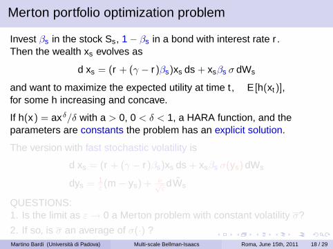
Merton portfolio optimization problem
Invest βs in the stock Ss, 1− βs in a bond with interest rate r .Then the wealth xs evolves as
d xs = (r + (γ − r)βs)xs ds + xsβs σ dWs
and want to maximize the expected utility at time t , E [h(xt)],for some h increasing and concave.
If h(x) = axδ/δ with a > 0, 0 < δ < 1, a HARA function, and theparameters are constants the problem has an explicit solution.
The version with fast stochastic volatility is
d xs = (r + (γ − r)βs)xs ds + xsβs σ(ys) dWs
dys = 1ε (m − ys) + ν√
εdWs
QUESTIONS:1. Is the limit as ε → 0 a Merton problem with constant volatility σ?
2. If so, is σ an average of σ(·) ?Martino Bardi (Università di Padova) Multi-scale Bellman-Isaacs Roma, June 15th, 2011 18 / 29

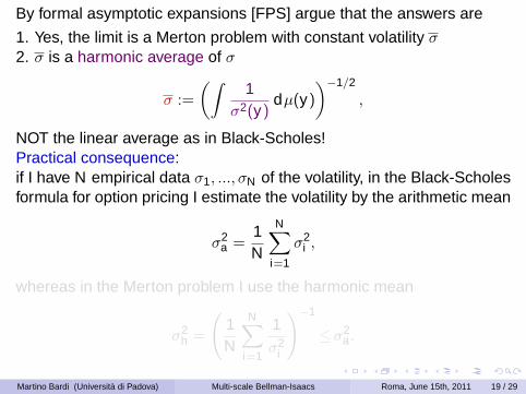
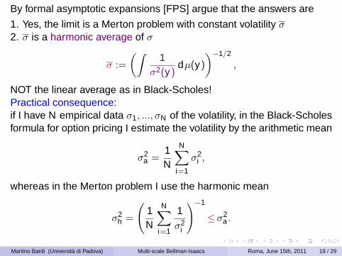
By formal asymptotic expansions [FPS] argue that the answers are
1. Yes, the limit is a Merton problem with constant volatility σ2. σ is a harmonic average of σ
σ :=
(∫1
σ2(y)dµ(y)
)−1/2
,
NOT the linear average as in Black-Scholes!Practical consequence:if I have N empirical data σ1, ..., σN of the volatility, in the Black-Scholesformula for option pricing I estimate the volatility by the arithmetic mean
σ2a =
1N
N∑i=1
σ2i ,
whereas in the Merton problem I use the harmonic mean
σ2h =
(1N
N∑i=1
1σ2
i
)−1
≤σ2a.
Martino Bardi (Università di Padova) Multi-scale Bellman-Isaacs Roma, June 15th, 2011 19 / 29

Conclusion: the correct average seems to depend on the problem!
QUESTIONS:
Why?
Can the formula for the Merton problem be rigorously justified andwhat is the convergence as ε → 0?
Is there a unified "formula" for the two problems and for othersimilar problems?
Note: the Black-Scholes model has no control, the associated PDE isa heat-type linear equation;
Merton is a stochastic control problem whose Hamilton-Jacobi-Bellmanequation is fully nonlinear and degenerate parabolic.
I’ll present a result on two-scale Hamilton-Jacobi-Bellman equationsthat will answer these (and other) questions.
Martino Bardi (Università di Padova) Multi-scale Bellman-Isaacs Roma, June 15th, 2011 20 / 29

The H-J approach to Singular Perturbations
Control system
dxs = f (xs, ys, αs) ds + σ(xs, ys, αs) dWs, xs ∈ Rn, αs ∈ A,
dys = 1ε g(xs, ys) ds + 1√
εν(xs, ys) dWs, ys ∈ Rm,
x0 = x , y0 = y
Cost functional Jε(t , x , y , α) :=∫ t
0 l(xs, ys, αs) ds + h(xt , yt)
Value function
uε(t , x , y) := infα∈A(t)
E [Jε(t , x , y , α)]
A(t) admisible controls on [0, t ].
GOAL: let ε → 0 and find a simplified model.
Martino Bardi (Università di Padova) Multi-scale Bellman-Isaacs Roma, June 15th, 2011 21 / 29

Assumptions on data:
h continuous, supy h(x , y) ≤ K (1 + |x |2)
f , σ, g, τ, l Lipschitz in (x , y) (unif. in α) with linear growth
Then uε solves the HJB equation
∂uε
∂t+H
(x , y , Dxuε, D2
xxuε,1√ε
D2xyuε
)− 1
εLuε = 0 in R+×Rn ×Rm,
H (x , y , p, M, Z ) := maxa∈A
{−tr(σσT M)− f · p − l − tr(σνZ T )
}L := tr(ννT D2
yy ) + g · Dy .
Theorem (Da Lio - Ley). The value function uε is the unique viscositysolution with growth uε(t , x , y) ≤ C(1 + |x |2 + |y |2) of the Cauchyproblem with initial condition
uε(0, x , y) = h(x , y).
Martino Bardi (Università di Padova) Multi-scale Bellman-Isaacs Roma, June 15th, 2011 22 / 29

Next assume on the linear operator L
Ellipticity: ∃Λ(y) > 0 s.t. ∀ x ν(x , y)νT (x , y) ≥ Λ(y)I
Lyapunov: ∃w ∈ C(Rm), k > 0, R0 > 0 s.t.−Lw ≥ k for |y | > R0, ∀x ,
w(y) → +∞ as |y | → +∞.
Then,
the fast subsystem rescaled by τ = s/ε and with x ∈ Rn frozen
(FS) dyτ = g(x , yτ ) dτ + ν(x , yτ ) dWτ ,
is uniquely ergodic, i.e., has a unique invariant measure µx .
Liouville property:any bounded subsolution of −Lv = 0 is constant.
Martino Bardi (Università di Padova) Multi-scale Bellman-Isaacs Roma, June 15th, 2011 23 / 29
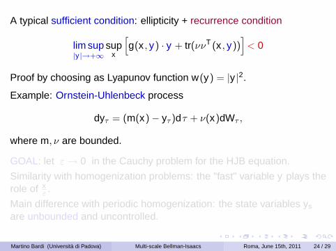
A typical sufficient condition: ellipticity + recurrence condition
lim sup|y |→+∞
supx
[g(x , y) · y + tr(ννT (x , y))
]< 0
Proof by choosing as Lyapunov function w(y) = |y |2.
Example: Ornstein-Uhlenbeck process
dyτ = (m(x)− yτ )dτ + ν(x)dWτ ,
where m, ν are bounded.
GOAL: let ε → 0 in the Cauchy problem for the HJB equation.
Similarity with homogenization problems: the "fast" variable y plays therole of x
ε .
Main difference with periodic homogenization: the state variables ys
are unbounded and uncontrolled.
Martino Bardi (Università di Padova) Multi-scale Bellman-Isaacs Roma, June 15th, 2011 24 / 29

Convergence Theorem
Under the previous assumptions, the (weak) limit u(t , x) as ε → 0 ofthe value function uε(t , x , y) solves
(CP)
∂u∂t +
∫H(x , y , Dxu, D2
xxu, 0)
dµx(y) = 0 in R+ × Rn
u(0, x) =∫
h(x , y) dµx(y)
If, moreover, either g, ν do not depend on x or
g(x , ·), ν(x , ·) ∈ C1 and g(·, y), ν(·, y) ∈ C1b
Dxg, Dyg, Dxν, Dyν are Hölder in y uniformly w.r.t. x ,
then u is the unique viscosity solution (with quadratic growth) of (CP)
and uε(t , x , y) → u(t , x) locally uniformly on (0,+∞)× Rn.
Martino Bardi (Università di Padova) Multi-scale Bellman-Isaacs Roma, June 15th, 2011 25 / 29
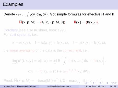
Examples
Denote 〈φ〉 :=∫
φ(y)dµx(y). Got simple formulas for effective H and h
H(x , p, M) = 〈H(x , ·, p, M, 0)〉, h(x) = 〈h(x , ·)〉.
Corollary [see also Kushner, book 1990]For split systems, i.e.,
σ = σ(x , y), f = f0(x , y) + f1(x , a), l = l0(x , y) + l1(x , a),
the linear averaging of the data is the correct limit, i.e.,
limε→0
uε(t , x , y) = u(t , x) := infα.
E[∫ t
0〈l〉(xs, αs) ds + 〈h〉(xt)
],
dxs = 〈f 〉(xs, αs) ds + 〈σσT 〉1/2(xs) dWs
Proof: H(x , p, M) = −trace(M〈σσT 〉)/2 + maxA {−〈f 〉 · p − 〈l〉} .
Martino Bardi (Università di Padova) Multi-scale Bellman-Isaacs Roma, June 15th, 2011 26 / 29

Example: we recover the Black-Scholes formula with stochasticvolatility.
In general, for system or cost NOT split,
H(x , p, M) = 〈maxA{...}〉 > max
A〈{...}〉
and the limit control problem is not obvious.We try to write H as a Bellman Hamiltonian in some other way in orderto find an explicit effective control problem approximating the singularlyperturbed one as ε → 0. We did it for
Merton problem with stochastic volatility (see next slides),
Ramsey model of optimal economic growth with (fast) randomparameters,
Vidale - Wolfe advertising model with random parameters,
advertising game in a duopoly with Lanchester dynamics andrandom parameters.
Martino Bardi (Università di Padova) Multi-scale Bellman-Isaacs Roma, June 15th, 2011 27 / 29
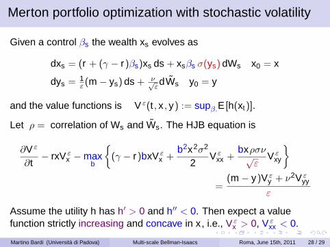
Merton portfolio optimization with stochastic volatility
Given a control βs the wealth xs evolves as
dxs = (r + (γ − r)βs)xs ds + xsβs σ(ys) dWs x0 = x
dys = 1ε (m − ys) ds + ν√
εdWs y0 = y
and the value functions is V ε(t , x , y) := supβ.E [h(xt)].
Let ρ = correlation of Ws and Ws. The HJB equation is
∂V ε
∂t− rxV ε
x −maxb
{(γ − r)bxV ε
x +b2x2σ2
2V ε
xx +bxρσν√
εV ε
xy
}=
(m − y)V εy + ν2V ε
yy
ε
Assume the utility h has h′ > 0 and h′′ < 0. Then expect a valuefunction strictly increasing and concave in x , i.e., V ε
x > 0, V εxx < 0.
Martino Bardi (Università di Padova) Multi-scale Bellman-Isaacs Roma, June 15th, 2011 28 / 29

The HJB equation becomes
∂V ε
∂t− rxV ε
x +[(γ − r)V ε
x + xρσν√ε
V εxy ]2
σ2(y)2V εxx
=(m − y)V ε
y + ν2V εyy
ε
By the Theorem, V ε(t , x , y) → V (t , x) as ε → 0 and V solves
∂V∂t
− rxVx +(γ − r)2V 2
x
2Vxx
∫1
σ2(y)dµ(y) = 0 in R+ × R+
This is the HJB equation of a Merton problem with the harmonicaverage of σ as constant volatility
σ :=
(∫1
σ2(y)dµ(y)
)−1/2
.
Therefore this is the limit control problem.
The limit of the optimal control βε,∗s as ε → 0 can also be studied.
Martino Bardi (Università di Padova) Multi-scale Bellman-Isaacs Roma, June 15th, 2011 29 / 29